Countering a fundamental law of attraction with quantum wavepacket engineering
Abstract
Bohmian mechanics was designed to give rise to predictions identical to those derived by standard quantum mechanics, while invoking a specific interpretation of it – one which allows the classical notion of a particle to be maintained alongside a guiding wave. For this, the Bohmian model makes use of a unique quantum potential which governs the trajectory of the particle. In this work we show that this interpretation of quantum theory naturally leads to the derivation of interesting new phenomena. Specifically, we demonstrate how the fundamental Casimir-Polder force, by which atoms are attracted to a surface, may be temporarily suppressed by utilizing a specially designed quantum potential. We show that when harnessing the quantum potential via a suitable atomic wavepacket engineering, the absorption by the surface can be dramatically reduced. This is proven both analytically and numerically. Finally, an experimental scheme is proposed for achieving the required shape for the atomic wavepacket. All these may enable new insights into Bohmian mechanics as well as new applications to metrology and sensing.
pacs
34.50.Dy, 03.75.KkI Introduction
Quantum mechanics (QM) challenges our common sense. For example, it allows superposition states which we never see directly, it adheres to a minimal uncertainty principle, and it is non-local. This has brought its own founding fathers, such as Schrödinger, Einstein and de Broglie, to speak against it. This has also given rise to many attempts to reinterpret it or even extend it. One of the attempts to reinterpret QM, and perhaps provide a base for future extensions of the theory, has been initially developed by de Broglie and Bohm, and has been termed Bohmian mechanics (BM) Bohm; BohmHiley; Holland; Cushing.

Over the last decade its proponents have shown it to have a relativistic form Durr99; Durr14, as well as a quantum field theory form BMQFT. Recently, several experimental studies have reported the observation of Bohmian trajectories Wiseman; Stein1; Stein2, but some have named these trajectories “surrealistic”Surr1; Surr2. Interestingly, several works have pointed out that using BM could help solving complex numerical problems in QM Solv1; Solv2; Solv3. However, the usefulness of this intriguing interpretation has remained under debate, and there does not seem to be a consensus yet as to the conceptual and practical merits of BM.
In this letter we show that the Bohmian quantum potential (defined in the next section) enables the engineering of new phenomena. Specifically we show how a fundamental force, the Casimir-Polder (CP) force, may be suppressed using this unique potential. This may enable new insights into the foundations of quantum theory, and may allow for new pathways in quantum technology applications, such as metrology and sensing. In particular, during the last two decades we have witnessed a major growth of experiments with cold atoms near surfaces. These experiments were driven by the desire to increase integration and scalability while miniaturizing these promising quantum devices, e.g. for various applications in metrology and atom interferometry Review1; Review2. The CP potential becomes important close to the surface, posing both fundamental and practical challenges. Recent works have utilized cold atoms to study the CP potential and examine atom-surface interactions Lin; Ketterle; Obr; Dalvit; Z1.
We utilize the quantum potential , which depends only on the shape of the wavefunction, to propose a special engineering of atomic wavepackets which enables them to partially resist the CP attraction to a nearby surface.
Within the next two sections we analyze, first analytically and then numerically, the proposed wavepacket engineering and its performance. We then briefly outline an experimental protocol for realizing this particular wavepacket.

II Suppressing the CP force via atomic wavepacket engineering
In what follows, we propose a theoretical method to effectively suppress the CP force (for a limited amount of time) through the generation of a tailored quantum potential. This method can be simply described when applying the Madelung transformation Mad following the recent analyses in Madelung; ShortT. BM, as well as the Madelung formalism, allow to efficiently describe the interplay between external potentials and the quantum potential and hence we find them very suitable in this case, where we try to counteract the former potentials.
We shall represent the wavefunction in the polar form
| (1) |
where and are the density and phase, respectively, and use the well-known guiding equation for the velocity
| (2) |
where the tilde superscript represents quantities per unit mass , so that . The real part of the Schrödinger equation then becomes the continuity equation
| (3) |
where , is the material (Lagrangian) time derivative of a fluid element along its trajectory, and the imaginary part becomes
| (4) |
where is the kinetic energy per unit mass and
| (5) |
is the quantum potential per unit mass.
For an irrotational potential flow in the form of Eq. 2, we then obtain
| (6) |
suggesting the possibility of cancelling an external potential using a suitable quantum potential .
Our proposed experimental setup consists of an atomic wavepacket . At time the wavepacket is brought close to the vicinity of a planar dielectric surface situated at using a harmonic trap (see Fig. 1). We assumed that the harmonic trap remained there also for , but assuming otherwise barely changed the simulated dynamics.
A CP potential acts on the atoms close to the dielectric surface, where is some constant depending on the properties of the surface and the atoms. Hereinafter we assume that the surface is the plane. We further assume that the wavepacket stays around the sub-micrometer distance from the surface but almost vanishes at the very close regime of about 100 nm from the surface, where the atom-surface interaction is dominated by the van der Waals potential, which has a dependence. We can therefore arrange the desirable situation , where the total acceleration of the atoms is zero, by preparing a density , which satisfies
| (7) |
In our proposed experimental setup we are only interested in the dynamics along the axis and hence our problem becomes one-dimensional (1D). In 1D, the solution of the ordinary differential equation corresponding to Eq. 11 is
| (8) |
See the Supplementary Material for additional details. We note that this wavefunction is continuous at , i.e. on the surface, and vanishes there. This function is not always positive but the physically meaningful field is. Our numerical simulations below indicate a slightly inferior performance of compared to and thus we use it hereinafter.
We now have to properly truncate the wavefunction for making it realistic (and square-integrable). This can be done, for instance, by multiplying it with a Gaussian envelope, thus reaching a wavepacket of the form
| (9) |
where the constants and and are the Gaussian’s mean and width, respectively. A wavefunction having this density will spread with time, but as was shown in ShortT, . Therefore, an initial preparation of a wavefunction according to Eq. 12 is a good estimation for short times, which is the regime we will numerically simulate below. For larger times, the wavepacket further spreads and becomes more and more distorted, thereby creating a different quantum potential which might be less beneficial. Using this technique a suitably prepared atomic wavepacket can be used, e.g., for measuring magnetic fields near the surface while passing above it, without being strongly drawn towards it.
For the short time spent by the wavepacket in the vicinity of the surface, this kind of truncation was shown in a similar context to be almost innocuous Siv. In our case, it hinders the cancellation of the CP potential as calculated in the Supplementary Material, but not fatally. The Gaussian truncation results in an unwanted residual potential (hereinafter there is no division by and hence no tildes are used) which is equal to
| (10) |
Although the residual potential is not negligible, its largest component near scales like , hence it suggests a major improvement in comparison to the CP potential which scales like close to the surface. Fig. 2 shows the weighted quantum potential, the weighted residual potential and the density of the engineered wavepacket.
Moreover, the inverse proportionality to guarantees that by increasing the width of the Gaussian envelope we can further shrink the overall size of the residual quantum potential. The term is also diverging, but if we average over the region of each singularity we will get a small contribution (sometimes in the form of a favorable repulsive potential). Therefore, and in contrast to the unengineered Gaussian, where the atoms are strongly attracted to the surface, here they will not be attracted so strongly. On the other hand, they may suffer from irregularities in the vicinity of the singularities and this is the reason that the numerical simulation performed below is important. Nevertheless, we may conclude on analytic grounds that while a solution of the form Eq. 8 could completely cancel the CP potential, the more realistic truncated shape in Eq. 12 also has the ability to suppress the CP force (for a limited amount of time).
III Numerical simulation
In order to study the performance of the proposed wavepacket engineering, we perform a numerical simulation examining the dynamics of the wavepacket in the vicinity of a dielectric surface. In particular, we wish to examine how the absorption of particles evolves in time when using engineered and unengineered wavepackets. The aim, of course, is to minimize the absorption when using an engineered wavepacket.
Below we briefly outline the details of the simulation and then compare the absorbed fraction achieved over time with our engineered atomic wavepacket (Eq. 12) to that of a Gaussian wavepacket.
To embed the proposed scheme within a more realistic setup, we are assuming that the atoms lie in a harmonic trap, situated close to the surface (throughout this work, the frequency of the harmonic trap is standardly determined by and ). The atoms are initially at rest. In addition, to simulate the absorption in the surface we assume, similarly to Scott, an imaginary potential growing linearly from zero at m till (implying that any atom that enters the region below m is absorbed within a certain time, unless having a sufficiently large velocity in the other direction), while the real part of the potential remains constant throughout m (we do require continuity in m).
This necessary modification of the total potential deteriorates the performance of our engineered wavepacket, which was not originally meant to resist it. However, as we shall show below, the simulative rate of absorption exhibited by the engineered wavepacket was still lower than that of the customary Gaussian wavepacket, which is consistent with the fact that the residual potential is much smaller than the CP potential near the surface.
We consider a 87Rb atom (mass kg) near a silicon surface (refractive index ). For the ground state static polarizability of 87Rb [ Hz/(V/c m)2] we have Jm4. We now solve the time-dependent Schrödinger equation for the atoms under the influence of the Casimir Polder + Harmonic + absorbing potentials. We run a simulation for a large set of means () and standard deviations (), and calculate the absorption fraction. Before the truncation, the sine and cosine solutions in Eq. 8 should give rise to the same quantum potential. However, the residual potential stemming from the truncation reveals that there is a difference between the two cases and we indeed notice some advantage of the cosine solution over the sine.
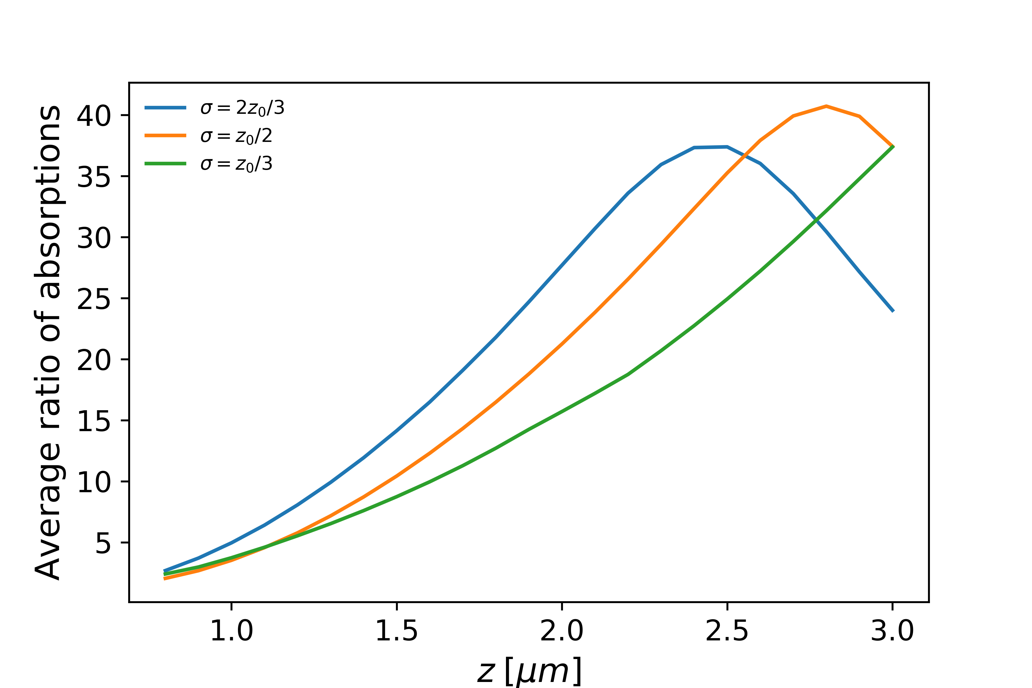
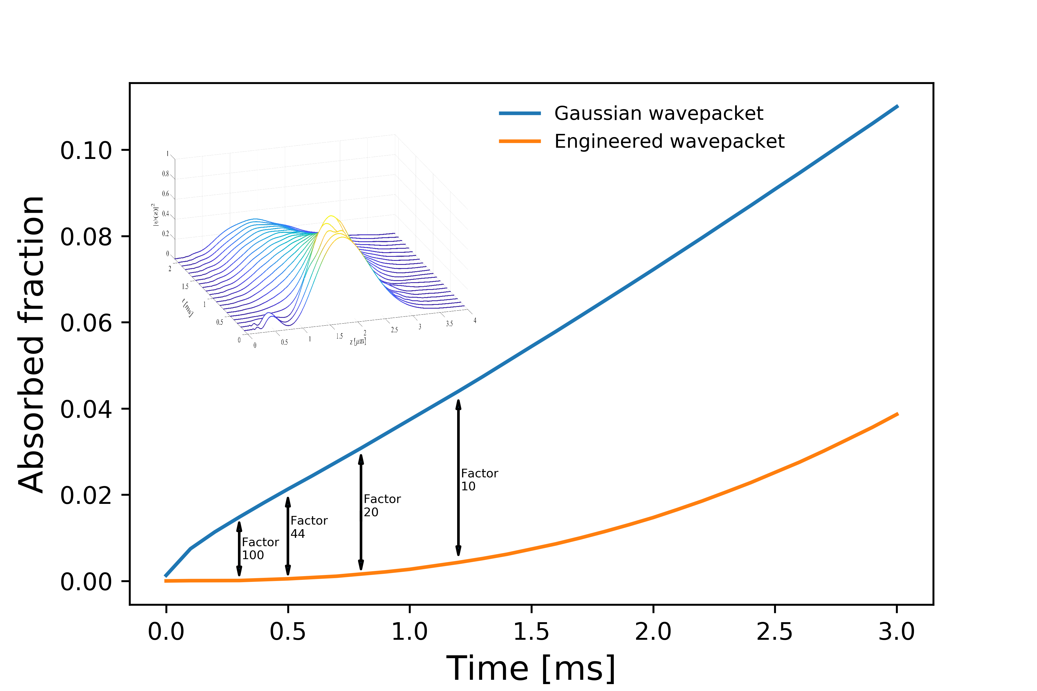
We compare for various cases our proposed solution in Eq. 12 to a Gaussian wavepacket with the same mean and standard deviation as those of the envelope – See Fig. 3. It is desirable, of course, to decrease as much as possible the residual potential, and since it contains three terms depending on , and , we have better results for higher- wavepackets. To further explore the advantage we choose some specific parameters (m and m) and compare the absorbed fractions – See Fig. 4.
As can be seen from Figs. 3 and 4, the engineered wavepacket leads to a significantly smaller absorbed fraction, which implies that the CP force has less impact on our engineered wavepacket in comparison to its impact on a Gaussian wavepacket. Thus, the results show that the engineered wavepacket’s shape indeed has the ability to reduce the unwanted effects of the CP force.
.
In accordance with our analytic expectations, the engineered wavepacket excels at high standard deviations and short times, reaching in some cases a 100-fold advantage over the Gaussian wavepackets in terms of absorption.
Note, however, that the engineered wavepacket is typically skewed away from the surface in comparison to the Gaussian envelope (and hence in comparison to the Gaussian wavepacket we used as a benchmark). Thus, one may ask whether the presented advantage follows only from this spatial displacement rather than the special shape of our wavepacket. To test this hypothesis we tried to fit a Gaussian wavepacket to the engineered solution by locating it farther away from the surface and/or shrinking its width until it highly resembled the Gaussian we compared it to. In all these cases we still found an advantage in favor of the engineered wavepacket (albeit smaller). We present such a comparison in the Supplementary Material, where we significantly pushed the Gaussian away from the surface. We still found that the engineered wavepacket has a substantially smaller absorbed fraction. Thus, we conclude that not only the shifted mean and modified width, but also the particular shape of the wavepacket contributed to the observed advantage.
Finally, we discuss the transient nature of the effect. As can be seen in Fig. 4, the absorption rate of the engineered wavepacket shows no advantage after about 3 ms. This is due to the fact that with time it loses its unique shape which originally gave rise to the required quantum potential. To show this explicitly, we plot in the inset of Fig. 4 the time evolution of the engineered solution from Eq. 12 with m and m. We can clearly see the amplitude decreasing with time and the shape being distorted.
.
IV A possible scheme for achieving the required wavepacket engineering
As was shown in the previous section, a certain shape of the wavepacket provides the desirable result, i.e. resisting the CP force for a short time. The construction of such a wavepacket can be obtained in several ways. We discuss here in general terms a technique which utilizes external potentials and fields (resembling Ron's).
First, a Gaussian atomic wavepacket can be prepared by cooling the atoms to occupy the Gaussian ground state of a harmonic potential. Engineering the wavepacket to the form of Eq. 12 may be done in two stages by utilizing an interferometric sequence with two internal atomic states having a different response to an external potential, e.g., due to a magnetic field. We use a magnetic field gradient pulse of duration to create a state-dependent spacially varying potential sandwiched between two properly designed Rabi pulses inducing transitions between the two states. These would be followed by a projection to one state, transforming the atomic wavepacket as . Here is the phase imprinted by the short pulse of potential difference between the two atomic states, while and are complex numbers determined by the Rabi pulses (we neglect a possible space-dependent global phase). In order to generate the linear -dependence in front of the right-hand-side of Eq. 12 we can apply a linear potential difference , choose , and obtain (if ). For generating the cosine (or sine) dependence with an argument proportional to we can apply a differential potential with a dependence, e.g. a magnetic field generated by a wire on the surface, and choose with a certain phase difference that determines the phase of the cosine function.
The resulting wavepacket, serving as a good approximation to Eq. 12 (for ), could now be used e.g. as an input for a magnetometry experiment near the dielectric surface without being strongly attracted to it.
V Discussion
In summary, we explored the possibility to use the Bohmian potential in order to cancel external potentials via wavepacket shaping. We have analytically proposed a novel technique that allows to suppress the CP force (for a limited period of time) and tested in numerically. Using this approach, we examined the case in which a Gaussian wavepacket is engineered into a special form such that near a dielectric surface the wavepacket resists the CP force. We have addressed the case of a wavepacket brought to a surface using a harmonic trap, but the presented analysis can be readily generalized to a grazing beam scenario (such as Z1). Although being related in the past to surreal phenomena, this work emphasizes the very real effects of the quantum potential, as well as its possible applications in practical scenarios. In addition to providing new insight concerning the Bohmian interpretation, this analysis may pave the way for various applications, e.g. surface magnetometry with cold atoms having engineered wavepackets which can survive longer at the vicinity of the surface. Although the CP potential was analyzed above, it should be noted that the useful interplay between external potentials and the quantum potential is general. Therefore, by carefully engineering the wavepacket, it is possible to suppress additional forces such as the gravitational or van der Waals forces.
References
- (1) D. Bohm, Phys. Rev. 85, 166-179 (1952).
- (2) D. Bohm, B. J. Hiley, The Undivided Universe: an Ontological Interpretation of Quantum Theory, Routledge, London (1993).
- (3) P. R. Holland, The quantum theory of motion: an account of the de Broglie-Bohm causal interpretation of quantum mechanics, Cambridge university press, Cambridge (1993).
- (4) J.T. Cushing, A. Fine, and S. Goldstein, Bohmian mechanics and quantum theory: an appraisal, Springer Science and Business Media, Dordrecht (1996).
- (5) D. Dürr, S. Goldstein, K. Münch-Berndl, and N. Zanghi, Phys. Rev. A 60, 2729 (1999).
- (6) D. Dürr, S. Goldstein, T. Norsen, W. Struyve, and N. Zanghi, Proc. R. Soc. A 470, 20130699 (2014).
- (7) D. Dürr, S. Goldstein, R. Tumulka, and N. Zanghi, Phys. Rev. Lett. 93, 090402 (2004).
- (8) H.M. Wiseman, New J. Phys. 9, 165 (2007).
- (9) S. Kocsis et al., Science 332, 1170 (2011).
- (10) D. Mahler et al., Sci. Adv. 2, e1501466 (2016).
- (11) B.G. Englert, M.O. Scully, G. Süssmann, and H. Walther, Z. Naturforsch. A 47, 1175-1186 (1992).
- (12) Y. Aharonov, B.G. Englert, and M.O. Scully, Phys. Lett. A 263, 137-146 (1999).
- (13) A.S. Sanz and S. Miret-Artés, J. Phys. A 44, 485301 (2011).
- (14) P. Botheron and B. Pons, Phys. Rev. A 82, 021404 (2010).
- (15) S. Garashchuk, J. Mazzuca and T. Vazhappilly, J. Chem. Phys. 135, 034104 (2011).
- (16) J. Fortágh and C. Zimmermann, Rev. Mod. Phys. 79, 235 (2007).
- (17) M. Keil, O. Amit, S. Zhou, S. Groswasser, Y. Japha, and R. Folman, J. Mod. Opt. 63, 1840-1885 (2016).
- (18) Y.J. Lin, I. Teper, C. Chin, and V. Vuletić, Phys. Rev. Lett. 92, 050404 (2004).
- (19) T.A. Pasquini et al., Phys. Rev. Lett. 97, 093201 (2006).
- (20) J.M. Obrecht, R.J. Wild, M. Antezza, L.P. Pitaevskii, S. Stringari, and E.A. Cornell, Phys. Rev. Lett. 98, 063201 (2007).
- (21) D.A.R. Dalvit, P.A.M. Neto, A. Lambrecht, and S. Reynaud, Phys. Rev. Lett. 100, 040405 (2008).
- (22) B.S. Zhao, H.C. Schewe, G. Meijer, and W. Schöllkopf, Phys. Rev. Lett. 105, 133203 (2010).
- (23) E. Madelung, Z. Phys. 40, 322 (1927).
- (24) E. Heifetz and E. Cohen, Found. Phys. 45, 1514 (2015).
- (25) M. de Gosson, B. Hiley, and E. Cohen, Ann. Phys. 374, 190-211 (2016).
- (26) G.A. Siviloglou and D.N. Christodoulides, Opt. Lett. 32, 979-981 (2007).
- (27) R.G. Scott, A.M. Martin, T.M. Fromhold, and F.W. Sheard, Phys. Rev. Lett. 95, 073201 (2005).
- (28) M. Nest, Y. Japha, R. Folman, R. Kosloff, Phys. Rev. A 81, 043632 (2010).
VI Methods
VI.1 The engineered wavepacket and the total potential
The engineered wavepacket we employed is given by the solution of
| (11) |
multiplied by a Gaussian truncation , yielding
| (12) |
In our numerical simulation we assumed that the wavepacket is brought to the vicinity of the dielectric surface using a harmonic potential which remains there. Then, following Scott, the Casimir-Polder potential is acting on the wavepacket for any m. For m it is replaced by a constant value, (assuring continuity at m), and a linear imaginary potential is added as in Scott.
VI.2 Calculation of the residual potential
We shall compute here the residual quantum potential corresponding to our proposed construction. This will allow us to investigate more deeply the analytic properties of the shaping, which are important for any experimental demonstration of this technique.
In 1D, the solution of our ordinary differential equation takes the form (12). For simplicity we define the following function
| (13) |
We shall now compute the value of
| (14) |
where . That is
| (15) |
and after some algebraic calculations
| (16) |
From the fact that we have
| (17) |
VI.3 Comparison to a fitted Gaussian
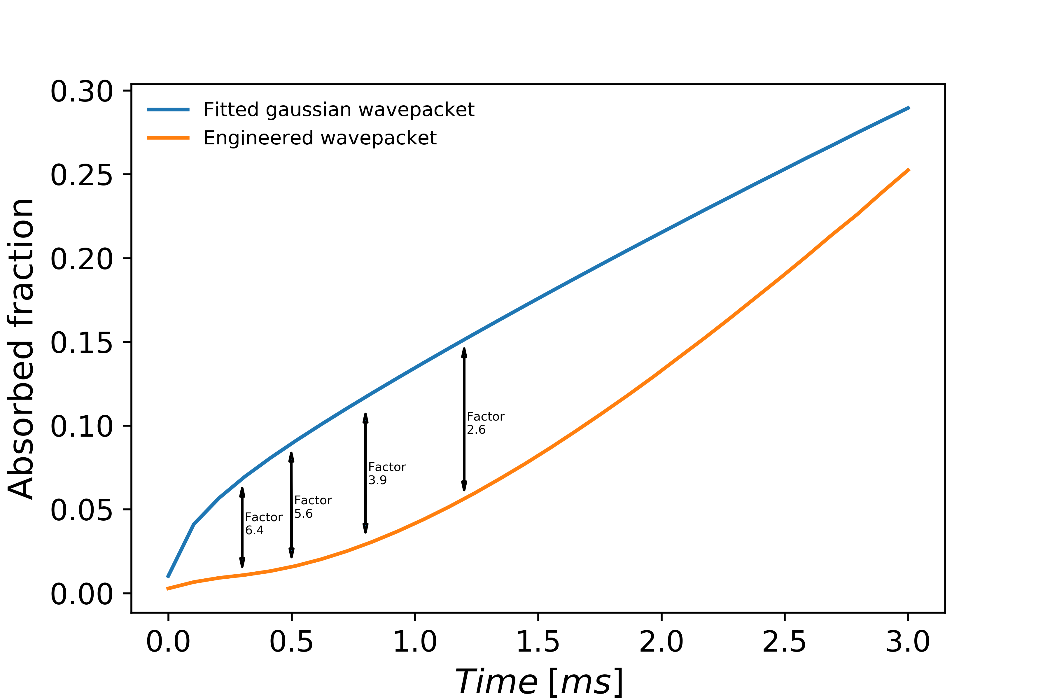
To verify that the advantage reported in the main text, in terms of absorption, stems from the shape and not only the bias of the engineered wavepacket away from the surface, we compare in Fig. 5 the absorption of the engineered solution to the absorption of a fitted Gaussian located at the same distance from the dielectric surface. The advantage is smaller, but still apparent.