Boost-S: Gradient Boosted Trees for Spatial Data and Its Application to FDG-PET Imaging Data
Abstract
Boosting Trees are one of the most successful statistical learning approaches that involve sequentially growing an ensemble of simple regression trees (i.e., “weak learners”). This paper proposes a new gradient Boosted Trees algorithm for Spatial Data (Boost-S) for spatially correlated data with covariate information. Boost-S integrates the spatial correlation structure into the classical framework of gradient boosted trees. Each tree is grown by solving a regularized optimization problem, where the objective function involves two penalty terms on tree complexity and takes into account the underlying spatial correlation. A computationally-efficient algorithm is proposed to obtain the ensemble trees. The proposed Boost-S is applied to the spatially-correlated FDG-PET (fluorodeoxyglucose-positron emission tomography) imaging data collected during cancer chemoradiotherapy. Our numerical investigations successfully demonstrate the advantages of the proposed Boost-S over existing approaches for this particular application.
Key words: Gradient Boosted Trees, Spatial Statistics, FDG-PET, Chemoradiotherapy
Introduction
Spatial data refer to an important type of data which arise in a spatial area and are often correlated in space. Capturing such correlation is the centerpiece of statistical analysis of spatial data (Cressie and Wikle 2011b; Schabenberger and Gotway 2005). Applications of statistical spatial data modeling can be found in a spectrum of scientific and engineering applications ranging from energy (Ezzat et al. 2019), reliability (Liu et al. 2018c; Fang et al. 2019), quality and manufacturing (Zang and Qiu 2019; Wang et al. 2016; Yue et al. 2020), environmental and natural process (Guinness and Stein 2013; Liu et al. 2018a; Liu et al. 2020), medical informatics (Yao et al. 2017; Yan et al. 2019), etc.
The Problem Statement
In this paper, we are concerned with the modeling problem:
| (1) |
where represents the observation at a spatial location , is a vector that collects the available features at , is the mean-value function given , and is an isotropic and weakly stationary spatial noise process with zero-mean and a covariance , where with being some distance measure between and ; for example, the Euclidean distance.
The goal of this paper is to tackle the modeling problem (1) by devising a new additive-tree-based method that approximates as follows:
| (2) |
where represents an ensemble of binary decision trees, and represents the tree space.
Apparently, the problem hinges on how the ensemble of trees can be grown, while taking into account the important spatial correlation of . In particular, we exploit the idea of gradient boosting which involves sequentially growing an ensemble of simple regression trees. Mathematically, each tree is added to the ensemble by solving an optimization problem with a carefully chosen objective function. This goal boils down to three fundamental tasks to be addressed in this paper: (i) formulate a (regularized) optimization problem that balances the complexity of individual trees and takes into account the spatial correlation associated with ; (ii) devise an algorithm that solves the regularized optimization problem in a computationally efficient manner (so that trees can be added sequentially to the ensemble); and (iii) validate the performance of the proposed method on real datasets.
A Motivating Application
A motivating application is first presented. Fluorodeoxyglucose-Positron Emission Tomography (FDG-PET) has been widely used in cancer diagnosis and treatment to detect metabolically active malignant lesions, and plays a critical role in quantitatively assessing and monitoring tumor response to treatment. For illustrative purposes, Figure 1 shows the Standardized Uptake Values (SUV) obtained from the FDG-PET imaging of a patient. In this figure, the top row shows the baseline image taken before the radiotherapy (i.e., Pre-RT), while the bottom row shows the FDG PET/CT imaging 3 weeks after radiotherapy (i.e., Mid-RT image). In this case, it is possible to observe the shrinkage of the tumor, indicating the effectiveness of treatment. Hence, the difference between the Mid-RT and Pre-RT images can be naturally used to quantify the tumor’s spatial response to treatment. Figure 1 also suggests that a tumor typically presents spatially-correlated and spatially-heterogeneous responses. Some areas of a tumor may respond well to treatment while some areas appear to be less responsive. The importance of capturing such spatially-varying and spatially-correlated responses has been discussed in Bowen et al. 2019.


A tumor is a three-dimensional object. Figure 2 shows the SUV in three-dimensional spaces for another two patients. The top row shows the Pre-RT data, while the bottom row shows the Mid-RT data collected 3 weeks after the radiotherapy. It is seen that,
- •
The overall SUV level decreases 3 weeks after the radiotherapy;
- •
The change in SUV (i.e., tumor’s response to radiotherapy) varies over space. In particular, the SUV level gradually decreases from the centroid to the surface of a tumor.
Hence, if we let in (1) represent the change in SUV level at location within the spatial domain occupied by the tumor, then, a statistical spatial model is needed that enables clinicians to understand how depends on a vector of features (including geometric features, therapy dosage, and so on) for treatment optimization and control. However, in practice, the complex relationship between the response and features can hardly be directly specified. The inevitably nonlinear and interaction effects motivate us to investigate the non-parametric tree-based methods in this paper. More detailed discussions and rationales are provided in the next section.
Literature Review and Contributions
The pioneering work of statistical modeling of spatial data can be found in Banerjee et al. 2004, Schabenberger and Gotway 2005 and Cressie and Wikle 2011a. The mainstay approach, also known as the geostatistical paradigm, models spatial processes by random fields with fully specified covariance functions. A linear relationship between covariates and process mean is often assumed, and the model parameters can be obtained through Generalized Least Squares or Maximum Likelihood Estimation. The covariance structures are typically derived from moments of multivariate probability distributions and motivated by considerations of mathematical convenience (e.g., stationary, isotropic, space-time separable, etc.). Hence, there have been prolonged research interests to provide flexible and effective ways to construct non-stationary covariance functions (Cressie and Huang 1999; Gneiting 2002; Fuentes et al. 2005; Gneiting et al. 2006; Ghosh et al. 2010; Reich et al. 2011; Lenzi et al. 2019). The geostatistical modeling paradigm, which heavily relies on random fields, becomes less practical for large problems and approximations are commonly used, such as the Gaussian Markov Random Fields representation (Lindgren and Rue 2011), Nearest-Neighbor Gaussian Process (Datta et al. 2016; Banerjee 2017), kernel convolution (Higdon 1998), low-rank representation (Cressie and Johannesson 2002; Nychka and Wikle 2002; Banerjee et al. 2008), the approximation of likelihood functions (Stein et al. 2004; Fuentes 2007; Guinness and Fuentes 2015), Bayesian inference for latent Gaussian models based on the integrated nested Laplace approximations (Rue et al. 2009; R-INLA 2019), Lagrangian spatio-temporal covariance function (Gneiting et al. 2006), matrix-free state-space model (Mondal and Wang 2019), Vecchia approximations of Gaussian processes (Katzfuss et al. 2020), as well as the multi-resolution approximation (M-RA) of Gaussian processes observed at irregular spatial locations (Katzfuss 2017).
Other spatial models have also been proposed in the literature. Notably, the Markov Random Fields (MRF) model focuses on the (conditional) distribution of the quantity at a particular spatial location given the neighboring observations, such as the auto Poisson model (Besag 1974), Conditional Autoregressive Model (Carlin and Banerjee 2003; Liu et al. 2018b), etc. The Spatial Moving Average (SMA) approach models a spatial process through a process convolution with a convolution kernel (Higdon 1998; Brown et al. 2000; Liu et al. 2016). There is also a large body of literature focusing on spatio-temporal data. For example, the Hierarchical Dynamical Spatio-Temporal Models (DSTM) (Wikle and Cressie 1999; Berliner 2003; Cressie and Wikle 2011a; Stroud et al. 2010; Katzfuss et al. 2020), and the SPDE-based modeling approach that aims to integrate governing physics into statistical spatio-temporal models (Brown et al. 2000; Hooten and Wikle 2008; Stroud et al. 2010; Sigrist et al. 2015; Liu et al. 2020). A summary of the latest advances in the spatial modeling with SPDE can be found in Cressie and Wikle 2011a and Krainski et al. 2019.
For spatial models in the form of (1), one challenge arising from practice is to specify the relationship between the covariates and response , which can rarely be adequately captured by linear models. For the FDG-PET imaging data presented in Section 1.2, for example, both non-linear and interaction effects are expected between tumor’s response and covariates (such as treatment, geometric features of the tumor, etc.). Hence, non-parametric approaches, especially the additive-tree-based approaches, provide some major modeling advantages. Constructing a tree does not require parametric assumptions on the complex relationship between features and event processes. An individual tree performs a partition of the feature space. For each sub feature space, a predicted value is found for the individuals over that sub feature space. A sum-of-trees model consists of multivariate components that effectively handle the complex interaction effects among features (Chipman et al. 2010). Feature selection is also possible under the framework of additive-tree-based models (Hastie et al. 2009; Liu and Pan 2020).
Among the additive-tree-based methods, gradient boosted trees have become one of the most successful statistical learning approaches over the last two decades, generating 17 winning solutions among 29 Kaggle challenges in 2015 (Chen and Guestrin 2016). Schapire 1999 introduced the first applicable Boosting method. The main idea of gradient boosting hinges on fitting a sequence of correlated “weaker learners” (such as simple trees). Each tree explains only a small amount of variation not captured by previous trees (Hastie et al. 2009; Chipman et al. 2010). However, many existing boosting trees, such as XGBoost, do not consider the possible spatial correlation when they are applied to spatial data. To our best knowledge, Sigrist 2020 recently proposed the only boosted-trees-based approach for Gaussian Process and mixed effects model (which captures correlated errors). Such a method minimizes the negative log-likelihood at each tree node splitting, and is available in the R package, GPBoost. The package also provides a range of regularization and tuning parameter options. In our paper, on the other hand, regularizations have been directly added to the objective function in order to control the complexity of individual trees (i.e., number of leaves and leaf weights), leading to a regularized optimziation problem at each tree node splitting. The regularization terms are motivated by the fundamental idea behind boosting trees which involves a sequence of correlated simple trees. This idea has been adopted by XGBoost (Chen and Guestrin 2016), while an alternative approach adopted by the Bayesian Additive Regression Trees (BART) involves assigning prior distributions on parameters charactering the tree structure (Chipman et al. 2010). Hence, the main contribution of the paper is to propose a computationally-efficient gradient boosting method for growing the ensemble trees in (2) for spatially-correlated data. Each tree is grown by solving a regularized optimization problem, where the objective function involves regularizations on tree complexity and takes into account the underlying spatial correlation. The proposed algorithm is referred to as Boost-S, which stands for Gradient Boosted Trees for Spatial Data with covariate information (Boost-S). Boost-S integrates the spatial correlation structure into the classical framework of gradient boosted trees. In Statistics, Ordinary Least Squares is extended to Generalized Least Squares for correlated data. An analogous notion can be formulated here when extending the classical framework of gradient boosted trees to spatially-correlated data, giving rise to the proposed Boost-S.
Boost-S: Technical Details
This section provides the technical details behind Boost-S. Suppose that data are collected from a number of spatial locations, . At each location, we observe a response and a -dimensional feature vector . From (1) and (2), Boost-S aims to construct an ensemble of binary trees, , using gradient boosting such that
| (3) |
Let be a multivariate random vector representing the responses from the spatial locations, and let be a vector of predicted values at the spatial locations generated from the th tree (), we re-write (3) as
| (4) |
where is a vector of zeros corresponding to the initial condition when no tree has been grown.
A Regularized Problem
This subsection presents the detailed tree structures and formulates a regularized optimization problem that leads to a sequence of ensemble trees. In (3), each tree is a Classification and Regression Tree (CART) that resides in a binary tree space
| (5) |
where and . Here, represents the number of tree leaves (i.e., terminal nodes), is the value on a tree leaf (i.e., leaf weight), and determines the tree structure (i.e., a mapping that links a feature vector to a tree leaf).
Suppose that a number of trees have been grown (). Then, the (ensemble) predicted values at the spatial locations are given by from the trees. An immediate next step is to construct the th tree and add the new tree to the ensemble such that . For binary trees, this involves finding the optimal split features as well as the split points for the th tree. This task can be formulated as a regularized optimization problem:
| (6) |
where is a loss function that depends on the output of the th tree, and the regularization is given by:
| (7) |
The first term, , regularizes the depth of the tree (by penalizing the total number of leaves), while the second term is used to regularize the contribution of tree to the ensemble predictions (by penalizing the weights on tree leaves). Recall that, the fundamental idea behind boosting trees is to construct a sequence of correlated “weaker learners” (i.e., simple trees), where each “weaker learner” is added to explain the unexplained variation by existing trees in the ensemble (Chipman et al. 2010). Hence, the regularization (7) effectively controls the complexity of individual trees. In fact, it is worth noting that the regularization also helps to prevent the well-known overfitting issue of boosting trees. When a sufficient number of trees have been included in the ensemble, the penalty of adding one more tree may dominate the benefit (of adding more trees), which stops the algorithm from growing more trees.
Because the multivariate response is spatially correlated with the covariance matrix , a sensible choice for the loss function is the squared Mahalanobis length of the residual vector:
| (8) |
and (6) can thus be written as
| (9) |
Note that, (9) above extends the classical XGBoost which does not consider the correlation among the elements of (Chen and Guestrin 2016). The extension made by this paper is in analogy to the extension from Ordinary Least Squares to Generalized Least Squares. However, such an extension requires new algorithms for the problem (9) to be efficiently solved.
The regularized optimization above is a formidable combinatorial optimization problem which can hardly be directly solved. Hence, we approximate the objective function by a second-order multivariate Taylor expansion:
| (10) |
where is the column gradient vector of the loss function with its th element given by , and is the Hessian matrix with its th entry being given by . Because the first term on the right-hand-side of (10) is a constant, it is sufficient to minimize the sum of the remaining three terms:
| (11) |
Note that, for any given tree structure, it is possible to define a set that consists of all samples that fall into leaf . Then, we let be a column vector that only retains the elements in corresponding to samples in , and similarly, let be a matrix by only keeping the rows and columns of corresponding to samples in and , respectively.
Figure 3 provides an illustration of how and are constructed. Consider a simple example where (i.e., only 7 samples are available), then, the dimensions of the gradient vector and the Hessian matrix are and , respectively. Suppose that and . Then, the vector consists of the 1st, 2nd and the 6th element in , and the matrix is a matrix that retains the entries located at the intersections of rows 1, 2 and 6, and columns 3 and 4.

Then, for any given tree structure , we re-write (11) as follows:
| (12) | |||
where denotes the combination (i.e., the number of 2-combinations from a given set of elements), with and respectively being the weight on tree leaf and a column vector of ones of dimension , and represents the cardinality of a set.
Taking the partial derivatives of (13) with respect to leads to a system of equations, which provides the key computational advantage: given any tree structure, the optimal weights can be quickly found by solving the linear system:
| (14) |
where is a matrix with its th row given by
| (15) |
and is a vector with its th element given by .
Obtaining the linear system (14) plays an extremely important role in searching for the optimal tree: given any candidate tree structure, it is possible to quickly and accurately find the optimal weights on the leaf nodes by solving (14) using least squares, i.e., no numerical search is required. By substituting the optimal into (11) immediately yields the value of the objective function .
The Sequential Update of the Unknown Covairance Matrix
Constructing the linear system (14) and evaluating the objective function require a known covariance matrix of the errors, . However, is not known and needs to be estimated before the first tree (), or any subsequent tree (), can be constructed. In this section, we describe how can be consistently estimated before the th tree is constructed, given the outputs from the first trees.
Suppose that trees have been constructed (), and let be the residual vector. It follows from (4) that is Gaussian with the covariance . Note that, the mean of may not even be close to zero when is small, i.e., when there are not sufficient trees in the ensemble to well capture the mean of . In this case, we model by a Locally Weighted Mixture of Linear Regressions (LWMLR) (Stroud et al. 2001):
| (16) |
where is a set of spatial basis functions, is a vector of unknown coefficients, is a Gaussian kernel given as follows:
| (17) |
Note that, we may re-write (16) as a linear model, , where , , and . Then, it is possible to obtain a consistent estimate of , , using the Feasible Generalized Least Square (FGLS), before the th tree can be constructed.
The Boost-S Algorithm
Following the discussions above, Figure 4 provides a high-level illustration of the flow of the Boost-S algorithm. At the initialization stage, we obtain the initial estimate of the covariance matrix . Then, by solving the regularized optimization problem (6), a new tree is constructed and added to the ensemble. Next, the estimate of the covariance matrix is updated before tree can be constructed. The steps are repeated until trees have been grown in the ensemble. The Boost-S algorithm is formalized by Algorithm 1.
(i) Given the current tree topology, generate a set of all possible new tree structures by splitting a tree node based on candidate split variables and candidate split values.
(ii) For each new tree structure, obtain the weights on the leaf nodes by solving the linear system , and evaluate the objective function in (11) for the new topology.
(iii) If there exists at least one new tree structure that further reduces the objective function (over the existing tree structure), retain the new topology that generates the greatest reduction and go to (i); otherwise, terminate the tree growing process for tree , and go to the next step.
(iv) Update the estimate using FGLS. end for
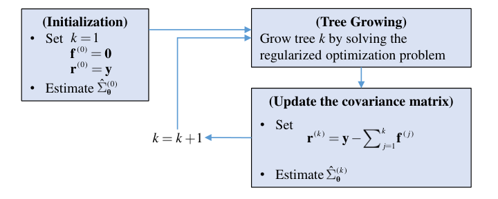
Illustration of Boost-S on the FDG-PET Imaging Data
This section re-visits the motivating application presented in Section 1.2. We apply Boost-S to real datasets and compare the performance of Boost-S to that of existing approaches.
Data
The data used in this section are obtained from 25 patients diagnosed with locally advanced and surgically unresctable non-small cell lung cancer (NSCLC) who enrolled onto the FLARE-RT clinical trial (NCT02773238). For each patient, this clinical trial data set contains geographic features, dosage, Pre-RT and Mid-RT SUV levels. As discussed in Section 1.2, the goal is to model the difference between the Pre-RT SUV (before treatment) and Mid-RT SUV (during third week of treatment course), which helps clinicians further optimize or control the treatment plans.
Let represent the ratio between Mid-RT SUV and Pre-RT SUV at location (a voxel in the image) within the spatial domain occupied by the tumor, i.e.,
| (18) |
If the treatment is effective, the Mid-RT SUV is expected to be lower than the Pre-RT SUV level. Hence, a lower ratio indicates more effective treatment.
Application of Boost-S
We first demonstrate the application of Boost-S on the data collected from one of the 25 patients. The PET scan for this patient has 3110 voxels (i.e., the number of spatial locations). We randomly split the data into two parts: 15% for training while 85% for testing. Such a low training-testing ratio is chosen to demonstrate the out-of-sample prediction capability of Boost-S constructed from a relatively small training dataset.
To obtain the initial estimate of the covariance matrix , the FGLS is used to solve the linear model (16) in Algorithm 1. Before the FGLS is performed, one needs to first choose a parametric spatial covariance function of the process in (16). Figure 5 shows both the empirical semivariance and the fitted semivariance using FGLS assuming the Gaussian covariance function. The sill, range and nugget effect can be clearly seen from Figure 5, and the Gaussian covariance function appears to be an appropriate choice.
Algorithm 1 requires the tuning parameters and to be pre-specified. The choice of these two parameters affects both the depth and contribution of individual trees to the ensemble prediction, which in turn influences the total number of trees in the ensemble. A common strategy suggests that we explore the suitable values for and while leaving as the primary parameter (Hastie et al. 2009). Although it is theoretically possible to perform a grid search for the best combinations of and on a two-dimensional space, such an approach may not be practical nor necessary in practice when it is computationally intensive to run Boost-S on big datasets. Hence, we resort to a powerful tool in computer experiments—the space-filling designs (Joseph 2016). The idea of space-filling designs is to have points everywhere in the experimental region with as few gaps as possible, which serves our purpose very well. Figure 6 shows the Maximum Projection Latin Hypertube Design (MaxProLHD, Joseph et al. 2015) of 16 runs with different combinations of and , where the experimental ranges for these two parameters are respectively and . For each design, Figure 7 shows the box plot of the number of tree leaves per tree in an ensemble for each combination of and . Since the key idea behind boosting trees is that each individual tree needs to be kept simple (Hastie et al. 2009), we identify that Designs #7, #8 and #9 provide the most suitable combinations of and . From Figure 6, these three design points are adjacent to each other, indicating that the appropriate choices for and are approximately within and . A refined search in a much smaller experimental region yields an appropriate combination of and (Design “” in Figure 6). Design “” is between Designs #7 and #8, and the 25th, 50th and 75th empirical quartiles of the number of tree leaves are 6, 8 and 10 as shown in Figure 7.
After and have been appropriately chosen, 49 trees are constructed to form the ensemble predictor using Algorithm 1. Figure 8 (top panel) shows that the Mahalanobis distance (i.e., the objective function) decreases as more trees have been included into the ensemble, indicating that the algorithm is working as expected. Figure 8 (bottom panel) shows the number of tree leaves for individual trees in this ensemble. It is interesting to note that the algorithm no longer splits the (root) tree node after 37 trees have been grown. In addition, the outputs of these one-node trees are all zeros, indicating that all trees after tree 37 are completely redundant. This is precisely due to the regularization and in (6). The gain in is outweighted by the loss caused by if one more tree is added.
Applying the constructed ensemble trees to the testing dataset, Figure 9 shows the out-of-sample Root-Mean-Square-Error (RMSE) and Mean-Gross-Error (MGE). We see that both performance metrics decrease as more trees are included and stabilize approximately after 30 to 40 trees have been grown. As discussed above, this is precisely due to the fact that all trees after #37 are redundant with zero output. Figure 10 shows the (out-of-sample) predictions against actual observations of the SUV level at differnt voxels. The figure shows that the proposed Boost-S accurately predicts the SUV levels given the covariate information.

Furthermore, we reconstruct the Mid-RT SUV (3 weeks after treatment) by the proposed Boost-S, and compare the actual and predicted Mid-RT SUV using slice plots (Figure 11). Because a tumor is a 3D object with three coordinates, , , and , the MidPET images are shown on the plane for given values of . We see that the ensemble trees are capable of predicting the Mid-RT SUV for the entire tumor body.
Comparison Study
We compare the predictive capability of Boost-S to five other methods using the data collected from 25 patients. The five other methods included in the comparison study are: Random Forests (RF) (Breiman 2001), Extreme Gradient Boosting Trees (XGBoost) (Chen and Guestrin 2016), non-parametric cubic splines, universal kriging with a linear spatial trend, and multiple linear regression without considering the spatial correlation. For each patient, 15% of the observations are randomly chosen as the training dataset, and all 6 models are constructed to generate the out-of-sample predictions using the testing dataset. Such a low training-testing ratio is used to test the predictive capabilities of these methods.
Tables 1, 2 and 3 respectively show the Mean Gross Error (MGE), Relative Error (RE) and Rooted Mean Squared Error (RMSE) of the out-of-sample predictions for 25 patients using 6 different methods. It is interesting to see that
- •
The proposed Boost-S yields the lowest MGE for 19 out of the 25 patients, while RF performs the best for the remaining 6 patients;
- •
The proposed Boost-S yields the lowest RE for 18 out of the 25 patients, while RF performs the best for the remaining 7 patients;
- •
The proposed Boost-S yields the lowest RMSE for 17 out of the 25 patients, while RF performs the best for the remaining 8 patients;
Hence, we conclude that, the proposed Boost-S provides the best performance for majority of the patients in terms of all three performance measures, although no method uniformly outperforms others (which is realistic and expected given the well-known modeling power of RF and XGBoost). The reason why Boost-S outperforms other additive-tree-based methods, i.e., RF and XGBoost, is because of its capability of accounting for the spatial correlation among observations. The reason why Boost-S outperforms universal Kriging and multiple linear regression is due to the advantages of non-parametric tree-based method in capturing complex non-linear and interaction effects between features and responses. The observation demonstrates the effectiveness of Boost-S as a useful extension to existing ensemble tree-based methods by accounting for the spatial correlation among observations.
| Boost-S | RF | XGBoost | Cubic Splines | Universal Kriging | Linear Regression |
| 8.24 | 6.78 | 7.31 | 8.45 | 10.32 | 9.01 |
| 10.68 | 9.61 | 10.55 | 11.57 | 13.41 | 13.79 |
| 5.84 | 6.22 | 6.32 | 7.14 | 10.37 | 9.08 |
| 4.30 | 4.37 | 4.68 | 6.19 | 6.76 | 6.20 |
| 3.15 | 4.45 | 3.97 | 4.70 | 10.04 | 8.58 |
| 1.95 | 2.40 | 2.51 | 3.07 | 5.42 | 4.25 |
| 5.20 | 5.40 | 5.67 | 5.47 | 13.30 | 10.34 |
| 5.04 | 5.30 | 5.93 | 9.00 | 10.39 | 9.88 |
| 8.59 | 9.28 | 9.50 | 9.22 | 12.55 | 11.79 |
| 2.37 | 2.79 | 3.17 | 4.46 | 6.70 | 5.97 |
| 9.08 | 8.63 | 8.91 | 11.16 | 10.79 | 11.22 |
| 1.44 | 1.74 | 2.08 | 2.64 | 4.00 | 2.99 |
| 1.65 | 1.91 | 2.08 | 3.61 | 4.36 | 3.69 |
| 0.74 | 1.32 | 1.35 | 1.58 | 2.48 | 1.83 |
| 10.19 | 9.77 | 10.59 | 10.98 | 15.03 | 13.71 |
| 4.17 | 4.37 | 4.25 | 7.79 | 9.64 | 7.89 |
| 2.71 | 3.20 | 3.78 | 4.22 | 7.15 | 6.47 |
| 6.53 | 7.06 | 8.27 | 8.41 | 13.43 | 12.18 |
| 13.10 | 10.62 | 11.36 | 12.57 | 13.77 | 14.23 |
| 3.51 | 3.96 | 4.06 | 4.44 | 9.30 | 6.85 |
| 1.22 | 1.24 | 1.57 | 1.58 | 2.55 | 2.03 |
| 4.17 | 4.82 | 5.01 | 7.69 | 11.25 | 8.71 |
| 5.47 | 6.62 | 6.43 | 10.65 | 18.82 | 12.05 |
| 3.87 | 3.63 | 4.13 | 5.08 | 5.52 | 5.47 |
| 1.86 | 2.42 | 2.58 | 3.57 | 5.60 | 4.19 |
| N.A. | 0.04 | 0.001 |
| Boost-S | RF | XGBoost | Cubic Splines | Universal Kriging | Linear Regression |
| 9.67 | 8.01 | 8.58 | 9.91 | 12.29 | 10.68 |
| 56.62 | 51.01 | 55.37 | 60.03 | 60.47 | 67.27 |
| 11.04 | 12.52 | 11.93 | 13.72 | 18.40 | 17.01 |
| 5.03 | 5.34 | 5.53 | 7.60 | 8.36 | 7.61 |
| 7.30 | 9.41 | 8.26 | 10.77 | 20.25 | 19.07 |
| 4.42 | 5.73 | 5.65 | 7.29 | 12.52 | 9.72 |
| 8.92 | 9.41 | 9.52 | 9.72 | 20.53 | 18.06 |
| 23.25 | 22.32 | 25.52 | 43.34 | 43.51 | 43.78 |
| 13.62 | 15.45 | 15.18 | 14.45 | 20.04 | 18.91 |
| 2.28 | 2.74 | 3.07 | 4.26 | 6.48 | 5.77 |
| 11.44 | 10.78 | 10.94 | 14.42 | 13.41 | 14.39 |
| 1.09 | 1.32 | 1.55 | 1.99 | 3.06 | 2.25 |
| 3.66 | 4.25 | 4.55 | 8.00 | 9.70 | 8.20 |
| 1.49 | 2.75 | 2.72 | 3.17 | 4.70 | 3.59 |
| 21.40 | 19.97 | 21.21 | 23.26 | 32.02 | 29.69 |
| 8.36 | 8.67 | 8.13 | 15.27 | 20.18 | 15.49 |
| 3.90 | 4.68 | 5.34 | 6.05 | 9.93 | 9.51 |
| 7.46 | 8.79 | 9.97 | 9.99 | 17.54 | 15.31 |
| 21.70 | 17.32 | 18.19 | 20.08 | 21.71 | 23.53 |
| 4.02 | 4.58 | 4.60 | 5.05 | 10.15 | 7.95 |
| 1.91 | 1.94 | 2.43 | 2.53 | 4.08 | 3.24 |
| 6.34 | 7.18 | 7.61 | 11.55 | 17.54 | 13.37 |
| 8.10 | 9.55 | 8.73 | 16.69 | 25.45 | 18.96 |
| 5.24 | 5.01 | 5.63 | 7.10 | 7.85 | 7.61 |
| 5.07 | 6.59 | 6.86 | 9.72 | 14.92 | 11.26 |
| N.A. | 0.09 | 0.004 |
| Boost-S | RF | XGBoost | Cubic Splines | Universal Kriging | Linear Regression |
| 11.05 | 9.01 | 9.66 | 10.89 | 13.00 | 11.66 |
| 16.46 | 14.77 | 16.22 | 16.14 | 19.66 | 19.42 |
| 7.73 | 7.83 | 8.10 | 9.17 | 12.89 | 11.61 |
| 5.74 | 5.51 | 5.89 | 7.73 | 8.28 | 7.74 |
| 4.13 | 5.97 | 5.41 | 6.00 | 12.83 | 10.64 |
| 2.68 | 3.11 | 3.24 | 3.89 | 6.68 | 5.36 |
| 7.03 | 6.68 | 7.13 | 6.98 | 17.10 | 12.64 |
| 7.62 | 7.88 | 8.58 | 11.50 | 14.09 | 13.07 |
| 11.15 | 11.69 | 12.02 | 11.80 | 15.57 | 15.04 |
| 3.21 | 3.80 | 4.32 | 5.97 | 8.28 | 7.66 |
| 12.52 | 12.06 | 12.41 | 14.47 | 14.68 | 14.87 |
| 1.89 | 2.20 | 2.64 | 3.64 | 4.75 | 4.02 |
| 2.20 | 2.46 | 2.66 | 4.56 | 5.10 | 4.68 |
| 1.04 | 1.69 | 1.72 | 1.95 | 3.21 | 2.37 |
| 14.17 | 13.19 | 14.17 | 14.29 | 18.66 | 17.32 |
| 5.77 | 5.94 | 5.71 | 10.18 | 12.27 | 10.31 |
| 3.48 | 4.15 | 4.73 | 5.30 | 8.99 | 8.28 |
| 8.72 | 8.98 | 10.50 | 10.83 | 16.69 | 15.26 |
| 19.26 | 15.23 | 16.30 | 17.69 | 20.01 | 19.80 |
| 5.02 | 5.21 | 5.29 | 5.94 | 11.18 | 8.33 |
| 1.72 | 1.82 | 2.22 | 2.09 | 3.29 | 2.72 |
| 5.52 | 6.61 | 6.59 | 9.75 | 13.63 | 11.06 |
| 7.36 | 8.73 | 8.68 | 13.29 | 23.28 | 15.15 |
| 5.10 | 4.78 | 5.41 | 6.63 | 7.07 | 7.07 |
| 2.55 | 3.16 | 3.34 | 4.67 | 7.14 | 5.39 |
| N.A. | 0.19 | 0.003 |
Figures 14, 12 and 13 respectively show the MGE, RE and RMSE of the out-of-sample predictions for the 25 patients. Such visualizations provide a more holistic perspective on the performance of the six candidate methods.
Conclusion
This paper proposed a new gradient Boosted Trees algorithm for Spatial Data with covariate information (Boost-S). It has been shown that the Boost-S successfully integrates spatial correlation into the classical framework of gradient boosted trees. A computationally-efficient algorithm as well as the technical details have been presented. The Boost-S algorithm grows individual trees by solving a regularized optimization problem, where the objective function involves two penalty terms on tree complexity and takes into account the underlying spatial correlation. The advantages of the proposed Boost-S, over five other commonly used approaches, have been demonstrated using real datasets involving the spatially-correlated FDG-PET imaging data collected during cancer chemoradiotherapy.
Acknowledgment
This investigation was supported in part by National Institutes of Health grant R01CA204301.
References
- Banerjee (2017) Banerjee, S. (2017), “High-Dimensional Bayesian Geostatistics,” Bayesian Analysis, 12, 583–614.
- Banerjee et al. (2004) Banerjee, S., Carlin, B. P., and Gelfand, A. E. (2004), Hierarchical Modeling and Analysis for Spatial Data, 2nd ed., Boca Raton, Florida: CRC Press.
- Banerjee et al. (2008) Banerjee, S., Gelfand, A. E., Finley, A. O., and Sang, H. (2008), “Gaussian Predictive Proess Models for Large Spatial Data Sets,” Journal of the Royal Statistical Society: Series B, 70, 825–848.
- Berliner (2003) Berliner, L. M. (2003), “Physical-Statistical Modeling in Geophysics,” Journal of Geophysical Research-Atmospheres, 108, 3–10.
- Besag (1974) Besag, J. E. (1974), “Spatial Interaction and the Statistical Analysis of Lattice Systems,” Journal of the Royal Statistical Society, B, 36, 192–225.
- Bowen et al. (2019) Bowen, S. R., Hippe, D. S., Chaovalitwongse, W. A., Duan, C., Thammasorn, P., Liu, X., Miyaoka, R. S., Vesselle, H. J., Kinahan, P. E., Rengan, R., et al. (2019), “Voxel Forecast for Precision Oncology: predicting spatially variant and multiscale cancer therapy response on longitudinal quantitative molecular imaging,” Clinical Cancer Research, 25, 5027–5037.
- Breiman (2001) Breiman, L. (2001), “Random forests,” Machine learning, 45, 5–32.
- Brown et al. (2000) Brown, P. E., Karesen, K. F., Roberts, G. O., and Tonellato, S. (2000), “Blur-Generated Non-Separable Space-Time Models,” Journal of the Royal Statistical Society: Series B, 62, 847–860.
- Carlin and Banerjee (2003) Carlin, B. P. and Banerjee, S. (2003), Hierarchicla Multivariate CAR Models for SpatioTemporally Correlated Survival Data (with discussion), Oxford: Oxford University Press.
- Chen and Guestrin (2016) Chen, T. and Guestrin, C. (2016), “XGBoost: A Scalable Tree Boosting System,” in Proceedings of the 22nd ACM SIGKDD International Conference on Knowledge Discovery and Data Mining.
- Chipman et al. (2010) Chipman, H. A., George, E. I., and McCulloch, R. E. (2010), “Bart: Bayesian Additive Regression Trees,” The Annals of Applied Statistics, 4, 266–298.
- Cressie and Huang (1999) Cressie, N. and Huang, H. C. (1999), “Classes of Nonseparable, Spatio-Temporal Stationary Covariance Functions,” Journal of the American Statistical Association, 94, 1330–1340.
- Cressie and Johannesson (2002) Cressie, N. and Johannesson, G. (2002), “Fixed Rank Kriging for Very Large Spatial Data Sets,” Journal of the Royal Statistical Society: Series B, 70, 209–226.
- Cressie and Wikle (2011a) Cressie, N. and Wikle, C. (2011a), Statistics for Spatio-Temporal Data, Hoboken, New Jersey: John Wiley & Sons.
- Cressie and Wikle (2011b) Cressie, N. and Wikle, C. K. (2011b), Statistics for spatio-temporal data, John Wiley & Sons.
- Datta et al. (2016) Datta, A., Banerjee, S., Finley, A. O., and Gelfand, A. E. (2016), “Hierarchical Nearest-Neighbor Gaussian Process Models for Large Geostatistical Datasets,” Journal of the American Statistical Association, 111, 800–812.
- Ezzat et al. (2019) Ezzat, A., Jun, M., and Ding, Y. (2019), “Spatio-temporal short-term wind forecast: A calibrated regime-switching method,” The Annals of Applied Statistics, 1484–1510.
- Fang et al. (2019) Fang, X., Paynabar, K., and Gebraeel, N. (2019), “Image-Based Prognostics Using Penalized Tensor Regression,” Technometrics, 61, 369–384.
- Fuentes (2007) Fuentes, M. (2007), “Approximate Likelihood for Large Irregularly Spaced Spatial Data,” Journal of the American Statistical Association, 102, 321–331.
- Fuentes et al. (2005) Fuentes, M., Chen, L., Davis, J. M., and Lackmann, G. M. (2005), “Modeling and Predicting Complex Space-Time Structures and Patterns of Coastal Wind Fields,” Environmetrics, 16, 449–464.
- Ghosh et al. (2010) Ghosh, S. K., Bhave, P. E., Davis, J. M., and Lee, H. (2010), “Spatio-Temporal Analysis of Total Nitrate Concentrations using Dynamic Statistical Models,” Journal of the American Statistical Association, 105, 538–551.
- Gneiting (2002) Gneiting, T. (2002), “Nonseparable, Stationary Covariance Functions for Space-Time Data,” Journal of the American Statistical Association, 97, 590–600.
- Gneiting et al. (2006) Gneiting, T., Genton, M. G., and Guttorp, P. (2006), “Geostatistical space-time models, stationarity, separability, and full symmetry.” in Statistical Methods for Spatio-Temporal Systems, eds. Finkenstadt, B., Held, L., and Isham, V., Boca Raton: Chapman & Hall, pp. 151–175.
- Guinness and Fuentes (2015) Guinness, J. and Fuentes, M. (2015), “Likelihood Approximations for Big Nonstationary Spatial-Temporal Lattice Data,” Statistica Sinica.
- Guinness and Stein (2013) Guinness, J. and Stein, M. (2013), “Interpolation of Nonstationary High Frequency Spatial-Temporal Temperature Data,” Annals of Applied Statistics, 7, 1684––1708.
- Hastie et al. (2009) Hastie, T., Tibshirani, R., and Friedman, J. (2009), The Elements of Statistical Learning, 2nd Edition, New York: Springer.
- Higdon (1998) Higdon, D. (1998), “A Process-Convolution Approach to Modeling Temperatures in the North Atlantic Ocean,” Environmental Ecology Statistics, 5, 173–190.
- Hooten and Wikle (2008) Hooten, M. B. and Wikle, C. K. (2008), “A hierarchical Bayesian non-linear spatio-temporal model for the spread of invasive species with appliation to the Eurasian Collared-Dove,” Environmental and Ecological Statistics, 15, 59–70.
- Joseph (2016) Joseph, V. R. (2016), “Space-filling designs for computer experiments: A review,” Quality Engineering, 28, 28–35.
- Joseph et al. (2015) Joseph, V. R., Gul, E., and Ba, S. (2015), “Maximum Projection Designs for Computer Experiments,” Biometrika, 102, 371–380.
- Katzfuss (2017) Katzfuss, M. (2017), “A multi-resolution approximation for massive spatial datasets,” Journal of the American Statistical Association, 112, 201–214.
- Katzfuss et al. (2020) Katzfuss, M., Stroud, J. R., and Wikle, C. K. (2020), “Ensemble Kalman methods for high-dimensional hierarchical dynamic space-time models,” Journal of the American Statistical Association, 115, 866–885.
- Krainski et al. (2019) Krainski, E. T., Gomez-Rubio, V., Bakka, H., Lenzi, A., Castro-Camilo, D., Simpson, D., Lindgren, F., and Rue, H. (2019), Advanced Spatial Modeling with Stochastic Partial Differential Equations Using R and INLA, Boca Raton: Chapman and Hall/CRC.
- Lenzi et al. (2019) Lenzi, A., Castruccio, S., Rue, H., and Genton, M. G. (2019), “Improving Bayesian Local Spatial Models in Large Data Sets,” arXiv:1907.06932.
- Lindgren and Rue (2011) Lindgren, F. and Rue, H. (2011), “An Explicit Link between Gaussian Fields and Gaussian Markov Random Fields: the Stochastic Partial Differntial Equation Approach,” Journal of the Royal Statistical Society: Series B, 73, 423–498.
- Liu et al. (2018a) Liu, X., Gopal, V., and Kalagnanam, J. (2018a), “A Spatio-Temporal Modeling Framework for Weather Radar Image Data in Tropical Southeast Asia,” The Annals of Applied Statistics, 12, 378–407.
- Liu et al. (2018b) — (2018b), “A Spatio-Temporal Modeling Framework for Weather Radar Image Data in Tropical Southeast Asia,” The Annals of Applied Statistics, 12, 378–407.
- Liu and Pan (2020) Liu, X. and Pan, R. (2020), “Analysis of Large Heterogeneous Repairable System Reliability Data with Static System Attributes and Dynamic Sensor Measurement in Big Data Environment,” Technometrics, 62, 206–222.
- Liu et al. (2016) Liu, X., Yeo, K. M., Hwang, Y. D., Singh, J., and Kalagnanam, J. (2016), “A Statistical Modeling Approach for Air Quality Data Based on Physical Dispersion Processes and Its Application to Ozone Modeling,” The Annals of Applied Statistics, 10, 756–785.
- Liu et al. (2018c) Liu, X., Yeo, K. M., and Kalagnanam, J. (2018c), “A Statistical Modeling Approach for Spatio-Temporal Degradation Data,” Journal of Quality Technology, 50, 166–182.
- Liu et al. (2020) Liu, X., Yeo, K. M., and Lu, S. Y. (2020), “Statistical Modeling for Spatio-Temporal Data from Stochastic Convection-Diffusion Processes,” Journal of the American Statistical Association, to appear, arXiv:1910.10375.
- Mondal and Wang (2019) Mondal, D. and Wang, C. (2019), “A matrix-free method for spatial-temporal Gaussian state-space models,” Statstica Sinica (to appear), 29, 2205–2227.
- Nychka and Wikle (2002) Nychka, D. and Wikle, C. Royle, J. A. (2002), “Multiresolution Models for Nonstationary Spatial Covariance Functions,” Statistical Modeling, 2, 315–331.
- R-INLA (2019) R-INLA (2019), The R-INLA Project, http://www.r-inla.org/.
- Reich et al. (2011) Reich, B. J., Eidsvik, J. Guindani, M., Nail, A. J., and Schmidt, A. M. (2011), “A Class of Covariate-Dependent Spatiotemporal Covariance Functions for the Analysis of Daily Ozone Concentration,” The Annals of Applied Statistics, 5, 2425–2447.
- Rue et al. (2009) Rue, H., Martino, S., and Chopin, N. (2009), “Approximate Bayesian inference for latent Gaussian models by using integrated nested Laplace approximations,” Journal of the Royal Statistical Society, B.
- Schabenberger and Gotway (2005) Schabenberger, O. and Gotway, C. A. (2005), Statistical Methods for Spatial Data Analysis, Boca Raton, Florida: Chapman & Hall/CRC.
- Schapire (1999) Schapire, R. E. (1999), “A Brief Introduction to Boosting,” in Proceedings of the Sixteenth International Joint Conference on Artificial Intelligence.
- Sigrist (2020) Sigrist, F. (2020), “Gaussian Process Boosting,” arXiv:2004.02653v2.
- Sigrist et al. (2015) Sigrist, F., Kunsch, H. R., and Stahel, W. A. (2015), “Stochastic Partial Differential Equation based Modelling of Large Space-Time Data Sets,” Journal of the Royal Statistical Society: Series B, 77, 3–33.
- Stein et al. (2004) Stein, M. L., Chi, Z., and Welty, L. J. (2004), “Approximating Likelihoods for Large Spatial Data Sets,” Journal of the Royal Statistical Society: Series B, 66, 275–296.
- Stroud et al. (2001) Stroud, J. R., Muller, P., and Sanso, B. (2001), “Dynamic Models for Spatiotemporal Data,” Journal of the Royal Statistical Society: Series B, 63, 673–689.
- Stroud et al. (2010) Stroud, J. R., Stein, M. L., L. B. M., Schwab, D. J., and Beletsky, D. (2010), “An Ensemble Kalman Filter and Smoother for Satellite Data Assimilation,” Journal of American Statistical Association, 105, 978–990.
- Wang et al. (2016) Wang, K., Jiang, W., and Li, B. (2016), “A Spatial Variable Selection Method for Monitoring Product Surface,” International Journal of Production Research, 54, 4161–4181.
- Wikle and Cressie (1999) Wikle, C. K. and Cressie, N. (1999), “A Dimension-Reduced Approach to Space-Time Kalman Filtering,” Biometrika, 86, 815–829.
- Yan et al. (2019) Yan, H., Zhao, X., Hu, Z., and Du, D. (2019), “Physics-based Deep Spatio-temporal Metamodeling for Cardiac Electrical Conduction Simulation,” .
- Yao et al. (2017) Yao, B., Zhu, R., and Yang, H. (2017), “Characterizing the location and extent of myocardial infarctions with inverse ECG modeling and spatiotemporal regularization,” IEEE Journal of Biomedical and Health Informatics, 22, 1445–1455.
- Yue et al. (2020) Yue, X., Wen, Y., Hunt, J. H., and Shi, J. (2020), “Active Learning for Gaussian Process considering Uncertainties, with an Application to Automatic Shape Control of Composite Fuselage,” arxiv: 2004.10931.
- Zang and Qiu (2019) Zang, Y. and Qiu, P. (2019), “Phase I Monitoring of Spatial Surface Data from 3D Printing,” Technometrics, 60, 169–180.