A Generative Model of Galactic Dust Emission Using Variational Inference2021A Generative Model of Galactic Dust Emission Using Variational Inference–References

In principle we could determine $\theta$ by maximizing the training set’s joint likelihood $\Pi_{i}p_{\theta}(\mathbf{x}^{i})$. In practice, however, this would involve evaluating the integral in Equation 3 for each datapoint individually, which is intractable for even moderately high-dimensional latent spaces. The VAE framework provides an objective function that bounds the maximum likelihood value, and is computationally tractable.

Let a dataset $\mathcal{D}$ be made up of samples $\mathbf{x}^{(i)}=(x_{1}^{(i)},\dots,x_{N}^{(i)})\in\mathbb{R}^{N}$, which we will assume to be independent and identically distributed samples from some true underlying distribution $p_{\mathcal{D}}(\mathbf{x})$. Absent an analytical model for $p_{\mathcal{D}}(\mathbf{x})$, we can instead take it to be a member of an expressive family of functions parametrized by $\bm{\theta}$: $p_{\mathcal{D}}(\mathbf{x})=p_{\bm{\theta}}(\mathbf{x})$. This can be done by introducing an unobserved set of latent variables, $\mathbf{z}=(z_{1},\dots,z_{d})\in\mathbb{R}^{d}$, and considering the joint distribution $p(\mathbf{x},\mathbf{z})$. This joint distribution is specified by: the prior over the latent space, $p(\mathbf{z})$, which is assumed to be some simple distribution (typically Gaussian); and the conditional distribution $p(\mathbf{x}|\mathbf{z})$, which is intended to represent most of the complexity in the true underlying distribution $p_{\mathcal{D}}(\mathbf{x})$. We model this distribution as a neural network with weights $\theta$: $p_{\theta}(\mathbf{x}|\mathbf{z})$. The marginal likelihood is then:

where we have introduced the notation $\mathbb{E}_{Y}[h(y)]$ to indicate the expectation of the function $h(y)$ with respect to the distribution $y\sim Y$. In principle, we could determine the conditional model by fixing $\theta$ to a value that maximizes the marginal likelihood. In practice, however, the integral in Equation 4 is intractable, due to the dimensionality of the latent space, and in any case would require a per-datapoint optimization process. As a result, the posterior $p_{\theta}(\mathbf{z}|\mathbf{x})=p_{\theta}(\mathbf{z},\mathbf{x})/p_{\theta}(\mathbf{x})$ is also intractable.

We make progress by introducing a second approximation, this time to the posterior: $q_{\phi}(\mathbf{z}|\mathbf{x})\approx p_{\theta}(\mathbf{z}|\mathbf{x})$, where $q_{\phi}(\mathbf{z}|\mathbf{x})$ is often referred to as an inference network. For any choice of $q_{\phi}(\mathbf{z}|\mathbf{x})$, including any choice of its weights $\phi$, we can write the log likelihood of the data as:

Applying the chain rule of probability: $p_{\theta}(\mathbf{x},\mathbf{z})=p_{\theta}(\mathbf{z})p_{\theta}(\mathbf{x}|\mathbf{z})$, and inserting an identity, this can be split into two terms:

where $\mathbb{L}_{\theta,\phi}$ is referred to as the evidence lower bound (ELBO):

and the second term is the Kullback-Leibler (KL) divergence:

which is a measure of the ‘distance’ between two distributions, and is always positive.

From Equation 6 we see that the bound $\mathbb{L}_{\theta,\phi}(\mathbf{x})$ will become tightest when $\mathbb{D}_{\rm KL}(q_{\phi}(\mathbf{z}|\mathbf{x})||p_{\theta}(\mathbf{z}|\mathbf{x}))\rightarrow 0$, such that our approximation to the posterior, $q_{\phi}(\mathbf{z}|\mathbf{x})\approx p_{\theta}(\mathbf{z}|\mathbf{x})$, becomes exact. However, due to the presence of the $p_{\theta}(\mathbf{z}|\mathbf{x})$ term, $\mathbb{D}_{\rm KL}(q_{\phi}(\mathbf{z}|\mathbf{x})||p_{\theta}(\mathbf{z}|\mathbf{x}))$ can not be evaluated directly, and so we are not able to directly optimize the likelihood in Equation 6. Instead, we seek to maximize the evidence lower bound, thereby achieving an ‘optimum’ set of weights $\theta,~\phi$.

The evidence lower bound and its gradient with respect to $\theta$ can be computed straightforwardly. The gradients with respect to $\phi$ appear more problematic, since the expectation we are calculating is taken over a distribution parametrized by $\phi$. The typical Monte Carlo estimates of this expectation, and its derivatives, are unbiased, but tend to have a high variance, often making the training process unstable. Through a reparametrization presented in Kingma & Welling 2013, it is possible to rewrite this expectation such that the source of randomness is not dependent on $\phi$, and gradients with respect to $\phi$ may be calculated with standard Monte Carlo techniques. We are therefore able to optimize $\mathbb{L}_{\theta,\phi}(\mathbf{x})$ by stochastic gradient descent, and approximately optimize the marginal log likelihood.

In this section we describe the architecture of the networks $p_{\theta}(\mathbf{x}|\mathbf{z})$ and $q_{\phi}(\mathbf{z}|\mathbf{x})$, and the latent prior $p(\mathbf{z})$. We adopt a convolutional architecture for both the encoder and decoder network.

In this section we detail the process by which we optimize the weights of the VAE model described in Section 2.2 with respect to the ELBO objective introduced in Section 2.1. The training process requires us to specify the training dataset, $\mathcal{D}$, the training strategy by which we make updates to the weights $\theta,~\phi$, and the process of hyperparameter optimization by which we make concrete selections of meta parameters of the model (such as kernel shapes and training parameters).

In this section we present reconstructions of test set images, and compare their pixel value distribution and power spectra.

For a given image, $\mathbf{x}_{\rm test}$, we can sample the posterior as $\mathbf{z}_{\rm test}^{(i)}\sim q_{\phi}(\mathbf{z}|\mathbf{x})$, and push these through the decoder to get a reconstructed image $\mathbf{x}^{(i)}_{\rm test}=\mathbf{g}_{\theta}(\mathbf{z}^{(i)}_{\rm test})$. To summarize the distribution of reconstructed images, we draw $L$ samples and calculate their average:

For the remainder of this section, a ‘reconstruction’ refers to the calculation of Equation 10 with $L=100$. For a given reconstruction, we can straightforwardly calculate two statistics: i) the histogram of its pixel values and ii) the power spectrum. We calculate the histogram of pixel values in 20 bins from -3 to 5, and normalize the count such that the area under the histogram is equal to unity. To calculate the power spectrum we apply a cosine apodization with a characteristic scale of one degree to the image, such that it smoothly tapers to zero at the edge of the map. We then calculate the mode coupling matrix for this mask, and calculate the uncoupled power spectrum using the NaMaster code (Alonso et al. 2019). For reasons that will become clear later we are primarily interested in comparing ranges of multipoles in the signal-dominated regime, well within the resolution limit of the original maps, and so we do not make any efforts to noise debias or account for the beam present in the original maps.

First, we present the reconstructions of three randomly-selected test set images, and show the resulting maps, along with the residuals, in Figure 1. We can see that the network does very well in reconstructing the large-scale features in these test-set maps, and the visual quality is sufficient to appear ‘real’, if lower-resolution. Features are well recovered up to $\sim$degree scales, with features below that scale being smoothed out by the calculation of the expectation in Equation 10. The residuals shown in the bottom row of Figure 1 are well behaved and do not show any strong biases correlated with features in the map.

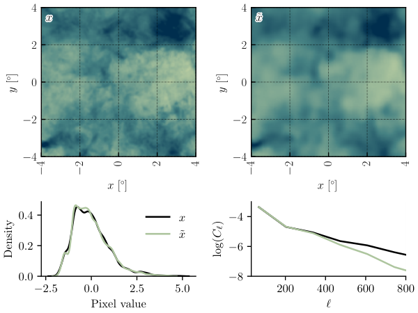
In Figure 2 we take a single randomly-selected test set image, and show its reconstruction, the pixel value histograms of each image, and their power spectra. As was the case for the three examples shown in Figure 1, there is excellent visual agreement between the original image and its reconstruction. This is enforced by the excellent agreement between the distribution of pixel values in the two images, shown in the bottom left panel of Figure 2. The reconstructed power spectrum in the bottom right panel of Figure 2 also shows excellent agreement up to $\ell\sim 400$, and suppression of power in the reconstructed image going to smaller scales, consistent with the visual blurriness of the reconstructed image.

In order to compare reconstructions for the whole test set, we now calculate the pixel value distribution and power spectrum for each of the 339 images in the test set and their reconstructions. In order to represent the distribution of pixel value histograms across this test set, we calculate the quartiles and median in each bin, across the test set. In Figure 3 we plot the $25^{\rm th}$ percentile, median, and $75^{\rm th}$ percentile as a function of bin center, for both the original test set images, and their reconstructions. There is excellent agreement between the two sets of images, with no evidence of any aggregate bias in the reconstructions.

In Figure 4 we compare the power spectra of all test set images and their reconstructions. Figure 4 shows that the same behavior as was seen in Figure 2 is displayed for the entire test set. Spectra are generally well recovered for $\ell<400$, with power being increasingly suppressed for $\ell>400$, relative to the real image power spectra.

Here, we are encountering a known issue with VAEs: reconstructed images are often blurry (Kingma & Dhariwal 2018; Kingma et al. 2016; Kingma & Welling 2019). The blurriness can be understood by considering the objective function in Equation 7, and inspecting the term $\mathbb{E}_{q_{\phi}(\mathbf{z}|\mathbf{x})}\left[p_{\theta}(\mathbf{x},\mathbf{z})\right]$. Since this expectation is taken with respect to the distribution $q_{\phi}(\mathbf{z}|\mathbf{x})$, it will strongly penalize points $(\mathbf{x},\mathbf{z})$ that are likely under $q_{\phi}$, but unlikely under $p_{\theta}$. On the other hand, points that are likely under $p_{\theta}$, but are not present in the empirical data distribution, will suffer a much smaller penalty. The result is that, if the model is not sufficiently flexible to fit the data distribution exactly, it will compensate by widening the support of $p_{\theta}(\mathbf{x},\mathbf{z})$ beyond what is present in the data distribution, inflating the variance of $p_{\theta}(\mathbf{x}|\mathbf{z})$. Since we have assumed a Gaussian distribution for the decoder model that is independent from pixel to pixel, and given that the signal in the training images is red-tilted (as is the case for most natural images containing extended recognizable structures), the increased variance leads to a degradation of small-scale features through the averaging process of Equation 10 (Zhao et al. 2017). A corollary of the extended support of $p_{\theta}(\mathbf{x},\mathbf{z})$ is that sampling the prior in order to generate novel images will not necessarily produce realistic samples (Kingma & Welling 2019).

One way in which the flexibility of VAEs may be enhanced is through the use of normalizing flows (Jimenez Rezende & Mohamed 2015). As the name suggests, the idea here is to start with a simple distribution, such as a multivariate normal, and ‘stack’ layers of invertible transformations, such that the output may be significantly more complex. There are certain requirements placed on these transformations such that they remain computationally efficient, for example they must have tractable Jacobians (Jimenez Rezende & Mohamed 2015). Expanding the VAE model presented here by introducing normalizing flows could be expected to improve both the reconstruction quality, and the quality of novel samples, and is the subject of current work.

As a means of investigating the structure of the encoding that has been learned, we study the ‘interpolation’ between real images, $\mathbf{x}_{1}$ and $\mathbf{x}_{2}$, by performing the interpolation between their latent encodings, $\mathbf{z}_{1}$ and , $\mathbf{z}_{2}$. From the smooth nature of the changes in the resulting continuum of maps we will see that smooth variations in the latent space result in smooth variations in the map space. This study also demonstrates the ability of the VAE approach to generate novel foreground images by restricting to a region of the latent space close to the encodings of real maps, therefore avoiding the spurious regions of $(\mathbf{x},\mathbf{z})$ that could be obtained by sampling from an ill-fitted prior, as discussed at the end of Section 3.1.

The probability mass in high-dimensional distributions tends to concentrate in a shell relatively far from the modal probability density. Therefore, traversing the latent space in a straight line (in the Euclidean sense), does not necessarily pass through areas of high probability mass. In order to keep the interpolated points within areas of high probability mass, we interpolate from $\mathbf{z}_{1}$ to $\mathbf{z}_{2}$ using spherical trajectories that traverse great circles in the latent space, as the distance from the origin smoothly changes from $|\mathbf{z_{1}}|$ to $|\mathbf{z_{2}}|$. Specifically, we follow this continuous trajectory parametrized by some factor $\lambda$:

where $\cos(\theta)=\hat{\mathbf{z}}_{1}\cdot\hat{\mathbf{z}}_{2}$. We then take $N$ points along this line corresponding to $\lambda=[1/(N+1),2/(N+1),\dots,N/(N+1)]$, and decode to obtain the corresponding map $\mathbf{x}_{1,2}(\lambda)=g_{\phi}(\mathbf{z}_{1,2}(\lambda))$.

Figure 5 shows the smooth transition in image space between the two real images (the top left panel and the bottom right panel) randomly selected from the test set, calculated using the interpolation described above. Features, such as the strong filamentary structures in the center of the image, transition smoothly in and out of the image, demonstrating that small perturbations in the latent space result in small perturbations in decoded images.

In this section we consider a possible application of our trained model to the reconstruction of corrupted data. During the analysis of CMB data there are many possible reasons that data may be incomplete, from masking of point sources, to corruption by uncontrolled systematics. The task of inpainting these regions is simple when the missing emission is well described by Gaussian statistics, as is the case for the CMB (Bucher & Louis 2012). The lack of a similarly simple approach for the non-Gaussian foreground signal means that previous efforts have relied on empirically-validated, simple, algorithms, such as diffusive filling (Bucher et al. 2016). Future surveys will have ever-lower noise floors, and so will be increasingly contaminated by point-sources, even in polarization. The aggressive masking required in this regime could lead to the failure of simple foreground inpainting techniques (Puglisi & Bai 2020). The statistical foreground model presented here allows us to take a Bayesian approach to foreground inpainting, in which we may compute a posterior distribution for the missing data, conditioned on the observed data (Böhm et al. 2019). This has the advantage of conserving the foregrounds’ statistical properties, whilst also taking into account all of the contextual information in the image, unlike methods such as diffusive inpainting. In the rest of this section we will present a toy model for corrupted data, and show that we are able to perform inpainting by optimizing the posterior distribution in the latent space.

Representing the contamination as a linear operator $\mathsf{A}$, we can write down a model for the observed data $\mathbf{d}$: $\mathbf{d}=\mathsf{A}\mathbf{x}+\mathbf{n}$, where $\mathbf{n}$ is a possible noise term. The posterior distribution of $\mathbf{z}$ is given by Bayes’ theorem:

For a given statistical model of the noise, we have a complete description of the term $\log p(\mathbf{d}|\mathbf{z})$, and we can work with the posterior distribution in the latent space.

As a concrete example we will consider the case of a binary $N\times N$ masking operator, $\mathsf{A}$, with elements equal to one (zero) where pixels are (un)observed. To form simulated ‘corrupted’ images, we take random images from the test dataset, apply $\mathsf{A}$, and add white Gaussian noise $\mathbf{n}$, characterized by a pixel standard deviation $\sigma$: $\mathbf{d}_{\rm test}=\mathsf{A}\mathbf{x}_{\rm test}+\mathbf{n}$. The posterior distribution in the latent space is then:

where we have written the residual vector as $\bm{\mu}_{\theta}(\mathbf{z})=\mathsf{A}\mathbf{g}_{\theta}(\mathbf{z})-\mathbf{d}_{\rm test}$.

Fully sampling Equation 13 can be computationally expensive due to the dimensionality of $\mathbf{z}$, and is made more challenging by the possibility of $\log p(\mathbf{z}|\mathbf{d}_{\rm test})$ being multi-modal. For these reasons, applying standard Markov Chain Monte Carlo techniques can often fail to fully explore the posterior (Böhm et al. 2019), and we leave a sampling approach for future work, here taking only a single representative sample by maximizing $\hat{\mathbf{z}}_{\rm test}=\argmax_{\mathbf{z}}\log p(\mathbf{z}|\mathbf{d}_{\rm test})$.

In the following we will take $\mathsf{A}$ to be a masking operator that applies a binary mask to a map. However, as long as a forward model for the corruption operation can be written down (e.g. a Gaussian convolution), the same technique could be applied. We take three randomly selected test set images, $\mathbf{x}_{1},\mathbf{x}_{2},\mathbf{x}_{3}$, and apply three different binary masks, $\mathsf{A}_{1},\mathsf{A}_{2},\mathsf{A}_{3}$. To each corrupted image, we add a white noise realization with a pixel standard deviation of 0.2. For each corrupted, noisy image, we then maximize the posterior in Equation 13 to find $\mathbf{z}_{i}^{\rm MAP}$ using the LBFGS algorithm. In Figure 6 we show the randomly selected test set images in the first row, the corrupted images in the second row, and the reconstructed map $g(\mathbf{z}_{i}^{\rm MAP})$ in the third row. We also calculate the pixel value histograms and power spectra of the input and reconstructed maps and show these in the bottom two rows of Figure 6.

One can see from Figure 6 that all the images are well reconstructed, and there is no visible effect of the masking remaining in the reconstructions. Comparing the regions in the first and third rows corresponding to the masked areas, we see that the network does not reproduce the exact features in the masked region, for any of the $\mathbf{x}_{i}$, as expected. However, the network does reconstruct plausible inpaintings, with the correct statistics, given the context in the rest of the image. For example, the reconstruction $g_{\phi}(\mathbf{z}_{2}^{\rm MAP})$ does not replicate the true high-intensity filamentary structure in the input image, $\mathbf{x}_{2}$, which would be impossible. However, it does recognize from the context that intensity is increasing towards the masked area in the bottom left of the image, and populates that area with high-variance, high-intensity features. Correspondingly, such high-intensity features are not seen in the reconstructed regions of $g_{\phi}(\mathbf{z}_{1,3}^{\rm MAP})$, which correspond to relatively low-emission regions. The pixel value histograms and power spectra in the last two rows of Figure 6 show similar behavior. We see good agreement between the original and reconstructed histograms and powerspectra for both the $\mathbf{x}_{1}$ and $\mathbf{x}_{3}$ maps, up to the suppression at $\ell>400$ common to all reconstructions. On the other hand, we see a disagreement between the original and reconstructed statistics of $\mathbf{x}_{2}$, due to the higher variance associated with the filled-in region.

These results show that the network has learned generalizable information about foreground behavior, and is able to inpaint novel foreground emission with correct statistical properties, based on the context of an image. The forward model used in this inpainting process can be easily extended to maps with multiple masks and different types of filtering and noise found in real data.

References

- Abadi et al. (2015) Abadi M., et al., 2015, TensorFlow: Large-Scale Machine Learning on Heterogeneous Systems, https://www.tensorflow.org/
- Ade et al. (2019) Ade P., et al., 2019, J. Cosmology Astropart. Phys., 2019, 056
- Aiola et al. (2020) Aiola S., et al., 2020, arXiv e-prints, p. arXiv:2007.07288
- Alonso et al. (2019) Alonso D., Sanchez J., Slosar A., LSST Dark Energy Science Collaboration 2019, MNRAS, 484, 4127
- Aylor et al. (2019) Aylor K., Haq M., Knox L., Hezaveh Y., Perreault-Levasseur L., 2019, arXiv e-prints, p. arXiv:1909.06467
- BICEP2 Collaboration et al. (2018) BICEP2 Collaboration et al., 2018, Phys. Rev. Lett., 121, 221301
- Benson et al. (2014) Benson B. A., et al., 2014, in Holland W. S., Zmuidzinas J., eds, Vol. 9153, Millimeter, Submillimeter, and Far-Infrared Detectors and Instrumentation for Astronomy VII. SPIE, pp 552 – 572, doi:10.1117/12.2057305, https://doi.org/10.1117/12.2057305
- Böhm et al. (2019) Böhm V., Lanusse F., Seljak U., 2019, arXiv e-prints, p. arXiv:1910.10046
- Brock et al. (2018) Brock A., Donahue J., Simonyan K., 2018, arXiv e-prints, p. arXiv:1809.11096
- Bucher & Louis (2012) Bucher M., Louis T., 2012, MNRAS, 424, 1694
- Bucher et al. (2016) Bucher M., Racine B., van Tent B., 2016, Journal of Cosmology and Astroparticle Physics, 2016, 055
- Dinh et al. (2014) Dinh L., Krueger D., Bengio Y., 2014, arXiv e-prints, p. arXiv:1410.8516
- Dinh et al. (2016) Dinh L., Sohl-Dickstein J., Bengio S., 2016, arXiv e-prints, p. arXiv:1605.08803
- Goodfellow et al. (2014) Goodfellow I. J., Pouget-Abadie J., Mirza M., Xu B., Warde-Farley D., Ozair S., Courville A., Bengio Y., 2014, arXiv e-prints, p. arXiv:1406.2661
- Goodfellow et al. (2016) Goodfellow I., Bengio Y., Courville A., 2016, Deep Learning. MIT Press
- Grover et al. (2017) Grover A., Dhar M., Ermon S., 2017, arXiv e-prints, p. arXiv:1705.08868
- Hui et al. (2018) Hui H., et al., 2018, in Zmuidzinas J., Gao J.-R., eds, Society of Photo-Optical Instrumentation Engineers (SPIE) Conference Series Vol. 10708, Millimeter, Submillimeter, and Far-Infrared Detectors and Instrumentation for Astronomy IX. p. 1070807 (arXiv:1808.00568), doi:10.1117/12.2311725
- Jimenez Rezende & Mohamed (2015) Jimenez Rezende D., Mohamed S., 2015, arXiv e-prints, p. arXiv:1505.05770
- Jimenez Rezende et al. (2014) Jimenez Rezende D., Mohamed S., Wierstra D., 2014, arXiv e-prints, p. arXiv:1401.4082
- Kamionkowski et al. (1997) Kamionkowski M., Kosowsky A., Stebbins A., 1997, Phys. Rev. Lett., 78, 2058
- Kim et al. (2019) Kim C.-G., Choi S. K., Flauger R., 2019, ApJ, 880, 106
- Kingma & Dhariwal (2018) Kingma D. P., Dhariwal P., 2018, arXiv e-prints, p. arXiv:1807.03039
- Kingma & Welling (2013) Kingma D. P., Welling M., 2013, arXiv e-prints, p. arXiv:1312.6114
- Kingma & Welling (2019) Kingma D. P., Welling M., 2019, arXiv e-prints, p. arXiv:1906.02691
- Kingma et al. (2016) Kingma D. P., Salimans T., Jozefowicz R., Chen X., Sutskever I., Welling M., 2016, arXiv e-prints, p. arXiv:1606.04934
- Knox & Turner (1994) Knox L., Turner M. S., 1994, Phys. Rev. Lett., 73, 3347
- Krachmalnicoff & Puglisi (2020) Krachmalnicoff N., Puglisi G., 2020, arXiv e-prints, p. arXiv:2011.02221
- Krachmalnicoff & Tomasi (2019) Krachmalnicoff N., Tomasi M., 2019, A&A, 628, A129
- Millea et al. (2020a) Millea M., Anderes E., Wandelt B. D., 2020a, arXiv e-prints, p. arXiv:2002.00965
- Millea et al. (2020b) Millea M., et al., 2020b, arXiv e-prints, p. arXiv:2012.01709
- Perraudin et al. (2019) Perraudin N., Defferrard M., Kacprzak T., Sgier R., 2019, Astronomy and Computing, 27, 130
- Petroff et al. (2020) Petroff M. A., Addison G. E., Bennett C. L., Weiland J. L., 2020, arXiv e-prints, p. arXiv:2004.11507
- Planck Collaboration et al. (2020) Planck Collaboration et al., 2020, A&A, 641, A6
- Puglisi & Bai (2020) Puglisi G., Bai X., 2020, arXiv e-prints, p. arXiv:2003.13691
- Razavi et al. (2019) Razavi A., van den Oord A., Vinyals O., 2019, arXiv e-prints, p. arXiv:1906.00446
- Russakovsky et al. (2015) Russakovsky O., et al., 2015, International Journal of Computer Vision (IJCV), 115, 211
- Seljak & Zaldarriaga (1997) Seljak U., Zaldarriaga M., 1997, Phys. Rev. Lett., 78, 2054
- Smoot et al. (1992) Smoot G. F., et al., 1992, ApJ, 396, L1
- Zhao et al. (2017) Zhao S., Song J., Ermon S., 2017, arXiv e-prints, p. arXiv:1702.08658
- van den Oord et al. (2016a) van den Oord A., Kalchbrenner N., Kavukcuoglu K., 2016a, arXiv e-prints, p. arXiv:1601.06759
- van den Oord et al. (2016b) van den Oord A., et al., 2016b, arXiv e-prints, p. arXiv:1609.03499