Blind Reconstruction of Multilayered Tissue Profiles with UWB Radar Under Bayesian Setting

We consider an UWB system where we transmit a short duration UWB pulse and collect the backscattered signals which are reflections from an object composed of multiple planar layers. The layers are assumed to be homogeneous mediums and have distinct dielectric properties such that the interfaces between them can be considered as reflective surfaces. The backscattered signal can be expressed as a combination of scaled, shifted and distorted versions of the transmitted waveform. The distortion occurs due to materials either being dispersive or having non-zero conductivity. These factors are completely determined by the reflectivity profile of the target being monitored. In general, for an $M$-layer structure with thicknesses $d_{i}$, as illustrated in Fig. 1, where the last layer has infinite depth, the 1D downward reflectivity profile $X_{i}(\omega)$ in frequency domain has the following recursive form [25]

at each interface $I_{i}$ for $i=1,\ldots,M-1$, with $X_{M}(\omega)=r_{M}$ and $\omega$ representing the angular frequency in rad/sec. The downward local reflection coefficient at interface $I_{i}$ is given by $r_{i}=(\eta_{i}-\eta_{i-1})/(\eta_{i}+\eta_{i-1})$, where $\eta_{i}=\sqrt{(j\omega\mu_{o})/(\sigma_{i}+j\omega\varepsilon_{o}\varepsilon_{i})}$ is the complex valued intrinsic impedance defined in terms of the dielectric constant $\varepsilon_{i}$ and conductivity $\sigma_{i}$ in S/m of the mediums. Here, $\mu_{o}$ and $\varepsilon_{o}$ are constants representing the vacuum permeability in H/m and vacuum permittivity in F/m respectively. Lastly, $\alpha_{i}=\omega[\mu_{o}\varepsilon_{o}\varepsilon_{i}(\zeta_{i}-1)/2]^{1/2}$ and $\beta_{i}=\omega[\mu_{o}\varepsilon_{o}\varepsilon_{i}(\zeta_{i}+1)/2]^{1/2}$ represent the attenuation coefficients and the phase constants respectively, where $\zeta_{i}=\sqrt{1+(\sigma_{i}/\omega\varepsilon_{o}\varepsilon_{i})^{2}}$.

In this work, we consider the scenario in which the source of the transmitted pulse is $d_{0}$ meters away from the interface $I_{1}$ with normal incidence. Therefore, for a given frequency $\omega$, the corresponding frequency component of the transmitted pulse, $H(\omega)$, is multiplied by $X_{0}(\omega)=X_{1}(\omega)e^{-2\alpha_{0}d_{0}}e^{-j2\beta_{0}d_{0}}$, yielding the following backscattering model $Y(\omega)=H(\omega)X_{0}(\omega)$, where $Y(\omega)$ represents the frequency domain representation of the backscattered signal. In practice, we observe the measurement sampled at frequencies $\{\omega_{n}\}_{n=0}^{N-1}$, which can be modeled as

where $\mbox{\boldmath${y}$},\mbox{\boldmath${x}$}\in\mathbbm{C}^{N}$ are defined as $\mbox{\boldmath${y}$}=[Y(\omega_{0}),\ldots,Y(\omega_{N-1})]^{T}$ and $\mbox{\boldmath${x}$}=[X_{0}(\omega_{0}),\ldots,X_{0}(\omega_{N-1})]^{T}$, and the transmitted waveform is modeled in time domain as $\mbox{\boldmath${h}$}\in\mathbbm{R}^{Q}$ to limit its duration with $Q$ samples in time domain. The matrix $\mbox{\boldmath${F}$}_{Q}\in\mathbbm{C}^{N\times Q}$ represents the appropriately selected partial DFT matrix. We model the measurement noise by including a complex valued additive noise term $\mbox{\boldmath${v}$}\in\mathbbm{C}^{N}$.

Consider a high dimensional target probability distribution $\pi(\mbox{\boldmath${z}$})$, from which we aim to draw samples. When the target distribution $\pi(\mbox{\boldmath${z}$})$ is highly multimodal, the standard MCMC samplers such as MH and Gibbs, or even more sophisticated methods like HMC, fail to explore the probability space efficiently, due to the low probability regions acting like barriers in between the modes of the distribution. The main idea of tempering is to augment the original target distribution $\pi(\mbox{\boldmath${z}$})$ with an additional temperature variable $T$ to create the tempered distribution $\pi(\mbox{\boldmath${z}$};T)=K(T)\pi(\mbox{\boldmath${z}$})^{1/T}$, where $K(T)$ denotes the normalization constant. As illustrated in Fig. 2, tempering, when $T>1$, has a flattening effect on the original distribution, which removes the low probability barriers between the modes. Therefore, jumps between different modes become much more likely for the distributions with high temperatures.

The idea of Parallel Tempering (PT) is to run multiple MCMC chains independently and simultaneously at each temperature level with stochastic temperature swaps between the neighbouring temperature levels [27]. The target distribution in PT is a joint distribution over all chains given by $\prod_{\ell=1}^{L}\pi(\mbox{\boldmath${z}$}^{(\ell)};T_{\ell})$, where $\mbox{\boldmath${z}$}^{(\ell)}$ denotes the variables for the chain running at temperature level $T_{\ell}$. Assuming symmetric proposals, the acceptance probability $\alpha_{\ell,\ell+1}$ that maintains the detailed balance in the case of a temperature swap between the chains at $T_{\ell}$ and $T_{\ell+1}$ is given by

We begin with introducing the general structure of our proposed sampler and discussing its connection to the Parallel Tempering approach. We employ a Gibbs sampler scheme, which is a powerful MCMC tool for sampling from high dimensional distributions especially when the conditional posteriors are analytically tractable and straightforward to sample from [28]. Here, note that the multimodality of the posterior is mainly due to the likelihood function given in (4). The prior distributions assigned to the pulse shape and the noise variance do not contribute to the multimodality of the target posterior. Therefore, we follow an alternative tempering approach, where we partially temper the posterior distribution by applying tempering only to the likelihood. With this approach, the chains running at high temperatures will sample from the prior distributions, instead of a flat distribution over the parameter space. This is quite useful when the prior distributions are unimodal, which is the case for the Gaussian and Inverse-Gamma distributions.

One iteration of the proposed Gibbs sampler for sampling from the partially tempered posterior $p(\mbox{\boldmath${\theta}$},\mbox{\boldmath${\gamma}$},\sigma_{v}^{2}|\mbox{\boldmath${y}$};T)\propto p(\mbox{\boldmath${y}$}|\mbox{\boldmath${\theta}$},\mbox{\boldmath${\gamma}$},\sigma_{v}^{2})^{1/T}p(\mbox{\boldmath${\theta}$},\mbox{\boldmath${\gamma}$},\sigma_{v}^{2})$ for a given temperature $T$ is given in Table I. This is a valid Gibbs sampler, which samples each variable at least once within one iteration. The validity of the sampler is established in Section I of the supplementary material by showing that the MH acceptance probability is always 1 for each step. Here, due to our selection of conjugate priors for $\sigma_{v}^{2}$ and ${\gamma}$, the partially tempered posterior conditionals $p(\sigma_{v}^{2}|\mbox{\boldmath${y}$},\mbox{\boldmath${\theta}$},\mbox{\boldmath${\gamma}$};T)\propto p(\mbox{\boldmath${y}$}|\mbox{\boldmath${\theta}$},\mbox{\boldmath${\gamma}$},\sigma_{v}^{2})^{1/T}p(\sigma_{v}^{2})$ and $p(\mbox{\boldmath${\gamma}$}|\mbox{\boldmath${y}$},\mbox{\boldmath${\theta}$},\sigma_{v}^{2};T)\propto p(\mbox{\boldmath${y}$}|\mbox{\boldmath${\theta}$},\mbox{\boldmath${\gamma}$},\sigma_{v}^{2})^{1/T}p(\mbox{\boldmath${\gamma}$})$ in Steps 1 and 2 have well-known forms in which the sampling is straightforward. However, the posterior conditional of the multilayer model parameters $p(\mbox{\boldmath${\theta}$}|\mbox{\boldmath${y}$},\mbox{\boldmath${\gamma}$},\sigma_{v}^{2};T)\propto p(\mbox{\boldmath${y}$}|\mbox{\boldmath${\theta}$},\mbox{\boldmath${\gamma}$},\sigma_{v}^{2})^{1/T}p(\mbox{\boldmath${\theta}$})$, given in Step 3, is highly complex and does not have a well-known form, which prevents direct sampling of ${\theta}$. Therefore, we will create a hierarchical sampling scheme and propose a hybrid sampling mechanism combining Slice Sampling and Hamiltonian Monte Carlo approaches, to draw samples from $p(\mbox{\boldmath${\theta}$}|\mbox{\boldmath${y}$},\mbox{\boldmath${\gamma}$},\sigma_{v}^{2};T)$. We present the details of the proposed hybrid sampling method in Section V. We now describe how the Parallel Tempering approach is incorporated with the proposed Gibbs sampler, followed by the derivation of sampling distributions for Steps 1 and 2.

Considering a Parallel Tempering scheme with $L$ temperature levels, each MCMC chain samples from a specific partially tempered version of the posterior distribution, i.e., the chain at level $T_{\ell}$ samples from $p(\mbox{\boldmath${\theta}$},\mbox{\boldmath${\gamma}$},\sigma_{v}^{2}|\mbox{\boldmath${y}$};T_{\ell})\propto p(\mbox{\boldmath${y}$}|\mbox{\boldmath${\theta}$},\mbox{\boldmath${\gamma}$},\sigma_{v}^{2})^{1/T_{\ell}}p(\mbox{\boldmath${\theta}$},\mbox{\boldmath${\gamma}$},\sigma_{v}^{2})$ for $\ell=1,2,\ldots,L$. After one iteration of the Gibbs sampler is completed at all chains, a parameter exchange between the neighbouring levels, say, $T_{\ell}$ and $T_{\ell+1}$, is proposed, where $\ell$ is randomly selected from the uniformly distributed proposal distribution $q_{\ell}=1/(L-1)$ for $\ell\in\{1,2,\ldots,L-1\}$. The proposal is accepted with the following acceptance probability

where $(\mbox{\boldmath${\theta}$}^{(\ell,j)},\mbox{\boldmath${\gamma}$}^{(\ell,j)},\sigma_{v}^{2(\ell,j)})$ and $(\mbox{\boldmath${\theta}$}^{(\ell+1,j)},\mbox{\boldmath${\gamma}$}^{(\ell+1,j)},\sigma_{v}^{2(\ell+1,j)})$ represent the current parameter values at $j^{th}$ MCMC iteration which are to be exchanged between the chains running at level $T_{\ell}$ and $T_{\ell+1}$ respectively (See Section II of the supplementary material for derivation of the acceptance probability). Therefore, one complete MCMC cycle consists of $L$ regular Gibbs sampling stages, followed by a single parameter exchange step. Each cycle $j$ produces a new set of samples for each temperature level, $\{(\mbox{\boldmath${\theta}$}^{(\ell,j)},\mbox{\boldmath${\gamma}$}^{(\ell,j)},\sigma_{v}^{2(\ell,j)})\}_{\ell=1}^{L}$, but in the end, we are only interested in the samples generated at the first level, $T_{1}=1$, which corresponds to the original posterior distribution. We provide a more detailed description of the sampler in Algorithm 1. Next, we present the sampling distributions for the first two steps of our sampler, associated with each temperature level. The derivations are provided in Section III of the supplementary material.

SS is among the widely used methods for within-Gibbs sampling schemes [29]. It is applicable to both univariate and multivariate cases when the target distribution can be calculated up to a scale. In this work, we employ the univariate setting and sample ${\theta}$ in $3M$ steps, where in each step, we sample an element $\theta_{i}$ from its full conditional posterior distribution $p(\theta_{i}|\mbox{\boldmath${y}$},\mbox{\boldmath${\theta}$}_{-i},\mbox{\boldmath${\gamma}$},\sigma_{v}^{2};T)$, associated with a given temperature level $T$. The first step of SS is to randomly draw a density level $\eta_{i}$ from $U[0,p(\theta_{i}|\mbox{\boldmath${y}$},\mbox{\boldmath${\theta}$}_{-i},\mbox{\boldmath${\gamma}$},\sigma_{v}^{2};T)]$. Then, a line segment (or a hyper-rectangle for multivariate case) with predefined length, $w_{i}$, is randomly positioned around $\theta_{i}$ and sequentially extended in both directions with multiples of $w_{i}$ until both ends are above $p(\theta_{i}|\mbox{\boldmath${y}$},\mbox{\boldmath${\theta}$}_{-i},\mbox{\boldmath${\gamma}$},\sigma_{v}^{2};T)$, which is known as the stepping-out procedure. Once the stepping-out procedure is completed, a point $\tilde{\theta}_{i}$ is drawn uniformly within the extended line segment. If the selected point does not satisfy $p(\tilde{\theta}_{i}|\mbox{\boldmath${y}$},\mbox{\boldmath${\theta}$}_{-i},\mbox{\boldmath${\gamma}$},\sigma_{v}^{2};T)\geq\eta_{i}$, the line segment is shrunk by setting one end to $\tilde{\theta}_{i}$ such that $\theta_{i}$ still lies within the resulting line segment and a new point is drawn randomly in the same manner. The shrinkage process, also known as stepping-in procedure, continues until a point satisfies $p(\tilde{\theta}_{i}|\mbox{\boldmath${y}$},\mbox{\boldmath${\theta}$}_{-i},\mbox{\boldmath${\gamma}$},\sigma_{v}^{2};T)\geq\eta_{i}$. Once such a point is selected, it is assigned as the next sample value. Throughout this work, we set the length of line segment as the range of corresponding parameter, i.e., $w_{i}=\theta_{i,\text{max}}-\theta_{i,\text{min}}$.

The core idea of HMC is to utilize the geometry of the target distribution to eliminate the random walk behaviour of the conventional Metropolis-Hastings (MH) method by enabling longer jumps in parameter space with high acceptance rate [30]. It is based on an analogy with physical systems, in which the target distribution is translated to a potential energy function, where the parameters of interest, ${\theta}$, are regarded as position variables. An augmented state-space is created by introducing momentum variables, denoted by ${p}$, representing the rate of change of the position variables. Defining the tempered potential energy function as $U(\mbox{\boldmath${\theta}$};T)=-\log p(\mbox{\boldmath${y}$}|\mbox{\boldmath${\theta}$},\mbox{\boldmath${\gamma}$},\sigma_{v}^{2};T)$ and the kinetic energy function as $K(\mbox{\boldmath${p}$})=\frac{1}{2}\mbox{\boldmath${p}$}^{T}\mbox{\boldmath${M}$}\mbox{\boldmath${p}$}$, where ${M}$ is a weighting matrix that adjusts the momentum distribution for more efficient sampling, total energy of the system at a given state $(\mbox{\boldmath${\theta}$},\mbox{\boldmath${p}$})$ at temperature $T$ is given by the Hamiltonian $H(\mbox{\boldmath${\theta}$},\mbox{\boldmath${p}$};T)=U(\mbox{\boldmath${\theta}$};T)+K(\mbox{\boldmath${p}$})$.

HMC is used to sample $(\mbox{\boldmath${\theta}$},\mbox{\boldmath${p}$})$ pairs jointly from the canonical distribution $P(\mbox{\boldmath${\theta}$},\mbox{\boldmath${p}$};T)\propto\exp\big(-H(\mbox{\boldmath${\theta}$},\mbox{\boldmath${p}$};T)\big)$ at a given temperature level $T$. The sampling is achieved by first sampling a new momentum state from $\mathcal{N}(\mbox{\boldmath${p}$};\mbox{\boldmath${0}$},\mbox{\boldmath${M}$}^{-1})$, and then simulating the Hamiltonian dynamics, given by

to produce a new position state. However, exact simulation requires integration of (9), which is not feasible in practice. Hence, it is approximated by the leapfrog algorithm, which is a numerical integration scheme consisting of alternating discretized updates to ${\theta}$ and ${p}$: $i)$ $\mbox{\boldmath${p}$}_{\epsilon/2}=\mbox{\boldmath${p}$}_{0}-\frac{\epsilon}{2}\nabla_{\theta}U(\mbox{\boldmath${\theta}$}_{0};T)$, $ii)$ $\mbox{\boldmath${\theta}$}_{\epsilon}=\mbox{\boldmath${\theta}$}_{0}+\epsilon\mbox{\boldmath${M}$}\mbox{\boldmath${p}$}_{\epsilon/2}$, and $iii)$ $\mbox{\boldmath${p}$}_{\epsilon}=\mbox{\boldmath${p}$}_{\epsilon/2}-\frac{\epsilon}{2}\nabla_{\theta}U(\mbox{\boldmath${\theta}$}_{\epsilon};T)$.

One iteration of the leapfrog algorithm simulates the dynamics for a time interval $\epsilon$, which is the predefined step size of the algorithm. In order to simulate for a duration of $\tau$, the process is repeated for $\Delta=\tau/\epsilon$ times. Although the leapfrog algorithm provides quite accurate approximation of the continuous time integration, some residual error will remain due to discretization, which might alter the value of Hamiltonian. In order to maintain detailed balance, the proposed state is accepted with MH acceptance criterion.

HMC is conventionally used for sampling from smooth and unbounded distributions. For bounded parameter spaces, as we have with $\Lambda_{\theta}$, a modified reflective HMC can be used, where the trajectory on the parameter space is bounced back when it is blocked by a boundary. Specifically, if $\theta_{i}\notin[\theta_{i,\text{min}},\theta_{i,\text{max}}]$ after completing one step of the leapfrog algorithm, we undo the previous step, negate the $i^{th}$ momentum variable, i.e., $p_{i}^{\prime}=-p_{i}$, and then complete the remaining steps using the updated momentum vector. If multiple boundaries are violated simultaneously, all of the corresponding momentum variables are negated. In Fig. 3, we demonstrate the employed reflection method for a two-dimensional case. This method of reflection leaves the Hamiltonian invariant, since negation does not change the value of kinetic energy function, i.e., $K(\mbox{\boldmath${p}$}^{\prime})=K(\mbox{\boldmath${p}$})$. Moreover, the same MH acceptance criterion remains valid, preserving the detailed balance.

Note that the leapfrog algorithm still requires the analytic expression for the gradient of the potential energy function $U(\mbox{\boldmath${\theta}$};T)=\|\mbox{\boldmath${y}$}-\text{diag}(\mbox{\boldmath${B}$}\mbox{\boldmath${\gamma}$})\mbox{\boldmath${x}$}\|^{2}/T\sigma_{v}^{2}$. Following the derivation provided in Section IV of the supplementary material, it is given by

where $\mbox{\boldmath${D}$}=\text{diag}(\mbox{\boldmath${B}$}\mbox{\boldmath${\gamma}$})$. The gradient of ${x}$ is defined as $\nabla_{\theta}\mbox{\boldmath${x}$}=[\nabla_{\theta}X_{0}(\omega_{0}),\nabla_{\theta}X_{0}(\omega_{1}),\ldots,\nabla_{\theta}X_{0}(\omega_{N-1})]^{T}$, where the individual terms $\nabla_{\theta}X_{0}(\omega_{i})$ have the form of $\nabla_{\theta}X_{0}(\omega_{i})=[\partial X_{0}(\omega_{i})/\partial\theta_{1},\ldots,\partial X_{0}(\omega_{i})/\partial\theta_{3M}]^{T}$ for $i=0,1,\ldots,N-1$. Exact expression for each element of $\nabla_{\theta}X_{0}(\omega_{i})$ is also provided in Section IV of the supplementary material.

The parameters $\epsilon$, $\Delta$ and ${M}$ affect the overall performance of HMC significantly. In general, higher $\epsilon$ causes high residual error leading to low acceptance rate. On the other hand, selecting a too small $\epsilon$ will require large number of steps $\Delta$ to achieve long jumps, which increases the computational load. Hence, both parameters need to be tuned for the best trade-off. Similarly, appropriate selection of ${M}$ is crucial for sampling efficiency. Note that the residual error is actually the sum of all errors in each dimensions. Therefore, the simple choice of $\mbox{\boldmath${M}$}=\mbox{\boldmath${I}$}$, which assigns equal weights for all dimensions, causes step size $\epsilon$ to be determined according to the dimension with the smallest variance. This is because a smaller variance at a given direction generally corresponds to a higher gradient in that direction, which increases sensitivity to the value of the momentum. The performance can be significantly improved by adjusting the momentum variables accordingly to maintain a similar level of error in each dimension. This can be achieved by selecting ${M}$ as a diagonal matrix consisting of the inverse of the variances in each dimension. A better strategy would be to set ${M}$ as the inverse of the full covariance matrix ${\Sigma}$, which would not only incorporate the variance information, but also capture the linear correlations between the parameters. However, for complex distributions, analytical calculation of the covariance matrix is not possible, and hence, an estimate is required. In addition to these issues, another essential but non-trivial problem is the selection of the temperature ladder for PT scheme as it has a substantial effect on the overall exploration power of the sampler. Since no unique set of temperature levels exist that works well for all distributions, the temperatures should be adjusted for improved sampling performance.

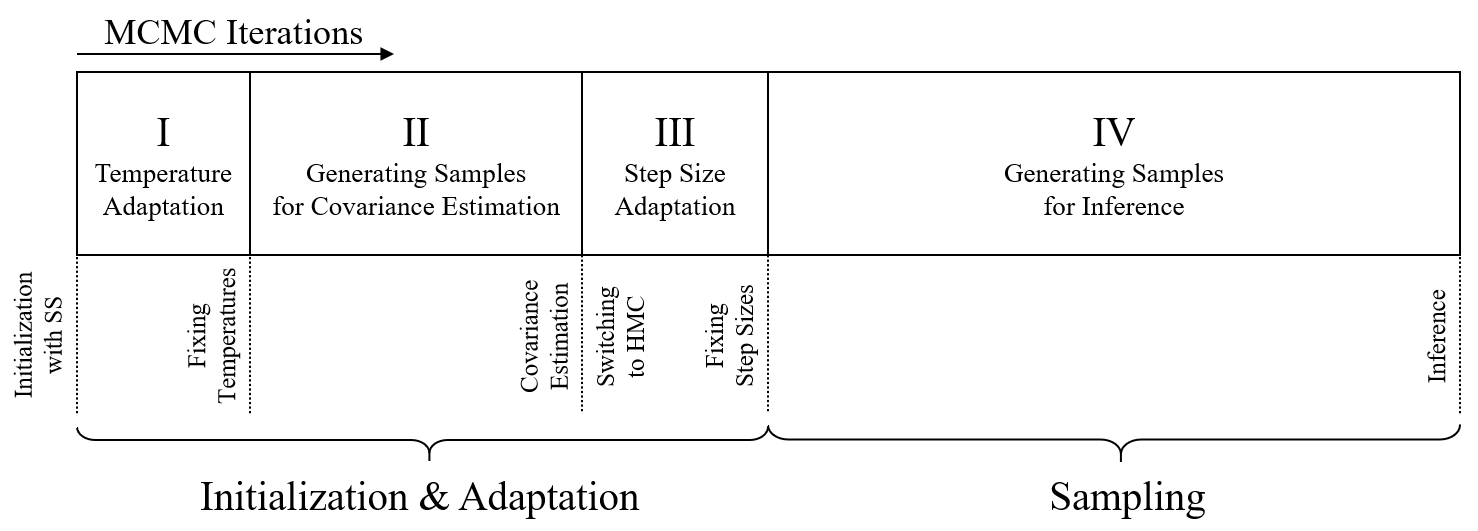
To address the issues described above, we designed an adaptive sampling mechanism that consists of an initialization/adaptation stage as part of the burn-in process for learning the temperature levels as well as the covariance matrices and the step sizes (for fixed number of steps $\Delta$) associated with each temperature level from the measurement. As illustrated in Fig. 4, we initialize the sampling process using SS and iteratively learn the temperature levels in Stage I through the mechanism described in Section V-C1. Once a certain convergence criterion is satisfied, we fix the temperatures and start generating samples for the covariance estimation in Stage II. After having the covariance estimates for each temperature level, in Stage III, we switch to HMC approach, set $\mbox{\boldmath${M}$}=\mbox{\boldmath${\hat{\Sigma}}$}_{SS}^{-1}$ and learn the step sizes associated with each temperature level in a sequential manner as described in Section V-C2. After convergence, we fix the step sizes and start the actual sampling process for inference.

The proposed sampling mechanism combines the SS and HMC approaches, yielding a hybrid model. Our main motivations for initializing the process with SS and then switching the HMC are as follows: Firstly, we only need to set the widths of the hyper-rectangles for SS, which, as our experiments indicated, does not have a crucial effect on the sampling performance and can be fixed from the initialization. This creates a controlled sampling period for more accurate temperature adjustment. Secondly, SS achieves the fastest convergence rate compared to conventional MH and HMC that uses an identity weight matrix, as we will illustrate in Section VI. Finally, HMC achieves outstanding sampling efficiency after convergence if the weighting matrix is well-adjusted to capture the correlations between different parameters. Therefore, the idea is to combine the convergence speed of SS with the sampling efficiency of HMC to create a more powerful sampling method. In the following sections, we describe the adaptive models employed in Stage I and III for temperature level and step size adjustments.

One of the main reasons for using SS within the first two stages of our sampling mechanism is its faster convergence rate compared to MH and HMC-I. In this section, we establish this by comparing the empirically measured convergence rates. Since no covariance estimate is available initially, we do not consider HMC-$\mbox{\boldmath${\hat{\Sigma}}$}_{SS}$ for comparison. In order to empirically compare the convergence rates, we first consider the iterated graphical monitoring approach proposed by Brook and Gelman in [32]. The convergence is measured based on the Multivariate Potential Scale Reduction Factor (MPSRF) as defined in [32], which is calculated on multiple simulations running simultaneously and independently. The convergence is declared when MPSRF is close to 1, a typical threshold being 1.2 as suggested in [32].

To produce the MPSRF curves, we run 8 different simulations on the same measurement and calculate the MPSRF value after every 100 iterations by using only the second half of the generated samples, where the first half is discarded as part of the burn-in process. Note that we employ a PT scheme and have multiple chains associated with each of these 8 simulations. Since we are only interested in the samples corresponding to $T_{1}=1$, we calculate the MPSRF curves on the first chains. In order to demonstrate the effect of PT, we also considered the scenario in which we do not employ any tempering approach and run a single chain at $T=1$ for each simulations. The resulting curves are illustrated in Fig. 5.

Our first observation is that PT improves the convergence rates significantly for all samplers. Without PT, the samplers quickly get stuck on a local optimal region depending on their initialization and the MPSRF fails to decrease within the simulation duration. On the other hand, the MPSRF curves for the samplers with PT quickly converge to 1 for both SS and HMC-I. Even though it does not converge as quickly for MH, a significant improvement still exists. This deficiency mainly results from the random walk behaviour of MH, which is inevitable in most complex multivariate distributions without accurate estimation of the curvature information. Comparing SS and HMC-I, although they both get close to 1 very rapidly, it takes, respectively, around 6000 and 19000 iterations for MPSRF to fall below the convergence threshold of 1.2 for SS and HMC-I. This result provides an empirical evidence for the fast convergence rate of SS.

As an additional convergence analysis, we also compared the evolution of the value of posterior distribution as simulations progress. We present the mean average of the logarithm of unnormalized posterior value over 8 independent simulations in Fig. 5. Same as before, the performance improvement obtained via PT scheme is clearly visible for all samplers. Although both SS and HMC-I reach the stationary distribution within the first $2\times 10^{3}$ iterations, SS considerably outperforms HMC-I in terms of the number of iterations needed for convergence, providing another empirical support for selecting SS as the sampling method employed within the first two stages of the proposed sampling mechanism.

After convergence to the stationary distribution, efficiency of a sampler can be measured based on the correlation of generated samples. In general, the consecutive samples generated within a MCMC scheme are correlated. Obviously, a lower correlation is more desirable since it increases the number of effective samples. It is defined as the ratio of total number of generated samples to the autocorrelation time (ACT). Therefore, ACT of a sampler provides an objective metric for comparing the efficiency of different samplers. It can be calculated by integrating the autocorrelation function (ACF), which is estimated over the chain of generated samples. The details of ACT and ACF calculations are provided in Section V of the supplemental material.

In Fig. 6, we illustrate the estimated ACFs over the chains with $T_{1}=1$ for the first layer parameters $\varepsilon_{1}$, $\sigma_{1}$, and $d_{1}$. The ACFs were calculated on the converged portion of the chains which corresponds to Stage IV of our sampling scheme. The random walk behaviour of MH can be clearly observed by noting the existence of significant correlations even after long lags. Even though SS achieves a better sampling performance for $\sigma_{1}$ compared to HMC-I, they both perform very similarly for $\varepsilon_{1}$ and $d_{1}$, and still exhibit considerable correlations. On the other hand, HMC-$\mbox{\boldmath${\hat{\Sigma}}$}_{SS}$ dramatically outperforms the others by rapidly vanishing the correlations. This indicates that employing a warm-up stage for covariance estimation considerably improves the sampling efficiency.

In order to have an analytical measure, we also compared the ACTs associated with each model parameter in Table II. As it can be observed, HMC-$\mbox{\boldmath${\hat{\Sigma}}$}_{SS}$ dramatically reduces the number of samples required for generating a new independent sample for all model parameters. In addition, as the ACTs are highly fluctuating for different parameters in the case of other samplers, HMC-$\mbox{\boldmath${\hat{\Sigma}}$}_{SS}$ provides a consistently lower ACT for all parameters. This is a natural result since the weighting matrix ${M}$ successfully captures the linear correlations between different parameters. Overall, the obtained results demonstrate the superior sampling efficiency of HMC-$\mbox{\boldmath${\hat{\Sigma}}$}_{SS}$.

The adaptive models for temperature level and step size selection enable us to achieve improved sampling efficiency. To illustrate the adaptation process, in Fig. 7, we represent the evolution of temperature levels and step sizes along with the associated swap and acceptance ratios. The lowest and highest temperature levels were fixed at $T_{1}=1$ and $T_{16}=10^{5}$, and the remaining were initialized at geometrically spaced levels between $10^{2}$ and $10^{3}$ to better illustrate the evolution process. We initialize the sampling process with temperature adaptation using SS approach in Stage I. After the point at which the convergence criterion is satisfied, which is marked with the vertical dashed line located just after iteration 6000, we fixed the temperature levels and initiate Stage II. As it can be seen from the top left plot, the associated swap ratios between adjacent temperature levels successfully converge to a same level around 0.2. Once Stage II is finalized and an estimate of the covariance matrix is obtained, we initiate the step size adaptation with target acceptance ratio $\xi=0.85$ for all temperature levels, as shown in the right plots of Fig. 7. The step sizes were all initialized at $10^{-2}$, which is small enough to have roughly 100% acceptance at each temperature level. As the evolution of acceptance ratios indicate, step sizes were successfully updated to achieve the desired acceptance ratio at all temperature levels until the convergence criterion is satisfied just before iteration 16000.

We also provide example trace plots for parameters $\varepsilon_{1}$, $\sigma_{1}$, and $d_{1}$, corresponding each stage in Fig 8 to visually demonstrate the effect of adaptation stages on the sampling performance. During the first half of Stage I, we observe a strong random walk behaviour, especially for $\varepsilon_{1}$ and $d_{1}$, which is due to inadequate initialization of temperature levels. Once the temperatures are calibrated and the sampler converges to the stationary distribution, the random walk behaviour diminishes appreciably. But still, the generated sample traces exhibit noticeable correlations in Stage II, even though the sampling performance is visibly better compared to Stage I. In this stage, the sampling efficiency is limited by the performance of SS approach. After switching to HMC in Stage III, we again observe the random walk behaviour during the first a few hundreds of iterations due to inadequate selection of step sizes. However, as the step size adaptation progresses, HMC-$\mbox{\boldmath${\hat{\Sigma}}$}_{SS}$ rapidly improves the sampling efficiency and starts producing samples with significantly reduced correlation.

In this part of the experiments, we assess the recovery performance of the proposed methods on synthetic measurements. The measurement sequences are created using the circular convolution model given in (2). The reflectivity profiles are calculated using the 1D multilayer propagation model given in (1). We considered a multilayer structure with the following 5 layers: skin (0.3 cm), fat (1.25 cm), muscle (1 cm), bone (0.75 cm), and lung (semi-infinite) to simulate human tissues in thoracic cavity. The actual typical permittivity and conductivity properties of each tissue were obtained from [33]. The transmitted waveform used in the experiments is the first derivative of Gaussian pulse with center frequency $f_{c}=4$ GHz, which is nearly bandlimited with a bandwidth of $4$ GHz.

As an illustrative example, in Fig. 9, we represent the recovery results for the relative permittivity and conductivity profiles as well as the transmitted waveform using the measurement with $40$ dB SNR. We note that such high level of SNR is required for observing meaningful reflections from deeper tissues. We included both deflated and inflated lung scenarios to investigate whether it is possible to detect variations in the last layer parameters. We used the sample mean of the generated samples as an approximation to the MMSE estimate, while we employed gradient based off-the-shelf local search methods initialized at the sample that achieves the highest posterior value to for the MAP estimate. The recovered profiles indicate that estimating relative permittivity is relatively easier as opposed to estimating conductivity property. Moreover, the thickness estimation is almost perfect for all layers. This is mainly due to the shape of posterior distribution. In order to justify this, we illustrate the true conditional 2D posterior distributions of $\varepsilon_{5}$ and $\sigma_{5}$, where all other parameters are fixed at their true values, as well as the corresponding estimated 2D marginal distributions in Fig. 10. The results points out that the variance along $\sigma_{5}$ direction is considerably higher, making successful recovery more difficult. Nevertheless, we also observed from conditional distributions that the modes of posterior distribution are clearly separated for deflated and inflated lung scenarios, which is successfully captured by the estimated marginal distributions as well. This indicates the possibility of detecting variations in deeper tissue layers given sufficiently high SNR in blind setting, where the transmitted waveform is almost perfectly recovered in both cases as well. As a final note, we did not observe a remarkable difference between MMSE and MAP estimates, which can be explained by the nearly symmetric structure of the estimated marginals.

We now consider two different scenarios, where in the first one, we varied the last layer relative permittivity in between 5 and 70, and in the second one, we varied the last layer conductivity in between 0.125 and 2, while keeping all other parameters constant at their typical values. Our goal is to investigate the tracking performance of the estimators. For these experiments, on top of the point estimates of MMSE and MAP, we also compute the 95% credibility intervals to represent the uncertainty of estimates. We considered both noise-free and noisy (40 dB SNR) measurement cases to see how the estimates and the associated credibility intervals change. The noise-free measurement was still handled within the noisy model, i.e., it just represent the lucky case, where the noise components were happened to be zero at all indices.

We demonstrate the recovery results along with the credibility intervals in Fig. 11. Considering the noise-free scenarios, the MAP estimate perfectly recovers the actual parameter values. This is an expected result since the prior distributions were selected in a way not to disturb the mode of the posterior distribution. For noisy measurements, the MAP estimates fluctuate around the true values due to disturbed mode of the posterior. The MMSE estimates seem to be consistently overestimating in all cases, especially for larger values of $\varepsilon_{5}$ and $\sigma_{5}$. This is an indicator that posterior distributions are skewed towards larger parameter values. Hence, the MAP estimator might be a more favorable choice over MMSE. The credibility intervals provide useful information about the shape of distributions. It can be observed that the posterior becomes more peaky around the true values for smaller values of $\varepsilon_{5}$ and $\sigma_{5}$, which was also observed in Fig. 10. Hence, one might argue that it is relatively easier to estimate smaller values of parameters, especially for relative permittivity. Our final observation is, for noisy measurements, the results show that actual parameter value always lie within the 95% credibility interval at 40 dB SNR.

In order to assess the estimation performance, in this section, we derive the Cramer-Rao Lower Bounds (CRLB) for unbiased estimators and present the best achievable performance on estimation of tissue properties in blind setting. We assume that non-informative flat prior distributions are employed for the multilayer model parameters (with $\kappa_{i}=0$) and that the variance of pulse subspace $\sigma_{\gamma}^{2}$ is sufficiently high. In this setting, the problem can be considered within the frequentist approach and the unknown parameters can be treated as deterministic valued quantities. Let us collect all the parameters except the noise variance in $\mbox{\boldmath${\phi}$}=(\mbox{\boldmath${\theta}$},\mbox{\boldmath${\gamma}$})$ and denote the noise-free signal as $\mbox{\boldmath${s}$}=\text{diag}(\mbox{\boldmath${F}$}_{Q}\mbox{\boldmath${h}$})\mbox{\boldmath${x}$}$, which is then corrupted by white Gaussian noise ${v}$. For a given noise variance $\sigma_{v}^{2}$, the log-likelihood is expressed as

where the partial second derivatives are given by

For multivariate case, the Fisher information matrix $\mathcal{I}(\mbox{\boldmath${\phi}$})$ has the following form

since $E[y_{n}]=s_{n}$. Here, $[\cdot]_{i,j}$ denotes the element at $i^{th}$ row and $j^{th}$ column. Therefore, the covariance matrix $\mbox{\boldmath${C}$}_{\hat{\phi}}$ of any unbiased estimator $\hat{\mbox{\boldmath${\phi}$}}(\mbox{\boldmath${y}$})$ satisfies $\mbox{\boldmath${C}$}_{\hat{\phi}}-\mathcal{I}^{-1}(\mbox{\boldmath${\phi}$})\succcurlyeq 0$, i.e.,

The derivations for partial derivatives in (16) are provided in Section IV of the supplementary material. Although the recursive structure of the derivatives prevents obtaining analytical expressions, we can still calculate the CRLBs numerically.

In upper plots of Fig. 12, we present the minimum achievable Normalized Root Mean Square Error (N-RMSE) as a function of SNR for each of the multilayer model parameters. We also included the empirically estimated N-RMSE of our MAP estimator, which uses flat priors to mimic the Maximum-Likelihood (ML) estimator. The empirical error rates were estimated over 100 different noisy measurements generated with the same model parameters. The first and most essential observation is that the MAP estimator strictly achieves the CRLB for the given range of SNRs for all parameters. Secondly, the error rates are consistently higher for deeper tissues, which is an expected result due to considerable signal attenuation. Comparing the estimation of different sets of parameters, we observe that the lowest achievable error rates are for thicknesses, followed by relative permittivities, and conductivities. Therefore, the posterior is much more sensitive to changes in the layer thicknesses as opposed to other properties. With this results, we are also able to quantify the expected recovery performance. For example, even with 40 dB SNR, the minimum achievable N-RMSE is around 15% for lung permittivity and 36% for lung conductivity.

In lower plots of Fig. 12, we presented the lower bounds as well as the empirical error rates of MAP estimator for different values of $\varepsilon_{5}$ and $\sigma_{5}$ at 40 dB SNR. The results show that the MAP estimator achieves the lower bounds even for different parameter values. One important observation is that when we have $\varepsilon_{5}\approx\varepsilon_{4}$, the CRLB for $\varepsilon_{5}$ increases significantly. The main reason for this phenomenon can be explained as follows. When the relative permittivities of adjacent layers are indistinguishably close, the magnitude of the reflection coefficient at that interface becomes considerably small, and hence, the actual 5-layer model behaves like a 4-layer structure, causing overparametrization. This result indirectly informs us about the recovery performance when using more number of layers than the underlying model itself has. Unlike the relative permittivity, we do not observe the same phenomenon in the case of conductivities, which is most likely due to the fact that conductivity difference has a minor effect on the magnitude of reflection coefficients.

References

- [1] A. Pantelopoulos and N. G. Bourbakis, “A survey on wearable sensor-based systems for health monitoring and prognosis,” IEEE Transactions on Systems, Man, and Cybernetics, Part C (Applications and Reviews), vol. 40, no. 1, pp. 1–12, 2010.
- [2] S. Majumder, T. Mondal, and M. Deen, “Wearable sensors for remote health monitoring,” Sensors, vol. 17, no. 12, p. 130, Jan 2012.
- [3] S. Patel, H. Park, P. Bonato, L. Chan, and M. Rodgers, “A review of wearable sensors and systems with application in rehabilitation,” Journal of NeuroEngineering and Rehabilitation, vol. 9, no. 21, 2012.
- [4] J. Gao, S. Baskar, D. Teng, M. al’Absi, S. Kumar, and E. Ertin, “A new direction for biosensing: RF sensors for monitoring cardio-pulmonary function,” in Mobile Health, J. Rehg, S. Murphy, and S. Kumar, Eds. Springer, 2017, p. 289–312.
- [5] C. Hsien-Chin, R. Chávez-Santiago, I. Balasingham, and J. Bergsland, “Ultrawideband technology in medicine: A survey,” Journal of Electrical and Computer Engineering, 2012.
- [6] R. Zetik, J. Sachs, and R. S. Thoma, “UWB short-range radar sensing - The architecture of a baseband, pseudo-noise UWB radar sensor,” IEEE Instrumentation Measurement Magazine, vol. 10, no. 2, pp. 39–45, 2007.
- [7] T. E. McEwan, “Body monitoring and imaging apparatus and method,” United States Patent 5,573,012, Nov. 12, 1996.
- [8] ——, “Body monitoring and imaging apparatus and method,” United States Patent 5,766,208, Jun. 16, 1998.
- [9] D. Dias and J. P. S. Cunha, “Wearable health devices-vital sign monitoring, systems and technologies,” Sensors, vol. 18, no. 8, Aug 2018.
- [10] J. Gao, E. Ertin, S. Kumar, and M. al’Absi, “Contactless sensing of physiological signals using wideband RF probes,” in 2013 Asilomar Conference on Signals, Systems and Computers, 2013, pp. 86–90.
- [11] J. Gao, “Wearable sensing of cardio-pulmonary function: Non-invasive sensor design and statistical approaches to signal compression and analysis,” Ph.D. dissertation, The Ohio State University, 2018.
- [12] E. M. Staderini, “UWB radars in medicine,” IEEE Aerospace and Electronic Systems Magazine, vol. 17, no. 1, pp. 13–18, 2002.
- [13] G. Varotto and E. M. Staderini, “A 2D simple attenuation model for EM waves in human tissues: Comparison with a FDTD 3D simulator for UWB medical radar,” in 2008 IEEE International Conference on Ultra-Wideband, vol. 3, 2008, pp. 1–4.
- [14] M. Cavagnaro, E. Pittella, and S. Pisa, “UWB pulse propagation into human tissues,” Physics in Medicine and Biology, vol. 58, no. 24, pp. 8689–8707, Nov 2013.
- [15] M. Ketata, M. Dhieb, G. Ben Hmida, H. Ghariani, and M. Lahiani, “UWB pulse propagation in human tissue: Comparison between Gaussian and square waves shape,” in 16th International Conference on Sciences and Techniques of Automatic Control and Computer Engineering (STA), 2015, pp. 158–162.
- [16] T. Saarenketo and T. Scullion, “Road evaluation with ground penetrating radar,” Journal of Applied Geophysics, vol. 43, no. 2, pp. 119–138, 2000.
- [17] I. AL-Qadi and S. Lahouar, “Measuring layer thicknesses with GPR – Theory to practice,” Construction and Building Materials, vol. 19, no. 10, pp. 763 – 772, 2005.
- [18] A. Loizos and C. Plati, “Accuracy of pavement thicknesses estimation using different ground penetrating radar analysis approaches,” NDT & E International, vol. 40, no. 2, pp. 147 – 157, 2007.
- [19] S. Lahouar and I. L. Al-Qadi, “Automatic detection of multiple pavement layers from GPR data,” NDT & E International, vol. 41, no. 2, pp. 69–81, 2008.
- [20] M. Africano, J. O. Vargas, R. Adriano, D. B. Oliveira, and A. C. Lisboa, “Ground-penetrating radar antenna design for homogeneous and low-loss dielectric multilayer media,” Journal of Microwaves, Optoelectronics and Electromagnetic Applications, vol. 19, pp. 137 – 151, 06 2020.
- [21] J. Lee, C. Nguyen, and T. Scullion, “A novel, compact, low-cost, impulse ground-penetrating radar for nondestructive evaluation of pavements,” IEEE Transactions on Instrumentation and Measurement, vol. 53, no. 6, pp. 1502–1509, 2004.
- [22] S. Caorsi and M. Stasolla, “A layer stripping approach for EM reconstruction of stratified media,” IEEE Transactions on Geoscience and Remote Sensing, vol. 52, no. 9, pp. 5855–5869, 2014.
- [23] S. Caorsi and M. Stasolla, “Towards the detection of multiple reflections in time-domain EM inverse scattering of multi-layered media,” Progress in Electromagnetics Research B, vol. 38, pp. 351–365, 2012.
- [24] U. Spagnolini, “Permittivity measurements of multilayered media with monostatic pulse radar,” IEEE Transactions on Geoscience and Remote Sensing, vol. 35, no. 2, pp. 454–463, 1997.
- [25] W. C. Chew, Waves and Fields in Inhomogeneous Media. New York: IEEE Press, 1995.
- [26] F. Hlawatsch, Time-Frequency Analysis and Synthesis of Linear Signal Spaces: Time-Frequency Filters, Signal Detection and Estimation, and Range-Doppler Estimation. USA: Kluwer Academic Publishers, 1998.
- [27] C. J. Geyer, “Markov Chain Monte Carlo Maximum Likelihood,” in Computing Science and Statistics: Proceedings of the 23rd Symposium on the Interface, Elaine M. K. and Selma M. K., Ed. American Statistical Association, New York, 1991, pp. 156–163.
- [28] S. Geman and D. Geman, “Stochastic relaxation, Gibbs distributions, and the Bayesian restoration of images,” IEEE Transactions on Pattern Analysis and Machine Intelligence, vol. 6, no. 6, pp. 721–741, 1984.
- [29] R. M. Neal, “Slice sampling,” Annals of Statistics, vol. 31, no. 3, pp. 705–767, 2003.
- [30] ——, “MCMC using Hamiltonian dynamics,” Handbook of Markov Chain Monte Carlo, vol. 54, pp. 113–162, 2010.
- [31] W. D. Vousden, W. M. Farr, and I. Mandel, “Dynamic temperature selection for parallel tempering in Markov Chain Monte Carlo simulations,” Monthly Notices of the Royal Astronomical Society, vol. 455, no. 2, pp. 1919–1937, Nov 2015.
- [32] S. P. Brooks and A. Gelman, “General methods for monitoring convergence of iterative simulations,” Journal of Computational and Graphical Statistics, vol. 7, no. 4, pp. 434–455, 1998.
- [33] S. Gabriel, R. W. Lau, and C. Gabriel, “The dielectric properties of biological tissues: II. Measurements in the frequency range 10 Hz to 20 GHz,” Physics in Medicine and Biology, vol. 41, no. 11, pp. 2251–2269, Nov 1996.
- [34] S. Lambot, E. C. Slob, I. van den Bosch, B. Stockbroeckx, B. Scheers, and M. Vanclooster, “Estimating soil electric properties from monostatic ground-penetrating radar signal inversion in the frequency domain,” Water Resources Research, vol. 40, no. 4, 2004.
- [35] S. Lambot, E. C. Slob, I. van den Bosch, B. Stockbroeckx, and M. Vanclooster, “Modeling of ground-penetrating radar for accurate characterization of subsurface electric properties,” IEEE Transactions on Geoscience and Remote Sensing, vol. 42, no. 11, pp. 2555–2568, 2004.
- [36] S. Lambot and F. André, “Full-wave modeling of near-field radar data for planar layered media reconstruction,” IEEE Transactions on Geoscience and Remote Sensing, vol. 52, no. 5, pp. 2295–2303, 2014.
- [37] P. Debye, Polar Molecules. New York: The Chemical Catalog Company, Inc., 1929.