Ratio of flavour non-singlet and singlet
scalar density renormalisation parameters in QCD
with Wilson quarks
Abstract
We determine non-perturbatively the normalisation factor , where and are the renormalisation parameters of the flavour non-singlet and singlet scalar densities, respectively. This quantity is required in the computation of quark masses with Wilson fermions and for instance the renormalisation of nucleon matrix elements of scalar densities. Our calculation involves simulations of finite-volume lattice QCD with the tree-level Symanzik-improved gauge action, mass-degenerate improved Wilson fermions and Schrödinger functional boundary conditions. The slope of the current quark mass, as a function of the subtracted Wilson quark mass is extracted both in a unitary setup (where nearly chiral valence and sea quark masses are degenerate) and in a non-unitary setup (where all valence flavours are chiral and the sea quark masses are small). These slopes are then combined with in order to obtain . A novel chiral Ward identity is employed for the calculation of the normalisation factor . Our results cover the range of gauge couplings corresponding to lattice spacings below fm, for which QCD simulations in large volumes with the same lattice action are typically performed.
1 Introduction
Scalar and pseudoscalar flavour singlet and non-singlet dimension-3 bilinear operators have the same anomalous dimension, since they belong to the same chiral multiplet. The same is true for their renormalisation parameters, provided that the regularisation does not break chiral symmetry. Otherwise, the renormalisation parameters of the chiral multiplet components differ by finite terms. This is the case for the lattice regularisation with Wilson fermions. For example, the renormalisation parameters of the non-singlet scalar and pseudoscalar densities (denoted as and , respectively) have a finite ratio which is a polynomial of the bare gauge coupling . This ratio can be determined by chiral Ward identities;11 1 In practice, distinct chiral Ward identities are used for the computation of the ratio and ; the two results are subsequently multiplied to give . see Refs. [1, 2]. Since and are scale dependent, imposing a renormalisation scheme is necessary to fix one of them, and the other can be obtained using the scheme independent ratio .22 2 Examples of renormalisation schemes are , RI/(S)MOM [3, 4], the Schrödinger functional (SF) [5] and the chirally rotated Schrödinger functional (SF) [6]. In this way the renormalised scalar and pseudoscalar densities are defined consistently in the same scheme, with the same anomalous dimension and renormalisation group (RG) running, and chiral symmetry is restored in the continuum limit. The ratio has been computed for several gauge and Wilson fermion actions (standard, improved etc.) in the quenched approximation [2, 7, 8, 9, 10, 11], with two dynamical quarks ( QCD) [12], and with three dynamical quarks ( QCD) [13, 14, 15, 16].
Far less progress has been made on the computation of the ratio of the renormalisation parameters of the non-singlet and singlet scalar densities, . For chirally symmetric regularisations holds, while for Wilson fermions is a (finite) polynomial of the gauge coupling, arising from the sea fermion loops of the quark propagator. In the quenched approximation, . As explained in Ref. [17], the lowest-order non-trivial perturbative contribution to this quantity is a two-loop effect; i.e., . In Ref. [18] the perturbative term has been calculated for several lattice actions. Non-perturbative estimates of this quantity have been reported in Ref. [13] at two values of the gauge coupling for QCD with the tree-level Symanzik-improved gauge action [19] and the non-perturbatively improved Wilson-clover fermion action [20]. This is the regularisation chosen by the CLS (Coordinated Lattice Simulations) initiative which carries out QCD simulations with flavours, on large physical volumes, for a range of bare couplings corresponding to a hadronic regime [21, 22, 13, 23]. These CLS ensembles are suitable for the computation of correlation functions, from which low-energy hadronic quantities can be evaluated. In parallel, our group is performing simulations in the same range of bare gauge couplings, but for small-volume lattices with Schrödinger functional boundary conditions and nearly-chiral quark masses. These ensembles are used for the numerical determination of the necessary renormalisation parameters and Symanzik improvement coefficients, see Refs. [24, 15, 25, 26, 27, 28, 14] that have various applications in lattice QCD when using this discretisation of Wilson fermions. The present work provides high-precision estimates of obtained in the same computational framework.
As seen from eq. (2.2) below, contributes an term to the renormalisation of the quark masses [17]. This is expected to be a small effect. Symanzik counterterms containing are often neglected in light quark mass determinations; cf. Ref. [29]. In practical computations, however, can be relevant at , especially when dealing with heavy flavours, and should be taken into account in order to achieve full improvement; see, for example, eq. (2.13) in Ref. [30]. Another application where plays a prominent rôle is the nucleon sigma-term, which is defined in terms of nucleon matrix elements of flavour singlet scalar densities; see Refs. [31, 32] for example and [33, 34, 35] for more recent works. A direct determination of is not as straightforward as that of , the former also requiring the computation of two-boundary (“disconnected”) quark diagrams. This problem is circumvented by extracting as the product of and .
Our computation of is based on the relation between the current (PCAC) mass and the subtracted quark mass . Close to the chiral limit, is a linear function with a slope that depends on the details of the QCD model being simulated. In a unitary theory with degenerate sea and valence quark masses, the slope of is , where and is the non-singlet axial current normalisation. On the other hand, in a non-unitary theory with chiral valence subtracted quark masses () and small degenerate sea quark masses , the slope of is . The two slopes are accessible from two distinct sets of measurements at several common values of the bare coupling . The results are combined to give estimates of . This approach is described in Section 2.
Alternatively, each of the two slopes and may be combined with an independent estimate of , such as the results of Refs. [14, 15]. In the present work we prefer to use a novel determination of , relying on a chiral Ward identity which differs from the one of Ref. [15]. This identity is derived in Section 3.
In Section 4 we present our simulation setup for QCD with lattices of small physical volumes and Schrödinger functional boundary conditions; these serve to numerically implement the strategies outlined in the foregoing section. Most of our gauge field ensembles were already generated in the context of previous works; cf. Refs. [15, 25, 26, 27, 28, 14]. Some new ensembles have also been generated, in order to cover the region close to the origin of the function more evenly and asses its slope reliably.
Our results for , based on various combinations of , , and are discussed in Section 5. Different determinations of are compared, allowing us to settle for a conservative final estimate with reliable systematic errors. Our final result is that of eq. (5.5). In Table 5 we also list for the -values at which CLS simulations are being performed for the computations of hadronic quantities in QCD.
2 Wilson quark masses
In this section we recapitulate the basic quark mass definitions, namely subtracted and current (PCAC) quark masses, and discuss how to obtain the products and from relations between the two. For any unexplained notation we refer to Ref. [14]. The starting point is the subtracted bare quark mass of flavour ,
| (2.1) |
where is the hopping parameter for flavour , its value in the chiral limit, and is the lattice spacing. In terms of the subtracted masses , the corresponding renormalised quark masses are given by
| (2.2) |
where is the bare quark mass matrix.
We recall in passing that the renormalisation parameter depends on the renormalisation scale and diverges logarithmically in the ultraviolet. It is the inverse of , the renormalisation parameter of the flavour non-singlet scalar density operator. A mass independent renormalisation scheme is implied throughout this work. In such a scheme operator renormalisation parameters (e.g. ), current normalisations (i.e. ) and are functions of the squared bare gauge coupling . In a non-perturbative determination at non-zero quark mass, they are affected by , , and discretisation effects, which are part of their operational definition. As pointed out in Ref. [17], the term multiplies , so it arises from a mass insertion in a quark loop. In perturbation theory it is a two-loop effect, contributing at . Its non-perturbative determination is the main purpose of this paper. An important consequence of eq. (2.2) is that a renormalised mass goes to the chiral limit only when all subtracted masses vanish.
Alternatively, a bare current (PCAC) quark mass can be defined through the following relation:
| (2.3) |
The quantity is distinct from the subtracted bare quark masses, but it is related to the mass average ; see eq. (2.9) below. The flavour non-singlet bare axial current and the pseudoscalar density are given by
| (2.4) |
with indices denoting two distinct flavours (). The pseudoscalar density and the current are Symanzik-improved in the chiral limit, with the improvement coefficient being in principle only a function of the gauge coupling. In these definitions, denotes the average of the usual forward and backward derivatives.33 3 The forward derivative is defined as and the backward derivative as . The source operator is defined in a region of space-time that does not include the point , so as to avoid contact terms. In the improved theory, the renormalised axial current and pseudoscalar density are
| (2.5) | ||||
| (2.6) |
The normalisation of the axial current is scale independent, depending only on the squared gauge coupling . The renormalisation parameter (determined, say in the Schrödinger functional scheme of Ref. [5]) additionally depends on the renormalisation scale and diverges logarithmically in the ultraviolet. The PCAC relation, expressed by renormalised fields,
| (2.7) |
valid up to discretisation effects in the continuum, combined with eqs. (2.3)–(2.6), implies that
| (2.8) |
If we calculate the average mass from eq. (2.2) and equate the result to the r.h.s of eq. (2.8), we obtain an expression which relates subtracted and PCAC bare masses:
| (2.9) |
where the product of the renormalisation parameters is scale independent. We now exploit eq. (2.9) in two ways:
(1) In a theory with mass-degenerate quarks (), it reduces to
| (2.10) | ||||
| (2.11) |
In the above equation, flavour indices have been dropped from the quark masses and the hopping parameter . This simplification of notation will be adopted on most occasions below. Thus, modelling the current quark mass as a function of for values of close to , we obtain the latter as the root of the function and the combination as the slope of the same curve.
(2) Once the critical hopping parameter is available from the previous step (1), we use a non-unitary setup where valence and sea quarks of the same flavour have different bare subtracted masses . In eq. (2.9), masses and on the r.h.s. are valence quark contributions, while stands for the trace of sea quark masses; see Refs. [17, 14] for detailed explanations. In particular, we set , so as to ensure for all valence flavours. Moreover sea quark masses are taken to be small, degenerate, and non-zero (i.e. , ensuring for all sea flavours). With these conditions, the current quark mass of eq. (2.9) reduces to
| (2.12) |
It is remarkable that with non-zero bare subtracted sea quark masses (i.e. ), all current quark masses in this setup are not chiral (i.e. ), even if all subtracted valence quark masses vanish (i.e. ). From eq. (2.12) we see that, if we compute as a function of for several sea masses, the slope of the functions gives an estimate of .
The two slopes and , computed in the two different settings described above, but at the same gauge couplings , can be combined yielding estimates of ; see Subsection 5.3 for details. We stress that the above discussion concerns relations which suffer from discretisation effects. For the quark masses, such effects may be removed by introducing Symanzik counterterms, leaving us with discretisation errors. These counterterms have been worked out in Refs. [36, 17]. In Ref [17] (see also eq. (2.10) of Ref. [14]) the full contributions, omitted in eq. (2.9) above, are written down explicitly. Such contributions are complicated and taking them all into account could compromise the numerical stability of our procedure to extract the quantities in question. We prefer a simpler and more robust strategy, consisting of working with small quark masses so that -effects in eq. (2.9) may be safely dropped. This must of course be checked a posteriori, by ensuring that the function is linear close to the origin, where our simulations are performed. The only improvement coefficients used in this work are of the clover action and , of the axial current (entering the PCAC mass).
There is an important subtlety concerning results obtained with Wilson fermions in a Symanzik-improved setup: the bare parameters of the theory (i.e. the gauge coupling and the quark masses) are to be varied, while staying on lines of constant physics within systematic uncertainties of . In particular, if the improved bare gauge coupling [36]
| (2.13) |
is kept fixed in the simulations, so is the lattice spacing, with fluctuations being attributed to effects [21]. This implies that, once has been evaluated as a function of , (re)normalisation parameters and improvement coefficients should be treated as functions of , rather than ; e.g. etc. To the extent that we are working in the chiral limit, or very close to it (i.e. very light quark masses), this difference is immaterial. This is why in the present work we always express our results as functions of . However, when they are to be used away from the chiral limit at low-energy scales (see Refs. [22, 29]), this difference must be taken into account properly. We shall elaborate further on this point when summarising our work in Section 6.
3 Ward identity determination of
In the previous section we have shown how the quantities and can be estimated from relations between suitably chosen current and subtracted Wilson quark masses. They may then straightforwardly be combined to give and . The latter quantity has already been measured in our setup ( lattice QCD with Schrödinger functional boundary conditions) in two ways: either by using appropriate combinations of current and subtracted quark masses with different flavours [14], or from chiral Ward identities [15] via . Here we will describe yet another direct method, based on a new Ward identity, very similar to the one of Ref. [15]. The reader is referred to that work for details, notation etc.
We consider a product of two composite operators , defined as
| (3.1) |
where and are generators of . The former operator is the flavour non-singlet scalar density, located in the bulk of space-time, while the latter resides at the Dirichlet time boundary of the Schrödinger functional.44 4 For reasons of convenience, we have adopted a slightly different notation in this section: the flavour content of operators like or is determined by a single flavour index or , corresponding to its flavour matrix or . The fermion fields of these operators and are columns in flavour space. This is to be contrasted to the notation of Section 2, where we have introduced operators like and , which have explicit indices, referring to the flavour of fields etc. The Ward identity of interest is obtained by performing axial variations on in a region , chosen to be the space-time volume between the hyper-planes at and where . With lying outside , we have and
| (3.2) |
In what follows we simplify matters by always working with , so as to eliminate the second contribution on the r.h.s. of the above expression. In analogy to the derivation exposed in Ref. [15], we arrive at the formal continuum Ward identity
| (3.3) | |||
Next we adapt the previous formal manipulations to the lattice regularisation with Schrödinger functional boundary conditions. The pseudoscalar operator is defined on the time boundary. Ward identity (3.3) then becomes:
| (3.4) | |||
In this expression repeated flavour indices are summed, as usual. The weight factor is for and otherwise. It is introduced in order to implement the trapezoidal rule for discretising integrals. Quark masses are degenerate and is the current quark mass.
The last step is to perform the Wick contractions in Ward identity (3.4). How this is done is explained in Appendix B; eventually, flavour factors drop out and we are left with a Ward identity that translates into traces of products of quark propagators and -matrices, graphically depicted in Fig. 1. Solving for we get
| (3.5) |
where dependencies are suppressed on the l.h.s. Assuming that we work in the chiral limit (or with nearly-vanishing quark masses, so that effects may be safely neglected), the above Ward identity is valid up to discretisation errors in lattice QCD with Wilson quarks. In this spirit, terms proportional to Symanzik -coefficients may also be safely ignored.55 5 This is even true for light (up/down, strange) non-chiral quark masses, as explicitly demonstrated in Ref. [29], using the -coefficients of Ref. [14]. The renormalisation factor of the external source is not taken into consideration, as it cancels out in the ratio (3.5). The term proportional to the current quark mass may also be dropped close to the chiral limit, but since we are working with masses which are not strictly zero, it could be advantageous to keep it in practice. In fact, it was found in Refs. [26, 15] that this term stabilizes the chiral extrapolation leading to smaller errors. This turns out to be true also in our case, as we will show in Subsection 5.2 and Fig. 5.
It is interesting to compare Ward identity (3.3) with those of Ref. [15]:
- •
In Ref. [15] the flavour factors gave rise to a multitude of identities, which were combined in order to increase the signal-to-noise ratio, while here we only have one identity. On these grounds one could expect that the numerical results of Ref. [15] are more precise than the ones from the Ward identity introduced here.
- •
On the other hand, the identities of Ref. [15] involved: (i) correlation functions with one operator insertion in the bulk of the lattice and one wall source at each time slice; cf. Fig. 1 in that work; (ii) correlation functions with two operator insertions in the bulk and one wall source at each time slice; cf. Fig. 2 in that work. Here we have: (i) a correlation function with one operator insertion in the bulk and one wall source; (ii) correlation functions with two operator insertions in the bulk and one wall source. These somewhat simpler correlation functions illustrated in Fig. 1 above are expected to have less statistical fluctuations. From this point of view, the results of the present work are expected to gain in accuracy.
Thus, one of our aims is to establish which of the two approaches leads to more accurate results. This is discussed in Subsection 5.2 and Appendix C.
4 Numerical setup
| #REP | #MDU | ID | (in fm) | |||
| 3.3 | 0.13652 | 20 | 20480 | A1k1 | ||
| 0.13648 | 5 | 6876 | A1k3 | |||
| 0.13650 | 20 | 96640 | A1k4 | |||
| 4 | 41600 | A3k1 | ||||
| 4 | 41600 | A3k2 | ||||
| 4 | 41600 | A3k3 | ||||
| 4 | 41600 | A3k4 | ||||
| 4 | 41600 | A3k5 | ||||
| 4 | 41600 | A3k6 | ||||
| 3.414 | 0.13690 | 32 | 38400 | E1k1 | ||
| 0.13695 | 48 | 57600 | E1k2 | |||
| 0.13656 | 18 | 60480 | E2k1 | |||
| 0.13675 | 18 | 60480 | E2k2 | |||
| 3.512 | 0.13700 | 2 | 20480 | B1k1 | ||
| 0.13703 | 1 | 8192 | B1k2 | |||
| 0.13710 | 2 | 16384 | B1k3 | |||
| 0.13714 | 1 | 27856 | B1k4 | |||
| 0.13677 | 1 | 25904 | B3k1 | |||
| 3.676 | 0.13680 | 1 | 7848 | C1k1 | ||
| 0.13700 | 4 | 15232 | C1k2 | |||
| 0.13719 | 4 | 15472 | C1k3 | |||
| 3.810 | 0.13711875582 | 5 | 8416 | D1k1∗ | ||
| 0.13701 | 2 | 6424 | D1k2 | |||
| 0.137033 | 8 | 85008 | D1k4 |
We employ the tree-level Symanzik-improved gauge action and mass-degenerate improved Wilson fermions. For the corresponding improvement coefficient we use the non-perturbative determination of Ref. [37]. As already indicated, we impose Schrödinger functional boundary conditions at the temporal boundaries of the lattice. The Schrödinger functional setup is highly suitable for massless renormalisation schemes, since nearly-vanishing quark masses are accessible in numerical calculations due to the spectral gap of the Dirac operator. This gap is imposed by the boundaries, so that the quark mass dependence can be mapped out reliably in the vicinity of the chiral point. The generation of the gauge field configurations is performed with the openQCD code [38] which employs the RHMC algorithm [39, 40] for the third quark.
All gauge field ensembles used in this study are summarized in Table 1 and lie on a line of constant physics (LCP), defined by a fixed spatial extent of and . The tuning was guided by the two-loop beta-function; see Ref. [27]. Provided that this perturbative approximation is satisfactory in the case at hand, this ensures that our estimates of and become smooth functions of the lattice spacing, with higher-order ambiguities vanishing monotonically. In Ref. [25] it was explicitly shown that is constant up to cut-off effects across the coupling range also considered in the present work. We thus expect our final results for and to only be affected by effects. These are beyond the order we are interested in and they are treated as an ambiguity that extrapolates to zero in the continuum limit.66 6 More precisely, the results on scale setting for our lattice action from Ref. [22] have been used in Ref. [25] in order to demonstrate numerically that the deviation from a constant value of in physical units is proportional to the lattice spacing . As the latter work uses the configuration ensembles and range of non-perturbative bare couplings used also in the present paper, our simulation parameters define a LCP up to lattice artefacts, so that the discretisation effects of and are in the improved theory.
The gauge ensembles highlighted in italics were newly generated for this study, while the remaining ones were already used in previous investigations; see Refs. [24, 15, 25, 26, 27, 28, 14].77 7 In a setup with heavy sea quarks and very light valence quarks we approach a quenched-like situation in which exceptional configurations are to be expected; cf. Ref. [41] where a similar situation is discussed. In a careful analysis we identified only one gauge field configuration in the ensemble E2k1, with an exceptionally small eigenvalue of the massless Dirac operator. This leads to very large values of the correlation functions and . We have discarded this exceptional configuration. These additional ensembles allow for a more even and wider spread of bare quark masses around the chiral point for each value of , which enables a more precise extraction of the slopes corresponding to and as explained in Section 2. Since a newer version of the openQCD code was utilised for the generation of the ensembles, the time extent , which was odd in the pre-existing ensembles, is even for the new ones. For all ensembles we use tree-level boundary improvement for both the gauge and fermion fields (i.e. the appropriate values) as if the time extents were even. The fact that an odd time extent alters the tree-level value of , depending on the definition of the line of constants physics [42], affects the current quark masses below the precision achieved here, as explicitly demonstrated in Ref. [27].
All Schrödinger functional correlation functions required for our numerical investigations are improved. In this context we only require the improvement coefficient , non-perturbatively known from Ref. [27]. Since the Markov chain Monte Carlo sampling of the gauge field configurations suffers from critical slowing down of the topological charge for smaller lattice spacings (see Ref. [43]), we project our data to the trivial topological sector as suggested in Ref. [44], in order to account for the insufficient sampling of all topological sectors. For the analysis of the statistical errors we employ the -method [45]. We account for the remaining critical slowing down of the Monte Carlo algorithm by attaching a tail to the autocorrelation function, as suggested in Ref. [46]. The corresponding slowest mode is estimated from the autocorrelation time of the boundary-to-boundary correlation function , defined in Appendix A. The error analysis is carried out with a python implementation of the -method, using automatic differentiation for the error propagation as proposed in Ref. [47].
5 Analysis details and results
In the following we present our analysis which eventually leads to several estimates for the ratio of the renormalisation parameters of the non-singlet and singlet scalar densities, . We will first describe how we obtain , , and individually and then discuss several ways of combining the three into . As a final result we provide an interpolation formula for and extract its value at the bare couplings of large-volume CLS simulations [21, 13, 23].
5.1 Quark mass slopes
As described in Section 2, the quantities and can be extracted from quark mass slopes. Our results are based on the determination of the improved PCAC masses via
| (5.1) |
where and are Schrödinger functional correlation functions. In order to improve the signal, these correlation functions are symmetrised with their -symmetric counterparts and , which are constructed from the same operators and in the bulk but the pseudoscalar wall with operator positioned at the time boundary . For exact definitions see Appendix A.
| ID | ||||
| A3k3 | ||||
| A3k1 | ||||
| A3k2 | ||||
| A3k6 | ||||
| A3k4 | ||||
| A1k3 | 0.8195(93) | 0.7454(94) | ||
| A1k4 | 0.8101(43) | 0.7520(58) | ||
| A1k1 | 0.7892(67) | 0.7189(79) | ||
| A3k5 | ||||
| 0.8184(77) | 0.7588(143) | |||
| E2k1 | ||||
| E2k2 | ||||
| E1k1 | 0.8990(47) | 0.8619(54) | ||
| E1k2 | 0.8987(47) | 0.8580(64) | ||
| 0.8987(43) | 0.8583(59) | |||
| B3k1 | ||||
| B1k1 | 0.9972(45) | 0.9760(53) | ||
| B1k2 | 0.9963(73) | 0.9756(94) | ||
| B1k3 | 0.9839(48) | 0.9643(52) | ||
| B1k4 | 1.0004(50) | 0.9690(73) | ||
| 0.9935(38) | 0.9654(50) | |||
| C1k1 | 1.0593(46) | 1.0446(42) | ||
| C1k2 | 1.0615(30) | 1.0517(35) | ||
| C1k3 | 1.0617(47) | 1.0542(42) | ||
| 1.0621(36) | 1.0544(34) | |||
| D1k2 | 1.0896(89) | 1.0868(52) | ||
| D1k4 | 1.0908(12) | 1.0849(13) | ||
| D1k1 | ||||
| 1.0907(13) | 1.0850(12) | |||
We first determine the required correlation functions in a unitary setup, . From these we can obtain as will be detailed below. In a second step we compute the same correlation functions in a non-unitary setup where . In Fig. 2 we show the temporal dependence of the current quark mass for both of these setups for the representative ensembles B3k1 and D1k2 and demonstrate that they form well-defined plateaux as a function of time, away from the Dirichlet boundaries. Our final estimate for the PCAC masses is obtained by averaging over the central third of the temporal extent of the lattice. This choice is motivated by the coarsest lattices; the plateaux for the finer ones also extend closer to the boundary before lattice artefacts become relevant as can be seen in Fig. 2. The plateau range is adapted according to the time extent for each value of , so as to preserve the line of constant physics. Our PCAC mass estimates in both setups are listed in Table 2 for all ensembles.
In order to extract and from the slopes of the current quark masses with respect to the bare quark masses, we plot against the inverse hopping parameter for both the unitary and the non-unitary setup, as demonstrated in Fig. 3. We generally observe that behaves linearly as a function of in the range . For the ensembles A3k1, A3k2, and A3k3 (not displayed in Fig. 3), which correspond to , linearity is lost.
Results from these ensembles have thus not been included in the linear fits. The good linear behaviour of the data from the remaining ensembles is justified a posteriori, by the small . of our fits, as shown in Fig. 3.
We also probe the non-linear regime in both setups for by performing a quadratic fit, in the presence of the ensembles A3k1, A3k2, and A3k3, as displayed in Fig. 4. For both setups, fits confirm the presence of effects in this case. The two rightmost points (A3k1, A3k3) have not been included in these fits. Including them would result in a very large value of . This may also be related to the fact that no clear-cut plateaux are seen in the current quark mass data for these ensembles. This could be explained by the fact that (boundary) cut-off effects for these comparatively large masses (in lattice units) are substantial. Estimates of and , obtained as the linear coefficient of the quadratic fits around , are compatible with those from linear fits. The influence of the quadratic term on our final result is therefore negligible. This ensures that our results are not affected by systematic errors at , which is our coarsest lattice. The same conclusion holds for the finer lattices, since also for them is small and linear fits have small
As implied by eq. (2.11), and are assessed as the intercept and the slope of the linear fit to the unitary data. Similarly, eq. (2.12) tells us that can be estimated from the slope of the linear fit to the non-unitary data. Our final findings for , , and are listed in Table 3.
| 3.3 | 4.240(134) | 3.621(133) | 0.1364904(18) |
| 3.414 | 2.015(24) | 1.092(29) | 0.1369478(26) |
| 3.512 | 1.561(21) | 0.603(26) | 0.1371320(26) |
| 3.676 | 1.383(19) | 0.329(20) | 0.1371611(25) |
| 3.81 | 1.263(47) | 0.173(40) | 0.1370310(9) |
5.2 Renormalisation constant
As the next step in our analysis, we extract the renormalisation constant from the ratio (3.5), using the subset of gauge field ensembles listed in Table 1 which are not emphasised in italic font.88 8 As explained in Section 4, the ensembles in italics have been generated for the purpose of performing reliable fits of the data in Fig. 3 and 4, in order to accurately measure their slopes. These extra ensembles have not been used for the computation of , as they do not increase the accuracy of the result. D1k1 (marked by an asterisk) is also not taken into account. The correlation functions in eq. (3.5) are computed for two choices of and . Our first choice is and , and the results obtained in this fashion are denoted as . Alternatively, choosing and yields a second estimate denoted as . When and are not integers, and are rounded up/down to the nearest integer.
In the left part of Fig. 5, we depict as a function of for several representative ensembles (we remind the reader that is approximately constant in physical units). Contrary to the PCAC masses in Fig. 2, these local estimators of do not exhibit plateau-like behaviour; this was also observed for a similar Ward identity adopted to compute the improvement coefficient of the vector current in Ref. [25]. Note, however, that this is not problematic; since is obtained from a Ward identity, its value at any time slice qualifies as a well-defined estimate. We prefer to err on the side of caution and quote the average of the two central time slices as our best estimate. Results for the two determinations of are collected in Table 2, where we see that and are not compatible, indicating the presence of lattice artefacts that also differ noticeably. We consider the more reliable estimate because the operator insertions in this case, being further from and , are expected to lead to less contamination through cut-off effects induced by the boundaries.
Since the Ward identity (3.5) is only valid up to lattice artefacts of , we have to interpolate our data to the chiral point, in order to eliminate the -effects and be left with only. As an additional cross-check we also compute without the “mass term” in the Ward identity (3.5), where is the PCAC mass from the unitary setup discussed in the previous section. This chiral interpolation is demonstrated for in the right part of Fig. 5. While the data including the “mass term” shows a very flat behaviour with respect to the current quark mass (where the associated fit parameter even vanishes within its uncertainty except for the coarsest lattice spacing), the truncated Ward identity results in a considerably larger slope. If we exclude the rightmost data point for the identity without the “mass term”, linear fits to both datasets still agree in the chiral limit. This situation resembles closely what was observed in Ref. [15], where was measured employing a different Ward identity. We note that the linear fit is based on the orthogonal distance regression method [48], taking into account both the error of dependent and independent variables. The final results for and at the chiral point are also listed in Table 2. Compared to the indirect Ward identity determination of Ref. [15], they have considerably smaller errors. This confirms the expectation that the simpler structure of the correlation functions building the Ward identity (3.4) is preferable from a numerical perspective; see the discussion at the end of Section 3. On the other hand, compared to the so-called ’LCP-0’ determination of Ref. [14], our results are of similar accuracy across the bare couplings investigated. We will use our results (Table 2) for a precise estimation of in the following. More details on the relative cut-off effects between the present determination of and the results obtained in Refs. [14, 15, 13] can be found in Appendix C.
5.3 Results for
In the final step of our analysis we combine the values of obtained in a unitary setup, in a non-unitary setup, and from a chiral Ward identity, in order to arrive at different estimates for . Combining the first two, we construct , defined as
| (5.2) | ||||
| where the superscripts “u” and “nu” stand for “unitary” and “non-unitary”, respectively. Combining and , results in , defined as | ||||
| (5.3) | ||||
| As mentioned above, this comes in two versions, and . Moreover, from the second and third result we gain given by | ||||
| (5.4) | ||||
which is again worked out for two cases, and . All our results for from these different determinations just outlined are gathered in Table 4.
| 3.3 | 6.848(569) | 5.181(172) | 5.424(169) | 5.588(207) | 5.772(199) |
| 3.414 | 2.183(44) | 2.242(26) | 2.215(32) | 2.348(32) | 2.272(35) |
| 3.512 | 1.629(32) | 1.571(21) | 1.607(26) | 1.617(22) | 1.625(27) |
| 3.676 | 1.312(20) | 1.303(15) | 1.309(19) | 1.312(16) | 1.312(19) |
| 3.81 | 1.158(37) | 1.158(44) | 1.158(37) | 1.164(44) | 1.159(37) |
In principle, the different estimates can differ by ambiguities. In Fig. 6 (left) the three determinations , , and are plotted against the bare coupling squared; to be able to distinguish between the different estimates, the data points corresponding to the coarsest lattice spacing () are omitted as they exhibit large cut-off effects and are thus well out of the range displayed here. Results are compatible within their respective -errors. In Fig. 6 (right) we take a closer look at this behaviour by plotting ratios of different estimates as functions of the lattice spacing squared; the corresponding lattice spacings can be found in Table 1. Since the ratios have been computed on a line of constant physics, and assuming that we are in a scaling region where Symazik’s effective theory of cut-off effects applies, they are expected to be polynomials in the lattice spacing, tending to 1 in the continuum limit. In this context we introduce an additional determination, , which only differs from by an improved version of the derivative in eq. (5.1).99 9 The improved derivative is defined as and its corresponding second derivative by as shown by eq. (B.4) in Ref. [14]. These ratios are very close to one except for one of the data points at , for which the ratio is significantly larger. Even though it would be sufficient to demonstrate that these ratios of approach unity with a rate or higher in our particular line of constant physics framework, such ambiguities appear to be nearly absent for .
We tried to model the data sets with and without the points, using polynomials in the lattice spacing, constrained to one in the continuum limit. When a linear term is included, we obtain unsatisfactory fits with . We thus conclude that our results are compatible with the theoretical expectation of lattice artefacts or higher (see also Appendix C).
As our preferred determination of we advocate because of its small statistical errors in our range of bare couplings and the poorer scaling behaviour of the other estimators at the coarsest lattice spacing. In Fig. 7 we show this result including the two-loop perturbative prediction of Ref. [18]. An important observation is that the non-perturbative estimates strongly deviate from the perturbative prediction in this region of strong couplings. A similar behaviour was also observed in several studies of renormalisation factors for which one-loop perturbative predictions are available (see, e.g. [49, 25]). Here, we confirm this finding also for two-loop perturbation theory. We also compare our results with those of other works. In Ref. [13], was determined for two values of the bare coupling, from an alternative renormalization condition. As inferred by Fig. 7 this result agrees with ours at the smaller coupling, while it deviates notably at the larger coupling, most likely due to ambiguities (or higher).

Our final result consists of a continuous interpolation formula for . Our data is best described by a Padé ansatz, constrained to the two-loop prediction of Ref. [18] for small couplings, of the form
| (5.5a) | |||
| where | |||
| (5.5b) | |||
| and | |||
| (5.5c) | |||
which is also displayed in Fig. 7. The fit function describes our data with and provides errors of a size comparable to the fitted data points.
The interpolation formula can now be used in order to determine at the couplings used in CLS simulations for the computation of hadronic quantities [21, 13, 23]. Since the CLS coupling lies outside the range of our computations, we perform a short extrapolation in order to provide a value for . A systematic error, estimated as the difference between the lower error bar of our data point at and the extrapolated value at () is added to the statistical error () in quadrature. Our final results at the CLS couplings are collected in Table 5.
| 3.4 | 3.46 | 3.55 | 3.7 | 3.85 | |
| 2.335(31) | 1.869(19) | 1.523(14) | 1.267(16) | 1.149(18)(27)[33] |
6 Summary
With the non-perturbative computation of the ratio of the renormalisation constants of non-singlet and singlet scalar densities, , presented in this paper we have addressed a quantity, which not only enters the renormalisation pattern of quark masses in lattice QCD with Wilson fermions, but also constitutes an important ingredient in calculations of renormalised nucleon (and other baryon) matrix elements of singlet scalar densities, known as sigma terms.
Our strategy to calculate merges the functional dependences of the PCAC quark mass in terms of the subtracted quark mass, evaluated in a unitary as well as a non-unitary setting with respect to the choice of sea and valence quark masses. In the vicinity of the chiral limit, these dependences are found to be linear, so that can be obtained through the associated quark mass slopes with confidence and superior control of statistical and systematic errors. The finite-volume numerical simulations of improved QCD with Schrödinger functional boundary conditions that enter the analysis realise a line of constant physics by working in a volume of spatial extent fm and thereby fixing all other relevant length scales in physical units. This guarantees that becomes a smooth function of the bare gauge coupling as the lattice spacing is varied, where any potentially remaining intrinsic ambiguities disappear monotonically towards the continuum limit at a rate that stays beyond the sensitivity of the improved theory.
Our central results, which hold for a lattice discretisation of QCD with three flavours of non-perturbatively improved Wilson-clover sea quarks and tree-level Symanzik-improved gluons, are the continuous parameterisation of as a function of the squared bare gauge coupling in eq. (5.5), as well as its values in Table 5 at the specific strong-coupling values of large-volume CLS simulations [21, 22, 13, 23].
Along with the numerical implementation of our strategy to extract , we have also developed a new method to determine the scale independent combination of renormalisation parameters of quark bilinears in the pseudoscalar, (non-singlet) scalar and axial vector channel, respectively. It relies upon a Ward identity that, according to our knowledge, has not yet appeared explicitly in the literature. Since, as explained in Sections 2 and 3, the renormalisation factor is actually required to isolate from the unitary and non-unitary quark mass slopes, we have employed the estimates on from this approach in our final results of . However, this was primarily done for practical reasons and served the purpose of demonstrating the feasibility of the Ward identity method for . In fact, it is apparent from the discussion in Appendix C and Figure 8 that these new values for are fully compatible with the earlier determinations available from Refs. [14, 15] and are neither superior in statistical precision nor in systematics regarding lattice artefacts. Nevertheless we give an interpolation formula for the present (Table 6) for completeness.
Finally we recall the subtlety discussed in Section 2: away from the chiral limit, the dependence of (re)normalisation parameters should be , with defined in eq. (2.13). In order to be able to combine our results with CLS low-energy quantities such as those of Refs. [22, 29], we should use the expansion
| (6.1) |
see also Ref. [50], and similarly for . At present, is only known in perturbation theory [51]; . The correction as well as , computed at CLS values of the inverse coupling , can be found in Table 7.
Acknowledgements. This work is supported by the Deutsche Forschungsgemeinschaft (DFG) through the Research Training Group “GRK 2149: Strong and Weak Interactions – from Hadrons to Dark Matter” (J. H., F. J. and P. L. J. P.). We acknowledge the computer resources provided by the WWU IT, formerly ‘Zentrum für Informationsverarbeitung (ZIV)’, of the University of Münster (PALMA-II HPC cluster) and thank its staff for support.
Appendix A Schrödinger functional correlation functions
The Schrödinger functional correlation functions employed in this work are defined as
| (A.1) | ||||
| (A.2) | ||||
| (A.3) | ||||
| (A.4) | ||||
| (A.5) |
They refer to the general case of two distinct, i.e. not necessarily mass-degenerate quark flavours . Summation over the indices and is not implied. The space-time point lies in the lattice bulk; i.e. . The Dirichlet boundary fields and live on time slice , while and live on time slice ; the boundary fields are introduced in Ref.[36].
Appendix B Wick contractions of correlation functions
In this appendix we briefly explain how to obtain eq. (3.5) from eq. (3.4). The idea is to perform the Wick contractions of the correlation functions, arriving at expressions which are traces of flavour matrices, multiplying traces of products of quark propagators and -matrices. This procedure has been described in full detail in Ref. [15], which deals with more complicated Ward identities; we refer the reader to that work for unexplained notation. Here we will only present the main features of the proof.
We start with the r.h.s. of eq. (3.4). The Wick contractions result in
| (B.1) |
where the second equality implicitly defines (see also eq. (A.1) and Appendix B of Ref. [14]). The left-hand-side consists of correlation functions with one boundary operator and two insertions in the bulk. So the Wick contractions of such a correlation function give:
| (B.2) |
The second in the above string of equations implicitly defines the two traces of quark propagators (devoid of flavour structure) as and . In the last equation we have made use of the fact that the two traces of propagators are complex conjugates of each other which is a consequence of the -Hermiticity property of Wilson fermion propagators. Finally, the fact that the above correlation function is invariant under charge conjugation leads to the vanishing of the term proportional to in the last expression. Hence, we obtain
| (B.3) |
which implicitly defines . The correlation functions and are schematically drawn in Fig. 1. Analogously, from the mass dependent term of the Ward identity we also define ; the summation over all times from up to (see eq. (3.4)) is included in its definition. It is important to note that appears in both eqs. (B.1) and (B.3). Therefore, it cancels out in the Ward identity, which becomes an expression between traces of propagators, without any flavour indices. Putting everything together, we eventually obtain eq. (3.5).
Appendix C Comparison of determinations and scaling tests
In this appendix we present more details on our results, listed in Table 2. In Fig. 8 and Table 6 our preferred determination for , namely is compared to Ref. [14] (de Divitiis et al.), determined at two values of the gauge coupling in Ref. [32] (Bali et al.) and to a estimate that we work out from the results of Refs. [49] and [15] (Heitger et al.). In particular, we extract the axial current normalisation at our couplings from the interpolation formula of Ref. [49] and combine it with the ratio of the pseudoscalar and scalar renormalisation constants from Ref. [15]. In addition, we give an interpolation formula for our preferred determination for (also displayed in Fig. 8).
Our result agrees with the other determinations at weaker bare couplings, while disagreements are seen at stronger couplings. These are attributed to lattice artefacts associated with intrinsic ambiguities of or higher between different determinations. Agreement is generally better between our results and those of Ref. [14] (de Divitiis et al.).
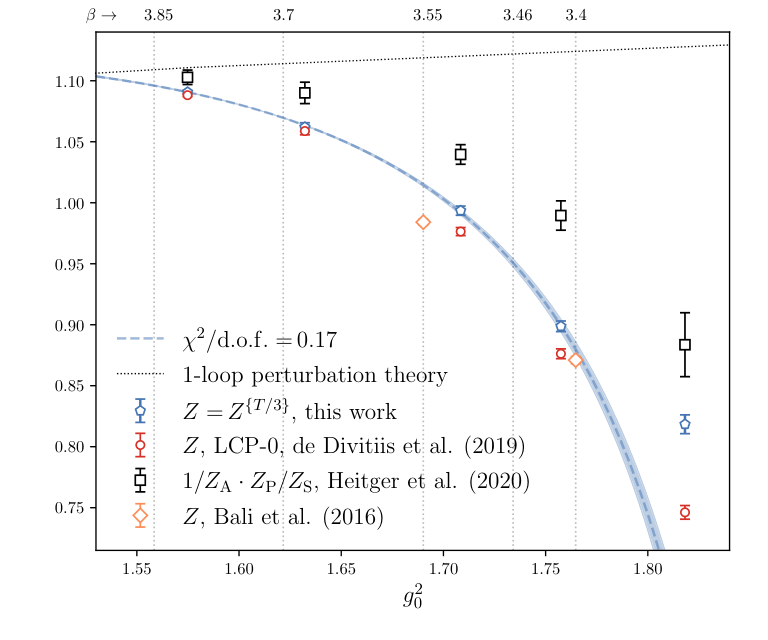
| this work | , LCP-0 de Divitiis et al. | , LCP-1 de Divitiis et al. | Heitger et al. | |
|---|---|---|---|---|
| 3.3 | 0.8184(77) | 0.7462(56) | 0.7896(36) | 0.884(26) |
| 3.414 | 0.8987(43) | 0.8762(40) | 0.8992(26) | 0.990(12) |
| 3.512 | 0.9935(38) | 0.9764(33) | 0.9861(23) | 1.0396(80) |
| 3.676 | 1.0621(36) | 1.0588(31) | 1.0611(23) | 1.0901(89) |
| 3.81 | 1.0907(13) | 1.0882(11) | 1.0884(8) | 1.1029(61) |
In order to confirm this claim of consistency (leaving aside higher cut-off effects) we construct ratios of different determinations and investigate their behaviour as a function of the lattice spacing. Interestingly, rather than , leading cut-off effects of can be identified in the ratio , as seen in Fig. 9 (left). The scaling behaviour of our results compared to those of previous works is shown in Fig. 9 (right). All ratios are fitted with an ansatz , excluding the coarsest lattice spacing. When adding a term linear in the lattice spacing, its fit parameter vanishes within its uncertainty in all cases. In conclusion, these scaling tests indicate that our results for are in accordance with the theoretical expectation of ambiguities or higher which by virtue of the imposed line of constant physics decrease monotically towards the continuum limit.
In addition, we interpolate our data using a Padé ansatz, constrained to the one-loop prediction of Ref. [52] for small couplings; see eq. (C.1) and Fig. 8. Owing to relevant higher order cut-off effects, shown in the right panel of Fig. 9, we do not include the coarsest lattice spacing in the fit. Other than that, it must be noted that the coarsest lattice spacing is well outside the range of CLS couplings. We obtain
| (C.1a) | |||
| where | |||
| (C.1b) | |||
| and | |||
| (C.1c) | |||
Our results at the CLS couplings are gathered in Table 7 and compared to those of Ref. [14] for two different LCP conditions. The two outmost CLS values ( and ) lie outside the range of our fitted estimates, so they are obtained by extrapolation. Their systematic errors are estimated from the statistical uncertainty of the nearest data point: the systematic error of is the statistical error of and that of is the statistical error of . These systematic errors are added to the statistical ones in quadrature.
| interpolated, this work | , LCP-0 de Divitiis et al. | , LCP-1 de Divitiis et al. | |||
|---|---|---|---|---|---|
| 3.4 | |||||
| 3.46 | |||||
| 3.55 | |||||
| 3.7 | |||||
| 3.85 |
References
- [1] M. Bochicchio, L. Maiani, G. Martinelli, G. C. Rossi and M. Testa, Chiral Symmetry on the Lattice with Wilson Fermions, Nucl. Phys. B 262 (1985) 331.
- [2] L. Maiani, G. Martinelli, M. L. Paciello and B. Taglienti, Scalar Densities and Baryon Mass Differences in Lattice QCD With Wilson Fermions, Nucl. Phys. B 293 (1987) 420.
- [3] G. Martinelli, C. Pittori, C. T. Sachrajda, M. Testa and A. Vladikas, A General method for nonperturbative renormalization of lattice operators, Nucl. Phys. B 445 (1995) 81, [hep-lat/9411010].
- [4] C. Sturm, Y. Aoki, N. H. Christ, T. Izubuchi, C. T. C. Sachrajda and A. Soni, Renormalization of quark bilinear operators in a momentum-subtraction scheme with a nonexceptional subtraction point, Phys. Rev. D 80 (2009) 014501, [0901.2599].
- [5] S. Capitani, M. Lüscher, R. Sommer and H. Wittig, Non-perturbative quark mass renormalization in quenched lattice QCD, Nucl. Phys. B 544 (1999) 669, [hep-lat/9810063]. [Erratum: Nucl. Phys. B 582, 762 (2000)].
- [6] M. Dalla Brida, S. Sint and P. Vilaseca, The chirally rotated Schrödinger functional: theoretical expectations and perturbative tests, JHEP 08 (2016) 102, [1603.00046].
- [7] G. M. de Divitiis and R. Petronzio, Nonperturbative renormalization constants on the lattice from flavor nonsinglet Ward identities, Phys. Lett. B 419 (1998) 311, [hep-lat/9710071].
- [8] T. Bhattacharya, S. Chandrasekharan, R. Gupta, W.-J. Lee and S. R. Sharpe, Nonperturbative renormalization constants using Ward identities, Phys. Lett. B 461 (1999) 79, [hep-lat/9904011].
- [9] T. Bhattacharya, R. Gupta, W.-J. Lee and S. R. Sharpe, Order a improved renormalization constants, Phys. Rev. D 63 (2001) 074505, [hep-lat/0009038].
- [10] M. Guagnelli, R. Petronzio, J. Rolf, S. Sint, R. Sommer and U. Wolff, Non-perturbative results for the coefficients and in improved lattice QCD, Nucl. Phys. B 595 (2001) 44, [hep-lat/0009021].
- [11] T. Bhattacharya, R. Gupta, W. Lee and S. R. Sharpe, Scaling behavior of discretization errors in renormalization and improvement constants, Phys. Rev. D 73 (2006) 114507, [hep-lat/0509160].
- [12] P. Fritzsch, J. Heitger and N. Tantalo, Non-perturbative improvement of quark mass renormalization in two-flavour lattice QCD, JHEP 08 (2010) 074, [1004.3978].
- [13] G. S. Bali, E. E. Scholz, J. Simeth and W. Söldner, Lattice simulations with improved Wilson fermions at a fixed strange quark mass, Phys. Rev. D 94 (2016) 074501, [1606.09039].
- [14] G. M. de Divitiis, P. Fritzsch, J. Heitger, C. C. Köster, S. Kuberski and A. Vladikas, Non-perturbative determination of improvement coefficients and and normalisation factor with Wilson fermions, Eur. Phys. J. C 79 (2019) 797, [1906.03445].
- [15] J. Heitger, F. Joswig and A. Vladikas, Ward identity determination of for lattice QCD in a Schrödinger functional setup, Eur. Phys. J. C 80 (2020) 765, [2005.01352].
- [16] G. Bali, S. Bürger, S. Collins, M. Göckeler, M. Gruber, S. Piemonte et al., Nonperturbative Renormalization in Lattice QCD with three Flavors of Clover Fermions: Using Periodic and Open Boundary Conditions, 2012.06284.
- [17] T. Bhattacharya, R. Gupta, W. Lee, S. R. Sharpe and J. M. Wu, Improved bilinears in lattice QCD with non-degenerate quarks, Phys. Rev. D 73 (2006) 034504, [hep-lat/0511014].
- [18] M. Constantinou, M. Hadjiantonis, H. Panagopoulos and G. Spanoudes, Singlet versus nonsinglet perturbative renormalization of fermion bilinears, Phys. Rev. D 94 (2016) 114513, [1610.06744].
- [19] M. Lüscher and P. Weisz, On-Shell Improved Lattice Gauge Theories, Commun. Math. Phys. 97 (1985) 59. [Erratum: Commun. Math. Phys. 98, 433 (1985)].
- [20] B. Sheikholeslami and R. Wohlert, Improved Continuum Limit Lattice Action for QCD with Wilson Fermions, Nucl. Phys. B 259 (1985) 572.
- [21] M. Bruno et al., Simulation of QCD with flavors of non-perturbatively improved Wilson fermions, JHEP 02 (2015) 043, [1411.3982].
- [22] M. Bruno, T. Korzec and S. Schaefer, Setting the scale for the CLS flavor ensembles, Phys. Rev. D 95 (2017) 074504, [1608.08900].
- [23] D. Mohler, S. Schaefer and J. Simeth, CLS flavor simulations at physical light- and strange-quark masses, EPJ Web Conf. 175 (2018) 02010, [1712.04884].
- [24] J. Heitger, F. Joswig, A. Vladikas and C. Wittemeier, Non-perturbative determination of and in lattice QCD, EPJ Web Conf. 175 (2018) 10004, [1711.03924].
- [25] J. Heitger and F. Joswig, The renormalised improved vector current in three-flavour lattice QCD with Wilson quarks, Eur. Phys. J. C 81 (2021) 254, [2010.09539].
- [26] J. Bulava, M. Della Morte, J. Heitger and C. Wittemeier, Nonperturbative renormalization of the axial current in lattice QCD with Wilson fermions and a tree-level improved gauge action, Phys. Rev. D 93 (2016) 114513, [1604.05827].
- [27] J. Bulava, M. Della Morte, J. Heitger and C. Wittemeier, Non-perturbative improvement of the axial current in lattice QCD with Wilson fermions and tree-level improved gauge action, Nucl. Phys. B 896 (2015) 555, [1502.04999].
- [28] L. Chimirri, P. Fritzsch, J. Heitger, F. Joswig, M. Panero, C. Pena et al., Non-perturbative renormalization of improved tensor currents, PoS LATTICE2019 (2020) 212, [1910.06759].
- [29] M. Bruno, I. Campos, P. Fritzsch, J. Koponen, C. Pena, D. Preti et al., Light quark masses in lattice QCD with Wilson fermions, Eur. Phys. J. C 80 (2020) 169, [1911.08025].
- [30] J. Heitger, F. Joswig and S. Kuberski, Determination of the charm quark mass in lattice QCD with flavours on fine lattices, 2101.02694.
- [31] G. S. Bali et al., The strange and light quark contributions to the nucleon mass from Lattice QCD, Phys. Rev. D 85 (2012) 054502, [1111.1600].
- [32] G. S. Bali, S. Collins, D. Richtmann, A. Schäfer, W. Söldner and A. Sternbeck, Direct determinations of the nucleon and pion terms at nearly physical quark masses, Phys. Rev. D 93 (2016) 094504, [1603.00827].
- [33] S. Aoki et al., FLAG Review 2019: Flavour Lattice Averaging Group (FLAG), Eur. Phys. J. C 80 (2020) 113, [1902.08191].
- [34] K. Ottnad, Excited states in nucleon structure calculations, in 38th International Symposium on Lattice Field Theory, 11, 2020. 2011.12471.
- [35] J. Green, Systematics in nucleon matrix element calculations, PoS LATTICE2018 (2018) 016, [1812.10574].
- [36] M. Lüscher, S. Sint, R. Sommer and P. Weisz, Chiral symmetry and improvement in lattice QCD, Nucl. Phys. B 478 (1996) 365, [hep-lat/9605038].
- [37] J. Bulava and S. Schaefer, Improvement of lattice QCD with Wilson fermions and tree-level improved gauge action, Nucl. Phys. B 874 (2013) 188, [1304.7093].
- [38] M. Lüscher and S. Schaefer. http://luscher.web.cern.ch/luscher/openQCD.
- [39] A. D. Kennedy, I. Horvath and S. Sint, A New exact method for dynamical fermion computations with nonlocal actions, Nucl. Phys. Proc. Suppl. 73 (1999) 834, [hep-lat/9809092].
- [40] M. A. Clark and A. D. Kennedy, Accelerating dynamical fermion computations using the rational hybrid Monte Carlo (RHMC) algorithm with multiple pseudofermion fields, Phys. Rev. Lett. 98 (2007) 051601, [hep-lat/0608015].
- [41] M. Lüscher, S. Sint, R. Sommer, P. Weisz and U. Wolff, Non-perturbative O(a) improvement of lattice QCD, Nucl. Phys. B 491 (1997) 323, [hep-lat/9609035].
- [42] P. Perez-Rubio, S. Sint and S. Takeda, An O(a) modified lattice set-up of the Schrödinger functional in SU(3) gauge theory, JHEP 07 (2011) 116, [1105.0110].
- [43] L. Del Debbio, H. Panagopoulos and E. Vicari, dependence of SU(N) gauge theories, JHEP 08 (2002) 044, [hep-th/0204125].
- [44] P. Fritzsch, A. Ramos and F. Stollenwerk, Critical slowing down and the gradient flow coupling in the Schrödinger functional, PoS Lattice2013 (2014) 461, [1311.7304].
- [45] U. Wolff, Monte Carlo errors with less errors, Comput. Phys. Commun. 156 (2004) 143, [hep-lat/0306017]. [Erratum: Comput. Phys. Commun. 176, 383 (2007)].
- [46] S. Schaefer, R. Sommer and F. Virotta, Critical slowing down and error analysis in lattice QCD simulations, Nucl. Phys. B 845 (2011) 93, [1009.5228].
- [47] A. Ramos, Automatic differentiation for error analysis of Monte Carlo data, Comput. Phys. Commun. 238 (2019) 19, [1809.01289].
- [48] P. T. Boggs and J. E. Rogers, Orthogonal distance regression, tech. rep., National Institute of Standards and Technology, Gaithersburg, MD, 1989. 10.6028/NIST.IR.89-4197.
- [49] M. Dalla Brida, T. Korzec, S. Sint and P. Vilaseca, High precision renormalization of the flavour non-singlet Noether currents in lattice QCD with Wilson quarks, Eur. Phys. J. C 79 (2019) 23, [1808.09236].
- [50] A. Gerardin, T. Harris and H. B. Meyer, Nonperturbative renormalization and -improvement of the nonsinglet vector current with Wilson fermions and tree-level Symanzik improved gauge action, Phys. Rev. D 99 (2019) 014519, [1811.08209].
- [51] S. Sint and P. Weisz, Further results on O(a) improved lattice QCD to one loop order of perturbation theory, Nucl. Phys. B 502 (1997) 251, [hep-lat/9704001].
- [52] S. Aoki, K.-i. Nagai, Y. Taniguchi and A. Ukawa, Perturbative renormalization factors of bilinear quark operators for improved gluon and quark actions in lattice QCD, Phys. Rev. D 58 (1998) 074505, [hep-lat/9802034].