Randomness of Möbius coefficents and Brownian Motion:
Growth of the Mertens Function and the Riemann Hypothesis
Abstract
The validity of the Riemann Hypothesis (RH) on the location of the non-trivial zeros of the Riemann -function is directly related to the growth of the Mertens function , where is the Möbius coefficient of the integer : the RH is indeed true if the Mertens function goes asymptotically as , where is an arbitrary strictly positive quantity. We argue that this behavior can be established on the basis of a new probabilistic approach based on the global properties of Mertens function, namely, based on reorganizing globally in distinct blocks the terms of its series. To this aim, we focus the attention on the square-free numbers and we derive a series of probabilistic results concerning the prime number distribution along the series of square-free numbers, the average number of prime divisors, the Erdős-Kac theorem for square-free numbers, etc. These results point to the conclusion that the Mertens function is subject to a normal distribution as much as any other random walk. We also present an argument in favor of the thesis that the validity of the Riemann Hypothesis also implies the validity of the Generalized Riemann Hypothesis for the Dirichlet -functions. Next we study the local properties of the Mertens function, i.e. its variation induced by each Möbius coefficient restricted to the square-free numbers. Motivated by the natural curiosity to see how close to a purely random walk is any sub-sequence extracted by the sequence of the Möbius coefficients for the square-free numbers, we perform a massive statistical analysis on these coefficients, applying to them a series of randomness tests of increasing precision and complexity: together with several frequency tests within a block, the list of our tests include those for the longest run of ones in a block, the binary matrix rank test, the Discrete Fourier Transform test, the non-overlapping template matching test, the entropy test, the cumulative sum test, the random excursion tests, etc. for a total number of eighteen different tests. The successful outputs of all these tests (each of them with a level of confidence of that all the sub-sequences analyzed are indeed random) can be seen as impressive “experimental” confirmations of the brownian nature of the restricted Möbius coefficients and the probabilistic normal law distribution of the Mertens function analytically established earlier. In view of the theoretical probabilistic argument and the large battery of statistical tests, we can conclude that while a violation of the RH is strictly speaking not impossible, it is however extremely improbable.
.
.
I Introduction
In Physics there are innumerable examples of a successful scientific strategy which consists of the following steps:
-
A Start from a consolidated set of empirical data.
-
B Elaborate a theory which explains the data: besides its elegance and beauty, the strength of the proposed theory is related to the diversity of phenomena it can explain, together with its simplicity and parsimony.
-
C Make repeated testable and thorough attempts to falsify the theory. When theories are falsified by such observations, scientists can respond by revising the theory, or by rejecting the theory in favor of another one. In either case, however, this process must aim at the production of new, falsifiable predictions.
Elaborating a theory is of course something different than proving a theorem, even though a theory may be based on theorems or may give rise to several theorems: , i.e. Newton’s law, expresses a theory of mechanics rather than a theorem that nobody can prove it. However, it is true that, assuming the validity of Newton’s theory, there are of course several theorems which follow from it, e.g. the conservation of energy for conservative forces. The success of Newton’s theory is certified, for instance, by showing the validity to Kepler’s laws while its limit turns out to be the existence of relativistic phenomena. Another striking example of this successful strategy in Physics comes from atomic phenomena: based on a huge and consolidate set of spectroscopic data, Heisenberg, Schrödinger and many others set up and developed the theory of Quantum Mechanics. While it does not make any sense to ask whether one can prove the Schrödinger equation, it is on the contrary extremely crucial to check that all its consequences are not only theoretically self-consistent but also never contradicted by any experiment.
These considerations are particularly useful in order to put in the right perspective the approach we are going to present for facing an interesting scientific problem which does not come however from the realm of physical phenomena but, on the contrary, directly from the realm of mathematics. It concerns an infinite class of functions of the complex variable , the so-called Dirichlet -functions, to which belongs Riemann’s zeta function. Postponing to later chapters the discussion of all relevant details, a guideline for the present paper can be summarized as follows:
- 1.
For the problem at hand, the consolidate set of empirical data of the problem consists of the explicit computation of a huge number of the so-called non-trivial zeros of these functions in the complex plane of the variable . As a matter of fact, all these computed zeros are found to be always on the line . So far there are no theorems which make such a property of these functions obvious and this is precisely why the problem is interesting and challenging for a curious mind. The possibility that all the non-trivial zeros of the Dirichlet -functions are indeed on the line is known in the literature as the Generalized Riemann Hypothesis (GRH).
- 2.
As shown in the following, we are able to argue that there exists a very simple and elegant theory which explains at once why all non-trivial zeros of all the Dirichlet -functions are always on the line : according to this theory, any Dirichlet -function is associated to a particular realization of a Brownian motion which – it can be shown – rules the location of its zeros. The ubiquitous value for the real part of all the zeros of these functions finds then a natural explanation in terms of the universal critical exponent associated to the growth of any Brownian motion and the validity of a central limit theorem behind any Dirichlet -function.
- 3.
Since what is proposed in this paper is an overall theory for the zeros of the Dirichlet functions rather than a theorem, in the last part of the paper we have performed a large number of testable attempts to falsify it. These consist of a huge battery of “numerical experiments” designed to bring under a severe scrutiny the many different aspects of the supposed Brownian motion behind the Dirichlet -functions. As discussed in detail later, the successful outputs (with an extremely high level of confidence, as certified by standard statistical tests) of all the numerical analyses performed can be seen as impressive experimental confirmation of the theoretical framework proposed for the GRH. In this respect, we invite the reader to simply look at the various figures presented in the last part of the paper, showing spectacular agreement between the Brownian motion theory and the numerics.
As will become more and more clear in the following pages, in order to set up and support the Brownian motion picture behind the Dirichlet -functions we had to embark in a long and detailed tour of many fascinating fields in physics and mathematics coming, in particular, from the common area of probability, stochastic phenomena and alike. The ideas which guide our work will be often illustrated with elementary arguments which have the clear advantage to present, in an essential way, the results we obtained: it is worth stressing that the style adopted in the presentation is the one of a theoretical physicist rather than a mathematician. In this respect, we do not claim to have any rigorous proof of the results presented here but we like to think that our work has been guided by the famous and beautiful Feynman’s comment: A great deal more is known than has been proved. Moreover, if this work will have the effect to stimulate further rigorous studies by genuine mathematicians on the subject, it has already reached the scope to draw the attention to a possible way to tackle a long standing problem such as Riemann’s hypothesis.
To make crystal clear the style adopted in this paper, let’s present a paradigmatic and important example of a result which will be extremely useful later. Such an example concerns the square-free numbers. An integer is said to be square free if no prime factor divides it more than once and these square free numbers will play an important role in the sequel of the paper. Let us pose the following question: What is the probability that an integer is square-free? This is equivalent to asking: What is the density of square-free numbers among the integers? To answer this question, our way of arguing will go as follows11 1 This argument is presented in the book by M. Schröder Schroeder listed in our references, a text which is a true gem in the relations between Number Theory and Physics.: assuming the statistical independence of primes, the probability that a number is not divisible twice by the same prime is approximatively and, multiplying on all the primes, we get
| (1) |
Obviously, the first part of the line above plays the role of a theory, while the second part is a mathematical identity, i.e. a theorem. But, can we check the validity of this theory? Yes, by simply counting the fraction of square free numbers within the integers! Doing this numerical experiment, with the corresponding plot shown in Figure 1, one can see that, quite rapidly, the measured density of square-free numbers within the integers indeed tends to the predicted theoretical value .
This example follows paradigmatically the A-B-C scheme mentioned above, since it elaborates a theory based on some assumption, it leads to a theorem (the infinite product on primes given above is indeed equal to ) and it is not falsified by a direct experiment. Of course the argument misses any mathematical rigor since, for instance, it never specifies how the probability is defined, if there is a proof of the independence of the divisibility of an integer by two prime numbers and , what is the actual meaning of the symbol , and finally the value to assign to a “numerical check” of a mathematical property. We appeal once more to Feynman to go on with our presentation.
A final disclaimer: this paper is rather long, however, by no means should it be regarded as a review of the (Generalised) Riemann Hypothesis and the associated literature: the reader interested in the history of the GRH may find satisfaction in reading some of the large literature specialized to this subject such as, for instance Riemann, Edwards, Titcmarsh, Davenport, Bombieri, Sarnak, Conrey, Polya, Borwein, Broughan, reviewRiemann, Wolf.
Let’s now go to the next section which provides a general overview of the topic and a presentation of the various parts of the paper.
II A bird’s eye view of the problem
An interesting aspect of the studies presented in this paper is the connection with the “experimental” sides of mathematics, in particular those concerning with time series and the pseudorandom nature of their coefficients. Let’s explain briefly what this is about. Among other things, this paper deals indeed with an infinite binary sequence made up of ’s which looks like
| (2) |
It is assumed that we can have access to arbitrarily large parts of this sequence, although always finite. One of our purposes will be to establish whether is a random sequence and whether its properties are captured by the normal law distribution. As we will see, a relevant prior information on our sequence , which will be quite important in our analysis, is that such a sequence has on average an equal number of ’s and ’s. There is also additional information on the sequence which will be presented later and which help us in better pinpointing the pattern of the appearance of the ’s and ’s. We will discuss below the origin of this problem, as well as its deep connection with an old-standing question of Number Theory: the Riemann Hypothesis Riemann, Edwards, Titcmarsh, Davenport, Bombieri, Sarnak, Conrey, Polya, Borwein, Broughan, Apostol, Iwaniec, Bombieri2, Steuding, Sarnak2, BK0, BK00, BK000, BK1, BK2, BK3, BK4, Bost, Connes, KeatingSnaith, Sierra1, Sierra, Sierra2, Srednicki, Bender, reviewRiemann, Wolf, GriffinZagier, RodgersTao. It is however important to discuss some interesting methodological issues in these numerical studies.
II.1 Time series
If one does not have any prior information on an infinite sequence of numbers, the problem of establishing its nature can only be addressed statistically, i.e. in terms of a statistical study which generically goes under the name of Time Series Analysis, a well established and very powerful branch of Probability Theory Knuth, Nist, Marsaglia, Feller, Jaynes, timeseries1, timeseries2, timeseries3. It is worth stressing the power of this approach: using the Time Series Analysis to study sequences of numbers such as , one can reach very robust and significant conclusions on whether the sequence under scrutiny is random or not. Indeed, there is no limit to the number of tests that can be developed and applied to an infinite sequence of numbers like the ones in (2) to check its level of randomness. Some of these tests are rather simple while others, as we will see, can instead be very elaborate and sophisticated.
In pursuing this kind of analysis, of course there is always a lurking regressus ad infinitum objection to face: namely, if a sequence appears to be random under the tests , how can we be sure that it will also appear to be random under a new test ? We cannot, of course. Assume, however, that no matter how we increase the number and the quality of the statistical tests, any arbitrarily large parts of always passes them successfully. Well, at this point, our level of confidence of its randomness starts then to increase considerably, and we can quantify it in terms of a probability that becomes closer and closer to 1 as we increase the number and the refinement of our tests. In Donald Knuth’s words, “the sequence is presumed innocent until proven guilty” Knuth and it is more and more innocent by increasing the level of our screenings. One may even push such an argument forward and argue that this assumption is at the root of our general way of getting knowledge: to form a judgment about the likely truth or falsity of any proposition A, the correct procedure is to calculate the probability that A is true, conditional on all the evidences at hand Jaynes. In Physics these statements are, of course, very familiar: for instance, the discovery of the Higgs boson Higgs, where the ATLAS and CMS experiments at CERN’s Large Hadron Collider announced they had each observed a new particle in the mass region around 125 GeV, is after all a nice example of knowledge acquired by “statistics”, given that this new particle owes its existence only to the satisfaction of stringent statistical analysis of the events collected at LHC. In Mathematics, on the other hand, knowledge reached by probabilist arguments seems to be almost flawed by an inherent uncertainty. But is it always the case? To make some progress on this question, let’s discuss now in more detail the origin of our sequence.
II.2 Probability in Number Theory
Our sequence has an interesting origin and is deeply connected to one of the most famous problems in Number Theory, i.e. the Riemann conjecture about the location of the zeros of the Riemann zeta-function in the complex plane of the variable Riemann, Edwards, Titcmarsh, Davenport, Bombieri, Sarnak, Conrey, Polya, Borwein, Broughan, Apostol, Iwaniec, Bombieri2, Steuding, Sarnak2, BK0, BK00, BK000, BK1, BK2, BK3, BK4, Bost, Connes, KeatingSnaith, Sierra1, Sierra, Sierra2, Srednicki, Bender, reviewRiemann, Wolf, GriffinZagier, RodgersTao. As we will see, the problem is also related to a famous topic of Statistical Physics, i.e. the random walk problem Yuval, Mazo, Rudnick, Levy, diffusion and, in particular, how it is possible to establish the random nature of a Brownian motion when one has access to only one single trajectory rather then a collection of trajectories Perrin, Nordlund, Kappler, brow1, brow2, brow3, brow4. Although it is not surprising that probability concepts are applied to the study of Brownian motion, one may wonder what probability has to do instead with Number Theory, a world dominated by the rigid rules of integer numbers and the like. However, some of the most remarkable progress of the latest decades is that many properties of Number Theory can be strikingly captured by ideas, methods and results which come indeed from the realm of probability, that branch of mathematics which describes aleatoric events Schroeder, Kac, erdosbook, ErdosKac, Kubilius, Tao, Cramer, Billingsley, Dyson, Montgomery, Odlyzko, Rudnick-Sarnack, Grosswald, EPFchi, Franca1, ML, LM, Denjoy, Churchhouse. Among the pioneers of this probabilistic approach to Number Theory are Mark Kac Kac and Paul Erdős erdosbook. A nice example of what can be achieved by adopting such a point of view is provided by their famous Erdős-Kac theorem ErdosKac which states that, if we denote by the number of distinct prime factors of the integer , then in the large limit, the probability distribution of the variable
| (3) |
is the standard normal distribution , with mean and variance , where stands for the normal distribution of a random variable with mean and variance given by
| (4) |
It is important to emphasize that regardless of the fact that is a completely deterministic arithmetic function, the distribution of its values follow the probabilistic normal distribution. Both the normal distribution and the Erdős-Kac theorem will accompany us in the course of our discussion and we will have the opportunity to comment more on their importance. Here, the “randomness” is related to the fact that the event of an integer being divisible by a prime is independent of being divisible by another prime . This is in essence the origin of randomness in this paper.
II.3 Riemann-zeta function
Referring all the details to the coming Sections, let’s see the context in which our sequence (2) emerges. Consider the Riemann zeta function , given by its series and infinite product representation on the prime numbers (), hereafter ordered wrt their increasing values
| (5) |
The above definition converges for , and the function can be analytically continued to the whole complex plane. This function has a pole at , an infinite number of (trivial) zeros at (where and an infinite number of other zeros in the critical strip which are supposed to satisfy the Riemann Hypothesis Riemann, Edwards, Titcmarsh, Davenport, Bombieri, Sarnak, Conrey, Polya, Borwein, Broughan, Apostol, Iwaniec, Bombieri2, Steuding, Sarnak2, BK0, BK00, BK000, BK1, BK2, BK3, BK4, Bost, Connes, KeatingSnaith, Sierra1, Sierra, Sierra2, Srednicki, Bender, reviewRiemann, Wolf, GriffinZagier, RodgersTao:
Riemann Hypothesis (RH): in the critical strip , the zeros of are all and only on the infinite line .
Equivalently, if the RH is true, the multiplicative inverse function of , defined as well as by its series and infinite product representation
| (6) |
must necessarily have all its poles along the line . The arithmetic function , known as the Möbius function, has values
| (7) |
Using the Stieltjes measure, we can express in terms of its inverse Mellin transform
| (8) |
where is the so-called Mertens function, given by
| (9) |
It is then simple to see that, if asymptotically goes as , for any arbitrarily small positive , then the RH is indeed true: in this case, in fact, the integral (8) diverges at , making clear the presence of a singularity on this axis 22 2 Throughout this paper, the symbol signifies the “big O” notaton, for any arbitrarily small and positive . We will not always indicate the and may write simply .. In the following we will call this approach to the RH the statistical/horizontal approach, to be compared later with the quantum/vertical approaches to the RH.
II.4 Law of iterated log’s
Note that all terms with do not contribute to the sum in and that the non-zero values of only come from square-free numbers. As we have seen in eq.(1), these numbers are a finite fraction of all integers. Their first representatives are
| (10) |
and the -th square-free number scales as
| (11) |
Let’s then introduce the map such that and, restricting the attention only to these square-free numbers, let’s also define
| (12) |
The relation of these coefficients with our initial is simply
| (13) |
In the following we will also denote these coefficients as . For our future considerations, in particular those concerning with the statistical analysis, sometimes we find it useful to deal with our original sequence while in other cases we find it more useful to focus our attention on the sequence , keeping in mind that the relationship between the two quantities is expressed by eq. (13). It is important to stress that, focusing the attention only on the values taken by the Möbius coefficients on square-free numbers is the way to avoid all ‘‘periodicities”33 3 We have, for instance, that whenever is multiple of , , , , etc., and, in general, a multiple of any or . These considerations imply that has many multiplicative periodicities while is expected to have none. present in the original arithmetic function and, therefore, to better evaluate the random properties of this function which emerge by considering its restriction to the square-free numbers. In other words, we take seriously the observation on made originally by Denjoy Denjoy (see also the book by Edwards Edwards p. 268) and we develop the main heuristic of this paper based precisely on the pseudo-random properties of the restricted Möbius coefficients to the square-free numbers.
In the following the final object of our study is the restricted Mertens function , i.e. the Mertens function restricted to the square-free numbers only
| (14) |
Notice that, in light of the scaling law (11), we have the scaling relation
| (15) |
If we could show that the sequence follows the stochastic laws of a random motion, then for the asymptotic growth of we would have
| (16) |
for an arbitrarily small positive , which, as explained above, leads to an understanding of the origin and the validity of the RH.
To show that has indeed such a behaviour, in the Part B of this paper we will present a global approach44 4 As it will become clear in Sections XII and XIII, the terminology global approach refers to the possibility of studying the function by grouping globally and at once large sets of its coefficients . In contrast, we will refer to the local property of the function when we focus our attention just on the individual coefficients . to this function which involves the prime number distribution along the series of square-free numbers, the average number of prime divisors, the Erdős-Kac theorem for square-free numbers, etc. Moreover, we will rely on the law of iterated logarithm which describes the magnitude of the fluctuations of a random walk Feller to argue that, asymptotically, for the fluctuations of the function we have55 5 For the original Mertens function such a behavior (with different coefficient) was also conjectured in Churchhouse on the basis of some computer studies: the analysis pursued here not only significantly enlarges the set of theoretical tools which leads to understand the validity of the formula (17) but also provides for the first time a very robust support to the random behavior of any sufficiently large subsequence of on the basis of many and very sophisticated statistical tests.
| (17) |
where “a.s.” stands for “almost surely”, in a probabilistic sense, i.e. with probability equal to Feller. As is well known, this law of iterated logarithm applies to all Brownian motion random sequences
| (18) |
where are random uncorrelated variables. The quantity is plotted in Figure 2.a for and compared in Figure 2.b with the behavior of an analogous quantity computed for several random uncorrelated sequences. These figures are purely illustrative of the brownian motion behavior of the restricted Mertens sequence which, as we will explicitly check in great detail later, persists to all scales, i.e. no matter how much we enlarge the interval in which we study this sequence.
It is worth stressing that there is nothing which prevents a deterministic sequence from being a realization of a random process, and the restricted Möbius coefficients together with the associate Mertens function seem indeed to be a very good example of this fact. For instance, imagine the random process of a person flipping a coin a large number of times, and recording the sequence of the outcome of the flips as a list in a sacred book kept in a secure chamber in a church, or the National Bureau of Standards. The existence of the book now makes the sequence completely deterministic, since anyone can access the book, and everyone agrees on its precise content. It’s a rather boring book and, unlike the gambler, an individual feels no nervous anticipation of what will be the next flip, since it is already all known to anyone.


II.5 Generalized Riemann Hypothesis
To put the problem in a proper perspective, it is very useful to remind (see Part A for further details) that the Riemann -function is just a particular case of a more general class of analytic functions known as Dirichlet L-functions , where is an arithmetic character which we will discuss in more detail in Section III of Part A. There are infinitely many of these functions in relation to the infinitely many characters and, for , they admit both an infinite series and product representation
| (19) |
For all these functions, the Generalized Riemann-Hypothesis has been conjectured to hold:
Generalized Riemann Hypothesis (GRH): in the critical strip , the zeros of all the infinitely many L-functions are all and only on the infinite line .
Notice that
| (20) |
and this function can be expressed in terms of its inverse Mellin transform
| (21) |
where the analog of the Mertens function for the Riemann zeta function is played in this case by
| (22) |
which we call the Generalized Mertens function. As in the case of the Riemann zeta function, if it can be shown that goes asymptotically as , for any arbitrarily small , then the GRH is indeed true. We will discuss later the relation which links together to (see Section VIII) and, in view of this relation, how it is possible to unify the two hypothesis, in particular, how it is possible to argue that the validity of the GRH can be considered as a consequence of the RH.
Let us stress that one of the key features of the statistical approach to the RH pursued in this paper is its level of naturalness and universality which helps in clarifying at once why all the infinite number of Dirichlet -functions (including the Riemann -function) have all their non-trivial zeros on the line66 6 Denoting by the position of a generic zero of a Dirichlet function, it is worth to point out that the statistical approach presented here is extremely powerful in identifying the abscissa of all these zeros, leading to the conclusion that for all of them , but it is literally unable to address the positions of their imaginary part . On the other hand, one should keep in mind that the imaginary parts of these zeros are not at all universal since they change by changing the -functions. . As it will become clear later, the reason is indeed quite interesting: the location of all the zeros of all these functions are ruled by sequences of numbers which, albeit strictly deterministic, behave though as brownian random walks! In other words, the universal location on the line of all the zeros of these functions can be traced back to the universal statistical properties of the brownian random walks, such as the existence of the central limit theorem or the validity of the law of iterated log’s.
II.6 Organization of the paper
The paper is divided into four Parts, each of them addresses different aspects of the problem and therefore has a different style and length.
Part A presents the general framework of the Dirichlet -functions and explains why we can consider the Riemann zeta-function as a particular example thereof. We discuss in particular the reason why the argument which we previously used to show the validity of the GRH for the -functions of non-principal characters ML, LM cannot be used to show the RH for the Riemann zeta-function. However, we argue that the validity of the RH would imply the validity of the GRH. In Part A we also discuss some important results about the properties of the Dirichlet -functions which justify the use of a probabilistic approach for the GRH. We recall, in particular, both the theorem by Grosswald and Schnitzer Grosswald concerning a set of random functions which share the same zeros of the Dirichlet (Riemann) functions in the critical strip, and our previous results on the location of the zeros of the Dirichlet L-functions of non-principal characters. So, besides the original section on the relation between the RH and the GRH, Part A contains well known but also less known properties of the Dirichlet functions and is meant to be just a reference part for the rest of the paper, where the reader can easily find the most relevant definitions, the discussion of some key features of these functions, as well as some key points of our approach.
Part B is the core original theoretical part of this paper, where we present our new approach to the restricted Mertens function, which we call the global approach. It concerns a series of new results relative to the sequence of the square-free numbers which lead us to argue positively about the validity of the RH on the basis of a probabilistic argument. In this part of the paper, we address important issues of Number Theory such as the distribution of prime numbers along the sequence of the square free-numbers, the important role of the primorial (the equivalent of the factorial for the prime numbers) in controlling the growth of the Mertens functions, the average number of prime divisors, the Poissonian distribution satisfied by the prime divisors and the Erdős-Kac theorem for square-free numbers. All these results are instrumental for us to argue that the moments of the restricted Mertens function asymptotically behave as those of a random walk, i.e.
| (23) |
The careful reader may have noticed that the expressions above refer to some average quantities, i.e. . We will explain the meaning of taking such an average for a deterministic sequence as the one given by the Möbius coefficients, and this leads us, in particular, to define the proper statistical ensemble in which this average makes sense. As we will see, the problem is remarkably close to the so-called Single Trajectory Random Walk problem Nordlund, Kappler, brow1, brow2, brow3, brow4, which consists in establishing the random nature of a brownian motion when one has access to only one single trajectory rather then a collection of trajectories. In a nutshell, we will see that all the considerations related to the average of the restricted Mertens function have a precise analog in statistical mechanics, when one substitutes phase space average with time average, under the assumption of the ergodicity and time translation of the system under scrutiny.
Part C presents a large battery of statistical tests which we have performed on very long sub-sequences of the restricted Möbius coefficients. Altogether 18 statistical tests were performed, each of them repeated thousands of times in very large intervals along the infinite sequence of the restricted Möbius coefficients . All these studies aim to probe the local properties of and the associated restricted Mertens function and they were triggered by our natural curiosity to see how good such finite sub-sequences behave randomly, as predicted on the basis of the global theoretical considerations on the restricted Mertens function that we presented in Part B. In this part we extensively use the block variables associated to the sub-sequences of ’s for reaching very robust probabilistic conclusions on a deterministic sequence as the one given by the restricted Martens sequences . The statistical tests applied to our sequence are of increasing order of complexity and sophistication. Let’s anticipate and, at the same time emphasize, that all the sub-sequences analyzed passed successfully our statistical tests, with an overall level of confidence of , as quantified by the associated distribution. To the best of our knowledge, never before has such a massive statistical analysis been performed on the restricted Möbius coefficients and Mertens function, and the outputs of this analysis may be regarded as a very robust and striking “experimental” confirm of the RH. .
Part D contains our conclusions. In this section we come back to the relationship between GRH and RH and we also make a comparison of our result versus other conjectured results concerning the growth of the Mertens function. We will comment, in particular, on some unpublished conjectured formulas due to Gonek which were obtained, though, assuming the validity of the RH. We will show that our prediction on the growth of the restricted Mertens function, obtained without assuming the validity of the RH77 7 As a matter of fact, our logic has been the reverse! Namely, the Riemann Hypothesis holds true on the basis of the behavior we have established for the restricted Mertens function., is perfectly compatible with the estimated growth of the restricted Mertens function obtained assuming the Riemann Hypothesis.
Notation. In the following we often use the index to refer to the square-free numbers and quantities related to them. For an arithmetic function defined over the integers, the same function over the square free numbers will be denoted as . This applies to the restricted Mertens function given in eq. (14), the restricted Möbius function, prime number counting function and number of divisors functions , and defined below. On the other hand, we use and to label a generic integer and to denote a generic real number, whose integer part are related to the integers. It is of course simpler to use rather than for denoting intervals but one has to keep in mind that is the true number of terms in a sum as the one in (14). The scaling relation between and is given in eq. (11) and illustrated in Figure 3. Moreover, as usual, in the following we use the notation
| (24) |
to denote the real and imaginary parts of the complex variable .
PART A
The aim of this part is to clarify a few important points of the subject that help in illuminating the nature of the RH. As we are going to see, a crucial role in our future discussions is played by probabilistic arguments, characterised by their economy and simplicity. Moreover, they provide a natural way to provide a concrete reason for the validity of the Riemann and the Generalized Riemann Hypothesis. Indeed, the probabilistic approach pursued in this paper has the advantage to disclose, in a very natural way, the reason why the non-trivial zeros of the Riemann zeta-function have to be along the line in the complex plane and, at the same time, why this property is also shared by the infinitely many Dirichlet -functions. In other words, if arguments based on probability provide on one side a very robust ground of naturalness for the Riemann and the Generalised Riemann Hypothesis, on the other side they also point to the very high level of universality behind these hypotheses, ultimately related to the properties of the random walk, i.e. to the ubiquitous appearance of the normal law distribution and the central limit theorem.
In this part of the paper we show that the Riemann zeta functions belongs to an infinitely large class of functions known as Dirichlet -functions: these may be regarded as generating functions constructed in terms of local data associated with an arithmetic object. Dirichlet -functions are particular examples of so-called Dirichlet series, which provide very useful tools in analytic number theory. One of the main properties of the Dirichlet series is their half-plane absolute convergence. In the case of the -functions, another important property is that, besides their series representation, they also admit an infinite product representation over prime numbers. In the following, we will give a very short overview of the -functions, in particular focusing on their origin from number theory and their analytic structure in the complex plane, referring to classical texts of the literature for an extended discussion of their properties Apostol, Iwaniec, Bombieri2, Steuding, Sarnak2.
Setting the stage. The main purpose of this Part is to set the stage for the results presented later in this paper. In the next sections, in particular, we intend to clarify the following topics:
- •
Why is the Riemann zeta function a particular example of the Dirichlet -functions?
- •
- •
Would it be possible to show that the validity of RH implies the validity of the GRH?
- •
What is the importance of the Grosswald-Schnitzer theorem on the zeros of a set of random functions which are the analogue of the Dirichlet -functions?
- •
What is the difference between the Statistical Approach and the Quantum Approach for establishing the validity of the Generalized Riemann Hypothesis?
- •
What do we know so far about the properties of the Mertens function and where does this knowledge come from?
Playing with dice. As we will see shortly, the answer to the first two questions is very straightforward: any Dirichlet -function is associated to a natural number , known as the modulus, and the Riemann zeta-function simply corresponds to the case. Moreover, we will show that, behind all these functions, there is a stochastic process which may be regarded as the outputs of a dice made of faces. Hence, for the Riemann zeta-function, we are formally dealing with a dice having only face, which is what makes it difficult to apply our previous approach ML, LM directly to . A signature of this issue is the pole at for Dirichlet L-functions based on principal characters, which is absent for those based on non-principal characters. As a matter of fact, this difficulty is what motivated us to develop the alternative approach to the Riemann zeta function discussed in this article. However, interestingly enough, the story has had a compelling turn, in the sense that the approach developed here to deal with the RH may be also used to establish the validity of the GRH. Let’s see in more detail how all this comes about.
III Dirichlet -functions and the Riemann zeta-function
The Dirichlet L-functions of the complex variable admit a series and an infinite product representations given by
| (25) |
where is a Dirichlet character and is the -th prime in ascending order. Comparing with eq. (5), it is easy to see that the Riemann zeta function corresponds to , for all natural numbers . It is convenient to briefly discuss these Dirichlet characters for better appreciating the nature of the Dirichlet -functions, in particular to discover that everything starts from a classical problem in number theory.
Primes in Arithmetical Progressions. A problem which attracted the attention of Dirichlet in 1837 was to prove that there is an infinite number of primes in arithmetic progressions such as
| (26) |
where the number is known as the modulus while the number as the residue. Dirichlet proved that if and have no common divisors, namely they are coprime, a condition expressed as , this is a sufficient and necessary condition for finding indeed infinitely many primes in the sequence (26). Notice that, taking , the statement is equivalent to say that there are infinitely many primes in the sequence of natural numbers.
III.1 Characters
Given an integer , we consider all integers coprime with , i.e. . The set of these integers , called the prime residue classes modulo , under the multiplication mod forms an abelian group, denoted as
| (27) |
The dimension of this group is given by the Euler totient arithmetic function , defined as the number of positive integers less than that are coprime to : its value is given by
| (28) |
where the product is over the distinct prime numbers dividing . Notice that is an even integer number for .
Being an abelian group, all its Irreducible Representations are one-dimensional and coincide with their characters. A Dirichlet character of modulus is an arithmetic function from the finite abelian group onto satisfying the following properties:
- 1.
.
- 2.
and .
- 3.
.
- 4.
if and if .
- 5.
If then , namely have to be -roots of unity.
- 6.
If is a Dirichlet character so is its complex conjugate .
From property , it follows that for a given modulus there are distinct Dirichlet characters that can be labeled as where denotes an arbitrary ordering. We will not display the arbitrary index in , except for explicit examples. For values of coprime with , the character mod may have a period less than . If this is the case, will be called a non-primitive character, otherwise is primitive. Obviously if is a prime number, then every character mod is primitive.
Moreover, it is noteworthy that there is an important difference between principal versus non-principal characters.
Principal character. It is important to notice that for any there always exists the principal character, usually denoted , defined as
| (29) |
The principal characters take only the values or and satisfy
| (30) |
Notice that, when , we have only the trivial principal character for every . This case corresponds to the Riemann zeta function and therefore this remark clarifies why the Riemann zeta function is just a particular case of the -functions.
Non-principal characters. Contrary to the principal characters, which are made of the real numbers and , the non-principal characters are in general complex numbers expressed in terms of phases
| (31) |
related to the roots of unity. These non-principal characters satisfy
| (32) |
We will see below that the different results associated to the two sums given above, eqs. (30) and (32), have far-reaching consequences on the analytic structure of the corresponding -functions.
III.2 -functions of principal characters and the Riemann function
Notice that the principal character of modulus satisfies eq. (29) and therefore the relative -functions can be expressed as
| (33) |
where denotes the integer which divides the integer , and otherwise. Since the finite product involving the primes which divide in the the right hand side never vanish, the zeros of the Dirichlet -functions of principal characters coincide exactly with the zeros of the Riemann function. Hence, establishing the GRH for these functions is equivalent to prove the original RH for the function.
III.3 Analytic structure of the -functions
As previously mentioned, there is an important distinction between the -functions based on non-principal verses principal characters which will be very important for our purposes.
- •
The functions for non-principal characters are entire functions, i.e. analytic everywhere in the complex plane with no poles.
- •
The -functions for principal characters, on the contrary, are analytic everywhere except for a simple pole at with residue .
To show this result, let us first express any -function in terms of a finite linear combination of the Hurwitz zeta function defined by the series
| (34) |
whose domain of convergence is . Since we can split any integer as
we have
| (35) | |||||
The Hurwitz -function has a simple pole at with residue 1 and therefore the residue at this pole of the -function is
| (36) |
III.4 Functional equation
The -functions associated to the primitive characters satisfy a functional equation similar to that of the Riemann -function. This functional equation strongly constrains the position of the zeros of these functions. To express such a functional equation, let’s define the index as
| (37) |
Moreover let’s also introduce the Gauss sum
| (38) |
which satisfies if and only if the character is primitive. With these definitions, the functional equation for the primitive -functions can be written as
| (39) |
where the choice of cosine or sine depends upon the sign of . An equivalent but a more symmetric version of the functional equation (39) can be given in terms of the so-called completed -function defined by
| (40) |
where . The completed -function satisfies the functional equation
| (41) |
where the quantity
| (42) |
is a constant of absolute value . For the Riemann zeta-function , the functional equation can be expressed in terms of the function
| (43) |
where
| (44) |
Notice that is an entire function whose only zeros are inside the critical strip and, if the RH is true, all of them are on the critical axis .
III.5 Trivial Zeros
Using the Euler product representation of the -function it is easy to see that these functions have no zeros in the half-plane , in particular is finite in this region since the series converges there. Examining the functional equation (39) one sees that, analogously to the Riemann -function, the trivial zeros of the -functions are those in correspondence with the zeros of the trigonometric functions present in the expression. Therefore
- 1.
If , then the trivial zeros are along the negative real axis located at , with . This is also the case of the Riemann zeta-function.
- 2.
If , then the trivial zeros are along the negative real axis but now located at , with .
III.6 Non-trivial Zeros and Generalized Riemann Hypothesis
All other non-trivial zeros of the -functions must lie in the critical strip . First of all, it is known that there are an infinite number of zeros in the critical strip and, to leading order, the number of them with ordinate is given by88 8 This result holds for -functions relative to primitive characters mod .
| (45) |
When the character is real (as it is also the case for the Riemann ) if
| (46) |
is a zero of then, from the duality relation (41)
| (47) |
is also a zero of the same -function. Hence, if , the two zeros are then complex conjugates of each other. When the character is instead complex, a zero as in (46) corresponds to a zero as in (47) of : in this case, if , the zeros of the -functions associated to complex characters are not necessarily complex conjugates, since they refer to different characters.
According to the Generalized Riemann Hypothesis, all non-trivial zeros of the primitive99 9 It is important to refer to primitive characters in order to exclude the zeros of the factors present in the non-primitive characters which are all along the line . -functions lie on the critical line , i.e. they have the form
| (48) |
The conjectured analytic situation is summarised in Figure 4. An explicit formula for the -th zero of the Riemann zeta-function (and Dirichlet -functions as well) as the solution of a transcendental equation was proposed in Transcendental. Moreover, as followed by eq. (45), the imaginary part of these zeros for the Riemann zeta-function is expected to scale as
| (49) |

A lot is known about the non-trivial zeros of the -functions. Concerning the zeros of the Riemann function and therefore of all the -functions with principal character, among many theoretical results (see Riemann, Edwards, Titcmarsh, Davenport, Bombieri, Sarnak, Conrey, Polya, Borwein, Broughan, Apostol, Iwaniec, Bombieri2, Steuding, Sarnak2, BK0, BK00, BK000, BK1, BK2, BK3, BK4, Bost, Connes, KeatingSnaith, Sierra1, Sierra, Sierra2, Srednicki, Bender, reviewRiemann, Wolf, GriffinZagier, RodgersTao for more details) it is worth stressing that in 1914 G.H. Hardy HardyRiemann proved that there are infinitely many zeros along the critical line . Notice that this result does not imply that all the zeros are on the critical line. In 1974 N. Levinson Levinson showed that more than one-third of the zeros of the Riemann zeta-function are on the critical line, a bound further improved in 1989 by B. Conrey ConreyRiemann who proved that at least two-fifths of the zeros of this function are on the critical line. These results have also been obtained for the generic -functions, see Selberg1, Fujii, IwaniecS, Hughes, Conrey2. Interestingly enough, it is also possible to prove that most of the nontrivial zeros of and also of the -functions cannot lie too far from the critical line , an observation due to Bohr and Landau BohrLandau, and also Littlewood Littlewoodzeros. The derivation of this theorem, an example of the so-called density theorems, is shown in detail in Steuding: denoting by the number of zeros of the -function of character with ordinate but at , it holds
| (50) |
as tends to infinity, i.e. all but an infinitesimal proportion of the zeros of lie in the strip , no matter how small may be.
There is also a long tradition of studies for the numerical determination of the Riemann zeros built on previous results such as Titchmarsh, Turing, Riele. In 1992 A. M. Odlyzko Odlyzkozeros computed 175 million zeros of heights around not only to verify that they alined along the axis but also to check the Montgomery-Dyson pair-correlation conjecture as well as other conjectures that state that the zeros of the Riemann zeta-function behave like eigenvalues of random matrices coming from the Gaussian Unitary Ensemble Dyson, Montgomery, Odlyzko. The present record on the computation of the zeros is due to D. Platt and T. Trudgian Platt who verified that the first zeros up to the height are all along the line .
IV On the zeros of random function analogues of -functions
There is a rather surprising result concerning the zeros of the Riemann function (and all other Dirichlet -functions) in relation to the zeros of a family of random functions. These results are the content of two theorems due to Grosswald and Schnitzer Grosswald.
Theorem 1.
(Grosswald and Schnitzer) Let be the -th prime and select an integer number so that
| (51) |
With these form the infinite product
| (52) |
The function possesses the following properties: (i) for ; (ii) can be continued as a meromorphic function in ; (iii) in , has a single pole at with residue , ; (iv) in , has the same zeros with the same multiplicities of the Riemann zeta function .
Theorem 2.
(Grosswald and Schnitzer) Let be the Dirichlet function based on any Dirichlet character of modulus . Let denote the set of primes while a set of integers satisfying
| (53) |
where is an arbitrary integer, and define the modified -function according to the infinite product
| (54) |
Then can be analytically continued to the half plane and, in this domain, it has the same zeros as the Dirichlet -function . Moreover, if is a non-principal character then has no poles for , as does .
Remark: What is surprising in these theorems is the emergence of the following scenario: if in the Euler product representation of the -functions or the Riemann zeta-function we use another set of random numbers which shares with the primes the same residue wrt the modulus and the same rate of growth, then all the non-trivial zeros of the original -functions or the Riemann zeta function remain exactly at the same location in the critical strip! In particular, Theorem 1 suggests that the validity of the Generalized Riemann Hypothesis may not depend on the detailed properties of the primes and this further justifies the probabilistic considerations presented later in this paper. Figure 5 shows the results of a numerical check of Theorem 2, where we have chosen as example the non-principal character mod , whose values in the first period are given by
| (55) |
In Figure 5 we plot and for a randomly chosen set of the integers as a function of in the region of the first 3 zeros. Whereas is erratic due to the randomness of the integers and changes its shape if we change the set of these random numbers, the validity of Theorem 1 is nevertheless clear, i.e. the two functions share the same zeros.
Amazingly enough, there is another theorem due to Chernoff that leads to a completely different outcome if, in the infinite product representation of the Riemann zeta-function, we substitute the primes with their average behavior , namely
Theorem 3.
(Chernoff) Chernoff. Consider the Euler infinite product representation of the Riemann -function. Substitute the primes in such a formula with their approximation and define the modified function according to the infinite product
| (56) |
The function can be analytically continued into the half-plane except for an isolated singularity at . Furthermore it no longer has any zeros in this region.
The first two theorems will help us in shaping our later considerations, although our constructions are based on the true prime numbers.
V Quantum vs Statistical
There are many different ways to formulate the RH and a very good selection of these different formulations of the problem can be found e.g. in Borwein, Broughan. Here we focus our attention on two of these approaches which are closer than the others to a physicist’s background and sensibility. The first we call hereafter the quantum approach, the second one the statistical approach.
V.1 Quantum Approach
This approach has attracted for many years the attention of theoretical physicists, for the simple reason that it is deeply related to the spectral theory of quantum mechanics. Originally stated by Pólya and Hilbert around 1910, this approach has given rise to an important series of works on the Riemann -function by Berry, Keating, Bost and Connes, Sierra, Srednicki, Bender and many others BK0, BK00, BK000, BK1, BK2, BK3, BK4, Bost, Connes, KeatingSnaith, Sierra1, Sierra, Sierra2, Srednicki, Bender (for a more complete list of references, see the reviews reviewRiemann, Wolf). In a nutshell, this approach can be iconically rephrased as
| (57) |
where the function is defined in (44) while is a hermitian operator whose spectrum coincides with the imaginary parts of the non-trivial zeros of the Riemann zeta-function along the 1/2 axis
| (58) |
Finding such a hermitian operator (i.e. a quantum Hamiltonian) has been the focus of an intense research activity for decades. The task is particularly challenging in view of the random properties exhibited by the known zeros of the Riemann zeta function, which behave like eigenvalues of large random Hermitian matrices Dyson, Montgomery, Odlyzko. We refer to this quantum approach as the vertical approach because it aims at proving that all the non-trivial zeros of the Riemann zeta-function are vertically aligned along the axis 1/2 on the basis of the spectral property of hermitian operators.
Spectral determinant. It is better to stress the key point of this approach and the true meaning of eq. (57): the function is an entire function whose only zeros are within the critical strip and admits an infinite product representation Edwards
| (59) |
where ranges over all the roots of and the infinite product is understood to be taken in an order which pairs each root with the corresponding . Hence, the meaning of eq. (57) is to find a non-trivial hermitian operator such that emerges as its exact spectral determinant without assuming the validity of the RH. In fact, on the contrary, assuming the RH there is a tautological way of solving eq. (57) and showing the existence of a quantum mechanical Hamiltonian which satisfies (57). Indeed, given the scaling behaviour of the ’s given in (49), one can either find such a Hamiltonian using the semi-classical method previously applied to find the potential of the prime numbers primenumberpotential (as it has been done in zerosemiclassical) or, using methods of supersymmetric quantum mechanics susyqm. In both cases, denoting by the eigenfunction of such a Hamiltonian, and assuming the RH one can explicitly show that
| (60) |
satisfies eq. (57) but, unfortunately, nothing is learned about the RH by this tautological construction.
In summary, the quantum approach is a very appealing way to prove the RH but so far the sought after Hamiltonian has remained elusive.
V.2 Statistical Approach
As shown originally in the papers ML, LM (elaborating on previous approaches of the same type discussed in EPFchi, Franca1), the GRH can be addressed in a different way. The starting point of this new approach comes from a simple remark: if all the infinitely many Dirichlet -functions have their non-trivial zeros along the axis , behind this fact there should be some universal and very robust reason which transcends the details of the characters entering their definition and which rely instead on some of the general properties of these quantities. Such a reason can be nailed down to the existence of a random walk and its diffusive universal scaling law after steps, in the sense that the value can be identified with the critical exponent of a random walk process which exists for all these functions.
From the mathematical point of view, we will see that in this statistical approach the problem consists in general to determine the abscissa of convergence of a inverse Mellin transform of a weight function such as
| (61) |
The specific nature of the weight function will change according to the case under scrutiny, i.e. whether we consider the Riemann zeta function or the -functions of non-principal characters. In both cases, however, the corresponding will have an original domain of convergence given by and the goal will consist of showing that it can be extended down to . Clearly cannot be less than , since we know that there are infinitely many zeros on the axis , although we do not know if they are all on this axis. However, using the duality properties of the Riemann and Dirichlet functions, the RH and the GRH could be proved to be true as far as we are able to show that the abscissa of convergence of the relative inverse Mellin transform (61) associated to the Riemann zeta function or to the -functions is precisely . This approach can be called the horizontal approach since its aim is to establish how far we can move towards the origin the abscissa of the half-plane domain of convergence of the function , as shown in Figure 6.

So far it was important to distinguish two cases:
- 1.
-functions relative to non principal characters.
- 2.
-functions relative to principal characters.
These cases gave rise to inverse Mellin transform of two different origins. Let’s first discuss how these two cases come about and, later, how it can be argued on their unification under a single mathematical umbrella.
- 1.
-functions relative to non principal characters. For these functions, the corresponding expression originates from the infinite product representation on the prime numbers of the functions. Indeed, we know that the values of the characters of modulus (see eq. (25)) are phases which are related to the -roots of unity. This means that, in this case, we are dealing with a dice of faces, as becoming immediately evident taking the logarithm of the infinite-product representation of these functions, where we have EPFchi
(62) where
(63) Since is absolutely convergent for , the possibility to enlarge the convergence of the original Euler product depends only on properties of and therefore we can write
(64) The singularities of are determined by the zeros and poles of but, since the -functions of non-principal characters do not have poles, is the diagnostic quantity which directly locates their non-trivial zeros. Taking now the real part1010 10 Analogous arguments apply to the imaginary part of . of in (63), i.e. , and focusing on its expression at (for the half-line convergence of this kind of series), we end up considering this series
(65) Defining
(66) we have
(67) and then
(68) Given that is a constant for , we finally arrive to
(69) Hence, looking at eq. (61), the function plays in this case the role of the aforementioned function while Re plays the role of the weight function . Hence, the convergence of the integral is dictated by the behavior of the function at : if for , then the integral converges for and diverges precisely at . In Refs. ML, LM it was argued that one should expect to have
(70) where is arbitrary and strictly positive, on the basis of
- (a)
the Dirichlet theorem Dirichetresidues on the equidistribution of the residues (mod q) along the sequence of the prime numbers, which implies the equi-distribution of the angles moving along the sequence of the prime numbers;
- (b)
the very weak correlation between a pair or more k-plet of successive angles , as result of the analysis of Lemke Oliver and Soundararajan OliverSoundararajan on the basis of the Hardy-Littlewood prime k-tuples conjecture.
- (a)
- 2.
-function relative to principal characters. For these -functions, which are all proportional to the Riemann zeta function (see eq. (33)), we cannot use the previous approach, because in this case there is not a q-plet of residues to play with: for the Riemann zeta-function, the values of the principal character is in fact identically equal to . Hence, in this case, instead of studying the convergence of the infinite product representation on the Riemann function, it is much more useful to study the convergence of the inverse Mellin transform which originates from the infinite series representation of the (multiplicative) inverse of the Riemann zeta function
(71) where is the Mertens function, given by
(72) As discussed in the Introduction, this is indeed the main object of our study, further refined to be the restricted Mertens function based on the square-free numbers. Therefore, if we are able to show that asymptotically goes as , for any arbitrarily small , then the RH is indeed true, since the integral (71) diverges at , making clear the presence of a singularity on this axis. The duality of the Riemann zeta function, expressed by the eq. (43), finally ensures that all the zeros are along the axis .
Let us finally return to the random functions in the Grosswald-Schnitzer theorems described in section III in light of the above results. For the case, not much can be said since there is no analog of Mertens function, since the don’t lead to an arithmetic Möbius function which is simple to handle. However for non-principal characters, we can make a connection. In Theorem 2 of section III we are free to select only random that are ordered:
of course still subject to (53). In such a case, the inverse Mellin transform goes through and we have
where
The main point is that we argued that behaved like a random walk, but is even more random, meaning with these words that in this case even the numbers on which the characters are evaluated are random as well. Thus this provides an even stronger argument that the random Dirichlet functions , which share the same zeros as , have no zeros to the right of the critical line.
VI Some known results about the Mertens function
Let’s briefly discuss some known facts about the Mertens function which are also helpful for better understanding our subsequent analysis carried out in Parts B and C.
VI.1 Mean of the Mertens function
The first result concerns the mean of the Mertens function: as shown in Appendix A, the average of the Mertens function vanishes
| (73) |
This implies that our original sequence , given in eq. (2), has a perfect balance1111 11 The arithmetic function has values . Given that its average vanishes, the number of must balance the number of : these are the two values present in the Möbius coefficients restricted to the square-free numbers and are those mapped to the values and of the sequence , as stated in eq. (13). in the numbers of ’s and ’s.
An equivalent way to arrive to the same result is to return to the formula
| (74) |
which was presented earlier. It is well known that the Prime Number Theorem (PNT) follows if has no zeros along the line and, in fact, the first proof of the PNT was based on this connection. If there are no zeros along this line, then is necessarily finite along this line. This implies that the above integral converges for . This is guaranteed if where is small and positive. Since the PNT has been proven to be true, we can assume
| (75) |
The above result implies
| (76) |
which implies that the mean of is zero. Of course, is a stronger bound than (75), and the PNT would follow from it.
VI.2 Titchmarsh and Kotnik-van de Lune expansion
In his book on the Riemann zeta-function Titcmarsh, Titchmarsh derived a trigonometric series in for the function , defined as
| (77) |
based on the following assumptions
- •
The Riemann hypothesis is true.
- •
All non-trivial zeros of the Riemann zeta-function are simple.
A nice re-rewriting of Titchmarsh’s trigonometric series for has been given by Kotnik and van de Lune Kotnik and in the following we use the expression found by these authors for the truncated version of this series for up to a cut-off of terms, given by
| (78) |
with
| (79) |


where denotes the -th zero of the Riemann zeta function in the upper half-plane, counted in increasing order. The ratio of the coefficients of this series is shown in Figure 7, from where one can see that the coefficients do not form a monotonically decreasing sequence but behave instead quite irregularly. The plot of the function (for ) is shown in Figure 8 and, at the first sight, it looks to be the plot of a completely random function. From a celebrated theorem by Mark Kac Kac this would be indeed the case for a trigonometric series as the one in (78) (properly normalised though) if the frequencies ’s were linearly independent over the rationals1212 12 This seems to be just the case. In other words, there are no known reasons why the ’s should be instead linearly dependent over the rationals. The fact that, on a large scale, the ’s, their gaps and their correlations are well described by random matrix theory Dyson, Montgomery, Odlyzko gives an additional support to this hypothesis.. However, in this case, since it is known that the series1313 13 The conjectured behaviour is , see Ng.
| (80) |
diverges, the sum of the coefficients of can be made arbitrarily large by choosing large enough. Hence, if one can find a value of such that all the arguments ( of the cosines are close to the integer multiples of , the function could become arbitrarily large. Indeed this condition could be satisfied if the ’s would be linearly independent on the rationals. Our expectation, on the statistical analysis performed in the remaining parts of the paper, is however that can go at most as . For further details on the expansion (78) and other properties of the Mertens function we refer the reader to the papers Ng, Kotnik, Riele2, Riele3, Pinz and references therein.
VII Random Dirichlet Series and Mertens Function
For the purpose of determining the abscissa of convergence of (i.e. the location of its pole with the largest positive real part), it is interesting to see what happens for a purely random Dirichlet series Kahane
| (81) |
with truly independent random variables taking values . Once we express this function in terms of its inverse Mellin transform
| (82) |
the corresponding function is given in this case by the canonical displacement sum of a pure random walk
| (83) |
Therefore, the probability distribution of the random variable
| (84) |
is clearly in this case the standard normal distribution and for the moments of the random variable , in the large limit, we have
| (85) |
In this case we are fully entitled to refer to the law of iterated logarithms Feller in order to conclude that
| (86) |
where “a.s.” stays for “almost surely”, in the probabilistic sense Feller. Hence, with probability 1, the abscissa of convergence of the random Dirichlet series (81) is exactly (see also Kahane). This is an encouraging result on the road to prove that also the restricted Möbius function has its abscissa of convergence equal to . .
VII.1 Mertens Conjecture and its disproval
The random Dirichlet series just analyzed allows us to make an important comment on one of the first attempts to prove the RH that, however, was finally proven wrong. We are referring to the famous conjecture about the Mertens function . The story is well known (see, for instance, Edwards, Ng, Kotnik, Riele2, Riele3, Pinz): it was conjectured by Thomas Joannes Stieltjes1414 14 This conjecture was written down in a letter by Stieltjes sent to Charles Hermite in 1885 (reprinted in Stieltjes (1905) and also printed later by Franz Mertens (1897))., that the Mertens function satisfies the bound
| (87) |
In 1885 Stieltjes claimed to have proven a weaker result StieltjesC, namely that the quantity
| (88) |
previously introduced, is always bounded. However, he never published a proof of this statement. Of course if eq. (87) was true, the RH would be true as well. In 1985, Andrew Odlyzko and Herman te Riele proved however that the strong version of the Mertens conjecture is false using the Lenstra-Lenstra-Lovász lattice basis reduction algorithm Odlyzyko2, in the sense that they were able to show that
| (89) |
Of course, one can hardly be surprised of this result, since the order of growth of a function made of a random sequence of (as the function above) is, with probability 1, of the order . This simply comes from the law of iterated logarithm Feller. This means that, sooner or later, the hypothetical bound (87) of Stieltjes was expected to be violated, as indeed it is.
VIII From RH toward (non-principal) GRH
Let us now discuss how the two cases discussed above (i.e. the GRH for -functions of non-principal characters and the RH for -function of principal characters) can be related. In particular, here we want to show how it is possible to argue that the GRH is true as far as the RH is true. We are obviously referring to the non-principal cases of the -functions since the the validity of the GRH for the principal case is simply related to the RH, as discussed in III.2.
For the sake of the argument presented in this section, let us assume we know that
- •
the restricted Mertens function goes as (see Part B)
- •
the restricted Möbius coefficients behave as random independent variables (see Part C).
(Recall that the restriction is to square-free integers.) These two points are, of course, the main objects of analysis of this work. Assuming both to be true, our purpose here is to show how, in addition to ensuring the validity of the RH, they also imply the validity of the GRH.
Let us then consider the Generalized Mertens function for a non-principal character relative to modulus . For simplicity we consider the case where the modulus is a prime, therefore . Since (for any integer ), we can decompose the sum on the index into the sum on the residue classes with residue (). Moreover, using the periodic property of the characters (see Section III), we have
| (90) |
where
| (91) |
and the upper indices are given by
| (92) |
Since the characters are pure phases, we have the inequalities
| (93) | |||||
As in the case of the Riemann zeta function, we can restrict the Möbius coefficients along each arithmetic sequence only to the square-free numbers in order to restrict to the non-zero values and to filter out their obvious periodicities. How many square-free numbers are in the arithmetic progression (with and comprime, i.e. ), and with ? Let’s call this number : it turns out to be the same for any residue class and can be estimated probabilistically, generalising the argument which will be presented in Section X, with the result1515 15 To estimate the number of square-free numbers which are divisible by the , i.e. with residue , one must keep in mind that the probability that a square-free number is divisible by a prime is , see Section XI.2. Nunes
| (94) |
An explicit check of this probabilistic prediction is shown in Table 1.
| r | # square-free numbers | probabilistic estimate | relative error |
|---|---|---|---|
Let us now denote by and the corresponding quantities of the generalised Mertens functions restricted however to the square-free numbers. Making now the assumption that the restricted Möbius coefficients are largely independent of each other, as thoroughly shown in Part C of this paper, the various in eq. (93) behave statistically in the same way and therefore we have
| (95) |
Relying once again on random independence of the restricted Möbius coefficients, the is obviously related to the maximum of the familiar restricted Mertens function opportunely rescaled: indeed, the only thing which matters is the number of terms present in their sum, which can be estimated using (94). Hence, assuming that , we have then
| (96) |
and therefore1616 16 It is important to stress that, assuming that the restricted Möbius coefficients are independent random variables, as all checks discussed in Part C unequivocaly show, the right hand side of eq.(96) is independent on the residue index .
| (97) |
where
| (98) |
The inequality (97) shows that the GRH will be true as long as the RH holds true, the only difference being the presence of the overall constant . In the following our efforts will then be focused on arguing that the restricted Mertens function behaves as and to show that the restricted Möbius coefficients behave as random independent variables. We will come back to the relation (95) between GRH and RH in our conclusions.
IX Summary
In this Part A we have collected some well-known but also less-known properties of the Dirichlet and Riemann functions. We have clarified why the Riemann function may be considered as a particular case of the general Dirichlet -functions, although we have shown that it is a case that needs a different approach than the one used previously for discussing the GRH for a generic Dirichlet -function of non-principal character ML, LM: indeed, while for a generic Dirichlet -function of non-principal character of modulus one can employ their infinite product representation and work directly on the statistical distribution of the residues (mod q) of the prime numbers1717 17 The obvious advantage of working, in this context, with prime numbers rather than natural numbers is that for prime numbers there are theorems, such as the Dirichlet theorem for the equidistribution of residues (mod q), or robust conjectures, such as the Hardy-Littlewood result for the correlations of these residues, which are extremely helpful in the statistical approach to the Generalized Riemann Hypothesis. On the other hand, for the Möbius coefficients on square-free numbers, their correlations and the corresponding behaviour of the Mertens function are much less known., for the Riemann zeta function it is instead necessary to employ the natural numbers and the statistical distribution of the Mertens function and its relative Möbius coefficients coming from the multiplicative inverse function of the Riemann’s, i.e. . However, in this part we have also argued that, establishing the validity of the RH through the asymptotic behavior of the Mertens function, could be enough to show the validity of the GRH as well.
We have also recalled the duality properties of the Riemann/Dirichlet functions and a theorem of Grosswald and Schnitzer about random functions defined by infinite product representation on pseudo-primes which share exactly the same zeros in the critical strip of the Riemann/Dirichlet functions: this theorem offers a particular perspective on the (Generalized) Riemann Hypothesis and the role of randomness in pursuing its proof. Finally, we have identified as key object of our study the asymptotic behaviour of the Mertens function restricted to the square-free numbers: this will be our main focus of the next Part B and Part C of this paper.
PART B
In this Part B of the paper we present an alternative view of Mertens function which allows us to clarify many of its properties, in particular the fluctuations of this function. A key tool of our analysis will be the set of square-free numbers, since they are the only ones for which . In the next sections we will establish a prime number theorem restricted to the set of square-free numbers and, in addition, we will also address the counting of the number of divisors for the square-free numbers and their Poisson distribution. Using these results, we will formulate the Erdős-Kac theorem relative to the square-free numbers. More importantly, we will be able to study the mean and variance of the restricted Mertens function arriving in this way to the important result that , quite relevant for the validity of the RH.
Let’s start our analysis discussing in more detail the square-free numbers and their properties.
X Square-free numbers and their Möbius coefficients
The square-free numbers are those integers which are divisible by no perfect square other than 1. That is, their prime factorization has exactly one factor for each prime that appears in it. A generic square-free number is given by
| (99) |
and their first representatives are . Remarkably, these numbers are a finite fraction of all the integers, as we have seen in the Introduction. Hence, denoting by Q(x) the number of square-free integers between and , we have
| (100) |
In view of (100), notice that the -th square-free number has an approximate value
| (101) |
Square-free numbers have been the subject of several papers, also in relation to the Möbius function Cellarosi1, Cellarosi2, Granvillesqfree. A physical realization of square-free numbers has been recently proposed in terms of hard-core bosons and a ladder system made of coupled quantum spin chains MTZ. As we will see below, square-free numbers acquire a suggestive interpretation by promoting the prime numbers to quantum energies of a fermionic system Julia, Spector.
Randomness and correlations of Möbius coefficients. By using an argument which can be called the random box lottery draw, it is rather simple to understand the random nature of the Möbius coefficients as well as the origin of their eventual correlations. The argument consists of the following. Imagine we put each prime, in an increasing order, in a box along a row, so that the entire sequence of primes is associated to the infinite sequence of boxes shown in Figure 9. Let’s associate to each prime a fermion degree of freedom, so that we can implement a draw protocol as follows: we are allowed to select randomly any number of boxes, but never choosing the same prime twice (respecting the Pauli principle of the fermions). In this way, after each of these draws of the boxes, we end up with a square free number. Each of these selections has a definite parity, corresponding to the even or odd number of boxes chosen. Let’s denote the generic element of these two even and odd classes as . Given the infinite sequence of primes, it is obvious that to any given even selection we can immediately find another odd selection (either extracting one or an odd number of boxes and adding to the previous selection or eliminate randomly one or an odd number of the selected boxes), and vice versa. Any of these selections obviously corresponds to a square-free number of a given parity, to which we can associate the corresponding value of the Möbius coefficient according to the law (7). Since the boxes are all equivalent and the choices of the boxes absolutely random, it is obvious that the values assumed by the Möbius coefficients have to be random as well. Moreover, from the perfect equivalence between even and odd number of boxes chosen, the mean value of the (restricted) Mertens function has to be zero (we previously discussed that this is a rigorous result).

So, according to the random box lottery draw argument we just presented, it would seem natural to argue positively about the randomness of the restricted Möbius coefficients and the random walk behavior of their sum, given by the restricted Mertens function. However, we must be aware that a correlation between these values can arise if we start ordering the square free numbers which we extracted! Actually, this ordering is inherently present in the definition of the Mertens function, where we sum on the values of the Möbius coefficients in increasing order of the square-free numbers involved. Consider, for instance, that using our lottery draw we have extracted this random sequence of square-free numbers
| (102) |
where the upper index refers to the -th draw while the lower index refers instead to the actual ordering index of the square-free numbers. As we said earlier, we expect that, on average, such a sequence contains square-free numbers with as many even and odd number of primes, i.e. on average an equal number of values for the Möbius function computed along the sequence (102). But, when we order it according to the increasing order of the index, we end up in a different sequence
| (103) |
where now the sequence of of the Móbius function computed for these numbers may show, in principle, a certain unbalance in the order in which they appear. Said differently, the only feature responsible for an eventual correlation of the restricted Möbius coefficients is the ordering of the drawing: if this would end up in a strong correlation, this could lead to a violation of their random walk behavior and then to a violation of the RH. In the following we are going to show that this seems to be not the case, namely if correlations in the sequence of Möbius numbers exist, they are so weak that they do not spoil the central limit theorem and therefore the validity of the RH.
XI Prime number theorem for square-free numbers
In the last section we have seen that the square-free numbers are a finite fraction of the integers. It is then natural to ask how many primes there are in their sequence. Before facing this problem, let’s however initially present the probabilistic derivation of the prime number theorem in the usual sequence of integers, since this leads us to the answer to the same question for the sequence of square free numbers.
XI.1 Prime number theorem for integers
The probabilistic argument for the prime distribution among the integers goes as follows (see, for instance Schroeder): let be the probability that a generic integer is divisible by the prime since, after all, among consecutive integers there is one which is divisible by . Assuming that divisibility for different primes is independent, the probability that an integer is not divisible by any prime below it is given by
| (104) |
Of course, if is not divisible by any smaller prime below it, is a prime as well and therefore is the probability that is a prime. Taking the logarithm of this expression and expanding at the lowest order in , we have
| (105) |
We can now convert the sum on the primes into a sum over all integers by making use of the function itself, namely
| (106) |
Taking now the derivative wrt on both sides of this equation, we get the differential equation satisfied by
| (107) |
whose solution is
| (108) |
Therefore, calling the number of primes smaller than , we arrive at the result that this function is asymptotically given by
| (109) |
where is the “logarithmic integral function”. As well known, eq. (109) expresses the content of the Prime Number Theorem.
| primes | numerical | theoretical |
|---|---|---|
| probability | probability | |
| 0.125000 | ||
XI.2 Probability of divisibility by of a square-free number
We would like now to estimate the function defined as
| (110) |
This function counts the number of primes which appears in the sequence of square-free numbers less than (notice that refers to the index of the square-free number). Of course but let’s see how we can determine self-consistently. To proceed, we have initially to determine the probability that a randomly chosen square-free number is divisible by a prime factor . As shown in MTZ, instead of being , this probability is given instead by
| (111) |
Although asymptotically , the shift by has some important consequences. For instance, the fraction of square free numbers that are even is rather than . It is relatively simple to show that this is indeed the correct result by making a simple numerical check, as shown in Table 2. For proving (111), one can use the inclusion-exclusion principle as follows. Let the number of square-free numbers less than , whose behavior is given in eq. (101). Using , we can give the first estimate of the number of square-free numbers which are less than and multiples of the prime . This number is approximatively equal to . If we now multiply a square-free number (with ) by , this yields (for sure) a multiple of which is . This multiplication usually gives rise to a number which is also square-free, for the only perfect square that could possibly divide the number , where and is square-free, is . This implies that over counts the set of multiples of that are and square-free. In order to correct this discrepancy, we must subtract approximately , which almost counts how many numbers are divisible by but which are otherwise square-free. But this time we have subtracted too much, since we have also subtracted the numbers which are divisible by but which are otherwise square-free. So, we need to add back approximately and so on. In this way, we have to deal with the sum of the infinite series
| (112) |
This yields the sought for probability for a randomly chosen square-free number to be divisible by a prime . Hence, with respect to the integers, in the case of square-free numbers there is a renormalization in the expression of the probability of divisibility by a prime.
| n | # primes | relative error | |
|---|---|---|---|
XI.3 Prime number theorem for square-free numbers
We can now repeat the same steps which led us to the approximate expression of eq. (109) employing though in the initial formula (104) the probability determined above. Taking also into account the behaviour (101) of the -th square-free number we have
| (113) |
and therefore we arrive to
| (114) |
We can check how good this approximation of the function is just by counting the primes in the sequence of the square-free numbers, as done in Table 3 and shown in Figure 10, with the relative error around , which is quite satisfactory. Of course, for very large values of , one recovers the expected identity .

XII A different look at Mertens function: I
In this section and the next one, we are going to have a different look at the Mertens function, adopting a “global” point of view of this function rather than a “local” one. To this aim, let’s first define and discuss the primorial.
XII.1 Primorial
The primorial is similar to the factorial function, but rather than successively multiplying positive integers, the function employs the multiplication of the first prime numbers up to the -th prime
| (115) |
As shown in Table 4, such a function grows exponentially fast and its scaling behaviour is captured by the following law
| (116) |
which employs the -th prime number Ruiz. Any primorial is clearly a square-free number.
| n | |
|---|---|

XII.2 Sets of square-free numbers made of primes
Let’s partition the square-free numbers into the following sets:
| (117) |
Each of these sets has a minimum, given by the corresponding primorial
| (118) |
Clearly the sequence made of the minima of is monotonic
| (119) |
although the square-free numbers present in each class can be arbitrarly close to each other (for integers, their minimum difference is of course 1). Thinking of the prime numbers as the elementary particles of arithmetic, we can interpret the square-free numbers of the class as made of of these elementary particles, with the energy given by the square-free numbers themselves. We can then plot the various energies (alias the sequence of the square-free numbers), taking care of their ”spectroscopy”, as done in Figure 11 which makes pretty evident the relative degeneracy of the various classes.

XII.3 Rewriting of the restricted Mertens function
We can express differently the restricted Mertens functions adopting a “global” point of view of this function rather than a “local” one. By this we mean the following: so far (see eq. (14)), we have considered the Mertens function as the sum of the sequential series of the restricted Möbius coefficients . But we can gain interesting information on the restricted Mertens function by fully exploiting the definition of the Móbius coefficients, and the definition of the sets given above. Indeed, we can organize the expression of as follows1818 18 The sign is equal to the so-called Liouville function , given by . The Dirichlet series for the Liouville function is related to the Riemann zeta function by .
| (120) |
where are the number of square-free numbers less than made of just factors and therefore which belong to the set
| (121) |
We have introduced the arithmetic function which counts the total number of prime factors of the natural number and which, in general, also includes their multiplicities1919 19 In number theory, the function counts the number of distinct prime factor present in the natural number while count the number of prime factors of a natural number , honoring their multiplicity. Of course, for a square-free number we have .. The ’s are fluctuating quantities whose properties we will comment on in detail in the next section.
The upper limit of the sum in eq. (120) is given by the integer which is the index of the primorials and satisfying the inequality
| (122) |
namely
| (123) |
Therefore, there is an important conclusion of this analysis: for exponentially large intervals of the variable , the number of terms in is constant and relatively small! So, for instance, up to , the Mertens function involves square-free numbers made up of at most of different primes (see, for instance, Figure 12).
XIII A different look at Mertens function: II

Let’s now analyze in more detail the quantities . From the previous section we know that each becomes different from zero above a certain threshold, given by
| (124) |
This means that, in any exponentially large intervals , the values taken by the Mertens function is determined only by the fluctuations of the quantities (. A typical distribution of these quantities is presented in Figure 13 and, as shown by this figure and as we are going to heuristically argue below, these quantities are distributed according to a Poisson distribution. To arrive to this result, we need to study initially the behavior of the number of prime divisors for square-free numbers. It is worth mentioning that, for the usual integers, Wintner and Granville Wintner, GranvillePoisson argued about the validity of the Poisson distribution for the relative frequency (“probability”) of those natural numbers which possess divisors: Wintner’s argument was made more quantitative by Granville GranvillePoisson and also by Schröder Schroeder and, in the following, we take advantage of the method proposed by Schröder to arrive at a quantitative estimate, more specifically the distribution of the number of prime divisors for square-free numbers.
XIII.1 Average of the number of prime divisors
Let’s define the function for the square-free numbers according to
| (125) |
Equivalently
| (126) |
This function counts the number of (necessarily distinct) prime number divisors of the square-free numbers . As in previous functions, we have . It is an additive function, because if two square-free numbers and are coprime, , we have
| (127) |
so that, defining , we have
| (128) |
Making the appropriate changes for the square-free numbers based on the familiar results for the integers, (along the lines discussed in the previous Section), we can adjust the probabilistic arguments presented in Schroeder to get an estimate of for large and the argument goes as follows.
First of all, we can convert the sum on those primes that divide into a sum of all primes up to , using the probability factor that a prime occurs in a square-free number
| (129) |
The latter expression, using now the probability (113), can be further converted into a sum on all square-free numbers up to and therefore used to compute the average of this quantity.
| (130) | |||
where we have used . A better way to estimate consists in summing up to a prime and convert the rest of the sum into an integral
| (131) |
If we now approximate the second sum by an integral we have
| (132) |
Therefore the value of the constant , defined as
| (133) |
is obtained by taking this limit
| (134) |
For estimating its value, first we expand the first term in powers of as
| (135) |
and then we write as
| (136) |
where
The constant , also known as the Kronecker constant, can be expressed as Schroeder
| (137) |
where the numerical value is easily extracted since the last series converges very quickly to its asymptotic value. The constant can be numerically estimated in terms of the probability (108) of the primes along the integers as
| (138) |
Hence, put everything together, the theoretical estimate of the average of the number of prime divisors for square-free numbers is given by
| (139) |
The estimate done above obviously leads, for the asymptotic behaviour of , to the prediction
| (140) |
but in the formula (139) given above we prefer to keep explicitly present also the last constant term because, in comparing with some actual counting, for the very slow behaviour of the first term, this constant can significantly improve the agreement with the data. This can be clearly seen in Table 5 for in the interval , where the two quantities (the theoretical prediction (139) and the actual counting agree one to the other for a relative error less than .
| n | relative error | ||
|---|---|---|---|
XIII.2 Poisson distribution of
It is well known (see, for instance, Wintner, GranvillePoisson) that, denoting by the number of integers less than having exactly prime factors (not necessarily distinct), these functions present a Poisson distribution
| (141) |
where the average value is given by
| (142) |
Notice that , where is the familiar prime counting function. Moreover, summing on all values of , we get correctly
| (143) |
In view of these results, we expect to find a Poisson distribution also for number of divisors of the square-free numbers. Let’s make some simple calculations which support such an expectation.
Let be a binomial variable which takes values if the prime occurs in the prime decomposition of a square-free number and otherwise. Since the probabilities that a prime factor occurs or not in a random square-free number are and respectively, the average of is
| (144) |
As a binomial variable, the variance of is
| (145) |
Assuming that the divisibility by different primes are independent and summing up to the -th square-free number, for the overall average we got the result of eq. (139), while for the variance we have
| (146) |
where the last sum was extended to infinity since it converges quickly. This series can be estimated by following the same steps as before, namely first we expand its coefficients in powers of and then we evaluate the sums on the inverse powers of the primes according to the the prime distribution along the integers
| (147) | |||
Therefore
| (148) |
So, for very large , we have that , one of the basic properties of a Poisson distribution, and based on previous results for a generic integer (see eq. (141), it is natural to assume that is also approximately distributed according to the Poissonian distribution
| (149) |
where2020 20 We have shifted by the distribution since each square-free number has always at least one prime factor.
| (150) |
According to the Poisson distribution, the most probable value of is given by
| (151) |
where is the integer part, a prediction which is well satisfied even for relatively small number of square-free numbers employed. However, one should be aware that, for finite , we should expect deviations of the actual distribution of the from the Poisson distribution: first of all, for any finite there is only a finite number of and not an infinite number of them, as required instead by the Poisson distribution; moreover, given the very slow dependence of , one must go to values of greater than, say, in order to satisfy the assumption we made that . Notice, however, that for the value
| (152) |
coincides with the large limit of the the correct probability (113) to find primes along the sequence of square-free numbers.
XIII.3 Erdős-Kac theorem for square-free numbers
Notice that in the limit , the mean value of the Poisson distribution (149) goes to infinity and, it is well known, that when this happens the Poisson distribution therefore tends to a gaussian (see, for instance, Feller). Hence, we expect that the probability distribution of the number of distinct prime factors of the square-free number is, in the large limit, the standard normal distribution , with mean and variance in the variable
| (153) |
This result may be considered as the Erdős-Kac theorem for square-free numbers (for a different derivation, see also Appendix A of the paper KLAGSBRUN). It is of course reassuring that this expression coincides with what it could have been guessed on the basis of the density of square free numbers in the integers.
XIII.4 Moments of the Mertens function
Let’s now come back to the Mertens function. As seen in the previous Section, it can be written in terms of the as
| (154) |
where we have defined
| (155) |
Varying the upper limit of the Mertens function, each is a fluctuating quantity. However, their coarse graining behavior corresponds to very smoothly increasing functions of (see Figure 14.a), with a mean value asymptotically determined by the Poisson distribution (149)
| (156) |
where
| (157) |
This implies that also and have a smooth coarse grained behavior, with their values which are always almost coincident (see Figure 15). Hence, the non-zero values of the Mertens function come only from the fluctuations of , which are typically of order .
The argument we just presented can be easily made more precise employing the Poisson distribution (149). Indeed, assuming that in the limit the satisfy the Poisson distribution (149), let’s ask the following question: what are the mean value and the variance of the quantity , as expressed in eq. (154)? For the answer we can argue as follows:


- •
Using the Poisson distribution (149), we can define a binomial variable with probabilities associated to the event to have a square-free number which belongs to any of the even or the odd quantities . These probabilities are given by
(158) - •
Making use of eq. (157), we can express equivalently as
(159) and therefore, for its mean value, we have
(160) since when .
- •
Let’s now compute the variance of using the standard result for a binomial variable
(161) - •
By the same token, in the limit we can compute all higher moments . The odd moments vanish, while for the even ones we have
(162) The leading order in , for , gives , which are precisely the moments of a normal distribution .
Hence, using the Poisson distribution of the variables we can conclude that, for
(163)
All these considerations lead to the law of iterated logarithms for the variable , considered as a “random variable” subject to a normal law distribution
| (164) |
where “a.s.” stands for “almost surely”, in a probabilistic sense Feller.
XIV Summary
In this Part B of the paper, adopting a probabilistic point of view for estimating the restricted Mertens function in terms of the fluctuation in the numbers and of the square-free numbers with signature in their Möbius coefficients, we have been able to argue that in the limit these fluctuations can be described by a normal distribution (of zero mean and variance ). If this is indeed the case, we can then apply the law of iterated logarithms for constraining the growth of , as in eq. (164). In the course of our argument we have made use of some approximations for evaluating certain number theory functions but it has been rewarding to see that these approximated quantities turn out to be very close to their exact values obtained by enumeration. Therefore it becomes quite interesting to check in more detail the emergence of a normal law distribution for the fluctuation of the restricted Mertens function . This is precisely the scope of the Part C of the present paper.
PART C
Part C may be considered the “experimental section” of the paper, carried on for checking explicitly the hypothesis of randomness of the Möbius sequences and for the pleasure of finding things out. Hereafter the randomness refers to variables which can take only two values (chosen to be either or ) with equal probability. The point of view adopted in the following is interesting per se: namely, in this part of the paper we pretend to have no a-priori knowledge about the origin of our original sequence and our goal will be to infer its true nature by applying a series of statistical tests which become more and more refined. In particular, our aim will be to see whether such a sequence can be considered for all purposes as a truly random series or, vice versa, if there are some hints that signal its non-random nature through the identification of some periodic or other deterministic features. For doing so, we will compare arbitrarily large subsequences2121 21 These subsequences will be often denoted with the notation . of our sequence with sequences made of ideal random variables with two equiprobable values and will check the similarities of their behavior. Since randomness is a probabilistic property, we are going to characterize such a behavior in terms of probability. When applied to a truly random sequence, the theory of probability tells us the likely outcomes of the statistical tests and this is the basis of our comparisons. In other words, for a given quantity , we compute the probability of its values assuming the true random nature of the binary variables it depends upon and we compare the statistical frequencies of the values of evaluated on very large subsequences of . In the next sections we will apply several statistical tests to subsequences extracted from the sequence and each statistical test will check the presence or the absence of certain patterns: its output could indicate whether the sequence can be considered as random or not.
Let’s anticipate that the successful and impressive performance of ALL the statistical tests we have applied to the sequence leads indeed to the conclusion that this sequence behaves indeed as a perfect random number generator, with a confidence level 2222 22 With enough computer memory, one can increase systematically the confidence level of our tests to by simply enlarging the size of the sampling of our analysis. As a matter of fact we have done so for some of our tests, but not for all. of . We have carried out a huge number of tests in an interval of values of the sequence as large as
although we have mostly focused our attention on sequences with for avoiding possible atypical behavior of the restricted Mertens function for small values of the index . As explained in more detail below, the study was mostly done by analyzing blocks made of values and, for all the blocks we have analyzed, we have always observed similar results, independently of the initial value of the blocks. In other words, the random nature of the restricted Möbius coefficients appears to be a translation invariant feature of their sequence. To the best of our knowledge this is the first time that the random nature of the restricted Möbius coefficients has been tested so thoroughly and extensively. The statistical tests we used are mainly those suggested by Donald Knuth in Volume 2 of his The Art of Computer Programming Knuth, those listed in the report of the National Institute of Standards and Technology (NIST) Nist or those coming from the battery tests Diehard developed by George Marsaglia Marsaglia, together with others which come from other sources. Before presenting our main findings, it is important to set some notation and some basic facts of probability. To this aim, we also warmly invite the reader to consult the NIST report Nist for details on the general discussion of these protocols since many considerations which follow, in particular those relative to the P-values and level of significance (see Sect. XV.3 below), will become very clear upon reading the NIST report.
XV Statistical Test Suite
In the following, according to the nature of the test, we will employ either the sequence , having values , or the sequence of the restricted Möbius coefficients which we recall are related to by the relation
| (165) |
The nature of all our tests will be binary. Namely, their protocol consists in checking a null hypothesis vs an alternative hypothesis which in our case consist of
Null Hypothesis: the sequence is random. Alternative Hypothesis: the sequence is not random.
For each test, we need to reach a conclusion deciding whether to accept or reject the null hypothesis. This will be done according to the following probabilistic considerations.
XV.1 distribution
For each test, we have a random reference scenario which predicts the statistics of all possible values, with the relative probabilities. Suppose that observations in a random sample from a population are classified into mutually exclusive classes with respective observed numbers (for ). According to the null hypothesis, let be the probability that each observation falls into the output and let be instead the number of experimental observations that actually do fall into the output . So. the expected numbers are for all and we can form the statistical quantity
| (166) |
called with degrees of freedom: the degrees of freedom are one less than the total number of possibilities because the total counts have to sum to . Such a quantity clearly measures how the observed numbers of events differ from the theoretical ones. Such a quantity will be defined for each test considered in the following. The important question concerns the distribution of values and, more importantly, what constitutes a reasonable value of .
The theoretical answers to these questions relies on the -distribution Knuth, Nist which states that the probability density function for the distribution with degrees of freedom is given by
| (167) |
The easy way to understand this distribution is to think of a random sampling of quantities taken from a normal distribution: then, the distribution is nothing else but the distribution of the sum of the squares of these random samples. The degrees of freedom in a distribution is also its mean and half of its variance since we have
| (168) |
These expressions tell us what is the most reasonable value of , alias , and its normal fluctuation range, . Notice that the probability distribution (167) depends only on and not on the values and the probabilities . However, it is useful to remind that the chi-square distribution is an approximation that is valid only for large enough values of : the rule of thumb is that has to be large enough so that each of the expected values is around or more.
XV.2 Normal distribution
In some of our tests we will also employ the familiar normal distribution
| (169) |
with mean and variance . This will happen when our test variable takes the form , where is the sample test statistic value while and are the expected theoretical values of the mean and the variance of our test statistics. Notice that, for , the previous -distribution tends to a normal distribution.
XV.3 P-value and level of significance
For each test, according to its nature, a relevant randomness statistic must be chosen (e.g. the or the normal distributions) and used to determine the acceptance or the rejection of the null hypothesis. Indeed, if the sequence under test is non-random, the calculated test statistic will fall into extreme regions of the reference distribution. This is equivalent to say that, from the reference distribution, we have chosen a critical value , typically in the tail of the distribution, and compare it to the measured test statistical value: if the test statistic value exceeds the critical value, the null hypothesis for randomness is rejected, otherwise, the null hypothesis will be accepted. In order to quantify this concept, it is necessary to introduce the -value which, under the null hypothesis of randomness, is the probability that the chosen test statistics will assume values that are equal or worse than the observed test statistic value when considering the null hypothesis. In other words, the -value is the probability of obtaining test results at least as extreme as the results actually observed, under the assumption that the null hypothesis is correct. The -value is also called the tail probability. The -values are always in the range , with the rule of thumb that
The higher the -value, the better the statistical confirmation of the null hypothesis.
So, if the -value for a test is determined to be equal to , then the sequence appears to have perfect randomness. Viceversa, a -value equal to indicates that the sequence is completely non-random.
In order to handle the intermediate cases, a significance level must be chosen for the tests, with the rule that if -value , then the null hypothesis of randomness is accepted, i.e. the sequence appears to be random. Vice versa, if -value , then the null hypothesis is rejected, i.e. the sequence appears to be non-random. Typically is chosen in the range . In the following we will mostly choose to be . In order to clarify better this notion of significance level, let’s quote direclty the statement written in the NIST report Nist
- •
A value of equal to indicates that one would expect sequence in sequences to be rejected. A -value would mean that the sequence would be considered to be random with a confidence of . Vice versa, a -value would mean that the conclusion is that the sequence is non-random with a confidence of .
Concerning the statistical variables, in the rest of the paper we consider the -value coming either from the or from the gaussian distributions, according to the nature of the variable under scrutiny.

- •
For the distribution with degrees of freedom, which is defined only for positive values , the -value is given by the integral on the tail of the distribution (see Figure 16) and expressed in terms of the function
(170) where is the Incomplete Gamma Function, with . The -value is equal to with parameters that depend on the application.
- •
For the normal distribution, the extreme values of the distribution are placed both at the left and the right parts of the curve (see Figure 17). Therefore the -value is relative to the two red areas and expressed in terms of the complimentary erf function:
(171)
| (172) |

XV.4 Other statistical tests for continuous distributions
It is useful to stress that some of our statistical tests presented in the next sections will involve random quantities that range over infinitely many values. In this case we will need to compare the “experimental” distribution with the reference continuous distribution derived under the hypothesis of randomness for the variables involved. In addition to the test, the degree of validity of the reference continuous distribution will be certified by a statistical test such as the Kolmogorov-Smirnov test KolSmitest, which is a nonparametric test of the equality of continuous, one-dimensional probability distributions that can be used to compare a sample with a reference probability distribution. In addition to the Kolmogorov-Smirnov test, for testing the gaussianity of certain data we will also use other statistical tests, such as: Anderson-Darling test ADtest; Baringhaus-Henze test BHtest; Cramer-von Mises test CMtest; Jarque-Bera ALM test JBtest; Mardia Combined test, Mardia Kurtosis test, Mardia Skewness test Mardia1test; Shapiro-Wilk test ShWitest. We refer the reader to the original literature for the details of all these tests. For our purposes it is sufficient to say that all these tests are nowadays standardly implemented, for instance, in Mathematica Mathematica and how good a given theoretical distribution is able to describe the numerical samples is, as usual, captured by a probability value (P-value) and, as a rule of thumb, a small P-value suggests that it is unlikely that the data follows the theoretical distribution.
XV.5 Single Brownian Trajectory Problem.
As in our previous studies on the Generalized Riemann Hypothesis ML, LM, also in this case for the statistical analysis of the Mertens function we have to face the problem that there is one and only one sequence . This poses a natural question: how can we then define a statistical ensemble relative to the possible values of the sequence and assign the relative probabilities to the associated Mertens function ? As is well known, this is a common problem in many time series, in particular for all those time series which refer to situations for which it is impossible to “turn back time”. Indeed, in these cases, at any point of the sequence it is impossible to have access to all possible outputs (at the -step there is as a matter of fact one and only one output, which in our case is just ) and therefore it seems equally impossible to define the relative probabilities2323 23 It is the same problem to be faced in order to give meaning to the statement ”the probability of rain tomorrow is . We cannot recreate today’s weather conditions hundreds of times and check how often it rains.. In the literature, this is known as the Single Brownian Trajectory Problem (see, for istance brow1, brow2, brow3, brow4 and references therein). The solution of the problem passes through the block variables, as originally proposed in our previous papers ML, LM and briefly discussed hereafter.
XV.6 Intervals and block variables
In order to deal with the Single Brownian Trajectory Problem, imagine we have an arbitrarily long time series as our : to sample it, we take “stroboscopic” snapshots of it. Let’s, first of all, introduce some definitions: let (with ) denote a set of consecutive integers given by
| (173) |
It is also useful to define ordered intervals of integers of length starting at a point
| (174) |
To sample the sequence , first of all we can use (with very large values of both and ) to select huge portions of values along the sequence ; secondly, within these portions, we can use well separated intervals to extract sub-sequences2424 24 Later we drop the lower indices and we denote these generic subsequences simply as . of the ’s given by
| (175) |
The analogous subsequences for the restricted Möbius coefficients will be denote by , i.e.
| (176) |
The subsequences or are those sequence of numbers which will be submitted later to our statistical tests. The situation is illustrated in Figure 18.

Concerning the restricted Mertens function itself, in correspondence with these intervals, we define the block variables as
| (177) |
These block variables are of course parts of the total restricted Mertens function which, using the same notation, can be written in fact as
| (178) |
Using the intervals together with , we can also define many and well separated block variables of the same length and we can use them as members of the ensemble to which belongs the original sequence ! This is equivalent to the stroboscopic snapshot procedure which is behind the solution of the Single Brownian Trajectory Problem (see the forthcoming subsection). The validity of this self-averaging procedure relies on three assumptions on the corresponding time series which are indeed satisfied: its ergodicity, stationarity and scalability.
- 1.
Ergodicity. In the case of our subsequences , their ergodicity means the presence of all possible outputs of the restricted Möbius coefficients.
- 2.
Stationarity. The stationarity of the subsequences means that, fixing a very large value of , the output of our tests is independent of the starting point .
- 3.
Scalability. The scalability of the subsequences means that we can always arbitrarily enlarge our sampling moving toward large values of in our subsequences, i.e. any test applied to the subsequences can be equally applied to any other of such randomly chosen subsequences with . In other words, there is no limit to the value of the starting point of the subsequences.
XV.7 Statistical Ensemble for the series
The block variables are the equivalent of the “stroboscopic” images of length of a single Brownian trajectory (see Figure 19) and they allow us to control the irregular behavior of the original series by proliferating it into a collection of sums of the same length . It is this collection of sums that forms the set of events, i.e. the ensemble relative to the sums of consecutive terms . This ensemble is defined as follows ML, LM:
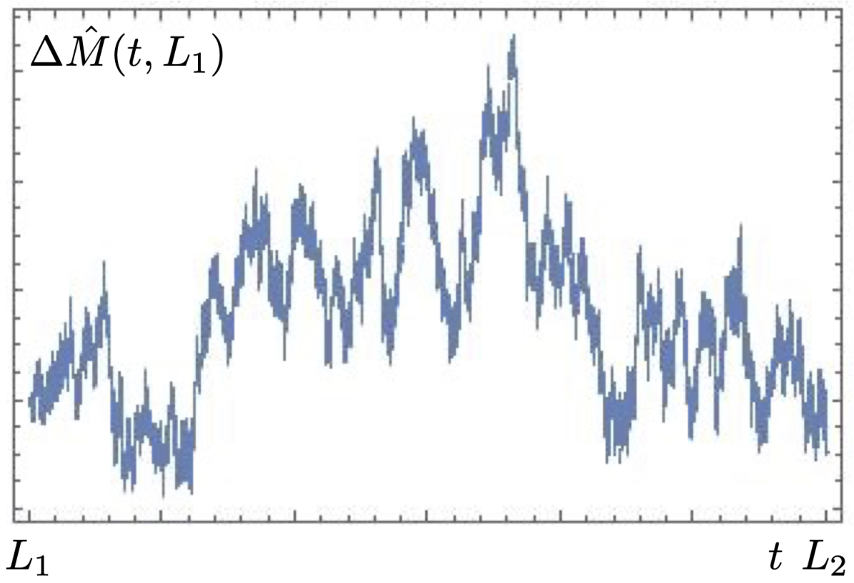
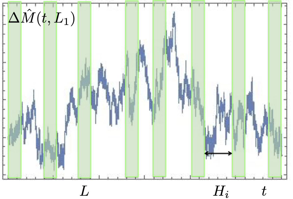
- 1.
Consider two very large integers and (which eventually we will send to infinity), with , but also .
- 2.
For any fixed integer , with , consider the union of sets
(179) made of non-overlapping and also well separated intervals of length whose origin is between the two large numbers and (see Figure 19). The integer is the cardinality of the set . These conditions ensure that the block variables computed on such disjoint intervals are very weakly correlated and therefore we can assume that we are dealing statistically with separated copies of the original series .
- 3.
At any given and , the cardinality of these sets cannot be larger of course than . There is however a large freedom in generating them:
- a
We can take, for instance, intervals separated by a fixed distance , with the condition that ;
- b
Alternatively, we can take, intervals separated by random distances such that .
- a
- 4.
The ensemble is then defined as the set of the block variables relative to the intervals :
(180)
In summary, choosing two very large and well separated integers and , we can generate a large number of sets of intervals and use the corresponding block variables of length to sample the typical values taken by a series consisting of a sum of consecutive terms . In view of the ergodicity, stationarity and scalability of the subsequences this is equivalent to determining the statistical properties of the original series .
XVI Frequency Tests
Starting with this section, we are going to present all statistical tests which we applied to check explicitly the randomness of our sequence . In this section we present the outputs of the simplest of these statistical checks which consist of frequency tests: we test, in order, the frequency of monobits, pairs, triplets, quadruplets and quintuplets. It is worth emphasizing that, in all cases, the null hypothesis of the random nature of the sequence has been confirmed with high confidence levels: for instance, in the case of the frequency test of the quintuplets, the pattern of 5 consecutive numbers such as along the sequence turns out to be as probable as or any of the other possibilities. It is worth saying that the successful outputs of our analysis emerged either applying the statistical tests to random subsets of the sequence , where we have made use of the intervals previously discussed, or to progressively increasing lengths of the sequence itself.
| sequence | random sequence | |||||||
|---|---|---|---|---|---|---|---|---|
| block | # 1 | # 0 | v | P-value | # 1 | # 0 | v | P-value |
| 1 | 9999306 | 10000694 | 0.98 | 0.33 | 10001800 | 9998200 | 0.80 | 0.42 |
| 2 | 9998263 | 10001737 | 0.77 | 0.43 | 10001502 | 9998498 | 0.67 | 0.50 |
| 3 | 10000928 | 9999072 | 0.41 | 0.67 | 9998258 | 10001742 | 0.78 | 0.43 |
| 4 | 10001456 | 9998544 | 0.65 | 0.51 | 10000964 | 9999036 | 0.43 | 0.67 |
| 5 | 9998082 | 10001918 | 0.85 | 0.39 | 9998122 | 10001878 | 0.83 | 0.40 |
| sequence | random sequence | |||||||
|---|---|---|---|---|---|---|---|---|
| L | # 1 | # 0 | v | P-value | # 1 | # 0 | v | P-value |
| 492 | 508 | 0.50 | 0.61 | 494 | 506 | 0.37 | 0.70 | |
| 4985 | 5015 | 0.30 | 0.76 | 4924 | 5076 | 1.52 | 0.12 | |
| 50006 | 49994 | 0.03 | 0.96 | 50019 | 49981 | 0.12 | 0.90 | |
| 500093 | 499907 | 0.18 | 0.85 | 499916 | 500084 | 0.17 | 0.86 | |
| 5000402 | 4999598 | 0.25 | 0.79 | 5000491 | 4999509 | 0.31 | 0.75 | |
| 50000577 | 49999423 | 0.11 | 0.90 | 50005027 | 49994973 | 1.00 | 0.31 | |
XVI.1 Monobit test
In this test we have checked the frequencies of the ’s and ’s along the sequence and compared this output with the corresponding frequencies of true random sequences. We have performed the analysis, choosing the variables . Defining
| (181) |
we take as the test statistic variable the absolute value of divided the square number of measurements2525 25 An alternative choice is to use the statistical test. We have also employed this test statistical variable, arriving to the same conclusions presented in the text.
| (182) |
In this test, the -value is given by eq. (171)
| (183) |
We have performed two types of analysis:
- 1.
In the first type of analysis we have chosen 5 random non-overlapping intervals with and . The results of this analysis, together with the value of and the -value, is reported in Table 6. In the same table, for a direct comparison we have also reported the corresponding data of a random sequence. One can see that there were always very high -values, i.e. our sequence passes successfully this statistical test.
- 2.
We have made the same statistical analysis but including progressively more and more terms in the sequence. The results are shown in Table 7. Also in this case there were always very high -values, i.e. our sequence passes successfully this statistical test.
| block | P-value | |||||
|---|---|---|---|---|---|---|
| 1 | 0.12504 | 0.12501 | 0.12497 | 0.12497 | 0.51 | 0.91 |
| 2 | 0.12496 | 0.12496 | 0.12500 | 0.12508 | 1.55 | 0.67 |
| 3 | 0.12503 | 0.12499 | 0.12500 | 0.12498 | 0.19 | 0.97 |
| 4 | 0.12505 | 0.12492 | 0.12506 | 0.12497 | 2.08 | 0.55 |
| 5 | 0.12498 | 0.12489 | 0.12502 | 0.12511 | 3.97 | 0.26 |
| L | P-value | |||||
|---|---|---|---|---|---|---|
| 0.1264 | 0.12480 | 0.1254 | 0.12330 | 1.33 | 0.72 | |
| 0.12496 | 0.12496 | 0.12500 | 0.12508 | 0.40 | 0.93 | |
| 0.12553 | 0.12447 | 0.12546 | 0.12453 | 0.79 | 0.85 | |
| 0.12480 | 0.12528 | 0.12545 | 0.12537 | 3.72 | 0.29 | |
| 0.12512 | 0.12496 | 0.12491 | 0.12501 | 1.85 | 0.60 | |
| 0.12499 | 0.12502 | 0.12496 | 0.12502 | 1.84 | 0.60 |
XVI.2 Pair frequencies
In this test we have analysed the frequency distribution of the pair along our sequence . There could be possible outputs, given by
| (184) |
If the sequence is random, the frequencies of each of these outputs must be . In this case, our test statistical variable is the chi-square
| (185) |
where is the measured frequency of each output given in (184) and the -value is given by the formula (170), i.e.
| (186) |
As before, we show the results of our analysis for five random blocks of length (see Table 8), in the interval , and for blocks of increasing lengths, starting from (see Table 9). Also in this case, the higher values of the -values shows that our sequence passes successfully also this test.
| block | P-value | |||||||||
|---|---|---|---|---|---|---|---|---|---|---|
| 1 | 4.165 | 4.168 | 4.166 | 4.173 | 4.165 | 4.161 | 4.166 | 4.167 | 3.89 | 0.79 |
| 2 | 4.165 | 4.168. | 4.166 | 4.163 | 4.166 | 4.169 | 4.167 | 4.167 | 1.47 | 0.98 |
| 3 | 4.160 | 4.165 | 4.167 | 4.174 | 4.166 | 4.168 | 4.166 | 4.166 | 4.87 | 0.67 |
| 4 | 4.170 | 4.163 | 4.177 | 4.161 | 4.171 | 4.160 | 4.161 | 4.165 | 13.7 | 0.05 |
| 5 | 4.162 | 4.170 | 4.170 | 4.168 | 4.162 | 4.166 | 4.169 | 4.163 | 3.68 | 0.81 |
XVI.3 Triplet frequencies
In this test we have analysed the frequency distribution of the triplets along our sequence . There could be possible outputs, given by
| (187) | |||
If the sequence is random, the frequencies of each of these outputs must be . In this case, our test statistical variable is the chi-square
| (188) |
where is the measured frequency of each output given in (187) and the -value is given by the formula (170), i.e.
| (189) |
As before, we show the results of our analysis for five random blocks of length (see Table 10) and, also for the triplets, the values of the -values show that our sequence passes successfully this test.

XVI.4 Quadruplet and quintuplet frequencies
For the statistical analysis of quadruplets and quintuplets it becomes rather cumbersome to show all the frequencies of the relative outcomes (there are outputs for the quadruplets and for the quintuplets). Hence, we simply decide to show in Figure 20 the histograms of the quadruplet and quintuplet frequencies for a block variable of length extracted around and, from these histograms, one can see a perfect balance among all frequencies of the events. We also report in Table 11 the values (given by eq. (166), with and ) and the -values for the frequency distribution of the quadruplets for blocks of increasing length , with . The same for the quintuplets, whose chi-square is computed according to eq. (166) with and , and with all relative data reported in Table 11. Also in these case, the higher values of the -values do not indicate a deviation of randomness of the sequence .
XVII Proportion of sequences passing a test
We can have an additional control on the significance of a statistical test we have done by computing the proportion of the results that pass the test2626 26 We strongly advice the reader to read Section 4.2 of the NIST report Nist for further details. on this topic.. We illustrate here the result for one particular test but we have checked that the same conclusions also apply to all other tests discussed in this part of the paper. Consider, for instance, the test about the equidistribution of triplets along the sequence . The protocol of the procedure is as follows
|
|
- 1.
For our sequence we consider non-overlapping intervals of length with increasing starting points (see eq.(174)). Associated to each of these intervals, there are subsequences of , each of length . We compute the frequencies of the various triplets in each of these subsequences and we compute the relative -values. Considered altogether, these steps form what we call a sweep.
- 2.
We compute the proportion of subsequences that pass the test. In our case, having fixed , we count the number of subsequences for which the -values .
- 3.
We repeat the sweep of point 1 for another times, choosing, each time, intervals of length never overlapping with any previous one.
- 4.
There is now a statistical formula Nist which determines the range of acceptable proportions in terms of the confidence interval: this is given by
(190) where is the sample size, sufficiently high in order to have a reasonable statistics (say ). Note that as the sample size , as expected.
- 5.
If the proportion falls outside this interval, then there is evidence that the data is non-random.
As our example we have chosen , and . So, in our case, the confidence interval is given by and . In Figure 21.a we show the result of this type of check for the triplets and all proportions are perfectly within the confidence interval. Similar results also hold for the tests concerning monobits, pairs, quadruplets and quintuplets.
XVII.1 Uniform distribution of P-values
One can also check the uniform distribution of the -values. This is easily done using a histogram of the various values obtained for the -values with the interval divided into 10 sub-intervals, with the relative counting of how many -values lie within each sub-interval. The quantitative degree of uniformity can be controlled in terms of a test, in this case given by
| (191) |
where is the sample size and are the frequencies of the -values relative to each interval. We can now calculate a -value for this distribution of the P-values! Let’s denote it by : it is associated to the of (191) and it is given by
| (192) |
According to Nist, if , then the sequences can be considered to be uniformly distributed. In Figure 21.b we report a typical histogram of the -values for one of our sweeps of the triplet frequencies, with the corresponding value equal to and therefore satisfies the bound for a uniform distribution of the -values.

XVIII Correlation function and discrete Fourier transform
Let’s consider a generic time series whose generic output is here denoted . Useful information on the nature of this time series can be obtained by computing the correlation between the two outputs and , where the interval is called the lag. For a sequence of length , the correlation function of lag is defined as
| (193) |
where is the average of the sequence . If we now take as time series our sequence , we can refine our definition of the correlation function and take as definition the quantity
| (194) |
where the average is taken wrt our stroboscopic sampling of our sequence . This means that we consider non overlapping intervals randomly chosen, with , and, in each of these intervals, we consider a sub-interval of length randomly chosen to extract a subsequence and to compute . Finally we average on all the ’s computed in this way. In our analysis we have typically chosen and .
For an infinitely long ideal true random sequence (i.e. ) it holds
| (195) |
However, our definition involves a finite sequence of length : in this case, for uncorrelated quantities of length , due to finite-size effects we expect that the variance of the sequence of the is instead of the order . This is indeed what is shown in Figure 22.a and 22.b, while the finite size scaling of the variance with respect to is show in Figure 22.c.
The Discrete Fourier transform of the correlation function is defined as
| (196) |
and its eventual peaks provide an indication of the periodicities present in the sequence. If was a true random sequence, would be a constant function of value . As shown in Figure 22.d, for our sequence the squared magnitudes of the discrete Fourier transform is a function almost constant around the expected value , with a spread due to the finite length of the sequences analyzed.

XVIII.1 Discrete Fourier Transform Test
The purpose of this test is to study the peak heights in the Discrete Fourier Transform of our sequence in order to detect, if any, its periodic features. The presence of these periodic features would indicate in fact a deviation from the randomness. We focus our attention to detect whether the number of peaks exceeding of the threshold value (given below) is significantly different than . The way the test is implemented is as follows
- 1.
Within a large interval around and , we select randomly intervals associated to subsequences of length of our sequence . In more detail, we have taken , , with .
- 2.
We compute the Discrete Fourier Transform of the subsequence made of consecutive restricted Möbius coefficients.
- 3.
We calculate the modulus of the first elements of the Discrete Fourier Transform.
- 4.
We compute the threshold value
(197) (for instance, in our case ). This is the peak height threshold value. If the sequence is random, of the values of should not exceed .
- 5.
We define the quantity , which is the expected () theoretical number of peaks that have to be less than the threshold if the sequence is random.
- 6.
We count , i.e. the actual observed number of peaks in that are less than and compute the statistical test
(198) - 7.
Then we compute the -value of this test, given by
(199) - 8.
If the computed -value is , then the sequence is not random.
A typical output of this test is shown in Figure 23.a, where we also show (the red dashed line) the threshold value . We perform our tests on sequences made of consecutive numbers chosen randomly among some stroboscopic large intervals of the overall sequence (with initial point of our analysis , see Section XV.6), always obtaining -values larger than the decisional value . Hence the sequence passes successfully also this test. A histogram of the -values we obtain is shown in Figure 23.b.

XVIII.2 Correlation with random vectors
As stated in Iwaniec, Green-Tao, the randomness of the Möbius coefficients would imply that they do not correlate with any reasonable sequence . In our case we can reformulate this statement as follows: (a) first of all we focus our attention to the restricted values of the Möbius function to square-free numbers only, i.e. the sequence ; (b) secondly, we extract a random consecutive sequence of values from this sequence; (c) thirdly, we compute the correlation of this sequence with another sequence made of values. This ends up in the formula
| (200) |
where means that, for , . In Figure 24 we present the correlation of versus with six random sequences made of : all these correlations seem not to grow faster than , so that the asymptotic behaviour dictated by (200) seems to be indeed “experimentally” well verified.
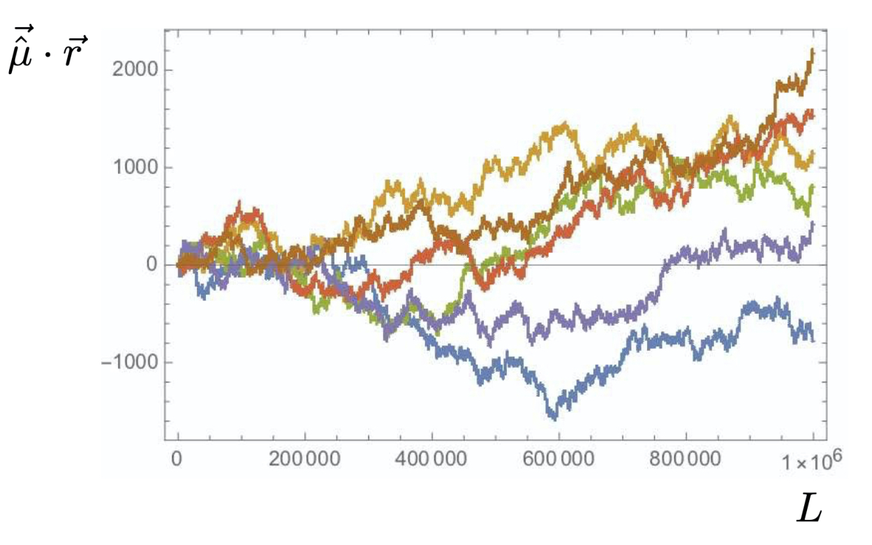
XIX Oscillation and long run of ones tests
In this chapter we address two more refined tests concerning the randomness of our sequence : the first concerns the variation of the ’s and ’s present in it, the second the longest strings of these symbols.
XIX.1 Oscillation test
Let’s consider the oscillations of our sequence and their statistics. An oscillation is considered to be a change from a 1 to 0 and vice versa. So, for instance, in this short piece of a sequence
the oscillations are in coincidence with the vertical bar hereafter
We are in presence of a fast oscillation when there are a lot of changes. To have a quick birds-eye view of the configurations, it is convenient to adopt a binary graphical notation, in which a black box is associated to while a white box is associated to . For instance, the alternating sequence
(which has the highest possible oscillation), has the graphical representation
while a sequence as
which has just one oscillation, graphically appears as
In statistical mechanics, if and denote the two ground states of an Ising like system, each oscillation corresponds to a kink state which interpolates between the ground states.
XIX.2 Bernoulli variables
In order to set up a statistical test for the oscillations, let’s fix some notation and some basic relations: hereafter (with ) denotes the -th element of a sub-sequence of , while and respectively denote the number of ’s and ’s in this sub-sequence. Therefore we have
| (201) |
In the following we denote by the fraction of ’s present in the sequence
| (202) |
Let’s also define the variable as
| (203) |
Then we can set up our statistical test in terms of the oscillations present in the sequence, defined as
| (204) |
simply measures the number of kinks (oscillations) present in the system: a large value of indicates that there are fast oscillations in the sequence while a small value that there are oscillations that are too slow. Both cases are not typical for a true random sequence.
The quantity is a Bernoulli variable with parameter , since we have
| (205) |
Hence, takes value only in the two cases in the middle and their probability is then . Therefore
| (206) |
Since is a linear combination of the variables we have
| (207) |
For its variance we have
| (208) |
where
| (209) | |||||
For the cases in which we have
| (210) |
while for the remaining cases where we have
| (211) |


Hence, putting all the pieces together, we have
| (212) |
In light of the formulas given above, in the limit where it is natural to define the normalized variable
| (213) |
and compute the P-value according to
| (214) |
If the computed -value is the sequence has to be considered non-random, otherwise the sequence is promoted to be random.
We have applied this test to sequences of consecutive values of taken randomly from different non-overlapping stroboscopic intervals of length , where . The result of this analysis is reported in Figure 25, where in Figure 25.a we show the histogram of the numbers of values of obtained in our test while in Figure 25.b we show the value obtained in each sweep, together with the intervals relative to , and standard deviations. Although most of the values are within standard deviations, there are few of them which fall beyond standard deviations, with a -value which was below . Are these deviations significant or are just statistical fluctuations? To answer this question, we have performed the analysis of the proportion of sequences passing the test: using blocks of sweeps each, we compute the proportion of sequences which pass the test, with the range of acceptable proportion determined by eq. (190), with . Hence, in this case . The relative histogram of all obtained -values is reported in Figure 26.a, while the proportion of sequences passing the test is in Figure 26.b, in which we see that the few cases which have -values lower than the threshold can be considered statistical fluctuations.
XIX.3 Longest Run of ’s
The purpose of this test is to check whether the length of the longest run of ’s is compatible with the length expected in a true random sequence. Of course irregular patterns in the longest runs of ’s also implies irregular patterns in the longest runs of ’s. To perform such a test, first of all we sample stroboscopically our sequence in terms of our intervals . Then, in each interval we extract a subsequence2727 27 The lengths of the variables , , and are fixed in these amounts by the request to optimise the statistical test, see Nist. of consecutive values from ; we divide such a subsequence in -bit blocks (which we take here to be ) and we measure how all the observed longest run length within the -bit blocks matches the expected longest length within -bit blocks. We take the following categories of events , for which is known their relative tabulated probabilities (see Table 12) Nist. In this case the corresponding variable is given by
| (215) |
where , with the -value given by
| (216) |
The relative data, reported in Figure 27, shows that the sequence also passes successfully this test.
| 0.1174 | |
| 0.2430 | |
| 0.2493 | |
| 0.1752 | |
| 0.1027 | |
| 0.1124 |
XX Non-overlapping matching test
We can screen our sequence for the number of occurrences of a given pre-defined aperiodic target -bit string and compare the actual frequency of this string with its theoretical probability. In more detail, the purpose of this test is to detect whether there are too many or less sequences than expected. In other words, this test rejects sequences which exhibits irregular occurrences of a given a-periodic pattern. The protocol goes as follows Barbour:
- •
we extract a subsequence from . Such a subsequence is made of the union of neighborhood blocks of length .
- •
we denote by () the number of times that the target string occurs within the block . The search for matches proceeds by creating an -window on the sequence, comparing the bits within that window against the target .
- •
if there is no match, the window slides over one bit. If there is instead a match, the window slides over bits.
- •
at the end of the process, for each block we see the final values of the variables .
Under the hypothesis of the randomness of the sequence, the expected mean and variance of the variable are Nist
| (217) |
Hence, the variable is defined as
| (218) |
and the corresponding -value is therefore given by
| (219) |
Before presenting our data, an example will help in clarifying the nature of this test.
Example. Let’s choose and , with and target -string . Let’s imagine that our subsequence is
| (220) |
made of blocks of length
| (221) |
As we stated, as target string we choose . Hence we have the situation shown in the Table 13. Therefore, for this example, we have
| (222) | |||||
| (223) |
The variable is then
| (224) |
and the corresponding -value is
| (225) |

| Block 1 | Block 2 | |||
| Bit Positions | Bits | Bits | ||
| 1-3 | 100 | 0 | 010 | 0 |
| 2-4 | 001 (hit) | 1 | 010 | 0 |
| 3-5 | Not examined | 000 | 0 | |
| 4-6 | Not examined | 001 (hit) | 1 | |
| 5-7 | 000 | 1 | Not examined | |
| 6-8 | 001 (hit) | 2 | Not examined | |
| 7-9 | Not examined | 100 | 1 | |
| 8-10 | Not examined | 001 (hit) | 2 | |
| Total | 2 | 2 | ||
Results for the sequence . In implementing this test on our sequence we have chosen an aperiodic string of bits, in particular we have employed the target string
| (226) |
as well as other target strings such as
| (227) |
We have always chosen blocks of length in sequences extracted randomly in the interval of values of the sequence given by . The number of subsequences analysed were . The data relative to the P-values and the proportions of them that pass the statistical test are reported in Figure 28: from these plots one can see that our sequence passes successfully also this non-overlapping matching test.
XXI Rank of matrices
Among the different tests which we can make to verify the randomness of our sequence , one of them concerns the distribution of the rank of binary matrices that can be built up in terms of the elements . The test goes as follows Marsaglia: given an integer length (in our case ) and a segment of length of our sequence , we have disjoint blocks of : each of them can be rearranged in such a way to form a binary matrix. Each row of these matrices is filled with successive terms of the original sequence (see Figure 29). Once we have organized our original segment of of length in this way, we can enquire about the probability distribution of the ranks of these matrices on the binary field : this means that, denoting by either the -th binary row or column of these matrices, we can make linear combinations of these vectors but only using as coefficients the two elements of
| (228) |


XXI.1 Probability of the ranks
For a purely random binary matrix, after making properly linear combination of the rows, its rank is essentially the number of nonzero rows and this can be determined by a simple counting. Hence, the probability that the rank of a random binary matrix takes the value is given by MarsagliaTsay
| (229) |
Surprisingly enough, the maximum of this probability distribution is not at but at : this is easily seen taken limit, where we have
| (230) | |||||
and the rest of all other probabilities having very small values () when . Below we denote by the probability relative to all other ranks but and , i.e .
XXI.2 Protocol
As usual, we have stroboscopically extracted from our sequence various subsequences of length in terms of the intervals . Here we present the result relative to intervals of length around both for matrices with and . When , we have a sample of matrices while, when , we have a sample of matrices. For each interval, we have determined the rank of each matrix and the frequencies , and of the values , and the ranks not exceeding
The chi-square value is easily defined
| (231) |
In Figure 30 we report the distribution of the P-values and the proportions of the subsequences which are within the interval of confidence for the case (for the results are analogous). In both cases analysed ( and ), our sequence has successfully passed this test.
XXII Maurer Universal statistical test
A non-random sequence has a certain level of predictability. This permits to compress the sequence without losing information: this idea is at the basis of all file compression, irrespectively of whether they are text files, video or audio files. On the other hand, a purely random sequence presents a “strong resistance” to its compression, because there are no periodic or predictive patterns that can be used to this aim. Therefore, the stronger is the resistance of a sequence to its compression, the higher is its level of randomness.

The purpose of the Maurer Universal statistical test is to detect whether or not a sequence can be significantly compressed keeping its level of information. The protocol goes as follows Maurer:
- •
we denote by the sum of the distances between matching -bit templates, i.e. the sum of the number of digits in the distance between -bit templates.
- •
we consider a sub-sequence of length extracted from our sequence and divided into two segments: an initialization segment made of non-overlapping blocks of length , and a test segment of non-overlapping blocks also of length , as shown in Figure 31.
As an example, let’s assume that , so that . Assume that and , so that . The initialization segment is , while the test segment is . The -bit blocks are shown in the following Table
Type Block Contents 1 10 Initialization 2 01 Segment 3 00 4 01 5 10 Test 6 01 Segment 7 00 8 00 9 11 10 01 - •
We can use the initialization segment to create a table for each possible -bit value, namely the -bit value is used as an index for the table. The block number of the last occurrence of each -bit block is noted in the table, with the rule that the index goes from to , where , where is the decimal representation of the content of the -th -bit block.
Following the example above, the following Table is created in terms of the initialization blocks
Possible M-bit Value 00 01 10 11 (saved in (saved in ) (saved in ) (saved in ) Initialization 3 4 1 0 - •
We then examine each of the blocks in the test segment and determine the number of blocks since the last occurrence of the same -bit block (i.e. ). Replace the value in the table with the location of the current block (i.e. ). Add the calculated distance between re-occurrences of the same -bit block to an accumulating sum of all the differences detected in the blocks, namely .
Following the example given above, the table and the cumulative sum are constructed as follows:
- –
For block 5 (i.e. the first test block): 5 is placed in the “10” row of the table (i.e. , and
- –
For block 6: 6 is placed in the “01” row of the table (i.e. ) and
- –
For block 7: 7 is placed in the “00” row of the table (i.e. ) and .
- –
For block 8: 8 is placed in the “00” row of the table and .
- –
For block 9: 9 is placed in the “11” row of the table (i.e. ) and .
- –
For block 10: 10 is placed in the “01” row of the table and
. The states of the Table are given by
Iteration Possible M-bit Value Blocks 00 01 10 11 4 3 4 1 0 5 3 4 5 0 6 3 6 5 0 7 7 6 5 0 8 8 6 5 0 9 8 6 5 9 10 8 10 5 9 - –
- •
We compute the test statistic variable
(232) where is the table entry corresponding to the decimal representation of the content of the -th M-bit block. In our example, .
- •
We then compute the -value, given in this case by
(233) where and are the theoretical expected values for the mean and the variance of the variable . These quantities are tabulated for different values of and Nist. Since, in our case, we decide to use , and (these numbers somehow optimize the performance of the test), the theoretical mean and the standard deviation are given by
(234)
We have performed our test on sequences of total length extracted from our original sequence in the interval . The histogram of the -values and the proportions of the sequences that pass the statistical test are shown in Figure 32. These plots show that our sequence successfully passes also this Maurer Universal Statistical Test. This means that our sequence cannot be compressed significantly without losing information2828 28 The same conclusion is also reached using standard file compression applications implemented on Mac: applied to large sequences extracted by , the compressed files had sizes equal to of the original files. Whoever is interested in performing such a kind of test can request a sample of these sequences by writing to one of us..

XXIII Entropy test
How unpredictable is our sequence ? To answer this question, we are going to test the frequency of all possible overlapping -bit pattern across the entire sequence. The aim of this statistical test is to compare the frequency of overlapping blocks of two consecutive/adjacent lengths ( and ) against the expected result for a purely random sequence. In the following we denote with the subsequence of to be tested of length . The protocol goes as follows Pincus:
- 1.
Given the sequence , we create another one by appending bits from the beginning of the sequence to the end of the sequence.
So, for example, if (with ) and , we append the and at the beginning of to its end, giving rise to the new sequence .
- 2.
We make a frequency count of the overlapping blocks (if a block containing to is examined at time , the block containing to is examined at time ). We denote by the count of the possible -bit, where is the -bit value.
For the example above, the overlapping -bit blocks (here ) are: . The calculated counts for the possible -bit strings are
- 3.
We compute for each value of . For our example,
- 4.
We then compute
(235) For our example
- 5.
We then repeat steps 1-4 replacing with
Step 1: in our example, is now and the sequence to be tested become .
Step 2: the overlapping blocks become: 0110, 1100, 1001, 0010, 0101, 1010, 0101, 1010, 1011. The calculated values are
and all the other patterns values are zero.
Step 3. Hence we have
Step 4. Hence we have
- 6.
Since for a fixed block length it is expected that in long random irregular strings, one has
the limiting distribution of the variable
(236) should coincide with that of a -random variable with degrees of freedom. Therefore the -value is given by
(237) In our example, and
We have performed the entropy test on subsequences of length in the interval with a pattern of -bits. The results of the statistical analysis are reported in Figure 33 and so, our sequence passes successfully also this test.

XXIV Cumulative sum Test
The aim of this test is to analyze the maximal excursion (from zero) of the random walk defined by the cumulative sum of the subsequences of with values . The feature under scrutiny is whether the cumulative sum of the partial sequences occurring in the tested sequence is too large or too small with respect to the expected behaviour of the cumulative sum of a purely random walk. While for a random sequence, the excursion of the random walk should be near to zero, for non-random sequences one expects that the excursion from zero may be significant. The theoretical framework behind this test is the standard random walk (see, for instance Yuval, Mazo, Rudnick, Levy, diffusion).
To implement this test let’s consider the block variables, defined earlier in eq.(177)
| (238) |
The statistical variable of the test is
| (239) |
i.e. the largest of the absolute values of the partial sums . From the theory of the random walk, the limiting distribution of the absolute values of the partial sum is
| (240) | |||
where, above, is the standard function
| (241) |
The corresponding -value is given by
| (242) |
We have analyzed subsequences of length in the interval and the histogram of the corresponding -values are reported in Figure 34, together with the proportion of the sequences that pass the statistical test -value . Also in this case, the conclusion is that the sequence passes successfully this test.

XXV Random Excursions Test
In this test we consider the subsequences with values and we test them versus certain predictions which come from purely random walk theory. The protocol of this test is as follows baron:

| Cycles | |||
| State | Cycle 1 | Cycle 2 | Cycle 3 |
| x | (0,1,0) | (0,-1,-2,-1,0) | (0,1,2,1,2,0) |
| -4 | 0 | 0 | 0 |
| -3 | 0 | 0 | 0 |
| -2 | 0 | 1 | 0 |
| -1 | 0 | 2 | 0 |
| 1 | 1 | 0 | 2 |
| 2 | 0 | 0 | 2 |
| 3 | 0 | 0 | 0 |
| 4 | 0 | 0 | 0 |
- 1.
we consider a subsequence of length extracted from the sequence .
- 2.
we consider the partial sums of our sequence. We denote by the total sum where we have added zeros before and after , i.e. .
- 3.
we count the number of zero crossings in , where a zero crossing is a value of zero in that occurs after the starting point. is also the number of cycles in , where a cycle of is a subsequence of consisting of an occurrence of zero, followed by no-zero values and ending with another zero. Of course the ending zero in one cycle may the beginning zero in another cycle. For statistical reasons which will explain better below2929 29 For a test, the number of variables must be at least larger than and this is the reason of the constraint on ., we have to be sure than the number of zeros in the sequence is larger than 800. Looking at the Figure 35, in the plot there are cycles given by the sequences (0, 1,0), (0,-1,-2,-1,0) and (0,1,2,1,2,0).
- 4.
- 5.
for each of the eight states of , we compute = the total number of cycles in which state occurs exactly times among all cycles, for (for , all frequencies are stored in ). We have the sum rule . For the example of Figure 35, the situation is summarised in Table 15.
Number of Cycles State x 0 1 2 3 4 5 -4 3 0 0 0 0 0 -3 3 0 0 0 0 0 -2 2 1 0 0 0 0 -1 1 0 1 0 0 0 1 1 1 1 0 0 0 2 2 1 0 0 0 0 3 3 0 0 0 0 0 4 3 0 0 0 0 0 Table 15: Occurrence of the various values in each cycle. 
Figure 36: (a) Histogram of the -values for the Cumulative Sums () for sequences (b) Proportions of sequence that pass the statistical test -value . In red the lower and higher values of the confidence interval. - 6.
The theoretical prediction of these frequencies (here denoted as ) are known baron and are given by
(243) - 7.
Using these theoretical and the observed frequencies we can define the variables (for each value ), given by
(244) This variable is expected to have a -distribution with degrees of freedom. This is valid as far as . Since (corresponding to , this lead us to the constraint on and to the necessity take into consideration only those sequences with .
- 8.
The corresponding -value of this test is given by
(245)
Here we present in Figure 36 the distribution of the -value for since all other values present similar behaviour. We have analyzed non-overlapping subsequences of length extracted by the sequence in the interval . As evident from Figure 36, our sequence passes successfully also this test.
XXVI Time distribution tests
Consider a true one-dimensional random walk (see Figure 37) whose starting point is at the origin and which is long . In the interval we can identify the time in which the random walk reaches its maximum and the time in which it reaches its minimum. In the following we denote by the time interval between the maximum and the minimum, .

XXVI.1 Probability distribution of and
The probability distributions and are exactly known for the pure random walk case Feller, Yuval: first of all, for symmetry reasons, they are equal and given by
| (246) |
where is the scaling variable . The distribution is symmetric with respect and its first moments are
| (247) |
We have sampled many different intervals of the sequence and compared the experimental distribution of versus the theoretical one given in eq. (246). Here we show the result relative to an interval of values around : we have divided this interval into segments of length and for each of these intervals we have determined . The comparison between the theoretical and experimental distributions are shown in Figure 38: the variable of this example is (for degrees of freedom) and the relative -value =, confirming the matching between the distribution coming from random walk and Mertens function. The experimental values of the first moments for the data shown in Figure 38 are
| (248) | |||
which differ just of few percents from the theoretical ones. We have also performed the Kolgomorv-Smirnov test to check the goodness of the expected function (250) versus the data: with a sample of points, the Kolmogorov-Smirnov variable is defined as
| (249) |
where is the cumulative distribution function associated to (246) while is the “experimental” cumulative distribution function with points. In our case, and we got which gives a probability larger than that the experimental data follow indeed the expected theoretical function (246).


XXVI.2 Probability distribution of
Recently Mori et al. MoriMajumdar have determined the exact probability distribution of the time interval . Denoting this function as , it has the scaling form
| (250) |
where the exact expression of the scaling function is given by
| (251) |
As shown in MoriMajumdar, this scaling function satisfies the integral equation
| (252) |
| theoretical value | experimental value | relative error | |
|---|---|---|---|
which is extremely useful for computing the various moments of the scaling variable . Indeed, one has simply to expand both terms in powers of and compare the corresponding coefficients. In this way, the first exact expressions of the moments are
| (253) | |||||
where are the Riemann zeta function. The numerical value of other moments are reported in Table 16. Also in this case we have sampled many different intervals of the sequence and compared the experimental distribution of versus the theoretical one given in (251). Here we show the result relative to an interval of values around : we have divided this interval into segments of length and for each of these intervals we have determined . The comparison between the theoretical and experimental distributions are shown in Figure 39: the variable of this example is (with degrees of freedom) and the relative -value is -value equals , confirming the matching between the distribution coming from random walk and the Mertens function. Also in this case we have performed the Kolgomorv-Smirnov test to check the goodness of the expected function (250) versus the data: with a sample of points, the Kolmogorov-Smirnov variable is defined as usual as
| (254) |
where, in this case, is the cumulative distribution function associated to (250) while is the “experimental” cumulative distribution function with points. In our case, and we got which gives a probability larger than that the experimental data follow indeed the expected theoretical function (250). There is also an impressive agreement between the theoretical and the experimental values of the first ten moments as shown in Table 16.
XXVII Central limit theorem and a probabilistic conclusion on Mertens function
In light of all the successful outputs of all the statistical tests that we have presented so far, it must appear natural that the Mertens function has a probabilistic distribution given by the gaussian normal law.
As stressed several times, is completely deterministic with no probabilistic aspect per se. However, as explained in Section XV, one can generate an ensemble and study its probability distribution by taking “stroboscopic images” of this quantity. To this aim, we need to adopt the block variables previously defined, see eq. (177): these block variables are parts of the Mertens function and provide stroboscopic images of this function. These quantities are the analog of the stroboscopic images which are needed to address the single Brownian motion problem Yuval, Mazo, Rudnick, Levy, diffusion.
The original interval relative to the start and ending points of the series can be broken into a large set of non-overlapping and well separated intervals of length , of which we compute the corresponding block variables : it is this collection of block variables that forms the set of events, i.e. the ensemble relative to the sums of consecutive terms (see Section XV.7)
| (255) |
Of course, given the infinite sequence of the Möbius coefficients, we could systematically enlarge the interval , with , and take as new block variables those with length equal to the length of the original series , and keep going with and so on and so forth. Hence, with the ensemble defined as in eq. (180), i.e. made of non-overlapping and well separated intervals of length , we compute the corresponding block variables of these intervals and sample them. Based on the exact result of vanishing mean of the sequence and the absence of correlation between the restricted Möbius coeffients coming from the statistical analysis done in the previous sections
| (256) |
we expect that the probability distribution of the random quantity
| (257) |
associated to the block variables is just given by the normal distribution
| (258) |
This is clearly seen in Figure 40, where we show a histogram relative to one of the samplings described above vs the normal distribution law . The conclusion that the sampling of the restricted Mertens function satisfied the normal distribution is well supported by a large set of appropriate P-values of standard numerical analysis tests, such as Anderson-Darling, Cramer-von Mises, Pearson , etc. We have also performed the Kolgomorov-Smirnov test relative to sampling point and we got for (see eq. (249) for the definition of ), which gives a probability larger than than the data follow indeed a normal law distribution.

It is well understood that the above gaussian distribution does not imply that . In fact, the random walk behavior behind the gaussian distribution is known to imply
| (259) |
For the remainder of this section, we describe two ways to deal with this fact as far as attempting to address the GRH based on (258).
First, based on the above normal distribution, the block variables of length always scale as for arbitrarily small . In probabilistic language, in the limit this behavior occurs with probability equal to 1. Indeed, using the gaussian distribution (258), in the limit we have
| (260) | |||||
Chose for any . Then for any ,
| (261) |
It is important to note that the above probability is not equal to as if . Since every element in the set behaves the same as far as its growth is concerned, the almost surely true probabilistic statement above, meaning with probability equal to , is promoted to the surely true statement that
| (262) |
without assuming the RH.
A second and more detailed approach is also based on the above results. Based on the above normal law, one can place a different kind of bound not involving the above , by invoking the law of iterated logs. If, as argued above, is a random walk, then the law states
| (263) |
where means almost surely. As stated above, the bound (263) is sufficient for showing the validity of the GRH since the ’s do not spoil convergence of the integral (8). The analysis done for the block variables which sample on all possible scales the restricted Mertens function extends of course to itself, so that we can conclude
| (264) |
PART D
XXVIII Conclusions
There are different ways to approach the Riemann Hypothesis, as discussed for instance in Borwein. In this paper, we have pursued an approach which consists of identifying the first singularity, approaching the critical line from the right, of the inverse Mellin transform of the restricted Mertens function for the square-free numbers . Such a function is a sum of terms relative to the Möbius coefficients of the square-free numbers. Our efforts in this paper have been to show the stochastic behaviour of the restricted Mertens function , despite its deterministic nature. To this aim, we have developed a global approach to the function based on a series of probabilistic results concerning the prime number distribution along the series of square-free numbers, the average number of prime divisors, the Erdős-Kac theorem for square-free numbers, etc. All these results support the existence of a normal law satisfied by .
It is better to stress once again that there is nothing which prevents a deterministic sequence from being a realization of a random process, and the restricted Möbius coefficients and the associated Mertens function seem to be a very good example of this fact. This has been strikingly confirmed by our further numerical analysis aimed to check the local stochasticity of the restricted Möbius coefficients. Indeed, driven by the natural curiosity to see how good the random nature of the Mertens function and its Möbius coefficients is satisfied by finite samples of these sequence, we have performed a massive statistical analysis in a range up to natural numbers, applying numerous randomness tests of increasing precision and complexity: all these tests were successfully satisfied with a level of reliability of , as quantified by the chi-square distributions.
For a theoretical physicist, all these results leave essentially no room to doubt the validity of the Riemann Hypothesis: the probabilistic approach pursued here has led to the conclusion that
| (265) |
This is a probabilistic result that applies to all random sequences made of , therefore also to the Mertens function once its random nature has been established. We expect that our bound (265) is the best one can obtain for the Mertens function without assuming the RH: as a matter of fact, in this paper we have reversed the argument, i.e. we have shown that we can use the bound (265) to arrive to the validity of the RH. The successful outputs of all the statistical tests performed in this paper show that the sequence of the Möbius coefficients , restricted to the square-free numbers, is, for all practical purposes, a random sequence and it can be used as a perfect random number generator in any computer simulation, an interesting by-product of our analysis.
However, putting aside any probabilistic considerations, one may be curious about the asymptotic behavior of the actual Mertens function . As easily imagined, this behavior is presently unknown but an estimate of the asymptotic behaviour of this function can be achieved assuming the validity of the Riemann Hypothesis. This is, for instance, the content of a series of bounds obtained by various authors. Let’s define
| (266) | |||
Soundararajan, for instance, assuming the RH, arrived to the bound SounMert, Balazard
| (267) |
A more stringent bound comes from an unpublished conjecture by Gonek Gonek1, who stated that
| (268) |
The above bound remains an unpublished conjecture, however further evidence for it was given by Ng Ng, and it is likely to be correct. Notice that, if it is indeed correct, it does not contradict the bound (265) which was based on the normal distribution we described in this paper. As a matter of fact, the probability estimate of the (restricted) Mertens function based on the law of iterated logs described in this paper satisfies the inequalities
| (269) |
for large , and it is therefore in agreement with both bounds.
In this paper we have also argued that the validity of the RH can imply the validity of the GRH, and we have argued this on the basis of two hypotheses: (i) that the restricted Mertens function goes as and (ii) that the restricted Möbius coefficients behave as random independent variables. Both hypotheses seem indeed satisfied. It would be of course interesting to find an alternative proof of the inequality (95) based on a global analysis of the functions , similarly to the analysis done in Part B for the function .
In conclusion, using a probabilistic approach and the robustness of probabilistic theorems that followed, the validity of the Riemann and the Generalised Riemann Hypothesis comes quite naturally from the central limit theorem and the dominant role of the gaussian distribution law in the probabilistic realms. Even taking a more conservative point of view, it remains however true that, in view of the large battery of analytic results and statistical tests here presented, while a violation of the RH may be still possible, it is an event which appears however to be wildly improbable.
Acknowledgements
We would like to thank Andrea Gambassi, Steve Gonek, Satya Majumdar, Silvia Pappalardi, Kannan Soundararajan and Don Zagier for useful discussions on different aspects of the problem. We are particularly grateful to German Sierra for his suggestions and a thorough and deep reading of the manuscript. This work has been carried on for several years, during which we have enjoyed the hospitality of several institutes. GM would like to thank in particular: the Simons Center for Geometry and Physics in Stony Brook, the International Institute of Physics in Natal and Institute Henri Poincare in Paris for the nice hospitality and partial support during part of this work. AL thank SISSA for the kind hospitality and partial support during the early stage of the work.
Appendix A The mean of the Mertens function
Let’s start from an identity which involves the Möbius coefficients , namely Apostol
| (270) |
where the sum over is made on the numbers which divide . This identity is important for proving that the mean of the Mertens function vanishes.
| (271) |
To prove this result, let’s start by showing that for any it holds
| (272) |
Consider the sum , which is of course equal to . Thanks to the identity (270), we can write as
| (273) | |||||
where and are respectively the integer and the fractional parts of the number . Using that if and the bound for all , for the last term we have and therefore
| (274) |
So, taking , we have indeed the bound (272). Consider now the function
| (275) |
and write the Mertens function as
| (276) |
namely
| (277) |
Taking , we have that since it is just the value of the Möbius function at , while for the second term, given an arbitrary , there exists a constant (which depends on ) such that if . Hence, we have
| (278) |
and thererfore, in the limit
| (279) |
Since can be arbitrarily small, we have then the prove of (271).
References
- [1] B. Riemann, On the number of primes less than a given magnitude, translated by H.M. Edwards, from Ueber die Anzahl der Primzahlen unter einer gegebenen Grösse (1859) in reference [3].
- [2] H.M. Edwards, Riemann Zeta Function, Academic Press, New York, 1974.
- [3] E.C. Titchmarsh, The Theory of the Riemann Zeta Function, Oxford Univ. Press, Oxford, 1986.
- [4] H. Davenport, Multiplicative Number Theory, Springer-Verlag, New York, 2000.
- [5] E. Bombieri, Problems of the Millennium: The Riemann Hypothesis, Clay Mathematics Institute, (2000).
- [6] P. Sarnak, Problems of the Millennium: The Riemann Hypothesis, Clay Mathematics Institute, (2004).
- [7] B. Conrey, The Riemann Hypothesis, Notices of AMS, March, 341 (2003).
- [8] G. Polya, unpublished (c. 1914). See A. Odlyzko, Correspondence about the origins of the Hilbert-Polya conjecture, http://www.dtc.umn.edu/odlyzko/polya/index.html (1981-1982).
- [9] P. Borwein, S. Choi, B. Rooney, A. Weirathmueller, The Riemann Hypothesis. A Resource for the Afficionado and Virtuoso Alike, Canadian Mathematical Society, Springer, 2008
- [10] K. Broughan, Equivalents of the Riemann Hypothesis, vol 1 and 2, Cambridge University Press 2017.
- [11] T.M. Apostol, Introduction to Analytic Number Theory, 5th edn. (Springer, New York, 1998).
- [12] H. Iwaniec and E. Kowalski, Analytic Number Theory, AMS Colloquium Publications 53, Providence, RI 2004.
- [13] E. Bombieri, The classical theory of Zeta and -functions, Milan J. Math. 78 (2010) 11–59.
- [14] J. Steuding, Value-Distribution of L-Functions, Springer-Verlag Berlin Heidelberg 2007.
- [15] H. Iwaniec, P. Sarnak, Perspectives on the analytic theory of -functions, GAFA, Geom. funct. anal. Special Volume (2000) 705–741
- [16] M. V. Berry, Riemann’s zeta function: a model for quantum chaos?, in Quantum Chaos and Statistical Nuclear Physics, edited by T. H. Seligman and H. Nishioka, Springer Lecture Notes in Physics Vol. 263 , p. 1, Springer, New York (1986).
- [17] M.V. Berry, Semiclassical formula for the number variance of the Riemann zeros, Nonlinearity 1 (1988), 399-407.
- [18] M.V. Berry, The Riemann-Siegel formula for the zeta function: high orders and remainders, Proc. Roy. Soc. Lond. A450, 439-462 (1995).
- [19] M.V. Berry, Quantum chaology, (the Bakerian lecture), Proc. Roy. Soc. London Ser. A, 413 (1987), 183-198.
- [20] M.V. Berry, J.P. Keating, and the Riemann zeros, in Supersymmetry and Trace Formulae: Chaos and Disorder, ed. J.P. Keating, D.E. Khmelnitskii and I. V. Lerner, Kluwer, 1999.
- [21] M. V. Berry, J. P. Keating, The Riemann zeros and eigenvalue asymptotics, SIAM Review 41, 236, 1999.
- [22] M. V. Berry and J. P. Keating, A compact hamiltonian with the same asymptotic mean spectral density as the Riemann zeros, J. Phys. A: Math. Theor. 44, 285203 (2011).
- [23] J. B. Bost and A. Connes, em Hecke Algebras, Type III factors and phase transitions with spontaneous symmetry breaking in number theory, Selecta Mathematica, New Series 1, No. 3 (1995), 411-457.
- [24] A. Connes, Trace formula in noncommutative geometry and the zeros of the Riemann zeta function, Selecta Mathematica New Series 5 29, (1999); math.NT/9811068.
- [25] J. Keating, N. Snaith, Random Matrix Theory and , Commun. Math. Phys. 214, 57 (2000).
- [26] G. Sierra and J. Rodriguez-Laguna, The model revisited and the Riemann zeros, Phys. rev. Lett. 106, 200201 (2011).
- [27] G. Sierra, The Riemann zeros as spectrum and the Riemann hypothesis, Symmetry 2019, 11(4), 494, and references therein
- [28] G. Sierra, A Physics pathway to the Riemann hypothesis, in ”Mathematical physics and field theory: Julio Abad, ”in Memoriam”. Eds. M. Asorey, J.V. Garcia Esteve, M.F. Ranada, J. Sesma, 2009, 978-84-92774-04-3 , pags. 383-390.
- [29] M. Srednicki, The Berry-Keating Hamiltonian and the Local Riemann Hypothesis, J. Phys. A: Math. Theor. 44 305202 (2011); arXiv:1104.1850.
- [30] C.M. Bender, D.C. Brody, M.P. Müller, Hamiltonian for the zeros of the Riemann zeta function, Phys. Rev. Lett. 118, 130201 (2017).
- [31] D. Schumayer, D. A. W. Hutchinson, Physics of the Riemann Hypothesis, Rev. Mod. Phys. 83, 307 (2011), and references therein.
- [32] M. Wolf, Will a physicist prove the Riemann hypothesis?, Rep. Prog. Phys. 83 (2020) 036001.
- [33] M. Griffin, K. Ono, L. Rolen, D. Zagier, Jensen polynomials for the Riemann zeta function and other sequences, Proc. Natl. Acad. Sci. U.S.A. 116, 11103 (2019)
- [34] B. Rodgers and T. Tao, The De Bruijn-Newman constant is non-negative, Forum of Mathematics, Pi, 8, E6. doi:10.1017/fmp.2020.6
- [35] G. França and A. LeClair, Transcendental equations satisfied by the individual zeros of Riemann zeta, Dirichlet and modular L-functions, Communications in Number Theory and Physics, Vol. 9, No. 1 (2015).
- [36] G.H. Hardy, (1914), Sur les Zeros de la Fonction de Riemann, C. R. Acad. Sci. Paris, 158: (1914), 1012.
- [37] N. Levinson, More than one-third of the zeros of Riemann’s zeta function are on , Adv. Math., 13 (1974), 383.
- [38] J.B Conrey, More than two fifths of the zeros of the Riemann zeta function are on the critical line, J. Reine Angew. Math., 1989 (399): 1-16,
- [39] A. Selberg, Contributions to the theory of Dirichlet’s -functions, Skr. Norske Vid. Akad. Oslo. I. 1946 (1946) 2–62
- [40] A. Fujii, On the zeros of Dirichlet -functions. I, Transactions of the American Math. Soc. 196 (1974) 225–235
- [41] H. Iwaniec, W. Luo, P. Sarnak, Low lying zeros of families of -functions, Publications mathématiques de l’I.H.E.S., ime 91 (2000), 55-131, arXiv:math/9901141 [math.NT] (1999)
- [42] C. P. Hughes, Z. Rudnick, Linear statistics of low-lying zeros of -functions, Quart. J. Math. 54 (2003) 309–333, arXiv:math/0208230v2 [math.NT]
- [43] J. B. Conrey, H. Iwaniec, K. Soundararajan, Critical zeros of Dirichlet -functions, arXiv:1105.1177 [math.NT] (2011)
- [44] E.C. Titchmarsh, (1936), The Zeros of the Riemann Zeta-Function, Proceedings of the Royal Society of London. Series A, Mathematical and Physical Sciences, The Royal Society, 157 (891): 261-263 (1936).
- [45] A. M. Turing, Some calculations of the Riemann zeta-function, Proceedings of the London Mathematical Society, Third Series, 3: 99-117 (1953).
- [46] J. van de Lune,. H.J.J. te Riele, D.T. Winter, On the zeros of the Riemann zeta function in the critical strip. IV, Mathematics of Computation, 46 (174): 667 (1986).
- [47] A.M. Odlyzko, The 1020-th zero of the Riemann zeta function and 175 million of its neighbors, unpublished report.
- [48] D. Platt, David and T. Trudgian, The Riemann hypothesis is true up to , arXiv:2004.09765v1.
- [49] D.E. Knuth, The Art of Computer Programming, 1998, Addison-Wesley.
- [50] A. Rukhin et al., A Statistical Test Suite for Random and Pseudorandom Number Generator for Cryptographic Applications, National Institute of Standards and Technology, 2010
- [51] The Marsaglia Random Number CDROM including the Diehard Battery of Tests of Randomness, https://web.archive.org/web/20160125103112/http://stat.fsu.edu/pub/diehard/
- [52] W. Feller, An Introduction to Probability Theory and its Applications, Wiley, 1981.
- [53] E.T. Jaynes, Probability Theory. The Logic of Science, Cambridge University Press, 2003.
- [54] D.R. Brillinger, Time series: data analysis and theory, SIAM 1981.
- [55] C. Chatfield, The Analysis of Time Series. An Introduction, Chapman & Hall, 2003.
- [56] D.C. Montgomery, C.L. Jennings, M. Kulachi, Introduction to Time Series Analysis and Forecasting, Wiley, 2015
- [57] J.D. Hamilton, Time Series Analysis, Princeton University Press, 1994
- [58] G. Marsaglia and L.H. Tsay, Matrices and the structure of random number sequences, Linear Algebra and its Applications, 67, 147 (1985).
- [59] CMS collaboration (2012). Observation of a new boson at a mass of 125 GeV with the CMS experiment at the LHC. Physics Letters B. 716 (1): 30-61 (2012), ; ATLAS collaboration (2012). Observation of a New Particle in the Search for the Standard Model Higgs Boson with the ATLAS Detector at the LHC. Physics Letters B. 716 (1): 1-29 (2012).
- [60] P. Mörtens, P. Yuval, Brownian motion, Cambridge University Press (2010).
- [61] R. Mazo, Brownian Motion, Oxford University Press, Oxford 2002.
- [62] J. Rudnick, G. Gaspari, Elements of the Random Walk, Cambridge University Press, Cambridge 2004.
- [63] V. Zaburdaev, S. Denisov and J. Klafter, Levy Flights, Rev. Mod. Phys. 87, 483, 2015.
- [64] Ralf Metzler and Joseph Klafter, The Random Walk’s Guide to Anomalous Diffusion: a Fractional Dynamics Approach, Physics Reports 339 (2000) 1.
- [65] F. Mori, S.N. Majumdar, G. Schehr, Time Between the Maximum and the Minimum of a Stochastic Process, Phys. Rev. Lett. 123, 200201 (2019); Distribution of the Time Between Maximum and Minimum of Random Walks, Phys. Rev. E 101, 052111 (2020).
- [66] J. Perrin, L’agitation molÃ́©culaire et le mouvement brownien, Compt. Rend. (Paris ) 146, 967 (1908); Mouvement brownien et réalité moléculaire, Ann. Chim. Phys. 18, 5 (1909).
- [67] I. Nordlund, A New Determination of Avogadro’s Number from Brownian Motion of Small Mercury Spherules, Z. Phys. Chem. 87, 40 (1914).
- [68] E. Kappler, Versuche zur Messung der Avogadro-Loschmidtschen Zahl aus der Brownschen Bewegung einer Drehwaage, Ann. Phys. (Leipzig) 11 (1931) 233.
- [69] D. S. Grebenkov, Time-averaged quadratic functionals of a Gaussian process, Phys. Rev. E 83, 061117 (2011); Probability distribution of the time-averaged mean-square displacement of a Gaussian process, Phys. Rev. E 84, 031124 (2011).
- [70] A. Andreanov and D. S. Grebenkov, Time-averaged MSD of Brownian motion, JSTAT P07001 (2012).
- [71] C. L. Vestergaard, P. C. Blainey, and H. Flyvbjerg, Optimal estimation of diffusion coefficients from single-particle trajectories, Phys. Rev. E 89, 022726 (2014).
- [72] D. Krapf, E. Marinari, R. Metzler, G. Oshanin, X. Xu, A. Squarcini Power spectral density of a single Brownian trajectory: What one can and cannot learn from it, New J. Phys. 20 023029; arXiv:1801.02986. .
- [73] R.M. Nunes, Square-free numbers in arithmetic progressions, arXiv: 1402.0684v2 [math.NT].
- [74] M. Schroeder, Number Theory in Science and Communication, 5th ed., Springer Verlag, Berlin Heidelberg 2009.
- [75] M. Kac, Statistical Independence in Probability, Analysis and Number Theory, The Mathematical Association of America, New Jersey, 1959.
- [76] P. Paul Erdős and J. Suranyi, Topics in the Theory of Numbers, Springer-Verlag (1995).
- [77] P. Erdós and M. Kac, The Gaussian Law of Errors in the Theory of Additive Number Theoretic Functions, American Journal of Mathematics. 62 (1940): 738-742.
- [78] J. Kubilius, Probabilistic Methods in the Theory of Numbers, American Mathematical Society (1964).
- [79] T. Tao, Structure and Randomness in the Prime Numbers in An Invitation to Mathematics, D. Schleicher, M. Lackmann (eds.), Springer-Verlag Berlin Heidelberg (2011).
- [80] H. Cramér, On the order of magnitude of the difference between consecutive prime numbers, Acta. Arith. 2 (1936) 23.
- [81] P. Billingsley, Prime numbers and Random Motion, The American Mathematical Monthly 80(1973), 1099-115.
- [82] F.J.Dyson, A Brownian Motion Model for the Eigenvalues of a Random Matrix, J. Math. Phys. 1962, 3, 1191.
- [83] H. L. Montgomery, The pair correlation of zeros of the zeta function, Analytic number theory, Proc. Sympos. Pure Math., XXIV, Providence, R.I.: American Mathematical Society, 181.
- [84] A.M. Odlyzko, On the distribution of spacings between zeros of the zeta function, Mathematics of Computation, American Mathematical Society, 48 (177), 273 (1987).
- [85] Z. Rudnick and P. Sarnak, Zeros of principal L-functions and random matrix theory, Duke Mathematical Journal, 81 (2), 269 (196)
- [86] E. Grosswald and F. J. Schnitzer, A class of modified and L-functions, Pacific J. Math. 74, Number 2 (1978), 357-364.
- [87] G. França and A. LeClair, Some Riemann Hypotheses from Random Walks over Primes, Communications in Contemporary Mathematics (2017) 1750085.
- [88] A. LeClair, Riemann Hypothesis and Random Walks: the Zeta case, arXiv:[1601.00914 [math.NT].
- [89] G. Mussardo and A. LeClair, Generalized Riemann Hypothesis and Stochastic Time Series J. Stat. Mech. (2018) 063205, J.Stat.Mech. 06 (2018) 3205, e-Print: 1803.10223 [math.NT]
- [90] A. LeClair and G. Mussardo, Generalized Riemann hypothesis, time series and normal distributions, J.Stat.Mech. 1902 (2019) 023203 , e-Print: 1809.06158 [math.NT]
- [91] A. Denjoy, L’Hypothese de Riemann sur la distribution des zeros de , reliee a la theorie des probabilities, C.R. Acad. Sci. Paris 192, 656-658 (1931).
- [92] I.J. Good and T. R.F Churchhouse, The Riemann hypothesis and pseudorandom features of the Mobius sequence, Mathematics of Computation, 22, 857 (1968).
- [93] F. Mertens, Uber eine zahlentheoretische Funktion, Sitzungsberichte Akad. Wien 106, Abt. 2a - 29 -(1897), 761-830.
- [94] T.J. Stieltjes, (1905), ”Lettre a Hermite de 11 juillet 1885, Lettre #79”, in Baillaud, B.; Bourget, H. (eds.), Correspondance d’Hermite et Stieltjes, Paris: Gauthier-Villars, pp. 160-164
- [95] A.M. Odlyzko and H.J.J. te Riele, Disproof of the Mertens conjecture, J. Reine Angew. Math., 357 (1985), 138-160.
- [96] P.R. Chernoff, A pseudo zeta function and the distribution of primes, Proc. Nat. Acad. Sciences 97, (2000), 7697.
- [97] F. Cellarosi and Ya.G. Sinai, Ergodic properties of square-free numbers, J. Eur. Math. Soc. 15, (2013) 1343.
- [98] F. Cellarosi and Ya.G. Sinai, The Möbius function and statistical mechanics, Bull. Math. Sci. (2011) 1:245.
- [99] A. Granville, ABC allows us to count squarefrees, Int. Math. Res. Notices. 1998 (19): 991-1009.
- [100] G. Mussardo, A. Trombettoni and Z. Zhang, Prime suspects in a quantum ladder, Phys. Rev. Lett. 125, 240603 (2020).
- [101] B. Julia, Statistical Theory of Numbers, in Number Theory and Physics, edited by J.M. Luck, P. Moussa, and M. Waldschmidt, Proceedings in Physics 47 (Springer- Verlag, Berlin, 1990) 276.
- [102] D. Spector, Multiplicative Functions, Dirichlet Convolution and Quantum Systems, Phys. Lett. A 140 (1989) 311; Supersymmetry and the Möbius inversion function, Commun. Math. Phys. 127 (1990) 239.
- [103] J.-P. Kahane, Some Random Series of Functions. 2nd ed., (1995), Cambridge University Press, Cambridge.
- [104] S.M. Ruiz, A Result on Prime Numbers, Math. Gaz. 81, 269 (1997).
- [105] A. Wintner, Statistics and Prime Numbers, Nature 147 (1941), 208.
- [106] A. Granville, Prime Divisors are Poisson Diatributed, Int. J. Number Theory, 3 (2007), 1-15.
- [107] H. Bohr and E. Landau, Ein Satzüber Dirichletsche Reihen mit Anwendung auf die -Funktion und die L-Funktionen, Rend. di Palermo 37 (1914), 269-272.
- [108] J.E. Littlewood, On the zeros of the Riemann zeta-function, Proc. Cambridge Phil. Soc. 22 (1924), 295-318.
- [109] P.G.L. Dirichlet, Dirichlet, P. G. L. (1837), Proof of the theorem that every unbounded arithmetic progression, whose first term and common difference are integers without common factors, contains infinitely many prime numbers, Abhandlungen der Königlichen Preussischen Akademie der Wissenschaften zu Berlin, 48: 45-71 (English translation, arXiv:0808.1408).
- [110] R.J. Lemke Oliver and K. Soundararajan, Unexpected biases in the distribution of consecutive primes, Proc. Natl. Acad. Sci. U S A. 2016 Aug 2;113(31).
- [111] G. Mussardo, The Quantum mechanical potential for the prime numbers, cond-mat/9712010 [cond-mat].
- [112] H.Wu and D.W. Sprung, Riemann zeros and a fractal potential, Phys. Rev. E 48 (1993), 2595.
- [113] B. P. van Zyl and D.A.W. HutchinsonRiemann zeros, prime numbers, and fractal potentials, Phys. Rev. E 67, 066211 (2003).
- [114] N. Ng, The distribution of the summatory function of the Möbius function, Proc. London Math. Soc. (3) 89 (2004) 361-389.
- [115] T. Kotnik and J. van de Lune, On the order of the Mertens Function, Experimental Mathematics 13, 473 (2000).
- [116] H.J.J. te Riele, On the History of the function since Stieltjes, in the collected works of T.J. Stieltjes.
- [117] H.J.J. te Riele, The Mertens conjecture, preprint April 2015.
- [118] J. Pinz, An effective disproof of the Mertens conjecture, Asterisque, 147-148 (1987), p. 325-333
- [119] K. Soundararajan, Partial Sums of the Möbius Function,, Journal für die Reine und Angewandte Mathematik 631 (2009), 141-152.
- [120] M. Balazard and A. de Roton, Notes de lecture d’article ”Partial sums of the Möbius function” de Kannan Soundararajan, preprint, arXiv:math.NT/0810.3587
- [121] B. Green and T. Tao, The Möbius function is strongly orthogonal to nilsequences, Annals of Mathematics 175 (2012), 541-566.
- [122] S. Gonek, unpublished theorem, see Ng.
- [123] P. X. Gallager, Some consequences of the Riemann Hypothesis, Acta. Arith. 37 (1980) 339-343.
- [124] A. D. Barbour, L. Holst, S. Janson, Poisson Approximation (1992), Oxford Clarendon Press.
- [125] U.M. Maurer, A Universal Statistical test for Random Bit Generator, Journal of Cryptology, Vol.5 (1992), 89.
- [126] S. Pincus, B.H. Singer, Randomness and degrees of irregularity, Proc. Natl. Acad. Sci USA, Vol 93 (1996), 2083; A. Rukhin, Approximate entropy for testing randomness, Journal of Applied Probability 37 (2000).
- [127] M. Baron and A.I. Rukhin, Distribution of the Number of Visits for a Random Walk, Communications in Statistics, Stochastic Models, Vol. 15 (1999).
- [128] Z. Klagsbrun, On the distribution of 2-Selmer ranks within quandratic twist families of elliptic curves with partial rational two-torsion, arXiv:1203.1030 [math.NT].
- [129] Wolfram Research, Mathematica, Version 12.0, Champaign, IL, (2019).
- [130] A. Kolmogorov, Sulla determinazione empirica di una legge di distribuzione, G. Ist. Ital. Attuari. 4: 83–91; N. Smirnov, Table for estimating the goodness of fit of empirical distributions, Annals of Mathematical Statistics. 19 (2): 279–281; G. Marsaglia, W.W. Tsang, J. Wang, Evaluating Kolmogorov’s Distribution, Journal of Statistical Software. 8 (18): 1–4 (2003).
- [131] T.W. Anderson, D.A. Darling, A Test of Goodness-of-Fit, Journal of the American Statistical Association 49, 765-769 (1954).
- [132] L Baringhaus, N Henze, Metrika 35 (1), 339-348, 1988.
- [133] H. Cramer, On the Composition of Elementary Errors, Scandinavian Actuarial Journal. 1928 (1): 13-74; R.E. von Mises, Wahrscheinlichkeit, Statistik und Wahrheit. Julius Springer (1928); T.W. Anderson, On the Distribution of the Two-Sample Cramer-von Mises Criterion, Annals of Mathematical Statistics. Institute of Mathematical Statistics. 33 (3): 1148-1159.
- [134] C.M. Jarque, A.K. Bera, Efficient tests for normality, homoscedasticity and serial independence of regression residuals, Economics Letters. 6 (3): 255-259 (1980).
- [135] K.V. Mardia, Measures of multivariate skewness and kurtosis with applications, Biometrika, 519 - 530 (1970); Applications of some measures of multi- variate skewness and kurtosis in testing normality and robustness studies, Sankhya, Series B, Vol. 36, 115 - 128 (1974).
- [136] S.S. Shapiro and M.B. Wilk, An analysis of variance test for normality (complete samples), Biometrika. 52 (3-4): 591-611 (1965).