Growth of subsolutions to fully nonlinear equations in halfspaces
Abstract
We characterize lower growth estimates for subsolutions in halfspaces of fully nonlinear partial differential equations on the form
in terms of solutions to ordinary differential equations
built solely upon a growth assumption on .
Using this characterization we derive several sharp
Phragmen–Lindelöf-type theorems for certain classes of well known PDEs.
The equation need not be uniformly elliptic nor homogeneous and
we obtain results both in case the subsolution is bounded or unbounded.
Among our results we retrieve classical estimates in the halfspace for -subharmonic functions and extend those to more general equations;
we prove sharp growth estimates, in terms of
and the asymptotic behaviour of
, for subsolutions
of equations allowing for sublinear growth in the gradient of the form
with ;
we establish a Phragmen–Lindelöf theorem for weak subsolutions of
the variable exponent -Laplace equation in halfspaces,
, ,
of which we conclude sharpness by finding the “slowest growing” -harmonic function together with its corresponding family of -exponents.
The paper ends with a discussion of our results from the point of view of a spatially dependent diffusion problem.
Mathematics Subject Classification: 35B40, 35B50, 35B53, 35D40, 35J25, 35J60, 35J70. Keywords: Phragmen-Lindelöf; general drift; non standard growth; variable exponent; Laplace; unbounded domain; quasi linear; nonhomogeneous; sublinear; harmonic.
1 Introduction
We consider fully nonlinear nonhomogeneous elliptic partial differential equations in nondivergence form,
| () |
in halfspaces in where . Here, is the gradient, the hessian, and is the set of symmetric matrices equipped with the positive semi-definite ordering; for , we write if for all . Without loss of generality we fix the halfspace to and assume the following:
-
Degenerate ellipticity holds, i.e. whenever , , as well as the growth condition
() whenever , , , and . Here, is continuous, nonincreasing in its first argument and are functions such that is nonincreasing and is nondecreasing.
Concerning we will also need the following assumption:
-
Either is nonnegative and it holds that for all (interpreting )
() or is nonpositive and satisfies ( ⋆ ⋆ ⋆ ‣ 1) for all .
Under assumptions ( ⋆ ⋆ ‣ 1)–( ⋆ ⋆ ⋆ ‣ 1) we characterize the growth of viscosity subsolutions of ( ⋆ ‣ 1) in halfspaces in terms of solutions to ODEs (Theorem 2.1) which are built solely upon functions and in ( ⋆ ⋆ ‣ 1). Using this characterization we are able to derive sharp growth estimates of Phragmen–Lindelöf type once the solutions to the ODEs are sufficiently understood. Indeed, to apply Theorem 2.1 one needs to (1) find functions and to ensure assumptions ( ⋆ ⋆ ‣ 1) and ( ⋆ ⋆ ⋆ ‣ 1), (2) solve the corresponding ODEs given in (2.1) and (3) find the limit in Theorem 2.1. An estimate is obtained if this limit is positive. Theorem 2.1 applies both in case the subsolution is bounded or unbounded, and it can be used to find such border.
In Section 3 we apply Theorem 2.1 to derive sharp estimates for subsolutions to some well known PDEs of which the corresponding ODEs can be solved explicitly. For example, we retrieve the classical Phragmen–Lindelöf theorem in the halfspace for -subharmonic functions by Lindqvist [29] and show in addition that it holds also for equations of -Laplace type with lower order terms and vanishing ellipticity. We obtain sharp lower estimates of the growth, in terms of and the asymptotic behaviour of , for subsolutions of equations with sublinear growth in the gradient such as
in which is a Pucci operator (definition recalled below) and is a nonincreasing function. These results reveal e.g. the border determining if a subsolution must grow to infinity or not in terms of and , see Corollary 3.1 and estimate (3.9). Moreover, Theorem 2.1 applies to nonhomogeneous PDEs including the variable exponent -Laplace equation
and we prove a sharp Phragmen–Lindelöf theorem for weak subsolutions of this equation whenever is regular (Theorem 3.3). It turns out that the growth estimate heavily depends on whether the subsolution ever exceeds (distance to boundary) or not. We conclude sharpness by finding the “slowest growing” -harmonic function in the halfspace, for a given ellipticity bound, together with its corresponding family of exponents (Remark 3.4). In the geometric setting of halfspaces, this theorem sharpens some results of Adamowicz [1].
The proof of Theorem 2.1 relies on comparison with certain classical supersolutions of ( ⋆ ‣ 1), which we construct in Lemma 2.2 using solutions to the aforementioned ODEs. We stress generality by pointing out that with the validity of Theorem 2.1 at hand, growth estimates for subsolutions to certain PDEs not considered in Section 3 can be proved mainly by estimating solutions of first order ODEs and limits.
We end the paper by discussing the problem under investigation from the point of view of a diffusion problem. Indeed, in Section 4 we briefly explain, through the application of spatially dependent diffusion, why parts of our results presented in Theorem 3.3 should hold.
We remark that our main results allow for ellipticity to blow up at infinity as may vanish and may explode at infinity. Moreover, the Osgood-type condition in ( ⋆ ⋆ ⋆ ‣ 1) is necessary to ensure that subsolutions must continue to grow. Indeed, for the strong maximum principle, see Julin [22], Lundström–Olofsson–Toivanen [33] and the remarks below Theorem 2.1. Furthermore, assumption ( ⋆ ⋆ ‣ 1) can be written, with and ,
where is the Pucci maximal operator, with , and . In particular, if has eigenvalues the Pucci extremal operators and with ellipticity are defined by
For properties of the Pucci operators see e.g. Caffarelli–Cabre [9] or Capuzzo-Dolcetta–Vitolo [10]. We remark also that the above assumption ( ⋆ ⋆ ‣ 1) is implied by the standard ellipticity assumption
| (1.1) |
whenever is positive semi-definite, together with
| (1.2) |
Observe also that ( ⋆ ⋆ ‣ 1) allows for nonlinear degenerate elliptic operators which do not satisfy (1.1). For example operators of the form
where , are the eigenvalues of the matrix and are continuous and nondecreasing functions such that , see Capuzzo-Dolcetta–Vitolo [10].
The Phragmén-Lindelöf principle and results of Phragmén-Lindelöf type, which has connections to elasticity theory (Horgan [20], Quintanilla [38], Leseduarte–Carme–Quintanilla [28]), have been frequently studied during the last century. To mention a few papers (without giving a complete summary), Ahlfors [2] extended results from Phragmén–Lindelöf [37] to the upper half space of , Gilbarg [15], Serrin [39] and Herzog [18] considered more general elliptic equations of second order. Miller [36] considered uniformly elliptic operators in nondivergence form and unbounded domains contained in cones. Kurta [27] and Jin–Lancaster [21] estimated growth of bounded solutions of quasilinear equations, the later used solutions to boundary value problems, while Vitolo [40] considered elliptic equations in sectors. Capuzzo-Dolcetta–Vitolo [10] and Armstrong–Sirakov–Smart [3] considered fully nonlinear equations, the later in certain Lipschitz domains, and Koike–Nakagawa [26] established Phragmén-Lindelöf theorems for subsolutions of fully nonlinear elliptic PDEs with unbounded coefficients and inhomogeneous terms. Adamowicz [1] studied subsolutions of the variable exponent -Laplace equation, while Bhattacharya [7] and Granlund–Marola [16] considered infinity-harmonic functions. Lindqvist [29] established Phragmén-Lindelöf’s theorem for -subharmonic functions when the boundary is an -dimensional hyperplane in , , which was extended to -subharmonic functions, , in Lundström [32]. We also mention that recently, Braga–Moreira [8] showed that nonnegative solutions to a generalized -Laplace equation in the upper halfplane, vanishing on , is (modulo normalization) and Lundström–Singh [34] proved a similar result for -harmonic functions in planar sectors as well as a sharp Phragmen–Lindelöf theorem. Lundberg–Weitsman [30] studied the growth of solutions to the minimal surface equation over domains containing a halfplane. The spatial behavior of solutions of the Laplace equation on a semi-infinite cylinder with dynamical nonlinear boundary conditions was investigated in Leseduarte–Carme–Quintanilla [28]. Finally, we mention that recently, local estimates such as a sharp Harnack inequality (Julin [22]), Boundary Harnack inequalities (Avelin–Julin [6]) as well as strong maximum and minimum principles (Lundström–Olofsson–Toivanen [33]) were established for fully nonlinear PDEs covered by the class of equations considered here.
Preliminaries
For a point we use the notation . By we denote a domain, that is, an open connected set. For a set we let denote the closure and the boundary of . By we denote a positive constant not necessarily the same at each occurrence. We write if there exists such that .
A function is a classical subsolution (supersolution) to ( ⋆ ‣ 1) in if it is twice differentiable in and satisfies (). If the inequality holds strict then is a strict classical subsolution (supersolution), and if equality holds then it is a classical solution.
We choose to present our main results for viscosity subsolutions, of which we recall the definition below in case and is a continuous function (which is not necessary for our results).
The following definition is from Crandall–Ishii–Lions [12]: An upper semicontinuous (USC) function is a viscosity subsolution if for any and any such that has a local maximum at it holds that
A lower semicontinuous (LSC) function is a viscosity supersolution if for any and any such that has a local minimum at it holds that
A continuous function is a viscosity solution if it is both a viscosity sub- and a viscosity supersolution.
Let be a subsolution and a supersolution to ( ⋆ ‣ 1) and let and be constants. As ( ⋆ ‣ 1) is not necessarily homogeneous, and may fail as sub- and supersolutions. However, degenerate ellipticity guarantees that is a subsolution, and is a supersolution whenever .
We will not discuss the validity of a general comparison principle for viscosity solutions of ( ⋆ ‣ 1) since we only need the possibility to compare viscosity subsolutions to classical supersolutions which is possible. Indeed, let be a bounded domain, a viscosity subsolution and a classical strict supersolution in , on and that somewhere in . By USC the function attains a maximum at some point . Since , has a maximum at and is a viscosity subsolution it follows by definition of viscosity solutions that
| (1.3) |
But since is a classical strict supersolution we have whenever , and as it follows from degenerate ellipticity that This contradicts (1.3) and hence we have proved the following simple lemma:
Lemma 1.1
Let be a bounded domain, a viscosity subsolution and a viscosity supersolution of ( ⋆ ‣ 1) in satisfying on . Assume degenerate ellipticity. If either is a strict classical subsolution, or is a strict classical supersolution, then in .
Neither the choice of viscosity solutions nor the assumption that is continuous are necessary for our results. Any other definition of “weak solutions” can be considered, whenever more appropriate for the equation, as long as such weak subsolutions of ( ⋆ ‣ 1) can be compared to classical strict supersolutions of ( ⋆ ‣ 1). In particular, our proof relies on construction of a classical strict supersolution to ( ⋆ ‣ 1) and comparison with this barrier function. What is needed is the validity of following simple comparison result:
Lemma 1.2
Let be a bounded domain, a subsolution (in some weak sense) and a classical strict supersolution to ( ⋆ ‣ 1) in , continuous on . If on then in .
2 Characterizing growth in terms of solutions to ordinary differential equations
We will estimate the growth of subsolutions to ( ⋆ ‣ 1) in terms of solutions to the following initial value problems, originating from assumption ( ⋆ ⋆ ‣ 1): If for all then we will make use of solutions to
| (2.1) |
where and . Through the paper, we will by denote the solution to (2.1) with , in which appears in the domain defined in (2.2) below. Further, we denote by the solution of (2.1) when . If for all then we use instead solutions of (2.1) but with replaced by in the first term on the right hand side of (2.1). We allow ourselves to simplify notation according to and whenever appropriate.
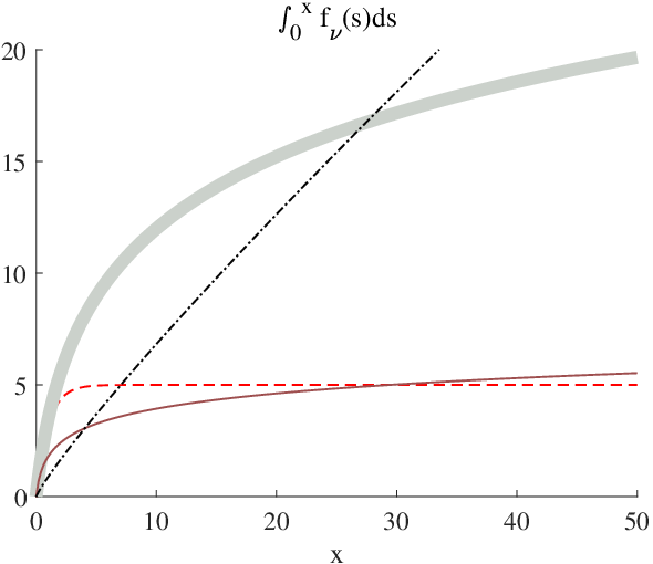
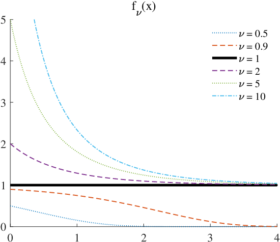
Since and the solutions and will be nonegative. Moreover, if satisfies the Osgood-type condition ( ⋆ ⋆ ⋆ ‣ 1) then the solutions will, for any , remain positive. (The only nonpositive solutions are the trivial solutions starting at .) This plays a role in our main results, as pointed out in the remarks made below Theorem 2.1. In Figures 2 and 3 several solutions of (2.1) are plotted for some choices of .
To proceed we define, for a nondecreasing function and , the domain
| (2.2) |
see Figure 1. Finally, for a subsolution and for we define
and
The following theorem characterizes a sharp lower growth estimate of subsolutions to ( ⋆ ‣ 1) in terms of solutions and to the ODE (2.1):
Theorem 2.1
Using Theorem 2.1 an “explicit” growth estimate can thus be found by estimating the limit as . In Section 3 we will consider certain PDEs for which we can solve the ODE (2.1) explicitly – calculate the limit – and thereby prove Phragmen–Lindelöf type theorems. Let us note that if we can prove
then whenever for some small and thus
Hence, if the integral
converges, then subsolutions may be bounded, but if the integral diverges, then subsolutions must grow to infinity and the conclusion of Theorem 2.1 takes the form of classical Phrgmen–Lindelöf theorems.
We remark that the assumption “ lies on the -axis” is only for notational simplicity; we may translate coordinates otherwise. Note also that Theorem 2.1 holds whenever is replaced (in the theorem and in (2.2)) with , and that Theorem 2.1 gives a growth estimate for any initial condition in (2.1) as long as for some . The best estimate corresponds to the largest . Moreover, it can be realized from the proof of Lemma 2.2 that the assumption “ nonincreasing and nondecreasing” can be replaced by the slightly weaker assumption that is nonincreasing and is nonincreasing ( is nondecreasing) when (). Finally, it will be clear from the proof that we also have for and any . We realize that must increase as long as , which happens whenever satisfies the Osgood-type condition ( ⋆ ⋆ ⋆ ‣ 1). Otherwise, the strong maximum principle does not hold and a positive subsolution to ( ⋆ ‣ 1) may stop growing and attain an interior maximum, see Julin [22] and Lundström-Olofsson-Toivannen [33, Remark 4.3] for a counterexample.
Concerning sharpness of Theorem 2.1 we consider the function
| (2.3) |
vanishing on , depending only on with derivative . In case it holds that and hence we obtain, e.g., that
| (2.4) |
for some function satisfying ( ⋆ ⋆ ⋆ ‣ 1). In case the same holds but with replaced by . Thus, the function defined in (2.3) is a classical solution to an equation of type ( ⋆ ‣ 1) satisfying ( ⋆ ⋆ ‣ 1) and ( ⋆ ⋆ ⋆ ‣ 1). Moreover, it satisfies . In conclusion, when the limit in Theorem 2.1 is positive, the growth estimate cannot be improved, ignoring the shape of and the value of the limit.
Concerning the shape of we note the following. If then independent of , but if then implies that the spherical segment preserves its geometric proportions for all . If is increasing then expands faster in the -direction, implying slightly weaker estimates since , on which supremum is taken, becomes larger. Observe that if the problem is considered in this might be of minor importance, especially if e.g. is bounded in -directions or contained in a cone with apex at the origin. There is not much of a gain to take decreasing since still expands at rate in -directions.
The proof of Theorem 2.1 relies on comparison arguments and the following construction of a classical strict supersolution to ( ⋆ ‣ 1).
Lemma 2.2

Proof of Lemma 2.2. For notational simplicity we set , and . Differentiating yields
It follows that
| (2.5) |
The second derivatives become
for , and
giving
By construction we have and hence
We assume from here on that and decompose so that
Utilizing the structure assumption ( ⋆ ⋆ ‣ 1), the fact that and using (2.5) give
| (2.6) |
since and holds. This last statement follows since by geometry, see Figure 1, and functions are nonincreasing by assumption.
To show that is a strict classical supersolution we need and by (2) and the fact that it suffices to ensure
Observing that holds since is nonincreasing, it suffices to ensure
We know that in so it is enough to have
which holds since we have .
If then by construction and we obtain
| (2.7) |
and thus instead of (2) we end up with
| (2.8) |
Here, the last inequality holds since , is nondecreasing and is nondecreasing in its first argument so that
To ensure that is a strict supersolution we see from (2) that it remains to show that
and we are thus back in the same situation as in the case . The proof of Lemma 2.2 is complete.
Proof of Theorem 2.1. Let be as in the statement of the theorem and denote with the initial condition in (2.1) for which we want to prove the growth estimate. Let and put , where is the strict supersolution in guaranteed by Lemma 2.2.
If on then, if is nonnegative, it follows that and we obtain equality by decreasing . If is nonpositive we note that for some satisfying ( ⋆ ⋆ ⋆ ‣ 1). Thus
which implies that as for all . Therefore, we obtain equality by decreasing also in this case. If on then we increase . If this does not help, (note that we may have , for all and all , for some ), then we lift the supersolution by adding a nonnegative constant. Indeed, for it follows from degenerate ellipticity that also is a strict supersolution. We conclude that
We clarify that if then we have taken . It follows that
and the weak comparison principle in Lemma 1.1 implies that in .
We next conclude that . In particular, assume . By assumption and by the above we have for some , but on the other hand
where the last inequality follows since . Hence, we have a contradiction and we therefore conclude .
Now let , and note that by the comparison principle
Hence is increasing and
| (2.9) |
Inequality (2.9) holds for any independent of . Taking the limit yields
and thus
This completes the proof of the theorem.
3 Applications to well known equations
In this section we apply Theorem 2.1 to some well known PDEs for which we can solve the ODE in (2.1) explicitly – calculate the limit
and conclude explicit growth estimates.
When stating corollaries for specific classes of PDEs we would sometimes prefer to infer other types of “weak” solutions than viscosity solutions whenever such are more suitable or more commonly used for such equations in the literature. As the equivalence of different kinds of ”weak” solutions often is a nontrivial problem we will in some cases avoid going into these details, but this should not make things unclear. The reason is that we only use comparison between “weak” subsolutions and classical strict supersolutions – i.e. Lemma 1.2.
We begin with the simplest case , including e.g. the famous -Laplace equation, proceed with PDEs having sublinear growth in the gradient according to for and end by the variable exponent -Laplace equation, which satisfies assumption ( ⋆ ⋆ ‣ 1) with .
The case
In this simple case the ODE (2.1) reduces to
and hence and . We obtain the limit
| (3.1) |
which is positive if Recalling from the definitions in (2.1) that this forces us to chose the function in the definition of , given by (2.2),
| (3.2) |
Following the remark just below Theorem 2.1 we see that (3.1) implies
| (3.3) |
and we thus retrieve the classical form of the Phragmen–Lindelöf theorem. If the PDE is uniformly elliptic, i.e. , then according to (3.2) we can pick and thereby preserves its geometric proportions for all , which also agrees with the classical Phragmen–Lindelöf theorem. If ellipticity blows up at infinity, i.e. , then the loss in estimate (3.3) comes only in the shape of – it expands faster in -direction since we need to take a larger according to (3.2).
Concerning sharpness of (3.3) we note that with the solution of (2.3) yields
which clearly hits the bottom of (3.3).
Following ( ⋆ ‣ 1) and ( ⋆ ⋆ ‣ 1) we see that (3.3) holds, e.g., for subsolutions of the quasilinear equations
| (3.4) |
corresponding to , where satisfies for all , and
| (3.5) |
whenever is nondecreasing in . One such PDE is the following -Laplace equation, , with lower order terms
| (3.6) |
Indeed, with
where denotes the infinity Laplace operator, we see that satisfies (1.2) with and
whenever . Hence satisfies (1.1) with and and Theorem 2.1 applies.
Recalling that Lemma 1.2 holds for weak solutions (defined in the usual way) to -Laplace type problems or that viscosity solutions and weak solutions are equivalent for some -Laplace type equations , see e.g. Juutinen–Lindqvist–Manfredi [24], Julin–Juutinen [23] and Medina–Ochoa [35], we retrieve the well known Phragmen–Lindelöf results in Lindqvist[29] in the setting of halfspaces.
The case
We now consider equations satisfying ( ⋆ ⋆ ‣ 1) with for some . Note that such satisfies ( ⋆ ⋆ ⋆ ‣ 1) and hence we expect that Theorem 2.1 implies that subsolutions must be increasing on the boundary of . The ODE in (2.1) yields
As is nonincreasing (by assumptions on ) and is nondecreasing we can replace the above equation with the separable ODE
where and . This is possible since solutions of this ODE will approach the origin faster when , and hence it creates a lower bound on the limit in Theorem 2.1. To find the solution for we observe that
and
Thus
and by solving with we also obtain
The limit in Theorem 2.1 becomes, for ,
and for ,
Let’s observe that if which is obtained by taking , then the limits are positive and we obtain
| (3.9) |
Thus, we may derive several Phragmen–Lindelöf type results using Theorem 2.1, whose form will depend on the exponent and the functions , and . For example, using (3)-(3.9) we have proved:
Corollary 3.1
We remark that in Corollary 3.1 we only summarize some examples of growth estimates that take simple forms – the reader may return to conclusion (3.9) for the general case. Note also that all conclusions in Corollary 3.1 are independent of , meaning that we only have to use arbitrary small to prove them. Therefore, since and are nonincreasing functions in this case, we only need that the assumption holds for arbitrary small .
Conclusion takes the form of the classical Phragmen–Lindelöf theorem and when it applies e.g. when
| (3.10) |
, , ellipticity , and . Conclusion holds e.g. when , and . We observe that the exponent in has a borderline value at . Namely, if then subsolutions may be bounded, but if then any subsolution must grow to infinity. As already mentioned in Section 2 such border is, beyond the assumptions in Corollary 3.1, characterized by convergence/divergence of
Conclusion holds e.g. when in (3.10), and .
We further remark that upper bounds on have played an important role for related results in the literature, see e.g. Gilbarg [15], Hopf [19] and Vitolo [40], and that Phragmen–Lindelöf theorems for similar equations in more general domains but with and are proved by Capuzzo-Dolcetta–Vitolo [10] and Koike–Nakagawa [26].
As in the case the results in this subsection apply to PDEs of type (3.4) and (3.5) but now with relaxed assumption on , namely In case of the -Laplace type equation (3.6), , the growth condition on the lower order terms becomes .
When we can explicitly find the classical solution of (2.4), ensuring sharpness, in case of :
Figure 2 shows the solutions for some values of , and different functions .

The case : variable exponent -Laplace equation
We set and obtain the ODE
By the same argument as in the case we replace the above ODE with
where and . This equation separates, when , to
Thus
and since must be nonincreasing this holds for . If the solution takes a similar form. In particular
and
The limit in Theorem 2.1 becomes, for ,
| (3.15) |
which is positive if . Therefore, we have to pick to achieve a growth estimate.
When we know that in (3) stays above 1 if
which forces us to take . Then
as . If the solution decreases to 1 then the limit can be estimated as in (3.15) since follows the expression for with .
In summary, since satisfies ( ⋆ ⋆ ⋆ ‣ 1) we can conclude that for a subsolution satisfying the assumptions in Theorem 2.1 with , the following is true when :
- •
If for some on the -axis and , then may be bounded but
(3.16) - •
If for some on the -axis and , then approaches infinity according to
(3.17)
Thus we retrieve the classical form of a Phragmen–Lindelöf theorem if the subsolution exceeds in (3) with , but if the subsolution only exceeds with , it may grow very slowly and need not approach infinity. The border at originates from the fact that and thus , while for all other positive implying if and if .
The solution of (2.4) with , i.e.
| (3.18) |
ensuring sharpness, can be calculated analytically when and then yields
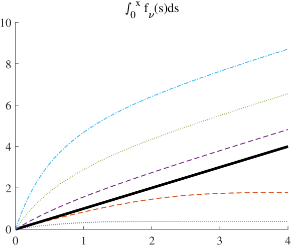
where is the Exponential integral. See Figure 3 (upper row) for some illustrations of the functions in (3) and in (3).
Variable exponent -Laplace equation
The -Laplace equation, which often serves as a model example for PDEs with nonstandard growth, yields
| (3.22) |
The function is usually called a variable exponent. If , then this equation is the classical -Laplace equation and if it’s the famous Laplace equation. Apart from interesting theoretical considerations such equations arise in the applied sciences, for instance in fluid dynamics, see e.g. Diening–Růžička [13], in the study of image processing, see e.g. Chen-Levine-Rao [11] and for electro-rheological fluids, we refer the reader to Harjulehto–Hästö–Lê–Nuortio [17] for a recent survey and further references.
We recall the following standard definition of weak solutions of (3.22): A function is a weak (sub)solution of (3.22) if
for all (nonnegative) . Similarly, is a weak supersolution if is a weak subsolution. A function which is both a weak subsolution and a weak supersolution is called a weak solution. An (USC/LSC) weak (sub/super)solution is called a -(sub/super)harmonic function. We also note that is -harmonic in if it is a local minimizer of the energy
where .
To proceed we define the operator
where denotes the infinity Laplace operator. We note that implies
| (3.23) |
with and . This suggests that -subharmonic functions should be viscosity subsolutions to , which is the case. Indeed, following the proof in Julin [22], which expands on Juutinen–Lukkari–Parviainen [25], we can conclude the following slightly generalized version of [22, Lemma 5.2]:
Lemma 3.2
Suppose that is , , and . If is -subharmonic in a domain , is such that at and then
To obtain a PDE satisfying the required assumptions we redefine by replacing ellipticity with nonincreasing, nondecreasing and also replacing the nonhomogeneous term with , where is nonincreasing in . In particular, we can take
| (3.24) |
In conclusion, a weak USC subsolution (a -subharmonic function) to the variable exponent -Laplace equation is a viscosity subsolution of a PDE of type ( ⋆ ‣ 1) satisfying ( ⋆ ⋆ ‣ 1) and ( ⋆ ⋆ ⋆ ‣ 1). We can therefore conclude that deductions (3.16) and (3.17) hold for -subharmonic functions whenever is and .
We summarize our findings in the following theorem yielding Phragmen–Lindelöf-type results, of which some are sharp, for weak solutions to the variable exponent -Laplace equation:
Theorem 3.3
Suppose that is , , and let be -subharmonic in satisfying
Then is a viscosity subsolution of an equation of type ( ⋆ ‣ 1) satisfying ( ⋆ ⋆ ‣ 1) and ( ⋆ ⋆ ⋆ ‣ 1) with and as in (3). Moreover, if and with from (3) then the following is true:
- •
If somewhere on the -axis for then
- •
If somewhere on the -axis for then
We thus retrieve the classical form of a Phragmen–Lindelöf theorem if the subsolution exceeds with , in particular if it exceeds . On the other hand, if the subsolution only exceeds with , then Theorem 3.3 states that it may grow very slowly and be bounded. The sharpness in the case follows by observing, e.g., that
| (3.25) |
whenever and , for , are constants. It is worth observing that the conclusion
follows also in the case if since then . This holds e.g. if the exponent satisfies and for some constants ; a natural conclusion since these assumptions force the equation toward the constant exponent -Laplace equation far away from the origin.
Versions of Theorem 3.3 are possible to derive from (3.16) and (3.17); e.g., it may be useful to redefine the norm in (3) as . Then, if for all we may divide (3.23) by and conclude, for nonincreasing and nondecreasing, that Theorem 3.3 holds with replaced by and replaced by . In particular, in the case the conclusion then reads
| (3.26) |
We build sharpness of this result in Remark 3.4 below in which we find a family of exponents for which the solution in (3), which satisfies , is -harmonic.
We further remark that Theorem 3.3 sharpens some results of Adamowicz [1] in the geometric setting of halfspaces, and the -assumption on should be replaceable with locally Lipschitz continuity by approximation arguments. Furthermore, the reader may recall the remarks made below deductions (3.16) and (3.17) and also note that contrary to the results in the former subsection, for , the growth estimates here depend on .
Our estimates may not be optimal when is negative since then we lose information by our choice of . We can improve by taking , but we still lose information when subsolutions gradients are not “close to perpendicular” to . This motivates us to derive better estimates under assumptions excluding e.g. the solution in (3.25). We do so by studying a nonpositive ; the case , in the next section.
We proceed by proving the following result, in which we find the “slowest growing” -harmonic function, for a given ellipticity bound, and the corresponding family of exponents.
Remark 3.4
Suppose that and is nonincreasing. Then is the slowest growing -harmonic function in the sense of version (3.26) of Theorem 3.3. In particular, any -subharmonic function with exponent , , and , satisfying
that exceeds somewhere on the -axis satisfies
Finally, if is constant then
where is the Exponential integral.
Proof. Since depends only on and solves (3.18) the first statement follows if we prove that the variable exponent -Laplace equation, with exponent , reduces to the PDE (3.18) in one dimension. Without derivatives in -direction we have
| (3.27) |
Observe that exponent is the unique family of solutions to the ODE
and substituting this equality into (3.27) yields where the “” sign is for when . Thus
which is (3.18) in one dimension.
To prove the second statement we need to ensure that a weak subsolution of the variable exponent -Laplace equation, for some , of which is a solution, is a viscosity subsolution of ( ⋆ ‣ 1) where ( ⋆ ⋆ ‣ 1) holds with the same and as in version (3.26) of Theorem 3.3. To do so we observe that, recalling Lemma 3.2, any -subharmonic function is viscosity solution of
and hence of
Inserting , and assuming that , which we may by taking , we see that
This is a PDE satisfying ( ⋆ ⋆ ‣ 1) with and as in version (3.26) of Theorem 3.3.
It remains to show that satisfies
This holds with equality since
and we have assumed .
The proof is complete.
The case
In this case the ODE (2.1) becomes (we skip the -dependence in only for simplicity)
By the same argument as in the former cases we replace this ODE by
which separates, and we obtain, with
and
The limits become, for ,
and we only need . When we know that in (3) stays above 1 if
which forces us to take . Then
and we need also to achieve a growth estimate.
We have defined in this case. However, from (3) it can be shown that is nondecreasing if . This means that
Now, we let solve this ODE in place of (2.1) and in the proof of Lemma 2.2 we replace (2) with
By tracing the remaining part of the proof of Lemma 2.2 we realize that it is enough to pick .
As in the former situation the solution of (2.4) with can be calculated analytically when :
Now, using the calculations above (3.23) we see that implies
where is the angle between and . Assume and divide the PDE with this factor to obtain
where and for some nonincreasing function and nondecreasing function . Assuming leads to
and we can apply the results from (3)-(3) and Lemma 3.2 to obtain:
Corollary 3.5
Suppose that and are as in Theorem 3.3. Let be the angel between and and assume that
holds in (in a suitable weak sense if is not with ). Then is a subsolution of an equation of type ( ⋆ ‣ 1) satisfying ( ⋆ ⋆ ‣ 1) with , and for some nonincreasing function and nondecreasing function . If and with from (3) then the following is true:
- •
If somewhere on the -axis, then
- •
If somewhere on the -axis, and , then
which, if and is the Exponential integral, implies
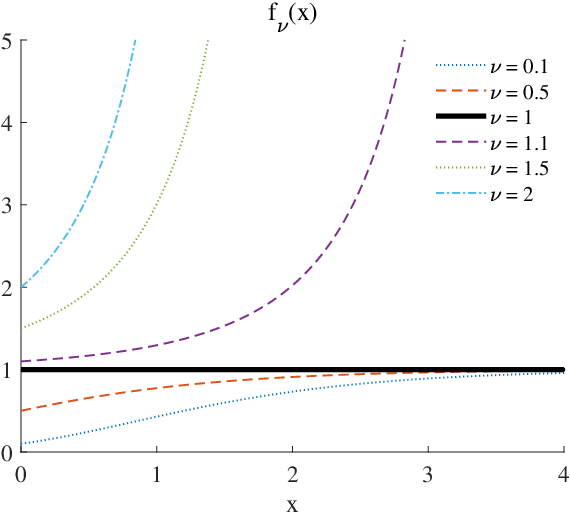
In the one dimensional case Corollary 3.5 shows that if we know that the exponent is increasing, , and that the subsolution satisfies , then , which is much stronger than the growth estimates that can be derived from Theorem 3.3. Similarly, if we know that and then . These improvements can be visualized by comparing the right panels in Figure ; the upper right panel corresponds to Theorem 3.3 while the lower right panel corresponds to the results in Corollary 3.5.
.

.
4 Connections with nonlinear diffusion problems
We follow the presentation in Lundström [31] and let denote the density of some quantity in equilibrium, let be a domain and be a -domain so that the divergence theorem can be applied. Due to the equilibrium, the net flux of through is zero, that is
where denotes the flux density, the normal to and is the surface measure. The divergence theorem gives
Since was arbitrary, we conclude
| (4.1) |
In many situations it is physically reasonable to assume that the flux vector and the gradient are related by a power-law of the form
| (4.2) |
for some factor and exponent , which may depend on space as well. One reason is that flow is usually from regions of higher concentration to regions of lower concentration. From this assumption, with , and from (4.1), we obtain the -Laplace equation
The linear case in (4.2) arises as a physical law in the following: If denotes a chemical concentration, then it is the well known Fick’s law of diffusion, if denotes a temperature, then it is Fourier’s law of heat conduction, if denotes electrostatic potential, it is Ohm’s law of electrical conduction, and if denotes pressure, then it is Darcy’s law of fluid flow through a porous media. A problem involving the nonlinear case is fast/slow diffusion of sandpiles, see Aronsson–Evans–Wu [4]. In that case is very large and models the height of a growing sandpile. If for some , then is very large, and hence the transport of sand is also large, and if , then is very small. Therefore, when adding sand particles to a sandpile, they accumulate as long as the slope of the pile does not exceed one. If the slope exceeds one, then the sand becomes unstable and instantly slides. Other application in which (4.2) arises with is Hele-Shaw flow of power-law fluids (Aronsson–Janfalk [5], Fabricius–Manjate–Wall [14]) and electro-rheological fluids (Harjulehto–Hästö–Lê–Nuortio [17]). When properties of the quantity under investigation depends on space we may model it by a variable exponent in (4.2) and thus enter equations of type (3.22) studied in Section 3.
We will now discuss the problem under investigation from the point of a diffusion problem. Indeed, we will briefly explain, through spatially dependent diffusion, why parts of our results presented in Theorem 3.3 holds true. Suppose that denotes the density of some quantity at equilibrium in the -dimensional halfspace and that (4.2) holds with a variable exponent . Assume also that on the boundary , and at some we assume that . We conclude that then satisfies the -Laplace equation (3.22) in the halfspace and that our results applies. We simplify by further assuming that concentration is independent of -directions. Since must be positive there is a flux of , independent of , flowing perpendicular through the plane at toward the boundary . Due to the equilibrium, the flux must be independent also of and is therefore constant through the halfspace. Since the problem is herefrom independent of , we drop the index and write in the following .


Suppose that is decreasing. As the flux of , given by assumption (4.2), is constant, the concentration must be convex (upwards) if . Indeed, if near the boundary we locally have that (4.2) yields flux and since is decreasing it follows that must be increasing. A similar reasoning explains that if somewhere then the flux implying , and if then must be concave. Figure 4(left) shows examples of how the concentration may depend on for two different decreasing exponents. We remark that if becomes very large near the boundary then must be very close 1 there, otherwise the flux becomes zero or infinity – that is fast/slow diffusion (red solid curve). Similarly, if comes close to 1 as we move into the domain then must grow fast if ever was larger than 1 along the curve in order to keep the flux constant (green dashed curve). Finally, we realize that if becomes constant then becomes constant (recall that is -harmonic when ).
Suppose now instead that is decreasing. Reasoning as in the former case we realize that we may switch our conclusions made near the boundary in the former case with those made further away into the domain. Thus fast/slow diffusion may occur away from the boundary and in such a case the slope of must approach 1. If approaches 1 near the boundary then must explode there, see Figure 4(right).
Returning to (3), (3) and (3.27) in Section 3 we find that the one-dimensional -Laplace equation yields
and with the decreasing exponent
where are a constants, the solution yields
Similarly, with the increasing exponent
the solution yields
With , solution curves for decreasing exponent in (4) are plotted in Figure 3(upper right) (below line ) and (lower right) (above line ),
and solution curves for increasing exponent in (4) are plotted in Figure 3(upper right) (above line ) and (lower right) (below line ).
Compare the structure of these curves to those in Figure 4 with
properties of the exponent in mind.
Acknowledgement. This work was partially supported by the Swedish research council grant 2018-03743.
References
- [1] Adamowicz T. Phragmén-Lindelöf theorems for equations with nonstandard growth, Nonlinear Analysis: Theory, Methods and Applications 97, (2014), 169–184.
- [2] Ahlfors L., On Phragmén-Lindelöf’s principle, Trans. Amer. Math. Soc. 41, (1937), 1–8.
- [3] Armstrong S. N., Sirakov B., Smart C. K. Singular solutions of fully nonlinear elliptic equations and applications. Archive for Rational Mechanics and Analysis, 205(2), (2012), 345–394.
- [4] Aronsson G., Evans L. C., Wu Y. Fast/slow diffusion and growing sandpiles. Journal of Differential Equations, 131 (2), (1996), 304–335.
- [5] Aronsson G., Janfalk U. On Hele-Shaw flow of power-law fluids. European Journal of Applied Mathematics 3.4, (1992) 343–366.
- [6] Avelin B., Julin V. A Carleson type inequality for fully nonlinear elliptic equations with non-Lipschitz drift term. Journal of Functional Analysis 272.8, (2017), 3176–3215.
- [7] Bhattacharya T., On the behaviour of infinity-harmonic functions on some special unbounded domains, Pacific Journal of Mathematics 219, no 2, (2005), 237–253.
- [8] Braga J. E. M., Moreira D. Classification of Nonnegative g-Harmonic Functions in Half-Spaces. Potential Analysis, (2020), 1–19.
- [9] Caffarelli L.A., Cabre X., Fully nonlinear Elliptic equations. American Mathematical Society Colloquium Publications, 43. American Mathematical Society, Providence, RI, 1995.
- [10] Capuzzo-Dolcetta I., Vitolo A., A qualitative Phragmén-Lindelöf theorem for fully nonlinear elliptic equations, J. Differential Equations 243, no 2, (2007), 578–592.
- [11] Chen Y., Levine S., Rao M. Variable exponent, linear growth functionals in image restoration. SIAM J. Appl. Math. 66 (4) (2006), 1383–1406
- [12] Crandall M. G., Ishii H., Lions P.-L. User’s guide to viscosity solutions of second order partial differential equations, Bulletin of the American Mathematical Society, 27 (1992), 1–67.
- [13] Diening L., Růžička M. Strong solutions for generalized Newtonian fluids. J. Math. Fluid Mech. 7 (2005), 413–450
- [14] Fabricius J., Manjate S., Wall P. On pressure-driven hele-shaw flow of power-law fluids preprint 2021.
- [15] Gilbarg D., The Phragmén-Lindelöf theorem for elliptic partial differential equations, J. Rational Mech. Anal. 1, (1952), 411–417.
- [16] Granlund S., Marola N. Phragmén-Lindelöf theorem for infinity harmonic functions, Commun. Pure Appl. Anal. 14 (1), (2016), 127–132.
- [17] Harjulehto P., Hästö P., Lê U. V., Nuortio M. Overview of differential equations with non-standard growth. Nonlinear Analysis: Theory, Methods and Applications, 72(12), (2010), 4551–4574.
- [18] Herzog J. O. Phragmen–Lindelöf Theorems for Second Order Quasi-Linear Elliptic Partial Differential Equations, Proceedings of the American Mathematical Society 15, No. 5, (1964), 721–728.
- [19] Hopf E. Remark on a preceding paper of D. Gilbarg, J. Ration. Mech. Anal. 1, (1952), 419–424
- [20] Horgan C. O., Decay estimates for boundary-value problems in linear and nonlinear continuum mechanics, in: Mathematical Problems in Elasticity, in: Ser. Adv. Math. Appl. Sci., 38, World Sci. Publ, River Edge, NJ, (1996), 47–89.
- [21] Jin Z., Lancaster K., A Phragmén-Lindelöf theorem and the behavior at infinity of solutions of non-hyperbolic equations, Pacific journal of mathematics 211, no 1, (2003), 101–121.
- [22] Julin V. Generalized Harnack inequality for nonhomogeneous elliptic equations. Archive for Rational Mechanics and Analysis 2.216 (2015), 673–702.
- [23] Julin V., Juutinen P. A new proof for the equivalence of weak and viscosity solutions for the p-Laplace equation, Communications in Partial Differential Equations 37.5 (2012), 934–946.
- [24] Juutinen P., Lindqvist P., Manfredi J. J., On the equivalence of viscosity solutions and weak solutions for a quasi-linear equation, SIAM journal on mathematical analysis 33, no 3, (2001), 699–717.
- [25] Juutinen P., Lukkari T., Parviainen M. Equivalence of viscosity and weak solutions for the -Laplacian, Annales de l’Institut Henri Poincare (C) Non Linear Analysis. 27. No. 6. Elsevier Masson, 2010. 1471–1487.
- [26] Koike S., Nakagawa K. Remarks on the Phragmén-Lindelöf theorem for viscosity solutions of fully nonlinear PDEs with unbounded ingredients. Electronic Journal of Differential Equations (EJDE)[electronic only] 2009 (2009): Paper-No.
- [27] Kurta V. V., Phragmén-Lindelöf theorems for second-order quasilinear elliptic equations, (Russian) Ukrain. Mat. Zh. 44, no 10 (1992), 1376–1381; translation in Ukrainian Math. J. 44, no 10 (1992), 1262–1268 (1993).
- [28] M. Leseduarte, M. Carme, R Quintanilla, Phragmén-Lindelöf alternative for the Laplace equation with dynamic boundary conditions Journal of applied analysis and computation 7.4 (2017): 1323–1335.
- [29] Lindqvist P., On the growth of the solutions of the differential equation in -dimensional space, Journal of Differential Equations, 58, (1985), 307–317.
- [30] Lundberg E., Weitsman A. On the growth of solutions to the minimal surface equation over domains containing a halfplane. Calculus of Variations and Partial Differential Equations, 54(4), (2015), 3385–3395.
- [31] Lundström N. L. P., -harmonic functions near the boundary, Doctoral Thesis, ISSN 1102-8300, ISBN 978-91-7459-287-0, Umeå 2011.
- [32] Lundström N. L. P., Phragmén-Lindelöf Theorems and p-harmonic Measures for Sets Near Low-dimensional Hyperplanes, Potential Analysis, 44, (2016), 313–330.
- [33] Lundström N. L. P., Olofsson M., Toivanen O. Strong maximum principle and boundary estimates for nonhomogeneous elliptic equations. arXiv preprint arXiv:2005.03338 (2020).
- [34] Lundström N. L. P., Singh J. Estimates of p-harmonic functions in planar sectors. arXiv preprint arXiv:2111.02721 (2021).
- [35] Medina M., Ochoa P. On viscosity and weak solutions for non-homogeneous p-Laplace equations Advances in Nonlinear Analysis 8 (2017), 468–481.
- [36] Miller K. Extremal barriers on cones with Phragmen–Lindelöf theorems and other applications. Annali di Matematica Pura ed Applicata, 90(1), (1971), 297–329.
- [37] Phragmén E., Lindelöf E., Sur une extension d’un principe classique de l’analyse et sur quelques propriétés des functions monogénes dans le voisinage d’un point singulier, Acta Math. 31, no 1, (1908), 381–406.
- [38] Quintanilla R., Some theorems of Phragmén-Lindelöf type for nonlinear partial differential equations, Publ. Mat 37, (1993), 443–463.
- [39] Serrin J., On the Phragmén-Lindelöf principle for elliptic differential equations, J. Rational Mech. Anal. 3, (1954), 395–413.
- [40] Vitolo A., On the Phragmén-Lindelöf principle for second-order elliptic equations, J. Math. Anal. Appl. 300, no 1, (2004), 244–259.