Quantum Learning Based Nonrandom Superimposed Coding for Secure
Wireless Access in 5G URLLC
Abstract
Secure wireless access in ultra-reliable low-latency communications (URLLC), which is a critical aspect of 5G security, has become increasingly important due to its potential support of grant-free configuration. In grant-free URLLC, precise allocation of different pilot resources to different users that share the same time-frequency resource is essential for the next generation NodeB (gNB) to exactly identify those users under access collision and to maintain precise channel estimation required for reliable data transmission. However, this process easily suffers from attacks on pilots. We in this paper propose a quantum learning based nonrandom superimposed coding method to encode and decode pilots on multidimensional resources, such that the uncertainty of attacks can be learned quickly and eliminated precisely. Particularly, multiuser pilots for uplink access are encoded as distinguishable subcarrier activation patterns (SAPs) and gNB decodes pilots of interest from observed SAPs, a superposition of SAPs from access users, by joint design of attack mode detection and user activity detection though a quantum learning network (QLN). We found that the uncertainty lies in the identification process of codeword digits from the attacker, which can be always modelled as a black-box model, resolved by a quantum learning algorithm and quantum circuit. Novel analytical closed-form expressions of failure probability are derived to characterize the reliability of this URLLC system with short packet transmission. Simulations how that our method can bring ultra-high reliability and low latency despite attacks on pilots.
Index Terms:
5G URLLC, secure access, pilot, quantum learning, superimposed coding.I Introduction
In 5G systems, ultra-reliable low-latency communications (URLLC) has been a basis technology for an entirely new family of mission-critical use cases, such as intelligent transportation, remote healthcare, industrial automation and so forth [1]. As the 3rd Generation Partnership Project (3GPP) claims, URLLC is required to meet the requirements of reliability (99.9999 higher or more) and latency in the order of 1ms or less. To remedy to this, 3GPP has been using a brute-force approach centered on system-level evaluation and a plethora of techniques including short packet transmission [2], grant-free mechanisms [3], leveraging spatial, frequency, and temporal diversity techniques [4, 5, 6]. Among them, grant-free multiple access (GFMA), which deletes the procedures of scheduling request and scheduling grant, has been deemed as a key enabler of URLLC.
In grant-free URLLC, procedures for uplink wireless access have changed significantly with respect to traditional access procedures driven by pre-scheduling [7]. Fig. 1 depicts a general framework of grant-free access procedures under radio resource control (RRC) connected state, including user activity detection (UAD), channel estimation and data transmission. During uplink access, the next generation NodeB (gNB) needs to perform UAD before channel estimation to identify the activities of users that attempt to access URLLC services [8]. However, collision will happen if two or more users that share the same resources perform the uplink access at the same time, and in this case the gNB may not be able to successfully decode all of the uplink transmissions [9]. In view of this, 3GPP specification has regulated the use of pilot-based user identification to distinguish colliding users and the use of pilot-based channel estimation to provide channel information required for decoding data. According to the specification, the gNB needs to allocate different distinguishable pilot resources to different users that share the same resource when collision happens, which means that the process of UAD, channel estimation and data transmission all rely on pilot sequences that are distinguishable from each other.

However, the recent research have shown that pilot-based mechanisms are currently suffering from a high risk of pilot-aware attack, a physical-layer threat that can acquire, jam, spoof and null pilot sequences of interest [10]. Indeed, paralyzing uplink access through tampering with pilots, preferred by attack, is much easier and more efficient than directly disturbing data transmission [11]. When a pilot aware attack occurs in grant-free URLLC, UAD and channel estimation become imprecise, indirectly causing large-scale low-reliability huge-latency data transmission in the uplink. Basically, the above risk stems from the vulnerability that configuration parameters of pilots, including value/frequency location/bandwidth/subcarrier space of pilot sequences, usually decoded from system information before RRC connected, are publicly-known without security protection of upper layer mechanism, like authentication and key agreement, throughout current 5G new radio protocol and easily compromised under pilot aware attack.
Security for 5G URLLC has been studied early by 3GPP System Aspects Working Group 2 (SA2) in [12] and later included in R16 [13], stressing the necessity of security mechanisms to deal with all potential security risks of URLLC on user-plane data transmission. As expected, the protection of pilots in the uplink access has been a critical, complex and unsolved aspect of security for grant-free URLLC. Note that URLLC is for user plane traffic according to TR 23.725 [14] and any upper-layer cryptographic optimization during the very initial registration is not pursued for URLLC services [12]. This imposes novel challenges on the uplink access subject to pilot-aware attack, rooted in the following aspects:
- 1.
Pilot Protection: The maintenance of distinguishability among deterministic pilot sequences is critical but very hard when they are jammed, spoofed and nulled successfully.
- 2.
Complex Access Design: On one hand, the loss of distinguishability among pilot sequences under attack makes both UAD and channel estimation invalid. On the other hand, any scheme trying to protect pilots has to necessarily but toughly support the functionalities of precise UAD and reliable channel estimation.
- 3.
Performance Evaluation in URLLC Scenarios: It is necessary to re-evaluate the influence of uplink access design on reliability and latency performance and to examine whether or not the design satisfy the basic requirements of URLLC services.
I-A Related Works
Recently, it has been pointed out in [15] that 5G URLLC requires a tight coupling between ultra-high reliability and low latency to maintain the same level of security and be efficient in doing so at the same time. The former implies need for stringent security guarantee while the latter implies extremely fast security provision. Progressing towards above goal in uplink grant-free URLLC system needs to tackle lots of open issues, including GFMA, UAD, channel estimation and so forth [15]. These problems, as specified both in standardization and academic communities, revolve around the design of pilot, a critical factor to support precise UAD and channel estimation in grant-free URLLC [9, 16, 17, 18]. In this situation, it is worthwhile to analyze and defend against the threat of pilot aware attack in order to meet the performance requirements for current 5G URLLC. Authors in [19] have investigated the influence of pilot aware attack on GFMA and further stress the importance of pilot protection.
The countermeasures against pilot aware attack have been rarely researched in grant-free URLLC while studied a lot in grant-based systems with non-URLLC services after the seminal work in [20, 21]. The insightful research in this area provide a natural basis for security design in grant-free URLLC system, which can be divided into two main categories, one adopting deterministic-pilot based approach [22, 23, 24] and the other one using random-pilot based approach [25, 26]. The main point of the deterministic-pilot based approach is to insist on storing and using publicly known and deterministic pilots between transceivers. In this case, the attack with strong ability of stealing prior information is quite hard to avoid and the removal of attack is difficult unless discarding the data. What’s more, the countermeasures were limited to solely detecting the existence of pilot-aware attack, rather than further eliminating the attack. Random-pilot based approach was studied to discover security advantages on random signal domain, which provides a potential pathway for recovering true pilots on probabilistic domain. Its security performance was determined by the process of transmission and retrieval of pilot (TRP). Basically, TRP requires that users transmit a set of random pilot sequences from a stored set and then gNB retrieves pilots from the received signals by testing whether or not a pilot sequence of interest is a right member of the stored set.
Initially, the main focus of TRP is on time domain and the design challenge is that random pilot signals transmitted over the air might be completely hidden by random channel taps and attack signals, causing information confusion. Despite the fact that adopting spatial domain property, e.g., natural separation of spatial correlation of massive-antenna arrays, can reduce the effect of attack, the attacker can adjust its correlation property to be similar with one user of interest by roughly revising its spatial location [27]. At this point, the attacker would become more well-directed, rather than less effective.
To address above challenges, many research turn to focus on time-frequency-code domain and encode subcarrier activation pattern (SAP) as robust medium to support TRP [26, 28, 29]. Specifically, subcarriers are activated and encoded as binary non-zero digits when user transmits power on selected subcarriers. Otherwise when user keeps silent on them, those subcarriers are deactivated and deemed as zero digits. Therefore, various SAP candidates can be created and encoded by selectively activating and deactivating subcarriers. In this way, each of pilot signals can be carefully encoded as a unique binary codeword which corresponds to a unique SAP. When pilot signals from all users add up in the air and are received by gNB, the gNB needs to get aware of the subcarrier assignments and inspect the signal power on subcarriers to retrieve the code information. However, random pilot on time-frequency-code domain introduced a novel type of attack-defense domain on which the attack mode observed by gNB is transformed from a pilot-aware attack into a hybrid mode that embraces silence cheating and purely jamming attack [26]. Nevertheless, the feasibility of applying SAP coding method to secure TRP against pilot-aware attack has been verified in [26] in single-user grant-based scenario whereas the scheme can hardly support multiple access.
Actually, the concept of SAP coding has been researched in many literatures in URLLC scenarios. Coding SAP for TRP accords with the URLLC design principle, where exploiting multi-domain diversity has been identified as a promising enabler of URLLC [30]. Furthermore, coding SAP can create a frequency-domain non-square packet structure which has been used as a baseline in 5G new radio since it can minimizes the transmission latency [15]. Authors in [31] have concluded that encoding subcarrier activation patterns (SAPs) to carry information in parallel with data transmission can improve the system reliability with less power and complexity, making it a very suitable candidate for 5G URLLC services. This technique was also studied in grant-free URLLC systems in [32]. However, the coding structure embedded in SAPs cannot directly be employed for pilot protection due to its lack of resilience against attack on code. The design of novel SAP coding method for pilot protection has not attracted sufficient attention in grant-free URLLC.
I-B Motivations and Contributions
The hints above motivate us to design coding principle of SAP for secure uplink access in grant-free URLLC. To this end, we should carefully consider the access procedures under the circumstance of random pilots, random channels and a hybrid attack. SAP coding should be able to protect pilots and at the same time support access procedures. This refers to three basic aspects:
- 1.
Design novel access procedures under SAP coding.
- 2.
Optimize coding principle to resolve the effect of pilot aware attack.
- 3.
Evaluate the reliability and latency performance of novel grant-free URLLC system.
Considering the need for attack defense, we firstly introduce the functionality of attack mode detection (AMD) into uplink access, making access procedures embrace five parts, i.e., AMD, UAD, TRP, channel estimation and data transmission. Indeed, those procedures are expected to highly rely on pilots. Secondly, we exploit the framework of nonrandom superimposed coding on SAPs to protect pilots. In coding theory, the typical nonrandom superimposed code which was first considered by Kautz-Singleton was a set of binary vectors having the property that no vector is contained in a boolean sum (i.e. bitwise OR) of a small number of others [33]. However, the original nonrandom superimposed code cannot provide resilient security attributes. The key task before us is to optimize the code on one hand and make it compatible with new access procedures on the other hand. To achieve the objective, we focus on the joint design of AMD, UAD and TRP through a five-layer quantum learning network (QLN), a precise and computing-efficient solution to the design. Our network not only allows precise AMD and UAD, but also supports quick learning and elimination of decoding uncertainty caused by attack so that TRP can be protected well. The motivation behind QLN is based on the following three key observations: 1) SAP coding brings to the nonrandom superimposed code signal feature which is a useful resource for decoding enhancement but rarely exploited; 2)The decoding uncertainty results from the unauthentic codeword digits generated by SAPs from the attacker. If those digits are found and erased, the attack will be eliminated completely. 3) Quantum learning has the ability of finding the function of uncertainty quickly. The specific goal of QLN is to develop a multi-layer decoding network that can exploit signal features and quantum learning to remove the decoding uncertainty of nonrandom superimposed code under attack. To achieve this goal, the network is required to design AMD and UAD by signal features. Based on this design, the function of identification of unauthentic codeword digits from the attacker can be modelled as a black-box model which is further resolved by quantum parallelism and interference. Key contributions of our work are summarized as follows:
- 1.
Access Design: This work is the first to present a detailed framework of joint design of AMD, UAD, TRP, channel estimation and data transmission under attack on pilots.
- 2.
QLN Design: We show how to use a quantum learning layer to model the identification of unauthentic codeword digits from the attacker during TRP as a black-box boolean function, which is the core of QLN design. Two distinguishable binary quantum states are proved to exist as the inputs of black-box boolean function and the measurement at the output could always get the global information from the two inputs. Thanks to this characteristic, the model can be learned precisely via a quantum circuit and the decoding uncertainty caused by attack can be eliminated completely. In our work, quantum learning is for the first time proved to have the potential of protecting nonrandom superimposed code threatened by attack. Achieving this potential requires the help of signal features. This finding is important for future decoding method design since it provides a framework of modelling and resolving attack uncertainty imposed on information coding.
- 3.
Performance Analysis: Novel analytical closed-form expressions of failure probability of grant-free URLLC system are derived to measure the reliability in the regime of large-scale antenna arrays and short data packets. With these efforts, we can finally show how quantum learning based nonrandom superimposed code can efficiently protect the uplink access in grant-free URLLC.
Organization: In Section II, we review the basic concepts of nonrandom superimposed coding and quantum learning. System model is given in III. Design of QLN for secure uplink access under attack is described in details in Section IV. We also present the design principle of quantum learning layer in Section V and provide the performance analysis in Section VI. Numerical results are presented in Section VII and finally we conclude our work in Section VIII.
II Preliminaries
II-A Nonrandom Superimposed Coding
In coding theory, the situation commonly encountered is that the codewords must be restored from partial information, like defected data (error correcting codes), or some superposition of the strings. These requirements lead to the technique of nonrandom superimposed coding. The typical nonrandom superimposed code which was first considered by Kautz-Singleton is a set of binary vectors having the property that no vector is contained in a boolean sum (i.e. bitwise OR) of a small number of others. Nonrandom superimposed coding has been widely used in various areas, such as, information retrieval for constructing signature files, multi-channel access for wireless communications and so forth.
A nonrandom superimposed code of length and order has three properties:
- 1.
Each codeword has a unique identifier.
- 2.
Each superposition of up to different codewords is unique and each of the superimposed codeword can be correctly decomposed into a unique set of codewords.
- 3.
Each of decomposed codewords from the superimposed codeword is identified uniquely.
With nonrandom superimposed coding, an information transmitter is enabled to express a set of information sequences as discrete codewords. Multiple codewords, when superimposed with each other, e.g., under wireless channel environment or in storage system, can be decoded precisely at receiver according to the pre-shared codebook. Then the receiver tests whether or not a codeword of interest is a right member of the stored set. In order to analyze the coding performance, we consider using the maximum distance separable code [34] to construct the nonrandom superimposed code. The specific construction method can be found in [33]. The rate of superimposed code of length and cardinality , denoted by , is defined by:
| (1) |
where .
II-B Quantum Learning
In quantum information processing, a quantum algorithm is an algorithm which runs on a quantum circuit model of computation [35]. In order to describe the step-by-step computation, it is necessary for any quantum algorithm to develop a suitable quantum oracle, also named as “black-box” oracle. Particularly, if the unknown functions for describing a specific problem is expected to be learned well by quantum algorithms, formulating a precise model of quantum oracle from that problem is the first and most-critical step. There exist lots of quantum algorithms, depending on the specific problems in that application area. One of the first examples of quantum algorithms is Deutsch-Jozsa algorithm which is exponentially faster than any possible deterministic classical algorithm [36]. The algorithm requires two qubits to distinguish constant functions in a black-box problem. A quantum algorithm with single-qubit input is recently proposed to solve the same black-box problem in Deutsch algorithm [37].
Quantum learning is a technique of extracting information from the quantum oracle of quantum algorithm to determine whether or not the oracle has some specific function properties [38]. Typically, such an quantum oracle is assumed to belong to some particular a priori fixed class of possible functions. This model of quantum learning differs from other attempts to use quantum computers to perform machine learning tasks The reason behind the success of quantum learning in this area is the existence of hidden problem structure that quantum computers can exploit in ways that classical computers cannot. Finding such hidden structure in other problems of practical interest remains an important open problem [35]. For example, there is a class of functions that is polynomial time learnable from quantum coherent queries but not from classical queries [39].
In this paper, a concept over is defined by a Boolean function and a concept class is a collection of concepts over . Quantum learning for a concept class is defined as a sequence of unitary transformations ,,,, ,, , where each is a fixed unitary transformation without any dependence on the concept. denotes the quantum membership oracle which is a transformation acting on the computational basis states by mapping where and . Quantum learning provides a quantum state that encodes a hidden function, and its goal is to discover the function efficiently, meaning with a number of queries and an amount of postprocessing that scales polynomially in the number of input bits.

III System Model
III-A System Description of Grant-Free URLLC
We consider an uplink single-input multiple-output (SIMO) orthogonal frequency division multiplexed (OFDM) system with a -antenna gNB (named as Alice) and single-antenna legitimate users (LUs), indexed by the set with . As shown in Fig. 2, this system aims to provide grant-free URLLC services for uplink LUs. We assume that the buffer queues of all LUs are empty after initial system configuration. When new bursty traffic arrives, a total of LUs, indexed by set with , will be activated immediately and then perform GFMA to Alice simultaneously. This is done by transmitting pilot tones and uplink short packet data. For simplicity, we denote those LUs needing bursty traffic transmission as active LUs (ALUs). Correspondingly, Alice is required to perform UAD, channel estimation and uplink data decoding. To this end, traditionally, Alice is supposed to arrange deterministic pilot tones across subcarriers following Block type to support UAD and channel estimation [40]. However, this set-up which is publicly known to all parties inevitably attracts a single-antenna attacker Ava, able to launch a pilot-aware attack (i.e., pilot jamming, spoofing, and nulling attack) on pilot subcarriers to paralyze UAD and channel estimation, further causing data transmission outage. To defend against this attack, Alice and ALUs are required to adopt pilot randomization technique to randomize the values of pilots on each subcarrier. At Alice, three basic functionalities are configured, including
- 1.
AMD: Due to pilot randomization, a novel type of attack-defense domain is introduced on which the attack mode observed by Alice is transformed from a pilot-aware attack into a hybrid mode [26]. The model of attack can be seen in subsection III-D. In such a scenario, AMD which aims to distinguish among different attacks is a critical and necessary functionality.
- 2.
UAD: Rather than relying on deterministic pilots, each ALU has to use random pilot as a temporal identifier to represent itself, compelling Alice to redesign UAD such that the exact number and identities of ALUs can be identified.
- 3.
TRP: As previously talked, the traditional method of TRP cannot hold true under attack. In this paper, pilot signal from each ALU is encoded as a unique SAP. During uplink access, transmission of multiple pilots simultaneously makes SAPs overlap with each other. Alice needs to decode the observed SAPs to retrieve pilots. The model of TRP can be seen in subsection III-C.
It is required for Alice to jointly design AMD, UAD and TRP before channel estimation and data transmission. The relationship among them can be seen Fig. 3. We assume that the joint design of AMD, UAD and TRP occurs on time-frequency resource grid (TFRG)1 defined by a resource block containing subcarriers, OFDM symbols and antennas with . The subcarriers on TFRG 1 are indexed by the set with . For the sake of easy calculation in the following subsections, we define . Channel estimation occurs on TFRG2 defined by a resource block satisfying where the subcarriers on TFRG 2 are indexed by the set with . Data transmission works on TFRG3 defined by a resource block satisfying where the subcarriers on TFRG3 are indexed by the set with . There exist and . and respectively denote the frequency-domain subcarrier spacing and OFDM symbol time, both following the choices in 5G NR numerologies [15]. The total latency during uplink access satisfies the following condition:
| (2) |
where denotes the time occupied by operations other than channel estimation and data transmission. The maximum value of total latency is limited to .
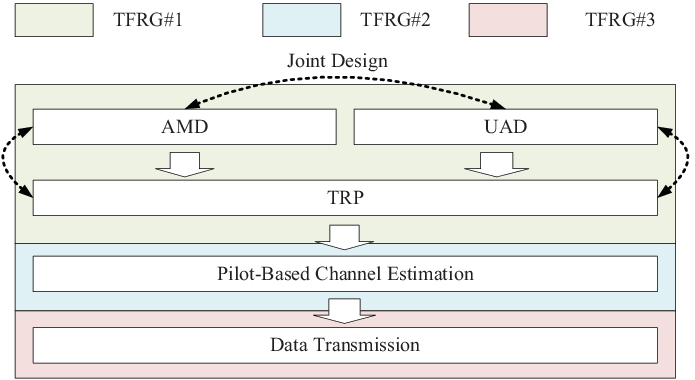
III-B Random Pilot Signal Model
We denote and respectively as the pilot values for the -th ALU and Ava at the -th subcarrier and -th symbol time. satisfies where is a set satisfying . SAP coding for TRP means how to encode as SAPs able to be decoded by Alice, which can be seen in the subsection III-C. Note that can be superimposed onto a dedicated pilot sequence having been optimized under a non-security oriented scenario. The new pilot sequence is then utilized for channel estimation. At this point, is an additional phase difference for security consideration. We do not impose any prior constraints on which satisfies . and respectively denote the transmitting power of pilot signals from the -th ALU and Ava.

III-C Model of TRP
The nonrandom superimposed code of length , size and order for encoding SAPs is denoted by a binary matrix , where each codeword is a column vector. On TFRG1, nonrandom superimposed code based TRP requires that each of codewords in the codebook be mapped as a unique element in set . Besides this, codebook partition and allocation must be done prior to TRP. The codeword vectors in are spilt into independent codeword clusters in which the -th cluster contains codeword vectors indexed by the set . Correspondingly, is equally divided into subsets and we denote the -th subset by . The -th codeword cluster constitutes a sub-matrix denoted by which together with are exclusively allocated to the -th LU.
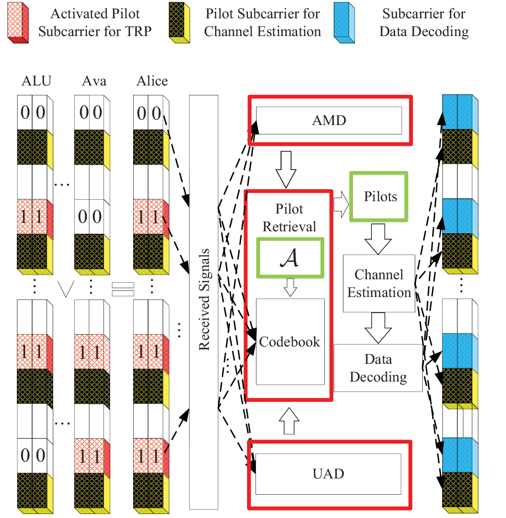
When the -th ALU in the set attempts to use random pilot phase in for TRP at the -th OFDM symbol time, it will select the corresponding codeword in the -th sub-matrix with and further generate its intended SAP according to the codeword . The principle of generating SAPs via is that if the -th digit of is equal to 1, the pilot signal is inserted on the -th subcarrier and otherwise this subcarrier will be idle. According to this principle, ALUs would independently express their pilot phases in the form of SAPs encoded by codewords. This process can be shown in Fig. 4.
Multiple SAPs from different ALUs, after undergoing wireless channels, would suffer from the superposition interference from each other. The codeword superposition is modelled by:
| (3) |
where denotes the boolean sum operation and denotes the codeword exploited by the -th ALU. denotes the codeword from Ava. The specific elements of can be seen in Eq. (4). denotes the superposition version of codewords from ALUs and can be hardly acquired directly by Alice under attack. denotes the codeword that corresponds to the SAP observed by Alice. Note that cannot be derived directly by Alice because what Alice can observe are solely signals on subcarriers. Alice needs to retrieve the information of based on the SAP. As we can see, the above mathematical model represents a complete process of TRP. The framework-level description of AMD, UAD, TRP, channel estimation and data decoding is shown in Fig. 5.
III-D Attack Modelling and Analysis
To destroy the process of pilot retrieval on multiple subcarriers, Ava would launch a hybrid attack mode including:
- 1.
Silence Cheating (SC): Ava keeps silence to misguide Alice since Alice cannot recognize the non-existence of attacks.
- 2.
Wide-Band Pilot (WB-PJ): Ava transmits its random signals on the whole available subcarriers to cover the codeword information of all ALUs.
- 3.
Partial-Band Pilot Jamming (PB-PJ): Ava transmits its random signals on arbitrary part of the whole subcarriers such that the codeword decoded by Alice is imprecise.
Under above model, the elements of vector , determined by attack modes, can be given by:
| (4) |
Note that Ava does not know the codeword used by ALU of interest since codewords from ALUs are randomly selected. Furthermore, the distribution of above attack modes is unknown to Alice and LUs. Therefore, the coding principle of SAP at Ava is to use random coding on SAPs. By examining Eq. (3) and Eq. (4), we can easily test the ability of nonrandom superimposed code in resisting attack. For example, let us consider three codewords from ALUs, i.e., , , and a codeword from Ava, i.e., . Since signal energy from Ava is dispersed on pilot subcarriers, what Alice could observe is a WB-PJ attack, which indicates no any useful information and imposes huge confusion on SAP decoding.
III-E Pilot Based Channel Estimation
Consider the basic OFDM procedure on TFRG2. Pilot tone vectors of ALUs and Ava over subcarriers are respectively stacked as by 1 vector and . We consider using orthogonal pilots, i.e., . The length of cyclic prefix is assumed to be larger than the maximum number of channel taps. The parallel streams, i.e., and are modulated with inverse fast Fourier transform. Then the time-domain by 1 vector , derived by Alice after removing the cyclic prefix at the -th receiving antenna, can be written as:
| (5) |
Here, is the circulant matrices of the -th ALU, with the first column given by . is a circulant matrix with the first column given by and is assumed to be independent with . and denote the channel impulse response vectors, respectively from the -th ALU and Ava to the -th receiving antenna of Alice. denotes the length of channel taps. denotes the discrete Fourier transform matrix. denotes the noise vector on time domain at the -th antenna of Alice within the -th symbol time. is the average noise power of Alice. Taking fast Fourier transform, Alice finally derives the frequency-domain by 1 signal vector at the -th receiving antenna as:
| (6) |
where . denotes the first columns of . satisfies:
| (7) |
where . Stacking within OFDM symbol time, we can rewrite signal model in Eq. (6) as:
| (8) |
where the matrix satisfies and satisfies . The vector satisfies .
Provided that TRP can be protected well, the random pilot of interest, i.e., -th one, can be known by Alice without being affected by Ava. A least square estimation of , denoted by can be given by:
| (9) |
where is the Moore-Penrose pseudoinverse.
| (13) |
III-F Data Transmission
Without loss of generality, we assume: 1) ALUs share the same subcarriers at the same OFDM symbols within TFRG3 for short packet transmission; 2) ALUs operate at the same rate which can be calculated as ; 3) Alice employs matched filter over antennas on each subcarrier. Under above assumptions, the receiving signal model of Alice at the -th subcarrier within the -th OFDM symbol is denoted by , satisfying
| (10) |
where denotes the data symbol transmitted by the -th ALU at the -th OFDM symbol and satisfies where is the instantaneous signal-to-noise-ratio (SNR). denotes the noise vector at the -th subcarrier within -th OFDM symbol and satisfies . denotes the -th subcarrier channel vector stacked by the -th ALU across antennas, and satisfies:
| (11) |
where denotes the -th row of . We define as the estimated version of and can derive the estimated version of as , satisfying:
| (12) |
Based on , Alice derives the matched filter as which is then applied on Eq. (10) to decode the data symbol of -th ALU. Receiving signal weighted by can be expressed in Eq. (13). We assume when no estimation errors exist, and otherwise we assume where is independent with and larger means that the estimation gets worse.
IV QLN for Secure Uplink Access Under Attack
In this section, we concentrate on the joint design of AMD, UAD and TRP through a five-layer QLN. The QLN includes a initial layer, input layer, hidden layer, quantum learning layer and output layer. Details on the design of each layer are given in Fig. 6 and discussed in the following subsections.
The design principle of layers in QLN depends on the processing procedures for decoding SAP. Since what Alice can directly observe are solely signals on subcarriers that follow an unexpected SAP, decoding the SAP needs to achieve a signal-feature based transformation from signals to binary code information, a complex and multi-step process following a fixed order. Hence it is natural to adopt multiple layers, each layer responsible for one specific functionality. QLN uses different layers to abstract increasingly complex procedures, i.e., an initial layer is to model signal information, an input layer to extract signal feature, an hidden layer to deal with features etc. This often leads to better generalization ability towards future access design in 5G and Beyond. Besides, this set-up can help gNB easily learn more detailed functionalities within each layer and more abstract relationships among different layers. It is theoretically possible to represent any possible functionalities with a single layer QLN. In order to achieve single layer QLN, it is required to change the method of SAP coding correspondingly, which could be a future research direction. Universal approximation which states that the least layer required to approximate any SAP decoding procedures can be also researched in the future. In this paper, we will provide an easy-to-implement and initial version of QLN, for the sake of making clear the basic design principle in this area.

IV-A Initial Layer
The functionality of initial layer is to provide data information required by the network and to give a mathematical model describing those data well. This layer is constituted by initial nodes among which initial nodes are responsible for collecting and modelling wireless signals on resource block and another node stores all the available codebook matrices related to the nonrandom superimposed code.
IV-A1 Data on the First Initial Nodes
The encoding principle of SAPs determines that subcarriers are expected to be randomly occupied by random pilot signals. When ALUs attempt to access, we define the possible number of signals on the -th subcarrier as . Then the signals within the -th OFDM symbol on the -th initial node of this layer can be denoted by , satisfying:
| (14) |
where denotes the channel vector from Ava to Alice at the -th pilot subcarrier across antennas, and satisfies:
| (15) |
denotes the interfering signal from Ava at the -th pilot subcarrier within the -th OFDM symbol.
Let us explain the Eq. (14) in details. holds true when no pilot signals arrive; If interfering signals from Eva are received by Alice, there will be ; Otherwise if pilot signals from ALUs arrive at Alice, holds true; Finally, if signals from both ALUs and Eva coexist, there will be .
By stacking signals across OFDM symbols at the -th pilot subcarrier, Alice derives the data captured by the -th initial node as a matrix , given by:
| (16) |
where the parameter is unknown now and will be given in the following section, depending on specific design requirements.
IV-A2 Data on the -th Initial Node
We define the matrix as the collection of all of the boolean sums of codewords from , taken exactly at a time. Each column vector of represents a unique codeword. The -th node is responsible for storing the stacked matrix of superimposed code, denoted by , satisfying:
| (17) |
As we can see, the final outputs of initial layer are and .
IV-B Input Layer
The input layer is responsible for signal feature extraction which provides quantized signal features necessary to SAP decoding. Three types of nodes for achieving this functionality are prepared, including energy feature extraction (EFE) nodes, independence feature extraction (IFE) nodes and code storage (CS) node.
IV-B1 EFE Nodes
There exist a total of EFE nodes, each node performing signal energy detection on the corresponding subcarrier so as to accurately determine the number of signals on the subcarrier.
In order to perform signal energy detection on the -th pilot subcarrier, Alice needs to make the -th EFE node generate a normalized covariance matrix that satisfies . The ordered eigenvalues of are given by . After that, Alice constructs test statistics as where denotes the decision threshold of the -th test statistic. The hypothesis means signals coexist and means the opposite. If Alice hopes to recognize signals precisely, both and should hold true. Otherwise if Alice hopes to recognize signals, should hold true. Based on eigenvalues, Alice cannot recognize signals. In fact, Alice needs to detect at most signals including signals from ALUs and one signal from Ava on each subcarrier. This requires such that the eigenvalue space of is enough to capture features of all possible signals.
For , the larger is, the larger threshold is required to make precise decision. To detect all possible signals without false alarm, is utilized as the common threshold for all other detectors, i.e., . Given , Eq. (49) in [41] provides a threshold function to measure what level the probability of false alarm, i. e., , can achieve. We should note that this function is not only a monotone decreasing function of but also a monotone increasing function of . For a given probability constraint , a lower bound could be always expected with . Under this equation, zero can be achieved by flexibly configuring and can be determined exactly [41]. This phenomenon can be experimentally confirmed in Fig. 7 where is fixed to be and is respectively configured as 12, 16, and 20. Basically, this phenomenon originates from the well-known Marcenko-Pastur Law [42]. In this paper, we let .
Based on above method for establishing the decision threshold, Alice constructs test statistics as . After testing above statistics, Alice can derive the number of signals at the -th subcarrier as . Finally, we rewrite the function of this EFE node as a function with the output , satisfying:
| (18) |
IV-B2 IFE Nodes
There are a total of IFE nodes and each IFE node performs inner-product operation across all subcarriers so as to accurately capture the independence features embedded in pilot signals from ALUs and Ava.
Our treatment of independence characteristic of receiving signals will refer to two aspects, that is, wireless channels and random pilot signals. Particularly, it is well known that wireless channels from different ALUs are independent with each other due to the inherent constraints of antenna spacing. Thanks to the transparency transmission set-up in the uplink in current 3GPP specification, pilot signals from different ALUs are also independent with each other.
In order to quantize above independence features having embedded on the pilot subcarriers, IFE nodes need to perform the mutual inner-product operation among pilot signals at different frequency-domain positions. The inner-product operation between pilot signals at the -th pilot subcarrier and those at the -th pilot subcarrier can be derived as:
| (19) |
where denotes the differential code digit and denotes inner product operation. represents the encoder satisfying where denotes the decision threshold. The value of at the -th pilot subcarrier can be seen in Eq. (14). To identify the principle of designing , we give the following interpretation. According to law of large numbers, the inner product between signals from two independent individuals approaches zero. On the contrary, the inner product between signals from the same node can reach a value with its amplitude equal to one. In theory, the value of can thus be configured to be a certain value, i.e., 0.5.
On this basis, the independence features having embedded on the -th pilot subcarrier can be extracted as the binary code vector . See more details about the extraction process in Algorithm 1. Based on above algorithm, we define the function of the -th IFE node as , satisfying:
| (20) |
where and respectively denote the input and output of the -th IFE node.
IV-B3 CS Node
CS node is responsible for storing the data from the -th initial node. We define the function of this node as function , satisfying
| (21) |

IV-C Hidden Layer
This layer is responsible for dealing with those quantized features having been derived in the previous layer. This is done through three types of nodes, i.e., energy feature processing (EFP) node, independence feature processing (IFP) nodes and CS node.
The function of EFP node, denoted by , is to encode the detected number of signals on subcarriers and output a multivariate codeword vector , given by:
| (22) |
where
| (23) |
and
| (24) |
where is the indicator function.
The IFP nodes have two functionalities. For the first functionality, IFP nodes generate according to the Eq. (24) and then make the -digit of zero to derive a codeword denoted by . The overall functionality is denoted by a function , satisfying
| (25) |
The second functionality is to stack as a matrix satisfying . This task is accomplished by another IFP node and can be described by a function , satisfying:
| (26) |
The functionality of CS node in this layer is the same as that in the input layer.
IV-D Quantum Learning Layer
As we mentioned previously, the core of joint design of AMD, UAD and TRP lies in how to find the unauthentic codeword digits generated by SAPs from the attacker. This is done by the quantum learning layer. To this end, this layer firstly configures a detection node to realize AMD and then configures identification nodes to learn the attacker’s codeword digits. CS node is also configured to provide the matrix .
IV-D1 AMD
The functionality of AMD at detection node is built on the following three principles: (1) WB-PJ attack happens only when is a all-ones matrix, (2) PB-PJ attack happens when or , , (3) SC happens when and . Following above principles, the function of detection node, denoted by , satisfies:
| (27) |
where when and otherwise .
IV-D2 Identification of Codeword Digits from Ava
Let us define to indicate whether the pilot signal on the -th subcarrier is from Ava or not. When is equal to 1, Alice can determine that the pilot signal on the -th subcarrier is transmitted by Ava. Based on this principle, we can know that holds true when Alice identifies WB-PJ attack successfully since the codeword of Ava in this case is a vector of all ones. Provided that SC attack is identified successfully, Alice can know that would be a zero vector and holds true. When PB-PJ attack is identified, the situation is rather complex, discussed as follows:
If , there exist two possibilities including and . For these two cases, Alice can precisely know which ALU is currently being interfered by Ava. This is done by checking to examine whether is a vector in or not. If the -th one is, the is deemed to be the codewords of Ava and configures .
If , there exists . The discussion is divided into two aspects: 1) can be included by . In this case, there will be and Alice can perfectly identify codewords from ALUs even though is unknown. For simplicity, we define as a zero vector; 2) cannot be not included by . In this case, there must exist and a set satisfying . Alice needs to calculate and examine whether is a vector in or not. If it is, the value of is stored in the set with , and Alice configures . In this way, Alice can always recognize as .

Based on above decoding principle, we model the function of the -th identification node on this layer as a function satisfying:
| (28) |
where the choices of values of can be 0 and 1, depending on the specific design. More specifically, when configuring , Alice examines whether there exists by checking in codebook . This process is defined as decision function which outputs 0 if and otherwise 1. Otherwise when , Alice has two options, respectively represented by two subfunctions, i.e., if and if . The details can be shown as follows:
- 1.
is a decision function. Firstly, it configures the -th digit of to be zero and derives the revised codeword. Then it outputs 0 if this revised codeword belongs to and otherwise 1.
- 2.
is a decision function which outputs 1 if and otherwise 0.
As we can see, the above function describes the decoding principle well. For the sake of convenience, in what follows, we denote by .
IV-E Output Layer
Based on the output of previous layer, this layer aims to perform UAD and to eliminate the effect of codeword digits from Ava such that those codewords from ALUs can be recovered. Apart from the CS node, this layer contains two new nodes, one defined by the UAD node and the other one defined by decoding node. The function of UAD node and decoding node can be respectively modelled as and , respectively satisfying:
| (29) |
and
| (30) |
The details of above two functions are given as follows. When WB-PJ attack has been identified in quantum learning layer, i.e., , is updated as , . Correspondingly, Alice encodes the number of signals on each subcarrier and derives the novel codeword which satisfies . could be derived by decomposing based on the codebook matrix . If SC attack has been identified, i.e., , could be derived directly since . The above two cases mean that the number and identities of ALUs, together with their codewords, can be precisely determined under WB-PJ and SC attack. Otherwise when PB-PJ attack has been successfully identified in quantum learning layer, i.e., for , Alice changes the -th code digit of to be zero. Based on the decoding principle of nonrandom binary superimposed code, Alice can derive a new binary codeword enabled to be decomposed as . Using this method, Alice can know the number and identities of ALUs and their codewords precisely under PB-PJ attack. We can say that UAD can be performed precisely along with the codeword decoding.
V Design Principle of Quantum Learning Layer
In this section, we focus on the function in quantum learning layer and reveal its intrinsic potential for the support of quantum learning to capture the uncertainty of codewords from Ava.


V-A The Property of Function
Based on the decoding principle discussed in the previous layer, we can show the structure of in Fig. 8. Since and are random, , and are basically random binary digits. Note that the values of are also binary digits. Therefore, we can have the following proposition.
Proposition 1.
is a black-box boolean function which aims to compute the following function:
| (31) |
Theorem 1.
If is a balanced function, the -th codeword digit belongs to ALU. Otherwise when is a constant function, the -th codeword digit belongs to Ava.
Proof.
In principle, a boolean function can be either a constant function or a balanced function. In order to determine whether the -th digit belongs to Ava, Alice has to calculate the function . If , the boolean function is balanced and Alice confirms that the -th codeword digit belongs to Ava undoubtedly. Otherwise if , the boolean function is constant and the -th codeword digit belongs to ALUs. ∎
The problem of identifying codeword digits from Ava has been transformed into an issue of how to compute the black-box boolean function .

V-B Quantum Learning Algorithm
We in this subsection explore quantum membership oracle to support quantum learning to learn whether the function is constant or balanced. A quantum membership oracle is a unitary transformation that acts on the computational basis states as:
| (32) |
where denotes a quantum circuit for on the second qubit, shown in Fig. 9. denotes the first input qubit while denotes the second one. When the second input qubit is configured to be in the state , then in the first input qubit will give in the second output bit. Similarly, in the first input qubit will give . Therefore, can be deemed as a quantum version of the (classical) input bit 0, and as a quantum version of the input bit 1. If the quantum circuit is expected to resolve a specific classical problem, the input and output should be designed deliberately.
Now let us turn to the design of quantum circuit. We define the first qubit as control qubit and the second qubit as target register. For the control qubit, two Hadamard gates are configured, respectively at the input and output. This can be seen in Fig. 10. Besides, we configure a G gate at the input of target register. The input before the G gate is from the control qubit. The G gate is defined by . We also configure a P gate which is expressed as at the second output.
In what follows, we specify the working principle of quantum circuit using four 2-qubit basis vectors, i.e., , , and . Note that , and are just the imitate representation of quantum state for the sake of our understanding, rather than the results in measurement, since each measurement will change the quantum state. Those bases can be expressed by:
| (33) |
| (34) |
| (35) | |||||
Examining Eq. (35), we know that when , the result holds true. The final Hadamard gate on the control qubit and and P gate on the target register transform the state to:
| (36) |
As we can see, we need to solely focus on the measurement of control qubit. Obviously, the squared norm of the basis state in the control qubit is 1, meaning that when one measurement of the control qubit is certain to return the value 0. Similarly, when one measurement of the control qubit is certain to return the value 1. One measurement of the control qubit can directly determine the value of . Therefore, Alice using above quantum circuit can decide whether or not the codeword digit at belongs to Ava at the cost of only half of the query complexity of original nonrandom superimposed coding.
In our design scheme, a quantum circuit with a single qubit is sufficient to implement an quantum oracle. Note that the scheme in [37] also proposed an example for quantum computation task with a single-qubit input. However, it requires at least a three-level quantum system and has special requirements on the computational task, i.e., determining parity of cyclic permutations. Different from that, our scheme is independent with the computational task even for a two-level quantum system, which can be well generalized to higher dimensional cases.
Finally, we provide the overall implementation details of QLN in decoding process of nonrandom superimposed code on SAPs in Fig. 11.
VI Performance Analysis
In the previous sections, we have detailed the principle of joint design of AMD, UAD and TRP in QLN, and also shown how to eliminate the effect of pilot-aware attack completely. Benefiting from this, the new grant-free URLLC system under pilot-aware attack can maintain normal channel estimation and data decoding by consuming OFDM symbols and pilot subcarriers. However, we still need to analyze the reliability performance of this grant-free URLLC system. To this end, we consider using the channel estimation model shown in Eq. (9) and the data transmission model shown in Eq. (13). The goal is to derive the expressions of failure probability for the grant-free URLLC system.
Basically, a certain probability of failure occurs in uplink short packet data transmission due to the inevitable decoding error of short packets. There has been a well-known expression in literature [43] to calculate the decoding error probability of transmissions over fading channels as a function of the average received SNR , the transmission rate and matched filter receiver, given by:
| (37) |
where , and . On each subcarrier within TFRG3, interfering signals coexist and there exists . Without loss of generality, we assume interfering signals are Gaussian distributed and received at Alice with the same average SNR . The distribution under matched filter receiver satisfies:
| (38) |
where denotes the Gamma function.
In this paper, we assume at most one retransmission can be supported in the uplink. Since TRP and UAD are both precise, the first transmission is deemed successful if its data is decoded successfully. In this case, the probability of correct data decoding is . Otherwise, the ALU would perform a retransmission over shared resources. The probability of correctly decoding the retransmitted data can be calculated by . Finally the failure probability of grant-free URLLC system, denoted by , is given by:
| (39) |
Theorem 2.
With precise CSI estimated, the asymptotic expression of received signal-to-interference-plus- noise ratio (SINR) at Alice as is given by:
| (40) |
and the result with estimation error is given by:
| (41) |
The decoding error probability satisfies:
| (42) |
and the failure probability of grant-free URLLC can be finally expressed as Eq. (43). The specific value of depends on the estimation assumption above.
| (43) |
Proof.
Eq. (13) represents the model of received signal from the -th ALU. According to the strong law of large numbers [42], the following equations hold true
| (44) |
| (45) |
| (46) |
When , the received SINR for the -th ALU can be written as:
| (47) |
Eq. (40) can be derived after simplification. The received SINR for the -th ALU under estimation errors can be written as:
| (48) |
where . After simplification, we can derive the Eq. (41). Due to the disappearance of channel randomness under large number of antennas, we can calculate Eq. (37) as Eq. (42). By substituting Eq. (42) into Eq. (39), we can derive Eq. (43). The proof is complete. ∎
VII Numerical Results
| Simulation Parameters | Values |
| Modulation | OFDM |
| Subcarrier spacing | 60kHz,120kHz |
| Channel bandwidth | 100MHz, 400MHz |
| Coherence bandwidth | |
| OFDM symbol duration | |
| Number of OFDM symbols for TRP | |
| Number of subcarriers for TRP | |
| Number of subcarriers for channel estimation | |
| Pilot subcarrier arrangement for TRP | Proposed Coding |
| Pilot subcarrier arrangement for channel estimation | Block type |
| Channel estimator at gNB | Least Square |
| Number of subcarriers for data transmission | |
| Combing technique at gNB | Matched filter receiver |
| Size of data packets | |
| SINR of receiving data at gNB | |
| Time consumed by other operations | |
| Number of antennas at gNB | |
| Channel fading model | Rayleigh |
| Number of ALUs | |
| Number of channel taps | |
| Failure probability requirement | |
| Latency constraints |
In this section, we will evaluate the performance of uplink access of grant-free URLLC using quantum learning based nonrandom superimposed coding, This refers to several metrics, including the code rate, overheads, reliability and latency under channel estimation errors. Frequency range 1 (FR1) for Sub-6 GHz and Frequency range 2 (FR2) for millimeter wave in 5G NR are considered respectively. The system is expected to work within at most 100 MHz channel bandwidth for FR1 and at most 400 MHz channel bandwidth for FR2 [44]. Simulation parameters and values can be seen in Table I. Note that one pilot every three consecutive subcarriers is inserted to acquire independent frequency-domain variations of the channels. Given above bandwidth constraints, the maximum number of pilot subcarriers for TRP is limited to 512. Therefore, at most channel bandwidth is occupied when and at most channel bandwidth is required when .

Fig. 12 presents the curve of code rate versus . As we can see, increasing and will reduce the code rate; for example, decreases from 0.06 to 0.05 if increases from 4 to 8 at and . Furthermore, increasing will increase the code rate; for example, increases from 0.07 to 0.085 if increases from 2 to 3 when and ; Increasing will also increase since the lower bound of available , that is, , increases with the increase of ; for example, when , the increase of from 8 to 12 will increase the lower bound of from 72 to 156. We can also find that the influence of proposed scheme on frequency-domain resource overheads is greater than that on code-domain resource overheads, which means that higher degree of optimization on code rate can be performed to reduce the subcarrier resource consumption, given a certain level of reliability.

In order to clearly investigate the influence of the proposed scheme on time-frequency resource overheads, we in Fig. 13 present the curves of versus , respectively under and . The parameter satisfies . is fixed to be and is configured under . When increases from 4 to 12, the total latency and the subcarrier overheads both increase. This tendency does not change under various , meaning that both time-domain and frequency-domain resources are critically important for pilot protection. Indeed, pilot subcarriers under are consumed more with respect to those under . This is because larger can bring higher coding diversity on code domain and thus reduce the consumption of frequency-domain resources. Fig. 13 also verifies the fact that the influence of proposed scheme on frequency-domain resource overheads is greater than that on time-domain resource overheads.

Fig. 14 shows the curves of failure probability versus channel estimation error . with and with are respectively configured under and . is determined by with . As we can see, increases with the increase of if is above a certain threshold which changes with the number of ALUs. When increases, the fluctuation of this threshold is more sensitive to the changes of channel estimation errors. Since channel estimation errors cannot be eliminated completely, more ALUs would introduce more intra-user interference and disturbance caused by imprecise channel estimation. Especially when is configured to be larger than 16, FR1 cannot support proposed new grant-free URLLC system.

Fig. 15 depicts the reliability-latency tradeoff curves under various . is configured to be 128 and is selected from to . is fixed to be and is configured to be under . is chosen as . We can see that data transmission latency should not be lower than a certain threshold if it is expected to achieve the reliability of or more. With the increase of , the failure probability is increased and the reliability is decreased. Especially when is equal to 32, the system reliability can hardly satisfy the requirements of 5G URLLC. Those hints provides guiding principles for designing and implementing grant-free URLLC system under pilot-aware attack.
VIII Conclusions
In this paper, we proposed a quantum learning based nonrandom superimposed coding method to support flexible, secure and efficient SAP encoding/decoding such that those SAPs can be used for TRP in uplink access process of grant-free URLLC systems threated by a pilot-aware attack. This design changed the main access procedures as those including AMD, UAD, TRP, channel estimation and data transmission. A quantum learning network was designed to learn the uncertainty of attack on SAP decoding precisely. With the help of this network, AMD, UAD and TRP could be precisely realized and meanwhile the performance of channel estimation and data transmission can be recovered to a normal level. By considering those procedures together, we derived novel expressions of failure probability of the new grant-free URLLC system to evaluate its reliability. With above efforts, we can say that it is feasible to use quantum learning to help information coding defend against unknown attack on itself, which is an interesting direction for future research.
References
- [1] 3GPP, TS22.261 v16.1.0,“Servic requirements for the 5G system,” [online]Available: https://www.3gpp.org/ftp/specs/archive/22series/22.261
- [2] G. Durisi, T. Koch, and P. Popovski, “Toward massive, ultra-reliable, and low-latency wireless communication with short packets,” Proc. IEEE, vol. 104, no. 9, pp. 1711–1726, Sep. 2016.
- [3] R1-1703329, “UL grant-free transmission for URLLC,” Feb. 2017.
- [4] M. Bennis, M. Debbah, and V. Poor, “Ultra-reliable and lowlatency wireless communication: Tail, risk and scale,” Proc. IEEE, vol. 106, no. 10, pp. 1834–1853, Oct. 2018.
- [5] A. Mahmood et al., “Time synchronization in 5G wireless edge: Requirements and solutions for critical-MTC,” IEEE Commun. Mag., vol. 57, no. 12, pp. 45–51, Dec. 2019.
- [6] 3GPP,TR38.824, v16.0.0,“Study on physical layer enhancements for NR ultra-reliable and low latency case (URLLC),” [online]Available: https://www.3gpp.org/ftp/Specs/archive/38series/38.824
- [7] K. S. Kim et al., “Ultrareliable and low-latency communication techniques for tactile Internet services,” Proc. IEEE, vol. 107, no. 2, pp. 376–393, Feb. 2019.
- [8] L. Liu and W. Yu, “Massive connectivity with massive MIMO-Part I: Device activity detection and channel estimation,” IEEE Trans. Signal Process., vol. 66, no. 11, pp. 2933-2946, Jun. 2018.
- [9] 3GPP TR 36.881 v14.0.0, “Study on latency reduction techniques for LTE,” [online]Available: https://www.3gpp.org/ftp/Specs/archive/36 series/36.881
- [10] C. Shahriar, M. La Pan, M. Lichtman, T. C. Clancy, R. McGwier, R. Tandon, S. Sodagari, and J. H. Reed, “PHY-Layer resiliency in OFDM communications: A tutorial,” IEEE Commun.Surveys Tuts., vol. 17, no. 1, pp. 292-314, Aug. 2015.
- [11] T. C. Clancy and N.Georgen, “Security in cognitive radio networks: threats and mitigations,” in Proc. 3rd Int. Conf. CrownCom., May 2008, pp. 1-8.
- [12] 3GPP TR 33.825 v16.0.1, “Study on the security of Ultra-Reliable Low-Latency Communication (URLLC) for the 5G System (5GS),” [online]Available: https://www.3gpp.org/ftp/Specs/archive/33series/33.825
- [13] 3GPP TS 33.501 v16.3.0, “Security architecture and procedures for 5G system,” [online]Available: https://www.3gpp.org/ftp/Specs/archive/33 series/33.501
- [14] 3GPP TR 23.725 v16.2.0, “Study on enhancement of Ultra-Reliable Low-Latency Communication (URLLC) support in the 5G Core network (5GC),” [online]Available: https://www.3gpp.org/ftp/Specs/archive/23 series/23.725
- [15] H.Ji, S. Park, J. Yeo, Y. Kim, J. Lee, and B. Shim , “Ultra-reliabie and low-latency communications in 5g downlink: Physical layer aspects,” IEEE Wireless Commun., vol. 25, no. 3, pp. 124-130, Jun. 2018.
- [16] T. Jiang, Y. Shi, J. Zhang, and K. Letaief, “Joint activity detection and channel estimation for IoT networks: Phase transition and computationestimation tradeoff,” IEEE Internet Things J., vol. 6, no. 4, pp. 6212-6225, Aug. 2019.
- [17] Z. Chen, F. Sohrabi, and W. Yu, “Sparse activity detection for massive connectivity,” IEEE Trans. Signal Process., vol. 66, no. 7, pp. 1890-1904, Apr. 2018.
- [18] Y. Li, M. Xia, and Y.-C. Wu, “Activity detection for massive connectivity under frequency offsets via first-order algorithms,” IEEE Trans. Wireless Commun., vol. 18, no. 3, pp. 1988–2002, Mar. 2019.
- [19] Q. Qi, X. Chen, C. Zhong, and Z. Zhang, “Physical layer security for massive access in cellular internet of things,” Sci. China Inf. Sci., vol. 63, no. 2, pp. 1-12, 2020.
- [20] T. C. Clancy, “Efficient OFDM denial: Pilot jamming and pilot nulling,”in Proc. IEEE Int., Conf. Commun., Jun. 2011, pp. 1-5.
- [21] S. Sodagari and T. Clancy, “Efficient jamming attacks on MIMO channels,” in Proc. IEEE Int. Conf. Commun. (ICC), Jun. 2012, pp. 852-856.
- [22] D. Kapetanovic, G. Zheng, K.-K. Wong, and B. Ottersten, “Detection of pilot contamination attack using random training and massive MIMO,” in Proc. IEEE Int. Symp. on Personal, Indoor and Mobile Radio Commun. (PIMRC’13), Sep. 2013, pp. 13-18.
- [23] J.K. Tugnait, “On mitigation of pilot spoofing attack,” in Proc. 2017 IEEE Int. Conf. Acous. Speech Signal Proc., Mar. 2017, pp. 2097-2101.
- [24] Y. Wu, R. Schober, D. W. K. Ng, C. Xiao, and G. Caire, “Secure massive MIMO transmission with an active eavesdropper,” IEEE Trans. Inf. Theory, vol. 62, no. 7, pp. 3880-3900, Jul. 2016.
- [25] C. Shahriar and T. C. Clancy, “Performance impact of pilot tone randomization to mitigate OFDM jamming attacks,” in Proc. IEEE CCNC, Jan. 2013, pp. 813-816.
- [26] D. Xu, P. Ren, and J. A. Ritsey, “Independence-checking coding for OFDM channcl training authentication: protocol design, security, stability, and tradeoff analysis,”IEEE Trans. Inf. Forensics Security, vol. 14, no. 22, pp. 387-402, Feb. 2019.
- [27] A. Adhikary, J. Nam, J.-Y. Ahn, and G. Caire, “Joint spatial division and multiplexing-The large-scale array regime,,” IEEE Trans. Inf. Theory, vol. 59, no. 10, pp. 6441-6463, Oct. 2013.
- [28] D. Xu, P. Ren, Y. Wang, Q. Du, and L. Sun, “ICA-SBDC: A channel estimation and identification mechanism for MISO-OFDM systems under pilot spoofing attack,” in Proc. IEEE ICC 2017, Paris, France, May 2017, pp. 1-6.
- [29] Z. Zhang, “Analog Bloom filter and contention-free multi-bit simultaneous query for centralized wireless networks,” IEEE/ACM Trans. Netw., vol. 25 no. 5, pp. 2916-2929, Oct. 2017.
- [30] A. Azari, M. Ozger, and C. Cavdar, “Risk-aware resource allocation for URLLC: Challenges and strategies with machine learning,” IEEE Commun. Mag., vol. 57, no. 3, pp. 42–48, 2019.
- [31] J. M. Hamamreh, E. Basar, and H. Arslan, “OFDM-subcarrier index selection for enhancing security and reliability of 5G URLLC services,” IEEE Access, vol. 5, pp. 25863-25875, 2017.
- [32] R. Chen, C. Li, S. Yan, R. Malaney, and J. Yuan, “Physical layer security for ultra-reliable and low-latency communications,” [online]Available: https://arxiv.org/abs/1906.08443.
- [33] W. H. Kautz and R. C. Singleton, “Nonrandom binary superimposed codes,” IEEE Trans. Inf. Theory, vol. 10, no. 4, pp. 363-377, Oct. 1964.
- [34] R. C. Singleton, “Maximum distance q-nary codes” IEEE Trans. Inf. Theory, vol. 10, no. 2, pp. 116-118, Apr. 1964.
- [35] A. Montanaro, “Quantum algorithms: An overview,” NPJ Quantum Inf., vol. 2, no. 1, p. 15023, Nov. 2016.
- [36] D. Deutsch and R. Jozsa, “Rapid solution of problems by quantum computation,” Proc. Roy. Soc. A Math. Phys. Sci., vol. 439, no. 1907, pp. 553–558, Dec. 1992.
- [37] Z. Gedik, I. A. Silva, B. Çakmak, G. Karpat, E. L. G. Vidoto, D. d. O. Soares-Pinto, E. Deazevedo, and F. F. Fanchini, “Computational speed-up with a single qudit,” Scientific reports, vol. 5, p. 14671, Oct. 2015.
- [38] A. W. Cross, G. Smith, and J. A. Smolin, “Quantum learning robust against noise,” Phys. Rev. A, vol. 92. no. 1, Jul. 2015.
- [39] R. Servedio and S. Gortler, “Equivalences and separations between quantum and classical learnability,” SIAM J. Comput. vol. 33. no. 5, pp. 1067–1092, 2004.
- [40] M. Ozdemir and H. Arslan, “Channel estimation for wireless OFDM systems,” IEEE Commun. Surveys Tuts., vol. 9, no. 2, pp. 18-48, 2nd Quart. 2007.
- [41] H. Kobeissi, A. Nafkha, Y. Nasser, O. Bazzi, and Y. Lout, “Simple and accurate closed-form approximation of the standard condition number distrib:tion with application in spectrum sensing.” in Proc. International Conference on Cognitive Radio Oriented Wireless Networks, May, 2016, pp. 351-362.
- [42] Z. D. Bai and J. W. Silverstein, Spectral Analysis of Large Dimensional Random Matrices, 2nd ed. Springer Series in Statistics, New York, NY, USA, 2009.
- [43] G. Berardinelli et al., “Reliability analysis of uplink grant-free transmission over shared resources,”IEEE Access, vol. 6, pp. 23602-23611, Apr. 2018.
- [44] 3GPP, TS38.300 v 15.6.0,“NR; NR and NG-RAN overall desciption,” Available: https://www.3gpp.org/ftp/specs/archive/38series/300/.
![[Uncaptioned image]](2101.09712v1/Author_DongyangXu.png) |
Dongyang Xu (M’19) received the Ph.D. degree in Information and Communications Engineering in 2019 from Xi’an Jiaotong University, China. Since 2019, he has been appointed as assistant professor of the School of Information and Communications Engineering at Xi’an Jiaotong University, Shaanxi 710049, China. From January 2017 to January 2018, He was a visiting scholar under the supervision of Prof. James. A. Ritcey at Department of Electrical Computer Engineering, University of Washington, Seattle, USA. His current research interests include information security, coding theory, 5G/6G and quantum information science. He has published 30 technical papers on international journals and conferences. He received the Best Paper Rewards from IEEE China Communications in 2017. He also served as the Technical Program Committee Member for IEEE/CIC ICCC in 2017 and WCSP 2019. He is a Member of IEEE and IEEE Communications Society. |
![[Uncaptioned image]](2101.09712v1/Author_PinyiRen.png) |
Pinyi Ren (M’10) received the Ph.D. degree in Electronic and Communications System, the M.S. degree in Information and Communications Engineering, the B.S. degree in Information and Control Engineering, in 2001, 1997, and 1994, respectively, all from Xi’an Jiaotong University, China. He is currently a Professor of the Information and Communications Engineering Department, Xi’an Jiaotong University, China. He has published over 100 technical papers on international Journals and conferences. He received the Best Letter Award of IEICE Communications Society 2010. He has over 30 Patents (First Inventor) authorized by Chinese Government. Dr. Pinyi Ren serves as an Editor for the Journal of Xi¡¯an Jiaotong University, an Editor for the Journal of Electronics and Information Technology, and has served as the Leading Guest Editor for the Special Issue of Mobile Networks and Applications on ”Distributed Wireless Networks and Services” and the Leading Guest Editor for the Special Issues of Journal of Electronics on ”Cognitive Radio”. He has served as the General Chair of ICST WICON 2011, and frequently serves as the Technical Program Committee members of IEEE GLOBECOM, IEEE ICC, IEEE CCNC, etc. Dr. Pinyi Ren is a Member of IEEE and IEEE Communications Society. |