Exploitation of Image Statistics with Sparse Coding
in the Case of Stereo Vision
Journal: Neural Networks
Abstract
The sparse coding algorithm has served as a model for early processing in mammalian vision. It has been assumed that the brain uses sparse coding to exploit statistical properties of the sensory stream. We hypothesize that sparse coding discovers patterns from the data set, which can be used to estimate a set of stimulus parameters by simple readout. In this study, we chose a model of stereo vision to test our hypothesis. We used the Locally Competitive Algorithm (LCA), followed by a naïve Bayes classifier, to infer stereo disparity. From the results we report three observations. First, disparity inference was successful with this naturalistic processing pipeline. Second, an expanded, highly redundant representation is required to robustly identify the input patterns. Third, the inference error can be predicted from the number of active coefficients in the LCA representation. We conclude that sparse coding can generate a suitable general representation for subsequent inference tasks.
Keywords:
Sparse Coding , Locally Competitive Algorithm (LCA) , Efficient Coding , Compact Code , Probabilistic Inference , Stereo Vision ,1 Introduction
Among neural coding principles that have been proposed over time, sparse coding has a long-standing and successful history in explaining properties of neuronal circuitry. The firing rates of visual cortical neurons follow a sparse regime [Rolls & Tovee 1995, Baddeley et al. 1997, Froudarakis et al. 2014] and several algorithms that model this premise predict receptive fields of visual cortex neurons quite accurately (see Olshausen & Field 1996, Hyvärinen et al. 1998, Ringach 2002, Rehn & Sommer 2007, Hunter & Hibbard 2015).
It is not straight forward to understand why sparse representations evolved in the brain. A possible explanation is based on the assumption that the neuronal code exploits statistical properties of the sensory input [Simoncelli & Olshausen 2001, Barlow 2001a]. Sparse coding represents the sensory input with a low number of specialized units that make the higher order, redundant components of a signal explicit [Field 1987, Bethge 2006, Eichhorn et al. 2009]. This specialization is reminiscent of Barlow’s concept of specialist units, or cardinal cells, with a selectivity intermediate between that of concrete pontifical neurons or grandmother cells and that of a typical distributed representation [Barlow 1972, Barlow 2001b]. Cardinal cells could represent faces, objects, or, as Barlow puts it, “a pattern of external events of the order of complexity of the events symbolized by a word” [Barlow 1972].
The sensory visual stream contains evidence for external events of various degrees of abstraction that are relevant for an animal to detect. Examples are the occurrence of a specific texture, an object that can be assigned to a category, or subtle cues, like signs of social interaction. We hypothesize that sparse coding supports the exploitation of sensory statistics by the formation of cardinal cells that make a subset of these external events accessible with a simple readout method.
Sparse coding transforms the sensory stream into a representation . is the vector of activities of a set of cardinal cells, with an intermediate selectivity to external events . We further assume that the selectivity of cardinal cells allows us to detect the occurrence of elements of with a simple processing step . For this simple readout we chose a naïve Bayes classifier
| (1) |
with uniform prior . It selects the external event that most likely occurred in the sensory stream, based on evidence from the elements in .
The readout assumes independence of the elements of . Sparse coding belongs to the class of independent component analysis algorithms (ICA) that aim to extract basis vectors which are statistically independent [Hyvärinen & Oja 2000]. Note that, in the case of image data, the independence of basis vectors obtained by standard ICA algorithms is known to be strongly violated [Bethge 2006, Eichhorn et al. 2009]. Interestingly, classifiers that assume independence often yield surprisingly good results, even though existing dependencies between variables are omitted [Hand & Yu 2001, Zhang 2005, Kuncheva 2006, Kupervasser 2014].
It is unclear how to identify the set of external events that is accessible with this simple readout. However, assuming that the striate cortex forms a representation akin to sparse coding, we can use physiological evidence to identify candidates. For our evaluation we therefore adopt stereo vision, which is an early detection task. Indeed, we can compare our results with a large body of literature that is concerned with stereo vision in biological systems.
The contributions of this paper are: (i.) a characterization of stereo kernels learned with the Locally Competitive Algorithm (LCA), and their associated tuning to disparity and surface orientation in comparison to physiological findings, (ii.) an evaluation of disparity inference with simple readout from the LCA representation, subject to sparsity load and overcompleteness, (iii.) a method to predict the inference error, based on the number of active coefficients in the LCA representation.
2 Related work
2.1 Compact vs. expanded codes
Barlow reasoned in his efficient coding hypothesis that an efficient code, stripped by its redundancies, makes information more accessible, just as reducing the size of a haystack simplifies the task of finding needles [Barlow 1959]. He later extended this view by arguing that, in such a compact representation, interference between several, simultaneously occurring events might impair their separability [Barlow 2001b]. Gardner-Medwin & Barlow 2001 hypothesized that event retrieval from a population code is optimal when overlap between the neurons that correspond to each event is minimal. They tested their assumption by linking each of a number of hypothetical events to a fixed, random subset of binary neurons within a population. Overlap then was subject to two degrees of freedom: the number of neurons that, on average, corresponded to an event, and the total number of neurons in the population. Results indicated minor (but evident) impact of mean neural activity, but strong impact of population size on the readout error. Their findings suggest that an expanded, exceedingly redundant representation provides an optimal basis for event retrieval. An encoding with the sparse coding algorithm transforms the sensory stream into such an expanded, redundant representation [Field 1994]. Moreover, Gardner-Medwin and Barlow varied mean activity and population size, which are also parameters of the sparse coding algorithm. The population size corresponds to the dimensionality, which is usually several times overcomplete, and activity can be adjusted by the sparsity load of the optimization. We report how varying these parameters effects disparity inference in Sec. 5.2.1 and Sec. 5.2.2.
2.2 Sparse coding and pattern recognition
Rigamonti et al. 2011 examined the sparse coding algorithm as the first processing step in an image classification pipeline. They found that the features extracted by sparse coding were superior to handcrafted features even when they were used as a simple convolutional filter bank. They also evaluated the classification error as a function of sparsity penalty. No substantial improvement over convolutional processing was found. Better classification performance was monotonically linked to lower sparsity penalty. Bhatt & Ganguly 2018 found the opposite: better classification performance with larger sparsity penalty, however with the very specialized MNIST dataset. Also employing the MNIST dataset for evaluation, Lopez-Hazas et al. 2018 imposed sparsity on a perceptron-like feed forward network by adjusting neural thresholds, and similarly obtained a positive correlation between high sparsity penalty and classification performance.
2.3 Sparse coding and stereo vision
A considerable amount of work on stereo vision with unsupervised learning methods was carried out in the context of independent component analysis (ICA). Hoyer & Hyvärinen 2000 applied ICA to color- and stereo images and received disparity tuned Gabor-like basis vectors. Left and right basis vectors were similar, but varied in position and phase, as well as in the the degree of ocular dominance. Hunter & Hibbard 2015 performed a thorough analysis of ICA stereo basis vectors, obtained from a database carefully adjusted to the human visual system. The most notable difference to physiological data was two modes in the difference of phase between left and right basis vectors. The two modes were at zero and at radians phase-shift, i.e., with opposite polarity. This finding might be related to a model from Li & Atick 1994, who derived kernels for correlated and anticorrelated left and right stereo half-images.
Lonini et al. 2013 found that a sparse representation can be learned altogether with vergence control. They reasoned that the angular orientation of both eyes has significant impact on achievable optimality of the representation. In their model, vergence control was a function of the global distribution of disparities. This is in line with psychophysical experiments with humans, which fits a population coding model that minimizes overall disparity energy in the two half-images [Mallot et al. 1996].
Lundquist et al. 2016, Lundquist et al. 2017 used stereo sparse coding, followed by a classifier, for depth inference, as well as for object detection. Their model outperformed others in the case of limited labeled training data. They concluded that the competition inherent in sparse coding requires elements to match associated contextual cues. Timofte & Van Gool 2015 tackled the associated problem of optic flow detection with a model which performed competitive to state of the art algorithms.
2.4 Stereo vision in biological systems
In the visual cortex of mammals, most cells in foveal striate and prestriate cortex show binocular interaction [Hubel & Wiesel 1962, Hubel & Wiesel 1970, Poggio & Fischer 1977, Levay et al. 1978, Guillemot et al. 1993, Tanabe et al. 2011, Hubel et al. 2015]. Binocular simple cells are similar to kernels obtained with sparse coding or ICA. They best respond to Gabor-like binocular stimuli, with slight differences in position and phase [Anzai et al. 1999]. V1 receptive fields are, however, more variant, with a tendency to appear more blob-like, with fewer sinusoidal sub-fields [Ringach 2002]. Binocular complex cells are more generally tuned to disparity than binocular simple cells, irrespective of position and polarity of the stimulus within the receptive field. In the standard model, complex cells are driven by a quadrature pair of Gabor-like monocular simple cells [Ohzawa et al. 1990].
Robust disparity inference requires further processing. Two constraints are crucial for the recovery of depth. First, each location in one stereo half-image corresponds to at most one location in the other half-image. Second, depth varies smoothly in general Marr & Poggio 1976, Marr & Poggio 1979. The constraints hold well, with the exception of strong local violation at the edges of objects. Optimization for both constraints yields the disparity of corresponding image locations. With epipolar geometry and with known distance of the eyes, disparity can be used to calculate depth [Hartley & Zisserman 2004]. Read & Cumming 2007 presented a model which relates the correspondence problem to differences in position- and phase of the receptive fields of binocular simple cells. Equally shaped Gabor filters that only vary in position are the best match for the corresponding structures in both half-images, whereas phase-shift Gabor filters carry the information to detect false matches. Goncalves & Welchman 2017 showed that a simple readout of disparity from simple cells incorporates this information.
We assume that a representation built by sparse coding provides a generalizing, yet limited basis for a range of pattern detection tasks. In order to test this assumption, we experimented with the detection of other characteristics of spatial layout than disparity. Psychophysical findings indicate that many more cues than point disparities contribute to a complete understanding of spatial layout. Examples include orientations of lines, light intensity differences, disparate specular highlights, and monocular occlusions. For an overview of geometrical and global aspects of stereopsis see Mallot 1999. Neurons in caudal intraparietal area were shown to be selective for first order depth, i.e., for specific surface tilt- and slant angles, and neurons in the temporal sulcus were shown to be selective for second order depth, i.e., for concave and convex curvature [Orban 2011]. Responses of such neurons were highly specific and robust against texturing and other orders of depth. We therefore decided to test the sparse coding representation for first order depth selectivity. For an overview of physiological aspects of higher order visual processing of 3D-shape in the brain see Orban 2008.
3 Databases
Analyses of this paper rely on four databases. The virtual vergence database was used for LCA optimization, the disparity database and the naturalistic scene database for disparity inference, and the surface orientation database was used to characterize LCA selectivity to surface orientation.
3.1 Virtual vergence database

We captured images around Tübingen, Germany, with a ZED stereo camera11 1 https://www.stereolabs.com/. The camera was equipped with two sensors, fixed at distance, with parallel principal axes. The fields of view covered (H) (V), with a resolution of px. With px, the central angular resolution was degrees. Note that the angular resolution of the final images we used in the subsequent processing steps was degrees, as described in detail below. Image data were stored lossless as bit png-files after automated brightness and gamma correction. In total, pairs of pictures were taken, from which were captured inside rooms, showed man made outdoors structures and the remaining comprised natural scenes.
In order to obtain a database with vergence towards corresponding locations, images with several virtual fixations were created from each captured stereo image (see Fig. 1). SURF-features [Bay et al. 2008] from left and right half-images were brute-force matched by the metric distance between the feature vectors. Only sufficiently similar matches below a threshold were selected and outliers with respect to the epipolar constraint were excluded.
For a given stereo image pair, a virtual fixation of any point in the image can be calculated by homographic transformation [Hartley & Zisserman 2004]. Because the transformation assumes a pinhole camera, the images were first corrected for radial distortion. The pixel positions of these rectified images were then shifted to their new positions . Assuming a rotation around the camera nodal point, the shift of each pixel was calculated with
| (2) |
where is the camera matrix and is the matrix that describes the rotation of the camera. We used the camera calibration app from the MATLAB computer vision toolbox to estimate the camera matrix . The virtual rotation of each camera was determined, according to Listing’s law, as a rotation around the axis that is parallel to the image plane and perpendicular to the vector between the matched SURF-feature location and the principle point of the camera in the image. Therefore, the rotation axis was calculated as
| (3) |
The value of the rotation angle was calculated as
| (4) |
With the normalized vector , the rotation matrix was then obtained by calculating
| (5) |
In order to keep local image statistics intact, we discarded images in which the virtual camera rotation angles exceeded degrees. Pixel values were mapped to the new pixel raster and downscaled to half the original resolution with bicubic interpolation. The angular resolution of the final images was therefore degrees. They were cropped to px, centered at the respective principal points. In total, the virtual vergence database consisted of images. We extracted the distribution of disparities contained in the database with FlowNet 2.0 [Ilg et al. 2017]; results are shown in Fig. 2.
3.2 Disparity database
The disparity database contained stereo images, where each right stereo half-image was a shifted version of the left half-image. Images were collected from the same set that was used to create the virtual vergence database. It consisted of disparities in the range of , , …, px, rasterized by px in both dimensions. These were processed by cropping out px sized pairs, randomly positioned in the original images, with and px left-to-right offset. Next, they were downscaled to half the original resolution with bilinear filtering. We obtained image pairs, each with a resolution of px. From these images per stimulus, were used for training and the remaining were used for testing. We used convolutional LCA from Schultz et al. 2014 and accumulated data points over the feature maps (see Sec. 4.2 and Sec. 4.3). After discarding the margins, each feature map yielded data points, which amounts to a total number of data points per disparity and kernel for training and a total number of data points per disparity and kernel for testing.
3.3 Naturalistic scene database
We used the publicly available Genua Pesto database [Canessa et al. 2017], which contains two rendered 3d-scenes with vergence towards common fixation points. We used one of these scenes, the ground truth disparity and the right half-image of which are shown in Fig. 13a and b.
3.4 Surface orientation database
The surface orientation database contained stereo images of surfaces, textured with images from the same set that was used to create the virtual vergence database. With Blender22 2 https://blender.org, two virtual cameras, with a field of view, were placed apart and oriented towards the surface. The distance from the mid point between the two camera nodes to the central point of the surface was . The cameras were oriented so that the principal axes pierced the center of the surface, mimicking ocular vergence. We created stereo half-images for every combination of tilt angles and slant angles with respect to a fronto-parallel plane. Tilt angles were equally spaced by , and slant angles were set to , , , , . They were chosen so that each step increased disparity of a horizontally slanted surface by px, assessed at px horizontal distance from the center. We additionally included the images with a fronto-parallel plane . Per stimulus, we generated a training set with images, and an additional test set with images, both with px resolution.
4 Modeling the visual processing pipeline
We built a simplified, naturalistic processing pipeline that mimics the mammalian visual system. For an illustration, see Fig. 3. Processing started from two horizontally separated eyes, with vergence towards a common fixation point. Visual sensory data underwent retinal pre-processing and were propagated to the model’s sub-unit resembling V1, where a sparse representation was established. Finally, a naïve Bayes classifier was used for simple readout. If not acknowledged otherwise, implementation was carried out in MATLAB33 3 MATLAB Release 2018a, The MathWorks, Inc., Natick, Massachusetts, United States.. The retina model and the LCA sparse coding were implemented in PetaVision44 4 https://petavision.github.io/.
4.1 Retinal processing
Retinal processing was modeled in two steps. First, each image was smoothed by Gaussian filtering ( px). Then, mimicking receptive fields with center-surround organization, images were convolved with a difference-of-Gaussians filter (DoG, inner Gaussian: px, outer Gaussian: ) px. For each Gaussian kernel, weights were normalized so that the integral was equal to . Before propagation to the LCA sparse coding layer, each image was mean-centered and rescaled to a common -norm.

4.2 Establishing a sparse representation
In order to model V1, we used the locally competitive algorithm (LCA), introduced by Rozell et al. 2008, extended to convolutional LCA by Schultz et al. 2014 (see also Zeiler et al. 2010 and Lundquist et al. 2016). Here, we provide a short summary of the algorithm. Sparse coding is the optimization of an error function that consists of two terms: a reconstruction term for reversibility, and a penalty which encourages sparsity [Olshausen & Field 1996]. In the case of stereo sparse coding, where the inputs were left and right stereo half-images and , reconstruction was approximated by the convolutions
| (6) |
and were sets of left and right half-kernels. Both half-kernels were convolved with a common corresponding feature map from the set , so that the reconstruction of the left and the right stereo half-image was coupled. We jointly normalized the left and right half-image by their -norm, which enabled learning of monocular dominant kernels. The particular error function for stereo sparse coding was
| (7) |
with the reconstruction term
| (8) |
For standard sparse coding, the sparsity penalty is the -norm of the coefficients of [Tibshirani 1996, Olshausen & Field 1996]. The LCA penalizes the number of super-threshold coefficients, given a threshold . With convolutional feature map dimensions , and with coefficients of , the sparsity penalty was
| (9) |
where if and otherwise. Note that this formulation requires the activity to be restricted to , which is convenient in neural network notion. Optimization of Eq. 7 for kernels , as well as activity in , was obtained by the gradient descent procedure described by Rozell et al. 2008 and Schultz et al. 2014.
We set the kernel size to px and the stride of the convolutions to px, so that elements , , contributed to the reconstruction of single image pixels. We obtained five sets with kernels respectively, which constituted times overcomplete representations. was set to for all models at learning time and was only varied at test time.
4.3 Simple readout
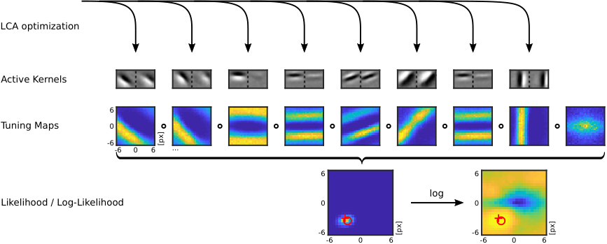
The readout was based on representations obtained by running the LCA procedure on stereo images, but with learning of turned off. The kernels were obtained from the previous LCA optimization on the virtual vergence database. An example of disparity readout is visualized in Fig. 4. With each image presentation, the set of feature maps was used for inference. After settled optimization, the coefficients of all feature maps were set to binary states by applying , with if and otherwise. Disparity was inferred based on the coefficients of feature maps , which is the extend of all coefficients that include a single pixel in their receptive fields. Surface orientation tuning was examined based on a larger region around the central fixation point.
Each category in is represented by a unique two-dimensional parameter combination: horizontal and vertical disparity and , and surface tilt- and slant angles and . At each image location, they can be estimated by selecting for some that is most probable. Assuming independence of the coefficients, estimates were calculated by applying a naïve Bayes classifier with55 5 In practice, inference was calculated equivalently with the logarithmic form .
| (10) |
We omitted the priors , even though a strongly non-uniform distribution of disparities is apparent in natural image data, as can be seen in Fig. 2.
Because elements were restricted to two states, the probabilities of being in one of these states, and were determined experimentally by calculating the arithmetic mean. In the case of stereo disparity, we assumed that the probabilities were linked to each of the kernels and invariant with respect to image feature location. Therefore, probes were accumulated over the feature maps of size , as well as over the whole training set of size by calculating
| (11) |
For inference with Eq. 10, the same probability estimate of one kernel was used for all locations .
In contrast, we assumed that probabilities differ with respect to image location in the case of surface orientation. We reasoned that kernels are mainly disparity tuned and that the orientation of a surface may be detected by the pattern of disparities within a local range. We therefore calculated probability estimates independently for all locations with
| (12) |
Probability estimates vary smoothly with respect to the parameter combinations and as well as for and and therefore constitute “tuning maps”. In the case of surface orientation estimation we exploited this local continuity and smoothed out noise with two dimensional Savitzky-Golay filtering [Savitzky & Golay 1964], with a polynomial of degree , and with px width in both dimensions.
4.4 Linking the processing pipeline to biological vision
With this study, we hope to contribute to a better understanding of biological vision. We chose the aspects of our processing model so that we could study our hypothesis adequately. Here, we motivate some aspects of the simplified naturalistic processing stream, both with respect to biological findings, as well as to their functional role.
Vergence. As a first processing step, we incorporated vergence in our model, the rotation of the two eyes towards each other. The visual system controls gaze, so that the image of objects or any structure of interest is moved to the fovea, the location on the retina with the best spatial resolution. Vergence is not used in common technical solutions. State-of-the-art algorithms work with images obtained with parallel camera axes. They calculate depth by applying epipolar stereo geometry to corresponding locations in both half-images [Hartley & Zisserman 2004]. However, if the goal is to understand vision based on statistical processing, vergence has crucial impact.
Sparse coding is an optimization that builds on statistical regularities of the underlying data. As a first approximation of stereo vision, each half-image is a locally shifted version of the other. The extend of these image shifts, or disparities, differs broadly over the whole scene. In contrast, if both eyes are oriented towards the same location, the distribution of disparities in the vicinity of the fixation point is very narrowly distributed around zero, as shown in Fig. 2. This finding is due to the local smoothness of disparities, disrupted only by discontinuities at object boundaries. Only through vergence the sparse coding algorithm can find statistical dependencies between the two half-images, because corresponding image locations are close-by. Statistical dependencies then manifest in similarly shaped left and right half-kernels, which are often slightly shifted versions of one another. Indeed, Hunt et al. 2013 have shown that sparse coding with simulated strabismus only extracts monocular dominant kernels.
Retinal pre-processing. Receptive fields of the retina are characterized by a center surround organization, with weights in central location that are opposed in polarity to the weights around the center. They are often modeled with the Mexican hat shaped Laplacian of a Gaussian, or the simpler approximation with the difference of two Gaussians, like in our case. Reasons discussed for this kind of retinal processing include mechanisms of efficient coding, compression, response equalization, sparseness and others [Graham et al. 2006]. Convolving the visual input with a difference-of-Gaussians decorrelates the overall pink-noise spectrum of natural scenes, transforming it into a representation with equalized power spectrum [Atick & Redlich 1992]. Removing these first order correlations, also called whitening, is a common pre-processing step before applying an ICA procedure, because it affects the algorithms’ search for higher order statistical dependencies [Hyvärinen & Oja 2000].
Sparse coding in biological substrate. The sparse coding algorithm serves as a model for the formation of neuronal circuitry in V1. It has been proposed that the gradient descent on the error function, with respect to the coefficients, could be implemented directly in neural network topology [Olshausen & Field 1997, Olshausen 2003, Rozell et al. 2008]. In the following, we consider single neurons for simplicity. The gradient descent on coefficients , which is the activity of the neurons in neural network notion, follows a differential equation. In each time step, the activity of a neuron changes proportionally to the sum of three terms (see also Fig. 3): (i.) a feed forward term , where the vectorized kernels serve as receptive fields for the input , (ii.) a competition term that introduces lateral inhibition proportional to the activity from all other neurons of the LCA layer, with weights proportional to the similarity of the receptive fields, and (iii.) a self-inhibition term . In LCA optimization, the sparse coding algorithm is extended by deriving a “leaky integrator” neuron (see Abbott 1999). The main difference is the introduction of an inner state , which is coupled to the output of the neuron with a thresholding function . The three terms stay the same with LCA sparse coding, except that they drive the inner state of the neuron and that the self inhibition in term iii. is replaced by , the leak of the neuron.
This network is reminiscent to the Hopfield network [Little 1974, Hopfield 1982, Hopfield 1984]. With equivalent topology, the weights of networks derived from the Hopfield network are in many cases trained by applying biologically more plausible learning rules that rely on information available at the synapse. For example, Földiak presented an artificial neural network in which feed-forward weights were learned by Hebb’s rule and lateral inhibition was subject to anti-Hebbian learning. Anti-Hebbian learning means that inhibitory connections between neurons were enhanced if they were active at the same time [Földiák 1990]. Therefore, the network learned competition between neurons that were driven by similar patterns, akin to term ii. It was shown that a network with these learning rules, applied to natural images, developes Gabor-like kernels [Falconbridge et al. 2006]. Applying the same Hebbian, anti-Hebbian learning to spiking neural networks yields similar results, drawing even closer to a biologically accurate model [Zylberberg et al. 2011, King et al. 2013]. Chauhan et al. 2018 applied such a network to stereo images and reported successful disparity readout of the neural population with a simple classifier. Physiological studies indeed provide evidence for lateral inhibition between neurons with similar receptive fields in V1: orientation selectivity of neurons might benefit from lateral inhibition between neurons with similar orientation tuning [Blakemore & Tobin 1972] or from other types of cross-orientation inhibition [Ringach 2003, Shapley et al. 2003].
Probabilistic inference. Hypotheses on properties of the world are subject to uncertainty. Bayesian inference provides a framework that allows to account for ambiguity and a broad range of brain functions, like multimodal perception, decision making or motor control, have been modeled following Bayesian approaches [Knill & Pouget 2004, Doya et al. 2006]. Training a perceptron-like neural network with backpropagation is linked to probabilistic inference. With respect to stereo vision, Goncalves & Welchman 2017 analyzed the relationship between a binocular likelihood model and a two layer feed-forward neural network. The first layer represented simple cells, preset with Gabor-like receptive fields, and the second layer represented complex cells tuned for disparities. The weights of both layers were trained with back-propagation. The learned weights from simple to complex cells werer proportional to the log-probability of the simple cell being active, given the preferred disparity represented by the complex cell. Because neural networks of this kind compute the weighed sum of the individual units’ activities, each complex cell calculated the log-likelihood of its preferred disparity. This is equivalent to the naïve Bayes classifier we used for inferring disparity, the logarithmic form of which can be implemented similarly in a neural network.
5 Results
Our analysis of the stereo-vision processing pipeline followed the main hypothesis of this paper: that patterns from the external world can be accessed with simple readout from a representation obtained with sparse coding. We chose disparity and surface orientation as candidates for such patterns. In Sec. 5.1, we first describe qualitative and quantitative properties of the learned LCA representation. Sec. 5.2 addresses the main hypothesis of the paper by evaluating the errors of simple readout of stereo disparity. In Sec. 5.2.1 and 5.2.2 we discuss the extend of errors subject to overcompleteness and sparsity of the LCA representation. The findings are expanded with Sec. 5.2.3, where we describe how the accuracy of the inference can be predicted by the overall activity in the LCA layer. The mechanism holds implications for possible attention mechanisms. Results from these subsections culminate in the evaluation of disparity maps of naturalistic scenes in Sec. 5.2.4. In Sec. 5.3 we then evaluate the orientation tuning of Kernels obtained by LCA optimization.

5.1 Characteristics of the LCA representation
In the following, we focus on results specific to disparity selectivity and compare them to physiological findings. As outlined in Sec. 2.3, the kernels obtained by applying ICA methods to stereo image data have been well described elsewhere. We therefore limit our report to results specific to LCA sparse coding.
5.1.1 Selectivity for disparity
For simple probabilistic readout, individual neurons need to exhibit some degree of specificity for the pattern of interest. Indeed, all tuning maps of kernels obtained with Eq. 11 yielded clear, smoothly varying selectivity as a function of disparity. This was true throughout all kernels obtained by optimizing Eq. 7, irrespective of the level of overcompleteness. Therefore, all kernels potentially contribute to disparity inference with the simple readout scheme. For representative examples, see Figs. 4, 5 and 7. We include all learned kernels in the supplementary material, Figs. S01–S05. The shape of the kernels was in most cases well described by the Gabor function (see Sec. 5.1.2 and Fig. 8a, c). Kernels which were not Gabor-shaped, and which were therefore not classical in terms of physiologically described receptive fields, did only emerge with higher levels of overcompleteness.
We identified three main types of kernel shapes: “Matched Gabor”, “Tuned Inhibitory” and “Blob-like”. A significant number of the “Matched Gabor” and the “Tuned Inhibitory” type were evident at all levels of overcompleteness. However, the share of the “Tuned Inhibitory” type was decreasing the larger the overcompleteness of the model. The “Blob-like” type only emerged in models which were at least overcomplete, with increasing share the larger the overcompleteness of the model. When presented with natural stereo images, the average number of kernels from each type that contributed to the reconstruction of the stimulus was proportional to their share in the set of kernels. This finding was slightly violated if the sparsity penalty was very high. In these cases, “Matched Gabor” kernels had an up to % larger share on the number of active kernels than on average. The three types will be described in more detail in the following paragraphs. For examples of each type see Fig. 5, for the share of each type on the total number of kernels see Fig. 6.
Matched Gabor
The majority of kernels were Gabor-like, with very similar left and right shapes. Differences between the two half-kernels were best described by a shift in position and almost no shift in phase. Tsao et al. 2003 reported that most receptive field shapes in V1 are also characterized by only a small amount of phase-shifts. Such kernels are well suited to represent corresponding (or matching) structures in the two half-images that originate from the same object in the world (see also Sec. 2.4). Conversely, the mode of the tuning maps was equal to the position-shift of the two half-kernels. Note that the mode was sharply peaked perpendicular to the orientation of the kernel shape, but wide in direction of the orientation. These kernels were therefore only selective for disparity perpendicular to their orientation.
Tuned Inhibitory
The probability of these kernels being active increased with the absolute value of disparity. Typically, they were monocular or monocular dominant, i.e., most of the weight energy was in either the left or the right half-kernel. If they were binocular, the lobes were usually shifted by about or by about radians (see also Sec. 5.1.2). Such kernels were also reported by Hunter & Hibbard 2015, see Sec. 2.3. Note that phase-shift kernels might serve as “what not”-detectors when used for stereo inference, as described in Sec. 2.4 [Read & Cumming 2007, Goncalves & Welchman 2017]. The weights of monocular kernels process information from only one stereo half-image. An explanation for the disparity selectivity based on feed forward processing is therefore unlikely. With sparse optimization on the other hand, matching structures can be reconstructed more sparsely with a single binocular kernel, where otherwise two monocular kernels would be needed. In neural network notion, monocular and binocular kernels compete against each other through lateral inhibition. The probability that a binocular kernel exists that can jointly represent both half-images decreases with larger disparities (see Fig. 10). Therefore, the likelihood that monocular kernels are active increases with disparity.
Blob-like
The shapes of this type were not Gabor-like, but had in common a center-surround organization with a central spot of one polarity and a surrounding structure with opposed polarity. The surrounding lobe, however, varied in its extend, not always completely enclosing the central spot. The resulting shapes described a continuum, with a partial opening resembling an end-stopped ridge, an opening of approximately half extend matching a corner and an even further opening describing slightly curved edges. Kernels of this type were selective for disparity in both dimensions, as opposed to Gabor-like kernels, which were prone to the aperture problem: the displacement of an oriented structure can only be measured perpendicular to its orientation. Our results reflect image statistics and therefore show that natural images consist of a substantial amount of structures, which are best described as corners, ridges and blobs. Such elements may be used to reconstruct two-dimensionally displaced structures directly rather than with a combination of local spatial frequency elements, i.e. Gabor-like kernels. Note that Ringach 2002 reported a substantial amount of blob-like receptive field shapes in V1.

The kernel shapes we obtained with LCA sparse coding fit well to physiological findings. Poggio et al. 1988 recorded neuron responses from rhesus macaque monkey visual cortex and classified disparity tuned cells in six categories. Three of these, “Tuned Near”, “Tuned Zero” and “Tuned Far” neurons, were characterized by sharply peaked response curves, tuned to negative, zero or positive horizontal disparities. The two categories “Near” and “Far” contained neurons that were similarly selective for negative or positive disparities. However, these neurons’ responses were not as peaked as the responses of the “Tuned” neurons but rather broadly tuned. The last category was referred to as “Tuned inhibitory” and contained neurons that were more likely to fire the larger the disparity, irrespective of its sign. We can reproduce the physiological examples of all six categories with our kernel sets and present them in Fig. 7.
The three “Tuned” types describe the same response as our “Matched Gabor” kernels. They were sharply tuned to disparity, but only perpendicular to their orientation. If oriented vertically, they were therefore sharply tuned to horizontal disparity. In some cases they were tuned to more than one disparity, like in the second “Matched Gabor” example of Fig. 5. This was due to the repetitions of the sinusoids. However, most of our kernels had a single sinusoid lobe, like in the “Tuned Zero” and “Tuned Far” examples of Fig. 7, which resulted in a single, elongated peak in the tuning maps. It seems that single lobed kernels are a specialty of LCA sparse coding, as compared to standard sparse coding. This finding will be discussed in more detail in Sec. 5.1.2 (see also Fig. 8h).
We also found tuning maps which reproduce the “Near”- and “Far” types. Oblique “Matched Gabor” kernels were more broadly tuned to horizontal disparity, which was due to the kernels’ elongated response peaks in two-dimensional disparity space. However, we reproduced the horizontal tuning curves with shifted images, which was a very stable stimulus. We assume that horizontal disparity tuning of oblique kernels is very sensitive to small changes of vertical disparity. In addition, Poggio & Fischer 1977 found that most “Near”- and “Far” cells received unbalanced inputs from the two eyes, which is not true for our “Matched Gabor” kernels.
The “Tuned Inhibitory” type matches our own classification. In the respective paragraph we have offered an explanation for how the lateral inhibition of the sparse optimization leads to tuned inhibitory units. This finding has physiological support. Poggio & Fischer 1977 and Poggio & Talbot 1981 reported that “Tuned Inhibitory” neurons often showed “strong excitatory dominance of one eye (ocular unbalance), the ‘silent’ eye exercising only inhibitory functions and only over a restricted disparity range”. They also reported bidirectional cells, “with balanced ocularity, from which stimulation of either eye alone evoked excitatory responses that of the two eyes together evident response suppression”. These bidirectional cell’s responses were similar to the response of kernels with about radians shifted sinusoid. Further physiological evidence supports that suppressive mechanisms of this kind help to solve the stereo correspondence problem [Tanabe et al. 2011, Tanabe & Cumming 2014, Henriksen et al. 2016]. To the best of our knowledge, tuned inhibitory units in stereo vision have not been described in the context of sparse coding in the literature, yet.
5.1.2 Statistical analyses of the kernels
In order to characterize quantitative properties of the kernels from the LCA optimization, we fitted the Gabor-function
| (13) |
to each half-kernel , with offset , scale , an elliptical Gaussian envelope and a sinusoid along , with spatial frequency and phase-shift . Orientation and position , in image space were free, with
| (14) |
The elliptical envelope, with widths and , was allowed to rotate freely by the angle , relative to the orientation of the sinusoid, with
| (15) |
We used a custom implementation in MATLAB, which we made publicly available66 6 https://www.mathworks.com/matlabcentral/fileexchange/60700-fit2dgabor-data-options.
Most kernels were well described by the Gabor function, with the coefficient of determination close to (Fig. 8a, c). Some of the lower values can be attributed to monocular kernels, in which the half-kernel with less weight energy has a lower signal-to-noise ratio. With higher levels of overcompleteness, more non-Gabor-like kernel shapes appeared, which is apparent with the heavy tail in the distribution of the overcomplete model ( kernels) in Fig. 8c, as opposed to the distribution of the overcomplete model ( kernels) in Fig. 8a.
We analyzed the ocular dominance of the kernels by adapting the point scale from Hubel and Wiesel [Hubel & Wiesel 1962]. They were calculated with
| (16) |
with values in the range plotted in a histogram with equally spaced bins. Kernels which were left or right monocular fell into category and , respectively. If weight energy was equally distributed, kernels fell into category , the other categories were left or right dominant, respectively. We show the results in Fig. 8b and d. The majority of kernels were in category , i.e., binocular with balanced weight energy (see Fig. 8b, d). A substantial fraction of kernels was purely monocular (category or ). Only a small fraction was in the intermediate categories and the proportion of intermediate kernels was even lower with higher levels of overcompleteness. The shape of these kernels was usually characterized by a phase-shift of about radians. Kernels that did not fall into category were usually of the “Tuned Inhibitory” type, described in Sec. 5.1.1. In physiological experiments, a similar three-mode distribution of weight energy between left and right receptive fields was also found in ferrets, albeit not as distinctly peaked as in our results. [Kalberlah et al. 2009]. Other physiological studies on various animals report rather flat distributions [Schiller et al. 1976, Hubel & Wiesel 1962, Levay et al. 1978, Guillemot et al. 1993, Hubel et al. 2015].
The following analyses were based on the overcomplete model. Fits with a coefficient of determination of were excluded in order to exclude non-classical receptive field shapes. The distribution of orientations (Fig. 8e) had two peaks at degrees and at degrees. Two possible explanations have been offered in the literature for this bias: the rasterization of the input images and the prevalence of orientations in human made structures [Hunt et al. 2013]. The distribution of phases (Fig. 8f) had distinct peeks at degrees, at degrees and at degrees, i.e., the kernel shapes were, in most cases, either sine-like or cosine-like. Ringach 2002 reported that physiological receptive fields similarly cluster in such even- and odd-symmetric shapes. Opposed to our findings with LCA sparse coding, he also reported that, with standard sparse coding, there is a tendency towards odd-symmetric receptive fields, but not towards even-symmetric receptive fields.
As described in Sec. 2.4, binocular Gabor-filters that are shifted in position from left to right half-kernel can serve as matched filters for corresponding image structures, whereas Gabor-filters shifted in phase can serve as “what not”-detectors for false matches [Read & Cumming 2007, Goncalves & Welchman 2017]. We were therefore interested in the interrelationship between the shift in position and the shift in phase of the kernels in our data. Results are displayed in Fig.8g. Because the tuning maps were characterized by elongated peaks, we expressed the position-shift relative to the most sharply tuned axis. It was therefore calculated as the difference in horizontal and vertical position, projected on the axis perpendicular to the orientation of the Gabor function. For better comparability between position-shift and phase-shift, we also normalized the position-shift by the spatial frequency of the sinusoid. The position-shift was therefore calculated as . Our data showed a transient separation between position-shift and phase-shift kernels. If a kernel had both, a substantial position- and phase-shift, they counteracted each other, so that almost all data points fell into quadrant ii and iv. Lobes of the sinusoid match when data points are on the red line. The majority of the kernels was mainly shifted in position and therefore match the “Matched Gabor” type from Sec. 5.1.1.
Ringach 2002 reported that Gabor-like receptive field shapes of macaque V1 were more variable and often more blob-like than kernels from sparse coding and basis vectors from ICA. In his study, he related the spatial frequency of the sinusoid to the extend of the Gaussian envelope , perpendicular to the orientation of the sinusoid, and , along the orientation of the sinusoid. The relationship was lower on average in physiologically measured receptive fields. In Fig. 8h, we show an overlay of the data adapted from Ringach 2002 (macaque V1, black circles), and from Jones & Palmer 1987 (cat V1, black crosses), with our data (blue dots). In this case, we fit the Gabor-functions with the orientation of the elliptical Gaussian envelope fixed at degrees. While standard sparse coding and ICA results in values for the majority of kernels / basis vectors, many kernels from convolutional LCA sparse coding were characterized by lower values. Note that we bound the fitting procedure to and did therefore not allow blob-like fits, so that these kernels do not appear in the panel. The plot also shows that physiological receptive fields, as well as the LCA kernels, had a tendency for , which was not true for standard sparse coding and ICA, as reported by Ringach. Kernels with small values for , i.e., with a small extend of the Gaussian envelope perpendicular to their orientation, are better suited for disparity inference. If the kernel shape consisted of only one sinusoidal lobe (), the associated tuning map had a single elongated peak, as opposed to kernels with more than one sinusoidal lobe, which had multiple, parallel, elongated peaks. The disparity they represented was therefore not ambiguous. Indeed, we observed aliasing effects in the disparity inference if image structures were represented by multi-lobe kernels. For examples, see both “Matched Gabor”-kernels from Fig. 5.
5.2 Evaluation of disparity inference

In this subsection we evaluate whether disparities can successfully be obtained with simple readout from the LCA representation. We explored the limitations by means of the error of the estimates. Inference of disparity was carried out with the full processing pipeline, subject to overcompleteness and sparsity penalty in the LCA optimization as described in Sec. 4.2, and with probabilistic readout as described in Sec. 4.3. The mean absolute errors (MAE) of the estimates were calculated with
| (17) |
where and were the ground truth and the the estimate, respectively. In Sec. 5.2.1–5.2.3, we report the MAE of the disparity estimates . Inference was carried out on the test set from the disparity database with shifted images, described in detail in Sec. 3.2. In Sec. 5.2.4 we report results on inference of horizontal disparity in naturalistic stereo images.
5.2.1 Higher dimensionality extends the set of detectable patterns
An increase of overcompleteness generally resulted in a decrease of disparity inference errors. The best parameter combination from our evaluation ( overcomplete, ) allowed for a mean disparity error below px, measured within the range of – px ground truth absolute disparity (Fig. 9, right panel). Inference was better for small disparities than for large disparities. The same model performed with an error of px for disparity of px horizontally and px vertically. The bias was generally small (data not shown) and apparent only at large disparities close to the cut-off at px.
Overcompleteness had its main impact on the range of disparities for which the model performed well. With small overcompleteness, the error increased much more rapidly with the value of disparity. For example, the overcomplete model with evaluated with an error below px within the range of px disparity but with an error px at px horizontal and vertical disparity (Fig. 9, left panel). We show all parameter combinations we tested in the overview in Fig. 11. The same data is shown as line plots in supplementary Figs. S01–S06. For low levels of overcompleteness ( px, left-hand column of the plot), error dependency on overcompleteness is negligible, whereas for large overcompleteness ( px, right-hand column), overcompleteness has a substantial effect.
This finding was due to qualitative differences in the sets of learned kernels. With larger overcompleteness, more kernels existed with larger position-shift, i.e., with the differences in position between left and right half-kernel (Fig. 10). The distribution of the kernels’ disparity was roughly similar to the distribution of disparities in stereo images (see Fig. 2), with many kernels that represent small disparities and few kernels that represent large disparities. We conclude that, with more overcompleteness, sparse coding extends the set of patterns that are represented explicitly, ordered by the frequency of their occurrence.
5.2.2 Less sparsity results in lower errors

The sparsity load was generally linked to better inference the lower its value. Up to a limit of very low values for , this is true for all levels of overcompleteness and for all ground truth values of disparity, as can be seen in the top row of Fig. 11. Our results are in line with the results from Rigamonti et al. 2011 and from Gardner-Medwin & Barlow 2001 (see Sec. 2). The bottom row of Fig. 11 contains the same data as the top row, but with the sparsity load mapped to the mean number of active coefficients. Activity was roughly linked by a negative exponential to the range of we tested.
In all models except the overcomplete model, we observed slightly increasing errors if sparsity load was very low. For most combinations of overcompleteness and disparity that we evaluated, the lowest mean error was measured at . The error was below in all cases but one—the overcomplete model, measured at px horizontal disparity and px vertical disparity. The minima can be examined in detail in the supplementary Figs. S01–S06. We therefore reject the hypothesis that inference is optimal if the sparsity penalty used during testing matches that used during training. A possible explanation is based on the fact that a binary multi channel code carries most information if the probability of the coefficients to be in one of both states is and independent of other dimensions. [Shannon 1948]. Therefore, assuming that the coefficients were independent, the code carried most information if half of the coefficients were in an active state on average ( for overcomplete, for overcomplete, and for overcomplete). Inference was best slightly below these numbers, which shows in the bottom row of Fig. 11. It was not possible to confirm this finding for larger overcompleteness or larger values of , because very high sparsity load was computationally prohibitive.
The reasoning that Shannon information is the limiting factor is ambivalent. On the one hand, imposing less weight on sparsity in Eq. 7 in turn imposes more weight on the reconstruction constraint, and therefore the preservation of information. On the other hand, information of an overcomplete representation is highly redundant. It is opposed to a compressed code that maximizes Shannon entropy [Field 1994]. However, we binarized the output of the LCA sparse coding before inference, which removed much information from each dimension. Therefore, information content was strongly limited if only a few coefficients were in an active state.

5.2.3 The number of active LCA coefficients predicts the accuracy of inference
We encountered a strong relation between the success of disparity inference and the number of active coefficients. We assessed this relation by sorting responses to examples from the disparity database test set, ordered by the number of active LCA coefficients . The data were binned with a window size of at least data points. Note that the bin size was unequal, due to this constraint. Finally, we calculated percentiles of the MAE of disparity inference. Resulting histograms are shown as the red lines in Fig. 12. The data points of the disparity inference error are plotted in the same diagram, with a heatmap overlay that displays density where the point cloud is very dense (arbitrary units).
The median error as a function of the number of active coefficients was u-shaped. Therefore, inference was best when an average number of coefficients was in an active state. A low number, as well as a large number of active coefficients was a predictor for large errors (Fig. 12, left panel). With a large value of sparsity load , the number of active coefficients was greatly reduced (right panel). In this case, the median error was monotonically decreasing as a function of the number of active coefficients.
We assume that a low number of active coefficients was associated to large errors because the few tuning maps did not contain enough information for accurate inference. The finding could simply account for the absence of structure in the image. An explanation for the association of a large number of active coefficients with large errors is not so straight forward. We hypothesize that the sparse optimization was not able to settle on a good representation and therefore reconstructed the input with much more kernels than on average. These kernels were not well suited for the given image structures and therefore only active due to the lack of better representatives. Our perspective is linked to a study from Froudarakis et al. 2014. They report that the stimulation with phase scrambled movies activates mouse V1 more strongly than the stimulation with natural movies. Simultaneous recordings from a large population of cells were analyzed for discriminability of the presented movies with a linear classifier. Similar to our finding, strong activation was a predictor for bad classification performance.
5.2.4 Disparity map of a naturalistic scene
In addition to inference with constant disparity, i.e., with shifted images, we evaluated our visual processing pipeline with a naturalistic scene from the Genua Pesto database [Canessa et al. 2017]. We present results from one of the scenes in Fig. 13. It consists of disparities in the interval px, as opposed to our model, which is limited to inference in the interval px. We faced the limitation of the model with a scale-space approach, by downsampling the input image to %, %, % and %. Inference was then only evaluated within the interval px at each of these four scales, and with the best available spatial resolution at each location. Image locations outside the interval were excluded beforehand. All experiments were carried out with the overcomplete, model.
Disparity was inferred well within the aforementioned limitations. The disparity map we obtained is shown in Fig. 13c (compare to ground truth disparity map in Fig. 13a). Note that the map is an overlay of the four scales, with best spatial resolution close to the horopter. We chose to plot the predicted error (Fig. 13d) as the th percentile of the error as a function of the number of active coefficients, as described in Sec. 5.2.3. Errors in subplots d–f are relative to the scale , , , and . Fig. 13e is an overlay of the disparity map with the predicted error. The prediction corresponds to clearly identifiable structures in the image. Large errors were predicted for the loudspeakers, for the table texture, and for uniformly colored locations on the monitor. Low errors were predicted for the telephone, for the bags on the right, and for the icons on the monitor. Fig. 13f visualizes the predicted error and the actual error with respect to ground truth disparity in one plot. If prediction failed, this was mostly due to occlusion boundaries. Note that occlusion boundaries were not part of the training, so this type of error can not be attributed to the lack of representation in the LCA optimization.
5.3 Tuning maps of surface orientation

We showed that a representation formed by LCA sparse coding forms a suitable basis to infer stereo disparity. However, we hypothesized that sparse coding fulfills the requirement for simple readout of a much larger set of patterns. As a second example, we examined tuning maps for tilt- and slant angles and of a textured surface (see Sec. 2.4). Results were based on the test set from the surface orientation database, described in detail in Sec. 3.2.
We created tuning maps, not only for each kernel , but for each of entries from the convolutional feature maps with central fixation point. This decision was based on the expectation that the tuning maps were affected by the disparity tuning of the kernels. We reasoned that surface orientation could be inferred from a set of disparity measurements at positions relative to the fixation point. In Fig. 14 we show that kernels were tuned for surface tilt- and slant angles. Indeed, the tuning maps of the kernels differed, depending on the position at which it was evaluated. The peak of the tuning maps was the sharper the larger the slant angle of the surface. In tilt-/slant space, the peak described a skewed band, which was expected if disparity tuning was the underlying principle.
Coefficients in the center of the tuning maps, which corresponded to the fixation point, were also clearly tuned for the surface tilt angle (see central tuning map of Fig. 14 for an example). They could not be affected by disparity because disparity is zero at the fixation point, irrespective of the surface orientation. Instead, the mode of the tuning for the tilt angle was strongly related to the kernels’ orientation , with a circular-circular correlation coefficient (calculated following Jammalamadaka & SenGupta 2001, using CircStat [Berens 2009]). A scatterplot of against is displayed in Fig. 15. Fleming et al. 2004 showed that a set of Gabor-filters can be used to infer surface orientation in monocular images. In images of slanted, textured surfaces, spatial frequencies that are oriented perpendicular to the tilt angle of the surface are overrepresented. This is due to the homographic projection on the retina, which causes an anisotropic compression of surface textures. The finding qualitatively extends the set of patterns that can be inferred from the LCA representation. It adds information to the inference of surface orientation that is different from the inference based on the local distribution of disparities.
6 Discussion
We add evidence to an existent body of literature, which shows that Gabor-like, disparity tuned, phase- and position-shifted receptive fields are a good basis for stereo algorithms (see Sec. 2.3 and 2.4). Simple readout of disparity was possible, due to some degree of selectivity to the stimulus of units from the LCA representation. These units therefore resembled Barlow’s cardinal cells, with intermediate selectivity for the stimulus. Indeed, we did not observe a single kernel that was not tuned for disparity or surface orientation. At the same time, they represented a variety of other stimulus aspects, like spatial frequency, orientation, or blob-like structures. In combination, the kernels represented the input space well and allowed for accurate inference.
6.1 Dimensionality of representations
Larger dimensionality of a representation extended the range of disparities that could be inferred with simple readout. We offer an intuitive explanation for this finding. Local structure in both half-images that originate from the same location in the world can either be represented by one binocular kernel with similar left and right shape; or it can be represented by two kernels: a left and a right monocular kernel. If binocular kernels are available, sparsity can increase substantially, by activation of only half the number of units that would be needed for reconstruction with monocular kernels. However, a representation that contains binocular kernels requires a much larger dimensionality.
Lets assume that we want to create a new binocular representation from monocular kernels, which consists of copies of the same set of monocular half-kernels for each eye. We generate binocular kernels from all monocular kernels, so that the left half-kernels are shifted versions of the right half-kernels. If we assume equally spaced horizontal and vertical shifts in the range , the new representation has kernels, with factor that determines the resolution. Because occlusions are characterized by the lack of corresponding structure, we would have to add the original monocular kernels to the representation, so that the total number of kernels would be . With either set of kernels, the optimization can reconstruct the image equally well, but much more sparsely with the larger set. Obviously, the amount of information is the same in both representations, because the information preservation constraint of the optimization is not affected. However, the larger representation is much more redundant. Interestingly, it is exactly this redundancy that allows for inference, because binocular kernels that fit corresponding features are tuned for disparities.
With large dimensionality, it was possible to infer disparity with binary classification, even though the binarization discards information (compare Bobrowski 2011). Burge and Geisler presented an opposed approach to disparity inference, with very low dimensionality [Burge & Geisler 2014]. They asked which filter shapes were optimal to infer disparity and showed that inference was possible with the two most informative kernels. In their model, the activity ratio of these detectors was the crucial parameter for inference. Information was not distributed over many binary dimensions but encoded in the value of a few dimensions.
In biological systems, the value may be encoded in the firing rates of neurons. Fine grained discriminability between neural activities, i.e., large channel capacity, requires high firing rates. Indeed, there are many examples where neurons encode sensory information with high firing rates. Examples include medial superior olivary neurons, which lock precisely to the phase of pure tones [Brand et al. 2002], and the T-units in Gymnotiforms (weakly electric fish), which lock to the phase of electrical signals with up to almost Hz [Scheich et al. 1973]. Although cortical neurons operate at low mean firing rates of about Hz [Baddeley et al. 1997], action potential bursts are known candidates to encode information in firing rates. For a current review on neural coding with bursts see [Zeldenrust et al. 2018].
6.2 The trade-off between accuracy and energy efficiency
An alternative explanation for the finding that cortical neurons exhibit sparse activity is energy efficiency. The energetic cost of a neuronal population has two major contributions: the maintenance of neurons, which limits population size, and neuronal activity, measured by the average rate of action potentials [Attwell & Laughlin 2001, Lennie 2003]. Because neuronal activity is relatively costly, an optimization that takes energy efficiency into account results in reduced activity [Levy & Baxter 1996].
Indeed, the two terms of the sparse coding optimization Eq. 7 are the preservation of information and the sparsity of the representation, weighted against each other with the sparsity load . We have shown that the mean inference error also depends on . We therefore hypothesize that sparsity in the brain is optimized for the trade-off between the accuracy of upstream processing tasks and energy consumption. This optimization could even occur dynamically and locally, as an attention mechanism that adjusts the error subject to the current task. Such a mechanism could interact with the error prediction we have shown, which relies on counting the number of active coefficients.
The realization in biological substrate is plausible. In neural notion of the LCA sparse coding, the sparsity load corresponds to a shift in the thresholds of neurons (see Sec. 4.4). Indeed, physiological studies show that attentional mechanisms involve changes in the excitability of neurons. McAdams & Maunsell 1999 have shown that attention modulates the response of orientation-tuned neurons in V4 multiplicatively. Similarly, tuning maps of LCA kernels were qualitatively indifferent with respect to . Therefore, an interesting question for future research is whether inference with variable LCA thresholds and static weights for readout is feasible.
6.3 Model-specific issues
Applying our processing pipeline to the naturalistic scene, image locations with disparities larger or smaller than the disparities included in the training set yielded random results. We are confident that an additional category that includes all of the disparities beyond the included range could successfully be added to the training set. The category could rely on activity of coefficients of the “Tuned Inhibitory” type and on lack of activity of the “Matched Gabor” type. Occluded image regions are similarly characterized by the lack of corresponding image structure and might be represented by the same kernel types. Whether it is possible to distinguish between a large-disparity category and an occlusion category is an interesting question for future research.
The resolution of the disparity maps was limited in this study. We used a stride of px for the convolutional LCA sparse coding, which was therefore also the downsampling factor for the disparity map. With the same level of overcompleteness, a larger stride corresponds to a larger number of kernels [Schultz et al. 2014]. We assume that a large number of kernels is mandatory in order to represent a large number of disparities. However, we expect that the resolution of the disparity estimates does not depend on the stride. Tuning maps of coefficients in a single column of the feature maps most likely vary with respect to the position of the image structure in their receptive fields. We may explore the limits of the spatial resolution in future research.
We have presented a naturalistic processing pipeline for disparity inference. Our aim was not to find a method which has the lowest inference error, but to learn more about inference based on sparse representations in general. However, we had reasonable success of inferring disparities in a naturalistic scene. With recent progress on neuromorphic hardware, as well as progress on efficient implementations of the spiking LCA algorithm [Zylberberg et al. 2011, Tang et al. 2017, Watkins et al. 2019], research on the hardware implementation of our biologically inspired stereo vision processing stream would be promising and is within reach.
6.4 Sparse coding and supervision
Because more overcompleteness extends the set of patterns that can be inferred, the set of patterns that is ecologically relevant may predict the extend of the neuronal population in animals. Patterns, too rare to be represented, subject to the cost of neuronal maintenance, should be omitted. The likelihood that sparse coding represents patterns explicitly may depend on the frequency of their occurrence. The distribution might be divergent from the relevance of the patterns an animal needs to detect. Common patterns may be irrelevant while rare patterns, like cues that reveal the attack of a lurking predator, are essential for survival. In the case of depth inference, a uniform accuracy over the whole disparity range might be optimal. An advantageous learning strategy could profit from the generality of feature extraction based on sensory statistics and augment learning with mild supervision in order to gently shift the representation towards a distribution optimized for behavioral gain. In multi-layered networks, later stages might also benefit from incorporating sparsity constraints, by aiding the clustering towards conceptional representations. Current research supports this assumption. Kim et al. 2018 have shown that a standard autoencoder, augmented with lateral inhibition and top-down feedback, develops joined representations of multimodal input data. Hale Berry Neurons were responsive for textual, as well as for visual input. The representation was easily separable and robust for classification tasks.
6.5 The link between image statistics and inference
It remains an open question why a method that extracts statistical properties from natural images yields good features for inference. The original perspective on the independent component analysis (ICA), a class of algorithms to which sparse coding belongs, might point towards a possible explanation. The reasoning behind ICA was that data from sensor arrays are in some cases the weighted superposition of a number of individual, independent source signals [Hyvärinen & Oja 2000]. If the superposition is linear, source signals can be reconstructed by multiplying the vector of sensory data with the inverse of the weight matrix. The aim of ICA is to find this inverse matrix.
Clearly, the assumption that sensory data are the weighted sum of source signals is not true for the formation of two-dimensional images on the retina. Images originate from light rays scattered by objects within a physical, three-dimensional world. The components obtained by ICA are in fact not independent of each other [Bethge 2006, Eichhorn et al. 2009]. They are not the building blocks of an image and the task of inferring depth is not readily solved by extracting these components. However, they seem to coincide with physical causes. The distance of objects manifests in the shift of corresponding image structure, occlusions manifest in the lack of corresponding image structure, and surface orientation manifests in anisotropically compressed texture. Obviously, even though the feature dimensions are not the original components of the image, they are closely linked to the geometrical layout of the scene and therefore allow to infer properties of the external world. They might pose the basis for a heuristic mental model of the external world, established by the clustering of “suspicious coincidences” [Barlow 1987, Földiák 1990].
We believe that the selectivity for patterns that are linked to physical causes is a general property of sparse representations of sensory data. For example, we have recently shown that applying sparse coding to optic flow data yields rather unexpected kernel shapes, which are tuned to directions of egomotion [Ecke et al. 2020]. Screening for such selectivities can be a starting point for identifying the cues that are at the core of inference and it can yield predictions for properties of processing in diverse biological systems.
7 Conclusion
With this study, we have extended the knowledge about similarities and differences between representations learned with stereo sparse coding and the visual cortex. We have also shown that statistical properties of the visual sensory stream can be exploited with the sparse coding algorithm and consecutive simple readout of depth parameters. Disparity can be inferred reasonably well, with very good accuracy for low disparities but with increasing error the larger the disparity. The range of disparities that can be inferred with good accuracy grows with overcompleteness. More sparsity reduces the accuracy of inference. Since neuronal activity is directly associated with energy consumption, attentional mechanisms could optimize the trade-off between energy efficiency and the accuracy needed for the task an animal faces. In addition, we have shown that accuracy of the inference can be inferred from the number of active LCA coefficients itself. The estimate could be used as a feedback parameter to adjust the sparsity of the optimization.
We hypothesized that sparse coding transforms the sensory stream such that an unknown subset of patterns from the external world can be inferred by subsequent, simple readout. After a thorough analysis of disparity inference, we have shown that the representation also carries information that allows to infer surface orientation. Selectivity for this subset of patterns is qualitatively different from disparity tuning because it depends on the orientation of the Gabor-like kernels shapes. We believe that sparse coding generalizes properties from the external world and can be used to infer a much broader range of patterns that are cues for physical causes.
Acknowledgements
This work was carried out at the Department of Biology of the Eberhard-Karls-University, Tübingen, Germany. This research did not receive any specific grant from funding agencies in the public, commercial, or not-for-profit sectors.
References
- Abbott [1999] Abbott, L. F. (1999). Lapicque’s introduction of the integrate-and-fire model neuron (1907). Brain Research Bulletin, 50, 303–304. URL: https://doi.org/10.1016%2Fs0361-9230%2899%2900161-6. doi:doi:10.1016/s0361-9230(99)00161-6. Publisher: Elsevier BV.
- Anzai et al. [1999] Anzai, A., Ohzawa, I., & Freeman, R. D. (1999). Neural mechanisms for encoding binocular disparity: receptive field position versus phase. Journal of Neurophysiology, 82, 874–890. URL: http://jn.physiology.org/content/82/2/874.short. doi:doi:10.1152/jn.1999.82.2.874.
- Atick & Redlich [1992] Atick, J. J., & Redlich, A. N. (1992). What does the retina know about natural scenes? Neural computation, 4, 196–210. doi:doi:10.1162/neco.1992.4.2.196. Number: 2 Reporter: Neural computation.
- Attwell & Laughlin [2001] Attwell, D., & Laughlin, S. B. (2001). An Energy Budget for Signaling in the Grey Matter of the Brain. Journal of Cerebral Blood Flow & Metabolism, 21, 1133–1145. URL: https://doi.org/10.1097%2F00004647-200110000-00001. doi:doi:10.1097/00004647-200110000-00001. Publisher: SAGE Publications.
- Baddeley et al. [1997] Baddeley, R., Abbott, L. F., Booth, M. C. A., Sengpiel, F., Freeman, T., Wakeman, E. A., & Rolls, E. T. (1997). Responses of neurons in primary and inferior temporal visual cortices to natural scenes. Proceedings of the Royal Society of London. Series B: Biological Sciences, 264, 1775–1783. URL: https://doi.org/10.1098%2Frspb.1997.0246. doi:doi:10.1098/rspb.1997.0246.
- Barlow [1987] Barlow, H. (1987). Cerebral Cortex as Model Builder. In L. M. Vaina (Ed.), Matters of Intelligence: Conceptual Structures in Cognitive Neuroscience (pp. 395–406). Dordrecht: Springer Netherlands. URL: https://doi.org/10.1007/978-94-009-3833-5_18. doi:doi:10.1007/978-94-009-3833-5_18 reporter: Matters of Intelligence: Conceptual Structures in Cognitive Neuroscience.
- Barlow [2001a] Barlow, H. (2001a). The exploitation of regularities in the environment by the brain. Behavioral and Brain Sciences, 24. URL: http://www.journals.cambridge.org/abstract_S0140525X01000024. doi:doi:10.1017/S0140525X01000024. Number: 04 Reporter: Behavioral and Brain Sciences.
- Barlow [1959] Barlow, H. B. (1959). Sensory mechanisms, the reduction of redundancy and intelligence. In National Physical Laboratory Symposium No. 10, The Mechanisation of Thought Processes. Her Majesty’s Stationery Office, London.
- Barlow [1972] Barlow, H. B. (1972). Single Units and Sensation: A Neuron Doctrine for Perceptual Psychology? Perception, 1, 371–394. URL: https://doi.org/10.1068%2Fp010371. doi:doi:10.1068/p010371. Number: 4 Reporter: Perception.
- Barlow [2001b] Barlow, H. B. (2001b). Redundancy reduction revisited. Network: Computation in Neural Systems, 12, 241–253. URL: https://doi.org/10.1080%2Fnet.12.3.241.253. doi:doi:10.1080/net.12.3.241.253. Publisher: Informa UK Limited.
- Bay et al. [2008] Bay, H., Ess, A., Tuytelaars, T., & Van Gool, L. (2008). Speeded-up robust features (SURF). Computer vision and image understanding, 110, 346–359. URL: http://www.sciencedirect.com/science/article/pii/S1077314207001555. doi:doi:10.1016/j.cviu.2007.09.014.
- Berens [2009] Berens, P. (2009). CircStat: AMATLABToolbox for Circular Statistics. Journal of Statistical Software, 31. URL: https://doi.org/10.18637%2Fjss.v031.i10. doi:doi:10.18637/jss.v031.i10. Publisher: Foundation for Open Access Statistic.
- Bethge [2006] Bethge, M. (2006). Factorial coding of natural images: how effective are linear models in removing higher-order dependencies? Journal of the Optical Society of America A, 23, 1253. URL: https://doi.org/10.1364%2Fjosaa.23.001253. doi:doi:10.1364/josaa.23.001253. Publisher: The Optical Society.
- Bhatt & Ganguly [2018] Bhatt, V., & Ganguly, U. (2018). Sparsity Enables Data and Energy Efficient Spiking Convolutional Neural Networks. In V. Kůrková, Y. Manolopoulos, B. Hammer, L. Iliadis, & I. Maglogiannis (Eds.), Artificial Neural Networks and Machine Learning – ICANN 2018 (pp. 263–272). Cham: Springer International Publishing volume 11139. URL: http://link.springer.com/10.1007/978-3-030-01418-6_26. doi:doi:10.1007/978-3-030-01418-6_26.
- Blakemore & Tobin [1972] Blakemore, C., & Tobin, E. A. (1972). Lateral inhibition between orientation detectors in the cat’s visual cortex. Experimental Brain Research, 15, 439–440. URL: http://www.springerlink.com/index/J342Q1645P754459.pdf. doi:doi:10.1007/BF00234129. Number: 4 Reporter: Experimental Brain Research.
- Bobrowski [2011] Bobrowski, L. (2011). Induction of Linear Separability through the Ranked Layers of Binary Classifiers. In Engineering Applications of Neural Networks (pp. 69–77). Springer Berlin Heidelberg. URL: https://doi.org/10.1007%2F978-3-642-23957-1_8. doi:doi:10.1007/978-3-642-23957-1_8.
- Brand et al. [2002] Brand, A., Behrend, O., Marquardt, T., McAlpine, D., & Grothe, B. (2002). Precise inhibition is essential for microsecond interaural time difference coding. Nature, 417, 543–547. URL: https://doi.org/10.1038%2F417543a. doi:doi:10.1038/417543a. Publisher: Springer Science and Business Media LLC.
- Burge & Geisler [2014] Burge, J., & Geisler, W. S. (2014). Optimal disparity estimation in natural stereo images. Journal of Vision, 14, 1–1. URL: http://jov.arvojournals.org/Article.aspx?doi=10.1167/14.2.1. doi:doi:10.1167/14.2.1. Number: 2 Reporter: Journal of Vision.
- Canessa et al. [2017] Canessa, A., Gibaldi, A., Chessa, M., Fato, M., Solari, F., & Sabatini, S. P. (2017). A dataset of stereoscopic images and ground-truth disparity mimicking human fixations in peripersonal space. Scientific Data, 4, 170034. URL: http://www.nature.com/articles/sdata201734. doi:doi:10.1038/sdata.2017.34.
- Chauhan et al. [2018] Chauhan, T., Masquelier, T., Montlibert, A., & Cottereau, B. R. (2018). Emergence of Binocular Disparity Selectivity through Hebbian Learning. The Journal of Neuroscience, 38, 9563–9578. URL: https://doi.org/10.1523%2Fjneurosci.1259-18.2018. doi:doi:10.1523/jneurosci.1259-18.2018. Publisher: Society for Neuroscience.
- Doya et al. [2006] Doya, K., Ishii, S., Pouget, A., & Rao, R. P. N. (Eds.) (2006). Bayesian Brain. The MIT Press. URL: https://doi.org/10.7551%2Fmitpress%2F9780262042383.001.0001. doi:doi:10.7551/mitpress/9780262042383.001.0001.
- Ecke et al. [2020] Ecke, G. A., Bruijns, S. A., Hölscher, J., Mikulasch, F. A., Witschel, T., Arrenberg, A. B., & Mallot, H. A. (2020). Sparse coding predicts optic flow specificities of zebrafish pretectal neurons. Neural Computing and Applications, 32, 6745–6754. URL: https://doi.org/10.1007/s00521-019-04500-6. doi:doi:10.1007/s00521-019-04500-6.
- Eichhorn et al. [2009] Eichhorn, J., Sinz, F., & Bethge, M. (2009). Natural Image Coding in V1: How Much Use Is Orientation Selectivity? PLoS Computational Biology, 5, e1000336. URL: https://dx.plos.org/10.1371/journal.pcbi.1000336. doi:doi:10.1371/journal.pcbi.1000336. Number: 4 Reporter: PLoS Computational Biology.
- Falconbridge et al. [2006] Falconbridge, M. S., Stamps, R. L., & Badcock, D. R. (2006). A Simple Hebbian/Anti-Hebbian Network Learns the Sparse, Independent Components of Natural Images. Neural Computation, 18, 415–429. URL: https://doi.org/10.1162%2F089976606775093891. doi:doi:10.1162/089976606775093891. Publisher: MIT Press - Journals.
- Field [1987] Field, D. J. (1987). Relations between the statistics of natural images and the response properties of cortical cells. JOSA A, 4, 2379–2394. URL: https://www.osapublishing.org/abstract.cfm?uri=josaa-4-12-2379. doi:doi:10.1364/JOSAA.4.002379. Number: 12 Reporter: JOSA A.
- Field [1994] Field, D. J. (1994). What Is the Goal of Sensory Coding? Neural Computation, 6, 559–601. URL: https://doi.org/10.1162%2Fneco.1994.6.4.559. doi:doi:10.1162/neco.1994.6.4.559. Publisher: MIT Press - Journals.
- Földiák [1990] Földiák, P. (1990). Forming sparse representations by local anti-Hebbian learning. Biological Cybernetics, 64, 165–170. URL: https://doi.org/10.1007%2Fbf02331346. doi:doi:10.1007/bf02331346. Publisher: Springer Science and Business Media LLC.
- Fleming et al. [2004] Fleming, R. W., Torralba, A., & Adelson, E. H. (2004). Specular reflections and the perception of shape. Journal of Vision, 4, 10. URL: http://jov.arvojournals.org/article.aspx?doi=10.1167/4.9.10. doi:doi:10.1167/4.9.10.
- Froudarakis et al. [2014] Froudarakis, E., Berens, P., Ecker, A. S., Cotton, R. J., Sinz, F. H., Yatsenko, D., Saggau, P., Bethge, M., & Tolias, A. S. (2014). Population code in mouse V1 facilitates readout of natural scenes through increased sparseness. Nature Neuroscience, 17, 851–857. URL: http://www.nature.com/articles/nn.3707. doi:doi:10.1038/nn.3707. Number: 6 Reporter: Nature Neuroscience.
- Gardner-Medwin & Barlow [2001] Gardner-Medwin, A. R., & Barlow, H. B. (2001). The Limits of Counting Accuracy in Distributed Neural Representations. Neural Computation, 13, 477–504. URL: https://doi.org/10.1162%2F089976601300014420. doi:doi:10.1162/089976601300014420. Publisher: MIT Press - Journals.
- Goncalves & Welchman [2017] Goncalves, N. R., & Welchman, A. E. (2017). “What Not” Detectors Help the Brain See in Depth. Current Biology, 27, 1403–1412.e8. URL: http://linkinghub.elsevier.com/retrieve/pii/S0960982217304049. doi:doi:10.1016/j.cub.2017.03.074.
- Graham et al. [2006] Graham, D. J., Chandler, D. M., & Field, D. J. (2006). Can the theory of “whitening” explain the center-surround properties of retinal ganglion cell receptive fields? Vision Research, 46, 2901–2913. URL: http://linkinghub.elsevier.com/retrieve/pii/S0042698906001489. doi:doi:10.1016/j.visres.2006.03.008. Number: 18 Reporter: Vision Research.
- Guillemot et al. [1993] Guillemot, J.-P., Paradis, M.-C., Samson, A., Ptito, M., Richer, L., & Lepore, F. (1993). Binocular interaction and disparity coding in area 19 of visual cortex in normal and split-chiasm cats. Experimental brain research, 94, 405–417. URL: http://link.springer.com/article/10.1007/BF00230199. doi:doi:10.1007/BF00230199.
- Hand & Yu [2001] Hand, D. J., & Yu, K. (2001). Idiot’s Bayes—not so stupid after all? International statistical review, 69, 385–398. URL: https://api.wiley.com/onlinelibrary/tdm/v1/articles/10.1111%2Fj.1751-5823.2001.tb00465.x. doi:doi:10.1111/j.1751-5823.2001.tb00465.x. Publisher: Wiley Online Library.
- Hartley & Zisserman [2004] Hartley, R., & Zisserman, A. (2004). Multiple View Geometry in Computer Vision. Cambridge University Press. URL: https://doi.org/10.1017%2Fcbo9780511811685. doi:doi:10.1017/cbo9780511811685.
- Henriksen et al. [2016] Henriksen, S., Tanabe, S., & Cumming, B. (2016). Disparity processing in primary visual cortex. Philosophical Transactions of the Royal Society B: Biological Sciences, 371, 20150255. URL: http://rstb.royalsocietypublishing.org/lookup/doi/10.1098/rstb.2015.0255. doi:doi:10.1098/rstb.2015.0255.
- Hopfield [1982] Hopfield, J. J. (1982). Neural networks and physical systems with emergent collective computational abilities. Proceedings of the National Academy of Sciences, 79, 2554–2558. URL: https://doi.org/10.1073%2Fpnas.79.8.2554. doi:doi:10.1073/pnas.79.8.2554. Publisher: Proceedings of the National Academy of Sciences.
- Hopfield [1984] Hopfield, J. J. (1984). Neurons with graded response have collective computational properties like those of two-state neurons. Proceedings of the national academy of sciences, 81, 3088–3092. URL: https://doi.org/10.1073/pnas.81.10.3088. doi:doi:10.1073/pnas.81.10.3088.
- Hoyer & Hyvärinen [2000] Hoyer, P. O., & Hyvärinen, A. (2000). Independent component analysis applied to feature extraction from colour and stereo images. Network: Computation in Neural Systems, 11, 191–210. URL: http://informahealthcare.com/doi/abs/10.1088/0954-898X_11_3_302. doi:doi:10.1088/0954-898X_11_3_302. Number: 3 Reporter: Network: Computation in Neural Systems.
- Hubel & Wiesel [1962] Hubel, D. H., & Wiesel, T. N. (1962). Receptive fields, binocular interaction and functional architecture in the cat’s visual cortex. The Journal of physiology, 160, 106–154. URL: http://dx.doi.org/10.1113/jphysiol.1959.sp006308. doi:doi:10.1113/jphysiol.1962.sp006837. Publisher: Wiley Online Library.
- Hubel & Wiesel [1970] Hubel, D. H., & Wiesel, T. N. (1970). Stereoscopic Vision in Macaque Monkey: Cells sensitive to Binocular Depth in Area 18 of the Macaque Monkey Cortex. Nature, 225, 41–42. URL: https://doi.org/10.1038%2F225041a0. doi:doi:10.1038/225041a0.
- Hubel et al. [2015] Hubel, D. H., Wiesel, T. N., Yeagle, E. M., Lafer-Sousa, R., & Conway, B. R. (2015). Binocular Stereoscopy in Visual Areas V-2, V-3, and V-3A of the Macaque Monkey. Cerebral Cortex, 25, 959–971. URL: https://academic.oup.com/cercor/article-lookup/doi/10.1093/cercor/bht288. doi:doi:10.1093/cercor/bht288.
- Hunt et al. [2013] Hunt, J. J., Dayan, P., & Goodhill, G. J. (2013). Sparse Coding Can Predict Primary Visual Cortex Receptive Field Changes Induced by Abnormal Visual Input. PLoS Computational Biology, 9, e1003005. URL: https://doi.org/10.1371%2Fjournal.pcbi.1003005. doi:doi:10.1371/journal.pcbi.1003005.
- Hunter & Hibbard [2015] Hunter, D. W., & Hibbard, P. B. (2015). Distribution of independent components of binocular natural images. Journal of Vision, 15, 6. URL: http://jov.arvojournals.org/article.aspx?doi=10.1167/15.13.6. doi:doi:10.1167/15.13.6. Number: 13 Reporter: Journal of Vision.
- Hyvärinen & Oja [2000] Hyvärinen, A., & Oja, E. (2000). Independent component analysis: algorithms and applications. Neural networks, 13, 411–430. URL: http://www.sciencedirect.com/science/article/pii/S0893608000000265. doi:doi:10.1016/S0893-6080(00)00026-5. Number: 4 Reporter: Neural networks.
- Hyvärinen et al. [1998] Hyvärinen, A., Oja, E., Hoyer, P., & Hurri, J. (1998). Image feature extraction by sparse coding and independent component analysis. In Proceedings. Fourteenth International Conference on Pattern Recognition (Cat. No.98EX170). IEEE Comput. Soc. URL: https://doi.org/10.1109%2Ficpr.1998.711932. doi:doi:10.1109/icpr.1998.711932.
- Ilg et al. [2017] Ilg, E., Mayer, N., Saikia, T., Keuper, M., Dosovitskiy, A., & Brox, T. (2017). FlowNet 2.0: Evolution of Optical Flow Estimation with Deep Networks. In 2017 IEEE Conference on Computer Vision and Pattern Recognition (CVPR). IEEE. URL: https://doi.org/10.1109%2Fcvpr.2017.179. doi:doi:10.1109/cvpr.2017.179.
- Jammalamadaka & SenGupta [2001] Jammalamadaka, S. R., & SenGupta, A. (2001). Topics in Circular Statistics. WORLD SCIENTIFIC. URL: https://doi.org/10.1142%2F4031. doi:doi:10.1142/4031.
- Jones & Palmer [1987] Jones, J. P., & Palmer, L. A. (1987). An evaluation of the two-dimensional Gabor filter model of simple receptive fields in cat striate cortex. Journal of Neurophysiology, 58, 1233–1258. URL: https://doi.org/10.1152%2Fjn.1987.58.6.1233. doi:doi:10.1152/jn.1987.58.6.1233. Publisher: American Physiological Society.
- Kalberlah et al. [2009] Kalberlah, C., Distler, C., & Hoffmann, K.-P. (2009). Sensitivity to relative disparity in early visual cortex of pigmented and albino ferrets. Experimental Brain Research, 192, 379–389. URL: http://link.springer.com/10.1007/s00221-008-1545-z. doi:doi:10.1007/s00221-008-1545-z.
- Kim et al. [2018] Kim, E., Hannan, D., & Kenyon, G. (2018). Deep Sparse Coding for Invariant Multimodal Halle Berry Neurons. In 2018 IEEE/CVF Conference on Computer Vision and Pattern Recognition. IEEE. URL: https://doi.org/10.1109%2Fcvpr.2018.00122. doi:doi:10.1109/cvpr.2018.00122 reporter: 2018 IEEE/CVF Conference on Computer Vision and Pattern Recognition.
- King et al. [2013] King, P. D., Zylberberg, J., & DeWeese, M. R. (2013). Inhibitory Interneurons Decorrelate Excitatory Cells to Drive Sparse Code Formation in a Spiking Model of V1. Journal of Neuroscience, 33, 5475–5485. URL: http://www.jneurosci.org/cgi/doi/10.1523/JNEUROSCI.4188-12.2013. doi:doi:10.1523/JNEUROSCI.4188-12.2013. Number: 13 Reporter: Journal of Neuroscience.
- Knill & Pouget [2004] Knill, D. C., & Pouget, A. (2004). The Bayesian brain: the role of uncertainty in neural coding and computation. Trends in Neurosciences, 27, 712–719. URL: https://doi.org/10.1016%2Fj.tins.2004.10.007. doi:doi:10.1016/j.tins.2004.10.007. Number: 12 Reporter: Trends in Neurosciences Publisher: Elsevier BV.
- Kuncheva [2006] Kuncheva, L. I. (2006). On the optimality of Naïve Bayes with dependent binary features. Pattern Recognition Letters, 27, 830–837. URL: http://linkinghub.elsevier.com/retrieve/pii/S0167865505003582. doi:doi:10.1016/j.patrec.2005.12.001.
- Kupervasser [2014] Kupervasser, O. (2014). The mysterious optimality of Naive Bayes: Estimation of the probability in the system of “classifiers”. Pattern Recognition and Image Analysis, 24, 1–10. URL: http://link.springer.com/10.1134/S1054661814010088. doi:doi:10.1134/S1054661814010088.
- Lennie [2003] Lennie, P. (2003). The Cost of Cortical Computation. Current Biology, 13, 493–497. URL: https://doi.org/10.1016%2Fs0960-9822%2803%2900135-0. doi:doi:10.1016/s0960-9822(03)00135-0. Publisher: Elsevier BV.
- Levay et al. [1978] Levay, S., Stryker, M. P., & Shatz, C. J. (1978). Ocular dominance columns and their development in layer IV of the cat’s visual cortex: a quantitative study. Journal of Comparative Neurology, 179, 223–244. URL: http://dx.doi.org/10.1002/cne.901790113. doi:doi:10.1002/cne.901790113.
- Levy & Baxter [1996] Levy, W. B., & Baxter, R. A. (1996). Energy Efficient Neural Codes. Neural Computation, 8, 531–543. URL: https://doi.org/10.1162%2Fneco.1996.8.3.531. doi:doi:10.1162/neco.1996.8.3.531. Publisher: MIT Press - Journals.
- Li & Atick [1994] Li, Z., & Atick, J. J. (1994). Efficient stereo coding in the multiscale representation. Network: Computation in Neural Systems, 5, 157–174. URL: https://www.tandfonline.com/doi/full/10.1088/0954-898X_5_2_003. doi:doi:10.1088/0954-898X_5_2_003. Number: 2 Reporter: Network: Computation in Neural Systems.
- Little [1974] Little, W. A. (1974). The Existence of Persistent States in the Brain. In From High-Temperature Superconductivity to Microminiature Refrigeration (pp. 145–164). Springer US. URL: https://doi.org/10.1007%2F978-1-4613-0411-1_12. doi:doi:10.1007/978-1-4613-0411-1_12.
- Lonini et al. [2013] Lonini, L., Forestier, S., Teulière, C., Zhao, Y., Shi, B. E., & Triesch, J. (2013). Robust active binocular vision through intrinsically motivated learning. Frontiers in Neurorobotics, 7. URL: http://journal.frontiersin.org/article/10.3389/fnbot.2013.00020/abstract. doi:doi:10.3389/fnbot.2013.00020. Reporter: Frontiers in Neurorobotics.
- Lopez-Hazas et al. [2018] Lopez-Hazas, J., Montero, A., & Rodriguez, F. B. (2018). Strategies to Enhance Pattern Recognition in Neural Networks Based on the Insect Olfactory System. In V. Kůrková, Y. Manolopoulos, B. Hammer, L. Iliadis, & I. Maglogiannis (Eds.), Artificial Neural Networks and Machine Learning – ICANN 2018 (pp. 468–475). Cham: Springer International Publishing volume 11139. URL: http://link.springer.com/10.1007/978-3-030-01418-6_46. doi:doi:10.1007/978-3-030-01418-6_46.
- Lundquist et al. [2017] Lundquist, S. Y., Mitchell, M., & Kenyon, G. T. (2017). Sparse Coding on Stereo Video for Object Detection. arXiv preprint arXiv:1705.07144, . URL: https://arxiv.org/abs/1705.07144.
- Lundquist et al. [2016] Lundquist, S. Y., Paiton, D. M., Schultz, P. F., & Kenyon, G. T. (2016). Sparse encoding of binocular images for depth inference. In 2016 IEEE Southwest Symposium on Image Analysis and Interpretation (SSIAI). IEEE. URL: https://doi.org/10.1109%2Fssiai.2016.7459190. doi:doi:10.1109/ssiai.2016.7459190.
- Mallot [1999] Mallot, H. A. (1999). Stereopsis: Geometrical and global aspects. In Handbook of computer vision and applications Vol. 2: Signal processing and pattern recognition (pp. 485–502). San Diego: Academic Press. URL: http://citeseerx.ist.psu.edu/viewdoc/download?doi=10.1.1.739.5246&rep=rep1&type=pdf.
- Mallot et al. [1996] Mallot, H. A., Roll, A., & Arndt, P. A. (1996). Disparity-evoked Vergence is Driven by Interocular Correlation. Vision Research, 36, 2925–2937. URL: https://doi.org/10.1016%2F0042-6989%2896%2900011-9. doi:doi:10.1016/0042-6989(96)00011-9. Publisher: Elsevier BV.
- Marr & Poggio [1976] Marr, D., & Poggio, T. (1976). Cooperative computation of stereo disparity. Science, 194, 283–287. URL: https://doi.org/10.1126%2Fscience.968482. doi:doi:10.1126/science.968482.
- Marr & Poggio [1979] Marr, D., & Poggio, T. (1979). A Computational Theory of Human Stereo Vision. Proceedings of the Royal Society B: Biological Sciences, 204, 301–328. URL: https://doi.org/10.1098%2Frspb.1979.0029. doi:doi:10.1098/rspb.1979.0029.
- McAdams & Maunsell [1999] McAdams, C. J., & Maunsell, J. H. R. (1999). Effects of Attention on Orientation-Tuning Functions of Single Neurons in Macaque Cortical Area V4. The Journal of Neuroscience, 19, 431–441. URL: https://doi.org/10.1523%2Fjneurosci.19-01-00431.1999. doi:doi:10.1523/jneurosci.19-01-00431.1999. Publisher: Society for Neuroscience.
- Ohzawa et al. [1990] Ohzawa, I., DeAngelis, G., & Freeman, R. (1990). Stereoscopic depth discrimination in the visual cortex: neurons ideally suited as disparity detectors. Science, 249, 1037–1041. URL: https://doi.org/10.1126%2Fscience.2396096. doi:doi:10.1126/science.2396096. Publisher: American Association for the Advancement of Science (AAAS).
- Olshausen [2003] Olshausen, B. A. (2003). Principles of Image Representation in Visual Cortex. In The visual neurosciences, LM Chalupa, JS Werner, Eds (pp. 1603–1615). MIT Press volume 2. URL: https://groups.oist.jp/sites/default/files/img/ocnc/2004/Olshausen.pdf.
- Olshausen & Field [1996] Olshausen, B. A., & Field, D. J. (1996). Emergence of simple-cell receptive field properties by learning a sparse code for natural images. Nature, 381, 607–609. URL: https://doi.org/10.1038%2F381607a0. doi:doi:10.1038/381607a0. Number: 6583 Reporter: Nature.
- Olshausen & Field [1997] Olshausen, B. A., & Field, D. J. (1997). Sparse coding with an overcomplete basis set: A strategy employed by V1? Vision Research, 37, 3311–3325. URL: https://doi.org/10.1016%2Fs0042-6989%2897%2900169-7. doi:doi:10.1016/s0042-6989(97)00169-7. Number: 23 Reporter: Vision Research.
- Orban [2008] Orban, G. A. (2008). Higher Order Visual Processing in Macaque Extrastriate Cortex. Physiological Reviews, 88, 59–89. URL: http://physrev.physiology.org/cgi/doi/10.1152/physrev.00008.2007. doi:doi:10.1152/physrev.00008.2007.
- Orban [2011] Orban, G. A. (2011). The Extraction of 3D Shape in the Visual System of Human and Nonhuman Primates. Annual Review of Neuroscience, 34, 361–388. URL: http://www.annualreviews.org/doi/abs/10.1146/annurev-neuro-061010-113819. doi:doi:10.1146/annurev-neuro-061010-113819.
- Poggio & Fischer [1977] Poggio, G. F., & Fischer, B. (1977). Binocular interaction and depth sensitivity in striate and prestriate cortex of behaving rhesus monkey. Journal of Neurophysiology, 40, 1392–1405. URL: https://doi.org/10.1152%2Fjn.1977.40.6.1392. doi:doi:10.1152/jn.1977.40.6.1392. Publisher: American Physiological Society.
- Poggio et al. [1988] Poggio, G. F., Gonzalez, F., & Krause, F. (1988). Stereoscopic mechanisms in monkey visual cortex: binocular correlation and disparity selectivity. The Journal of neuroscience, 8, 4531–4550. URL: http://www.jneurosci.org/content/8/12/4531.short. doi:doi:10.1523/JNEUROSCI.08-12-04531.1988.
- Poggio & Talbot [1981] Poggio, G. F., & Talbot, W. H. (1981). Mechanisms of static and dynamic stereopsis in foveal cortex of the rhesus monkey. The Journal of physiology, 315, 469–492. URL: http://onlinelibrary.wiley.com/doi/10.1113/jphysiol.1981.sp013759/full. doi:doi:10.1113/jphysiol.1981.sp013759.
- Read & Cumming [2007] Read, J. C. A., & Cumming, B. G. (2007). Sensors for impossible stimuli may solve the stereo correspondence problem. Nature Neuroscience, 10, 1322–1328. URL: http://www.nature.com/articles/nn1951. doi:doi:10.1038/nn1951.
- Rehn & Sommer [2007] Rehn, M., & Sommer, F. T. (2007). A network that uses few active neurones to code visual input predicts the diverse shapes of cortical receptive fields. Journal of Computational Neuroscience, 22, 135–146. URL: http://link.springer.com/10.1007/s10827-006-0003-9. doi:doi:10.1007/s10827-006-0003-9. Number: 2 Reporter: Journal of Computational Neuroscience.
- Rigamonti et al. [2011] Rigamonti, R., Brown, M. A., & Lepetit, V. (2011). Are sparse representations really relevant for image classification? In CVPR 2011. IEEE. URL: https://doi.org/10.1109%2Fcvpr.2011.5995313. doi:doi:10.1109/cvpr.2011.5995313.
- Ringach [2002] Ringach, D. L. (2002). Spatial Structure and Symmetry of Simple-Cell Receptive Fields in Macaque Primary Visual Cortex. Journal of Neurophysiology, 88, 455–463. URL: https://doi.org/10.1152%2Fjn.2002.88.1.455. doi:doi:10.1152/jn.2002.88.1.455. Publisher: American Physiological Society.
- Ringach [2003] Ringach, D. L. (2003). Dynamics of Orientation Tuning in Macaque V1: The Role of Global and Tuned Suppression. Journal of Neurophysiology, 90, 342–352. URL: http://jn.physiology.org/cgi/doi/10.1152/jn.01018.2002. doi:doi:10.1152/jn.01018.2002.
- Rolls & Tovee [1995] Rolls, E. T., & Tovee, M. J. (1995). Sparseness of the neuronal representation of stimuli in the primate temporal visual cortex. Journal of Neurophysiology, 73, 713–726. URL: https://doi.org/10.1152%2Fjn.1995.73.2.713. doi:doi:10.1152/jn.1995.73.2.713.
- Rozell et al. [2008] Rozell, C. J., Johnson, D. H., Baraniuk, R. G., & Olshausen, B. A. (2008). Sparse Coding via Thresholding and Local Competition in Neural Circuits. Neural Computation, 20, 2526–2563. URL: https://doi.org/10.1162%2Fneco.2008.03-07-486. doi:doi:10.1162/neco.2008.03-07-486. Number: 10 Reporter: Neural Computation.
- Savitzky & Golay [1964] Savitzky, A., & Golay, M. J. E. (1964). Smoothing and Differentiation of Data by Simplified Least Squares Procedures. Analytical Chemistry, 36, 1627–1639. URL: http://pubs.acs.org/doi/abs/10.1021/ac60214a047. doi:doi:10.1021/ac60214a047.
- Scheich et al. [1973] Scheich, H., Bullock, T. H., & Hamstra, R. H. (1973). Coding properties of two classes of afferent nerve fibers: high-frequency electroreceptors in the electric fish, Eigenmannia. Journal of Neurophysiology, 36, 39–60. URL: https://doi.org/10.1152%2Fjn.1973.36.1.39. doi:doi:10.1152/jn.1973.36.1.39. Publisher: American Physiological Society.
- Schiller et al. [1976] Schiller, P. H., Finlay, B. L., & Volman, S. F. (1976). Quantitative studies of single-cell properties in monkey striate cortex. III. Spatial frequency. Journal of Neurophysiology, 39, 1334–1351. URL: https://doi.org/10.1152%2Fjn.1976.39.6.1334. doi:doi:10.1152/jn.1976.39.6.1334. Publisher: American Physiological Society.
- Schultz et al. [2014] Schultz, P. F., Paiton, D. M., Lu, W., & Kenyon, G. T. (2014). Replicating kernels with a short stride allows sparse reconstructions with fewer independent kernels. arXiv preprint arXiv:1406.4205, . URL: http://arxiv.org/abs/1406.4205. Reporter: arXiv preprint arXiv:1406.4205.
- Shannon [1948] Shannon, C. E. (1948). A Mathematical Theory of Communication. Bell System Technical Journal, 27, 623–656. URL: https://doi.org/10.1002%2Fj.1538-7305.1948.tb00917.x. doi:doi:10.1002/j.1538-7305.1948.tb00917.x. Publisher: Institute of Electrical and Electronics Engineers (IEEE).
- Shapley et al. [2003] Shapley, R., Hawken, M., & Ringach, D. L. (2003). Dynamics of orientation selectivity in the primary visual cortex and the importance of cortical inhibition. Neuron, 38, 689–699. URL: https://dx.doi.org/10.1016/S0896-6273(03)00332-5. doi:doi:10.1016/S0896-6273(03)00332-5.
- Simoncelli & Olshausen [2001] Simoncelli, E. P., & Olshausen, B. A. (2001). Natural Image Statistics and Neural Representation. Annual Review of Neuroscience, 24, 1193–1216. URL: https://doi.org/10.1146%2Fannurev.neuro.24.1.1193. doi:doi:10.1146/annurev.neuro.24.1.1193. Publisher: Annual Reviews.
- Tanabe & Cumming [2014] Tanabe, S., & Cumming, B. G. (2014). Delayed suppression shapes disparity selective responses in monkey V1. Journal of Neurophysiology, 111, 1759–1769. URL: http://www.physiology.org/doi/10.1152/jn.00426.2013. doi:doi:10.1152/jn.00426.2013.
- Tanabe et al. [2011] Tanabe, S., Haefner, R. M., & Cumming, B. G. (2011). Suppressive Mechanisms in Monkey V1 Help to Solve the Stereo Correspondence Problem. Journal of Neuroscience, 31, 8295–8305. URL: http://www.jneurosci.org/cgi/doi/10.1523/JNEUROSCI.5000-10.2011. doi:doi:10.1523/JNEUROSCI.5000-10.2011.
- Tang et al. [2017] Tang, P. T. P., Lin, T.-H., & Davies, M. (2017). Sparse coding by spiking neural networks: Convergence theory and computational results. arXiv preprint arXiv:1705.05475, . URL: https://arxiv.org/pdf/1705.05475.pdf.
- Tibshirani [1996] Tibshirani, R. (1996). Regression shrinkage and selection via the lasso. Journal of the Royal Statistical Society. Series B (Methodological), (pp. 267–288). doi:doi:10.1111/j.2517-6161.1996.tb02080.x.
- Timofte & Van Gool [2015] Timofte, R., & Van Gool, L. (2015). Sparse Flow: Sparse Matching for Small to Large Displacement Optical Flow. In 2015 IEEE Winter Conference on Applications of Computer Vision (pp. 1100–1106). IEEE. URL: https://doi.org/10.1109%2Fwacv.2015.151. doi:doi:10.1109/wacv.2015.151.
- Tsao et al. [2003] Tsao, D. Y., Conway, B. R., & Livingstone, M. S. (2003). Receptive fields of disparity-tuned simple cells in macaque V1. Neuron, 38, 103–114. URL: http://www.sciencedirect.com/science/article/pii/S0896627303001508. doi:doi:10.1016/S0896-6273(03)00150-8.
- Watkins et al. [2019] Watkins, Y., Thresher, A., Schultz, P. F., Wild, A., Sornborger, A., & Kenyon, G. T. (2019). Unsupervised Dictionary Learning via a Spiking Locally Competitive Algorithm. In Proceedings of the International Conference on Neuromorphic Systems - ICONS \textquotesingle19. ACM Press. URL: https://doi.org/10.1145%2F3354265.3354276. doi:doi:10.1145/3354265.3354276 reporter: Proceedings of the International Conference on Neuromorphic Systems - ICONS \textquotesingle19.
- Zeiler et al. [2010] Zeiler, M. D., Krishnan, D., Taylor, G. W., & Fergus, R. (2010). Deconvolutional networks. In 2010 IEEE Computer Society Conference on Computer Vision and Pattern Recognition. IEEE. URL: https://doi.org/10.1109%2Fcvpr.2010.5539957. doi:doi:10.1109/cvpr.2010.5539957.
- Zeldenrust et al. [2018] Zeldenrust, F., Wadman, W. J., & Englitz, B. (2018). Neural Coding With Bursts—Current State and Future Perspectives. Frontiers in Computational Neuroscience, 12. URL: https://www.frontiersin.org/article/10.3389/fncom.2018.00048/full. doi:doi:10.3389/fncom.2018.00048.
- Zhang [2005] Zhang, H. (2005). Exploring Conditions for the Optimality of Naïve Bayes. International Journal of Pattern Recognition and Artificial Intelligence, 19, 183–198. URL: http://www.worldscientific.com/doi/abs/10.1142/S0218001405003983. doi:doi:10.1142/S0218001405003983.
- Zylberberg et al. [2011] Zylberberg, J., Murphy, J. T., & DeWeese, M. R. (2011). A Sparse Coding Model with Synaptically Local Plasticity and Spiking Neurons Can Account for the Diverse Shapes of V1 Simple Cell Receptive Fields. PLoS Computational Biology, 7, e1002250. URL: http://dx.plos.org/10.1371/journal.pcbi.1002250. doi:doi:10.1371/journal.pcbi.1002250. Number: 10 Reporter: PLoS Computational Biology.