Kernel regression analysis of tie-breaker designs Thanks: This version of the paper is published in the Electronic Journal of Statistics with open access (DOI: doi.org/10.1214/23-EJS2102). There are formatting differences between the arXiv and journal versions.
Abstract
Tie-breaker experimental designs are hybrids of Randomized Controlled Trials (RCTs) and Regression Discontinuity Designs (RDDs) in which subjects with moderate scores are placed in an RCT while subjects with extreme scores are deterministically assigned to the treatment or control group. In settings where it is unfair or uneconomical to deny the treatment to the more deserving recipients, the tie-breaker design (TBD) trades off the practical advantages of the RDD with the statistical advantages of the RCT. The practical costs of the randomization in TBDs can be hard to quantify in generality, while the statistical benefits conferred by randomization in TBDs have only been studied under linear and quadratic models. In this paper, we discuss and quantify the statistical benefits of TBDs without using parametric modelling assumptions. If the goal is estimation of the average treatment effect or the treatment effect at more than one score value, the statistical benefits of using a TBD over an RDD are apparent. If the goal is nonparametric estimation of the mean treatment effect at merely one score value, we prove that about 2.8 times more subjects are needed for an RDD in order to achieve the same asymptotic mean squared error. We further demonstrate using both theoretical results and simulations from the Angrist and Lavy 1999 classroom size dataset, that larger experimental radii choices for the TBD lead to greater statistical efficiency.
keywords
[class=MSC] Primary 62K99 ; secondary 62G20 , 62G08keywords
causal inference , experimental design , hybrid experiments , local linear regression , regression discontinuity designsand
Department of Statistics, Stanford University, Stanford CA, 94305
??; ??
Contents
1 Introduction
In this paper we study a nonparametric regression approach to tie-breaker studies. In the settings of tie-breaker studies, there is a costly treatment while the control is inexpensive or even free. In addition, an investigator can decide how to allocate the costly treatment using a priority ordering on the subjects. The priority ordering could be based on how deserving of the treatment each subject is, or based on how strongly each subject is expected to respond to the treatment. Examples include offering scholarships or school placement to students (Angrist, Autor and Pallais 2020), offering a drug rehabilitation program to people of varying needs (Cappelleri and Trochim 2003), or assigning interventions to reduce risk factors for child abuse and neglect (Krantz 2022). In these settings a randomized controlled trial (RCT) is inappropriate because it is extremely inefficient economically, or even ethically questionable. The natural, even automatic, approach to settings like this is to rank the subjects according to their value of a running variable and assign the treatment to only those subjects with the highest values of . For simplicity one can assume that the number of subjects to treat is fixed and that the treatment is offered to subject if and only if for some threshold .
The problem with a deterministic treatment based on is that it complicates causal inference of the effect of the treatment. One can use regression discontinuity analysis (Thistlethwaite and Campbell 1960; Cattaneo and Titiunik 2022) but the regression discontinuity design (RDD) is known to give treatment effect estimates a very high variance. See, for example, Gelman and Imbens 2019. In a parametric regression model the treatment and running variable are highly correlated, making for an inefficient design (Goldberger 1972; Jacob et al. 2012). In a tie-breaker design (TBD), the subjects are given the treatment with a probability that increases with . The top ranked subjects get the treatment with probability one, the bottom ranked subjects do not get the treatment and subjects in between are randomly assigned to either treatment or control. The tie-breaker design interpolates between two extremes: the RCT and the RDD, trading off statistical efficiency with the short term economic value of aligning treatment to the running variable.
We believe that there are many more good uses for TBDs. Many companies interact electronically with their customers and partners. Perks, such as service upgrades, can easily be assigned with some randomization. Because the treatment is costly, it is important to evaluate the treatment efficacy later. This provides a strong motivation to introduce randomization. When the perk is simply a gift to some subjects there is less ethical concern over whether it goes to the most loyal customers or introduces some randomization. We also expect that tie-breakers will be useful in evaluating governmental programs such as the one in Krantz 2022, as well as educational programs such as those in Angrist, Autor and Pallais 2020.
TBDs have been primarily studied as experimental designs using parametric regression modeling assumptions. While the design literature focuses on parametric models, the RDD literature primarily uses nonparametric regression methods. In this paper, we quantify the statistical gains to be obtained by conducting a TBD instead of an RDD using nonparametric regression.
Our main theoretical contributions are as follows. We study a kernel weighted local linear regression with a slope and intercept for both treated and control subjects and bandwidth . The RDD can consistently estimate the treatment effect only at , and so we focus our comparison at that point. We find an expression for the optimal bandwidth for estimating the treatment effect at under the TBD. We then compare the optimal mean squared error at for the two designs. For the popular triangular kernel, a TBD reduces the asymptotic mean squared error (AMSE) by a factor of about compared to an RDD of the same sample size, . For other popular kernels, the AMSE is reduced by a slightly greater factor. In this setting, the AMSE decreases proportionally to , and using points in an RDD is comparable to using only points in a TBD. The asymptotic analysis has a bandwidth that converges to zero. Since this convergence is at the very slow rate, we cannot assume that in practice will be small enough such that subjects without randomized treatment are discarded. Therefore, we also compare the designs when is fixed and large enough to include nonnrandomized subjects in the regression. In this setting, the efficiency ratio, which we define as the relative variance of treatment effect estimators under the two designs, can be as large as four. For a fixed bandwidth and for the triangular and boxcar kernels, we also find that the efficiency ratio is monotone non-decreasing in the proportion of subjects who are given a randomized treatment assignment.
A further advantage of the TBD is that it can give consistent nonparametric estimates of the treatment effect for any value of in the randomization window. It can also be used to estimate the average causal effect over that window. These additional advantages are described more explicitly in Section 3.
An outline of this paper is as follows. Section 2 reviews the literature on tie-breakers as well as the much larger literature on RDDs. In Section 3, we define a causal parameter of interest that can be used to compare the TBD to the RDD. We also introduce the causal identification assumptions needed and the local linear regressions used for estimating that parameter. In Section 4, we compare the mean squared error (MSE) in asymptotically optimal estimation of our causal parameter of interest under an RDD to that under a TBD. In that asymptotic setting, the optimal bandwidth decreases at the slow rate and then the local linear regression is eventually supported entirely in the experimental region of the TBD. In Section 5, we investigate another regime where the bandwidth is fixed and is assumed to be larger than the radius of the experimental region. For this setting, deferring an investigation of the bias to Appendix D, we study the variance of our estimator as a function of and find the efficiency ratio to be monotone in for the triangular and boxcar kernels. Section 6 shows how one can compute efficiency ratios empirically using one’s actual assignment variable levels, focusing on the Israeli classroom size data from Angrist and Lavy 1999 as an example. The curves of the empirical efficiency ratios are quite similar to the ones obtained theoretically. Section 7 presents a discussion. Appendix C extends our results to TBDs in which each subject in the experimental group is given the treatment with probability . Appendices A, B, E, and F contain some of our proofs.
2 Literature review
Here we survey the small TBD literature and some recent developments in the much larger RDD literature. We also note connections to the experimental design literature. Most of the TBD literature has focused on global parametric models. Those are also the dominant model for experimental design. The TBD is usually compared to the RDD, for which nonparametric models are the norm.
2.1 Regression discontinuity methods
Here we present some concepts from the regression discontinuity literature drawing heavily on Cattaneo and Titiunik 2022. We begin with a setting where there is a running variable (also called a score or index) for subject . Subjects with are given the treatment and others get the control. The treatment levels are typically with being the control. For the TBD setting it is more convenient to use with indicating the control. The potential outcomes for subject are if treated and for control.
There are two main approaches to RDD in causal inference, continuity-based and local randomization-based. The continuity-based approach assumes that the mean response for treated subjects is continuous in as is that for control subjects. If the mean response for all subjects shows a discontinuity at , then the magnitude of this discontinuity is defined to be the causal effect of treatment on subjects at , and one then considers how to estimate that effect. The version from Hahn, Todd and der Klaauw 2001 has IID tuples where equals for and equals otherwise. The treatment effect is then
where . We will work primarily with a superpopulation setting where the subjects in the study are sampled from a joint distribution. Cattaneo and Titiunik 2022 discuss this setting along with some other settings that focus on causal inference for the given subjects.
The local randomization approach from Cattaneo, Frandsen and Titiunik 2015 assumes the existence of a window such that for the treatment variable is ‘as good as randomized’. In the local randomization approach we assume a) that the joint distribution of the for is known, and, b) that the potential outcomes are independent of . In particular, both mean responses must be constant functions of . A variant of local randomization has the treatment based on a threshold of where is a noisy version of a latent variable (Eckles et al. 2020) and where we have outside information under which the probability of treatment given is known.
Both frameworks have challenges. The obvious difficulty with local randomization is choosing the window (or knowing the treatment probability given ). A smaller window provides a smaller dataset to use while making the window larger will normally increase the discrepancy between the model and the ground truth. The TBD can be viewed as a strategy to impose by design the first assumption in the local randomization approach while not making the second assumption.
The challenge in the continuity framework is in estimating the necessary limits. In a parametric model, those limits are estimated from all the data but have a bias due to lack of fit of the parametric model. As a result, nonparametric regression methods based on local polynomial models are favored. The challenge there is that one must choose a bandwidth , analogously to the window size from the local randomization framework. Because the mean responses are only locally polynomial we must contend with a bias-variance tradeoff in estimating the limits.
Our theoretical and numerical results compare the TBD to the RDD in the continuity framework. We think that this is the more likely alternative analysis for our motivating applications if randomization had not been used, because the local randomization assumptions do not seem natural in those applications. We focus on the accuracy of point estimation. There is also a large literature on constructing confidence intervals around the RDD estimate (see Cattaneo and Titiunik 2022). We describe some of those concepts in this paper, but we do not develop confidence intervals for the TBD due to space constraints.
There are many different settings where treatments depend in a discontinuous way on . In a sharp design, the treatment is if and only if . In a fuzzy design, the assignment to treatment or control might not perfectly match versus , for reasons beyond the control of the investigator. For instance there may be subjects that do not comply with their assigned treatment. A related issue is that some subjects might be able to manipulate their value of the running variable in order to get (or avoid) the treatment. Rosenman and Rajkumar 2019 discuss some ways to counter that problem. In the settings we consider, the investigator has control of the treatment and so we study the sharp design. We also do not address issues of subject compliance, as we suppose that the effect of the treatment assignment or the intent to treat is of sufficient interest to the investigator.
The RDD setting has been extended well beyond the simple framework described above. There are versions with treatments at more than two levels as well as versions with continuous treatments. The cutoff can be defined in terms of a vector of covariates yielding a discontinuity set of dimension one less than the vector has. The treatment discontinuity could be defined by geographical boundaries. There are multi-cutoff settings where subject gets the treatment when . There are models where it is the derivative of that has a step discontinuity at . For discussion and references to the variants above, see Cattaneo and Titiunik 2022.
2.2 Experimental design
While we study TBDs in comparison to regression discontinuity, they can also be considered within an experimental design framework such as the covariate-dependent designs considered by Metelkina and Pronzato 2017. That paper emphasizes sequential problems, and like most of the design literature it works primarily with parametric models. They find conditions where the treatment policies converge to optimal deterministic functions of a covariate vector. The TBD does not use deterministic allocations which is an advantage if the response distribution is subject to change between experiments.
Experimental design, especially in a sequential setting is closely related to bandit methods. We are motivated by problems where the responses arrive too slowly for bandit methods to be suitable. In a business setting, the responses may arrive after a year or calendar quarter while the effect of a scholarship on graduation rates can only be seen years later.
2.3 Tie-breakers
The simplest tie-breaker design replaces the threshold by two thresholds . Subjects with get the treatment, subjects with get the control and other subjects are randomized to either treatment or control. The simplest choice has
| (1) |
Campbell 1969 describes the version of this design. Some subjects are exactly at the threshold and then randomization breaks the ties among them. Boruch 1975 considers positive values of such that differences in the running variable among subjects with are essentially arbitrary because is an imperfect measure. Abdulkadiroğlu et al. 2022 study the New York school system that breaks ties among applicants by lottery, or standardized test, or audition, depending on the program. We only consider randomized tie-breaking.
Goldberger 1972 considers a simple two line regression model that in our notation is
| (2) |
for IID errors with mean zero and variance . He finds that an RDD estimates these coefficients with a variance that is asymptotically times as large as it would be under an RCT. His setting has Gaussian and . Jacob et al. 2012 generalizes the above model to polynomials of degree two or three in with or without interactions between and . Their Table 6 shows that an RCT is 4 times as efficient as the RDD for a uniformly distributed running variable with at the midpoint of its range. They also provide similar efficiency estimates for other polynomial models for both uniform and Gaussian and include settings where is not at the median of the distribution of .
The above comparisons of RCTs to RDDs do not include tie-breakers. Cappelleri, Darlington and Trochim 1994 compare small, medium and large randomization windows in which 20%, 35% and 50%, respectively, of the subjects get a randomized treatment. They tabulate the sample sizes needed to attain a certain level of statistical power for three treatment effect sizes in these TBDs as well as in an RDD and in an RCT. All designs had half of the subjects getting the treatment. The running variable was normally distributed. The model was (2) with , making the treatment effect constant. The power calculations were done by Monte Carlo sampling. The required sample sizes became smaller with increased randomization at any level of power and effect size.
Owen and Varian 2020 work out the asymptotic variance of in the model (2) as a function of . They consider both and distributions for and a threshold at the median of ’s distribution. The estimated treatment effect is and they find for uniform that this estimate has asymptotic variance proportional to where describes the RDD and is the RCT. This decreases monotonically in while increasing monotonically in .
They also consider the opportunity cost of experimentation compared to the RDD. For the expected value of is approximately . If larger are better and then the opportunity cost grows proportionally to . They discuss how one might trade off this opportunity cost against statistical efficiency.
The TBD has so far been analyzed for simpler methods than the RDD has. This can be understood by comparing their workflows. In a TBD we measure , then sample and then some time later observe . For an RDD we usually get all at once. The investigator planning a TBD only has , must decide how to assign the , and may not know what model will be fit later, and then chooses some specific model to design for. When one studies the TBD theoretically, one does not even have the and then it is natural to assume a distribution for them. The TBD is prospective while the RDD is retrospective.
When vectors of covariates are available, Owen and Varian 2020 describe how to investigate numerically the efficiency of a TBD that fits a regression model on some collection of features of that interact with where the treatment window is based on a linear combination of .
Morrison and Owen 2022 study multiple regression for a tie-breaker in a regression model with . They study a prospective -optimality criterion that maximizes the determinant of , where is the (random) design matrix built from and . For any known , the finite sample optimal can be computed by convex optimization. For as yet unobserved the prospective -optimality criterion averages over both random and random from an assumed distribution for . For random , they study a three level tie-breaker with running variable and treatment probabilities , and .
Owen and Varian 2020 consider replacing the simple trichotomy (1) by various sliding scales where is a monotone function of . They find no advantage to such alternatives when has a symmetric distribution about and half the subjects are treated. Li and Owen 2022 revisit that problem for the two line model and find optimal designs for general distributions and general fractions of treated subjects without assuming that half of the subjects will be treated. These optimal designs can greatly improve upon the design defined in (1). They still have as piecewise constant functions of . If we impose monotonicity whenever , then only two treatment probability levels are needed.
A limitation of previous comparisons between RDDs and TBDs is that they all assume parametric regression models for the response . We compare them using local linear regression. For simplicity, we restrict our attention to the three level version of the TBD in (1).
Our model assumes an additive error on top of smooth functions of for the data points where . When , the causal estimate we consider merges deterministic and randomized treatment allocations and then cannot be analyzed in a potential outcomes framework. It is common in causal inference to ignore such data. For instance, a rule of thumb in Crump et al. 2009 is to omit data where the treatment probability is outside . Asymptotically, and then a potential outcomes analysis is available. Otherwise, to stay within the potential outcomes framework, one must choose between ignoring some data and using the additive error model like we do.
3 Causal estimand and problem formulation
Throughout the text we will compare the TBD to the RDD. In our comparison, we will define to be the putative RDD threshold and to be the experimental radius, and we consider allocation of the treatments to the subjects according to the 3-level tie-breaker design (1).
Next we discuss the estimands of interest. For each subject we consider the assignment variable , the treatment and two potential outcomes: and . Defining
| (3) |
the treatment effect at is
If the investigator chooses an RDD with a threshold at , then under certain regularity conditions, the causal estimand
can be consistently estimated. In particular, we assume IID samples (or sufficiently weak dependence between the samples) and that:
- (i)
The density of the assignment variable is continuous at with .
- (ii)
The conditional mean functions and in (3) have at least 3 continuous derivatives in an open neighborhood of .
- (iii)
The conditional variance functions are both bounded in a neighborhood of and continuous at .
Under these conditions, can be consistently estimated by local linear regression with errors (Imbens and Kalyanaraman 2012). On the other hand, the conditions above do not suffice to let an RDD consistently estimate for any .
If an investigator runs a TBD with , then assumptions like those above replacing by allow consistent estimation of for any . Furthermore, as long as ,
can be consistently estimated with error in a TBD without requiring assumptions (i), (ii), and (iii).
The discussion above leaves open the possibility that an RDD could be better than a TBD when estimating . Therefore, for the remainder of the paper our primary focus will be on showing that even if the only goal is estimating , it is still beneficial to run a TBD rather than an RDD. Our other focus will be to show that when the only goal is to estimate , it is beneficial to pick a larger in the experimental design stage when the option is available. Picking a larger has other benefits as well such as making identifiable for more values of the assignment variable and making more representative of the overall population and easier to estimate. Naturally, there are non-statistical reasons to keep smaller.
Local linear estimation
In keeping with current RDD practice, we suppose that under an RDD will be estimated with local linear regression. In particular, we assume that a parameter vector defined by
| (4) |
will be fit for some symmetric kernel function and bandwidth parameter , and that will be estimated with
| (5) |
While this formulation of estimating may be less familiar than the approach of fitting separate local linear regressions for the treatment and control groups, it is easy to check that the two formulations yield the same estimator.
Throughout the paper, we suppose that under a TBD, will also be estimated using local linear regression according to (4) and (5). We do not use the same bandwidth for the TBD and RDD. Indeed, in the next section we see that the optimal bandwidth choice (in terms of AMSE) is different for the two designs.
Because kernels with unbounded support are not typically used in RDD analysis (Cattaneo and Titiunik 2022), we only consider kernels with bounded support. We assume without loss of generality, that the kernel is supported on . We have a special interest in a uniform (boxcar) kernel because it is a popular kernel choice and is a local version of the regression model (2). We are also interested in a triangular spike kernel where . This kernel was shown by Cheng, Fan and Marron 1997 to optimize a bias-variance tradeoff for extrapolation from to and has been advocated for RDD analysis by Imbens and Kalyanaraman 2012 and Calonico, Cattaneo and Titiunik 2014 among others.
The local linear regression estimator from (5) has a bias and variance that both depend on the bandwidth . Larger typically bring greater bias because the true regression is not precisely linear over a region centered on . Smaller bring greater variance because then fewer data points are in the regression. Imbens and Kalyanaraman 2012 develop a method for choosing the bandwidth that is asymptotically mean squared optimal for the RDD. In the next section, we compare the AMSE of the TBD with that of the RDD, when each of them has their asymptotically optimal bandwidth choice.
In this paper, we focus on the accuracy of the estimated treatment effect. The RDD literature includes several papers devoted to the construction of confidence intervals. There it is necessary to account for the bias in a local polynomial regression. A simple approach is to choose to undersmooth the regression function, resulting in a bias of lower order than the standard error, and this simplifies confidence interval construction. Undersmoothing, however, brings less accuracy (Calonico, Cattaneo and Titiunik 2014). See Calonico, Cattaneo and Farrell 2019 for a discussion of bandwidth choices to optimize estimation, or optimize confidence interval construction, or to get robust (asymptotically valid) confidence intervals using the bandwidth that is optimal for estimation.
4 Asymptotic mean square optimal error
In this section, we demonstrate the advantage of the TBD over the RDD when each design’s bandwidth is chosen to minimize the AMSE in the estimation of . Following Imbens and Kalyanaraman 2012, we assume the following more general regularity conditions for estimating the causal effect at :
- (i)
The triples for are IID.
- (ii)
The distribution of has density , which is continuously differentiable at with .
- (iii)
Conditional means both have at least three continuous derivatives in an open neighborhood of , with the ’th derivatives at denoted .
- (iv)
The kernel is nonnegative, symmetric, bounded, has support , is continuous on its support, and is strictly positive somewhere.
- (v)
The conditional variances are both bounded in an open neighborhood of and are continuous and strictly positive at .
- (vi)
.
Under an RDD, if and is otherwise, so these assumptions imply Assumptions 3.1–3.6 that Imbens and Kalyanaraman 2012 make for an RDD. To allow for analysis in the TBD setting, our assumptions (i)–(vi) are slightly stronger than those in Imbens and Kalyanaraman 2012. For example, unlike in our Assumption (iii), Imbens and Kalyanaraman 2012 make no assumptions on in the interval or on in the interval . Regarding assumption (vi), Imbens and Kalyanaraman 2012 also consider the case where and show that in this case, their proposed method of estimating has error rather than . We do not consider the case where in detail for the TBD as the result should be similar to that for the RDD and is of less interest for our head-to-head comparison of TBD with RDD.
Because our assumptions (i)–(vi) imply Assumptions 3.1–3.6 in Imbens and Kalyanaraman 2012 for an RDD, if we let
for , and let
| (6) |
and define
| (7) |
then Lemma 3.1 of Imbens and Kalyanaraman 2012 holds. We reproduce the statement of this lemma below.
Lemma 1.
Under Assumptions (i)–(vi), if an RDD determines the treatment assignment and both and as the number of samples , then the mean squared error in estimating is given by
| (8) |
and the asymptotically optimal bandwidth, defined by is given by
| (9) |
Proof.
Because we wish to compare the RDD to the tie-breaker design, we derive a similar result for the asymptotic MSE for the tie-breaker design. The TBD counterparts to the RDD quantities above are
| (10) |
for ,
| (11) |
and
| (12) |
Lemma 2.
Under Assumptions (i)–(vi), if a TBD with a fixed experimental radius determines the treatment assignment and both and as the number of samples , then the mean squared error in estimating is given by
| (13) |
and the asymptotically optimal bandwidth, defined by is
| (14) |
Proof.
See Appendix A. ∎
The proof of this lemma is very similar to the proof of Lemma 3.1 in Imbens and Kalyanaraman 2012, from their appendix. Instead of pointing to their proof and noting the parts of their proof that differ in the tie-breaker design setting, we write out the proof of Lemma 2 in Appendix A to ensure there are no subtle issues with using their proof in the tie-breaker design setting.
The leading order MSE formulas are derived by evaluating and summing the leading order terms for both the squared-bias and the variance. In formulas (7) and (12) for the leading order MSE, the first term gives the leading order squared-bias while the second term gives the leading order variance. See formulas (36) and (37) for explicit calculations of the leading order bias and variance in the TBD case, and see the formulas for ‘B’ and ‘V’ in the appendix of Imbens and Kalyanaraman 2012 for explicit calculations of these quantities in the RDD case. It is not surprising that the formulas for the leading order squared-bias, variance and MSE are different for the two design types because for an RDD, estimation of involves estimation of the mean functions at a boundary point, whereas for a TBD, estimation of involves estimation of mean functions at an interior point.
In Figure 1, we plug in scalar multiples of the optimal bandwidth for the RDD given in Lemma 1 to the first and second terms of formulas (7) and (12) to visualize the trade-off for the leading order squared-bias and variance in a tie-breaker design compared to a regression discontinuity design. The formulas simplify when defining the quantity
| (15) |
which does not depend on , or the kernel choice.

In practice, the optimal bandwidth is not known and must be estimated. For both the RDD and the TBD, the optimal bandwidth depends on the quantity
| (16) |
which must be estimated from the observed data. We consider the regularized estimator for of Imbens and Kalyanaraman 2012. We take the estimated optimal bandwidth proposed in their Section 4.2 and set . It can be seen from the proof of Theorem 4.1 in Imbens and Kalyanaraman 2012 that under assumptions (i)–(vi), . In the TBD case, we know a consistent estimator of exists. For example, if we let be an estimator of that is constructed similarly to using only the subset of the data which looks like an RDD, . Of course such an estimator of is inefficient; in practice one should instead use an estimator of that does not throw out all of the control samples for which and all of the treated samples for which . For our theoretical comparison of TBDs with RDDs, we are not concerned with the actual form of as long as it is consistent. Therefore, in the TBD case we will let be any estimator that satisfies . We make a few remarks about estimation of in the TBD setting in the discussion section.
To compare the AMSE for the RDD versus the TBD, we will assume that if the investigator were to run an RDD and were seeking mean squared optimal estimation of , they would ultimately use the bandwidth
| (17) |
where is the consistent estimator for described above and are defined at (6). We will also assume that if the investigator were to run a TBD seeking mean squared optimal estimation of , they would ultimately use the bandwidth
| (18) |
where is any consistent estimator of and are defined at (11).
The following theorem compares the RDD with points to a TBD with points for some . We will use the value of that provides equal MSEs for estimation of as a metric to compare the two designs.
Theorem 1.
Let be a constant. Under assumptions (i)–(vi), as
| (19) |
holds for any tie-breaker design of the form (1) with .
Proof.
See Appendix B. ∎
Theorem 1 uses the assumption that for in the randomization window. If , then we might prefer to offer the treatment with probability . In Appendix C, we study a treatment probability . When , the asymptotic MSE is minimized, though an investigator would also want to account for the cost of the treatment. If one chooses using poor prior estimates of it is possible that the resulting TBD will have a higher asymptotic MSE than the RDD. However, for any of the kernels in Table 1, one can protect against that by choosing .
Asymptotic MSE comparison for some specific kernels
We now use Theorem 1 to compare the MSE in estimating for the RDD versus the TBD, under optimal bandwidth choices for various kernels of interest. See Table 1. If an investigator is deliberating between an RDD with samples versus conducting a TBD (for a fixed ) with samples, and either experimental design is to be analyzed with the asymptotically optimal bandwidth choice for the prespecified kernel, then the ratio of the MSEs will converge in probability to as . Using formulas (6) and (11), the fourth column of Table 1 gives the value of the quantity rounded to 2 decimal places. For the boxcar and triangular kernels respectively, this quantity is precisely and without rounding.
It is also interesting to consider the quantity given by
| (20) |
As a result of Theorem 1, an experimental designer deciding to use a TBD rather than an RDD would only need to collect times as many samples in order to achieve the same asymptotic MSE in estimating .
| Kernel | Function | Support | Relative AMSE | |
|---|---|---|---|---|
| Boxcar | 2.30 | 0.354 | ||
| Triangular | 2.27 | 0.359 | ||
| Epanechnikov | 2.31 | 0.351 | ||
| Quartic | 2.29 | 0.355 | ||
| Triweight | 2.28 | 0.357 | ||
| Tricube | 2.31 | 0.352 | ||
| Cosine | 2.31 | 0.352 |
Table 1 shows that the kernel choice has a remarkably small impact on the relative benefit of using a TBD rather than an RDD to estimate . It is well known in the usual kernel smoothing setting that there is little difference in performance among the widely used kernels. See Wand and Jones 1994. If is to be estimated with local linear regression using one of the seven popular kernel choices exhibited in Table 1, then the RDD has an asymptotic MSE that is about 2.3 times as large as that of the TBD, and the TBD will require 64 to 65 percent fewer samples than the RDD in order to achieve the same asymptotic MSE.
We think that a version of Theorem 1 will hold also for unbounded kernels such as the density under reasonable but stronger regularity conditions on , and . We do not develop such a result as Cattaneo and Titiunik 2022 state that kernels with unbounded support are not used in RDD analysis.
5 Variance comparisons at fixed
The AMSE comparison in Section 4 depends upon the optimal TBD bandwidth, , eventually becoming smaller than the positive experimental radius . However, the optimal converges to zero only at the very slow rate . Furthermore, the constant in that rate includes the factor which could be very large. We believe that in many applied settings the optimal value of will not be smaller than . Then is not necessarily within the support of the kernel and values data from outside the experimental region are included in the local linear regression.
In this section, we complement the prior analysis with one where is fixed and larger than . We assume a symmetric kernel function that is Lipschitz continuous on its support.
The kernel regression estimate of has a leading bias of . In the regime where the bandwidth is bigger than , mean squared optimality analysis for estimating is complicated by the fact that for the TBD there will often exist an such that the constant in this term vanishes. Remarkably, such a bandwidth depends only on the experimental radius and the kernel . It does not depend on , , , or . In Appendix D, we prove that under certain regularity conditions on , , and , a bandwidth that solves removes the leading order bias, and moreover, such a solution exists. See Table D.1 for numerical solutions of this equation for the kernel choices considered previously. We find that for these kernel choices, the bandwidth removing the leading order bias ranges from approximately for the Boxcar kernel to approximately for the Triweight kernel. We caution investigators against picking this bandwidth because it does not shrink with . It could place too little weight on reducing variance for small and the third order bias term will be .
Due to the existence of a fixed bandwidth bigger than that removes the leading order bias of , analysis of bias and mean squared optimality using second order Taylor expansions of would be misleading. Hence, we do not conduct an analysis similar to that seen in Section 4 for the regime where . For that regime, we instead restrict our attention to the variance in estimating at a fixed bandwidth .
The variance of the local linear estimator given in (4) and (5) can be computed as follows. The design matrix for the regression is with ’th row . The response is . For simplicity we assume and without loss of generality we assume . The kernel weights are , and we let . Then
| (21) |
and under the assumption that we have
| (22) |
Formula (21) for matches the familiar generalized least squares formula for the case where . Here arises from weights that are not of inverse variance type and hence the formula for involves a factor and less cancellation than we might have expected. The boxcar kernel is special because then equals its own square. In that case . The estimator is . Therefore, we study under a tie-breaker design as using the expression in (22).
At the stage where the experiment is being designed and is being chosen, the investigator does not have much information about but we will later see, quite a bit is known about the quantity . For from a real dataset, we see in Section 6 (e.g. Figure 5) that this quantity does not vary much for different simulations of the random treatment assignments . To get theoretical insight, we turn our attention to the uniformly spaced setting with to develop tractable theoretical results. We give an asymptotic justification for this assumption using results from Fan and Gijbels 1996 in Section 6. This rank transformation is also used in Owen and Varian 2020.
For , the matrices and contain elements that can be approximated by integrals of the form
| (23) |
for integer exponents , and . Our expressions will simplify somewhat because making every and also because both and are antisymmetric functions of making them orthogonal to which we have assumed to be symmetric. The error in those moment approximations is if the are independent random variables. The error can be much less with other sampling schemes. For instance, we could use stratified sampling, forming pairs of subjects in the experimental region and randomly setting and . We will use to describe approximations that are or better.
Applying first and then using symmetry and anti-symmetry
Because is also a symmetric function we also get
From all of the symmetries involved in the 32 components of these two matrices, we need to consider at most six distinct integrals. We rewrite those matrices, beginning with
| (24) |
where
| (25) | ||||
Note that and may depend on but they do not depend on . A similar argument shows that
| (26) |
for
| (27) | ||||
Now we are ready to describe the asymptotic variance of .
Theorem 2.
Let , select by the tie-breaker equation (1) with . Let be uncorrelated random variables with common variance , conditionally on . Next, for a symmetric kernel that is Lipschitz continuous on its support and a bandwidth , let be estimated by the kernel weighted regression (4). Then
| (28) |
where , and are defined in (25) and , and are defined in (27).
Proof.
Our Lipschitz condition on the kernel is present for technical reasons. Using a formulation with fixed and discrete , this condition allows us to obtain the same error rate of as would be obtained using the formulation with random . Without the Lipschitz condition, an adversarially chosen kernel might have point discontinuities at every rational multiple of the bandwidth . We remark that our Lipschitz condition can be loosened to a -Hölder continuity condition, with details available from the first author upon request.
The variance formula in Theorem 2 does not require the linear model (2) to hold. When it does not hold there will generally be some bias where . We suppose that the user will choose an to appropriately navigate the bias variance tradeoff, but that step takes place after the outcomes are observed, which are not available when is chosen, so we resort to comparing the variance for any choice of .
We are primarily interested in comparing the asymptotic variance of for various choices of . We especially want to compare the efficiency of tie-breaker designs with to the RDD with . To do this we consider the efficiency ratio
| (29) |
Using Theorem 2, converges in probability to the asymptotic efficiency ratio
| (30) |
Efficiency with boxcar and triangular kernels
In this subsection we present the efficiency ratios under the conditions of Theorem 2 for the two kernels of greatest interest: the boxcar kernel and the triangular kernel. We work with throughout this subsection.
For the boxcar kernel , we can assume without loss of generality that because there are no data with , and then any will give the same estimate as . We find for this kernel that
| (31) |
Using some foresight, we define the local tie-breaker constant . This is the fraction of the local regression region in which the treatment was assigned at random.
Proposition 1.
Under the conditions of Theorem 2 and using the boxcar kernel , the asymptotic efficiency ratio of the tie-breaker design is
| (32) |
for . If , then .
Proof.
Choosing makes the local regression a global one. We then get the same efficiency ratio as in equation (6) from Owen and Varian 2020. By taking derivatives it is easy to show that the efficiency ratio in (32) is strictly increasing as the local amount of experimentation varies over the interval . Figure 2 plots versus .
The triangular spike kernel (triangular kernel for short) is more complicated than the boxcar kernel because for it, is not proportional to . Once again, we assume that . For this kernel we compute
and then using , we get
Proposition 2.
Under the conditions of Theorem 2 and using the triangular kernel , the asymptotic efficiency of the tie-breaker design is
| (33) |
for .
Proof.
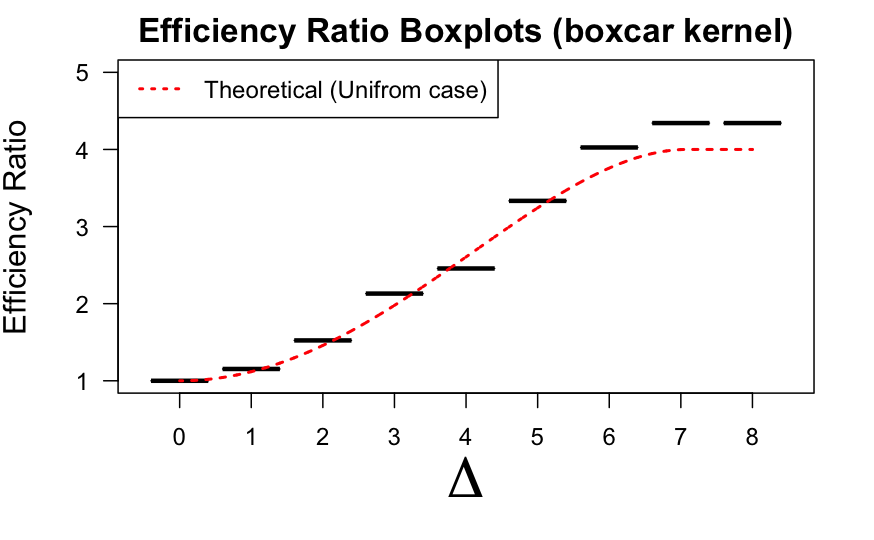
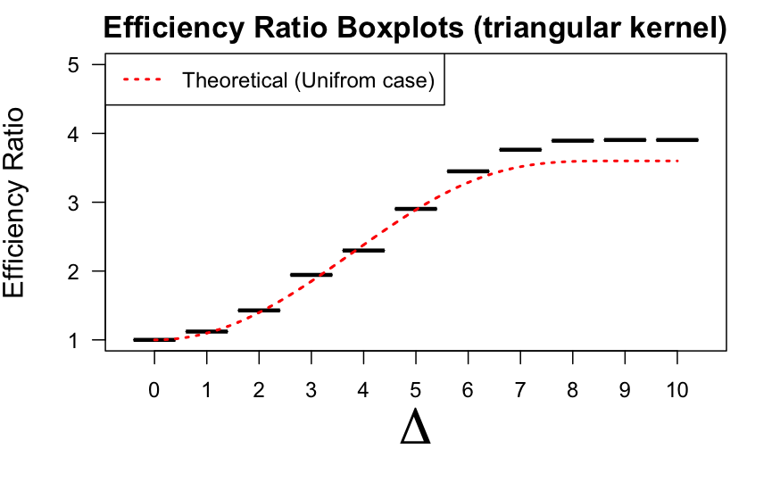
The second panel in Figure 2 shows versus the local experiment size . The efficiency curve has a similar monotone increasing shape as we saw for the boxcar kernel. The maximum efficiency ratio, at , is instead of . The efficiency ratio is a rational function of with a numerator of degree and a denominator of degree . It is strictly increasing on the interval , though the proof is lengthy enough to move to the Appendix.
Proposition 3.
The derivative of with respect to is positive for .
Proof.
See Appendix F. ∎


6 Classroom size data
We explored the efficiency ratio for the tie-breaker design for with a uniform distribution. While that can be arranged by using ranks, in other situations we might prefer to use the original value of a running variable and those might not be uniformly distributed. We show how to do this using a dataset from Angrist and Lavy 1999 on classroom sizes.
Angrist and Lavy 1999 studied the causal effect of classroom size on test performance of elementary school students in Israel. In Israel, the Maimonides rule mandates that elementary school classes cannot exceed 40 students. If a school has 41 students enrolled in a particular grade that grade must be split into two classes. Note that grades that have 40 or fewer enrolled students are allowed to split into multiple classes and that grades with slightly more than 40 students occasionally violate the Maimonides rule and do not split into multiple classes. Despite this, we can consider this a setting for RDD where the treatment variable is whether or not the school is legally mandated to split a particular grade into smaller classes.
The dataset, published on the Harvard Dataverse (Angrist and Lavy 2009), has verbal and math scores for 3rd, 4th and 5th graders across Israel. We chose to focus exclusively on 4th grade verbal scores as our response variable and 4th grade enrollments as our assignment variable because Angrist and Lavy 1999 suggest that a slightly significant effect of the treatment on 4th grade verbal scores exists. Even though the data were not generated by a tie-breaker we can still compute the relative efficiency that a tie-breaker design would have had.
To simplify the analysis, we removed all schools that either had more than 80 students or more than two 4th-grade classes from the dataset. We further removed all schools that had NA entries for either class size or verbal scores, leaving schools in our filtered dataset. See Figure 3 for a visualization of the distribution of the 4th grade enrollments and Figure 4 for visualizations of the local linear regression based-RDD on this dataset using boxcar and triangular kernels. We use the bandwidths given by the Imbens and Kalyanaraman 2012 procedure, which were computed using that paper’s MATLAB code. The apparent benefit from smaller classrooms is positive but small and it turns out, not statistically significant in this analysis. The 95% confidence interval (assuming homoscedastic errors) for the effect size at the boundary of the local linear regression-based RDD was when a boxcar kernel with bandwidth was used. The 95% confidence interval for the effect size at boundary of this RDD was when a triangular kernel with bandwidth was used.


Next we illustrate how an investigator can estimate the efficiency ratio of tie-breaker designs as a function of on sample values of the assignment variable. First we translate the data, replacing by to move the threshold from to . Next, for each of interest we use Monte Carlo samples to estimate and also , both up to a constant . That gives us efficiency ratios for each . In each of our samples, we simulate random assignments for a tie-breaker design at the given experimental radius . The random assignments are stratified: in each consecutive pair of classroom sizes in the experimental region, one was randomly chosen to have and the other got . The and the random let us compute the matrices and defined in the beginning of Section 5, from which we compute a non-asymptotic using (22). We do not simulate any values because efficiency only depends on , and we are retaining the bandwidths from the Imbens and Kalyanaraman 2012 procedure on the original data. A more detailed simulation randomizing the bandwidth choice is out of scope. Our simulations demonstrate that the TBD is more efficient at each fixed , so we expect that it will also be more efficient at a randomly chosen . There could be exceptions if the bandwidth is adversarially correlated with the estimation errors but we do not think that is likely.
Figure 5 shows boxplots of simulated values for various choices of to plot the full efficiency curve. It is clear from Figure 5 that with stratified allocations the efficiency is very reproducible. Figure 6 shows results for different bandwidths, ranging from to . Because the efficiencies are so reproducible given the bandwidth, we just plot curves of the mean and standard deviations of estimated values. For both the boxcar and triangular kernels, we see that the tie-breaker design is reproducibly more efficient than the RDD and the effect increases as increases for all we studied. The efficiency curves for this dataset under various bandwidth choices look similar to the theoretical efficiency curves derived in Section 5 for the case of a uniform assignment variable.


For a further discussion of the Maimonides rule, see Angrist et al. 2019. They consider different data sets and also investigate the possibility that the class sizes are sometimes manipulated to be above the threshold triggering a classroom split.
Comparison with theoretical results for uniform assignment variable
Our theoretical analysis in Section 5 is for a uniformly spaced assignment variable. We can offer one explanation for why the empirical efficiencies on non-uniformly distributed data look so similar to the theoretical ones for uniformly distributed data (see the left panels in Figure 6). The explanation uses some results about non-parametric regression from Fan and Gijbels 1996. Nonparametric regression estimates typically have an asymptotic variance where the leading term is proportional to where is the probability density of the . This arises because the local sample size is asymptotically proportional to . Hence, when considering nonuniform distributions, the factors in the leading order variance terms will cancel out when computing the efficiency ratios. Some of the nonparametric regression estimators, such as the Nadaraya-Watson estimator, have a lead term in their bias that depends on the derivative , and while for uniformly distributed data, it is not zero in general. Kernel weighted least squares methods (with symmetric ) do not have a dependency on in their bias. There is a curvature bias from but that is not related to the sampling distribution of the . The lead terms in bias and variance for local linear regressions do not distinguish between distributions with the same value of but different . Thus the effects of non-uniformity of are asymptotically negligible.
7 Discussion
If an investigator is able to implement a 3-level tie-breaker design with any experimental radius , our results show that the TBD has considerable statistical advantages over the RDD.
The most obvious advantage is that the TBD allows estimation of multiple causal parameters of interest including the average treatment effect over subjects with as well as the expected treatment effect at any particular . The former is estimable at a faster rate and with fewer assumptions, whereas the latter may still be of interest for choosing a future policy threshold. Meanwhile, the RDD only allows estimation of , the expected treatment effect at .
Even if the only goal is estimation of , our results indicate a statistical advantage to running a TBD rather than an RDD and an advantage to picking a larger experimental radius . As seen in Section 4, to achieve the same asymptotic MSE in mean squared optimal estimation of , a TBD would require roughly 64 percent fewer samples than would be needed for an RDD. Moreover, the asymptotic advantage for a TBD is largely driven by its lower variance (Figure 1). Hence, if the convenient, but controversial, method of undersmoothing to construct asymptotically valid confidence intervals for is used instead of more nearly optimal approaches, the TBD would exhibit even greater advantages over the RDD. We point readers to the introduction of Calonico, Cattaneo and Farrell 2018 for an overview of the history of undersmoothing, and Calonico, Cattaneo and Farrell 2019 for a modern approach to constructing confidence intervals that has better coverage properties than undersmoothing has.
In terms of the statistical advantages of picking a larger , Owen and Varian 2020 found an efficiency advantage for the tie-breaker in a global regression, wherein the estimation variance decreased monotonically in . We provide a comparable finding for the now more standard local linear regression approach: for any fixed bandwidth , we see a theoretical efficiency that increases with the amount of experimentation. We have not investigated the effect of on the subsequent choice of when , although one candidate choice is an that removes the leading order bias term, which we derived in Appendix D.
There is room for an improved estimator of in the TBD context which uses data from both treatments on both sides of the threshold . We leave this for further work. A critical ingredient is the estimation of . Compared to the method in Imbens and Kalyanaraman 2012, one could use a bandwidth tuned for an internal point instead of one tuned for an endpoint. Also the curvature estimates in Imbens and Kalyanaraman 2012 use local quadratic regressions while Fan and Gijbels 1996 suggest using local cubic regressions for curvature estimation at an interior point.
References
- Abdulkadiroğlu et al. (2022) [author] Abdulkadiroğlu, Atı̇laA., Angrist, Joshua DJ. D., Narita, YusukeY. and Pathak, ParagP. (2022). Breaking ties: Regression discontinuity design meets market design. Econometrica 90 117–151.
- Angrist, Autor and Pallais (2020) [author] Angrist, JoshuaJ., Autor, DavidD. and Pallais, AmandaA. (2020). MARGINAL EFFECTS OF MERIT AID FOR LOW-INCOME STUDENTS Technical Report, National Bureau of Economic Research.
- Angrist and Lavy (1999) [author] Angrist, Joshua DJ. D. and Lavy, VictorV. (1999). Using Maimonides’ rule to estimate the effect of class size on scholastic achievement. The Quarterly Journal of Economics 114 533–575.
- Angrist and Lavy (2009) [author] Angrist, Joshua D.J. D. and Lavy, VictorV. (2009). Replication data for: Using Maimonides’ Rule to Estimate the Effect of Class Size on Student Achievement. 10.7910/DVN/XRSUJU
- Angrist et al. (2019) [author] Angrist, Joshua DJ. D., Lavy, VictorV., Leder-Luis, JetsonJ. and Shany, AdiA. (2019). Maimonides’ Rule Redux. American Economic Review: Insights 1 309–24.
- Borchers (2019) Borchers, H. W. (2019). pracma: Practical Numerical Math Functions R package version 2.2.9.
- Boruch (1975) [author] Boruch, Robert FR. F. (1975). Coupling randomized experiments and approximations to experiments in social program evaluation. Sociological Methods & Research 4 31–53.
- Calonico, Cattaneo and Titiunik (2014) [author] Calonico, SebastianS., Cattaneo, Matias DM. D. and Titiunik, RocioR. (2014). Robust nonparametric confidence intervals for regression-discontinuity designs. Econometrica 82 2295–2326.
- Calonico, Cattaneo and Farrell (2018) [author] Calonico, SebastianS., Cattaneo, Matias D.M. D. and Farrell, Max H.M. H. (2018). On the Effect of Bias Estimation on Coverage Accuracy in Nonparametric Inference. Journal of the American Statistical Association 113 767-779. 10.1080/01621459.2017.1285776
- Calonico, Cattaneo and Farrell (2019) [author] Calonico, SebastianS., Cattaneo, Matias DM. D. and Farrell, Max HM. H. (2019). Optimal bandwidth choice for robust bias-corrected inference in regression discontinuity designs. The Econometrics Journal 23 192-210.
- Campbell (1969) [author] Campbell, Donald TD. T. (1969). Reforms as experiments. American psychologist 24 409.
- Cappelleri, Darlington and Trochim (1994) [author] Cappelleri, Joseph C.J. C., Darlington, Richard B.R. B. and Trochim, William M. K.W. M. K. (1994). Power Analysis of Cutoff-Based Randomized Clinical Trials. Evaluation Review 18 141-152. 10.1177/0193841X9401800202
- Cappelleri and Trochim (2003) [author] Cappelleri, Joseph C.J. C. and Trochim, William M. K.W. M. K. (2003). Cutoff Designs. In Encyclopedia of Biopharmaceutical Statistics (MarcelM. Dekker, ed.) CRC Press. 10.1081/E-EBS 12000734
- Cattaneo, Frandsen and Titiunik (2015) [author] Cattaneo, Matias DM. D., Frandsen, Brigham RB. R. and Titiunik, RocioR. (2015). Randomization inference in the regression discontinuity design: An application to party advantages in the US Senate. Journal of Causal Inference 3 1–24.
- Cattaneo and Titiunik (2022) [author] Cattaneo, Matias DM. D. and Titiunik, RocioR. (2022). Regression discontinuity designs. Annual Review of Economics 14 821–851.
- Cheng, Fan and Marron (1997) [author] Cheng, Ming-YenM.-Y., Fan, JianqingJ. and Marron, James SJ. S. (1997). On automatic boundary corrections. The Annals of Statistics 25 1691–1708.
- Crump et al. (2009) [author] Crump, Richard KR. K., Hotz, V JosephV. J., Imbens, Guido WG. W. and Mitnik, Oscar AO. A. (2009). Dealing with limited overlap in estimation of average treatment effects. Biometrika 96 187–199.
- Eckles et al. (2020) [author] Eckles, DeanD., Ignatiadis, NikolaosN., Wager, StefanS. and Wu, HanH. (2020). Noise-induced randomization in regression discontinuity designs Technical Report, arXiv:2004.09458.
- Fan and Gijbels (1996) [author] Fan, JianqingJ. and Gijbels, IreneI. (1996). Local polynomial modelling and its applications: monographs on statistics and applied probability 66 66. CRC Press, Boca Raton, FL.
- Gelman and Imbens (2019) [author] Gelman, AndrewA. and Imbens, GuidoG. (2019). Why High-Order Polynomials Should Not Be Used in Regression Discontinuity Designs. Journal of Business & Economic Statistics 37 447–456. 10.1080/07350015.2017.1366909
- Goldberger (1972) [author] Goldberger, A. S.A. S. (1972). Selection Bias in Evaluating Treatment Effects: Some Formal Illustrations Technical Report No. Discussion paper 128–72, Institute for Research on Poverty, University of Wisconsin–Madison.
- Hahn, Todd and der Klaauw (2001) [author] Hahn, JinyongJ., Todd, PetraP. and der Klaauw, Wilbert VanW. V. (2001). Identification and estimation of treatment effects with a regression-discontinuity design. Econometrica 69 201–209.
- Higham (2002) [author] Higham, Nicholas J.N. J. (2002). Accuracy and Stability of Numerical Algorithms, Second ed. Society for Industrial and Applied Mathematics, Philadelphia.
- Imbens and Kalyanaraman (2012) [author] Imbens, GuidoG. and Kalyanaraman, KarthikK. (2012). Optimal bandwidth choice for the regression discontinuity estimator. The Review of Economic Studies 79 933–959.
- Jacob et al. (2012) [author] Jacob, RobinR., Zhu, PeiP., Somers, Marie-AndréeM.-A. and Bloom, HowardH. (2012). A Practical Guide to Regression Discontinuity. MDRC.
- Krantz (2022) [author] Krantz, CassidyC. (2022). Modeling the outcomes of a longitudinal tie-breaker regression discontinuity design to assess an in-home training program for families at risk of child abuse and neglect, PhD thesis, University of Oklahoma.
- Li and Owen (2022) [author] Li, Harrison H.H. H. and Owen, Art B.A. B. (2022). A general characterization of optimal tie-breaker designs Technical Report No. arXiv:2202.12511, Stanford University.
- Metelkina and Pronzato (2017) [author] Metelkina, AsyaA. and Pronzato, LucL. (2017). Information-regret compromise in covariate-adaptive treatment allocation. The Annals of Statistics 45 2046–2073.
- Morrison and Owen (2022) [author] Morrison, Tim P.T. P. and Owen, Art B.A. B. (2022). Optimality in Multivariate Tie-breaker Designs Technical Report No. arXiv:2202.10030, Stanford University.
- Owen and Varian (2020) [author] Owen, A. B.A. B. and Varian, H.H. (2020). Optimizing the tie-breaker regression discontinuity design. Electronic Journal of Statistics 14 4004–4027.
- Rosenman and Rajkumar (2019) [author] Rosenman, EvanE. and Rajkumar, KarthikK. (2019). Optimized Partial Identification Bounds for Regression Discontinuity Designs with Manipulation Technical Report No. arXiv:1910.02170, Stanford University.
- Thistlethwaite and Campbell (1960) [author] Thistlethwaite, D. L.D. L. and Campbell, D. T.D. T. (1960). Regression-discontinuity analysis: An alternative to the ex post facto experiment. Journal of Educational psychology 51 309.
- Wand and Jones (1994) [author] Wand, Matt PM. P. and Jones, M ChrisM. C. (1994). Kernel smoothing. Chapman Hall/CRC, Boca Raton, FL.
A Proof of Lemma 2
Without loss of generality suppose (if this is not the case we can define a new assignment variable to be a translation of the original assignment variable by ). It is convenient to define
Also define . Letting , define
for nonnegative integers .
Next, let be the conditional density of given that . That is
| (34) |
We now prove some helpful small bandwidth approximations for and .
Lemma A.1.
Proof.
We will prove this for and the proof for will be identical. First note that is the average of IID random variables so
Now note that
where the last equality holds because is bounded with bounded support, is continuously differentiable at , and asymptotically .
Meanwhile, the term is upper bounded by
where the last equality holds because is bounded with bounded support, is continuous and strictly positive at , and asymptotically . Thus
where last equality holds because as , , so , and because .
Combining previous results
Lemma A.2.
Proof.
We will prove this for and the proof for will be identical. First note that is the average of IID random variables so
Now note that equals
| (35) |
where the last equality holds because is bounded with bounded support, is continuous at , and asymptotically .
Meanwhile, the term is upper bounded by
where the last equality holds because is bounded with bounded support, is continuous and strictly positive at , and asymptotically .
Thus
where the last equality holds because as , , so , and because . Combining previous results,
We are now ready to compute an asymptotic approximation for the bias and variance of the causal estimator . Recall that as discussed in Section 3, can be equivalently estimated by solving two separate local linear regressions, one for the treatment group and one for the control group, rather than solving (4) and plugging the solution into (5). In this proof, we use the two separate local linear regression formulation, so that the proof more closely resembles that seen in the appendix of Imbens and Kalyanaraman 2012.
In particular, define and to be the design matrices for the local linear regression restricted to the treated group and the control group respectively. That is define
Also define the corresponding local linear regression weight matrices by
and similarly define the corresponding conditional variance matrices by
Finally, define , , and let . The causal estimator for is given by , where and are the local linear regression estimators given by
Let be the full design matrix whose ith row is , and note that the matrices and and the sets and are functions of the full design matrix.
In the next subsection, we compute the asymptotic approximation to the bias of the estimator , and in the following subsection, we compute the asymptotic approximation to its variance . These calculations leverage Lemmas A.1 and A.2.
Asymptotic approximation of the bias
Define and , and note that
We will compute the asymptotic formula for , and by an identical argument, the asymptotic formula for will follow.
To do this note that
where .
Since has at least three continuous derivatives in an open neighborhood of , for each ,
where .
So letting and it follows that
Combining previous results
Since (by the Cauchy-Schwartz inequality), Lemma A.1 and a first order Taylor expansion, as and , yield
Hence, by Lemma A.1 again,
Now note, that since is continuous in an open neighborhood of , there exists an for which . Since has bounded support, there exists an such that for all , whenever . Therefore for all and all ,
Thus for all sufficiently small,
where the bottom equality holds by Lemma A.1, and the top equality holds by the exact same argument as the proof of Lemma A.1 except with absolute values.
Combining the two previous results and multiplying through and dividing by ,
Similarly, by Lemma A.1,
and therefore,
A similar argument shows that
Hence, recalling that the bias is given by it follows that the asymptotic formula for the bias is
| (36) |
Squaring the above formula, we recover the leading order squared-bias. As noted in Section 4, the leading order squared-bias is the first term in (12).
Asymptotic approximation of the variance
Defining , the variance for our causal estimator is
where the last equality holds because are IID by assumption making and independent conditionally on the treatment assignments which then implies that are independent conditionally on .
We now compute an asymptotic formula for and by an identical argument, the asymptotic formula for will follow.
First note that
Now the middle factor rescaled by is
and recall from the previous subsection that
Thus,
Thus dividing through by and rearranging terms,
Asymptotic expression for mean squared error
Asymptotically optimal bandwidth expression
Because by assumption and , a simple calculus exercise shows that
B Proof of Theorem 1
C Extensions to assignment probability
In this appendix we consider the MSE of a generalization of the 3-level TBD given by (1), where we allow the assignment probabilities to and to differ from within the interval of experimentation. In particular, we consider a design with the following assignment probabilities
| (38) |
for some . Under this more general version of the TBD, one can show that the AMSE formula given in (12) changes to
| (39) |
and that the following lemma holds.
Lemma C.1.
Proof.
Analogously to the empirical bandwidth choice given by (18), an investigator running a TBD of the form (38) seeking mean squared optimal estimation of would ultimately use the bandwidth
where is some consistent estimator of the quantity
To derive an analogue of Theorem 1 for a TBD of the form (38), it is convenient to define the relative variance measure
| (41) |
The following theorem compares the RDD with points to a TBD of the form (38) with points for some .
Theorem C.1.
Proof.
We visualize the implications of Theorem C.1 in Figure C.1. While the figure focuses on the case of the triangular kernel with , the relative AMSE as a function of and will be a scalar multiple of that shown in Figure C.1 for different kernels and values of . We also explicitly list a few notable implications of Theorem C.1 below.

- 1.
The AMSE for the TBD is minimized by .
- 2.
If either or , then
As a result, whenever is between and inclusive, the advantage of a TBD over an RDD (in terms of relative asymptotic MSE in estimation of ) is at least as large as that described in Table 1, which corresponds to the case.
- 3.
Suppose that a TBD and RDD are to be conducted with the same sample size (i.e. ), and that under both designs the asymptotically MSE optimal bandwidth is to be used. Then, regardless of the unknown value of , for any choice of with defined at (20), the TBD given by (38) will have lower AMSE than the RDD. Conversely, if , there will exist a range of values of contained in for which the TBD will have higher AMSE than the RDD. Note that amongst the common kernel choices considered in Table 1, is largest for the triangular kernel with a value of precisely , suggesting that for any of these kernel choices the TBD will have lower AMSE than an RDD in estimating as long as , but outside that range, the TBD may have larger AMSE depending on the kernel choice and the unknown value of .
The first fact may be difficult to leverage in practice because at the time an experiment is being designed, the investigator is unlikely to have outcome data from both treatment and control units that they can use to estimate the ratio . If the investigator has some prior knowledge about whether or not is smaller or greater than 1, they could potentially leverage the second fact to design a TBD that has lower AMSE than a TBD with the default of has. The third statement is true for any value of or , suggesting that a design with should only be considered with caution.
D Bandwidth that removes leading order bias
In the asymptotic analysis from Section 4, the bias for the local linear estimator of was . However, that analysis relied on a simplification that arose by assuming that as . In this appendix, we derive an asymptotic expression for the bias of that does not rely on the assumption that as . In this expression for the bias, the leading order term is quadratic in . We also show that for some value of , which depends only on the kernel , the quadratic bias term vanishes. In Table D.1, we present a numerical approximation of the value of that removes the leading order bias for common kernel choices.
We consider the following regularity conditions, which were not needed in the main text.
- (I)
The mean functions are three times differentiable. Further, the third derivatives of the mean functions, , are bounded.
- (II)
The density of the assignment variable satisfies for some .
In the proof of Lemma 2, where we computed the leading order bias, we did not need to assume (I) and (II) because we supposed that as . In the following theorem about the leading order bias, because we do not assume , we assume (I) and (II) in addition to (i)–(vi).
Theorem D.1.
Suppose conditions (i)–(vi) from the main text and conditions (I) and (II) hold, and that . Let be fixed. Under the tie-breaker design defined by (1) and estimation of according to (4) and (5) for some bandwidth , the bias of is given by
| (43) |
where is defined at (10). As a result, the leading order bias term is equal to whenever the bandwidth is chosen so that
| (44) |
Moreover, there must exist an that satisfies (44).
Proof.
Fix and suppose without loss of generality that . Define , , , for , , ,, , , and , according to the same definitions presented in Appendix A.
We will first derive a formula for that is similar to that given in Lemma A.1, except here we will not rely on a simplification that occurs in the asymptotic regime where , eventually dropping below .
For any nonnegative integer , because the samples are IID, we get
To simplify this expression further, observe that, for any and nonnegative integer ,
where above the last two steps hold by Assumptions (II) and (iv) respectively, and as a consequence, for any ,
Combining this with the above formula for ,
where
If we define a similar argument yields an analogous formula for , and hence
| (45) |
By noting the similarities between the formula for in Lemma A.1 and that from (45), the formula for can be derived by the same argument presented in Appendix A, by simply replacing terms with , terms with terms, and intermediary terms with , for any integer . Because we now no longer assume as , there are three steps where we have to use a slightly different argument from that presented in Appendix A. First, since we no longer assume that , the 2nd order Taylor expansion of the mean functions with the remainder terms require that is continuous everywhere, rather than merely in a neighborhood of which is given by Assumption (iii). Assumption (I) that is bounded, guarantees that is continuous everywhere because differentiability implies continuity. Second, we can use Assumption (I) that is bounded to show that there exists an for which for any . In Appendix A, we did not need Assumption (I) since we supposed that , so it was enough to show that inequality holds for any sufficiently small . Third, the argument involves a first order Taylor expansion of the quantity . In the current setting where we do not suppose as , we must now ascertain that with probability approaching as , is positive and bounded away from zero. Recalling that up to an term, , equals , by the Cauchy-Schwartz inequality it follows that
Hence with probability converging to as , is positive and bounded away from zero. Consequently, the following first order Taylor expansion holds for all
where the denominator in the first term is positive and bounded away from by a similar Cauchy-Schwartz argument that leverages symmetry of .
By the same derivation of the bias formula presented in Appendix A, with the exceptions in the argument noted above, the bias of is given by
A similar argument shows that,
Now note that the bias of is given by . To simplify the expression for , observe that by symmetry of , for any
The above is defined at (10). Hence, subtracting from the bias for is given by
Since we supposed without loss of generality, this proves (43).
Now, since is bounded away from zero, the leading order term in in formula (43) for the bias of is zero whenever satisfies (44).
To prove the final claim, that there exists an solving (44), define
Clearly by boundedness and continuity of , is continuous on . Recalling Assumption (iv) that is supported on , . Since , . Also note that by symmetry of the kernel and the Cauchy-Schwartz inequality,
Since , and since is continuous on , there must exist some with . Clearly this satisfies equation (44) and . ∎
| Kernel | Function | Support | Bandwidth solving (44) |
|---|---|---|---|
| Boxcar | |||
| Triangular | |||
| Epanechnikov | |||
| Quartic | |||
| Triweight | |||
| Tricube | |||
| Cosine |
E Proof of Proposition 2
Note that for the triangular kernel, and . By substituting these expressions into formula (30) for the efficiency ratio and cancelling out a common factor of from the numerator and denominator, it follows that
F Proof of Proposition 3
We want to show that this function
has a positive derivative for . The numerator has degree and the denominator has degree . The customary formula for the derivative of a rational function produces a rational function with a non-negative denominator and a numerator of degree . We will work through a sequence of steps reducing the degree of this polynomial to show that the numerator must be positive on . That then rigorously establishes the monotonicity of which is visually apparent.
It is convenient to work instead with . Then and Therefore where is a function given by
for and having replaced by we will show that .
In the usual formula for the derivative of a ratio, has this numerator
Notice that for and so . As a result, the sign of is preserved by dividing it by , yielding
Now since and and we can divide by finding that it has the same sign as
We can divide by getting a polynomial with the opposite sign from . This yields
Note that the coefficient of in is a zero that must not be left out when entering the coefficients into symbolic differentiation codes.
We want to show that for which then makes and ultimately so that for .
Our next step is to show that for all . Note that
Graphing versus and evaluating it numerically, makes it is clear that . Our next few steps are just to eliminate even an unreasonable doubt about the sign of . Some readers might prefer to skip that and go instead to the subsection marked “Conclusion of the proof”.
Positivity of
We begin by writing
Then by the triangle inequality,
| (47) |
for all .
Now for define . For each we will let be the numerical evaluation for the polynomial computed using Horner’s method with double-precision in R, implemented with the ‘horner’ function in the pracma R package of Borchers 2019.
By formula (5.3) in Higham 2002, the absolute error in Horner’s method for the polynomial is at most where , is the unit roundoff, and .
Applying that bound to our 6th degree polynomial , and noting that for each , will be at most the sum of the absolute value of the coefficients we find that
| (48) |
We need not worry about floating point error induced by evaluating , because each is a floating point number. For double precision in R, the unit roundoff is from which , and so the maximum error in (48) is at most . The smallest value of among all evaluation points was and so .
Now we are ready to prove that for all . For any there exists with . By (47) we know that is Lipschitz continuous on with Lipschitz constant . Therefore
holds for all
Conclusion of the proof
We have shown above that for any . Now since , and for all , it follows that for all . Finally since and for all , it follows that for all . This completes the proof. ∎