Machine learning of high dimensional data on a noisy quantum processor Preprint: FERMILAB-PUB-20-624-QIS
Abstract
We present a quantum kernel method for high-dimensional data analysis using Google’s universal quantum processor, Sycamore. This method is successfully applied to the cosmological benchmark of supernova classification using real spectral features with no dimensionality reduction and without vanishing kernel elements. Instead of using a synthetic dataset of low dimension or pre-processing the data with a classical machine learning algorithm to reduce the data dimension, this experiment demonstrates that machine learning with real, high dimensional data is possible using a quantum processor; but it requires careful attention to shot statistics and mean kernel element size when constructing a circuit ansatz. Our experiment utilizes 17 qubits to classify 67 dimensional data - significantly higher dimensionality than the largest prior quantum kernel experiments - resulting in classification accuracy that is competitive with noiseless simulation and comparable classical techniques.
Keywords:
quantum computing, machine learning, kernel methodsI Introduction
Quantum kernel methods (QKM) Havlícek et al. 2019; Schuld and Killoran 2019 provide techniques for utilizing a quantum co-processor in a machine learning setting. These methods were recently proven to provide a speedup over classical methods for certain specific input data classes Liu et al. 2020. They have also been used to quantify the computational power of data in quantum machine learning algorithms and drive the conditions under which quantum models will be capable of outperforming classical ones Huang et al. 2020. Prior experimental work Kusumoto et al. 2019; Bartkiewicz et al. 2020; Havlícek et al. 2019 has focused on artificial or heavily pre-processed data, hardware implementations involving very few qubits, or circuit connectivity unsuitable for NISQ Preskill 2018 processors; recent experimental results show potential for many-qubit applications of QKM to high energy physics Wu et al. 2020.
In this work, we extend the method of machine learning based on quantum kernel methods up to 17 hardware qubits requiring only nearest-neighbor connectivity. We use this circuit structure to prepare a kernel matrix for a classical support vector machine to learn patterns in 67-dimensional supernova data for which competitive classical classifiers fail to achieve 100% accuracy. To extract useful information from a processor without quantum error correction (QEC), we implement error mitigation techniques specific to the QKM algorithm and experimentally demonstrate the algorithm’s robustness to some of the device noise. Additionally, we justify our circuit design based on its ability to produce large kernel magnitudes that can be sampled to high statistical certainty with relatively short experimental runs.
We implement this algorithm on the Google Sycamore processor which we accessed through Google’s Quantum Computing Service. This machine is similar to the quantum supremacy demonstration Sycamore chip Arute et al. 2019, but with only 23 qubits active. We achieve competitive results on a nontrivial classical dataset, and find intriguing classifier robustness in the face of moderate circuit fidelity. Our results motivate further theoretical work on noisy kernel methods and on techniques for operating on real, high-dimensional data without additional classical pre-processing or dimensionality reduction.
II Quantum kernel Support Vector Machines
A common task in machine learning is supervised learning, wherein an algorithm consumes datum-label pairs and outputs a function that ideally predicts labels for seen (training) input data and generalizes well to unseen (test) data. A popular supervised learning algorithm is the Support Vector Machine (SVM) Cortes and Vapnik 1995; Boser et al. 1992 which is trained on inner products in the input space to find a robust linear classification boundary that best separates the data. An important technique for generalizing SVM classifiers to non-linearly separable data is the so-called “kernel trick” which replaces in the SVM formulation by a symmetric positive definite kernel function Aizerman et al. 1964. Since every kernel function corresponds to an inner product on input data mapped into a feature Hilbert space Aronszajn 1950, linear classification boundaries found by an SVM trained on a high-dimensional mapping correspond to complex, non-linear functions in the input space.

Quantum kernel methods can potentially improve the performance of classifiers by using a quantum computer to map input data in into a high-dimensional complex Hilbert space, potentially resulting in a kernel function that is expressive and challenging to compute classically. It is difficult to know without sophisticated knowledge of the data generation process whether a given kernel is particularly suited to a dataset, but perhaps families of classically hard kernels may be shown empirically to offer performance improvements. In this work we focus on a non-variational quantum kernel method, which uses a quantum circuit to map real data into quantum state space according to a map . The kernel function we employ is then the squared inner product between pairs of mapped input data given by , which allows for more expressive models compared to the alternative choice Huang et al. 2020.
In the absence of noise, the kernel matrix for a fixed dataset can therefore be estimated up to statistical error by using a quantum computer to sample outputs of the circuit and then computing the empirical probability of the all-zeros bitstring. However in practice, the kernel matrix sampled from the quantum computer may be significantly different from due to device noise and readout error. Once is computed for all pairs of input data in the training set, a classical SVM can be trained on the outputs of the quantum computer. An SVM trained on a size- training set learns to predict the class of an input data point according to the decision function:
| (1) |
where and are parameters determined during the training stage of the SVM. Training and evaluating the SVM on requires an kernel matrix, after which each data point in the testing set may be classified using an additional evaluations of for . Figure 1 provides a schematic representation of the process used to train an SVM using quantum kernels.
II.1 Data and preprocessing
We used the dataset provided in the Photometric LSST Astronomical Time-series Classification Challenge (PLAsTiCC) The PLAsTiCC team et al. 2018 that simulates observations of the Vera C. Rubin Observatory ver 2020. The PLAsTiCC data consists of simulated astronomical time series for several different classes of astronomical objects. The time series consist of measurements of flux at six wavelength bands. Here we work on data from the training set of the challenge. To transform the problem into a binary classification problem, we focus on the two most represented classes, 42 and 90, which correspond to types II and Ia supernovae, respectively.
Each time series can have a different number of flux measurements in each of the six wavelength bands. In order to classify different time series using an algorithm with a fixed number of inputs, we transform each time series into the same set of derived quantities. These include: the number of measurements; the minimum, maximum, mean, median, standard deviation, and skew of both flux and flux error; the sum and skew of the ratio between flux and flux error, and of the flux times squared flux ratio; the mean and maximum time between measurements; spectroscopic and photometric redshifts for the host galaxy; the position of each object in the sky; and the first two Fourier coefficients for each band, as well as kurtosis and skewness. In total, this transformation yields a 67-dimensional vector for each object.
To prepare data for the quantum circuit, we convert lognormal-distributed spectral inputs to scale, and normalize all inputs to . We perform no dimensionality reduction. Our data processing pipeline is consistent with the treatment applied to state-of-the-art classical methods. Our classical benchmark is a competitive solution to this problem, although significant additional feature engineering leveraging astrophysics domain knowledge could possibly raise the benchmark score by a few percent.
II.2 Circuit design
To compute the kernel matrix over the fixed dataset we must run repetitions of each circuit to determine the total counts of the all zeros bitstring, resulting in an estimator . This introduces a challenge since quantum kernels must also be sampled from hardware with low enough statistical uncertainty to recover a classifier with similar performance to noiseless conditions. Since the likelihood of large relative statistical error between and grows with decreasing magnitude of and decreasing , the performance of the hardware-based classifier will degrade when the kernel matrix to be sampled is populated by small entries. Conversely, large kernel magnitudes are a desirable feature for a successful quantum kernel classifier, and a key goal in circuit design is to balance the requirement of large kernel matrix elements with a choice of mapping that is difficult to compute classically. Another significant design challenge is to construct a circuit that separates data according to class without mapping data so far apart as to lose information about class relationships - an effect sometimes referred to as the “curse of dimensionality” in classical machine learning.
For this experiment, we accounted for these design challenges and the need to accommodate high-dimensional data by mapping data into quantum state space using the quantum circuit shown in Figure 2. Each local rotation in the circuit is parameterized by a single element of preprocessed input data so that inner products in the quantum state space correspond to a similarity measure for features in the input space. Importantly, the circuit structure is constrained by matching the input data dimensionality to the number of local rotations so that the circuit depth and qubit count individually do not significantly impact the performance of the SVM classifier in a noiseless setting. This circuit structure consistently results in large magnitude inner products (median ) resulting in estimates for with very little statistical error. We provide further empirical evidence justifying our choice of circuit in Appendix B.
III Hardware classification results
III.1 Dataset selection
We are motivated to minimize the size since the complexity cost of training an SVM on datapoints scales as . However too small a training sample will result in poor generalization of the trained model, resulting in low quality class predictions for data in the reserved size- test set . We explored this tradeoff by simulating the classifiers for varying train set sizes in Cirq team and collaborators 2020 to construct learning curves (Figure 3) standard in machine learning. We found that our simulated 17-qubit classifier applied to 67-dimensional supernova data was competitive compared to a classical SVM trained using the Radial Basis Function (RBF) kernel on identical data subsets. For hardware runs, we constructed train/test datasets for which the mean train and k-fold validation scores achieved approximately the mean performance over randomly downsampled data subsets, accounting for the SVM hyperparameter optimization. The final dataset for each choice of qubits was constructed by producing a simulated kernel matrix , repeatedly performing 4-fold cross validation on a size-280 subset, and then selecting as the train/test set the exact elements from the fold that resulted in an accuracy closest to the mean validation score over all trials and folds.
III.2 Hardware classification and Postprocessing
We computed the quantum kernels experimentally using the Google Sycamore processor Arute et al. 2019 accessed through Google’s Quantum Computing Service. At the time of experiments, the device consisted of 23 superconducting qubits with nearest neighbor (grid) connectivity. The processor supports single-qubit Pauli gates with randomized benchmarking fidelity and native entangling gates with XEB fidelities Neill et al. 2018; Arute et al. 2019 typically greater than .
To test our classifier performance on hardware, we trained a quantum kernel SVM using qubit circuits for on supernova data with balanced class priors using a train/test split. We ran 5000 repetitions per circuit for a total of experiments per number of qubits. As described in Section III.1, the train and test sets were constructed to provide a faithful representation of classifier accuracy applied to datasets of restricted size. Typically the time cost of computing the decision function (Equation 1) is reduced to some fraction of since only a small subset of training inputs are selected as support vectors. However in hardware experiments we observed that a large fraction () of data in were selected as support vectors, likely due to a combination of a complex decision boundary and noise in the calculation of .
Training the SVM classifier in postprocessing required choosing a single hyperparameter that applies a penalty for misclassification, which can significantly affect the noise robustness of the final classifier. To determine without overfitting the model, we performed leave-one-out cross validation (LOOCV) on to determine corresponding to the maximum mean LOOCV score. We then fixed to evaluate the test accuracy on reserved datapoints taken from . Figure 4 shows the classifier accuracies for each number of qubits, and demonstrates that the performance of the QKM is not restricted by the number of qubits used. Significantly, the QKM classifier performs reasonably well even when observed bitstring probabilities (and therefore ) are suppressed by a factor of 50%-70% due to limited circuit fidelity. This is due in part to the fact that the SVM decision function is invariant under scaling transformations and highlights the noise robustness of quantum kernel methods.
IV Conclusion and outlook
Whether and how quantum computing will contribute to machine learning for real world classical datasets remains to be seen. In this work, we have demonstrated that quantum machine learning at an intermediate scale (10 to 17 qubits) can work on “natural” datasets using Google’s superconducting quantum computer. In particular, we presented a novel circuit ansatz capable of processing high-dimensional data from a real-world scientific experiment without dimensionality reduction or significant pre-processing on input data, and without the requirement that the number of qubits matches the data dimensionality. We demonstrated classification results that were competitive with noiseless simulation despite hardware noise and lack of quantum error correction. While the circuits we implemented are not candidates for demonstrating quantum advantage, these findings suggest quantum kernel methods may be capable of achieving high classification accuracy on near-term devices.
Careful attention must be paid to the impact of shot statistics and kernel element magnitudes when evaluating the performance of quantum kernel methods. This work highlights the need for further theoretical investigation under these constraints, as well as motivates further studies in the properties of noisy kernels.
The main open problem is to identify a “natural” data set that could lead to beyond-classical performance for quantum machine learning. We believe that this can be achieved on datasets that demonstrate correlations that are inherently difficult to represent or store on a classical computer, hence inherently difficult or inefficient to learn/infer on a classical computer. This could include quantum data from simulations of quantum many-body systems near a critical point or solving linear and nonlinear systems of equations on a quantum computer Kiani et al. 2020; Lloyd et al. 2020. The quantum data could be also generated from quantum sensing and quantum communication applications. The software library TensorFlow Quantum (TFQ) Broughton et al. 2020 was recently developed to facilitate the exploration of various combinations of data, models, and algorithms for quantum machine learning. Very recently, a quantum advantage has been proposed for some engineered dataset and numerically validated on up to 30 qubits in TFQ using similar quantum kernel methods as described in this experimental demonstration Huang et al. 2020. These developments in quantum machine learning alongside the experimental results of this work suggest the exciting possibility for realizing quantum advantage with quantum machine learning on near term processors.
Acknowledgements.
We would like to thank Google Quantum AI team for time on their Sycamore-chip quantum computer. In particular, the presentation and discussion with Kostyantyn Kechedzhi on error mitigation techniques that was incorporated into this experiment and Ping Yeh’s participation in some of the group discussions. Pedram Roushan provided a great deal of useful feedback on early versions of the draft and joined in several useful discussions. We would also like to thank Stavros Efthymiou for some early work on the quantum circuit simulations, and Brian Nord for consultation on interesting datasets in the domain of astrophysics and cosmology. EP is partially supported through A Kempf’s Google Faculty Award. JC, GP, and EP are partially supported by the DOE/HEP QuantISED program grant HEP Machine Learning and Optimization Go Quantum, identification number 0000240323. This manuscript has been authored by Fermi Research Alliance, LLC under Contract No. DE-AC02-07CH11359 with the U.S. Department of Energy, Office of Science, Office of High Energy Physics.References
- Havlícek et al. (2019) V. Havlícek, A. D. Córcoles, K. Temme, A. W. Harrow, A. Kandala, J. M. Chow, and J. M. Gambetta, Supervised learning with quantum-enhanced feature spaces, Nature 567, 209 (2019).
- Schuld and Killoran (2019) M. Schuld and N. Killoran, Quantum machine learning in feature hilbert spaces, Phys. Rev. Lett. 122, 040504 (2019).
- Liu et al. (2020) Y. Liu, S. Arunachalam, and K. Temme, A rigorous and robust quantum speed-up in supervised machine learning (2020), arXiv:2010.02174 [quant-ph] .
- Huang et al. (2020) H.-Y. Huang, M. Broughton, M. Mohseni, R. Babbush, S. Boixo, H. Neven, and J. R. McClean, Power of data in quantum machine learning (2020), arXiv:2011.01938 [quant-ph] .
- Kusumoto et al. (2019) T. Kusumoto, K. Mitarai, K. Fujii, M. Kitagawa, and M. Negoro, Experimental quantum kernel machine learning with nuclear spins in a solid (2019), arXiv:1911.12021 [quant-ph] .
- Bartkiewicz et al. (2020) K. Bartkiewicz, C. Gneiting, A. Černoch, K. Jiráková, K. Lemr, and F. Nori, Experimental kernel-based quantum machine learning in finite feature space, Scientific Reports 10, 1 (2020).
- Preskill (2018) J. Preskill, Quantum Computing in the NISQ era and beyond, Quantum 2, 79 (2018).
- Wu et al. (2020) S. L. Wu, J. Chan, W. Guan, S. Sun, A. Wang, C. Zhou, M. Livny, F. Carminati, A. D. Meglio, A. C. Y. Li, J. Lykken, P. Spentzouris, S. Y.-C. Chen, S. Yoo, and T.-C. Wei, Application of quantum machine learning using the quantum variational classifier method to high energy physics analysis at the lhc on ibm quantum computer simulator and hardware with 10 qubits (2020), arXiv:2012.11560 [quant-ph] .
- Arute et al. (2019) F. Arute, K. Arya, R. Babbush, D. Bacon, J. C. Bardin, R. Barends, R. Biswas, S. Boixo, F. G. S. L. Brandao, D. A. Buell, B. Burkett, Y. Chen, Z. Chen, B. Chiaro, R. Collins, W. Courtney, A. Dunsworth, E. Farhi, B. Foxen, A. Fowler, C. Gidney, M. Giustina, R. Graff, K. Guerin, S. Habegger, M. P. Harrigan, M. J. Hartmann, A. Ho, M. Hoffmann, T. Huang, T. S. Humble, S. V. Isakov, E. Jeffrey, Z. Jiang, D. Kafri, K. Kechedzhi, J. Kelly, P. V. Klimov, S. Knysh, A. Korotkov, F. Kostritsa, D. Landhuis, M. Lindmark, E. Lucero, D. Lyakh, S. Mandrà, J. R. McClean, M. McEwen, A. Megrant, X. Mi, K. Michielsen, M. Mohseni, J. Mutus, O. Naaman, M. Neeley, C. Neill, M. Y. Niu, E. Ostby, A. Petukhov, J. C. Platt, C. Quintana, E. G. Rieffel, P. Roushan, N. C. Rubin, D. Sank, K. J. Satzinger, V. Smelyanskiy, K. J. Sung, M. D. Trevithick, A. Vainsencher, B. Villalonga, T. White, Z. J. Yao, P. Yeh, A. Zalcman, H. Neven, and J. M. Martinis, Quantum supremacy using a programmable superconducting processor, Nature 574, 505 (2019).
- Cortes and Vapnik (1995) C. Cortes and V. Vapnik, Support-vector networks, Machine learning 20, 273 (1995).
- Boser et al. (1992) B. E. Boser, I. M. Guyon, and V. N. Vapnik, A training algorithm for optimal margin classifiers, in Proceedings of the Fifth Annual Workshop on Computational Learning Theory, COLT ’92 (ACM, New York, NY, USA, 1992) pp. 144–152.
- Aizerman et al. (1964) M. Aizerman, E. Braverman, and R. Rozoner, Theoretical foundations of potential function method in pattern recognition learning, Automation and Remote Control 6, 821 (1964).
- Aronszajn (1950) N. Aronszajn, Theory of reproducing kernels, Transactions of the American mathematical society 68, 337 (1950).
- The PLAsTiCC team et al. (2018) The PLAsTiCC team, T. A. Jr., A. Bahmanyar, R. Biswas, M. Dai, L. Galbany, R. Hložek, E. E. O. Ishida, S. W. Jha, D. O. Jones, R. Kessler, M. Lochner, A. A. Mahabal, A. I. Malz, K. S. Mandel, J. R. Martínez-Galarza, J. D. McEwen, D. Muthukrishna, G. Narayan, H. Peiris, C. M. Peters, K. Ponder, C. N. Setzer, The LSST Dark Energy Science Collaboration, and The LSST Transients and Variable Stars Science Collaboration, The photometric lsst astronomical time-series classification challenge (plasticc): Data set (2018), arXiv:1810.00001 [astro-ph.IM] .
- ver (2020) Vera C. Rubin Observatory, https://www.lsst.org/about (2020).
- team and collaborators (2020) Q. A. team and collaborators, Cirq (2020).
- Neill et al. (2018) C. Neill, P. Roushan, K. Kechedzhi, S. Boixo, S. V. Isakov, V. Smelyanskiy, A. Megrant, B. Chiaro, A. Dunsworth, K. Arya, R. Barends, B. Burkett, Y. Chen, Z. Chen, A. Fowler, B. Foxen, M. Giustina, R. Graff, E. Jeffrey, T. Huang, J. Kelly, P. Klimov, E. Lucero, J. Mutus, M. Neeley, C. Quintana, D. Sank, A. Vainsencher, J. Wenner, T. C. White, H. Neven, and J. M. Martinis, A blueprint for demonstrating quantum supremacy with superconducting qubits, Science 360, 195 (2018), https://science.sciencemag.org/content/360/6385/195.full.pdf .
- Kiani et al. (2020) B. T. Kiani, G. D. Palma, D. Englund, W. Kaminsky, M. Marvian, and S. Lloyd, Quantum advantage for differential equation analysis (2020), arXiv:2010.15776 [quant-ph] .
- Lloyd et al. (2020) S. Lloyd, G. D. Palma, C. Gokler, B. Kiani, Z.-W. Liu, M. Marvian, F. Tennie, and T. Palmer, Quantum algorithm for nonlinear differential equations (2020), arXiv:2011.06571 [quant-ph] .
- Broughton et al. (2020) M. Broughton, G. Verdon, T. McCourt, A. J. Martinez, J. H. Yoo, S. V. Isakov, P. Massey, M. Y. Niu, R. Halavati, E. Peters, M. Leib, A. Skolik, M. Streif, D. V. Dollen, J. R. McClean, S. Boixo, D. Bacon, A. K. Ho, H. Neven, and M. Mohseni, Tensorflow quantum: A software framework for quantum machine learning (2020), arXiv:2003.02989 [quant-ph] .
- Burges (1998) C. J. Burges, A tutorial on support vector machines for pattern recognition, Data mining and knowledge discovery 2, 121 (1998).
- Shawe-Taylor et al. (2004) J. Shawe-Taylor, N. Cristianini, et al., Kernel methods for pattern analysis (Cambridge university press, 2004).
- Fletcher (1987) R. Fletcher, Practical Methods of Optimization., Vol. 2 (John Wiley and Sons, Inc., 1987).
- Kuhn and Tucker (1951) H. W. Kuhn and A. W. Tucker, Nonlinear programming, in Proceedings of the Second Berkeley Symposium on Mathematical Statistics and Probability (University of California Press, Berkeley, Calif., 1951) pp. 481–492.
- Goemans (2015) M. Goemans, Lecture notes in 18.310a principles of discrete applied mathematics (2015).
- Farhi and Neven (2018) E. Farhi and H. Neven, Classification with quantum neural networks on near term processors (2018), arXiv preprint arXiv:1802.06002 (2018).
- F.R.S. (1901) K. P. F.R.S., Liii. on lines and planes of closest fit to systems of points in space, The London, Edinburgh, and Dublin Philosophical Magazine and Journal of Science 2, 559 (1901), https://doi.org/10.1080/14786440109462720 .
- Tilma and Sudarshan (2004) T. Tilma and E. Sudarshan, Generalized euler angle parameterization for u(n) with applications to su(n) coset volume measures, Journal of Geometry and Physics 52, 263 (2004).
- Kandala et al. (2017) A. Kandala, A. Mezzacapo, K. Temme, M. Takita, M. Brink, J. M. Chow, and J. M. Gambetta, Hardware-efficient variational quantum eigensolver for small molecules and quantum magnets, Nature 549, 242 (2017).
- Doug Strain (2019) Doug Strain, Private communication (2019).
- Friedman (1994) J. H. Friedman, Flexible Metric Nearest Neighbor Classification, Tech. Rep. (1994).
- Pedregosa et al. (2011) F. Pedregosa, G. Varoquaux, A. Gramfort, V. Michel, B. Thirion, O. Grisel, M. Blondel, P. Prettenhofer, R. Weiss, V. Dubourg, J. Vanderplas, A. Passos, D. Cournapeau, M. Brucher, M. Perrot, and E. Duchesnay, Scikit-learn: Machine learning in Python, Journal of Machine Learning Research 12, 2825 (2011).
- Sedgewick (2001) R. Sedgewick, Algorithms in c, Part 5: Graph Algorithms, Third Edition, 3rd ed. (Addison-Wesley Professional, 2001).
- Hagberg et al. (2008) A. A. Hagberg, D. A. Schult, and P. J. Swart, Exploring network structure, dynamics, and function using NetworkX, 7th Python in Science Conference (SciPy 2008) , 11 (2008).
- Bi and Zhang (2005) J. Bi and T. Zhang, Support vector classification with input data uncertainty, in Advances in neural information processing systems (2005) pp. 161–168.
Appendix A Binary classification with Support Vector Machines
Supervised learning algorithms are tasked with the following problem: Given input data composed of -dimensional datapoints and the corresponding class labels taken from attached to each datapoint, construct a function that can successfully predict given a datapoint-label pair taken from the dataset .
We now introduce the theoretical foundations for the Support Vector Machine, or SVM (see Burges 1998; Shawe-Taylor et al. 2004 for a thorough review). A linear SVM performs binary classification by constructing a dimensional hyperplane that divides elements of according to their class, by finding the hyperplane with the largest perpendicular distance (“margin”) to elements of either class. The hyperplane parameters capable of classifying linearly separable data must satisfy the inequality
| (2) |
which corresponds to a symmetric margin of dividing classes of linearly separable data. Maximizing the margin therefore corresponds to minimizing the hyperplane normal vector, so the task of the SVM is to find the solution to the convex problem
| (3) |
Equations 2-3 frame a constrained optimization problem that can be solved by method of Lagrange multipliers. The Lagrangian to minimize is then
| (4) |
Recognizing that the inequality of Equation 2 can only be satisfied by fully separable data, SVM classifiers trained on real data typically employ so-called “slack” variables that loosen the classification constraints and introduce a misclassification penalty to the Lagrangian formulation Cortes and Vapnik 1995. The constraints for training a linear SVM on non-separable data using slack variables then takes on the form:
| (5) | ||||
| (6) |
where we choose to assign an L2 penalty for misclassification by adding an additional cost term to the objective function 3, resulting in the modified objective function
| (7) |
Applying the method of Lagrange multipliers, the primal Lagrangian for Equation 7 is
| (8) |
Alternatively this can be reformulated to the Wolfe dual problem Fletcher 1987, with the goal of maximizing the dual Lagrangian
| (9) |
subject to the constraints:
| (10) | ||||
| (11) |
As Equation 7 is a convex programming problem, the solutions to the primal Lagrangian of Equation 8 and the dual Lagrangian of Equation 9 are subject to the Karush-Kuhn-Tucker (KKT) conditions Kuhn and Tucker 1951:
| (12) | ||||
| (13) | ||||
| (14) | ||||
| (15) | ||||
| (16) | ||||
| (17) | ||||
| (18) | ||||
| (19) | ||||
| (20) |
These conditions determine the hyperplane intercept and also describe the geometry of the maximal margin hyperplane for the trained SVM. Once the optimal set of parameters is determined with respect to the training inputs , the linear SVM predicts the class of a data point using the decision function
| (21) |
where the sum runs over the indices of the support vectors, or equivalently all nonzero .
Equation 21 and the dual Lagrangian 9 no longer explicitly reference elements of the input space , so the optimization problem is still valid under the substitution for some mapping where is a Hilbert space (this is the so-called “kernel trick” Aizerman et al. 1964). This permits us to embed input data into higher dimensional Hilbert space for some choice of and then train the SVM on inner products in the mapped space, , where the status of as an inner product guarantees that it is symmetric, positive-definite. The resulting SVM will then be capable of constructing decision boundaries that are nonlinear in the input space resulting in a decision function
| (22) |
Evaluating for a fixed set recovers Equation 1 from the main body (since for outside the support vector set by Equations 14 and 17).
Appendix B Circuit structure and Hilbert space embedding
B.1 Statistical uncertainty and vanishing kernels
We now discuss limitations to hardware-based quantum kernel methods due to statistical uncertainty. Recall that each kernel matrix element is computed by sampling the output of a circuit for a total of repetitions and counting the number of all-zeros bitstrings that appear. This experiment constitutes trials of a Bernoulli process parameterized by ; the unbiased estimators for and associated variance are therefore given by:
| (23) | ||||
| (24) |
Note that positive definiteness of is not necessarily preserved in the presence of statistical error and hardware noise, but in practice we found this had little effect on the ability of the SVM to classify data. The sampling error of Equation 24 combined with a requirement that (where ) would suggest that an -close estimation of could be achieved using shots per kernel element. In the main body we argue that this fails to bound relative error between kernel matrices. This is evident in the symmetric Chernoff bound for the relative error of a sampled Goemans 2015:
| (25) |
for which the probablity of large relative error quickly becomes unbounded for . Relative error is relevant by the following reasoning: Let be the L1-penalized dual Lagrangian corresponding to a kernel constructed from the transformation , given by
| (26) |
If contains the parameters maximizing the Lagrangian
| (27) |
then also maximizes the Lagrangian which may be rewritten as follows:
| (28) |
By comparison with Equation 26 has the immediate choice of unique solution , which may be achieved by appropriate choice of penalty parameter appearing in the KKT conditions 12-20 for (or equivalently in the primal problem before kernelizing the problem). A similar result can be attained if an L2 misclassification penalty is used by restricting the Lagrange multipliers . Consequently the decision function for an SVM classifier trained on the kernel matrix is identical to the decision function for the SVM classifier trained on the original . This result makes intuitive sense for the choice of a linear kernel , for which stretching/shrinking each datapoint has no effect on the geometry of the maximal margin hyperplane. By choosing some for the transformation , , the absolute error may be made arbitrarily large or small without affecting the performance of the associated SVM classifier, which suggests that does not completely characterize the resulting SVM accuracy.
The high dimensionality of quantum state space poses a threat to the experimental feasibility of quantum kernel methods since the relative statistical error incurred by finite shot statistics grows as the magnitude of the sampled kernel element shrinks. Using a naive example, a randomly selected encoding unitary will almost certainly result in vanishing kernel elements by strong measure concentration: If we treat as a distribution of unitaries that are random with respect to the Haar measure it is well known that the expected probability for any specific bitstring (and therefore ) sampled from a unitary in scales as . In practice, the preprocessing of input data and circuit structure must be chosen with careful attention given to the corresponding distribution on .
To explore this effect we constructed a classifier similar to quantum circuits described in Havlícek et al. 2019; Farhi and Neven 2018, depicted in Figure 5b and given by
| (29) | ||||
where the entangling gates are selected among nearest neighbors on the (simulated) circuit grid. We chose to parameterize entanglers by instead of quadratic terms proportional to to eliminate concentration of that occurs for our choice of normalization. For clarity we refer to the circuit described by Equation 29 as “Type 1”. An increase in the connectivity results in a higher gate/parameter count, resulting in generally smaller sampled kernel elements. This circuit structure requires that input data have dimension equal to the number of qubits. We applied Principal Component Analysis (PCA) F.R.S. 1901 to reduce the 67-dimensional data to dimensions and then standardized the data to the interval . We defined additional hyperparameters that can be tuned to optimize the cross-validated performance of the corresponding SVM and control the resulting distribution of kernel matrix elements. Figure 5a shows that the magnitude of vanishes with respect to increasing or number of qubits . This does not necessarily result low accuracies for the associated SVM classifiers, but describes a family of kernels that are infeasible to sample on hardware. It is possible to preserve the magnitude of K if and are scaled down with increasing but for small enough angles over/under-rotation errors and noise will become dominating factors in hardware outcomes, while the limit results in a circuit that can be simulated trivially.
These results motivate a new approach for encoding data on large numbers of qubits, especially if the input data dimensionality is large. To compute large-magnitude kernels on high dimensional data without dimensionality reduction, we designed a circuit encoding to map input data into a subspace of using an approximately orthogonal parameterization of , the group describing -qubit unitaries. While examples of exactly orthogonal parameterizations of exist, such as Euler angle parameterization of Tilma and Sudarshan 2004, such schemes are generally inefficient to implement on hardware. We approximate such an encoding using circuits structured similarly to the Hardware Efficient Ansatz Kandala et al. 2017 consisting of an initial layer parameterizing interspersed with local entanglers. This circuit structure (referred to here as “Type 2”) is shown in Figure 2 of the main body and can be expressed in terms of individual gates as
| (30) | ||||
where denotes the set of edges composing a length- simple path permitted by the Sycamore connectivity, superscript indicates action on qubit , and denotes selection of a subset of elements from the input data to be encoded into a given rotation layer. The specific choice of rotation and entangling gates was influenced by the gate set available on the processor at the time the experiments were conducted, namely and the Sycamore gate Arute et al. 2019. Note that the use of Z rotations in reduces the hardware depth of the corresponding circuit by 50% Doug Strain 2019. This architecture therefore encodes -dimensional input data in depth on hardware. The fact that this circuit choice may be made arbitrarily shallow in number of qubits rules out the possibility of demonstrating quantum advantage, but the experimental and design challenges of implementing this architecture are relevant to QKM in general.
As depicted in Figure 1, single qubit rotations in each circuit were “filled” sequentially from left to right, top to bottom beginning with the first element of the data and ending with . Exceptions were made to this pattern to more evenly distribute single qubit rotations between entangling layers. We explored randomized filling schemes and found no significant difference to circuit performance nor inner product magnitudes. When the number of qubits is not an integer factor of 67, gaps appeared in at most two layers of the circuit.
B.2 Hyperparameter tuning in the quantum circuit
Our circuit design introduces a single parameter for multiplicative scaling of on elements of preprocessed . We observed that train/test performance varied with respect to and therefore treated it as a hyperparameter of the kernel function to be optimized in simulation. In practice, the same optimization procedure can be carried out using sweeps over for hardware submissions. Figure 6a shows a typical outcome of the hyperparameter tuning process and demonstrates both a local optimum for validation scores with respect to as well as a capacity for overfitting in the large- limit.
The choice of optimal has a direct impact on the proximity of states mapped into the quantum state space; in the trivial limit the unitary becomes the identity map and ; similarly in the large limit the angles between mapped input data grow linearly and quickly vanishes. Therefore there is a tension between producing mapped states with good separability but without the isolation of mapped points in high dimensional space that would degrade performance, a phenomenon in classical machine learning known as the “curse of dimensionality” (e.g. Friedman 1994).
Appendix C Dataset selection and preprocessing
We used the dataset provided in the Photometric LSST Astronomical Time-series Classification Challenge (PLAsTiCC) The PLAsTiCC team et al. 2018. After engineering the 67-float data with binary labels (Section II.1), preprocessing consisted of the following steps:
- 1.
Logscale transformation: Many of the features were distributed in a lognormal distribution which motivates use of the transformation . Some information loss resulted from taking the absolute value of median flux, for which approximately of entries in the original dataset were negative. All other absolute value operations resulted in negligible loss of sign information.
- 2.
Normalization/scaling and outliers: Since the local rotations of are -periodic, an effective normalization scheme is to map the boundaries of the input range to . Realistically, outliers will result in the effective range for most data being compressed into a much smaller space (thereby amplifying the effect of over/under-rotation errors) and so we scaled data in such a way to ignore the effects of large outliers by applying the transformation:
to every element of input data, where denotes the value of the -the percentile of the input domain. This is equivalent to typical implementations of a robust scaler with the quantile range set to (0.01, 0.99) (e.g. Pedregosa et al. 2011), which removes the effects of outliers on the rescaling. Then hyperparameter tuning was used to adjust the rotation parameters by a further multiplicative factor (see Appendix B.2).
Appendix D Error mitigation
D.1 Device parameters
Periodic calibrations of the Sycamore superconducting qubit device produce diagnostic data describing qubit and gate performances. Calibration metrics relevant to this experiment included readout errors (probability of a computational basis measurement reporting a “1” when the result should have been “0”) and (probability of a measurement reporting a “0” when the result should have been “1”), single qubit , single qubit gate RB error, and gate cross-entropy benchmarking (XEB) error. The readout error probabilities were used primarily for constructing and analyzing post-processing techniques for error correction while the remainder of the calibration data were fed in to an automated qubit selection algorithm.
D.2 Automated qubit selection
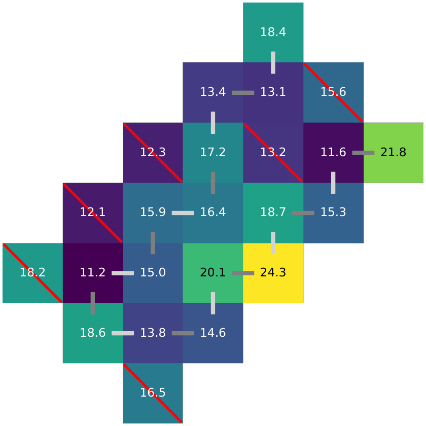
To improve the performance of the algorithm for a given number of qubits, we designed a graph traversal algorithm to select qubits based on diagnostic data taken during device calibration. Less weight was applied to and due to the availability of readout error mitigation techniques. We constructed a qubit graph where edges represent entangling gate connectivity and nodes represent qubits according to the Sycamore 23-qubit grid layout. The optimization was done by traversing all simple paths of fixed length (implemented according to Sedgewick 2001; Hagberg et al. 2008), and then scoring each path according to some function of the metrics for the subset of nodes and edges visited. Stated as an optimization problem, given an objective function scoring subsets of vertices and edges composing an Eulerian graph, this algorithm finds the maximum evaluation of over all possible graphs :
| (31) |
subject to the constraints , . Before applying , the heterogeneous calibration data were normalized to the range and inverted if they represented an error (as opposed to a fidelity). Letting the value of the -th category of calibration data for the i-th qubit be , and similarly the -th category of calibration for the i-th edge be , and defining as a scoring function applied to the -th processed calibration metric, our implementation of takes on the form
| (32) |
where and represent the calibration metrics corresponding to single and pairs of qubits respectively. We implemented as a logarithmic function for , , and metrics and a linear function for and metrics. Figure 7 shows the results of an example optimization overlaid on calibration results.
D.3 Readout error correction
Readout error resulting from relaxation and thermal excitation can be modelled by a stochastic bitflip process applied to the observed bitstrings. Here we describe an efficient and accurate technique for correcting readout error for quantum kernel methods.
Let describe the conditional probability for observing bitstring after exposing the bitstring to distinct bitflip channels, and let for describe the corresponding probability for observing bit “” after exposing the -th bit “” to a single bitflip channel. Then for the -th qubit, the metrics introduced in Appendix D.1 as and may be used to partially undo readout error by means of postprocessing. We define a response matrix elementwise as that contains as its elements the total probability for transition from bitstring to bitstring computed as the product of and corresponding to each individual bit:
| (33) |
For simplicity, we assume that each individual bitflip may be modelled as an independent process, although the techniques discussed here are readily applicable to a system of dependent bitflips if the bitflip likelihoods are experimentally measured in parallel. Then evidently,
| (34) |
Note that is generally asymmetric since typically . While multiplying by the set of observed bitstring frequencies would recover the prior distribution of bitstring frequencies with good fidelity, standard matrix inversion is subject to instabilities and is not tractable for even modest numbers of qubits.
Since only the frequency of the all-zero’s bitstring is necessary to compute , we implemented correction using a small subset of bitstring transition probabilities to perform quick and relatively high-fidelity readout error correction in post-processing. We generated and then truncated the full -dimensional basis to the bitstring space containing strings with Hamming weight for some -dependent resulting in a truncated response matrix . We then computed the pseudo-inverse and performed error correction by simple matrix multiplication on the array of experimental readout frequencies (similarly truncated). This simplification comes at the expense of knowledge about any other post-correction frequencies since the other bitstrings in the truncated space are off-center within the Hamming sphere of kept bitstrings, resulting in a bias in the inverted linear map.
We now analyze the effect of truncation on the readout error correction. The number of simultaneous readout error events (either relaxation or excitation) may be modelled as an induced random variable for . This distribution has expected value and an exponentially suppressed likelihood for simultaneous readout errors via the Chernoff bound . Thus a natural measure for the effect of Hamming weight truncation is the empirical probability allocated to the complement of the truncated subspace:
| (35) |
While Equation 35 describes the probability of events outside the truncated subspace, it does not directly translate to failure probability for truncated readout correction. To explore this effect numerically, we computed the output probability distributions for a 10-qubit quantum kernel circuit sampled for repetitions, and then introduced artificial readout error (using bitflip probabilities taken from the Sycamore processor) followed by roughly 5% Gaussian noise on the sampled distribution. Figure 8 shows the error distribution as well as the effect of correcting using an inverted truncated response matrix for a variety of kernel magnitudes and truncation weights. We observed similar behavior for 14 and 17-qubit simulated experiments; readout error for quantum kernel experiments may be corrected reasonably well using a small fraction of the full bitflip response matrix.
Figure 8 suggests a linear relationship between the kernel computed in the presence of readout error and the noiseless kernel . While readout error does not constitute a linear process in general (the underlying bitflip probabilities and bitstring distributions may be modified to give rise to arbitrary effects on within the bounds of Equation 41), by the arguments in Section B demonstrating such an effect in general would imply minimal effect of readout error on the corresponding classifier. The degree to which readout error plays a role in quantum kernel methods is therefore an important research area for implementation on near-term processors.
D.4 Crosstalk optimization
Cross-talk between two-qubit gates on implemented on superconducting processors can contribute to decoherence and decrease circuit fidelity. Since our choice of circuit ansatz requires entire layers of entangling gates, we conducted diagnostic runs to determine whether executing these gates sequentially (in different staggering patterns) could improve performance compared to executing the gates simultaneously. We found that the completely parallel execution of entangling gates achieved the lowest cross entropy with respect to noiseless simulation compared to partially sequential arrangements. Therefore all entangling gates in this experiment were run in parallel.
Appendix E Hardware error and performance
Figure 9 shows a typical outcome for sampled kernel elements compared to their true values as determined from noiseless simulation. Notably, all of the hardware outcomes are strongly biased towards zero as a result of decoherence. The observation that the SVM decision function is scale-invariant (Appendix B) suggests that the performance of an SVM trained using data subject to hardware error will only be affected to the degree that the sampled kernel elements differ from some linear transformation of the corresponding exact elements , so that the circuit fidelity and other typical metrics for hardware performance are not predictive of classifier performance in any obvious way. For instance, we achieved comparable test accuracy to noiseless simulation for qubits despite circuit fidelity in the neighborhood of .

E.1 Effects of readout error in quantum kernel methods
Since is estimated by computing the empirical probability of the all zeros bitstring , the effects of readout error may be bounded in a straightforward manner. The following analysis will consider readout error as the sole source of noise and ignore statistical effects and other sources of decoherence. The resulting bounds apply to only to the infinite-shot limit but will be shown to be approximately correct in the low-shot limit. As in Section D.3, we let describe the conditional probability for observing bitstring after exposing the bitstring to distinct bitflip channels, and let for describe the corresponding probability for observing ”” after exposing the -th bit ”” to a single bitflip channel. After exposing the all-zeros bitstring to a stochastic bitflip process repeatedly, the lowest possible value for occurs when no bitstrings transform into the all-zeros bitstring. The expected fraction of events remaining is
| (36) |
The maximum increase in the observed will result from transitions from other bitstrings into the all-zeros bistring. Intuitively this will occur almost entirely due to low-weight bitstrings with just a few bitflips. The probability of transition into the all-zeros bitstring from an arbitrary starting bitstring is , while the log-odds of each term in this product may be rewritten as
| (37) |
The total log-odds for transition into is then
| (38) |
which is in the form with , indicating a linear dependence of on . Since the logarithm is strictly increasing, the corresponding integer programming problem for maximizing is:
| (39) | ||||
| (40) |
where the second constraint avoids the trivial solution of the all-zeros bitstring. By inspection of Equation 38, implies that is strictly negative with the realistic assumption that . In this case, the solution maximizing Equation 39 must be a bitstring with weight 1 with a “1” at the position . Combined with Equation 36 this results in the bound:
| (41) |
Where describes the estimated kernel element after readout error has occurred. This bound is plotted in Figure 8 for one instance of a 10-qubit readout error calibration. The form of these bounds further justify the need for large kernels, since the bound becomes increasingly loose as approaches the magnitude of typical readout error probabilities on the quantum processor.
We now discuss the implementation of the readout error correction technique described in Appendix D.3. While routine calibration of the device returns diagnostic information on readout error probabilities and , these quantities may drift in the time between calibration and experiment resulting in lower quality readout correction. To account for drift, we periodically estimated and by preparing a sequence of random bitstrings and the complement and then measured in the computational basis. We then computed empirical bitflip likelihoods for measurements in parallel over the specific qubits used in each experiment and computed the time-averaged likelihoods to use for readout correction. We averaged over the different prepared states to reduce the impact of imperfect state preparation on measured outcomes.
Figure 10 shows learning curves computed for the 14-qubit experiment with and without readout correction for post-processing. While classifiers trained using error-corrected results are capable of achieving higher accuracies on the reserved test set, the choice of hyperparameter for improved test accuracy did not generally correspond to improved accuracies for the validation sets. Therefore, we could not consistently improve the classifier performance by applying readout correction and opted to present the results achieved without readout correction in Figure 4 in the main body.
E.2 Effects of statistical error on SVM accuracy
While recent work Liu et al. 2020 has established performance bounds relating SVM accuracy to statistical sampling error for quantum kernel methods, we conducted experiments using orders of magnitude fewer repetitions than necessary to achieve robust classification. In addition, modified SVM algorithms exist for processing noisy inputs in the data space Bi and Zhang 2005 but these modifications do not generalize to processing noise in the feature space (i.e. ). Given these limitations, we chose to explore the effects of statistical noise numerically to determine the relative impact of statistical noise on final classifier accuracy compared to other sources of error.
Figure 11 shows simulated trials of the type 2 circuits used for experimental runs. Each circuit was initially simulated with an full wavefunction simulator, and then the amplitude was used to sample repetitions from the implied binomial distribution . The sampled kernel elements were used to train and validate SVM classifiers following the procedure outlined in Section III.2. The results indicate there are diminishing returns in classifier accuracy beyond the repetitions we used for the experiments, but that this choice incurs classifier error compared to the infinite-shot limit. As expected, greater statistical noise results in less overfitting for the model.
E.3 Classifier results
Figure 12 shows the result of tuning the hyperparameter controlling the penalty for violating the SVM margin. The values resulting in optimal validation scores were then used to determine the final train/test scores reported in Figure 4 of the main body.