Fixed Viewpoint Mirror Surface Reconstruction under an Uncalibrated Camera
Abstract
This paper addresses the problem of mirror surface reconstruction, and proposes a solution based on observing the reflections of a moving reference plane on the mirror surface. Unlike previous approaches which require tedious calibration, our method can recover the camera intrinsics, the poses of the reference plane, as well as the mirror surface from the observed reflections of the reference plane under at least three unknown distinct poses. We first show that the 3D poses of the reference plane can be estimated from the reflection correspondences established between the images and the reference plane. We then form a bunch of 3D lines from the reflection correspondences, and derive an analytical solution to recover the line projection matrix. We transform the line projection matrix to its equivalent camera projection matrix, and propose a cross-ratio based formulation to optimize the camera projection matrix by minimizing reprojection errors. The mirror surface is then reconstructed based on the optimized cross-ratio constraint. Experimental results on both synthetic and real data are presented, which demonstrate the feasibility and accuracy of our method.
Index Terms:
Mirror surface, reconstruction, reflection, light path.I Introduction
3D reconstruction of diffuse surfaces has enjoyed tremendous success. These surfaces reflect light from a single incident ray to many rays in all directions, resulting in a constant appearance regardless of the observer’s viewpoint. Methods for diffuse surface reconstruction can therefore rely on the appearance of the object.
This paper considers mirror surfaces, which exhibit specular reflections and whose appearances are a reflection of the surrounding environment. Under (perfect) specular reflection, an incoming ray is reflected to a single outgoing ray. This special characteristic makes the appearance of a mirror surface viewpoint dependent, and renders diffuse surface reconstruction methods useless. Meanwhile, there exist many objects with a mirror surface in the man-made environment. The study of mirror surface reconstruction is therefore an important problem in computer vision.

|

|
| (a) | (b) |
In this paper, we assume the mirror surface reflects a light ray only once, and tackle the mirror surface reconstruction problem by adopting a common approach of introducing motion to the environment. Unlike previous methods which require a fully calibrated camera and known motion, we propose a novel solution based on observing the reflections of a reference plane undergoing an unknown motion with a stationary uncalibrated camera (see Fig. 1(a)). Note that the checkerboard pattern in Fig. 1(a) is used here only to demonstrate the overall reflection effects of the mirror surface. In our experiment, we display vertical and horizontal sweeping lines (e.g., the bottom row in Fig. 18) to establish reflection correspondences between images and the reference plane.
We first show that the relative poses of the reference plane can be estimated from the reflection correspondences established between the images and the reference plane under three unknown distinct poses. This enables us to construct a 3D ray piercing the reference plane at specific positions under different poses for each image point on the mirror surface. Given the set of 3D rays and their corresponding image points, we derive an analytical solution to recover the camera projection matrix through estimating the line projection matrix, which can be easily transformed back into a corresponding camera projection matrix. To make our solution more robust to noise, we use this closed-form solution as an initialization and optimize the camera projection matrix by minimizing reprojection errors computed based on a cross-ratio formulation for the mirror surface (see Fig. 1(b)). The mirror surface is then reconstructed based on the optimized cross-ratio constraint. The key contributions of this work are
- 1.
To the best of our knowledge, the first mirror surface reconstruction solution under an unknown motion of a reference plane and an uncalibrated camera.
- 2.
A closed-form solution for recovering the relative 3D poses of the reference plane from reflection correspondences.
- 3.
A closed-form solution for estimating the camera projection matrix from reflection correspondences.
- 4.
A cross-ratio based nonlinear formulation that allows a robust estimation of the camera projection matrix together with the mirror surface.
We have presented preliminary results of this work in [1]. This paper extends [1] as follows: 1) We include more experimental results. In particular, we reconstructed a mirror hood and the results, in terms of quality, are similar to those of the previous experiments. This further validates the effectiveness of our approach. 2) We include details of the reference plane pose estimation from reflection correspondences and the related experimental results to make our work more self-contained. 3) We quantify the surface of an object that can be reconstructed using our method by deriving a relation among the surface normal, the distance between the reference plane and the surface, and the size of the reference plane. 4) We include discussions on the degeneracy as well as the limitations of our methods. 5) We describe the conversion between the point projection matrix and the line projection matrix in detail.
The rest of the paper is organized as follows. Section II briefly reviews existing techniques in the literature for shape recovery of mirror surfaces. Section III describes our data acquisition setup and our closed-form solution for 3D poses estimation of the reference plane. Section IV introduces our closed-form solution for camera projection matrix estimation. Section V describes our cross-ratio based nonlinear formulation. Section VI quantifies the surface that can be reconstructed by our method and discusses the degeneracy. Experimental results are presented in Section VII, followed by conclusions in Section VIII.
II Related Work
Great efforts have been devoted to the problem of mirror surface recovery [2, 3, 4]. Based on the assumed prior knowledge, shape recovery methods for mirror surfaces can be classified into those assuming an unknown distant environment and those assuming a known nearby environment.
Under an unknown distant environment, a set of methods referred to as shape from specular flow (SFSF) have been proposed. In [5], Oren and Nayar successfully recovered a 3D curve on the object surface by tracking the trajectory of the reflection of a light source on the mirror surface. However, it is difficult to track a complete trajectory since the reflected feature will be greatly distorted near the occluding boundary of an object. Roth and Black [6] introduced the concept of specular flow and derived its relation with the 3D shape of a mirror surface. Although they only recovered a surface with a parametric representation (e.g., sphere), their work provided a theoretical basis for the later methods. In [7, 8], Adato et al. showed that under far-field illumination and large object-environment distance, the observed specular flow can be related to surface shape through a pair of coupled nonlinear partial differential equations (PDEs). Vasilyev et al. [9] further suggested that it is possible to reconstruct a smooth surface from one specular flow by inducing integrability constraints on the surface normal field. In [10], Canas et al. reparameterized the nonlinear PDEs as linear equations and derived a more manageable solution. Although SFSF achieves a theoretical breakthrough in shape recovery of mirror surfaces, the issues in tracking dense specular flow and solving PDEs still hinder their practical use. In [11], Sankaranarayanan et al. developed an approach that uses sparse specular reflection correspondences instead of specular flow to recover a mirror surface linearly. Their proposed method is more practical than the traditional SFSF methods. Nevertheless, their method requires quite a number of specular reflection correspondences across different views, which are difficult to obtain due to the distorted reflections on the mirror surface.
Under a known nearby environment, a different set of methods for shape recovery of mirror surfaces can be derived. The majority of these methods are based on the smoothness assumption on the mirror surface. Under this assumption, one popular way is to formulate the surface recovery into the problem of solving PDEs. In [12, 13], Savarese and Perona demonstrated that local surface geometry of a mirror surface can be determined by analyzing the local differential properties of the reflections of two calibrated lines. Following the same fashion, Rozenfeld et al. [14] explored the 1D homography relation between the calibrated lines and the reflections using sparse correspondences. Depth and first order local shape are estimated by minimizing a statistically correct measure, and a dense 3D surface is then constructed by performing a constrained interpolation. In [15], Liu et al. proved that a smooth mirror surface can be determined up to a two-fold ambiguity from just one reflection view of a calibrated reference plane. Another way to formulate the mirror surface recovery is by employing normal consistency property to refine visual hull and/or integrate normal field. In [16], Bonfort and Sturm introduced a voxel carving method to reconstruct a mirror surface using a normal consistency criterion derived from the reflections of some calibrated reference planes. In order to get a better view for shape recovery, they further proposed that the camera does not need to face the reference plane, and the shape can be well recovered by using a mirror to calibrate the poses of the reference plane [17, 18]. In [19], Nehab et al. formulated the shape recovery as an image matching problem by minimizing a cost function based on normal consistency. In [20], Weinmann et al. employed a turntable setup with multiple cameras and displays, which enables the calculation of the normal field for each reflection view. The 3D surface is then estimated by a robust multi-view normal field integration technique. In [21], Balzer et al. deployed a room-sized cube consisting of six walls that encode/decode specular correspondences based on a phase shift method. The surface is then recovered by integration of normal fields. Tin et al. [22] introduced a two-layer LCD setup, which contains a pair of perpendicular linear polarizers for establishing correspondences between the illumination rays and camera rays. After calibrating the camera and LCDs, the surface can be reconstructed by solving a joint optimization problem. In [23], Lu et al. introduced a setup to generate a polarization field using a commercial LCD with the top polarizer removed and modeled the liquid crystals as polarization rotators. Another approach is to reconstruct the individual light paths based on the law of reflection. Kutulakos and Steger [24] showed that a point on a mirror surface can be recovered if the positions of two reference points are known in space and reflected to the same image point in a single view, or the positions of two reference points are known and are reflected by the same surface point to two different views.
Note that calibration plays an important role in all the above methods that assume a known nearby environment. Commonly, a reference plane with a known pattern is used as the known environment. In order to produce a good view of its reflections on the specular surface, the reference plane is often placed side-by-side with the camera. This results in the camera not being able to see the reference plane directly, making the calibration of the setup non-trivial. Traditional methods calibrate the poses of the reference plane by introducing an extra reference plane in the field of view of the camera, and an extra camera looking at both reference planes. In [18], Sturm and Bonfort used a planar mirror to allow the camera to see the reference plane through reflection. The pose of the reference plane can be obtained by placing the auxiliary mirror in at least three different positions. Generally, multiple reference plane positions are needed for recovering a large area of the mirror surface. However, the literature becomes comparatively sparse when it comes to automatic pose estimation of the reference plane in mirror surface recovery. Liu et al. [25] proposed an automatic motion estimation method by constraining the motion of the reference plane to a pure translation. Although they can achieve a simple closed-form solution for the motion estimation problem, their method cannot handle general motion. Besides, their method requires calibrating the intrinsics of the camera as well as the initial pose of the reference plane. In fact, most, if not all, of the methods that assume a known nearby environment require the camera(s) to be fully calibrated. In contrast, we neither require the calibration of the reference plane poses, nor require the calibration of the camera, and make no assumption on the smoothness of the mirror surface. Our proposed approach can automatically calibrate the setup as well as reconstruct the mirror surface using the observed reflections of the reference plane.
A cross-ratio constraint has been used to estimate mirror position and camera pose for axial non-central catadioptric systems [26, 27], and produce more point correspondences in the context of 3D reconstruction [28]. In this work, we incorporate cross-ratio constraint in our formulation to simultaneously optimize the camera projection matrix and recover the mirror surface.
III Acquisition Setup and Plane Pose Estimation
III-A Acquisition Setup
Figure 2 shows the setup used for mirror surface reconstruction. Consider a pinhole camera centered at observing the reflections of a moving reference plane on a mirror surface . Let be a point on the plane at its initial pose, denoted by , which is reflected by a point on to a point on the image plane . Suppose the reference plane undergoes an unknown rigid body motion, and let and denote the plane at its two new poses. Let and be points on and , respectively, which are both reflected by on to the same image point on . , and are referred to as reflection correspondences of the image point . Since reflection correspondences must lie on the same incident ray, it follows that they must be colinear in 3D space. This property will be used to derive a constraint for computing the poses of the moving reference plane relative to its initial pose (see Section III-B).
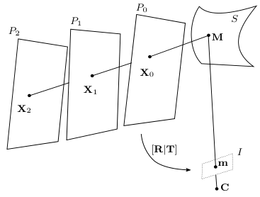
III-B Plane Pose Estimation
Referring to the setup shown in Fig. 2. Let the rigid body motion between and be denoted by (), where and are the rotation (matrix) and translation (vector) respectively. Similarly, let () denote the rigid body motion between and . Let , , and be points on , and , respectively, that lie on the same incident light path. The 2D coordinates of on the plane are = , where . Their 3D coordinates, , , w.r.t can be written as
where , , , and denotes the th column of . The unknown motion parameters are now embedded in and . Since and are colinear, it follows that
| (1) |
where and denote the th row of and respectively. The following two constraints can be derived from Equation (1):
| (2) |
where and .
Given points , where , , and , we can formulate the problem as solving a linear system
| (3) |
where
| (4) |
and denote the th row of and respectively, and denotes Kronecker tensor product. contains unknowns in total. Since each incident ray provides two constraints, we need at least 12 incident rays (i.e., reflection correspondences) to solve all the unknowns.
Note that the st and th columns of are identical, the nullity of E must be two in order to have a non-trivial solution. Therefore, we first apply SVD to get a solution space spanned by two solution basis vectors, and . We then parameterize as
| (5) |
where and are two scale parameters. Now there are unknowns in total. By enforcing the element-wise equality of Equation (4) and Equation (5), we have bilinear and linear equations to solve , , and . Furthermore, we have and since . Thus,
Similarly, we can show . Obviously, not all of the obtained constraints are independent, and new constraints should be applied in order to solve all the unknowns. Since the first two columns of and come from the first two columns of and respectively, the orthonomality property will provide extra constraints, which leads to a closed-form solution for the unknown motion parameters and the two scale parameters. We use the Symbolic Math Toolbox in Matlab to solve them (refer to the supplementary for more details).
IV Projection Matrix Estimation
In this section, we first briefly review the line projection matrix. We then derive a linear method for obtaining a closed-form solution to the line projection matrix of a camera from the reflection correspondences.
IV-A Line Projection Matrix
Using homogeneous coordinates, a linear mapping can be defined for mapping a point in 3D space to a point in a 2D image, i.e.,
| (6) |
where is a matrix known as the camera (point) projection matrix. Similarly, using Plücker coordinates11 1 A brief review of Plücker coordinates is given in the supplementary., a linear mapping can be defined for mapping a line in 3D space to a line (in homogeneous coordinates) in a 2D image, i.e.,
| (7) |
where is a matrix known as the line projection matrix and is the dual Plücker vector22 2 Given a Plücker vector , its dual Plücker vector is . of . Note that each row () of represents a plane (in homogeneous coordinates) that intersects at the optical center. Dually, each row () of represents a line that intersects at the optical center (see Fig. 3). It follows that a valid line projection matrix must satisfy
| (8) |
where .

|

|
| (a) | (b) |
A line projection matrix can be converted to its corresponding camera (point) projection matrix, and vice versa. Details of the conversion are given in the supplementary.
IV-B Estimating the Line Projection Matrix
To estimate the line projection matrix of the camera, we first apply our method described in Section III-B to recover the relative poses of the reference plane under three distinct poses using reflection correspondences established between the images and the reference plane. We can then form a 3D Plücker line from the reflection correspondences of each observed point in the image. Note that, by construction, must lie on the projection of , i.e.,
| (9) |
Given a set of 3D space lines constructed for a set of image points , the constraint derived in (9) can be arranged into
| (10) |
where and
| (11) |
The line projection matrix of the camera can then be estimated by solving
| (12) |
subject to . The line projection matrix thus obtained can be transformed into a point projection matrix and vice versa. Note that, however, (12) minimizes only algebraic errors and does not enforce (8). The solution to (12) is therefore subject to numerical instability and not robust in the presence of noise. Instead of solving (12), we can minimize the geometric distance from each image point to the projection of the corresponding 3D line. Let be the projection of the 3D line corresponding to an image point . can be estimated by solving
| (13) |
subject to , where is the Frobenius norm of . A straight-forward approach to enforce (8) is by incorporating it as a hard constraint in (13). However, experiments using a number of state-of-the-art optimization schemes show that such a solution often converges to local minima.
IV-C Enforcing Constraints
Given a proper camera projection matrix, the corresponding line projection matrix will automatically satisfy (8). However, given an improper line projection matrix not satisfying (8), the corresponding camera projection matrix cannot be decomposed into one with proper intrinsic and extrinsic parameters. Based on this observation, we propose to enforce (8) through ensuring a proper decomposition of the camera projection matrix.
Consider a simplified scenario where the principal point (which is often located at the image centre) is known. After translating the image origin to the principal point, the camera projection matrix can be expressed as
and the corresponding line projection matrix (refer to the supplementary for the conversion) can be expressed as
| (14) |
where
| (15) |
with and . (10) can then be rewritten as
| (16) |
where , and is a diagonal matrix with for , for , and for .
With known and , can be estimated by solving (16). Since only depends on the elements of and , it can be converted to a point projection matrix (refer to the supplementary for the conversion) in the form of . The magnitude of is determined by the orthogonality of , and its sign is determined by the sign of . Hence, given the camera intrinsics, the camera extrinsics can be recovered using the reflection correspondences.
In Section V, we tackle the problem of unknown camera intrinsics by formulating the problem into a nonlinear optimization by minimizing reprojection errors computed based on a cross-ratio formulation for the mirror surface. For initialization purpose, we assume being located at the image center, and . We choose a rough range of and for each sample value of within the range, we estimate and by solving (16). The point to line distance criterion in (13) is applied to find the best focal length . A camera projection matrix can then be constructed using , , and that satisfies all the above mentioned constraints.
V Cross-ratio Based Formulation
In this section, we obtain the camera projection matrix and the mirror surface by minimizing reprojection errors. We will derive a cross-ratio based formulation for recovering a 3D point on the mirror surface from its reflection correspondences. Note that minimizing point-to-point reprojection errors can provide a stronger geometrical constraint than minimizing the point-to-line distances in (13) (see Fig. 4).


Consider a point on the mirror surface (see Fig. 5). Let , and be its reflection correspondences on the reference plane under three distinct poses, denoted by , and , respectively. Suppose , , and are projected to the image as , , and respectively. We observe that the cross-ratios and must be identical, i.e.,
| (17) |
where denotes the directed ray (vector) from to and is the length of the vector. Let be the distance between and (i.e., ), from (17)
| (18) |
Given the projection matrix, , , and , the surface point can be recovered as
| (19) |
We optimize the projection matrix by minimizing the reprojection errors, i.e.,
| (20) |
where is the observation of , , and 33 3 We used angle-axis representation for rotation, i.e., , where is the rotation angle and is the unit rotation axis.. To obtain in (18), we also project the three reflection correspondences of to the image using . We initialize using the method proposed in Section IV, and solve the optimization problem using the Levenberg-Marquardt method. Given the estimated projection matrix, the mirror surface can be robustly reconstructed by solving (17)-(19).
VI Discussion
VI-A Object Analysis
We analyze the surface points that can be reconstructed by our proposed method using an example as shown in Fig. 6, where a fixed camera centered at is viewing a mirror surface , and a reference plane is placed beside the surface. Consider the visual ray of a pixel for the surface point . The angle between the incident ray and the reflected ray (visual ray) will restrict the surface point that can be reconstructed by our method. Given a reference plane as in Fig. 6, the minimum angle between the incident ray and the reflected ray is leading to a surface normal , while the maximum angle is leading to a surface normal . The surface point can be reconstructed by our method when its normal lies in the range between and . This range can be represented as the angle , which is related to the distance between the surface and the reference plane, the size of the reference plane, and the relative pose between the camera and the reference plane.
Let , , , and . According to the law of reflection, we have
| (21) | |||
| (22) |
It follows that
| (23) | ||||
From (23), we can see that a larger size of the reference plane and/or a closer distance between the surface and the reference plane will result in a larger surface region that can be reconstructed by our method. Note that however according to (21), it is not necessary for to be infinite large as we have to ensure (i.e., ) otherwise the camera will not perceive the reflected ray .
Thus, we can conclude that if the surface normals are distributed within the range defined by , the whole surface can be reconstructed by our method. For a surface with a broader normal distribution, we can recover it by increasing the range via using a large enough reference plane and placing the reference plane at a location not too far away from the surface. In addition, placing the reference plane at multiple locations facing different (visible) regions of the object can also help enlarge the region that can be reconstructed. Alternatively, a cubic room like the one built in [21] can be used to enlarge the normal range that can be reconstructed by our method. However, our method requires moving each side of the room to three different locations, which makes it difficult to build such a room.
In addition, we discuss the relationship among the object size, distance from the camera to the object, and distance from the reference plane to the object as shown in Fig. 7. A camera centered at observes the mirror surface . and are the normals at surface points and . For simplicity, let . We then construct points and with and . A virtual camera center at can be formed by extending and . Let , , , and , we have . The maximum size of the surface that can be reconstructed by our method is then approximated by . Note that we use a planar surface here only for discussion, while planar surfaces correspond to the degenerate case of our method as will be discussed next. As long as there are some normal variations between and on , the above discussion is still a valid approximation.
Lastly, it is worth noting that we assume the surface is perfectly reflective and our formulation depends on the law of reflection. Therefore, our method may not work for other mirror-like surfaces that do not follow the law of reflection. Meanwhile, for some mirror objects, the energy of the incident rays are not fully reflected due to the surface material. For such cases, the brightness of the sweeping stripes for correspondence estimation will be low, bringing more difficulties in identifying the peak from the intensity profile (see Fig. 8), thus reducing the accuracy of camera projection matrix estimation and shape reconstruction.
VI-B Degeneracy
In order to obtain 3D line correspondences, we proposed the method in Section III-B to estimate relative poses of the reference plane. However, there do exist degenerate cases. In particular, the relative poses of the reference plane cannot be uniquely determined in the following cases: (1) The specular object is of a planar, elliptical, parabolic or hyperbolic mirror; and (2) the arrangement of such mirror surfaces and the pinhole camera forms a central catadioptric system; namely the pinhole camera and the mirror surfaces form a single effective viewpoint. If the unknown mirror surface and the camera form a central catadioptric system with a single effective viewpoint, the relative pose estimation between reference planes (e.g., , , ) is equivalent to the camera calibration process described in [29]. As demonstrated in [29], the poses cannot be determined if the reference plane undergoes pure translation without knowing the translation direction. If the reference plane is placed at three general positions, the poses are estimated up to one scale ambiguity. As analysed in [30], a pinhole camera viewing a sphere does not form a central catadioptric system in general if the distance between the pinhole and effective viewpoint is larger than the radius. If the camera is located at the centre of the sphere, it indeed forms a central catadioptric system, which however differs from our experimental setup.
In addition, when in Fig. 5 are close to each other, while are further away to each other, our cross-ratio based formulation will be more sensitive to noise and a small error in the pixel domain will result in a large error in 3D points estimation. Actually, this is on par with small baseline triangulation as described in [31], which is generally more sensitive to noise.
VII Evaluation
To demonstrate the effectiveness of our method, we evaluate it using both synthetic and real data. We first evaluate the effectiveness of our proposed approach for estimating the relative poses of the reference plane (Section III-B). We then show that our approach can faithfully reconstruct the mirror surfaces. The source code of our method can be found at https://github.com/k-han/mirror.
VII-A Relative Pose Estimation of the Reference Plane
To evaluate the performance of our reference plane pose estimation presented in Section III-B, we generated synthetic data using two spheres. The spheres have a radius of 300 . The reference plane used has a dimension of 20002000 and was placed at three different poses denoted by , , and respectively. The reflection correspondences were obtained via ray tracing. To evaluate the robustness of our method, we added Gaussian noise to the reflection correspondences on the reference plane with standard deviations ranging from 0 to 3.0 . The errors were reported as the average value over 50 trials of the experiments for each noise level (Gaussian noise standard deviation). Specifically, we reported the errors in the relative rotation matrix in terms of the angle of the rotation induced by , where denotes the ground truth rotation matrix. We reported the errors in the translation vector in terms of the angle () between and , where denotes the ground truth translation vector and . In Fig. 9, we show the estimation errors for (, ) and (, ). It can be seen that the errors increase with the noise level, while the magnitude of the errors are quite small, demonstrating that our relative pose estimation method is robust to the noise.
| (a) | (b) | (c) |
VII-B Recovery of Projection Matrix and Mirror Surface
VII-B1 Synthetic Data Experiments
We employed a reflective Stanford bunny and a reflective engine hood created by [21] to generate our synthetic data. The bunny has a dimension of and surface points, while the hood has a dimension of and surface points. The images have a resolution of pixels. Figure 10(a) shows the reflective appearances of the bunny and the hood. In their original data, the bunny (hood) was placed in a cubic room, with each side of the room working as a reference plane. The reference plane has a dimension of . The center of the room was defined as the world origin. A camera was placed in the room viewing the bunny (hood). Since our method requires reflection correspondences under three distinct poses of the reference plane, we introduced two additional planes for each side of the room and obtained the reflection correspondences through ray tracing.

|
||

|
||
| (a) | (b) | (c) |

|

|

|

|

|

|
|

|

|

|

|

|

|

| |

|
|

|

|

|

|
|

|

|

|

|

|

|

| |
| ground truth | no noise | noise lv: | noise lv: | noise lv: |
| bunny | ||||||||
|---|---|---|---|---|---|---|---|---|
| hood | ||||||||
- •
The ground truth for the intrinsic parameters are , , and . The norm of translation vectors are and for and , respectively.
To evaluate the performance of our method, we added Gaussian noise to the 2D reflection correspondences on the reference plane with standard deviations ranging from to . The reflection correspondences are the input of our method and essential to the performance. It is difficult to obtain high quality reflection correspondences due to the distortion caused by the reflection of the mirror surface. Thus we added the noise to the reflection correspondences. The typical intensity profile for the x- or y-coordinate is a bell-shaped curve (see Fig. 8 for an example), which has a similar characteristic as Gaussian distribution, hence we choose Gaussian noise to model the possible noises in the 2D correspondences. We initialized the projection matrix using the method described in Section IV. The optimized projection matrix together with the 3D surface points were obtained by minimizing reprojection errors computed based on our cross-ratio formulation. In Table I, we compared: 1) linear solution by solving (12) in Section IV-B, denoted as ; 2) linear solution by solving (16) after enforcing the constraints in Section IV-C, denoted as ; and 3) cross-ratio based non-linear solution by solving (20) in Section V, denoted as . It can be seen that our cross-ratio based formulation can effectively improve the linear solutions. Figure 10(b) and (c) depict the root mean square (RMS) reprojection errors and reconstruction errors, respectively, under different noise levels. It can be seen that the reprojection errors and the reconstruction errors increase linearly with the noise level. The magnitude of the reconstruction errors is relatively small compared to the size of the object. Figure 11 shows the reconstructed point clouds and surfaces. Table II shows a quantitative comparison of our estimated projection matrices w.r.t the ground truth. Among all noise levels, the errors are below for , , , and , and angular errors are below for and .
Moreover, as the quantization noise, which obeys the uniform distribution, is also typical in real situations, we further verify the robustness of our approach to the quantization noise by adding the uniform noise in the range of to the 2D pixel locations. The results are reported in Table III and Fig. 12. The errors increase linearly with the noise level while the estimation errors are small, revealing that our approach is robust to quantization noise.
Besides, we compared our method with state-of-the-art mirror surface reconstruction method in [15] under smooth surface assumption and calibrated setup. Note that [15] assumes the mirror surface is continuous. In order to make a fair comparison, we performed the experiment on a sphere patch under the same setup with the Stanford bunny and engine hood datasets. Fig. 13 depicts the comparison between fully calibrated ([15]) and uncalibrated (proposed) methods. The overall reconstruction accuracies are similar. While our result is not as smooth as that of [15] due to our point-wise reconstruction. Their result shows a global reconstruction bias due to the B-spline parameterization for the surface (see Fig. 13).

|

|

|
| 2.22/2.21 | ||||||||
|---|---|---|---|---|---|---|---|---|
| 3.07/3.06 |
- •
denotes the mean pixel offsets introduced by the lens distortion.

|

|

|

|

|
| ground truth |
We consider the ideal pinhole camera model, therefore the potential lens distortion is not taken into account in our formulation. In practice, the lens may have radial and tangential distortion [33]. The one-parameter radial distortion is the most common form of distortion, which can be described by
| (24) |
where and are the undistorted and distorted pixel locations in normalized image coordinates (), is the radial distortion coefficient (positive/negative radial distortion is also known as barrel/pincushion distortion) of the lens and . To verify the robustness of our method to the lens distortion, we thoroughly evaluate the performance of our method on bunny and hood shapes by introducing radial distortion of different levels. After introducing distortion, the pixel locations are denormalized to the original magnitude for camera pose estimation and surface reconstruction. We vary the distortion coefficient and measure the reconstruction errors on bunny and hood (see Fig. 14). In Table IV, we show the results of our approach under with of /. It can be seen that our method is generally robust to the lens distortion.
We further compare the surface reconstruction results between the ray triangulation and our cross-ratio based method in Fig. 15, given the camera projection matrix estimated by our method. It can be seen that with the estimated camera projection matrix, the reconstruction accuracy of ray triangulation is on par with our cross-ratio based formulation. As the surface points can be obtained as the by-product of our cross-ratio based methods, the extra ray triangulation is no longer needed. Meanwhile, comparing with the ray triangulation results using our camera projection matrix initialization method in Section IV-C, our cross-ratio based method can significantly improve the reconstruction results. In addition, we also explored the triangulation counterpart for the optimization problem in (20), by simply replacing the 3D point formulation in (19) with ray triangulation (i.e., triangulating the incident and the reflected (visual) rays). The results are reported in Table V and Fig. 17. Though the triangulation based formulation can also improve the results obtained by our constrained linear solution introduced in Section IV-C (Table I vs Table V), the cross-ratio formulation performs notably better. Both formulations aim to minimize the point-to-point reprojection error. However, as our cross-ratio based formulation also enforces the cross-ratio constraint during optimization, it includes more geometric regularization than ray triangulation based formulation, leading to better performance.
After obtaining the camera projection matrix and surface points by our cross-ratio based method, we can obtain the normal by simply calculating the bisector of the visual ray and incident ray. Figure 16 shows the normal estimation results on hood. It can be seen that our method can estimate accurate normals. In this work, we focus more on recovering the point cloud because it contains the actual scale information of the object.
VII-B2 Real Data Experiments

- •
and denote the results of sauce boat and two spheres respectively. The subscripts , , and stand for experiments under (1) an uncalibrated camera and calibrated plane poses, (2) a calibrated camera and uncalibrated plane poses, and (3) an uncalibrated camera and uncalibrated plane poses, respectively. The ground truth for the intrinsic parameters are , , and . stands for the RMS reconstruction error.

|

|

|

|

|

|

|

|
| (a) | (b) | (c) | (d) |

|

|

|

|

|

|

|

|
| (e) | (f) | (g) | (h) |
We evaluated our method on a sauce boat and two spheres respectively (see Fig. 18). We captured images using a digital camera with a - lens. A LCD monitor was used as a reference plane and was placed at three different locations. We follow [24, 34, 35] to display sweeping stripes on the monitor to establish reflection correspondences. In particular, at each location, the LCD monitor shows a thin stripe sweeping across the screen in vertical direction and then in horizontal direction. For each position of the sweeping stripe, we capture an image. We then obtain a sequence of images w.r.t the vertically sweeping stripe and a sequence of images w.r.t the horizontally sweeping stripe. We can then obtain the correspondence on the reference plane for each image point by examining its corresponding two sequences of intensity values. The position of the stripe that produces the peak intensity value in each sweeping direction then gives the position of the correspondence on the reference plane. In order to improve the accuracy of the peak localization, we fit a quadratic curve to the intensity profile in the neighborhood of the sampled peak value, and solve for the exact peak analytically.
After establishing reflection correspondences, we first estimated the relative poses of the reference plane using our method described in Section III-B. We then formed 3D lines from the reflection correspondences on the reference plane under the two poses that were furthest apart (e.g., and in Fig. 5). These 3D lines were used to obtain a preliminary solution of projection matrix using the linear method in Section IV, which was then used to initialize the nonlinear optimization described in Section V.
To evaluate our method, we calibrated the camera and reference plane poses using the Camera Calibration Toolbox for Matlab [36]. We used the calibration result to estimate the surface and treated it as the ground truth. This result was compared against the result obtained using 1) uncalibrated camera and calibrated plane poses, 2) calibrated camera and uncalibrated plane poses, and 3) uncalibrated camera and uncalibrated plane poses. Fig. 19 shows the reconstructed surfaces and Table VI shows the numerical errors. We aligned each estimated surface with the ground truth by a rigid body transformation using the method in [37] before computing the reconstruction error. The RMS reconstruction errors are below . and errors are below . , and errors are below . The angular errors are below for and below for . The errors in intrinsics and extrinsics are larger than those in the synthetic experiments. This is reasonable since accurate reflection correspondences in real cases are difficult to obtain due to the large and complex distortion caused by the mirror surface and varying lighting condition. Besides, degradation from optics, such as optics aberrations, will also introduce errors for establishing reflections correspondences. The quality of the reflection correspondences is also a key factor for other existing mirror surface reconstruction methods. Note that existing methods are designed under certain assumptions (e.g., convex, continuity, etc), and their setups are carefully tailored or require special equipments. Besides, there is no publicly available dataset that can serve as a benchmark for existing methods. As a result, it is challenging to make a fair comparison with existing methods on real data. Therefore, we do not include comparison with other existing methods on real data.
VIII Conclusions
A novel method is introduced for mirror surface reconstruction. Our method works under an uncalibrated setup and can recover the camera intrinsics and extrinsics, along with the surface. We proposed an analytical solution for the reference plane relative pose estimation, a closed-form solution for camera projection matrix estimation, and a cross-ratio based formulation to achieve a robust estimation of both camera projection matrix and the mirror surface. The proposed method only needs reflection correspondences as input and removes the restrictive assumptions of known motions, continuity of the surface, and calibrated camera(s) that are being used by other existing methods. This greatly simplifies the challenging problem of mirror surface recovery. We believe our work can provide a meaningful insight towards solving this problem.
Our method does have a few limitations. We assume the surface is perfectly reflective and our formulation depends on the law of reflection. Thus our method may not work for other mirror-like surfaces that do not follow the law of reflection, or mirror surfaces that do not reflect the full energy of the incident rays. Although our cross-ratio based formulation does not encounter degenerate cases, degenerate cases may occur in the relative pose estimation of the reference plane. Efforts are needed to explore methods without degeneracy for estimating the relative poses of the reference plane from reflection correspondences. Meanwhile, the region that can be reconstructed by our method depends on the size of the reference plane. For mirror surfaces with complex normal distribution, the reference plane may need to be carefully placed at different locations facing different regions of the mirror surface, and the reference plane should be moved three times at each location. Despite an increased number of images, extra efforts are also required to fuse these reconstructed regions together. Besides, in our formulation, we did not consider inter-reflection, which is likely to happen for regions with relatively sharp changes in the mirror surface. In the future, we would like to develop methods to recover complete surfaces and further investigate inter-reflection cases.
Acknowledgement
This project is supported by a grant from the Research Grant Council of the Hong Kong (SAR), China, under the project HKU 17203119 and a grant (DE180100628) from Australian Research Council (ARC).
References
- [1] K. Han, K.-Y. K. Wong, D. Schnieders, and M. Liu, “Mirror surface reconstruction under an uncalibrated camera,” in CVPR, 2016, pp. 1772–1780.
- [2] J. Balzer and S. Werling, “Principles of shape from specular reflection,” Measurement, vol. 43, no. 10, pp. 1305–1317, 2010.
- [3] I. Ihrke, K. N. Kutulakos, H. P. A. Lensch, M. Magnor, and W. Heidrich, “Transparent and specular object reconstruction,” Computer Graphics Forum, vol. 29, pp. 2400–2426, 2010.
- [4] I. Reshetouski and I. Ihrke, “Mirrors in computer graphics, computer vision and time-of-flight imaging,” Lect. Notes Comput. Sc., vol. 8200, pp. 77–104, 2013.
- [5] M. Oren and S. K. Nayar, “A theory of specular surface geometry,” IJCV, vol. 24, no. 2, pp. 105–124, 1996.
- [6] S. Roth and M. J. Black, “Specular flow and the recovery of surface structure,” in CVPR, 2006, pp. 1869–1876.
- [7] Y. Adato, Y. Vasilyev, O. Ben-Shahar, and T. Zickler, “Toward a theory of shape from specular flow,” in ICCV, 2007, pp. 1–8.
- [8] Y. Adato, Y. Vasilyev, T. Zickler, and O. Ben-Shahar, “Shape from specular flow,” PAMI, vol. 32, no. 11, pp. 2054–2070, 2010.
- [9] Y. Vasilyev, T. Zickler, S. Gortler, and O. Ben-Shahar, “Shape from specular flow: Is one flow enough?” in CVPR, 2011, pp. 2561–2568.
- [10] G. D. Canas, Y. Vasilyev, Y. Adato, T. Zickler, S. Gortler, and O. Ben-Shahar, “A linear formulation of shape from specular flow,” in ICCV, 2009, pp. 191–198.
- [11] A. Sankaranarayanan, A. Veeraraghavan, O. Tuzel, and A. Agrawal, “Specular surface reconstruction from sparse reflection correspondences,” in CVPR, 2010, pp. 1245–1252.
- [12] S. Savarese and P. Perona, “Local analysis for 3d reconstruction of specular surfaces.” in CVPR, 2001, pp. 738–745.
- [13] S. Savarese and P. Perona, “Local analysis for 3d reconstruction of specular surfaces – part ii,” in ECCV, 2002, pp. 759–774.
- [14] S. Rozenfeld, I. Shimshoni, and M. Lindenbaum, “Dense mirroring surface recovery from 1d homographies and sparse correspondences,” PAMI, vol. 33, no. 2, pp. 325–337, 2011.
- [15] M. Liu, R. Hartley, and M. Salzmann, “Mirror surface reconstruction from a single image,” PAMI, vol. 37, no. 4, pp. 760–773, 2015.
- [16] T. Bonfort and P. Sturm, “Voxel carving for specular surfaces,” in ICCV, 2003, pp. 691–696.
- [17] T. Bonfort, P. Sturm, and P. Gargallo, “General specular surface triangulation,” in ACCV, 2006, pp. 872–881.
- [18] P. Sturm and T. Bonfort, “How to compute the pose of an object without a direct view,” in ACCV, 2006, pp. 21–31.
- [19] D. Nehab, T. Weyrich, and S. Rusinkiewicz, “Dense 3d reconstruction from specularity consistency,” in CVPR, 2008, pp. 1–8.
- [20] M. Weinmann, A. Osep, R. Ruiters, and R. Klein, “Multi-view normal field integration for 3d reconstruction of mirroring objects.” in ICCV, 2013, pp. 2504–2511.
- [21] J. Balzer, D. Acevedo-Feliz, S. Soatto, S. Höfer, M. Hadwiger, and J. Beyerer, “Cavlectometry: Towards holistic reconstruction of large mirror objects,” in International Conference on 3D Vision (3DV), 2014, pp. 448–455.
- [22] S.-K. Tin, J. Ye, M. Nezamabadi, and C. Chen, “3d reconstruction of mirror-type objects using efficient ray coding,” in ICCP, 2016.
- [23] J. Lu, Y. Ji, J. Yu, and J. Ye, “Mirror surface reconstruction using polarization field,” in ICCP, 2019, pp. 1–9.
- [24] K. N. Kutulakos and E. Steger, “A theory of refractive and specular 3D shape by light-path triangulation,” IJCV, vol. 76, pp. 13–29, 2008.
- [25] M. Liu, K.-Y. K. Wong, Z. Dai, and Z. Chen, “Specular surface recovery from reflections of a planar pattern undergoing an unknown pure translation,” in ACCV, vol. 2, 2010, pp. 647–658.
- [26] L. Perdigoto and H. Araujo, “Calibration of mirror position and extrinsic parameters in axial non-central catadioptric systems,” CVIU, vol. 117, pp. 909–921, 2013.
- [27] S. Ramalingam, P. Sturm, and S. K. Lodha, “Towards complete generic camera calibration,” in CVPR, 2005, pp. 1093–1098.
- [28] S. Ramalingam, M. Antunes, D. Snow, G. Hee Lee, and S. Pillai, “Line-sweep: Cross-ratio for wide-baseline matching and 3d reconstruction,” in CVPR, 2015, pp. 1238–1246.
- [29] Z. Zhang, “A flexible new technique for camera calibration,” Technical Report, MSR-TR-98-71, pp. 1–22, 1998.
- [30] S. Baker and S. Nayar, “A theory of single-viewpoint catadioptric image formation,” IJCV, vol. 35, no. 2, pp. 175–196, 1999.
- [31] R. Hartley and A. Zisserman, Multiple View Geometry in Computer Vision, 2nd ed. Cambridge University Press, 2004.
- [32] M. Kazhdan and H. Hoppe, “Screened Poisson surface reconstruction,” ACM Transactions on Graphics (TOG), vol. 32, pp. 29:1–29:13, 2013.
- [33] J. Heikkila and O. Silven, “A four-step camera calibration procedure with implicit image correction,” in CVPR, 1997, pp. 1106–1112.
- [34] K. Han, K.-Y. K. Wong, and M. Liu, “A fixed viewpoint approach for dense reconstruction of transparent objects,” in CVPR, 2015, pp. 4001–4008.
- [35] K. Han, K.-Y. K. Wong, and M. Liu, “Dense reconstruction of transparent objects by altering incident light paths through refraction,” IJCV, vol. 126, no. 5, pp. 460–475, 2018.
- [36] J.-Y. Bouguet, “Camera calibration toolbox for matlab,” http://www.vision.caltech.edu/bouguetj/calib_doc/, 2008.
- [37] P. J. Besl and H. D. McKay, “A method for registration of 3-d shapes,” PAMI, vol. 14, no. 2, pp. 239–256, 1992.