Rate of Prefix-free Codes in LQG Control Systems with Side Information

In this work we consider discrete-time MIMO LQG control in a system where some measurements incur a communication cost, but others do not. As in [1] and [2], we study the tradeoff between control performance and communication cost, where the latter is measured in terms of the average length of prefix-free codewords. Our principal motivation is a sensing scenario where an energy constrained remote platform (the encoder) must encode, and then wirelessly transmit, its measurements to a joint fusion center/controller (decoder) which contains some sensors of its own. We model the decoder measurements as noiseless observations of a subset of the state vector indices, which we refer to as side information (SI). We consider a setup where both the encoder and decoder have access to the decoder’s measurements. In the remote sensing scenario, it may be reasonable to assume that the decoder has sufficient energy to feed its measurements back to the encoder while the sensor platform could be constrained– under some additional assumptions, minimizing the time-averaged bitrate from the encoder to decoder is a surrogate for minimizing the energy the sensor platform “spends" on communication. We establish a converse bound on the minimum prefix-free codeword length in terms of Massey’s directed information (DI) [3]. The bound applies to the case when the SI is known at both the encoder and decoder, and thus applies when the SI is known at the decoder only. The converse motivates a rate distortion problem where a DI term is minimized subject to a constraint on control performance. The problem is solved optimally via a tractable mathematical program (namely a log-determinant optimization)[4]. We use the optimization to derive an achievability result based on the construction in [2].

Massey’s DI quantifies the flow of information from one stochastic process to another[3]. In [5], the time-averaged bitrate of a prefix-free codec inserted into the feedback loop of a SISO control system was shown to be lower bounded by the DI from the plant output to the control input. Also, [5] motivated the use of entropy dithered quantization (EDQ) in control systems subject to data rate constraints. Extending [5] to the MIMO setting, [1] motivated a rate distortion problem that minimized DI in an LQG control system subject to a constraint on performance. Under standard linear/Gaussian plant dynamics, [1] showed that any optimal measurement and control policy could be implemented via a three-stage separation architecture; namely a linear/Gaussian sensor, a Kalman filter, a certainty equivalence linear feedback controller. The optimization to find the minimum DI (and the minimizing policy) was formulated as a semidefinite (log-determinant) program [1]. [2] gave operational significance to the minimal DI (and minimizing policy) in [1]. In [2], it was shown that a zero-delay source coding scheme, based on quantizing Kalman filter innovations via EDQ, followed by prefix-free coding achieves a DI cost within $\frac{n}{2}\log(\frac{\pi e}{3})+2$ bits of the minimal DI cost in [1]. Likewise, [6] studied the tradeoff between DI and LQG performance, proved converse bounds applying to plants with non-Gaussian disturbances, and demonstrated achievability without dithering.

The impact of SI (modeled as a decoder-side linear observation of the state vector in additive Gaussian noise) on the tradeoff between DI and LQG performance in LTI SISO systems was investigated in [7]. It was argued that it suffices to consider a rate distortion problem in a related tracking problem and that linear/Gaussian policies were optimal. In [8], an optimization problem was formulated to analyze the minimum attainable DI in a MIMO LQG control system with SI assuming linear feedback policies. Very recently, [4] proved that linear/Gaussian policies conforming to the “three-stage separation" architecture of [1] achieve optimal performance in a MIMO time-varying generalization of the original control problem posed in [7]. It is also argued that it suffices to consider time-invariant policies in the time-invariant infinite horizon setting[4]. In [7], [8], and [4], SI at the encoder does not impact the rate-distortion tradeoff.

In this work, our system model differs slightly from that in [8] and is slightly less general than that in [4]. Our perspective is quite different. We motivate our rate distortion problem, and demonstrate an achievability result, in terms of digital communications. The achievability approaches in [8] and [4] are analog in the sense that the feedback channel is continuous. Our contributions are summarized as follows:

1. 1.

   Assuming that the feedback channel from the encoder to decoder is binary and noiseless, we derive a lower bound on the minimum expected prefix-free codeword length under a constraint on control performance. The converse result motivates a rate distortion formulation.

2. 2.

   Via the three-stage separation principle (cf. [4, (19)]), we derive a semidefinite program equivalent to the rate distortion problem. ¹¹ 1 When we originally submitted this manuscript, we proposed three-stage separation as a conjecture. After submitting, we became aware that it was shown to optimal in the commensurately published [4]. We derived our SDP formulation independently, and provide additional system theoretic commentary with respect to [4].

3. 3.

   We provide a recipe to design both a sensor and a quantizer that nearly achieves the performance of the rate distortion formulation. Namely, we specify both a zero-delay quantizer design and source coding protocol.

A version of this paper with appendices is provided in [9].

Notation: We denote scalars by lower case letters $s$, vectors by boldface lower-case letters $\mathbf{v}$, and matrices by boldface capitols $\mathbf{M}$. $\mathbf{M}^{\mathrm{T}}$ denotes transpose. We use $x_{1:t}$ to denote the sequence $(x_{1},x_{2},\dots,x_{t})$, and $\{x_{t}\}$ for $x_{1:\infty}$. We define the “time shifted" sequence $\mathbf{x}^{+}_{1:t}=(0,\mathbf{x}_{1},\dots,\mathbf{x}_{t-1})$. If ${t}<1$, $\mathbf{x}_{1:t}=\emptyset$. Denote the set of finite length binary strings $\{0,1\}^{*}$. Denote the entropy of a discrete random variable (RV) $H$, differential entropy by $h$, and mutual information (MI) by $I$. Denote causally conditioned DI

If $A,B,C$ are RVs and $A$ is independent of $C$ given $B$ we say that $A$, $B$, $C$ form a Markov chain and write $A\leftrightarrow B\leftrightarrow C$.

Fig. 1 illustrates our assumed system model. We assume a MIMO plant, a generally randomized sensor/encoder, and two feedback channels (one for SI and one for prefix-free codewords) from the encoder to a possibly randomized decoder/controller. Let $\mathbf{x}^{1}_{t}\in\mathbb{R}^{n}$ and $\mathbf{x}^{2}_{t}\in\mathbb{R}^{m}$. The state vector is defined as $\mathbf{x}_{t}=[(\mathbf{x}^{1}_{t})^{\mathrm{T}},(\mathbf{x}^{2}_{t})^{\mathrm{T}}]^{\mathrm{T}}$. Let $\mathbf{A}_{11}\in\mathbb{R}^{n\times n}$, $\mathbf{A}_{12}\in\mathbb{R}^{n\times m}$, $\mathbf{A}_{21}\in\mathbb{R}^{m\times n}$, and $\mathbf{A}_{22}\in\mathbb{R}^{m\times m}$ be block partitions of the system matrix $\mathbf{A}$, and define $\mathbf{W}_{11}\in\mathbb{R}^{n\times n}$, and $\mathbf{W}_{22}\in\mathbb{R}^{m\times m}$. The plant dynamics are given by

We assume $\mathbf{W}_{11},\mathbf{W}_{22}\succ 0$ and the $\mathbf{w}_{t}$ are IID. We assume $\mathbf{B}\in\mathbb{R}^{n+m\times u}$ and that $(\mathbf{A},\mathbf{B})$ is stabilizable.

The sensor/encoder policy is a sequence of causally conditioned stochastic kernels denoted $\mathbb{P}(\mathbf{a}_{1:\infty}||\mathbf{x}_{1:\infty})=\{\mathbb{P}(\mathbf{a}_{t}|\mathbf{x}_{1:t},\mathbf{a}_{1:t-1})\}_{t=1,\dots}$, the decoder/controller policy is defined analogously and denoted $\mathbb{P}(\mathbf{u}_{1:\infty}||\mathbf{a}_{1:\infty},\mathbf{x}^{2}_{1:\infty})=\{\mathbb{P}(\mathbf{u}_{t}|\mathbf{a}_{1:t},\mathbf{x}^{2}_{1:t},\mathbf{u}_{1:t-1})\}_{t=1,2,\dots}$.

Let $\ell(\mathbf{a}_{t})$ be the length of the codeword $\mathbf{a}_{t}\in\{0,1\}^{*}$ (in bits). We seek policies that minimize the time averaged expected codeword length subject to a constraint on control performance. Following from [2], we pursue the optimization:

where $\mathbf{Q}\succ 0$, $\mathbf{R}\succ 0$. The expectations are taken with respect to the joint measure induced by the policies and plant dynamics.

The converse follows from [2] and [1].

Given the converse in Sec. III, the arguments in [1] and [2] suggest attempting the following optimization

where the infimum is over all possible encoder and decoder policies and all expectations are computed under the measure induced by the policies and the plant dynamics. Let $\{\mathbf{y}_{t}\}$ denote a sequence of (not necessarily discrete) random variables. Define the set of causally conditioned kernels $\mathbb{P}(\mathbf{y}_{1:\infty}||\mathbf{x}_{1:\infty})=\{\mathbb{P}(\mathbf{y}_{t}|\mathbf{x}_{1:t},\mathbf{y}_{1:t-1})\}_{t=1,\dots}$ and $\mathbb{P}(\mathbf{u}_{1:\infty}||\mathbf{y}_{1:\infty},\mathbf{x}^{2}_{1:\infty})=\{\mathbb{P}(\mathbf{u}_{t}|\mathbf{y}_{1:t},\mathbf{x}^{2}_{1:t},\mathbf{u}_{1:t-1})\}_{t=1,2,\dots}$. The infimum in (10) is lower bounded by

That (11) lower bounds (10) follows from expanding the domain of minimization. In (10) the optimization is restricted to kernels where $\mathbf{a}_{t}$ is a discrete codeword, whereas in (11) we make no such assumption.

Note that (11) is an optimization over an infinite dimensional policy space and is not computationally amenable. Recently, [4] demonstrated that the minimum in (11) is achievable by a time invariant linear/Gaussian policy conforming to the three-stage separation architecture depicted in Fig. 2; namely, the optimal policy consists of a time-invariant linear-Gaussian sensor, a Kalman filter, and a certainty equivalence controller. Such a structural result allows us to convert (11) into an equivalent finite dimensional optimization. We discuss the optimal architecture in the following subsection.

Via three-stage separation, the minimum in (11) is given by

where we identify the DI (15a) as the communication cost and the quadratic (15b) as the control cost[4]. All expectations are under the measure induced by $\mathbf{C}$, $\mathbf{V}$, and Fig. 2. In this section we derive a convex program from (15). We first simplify the cost (15a) under the assumed architecture, deriving an expression in terms of Kalman filter error covariance matrices.

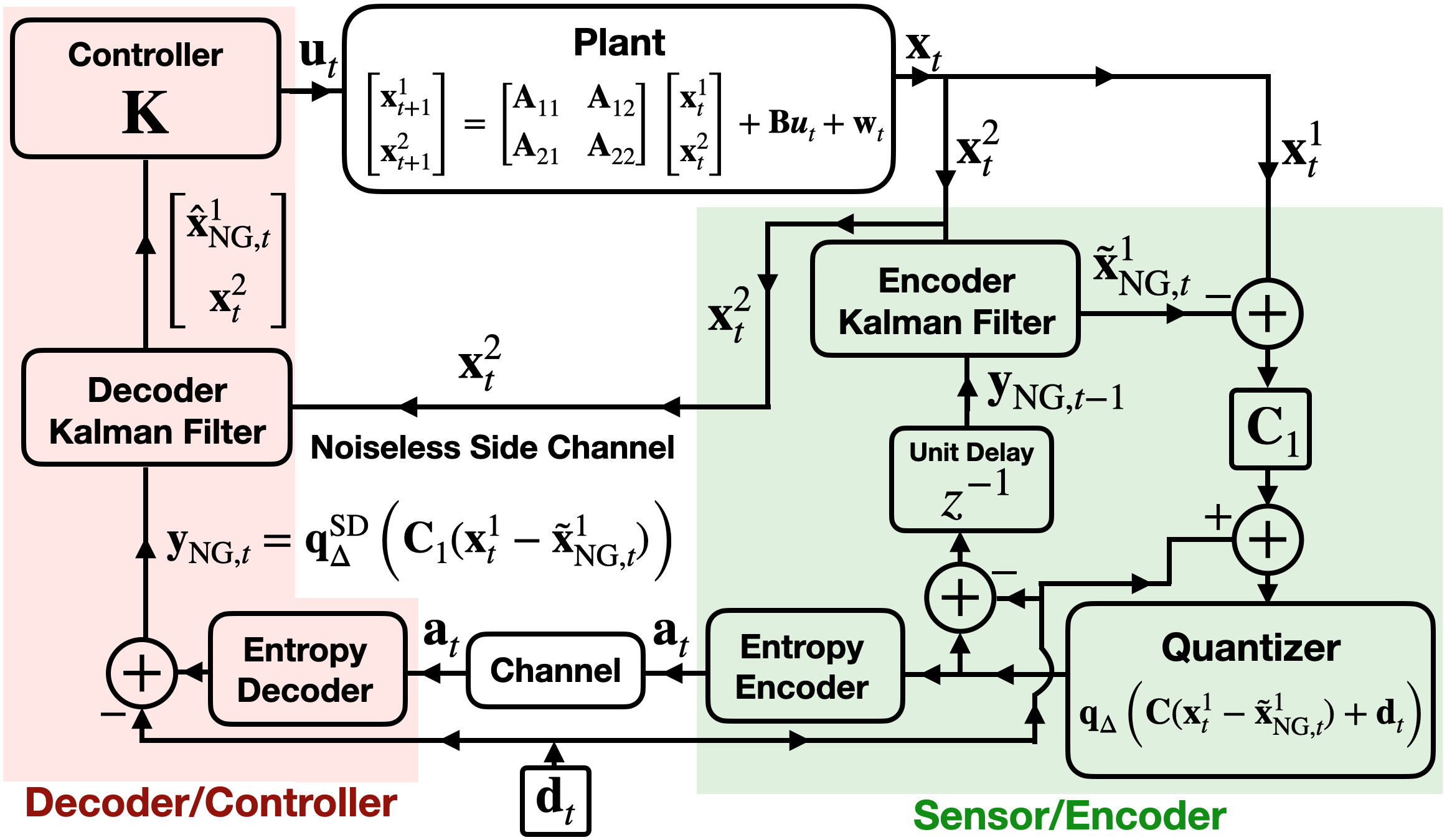
The architecture used to demonstrate the achievability result follows from [2, IV], and is shown in Fig. 4. As in [2], we use a predictive elementwise uniform quantizer with subtractive dither.

We define an elementwise uniform quantizer with sensitivity $\Delta$ as a function $\mathbf{q}_{\Delta}:\mathbb{R}^{n}\rightarrow\mathbb{R}^{n}$ such that

e.g. each element of $\mathbf{z}$ is “rounded" to the nearest integer multiple of $\Delta$. For a random input $\mathbf{z}$, $\mathbf{q}_{\Delta}(\mathbf{z})$ is a discrete RV with countable support. Consider the random vector $\mathbf{d}\in\mathbb{R}^{n}$ where $[\mathbf{d}]_{i}\sim\text{Uniform}[-\frac{\Delta}{2},\frac{\Delta}{2}]$ IID over $i$ and independent of $\mathbf{z}$. Define the quantizer with subtractive dither via

Dithering allows the quantization error to manifest as additive uniform noise; it can be shown that $\mathbf{n}=\mathbf{z}-\mathbf{q}^{\mathrm{SD}}_{\Delta}(\mathbf{z})$ is independent of $\mathbf{z}$ and that the elements $[\mathbf{n}]_{i}$ are IID with $[\mathbf{n}]_{i}\sim\text{Uniform}[-\frac{\Delta}{2},\frac{\Delta}{2}]$[2, Lemma 1a][13]. The caption of Fig. 4 outlines the use of dithering this achievability result.

We now show that when $\Delta=2\sqrt{3}$, the system in Fig. 4 achieves an equivalent control performance as the as the architecture in Fig. 2 for equivalent $\mathbf{C}_{1}$ and $\mathbf{V}=\mathbf{I}$. In Fig. 4, at time $t$ the decoder observes a dithered quantized measurement of $\mathbf{x}^{1}$, denoted $\mathbf{y}^{\mathrm{NG}}_{t}$ and to be described presently. The measurement is predictive and defined recursively via an encoder KF process. At time $t$, a KF at the encoder computes

The encoder’s quantizer computes the discrete $\mathbf{\tilde{z}}_{t}=\mathbf{q}_{\Delta}(\mathbf{C}_{1}(\mathbf{x}^{1}_{t}-\mathbf{\tilde{x}}^{1,\mathrm{NG}}_{t})+\mathbf{d}_{t})$, and encodes $\mathbf{\tilde{z}}_{t}$ with a prefix-free lossless Shannon-Fano-Elias (SFE) code. The codeword is sent to the decoder, which (exactly) reconstructs $\mathbf{\tilde{z}}_{t}$.

Given the dither signal, the decoder forms $\mathbf{y}^{\mathrm{NG}}_{t}=\mathbf{\tilde{z}}_{t}-\mathbf{d}_{t}$, or, equivalently $\mathbf{y}^{\mathrm{NG}}_{t}=\mathbf{q}_{\Delta}^{\mathrm{SD}}\left(\mathbf{C}_{1}(\mathbf{x}^{1}_{t}-\mathbf{\tilde{x}}^{1,\mathrm{NG}}_{t})\right)$. This gives

where $\mathbf{n}_{t}$ is a zero mean, uniform random vector with IID elements and $\mathbb{E}[\mathbf{n}_{t}\mathbf{n}_{t}^{\mathrm{T}}]=\mathbf{I}$. The decoder side Kalman filter operates analogously to the two stage filter in Fig. 3. Having received the previous measurements $\mathbf{y}^{\mathrm{NG}}_{1:t-1}$ and the SI $\mathbf{x}^{2}_{1:t}$, the decoder can compute $\mathbf{\tilde{x}}^{1,\mathrm{NG}}_{t}$ and form a centered measurement $\mathbf{\overline{y}}^{\mathrm{NG}}_{t}=\mathbf{y}^{\mathrm{NG}}_{t}+\mathbf{C}_{1}\mathbf{\tilde{x}}^{1,\mathrm{NG}}_{t}$. It clear that,

is the same as the LMMSE of $\mathbf{x}_{t}^{1}$ given $\mathbf{\overline{y}}^{\mathrm{NG}}_{1:t}$ and $\mathbf{x}^{2}_{1:t}$. The controller forms the control input $\mathbf{u}_{t}=\mathbf{K}[(\mathbf{\hat{x}}^{1,\mathrm{NG}}_{t})^{\mathrm{T}}\text{, }(\mathbf{{x}}_{t}^{2})^{\mathrm{T}}]^{\mathrm{T}}$ where $\mathbf{K}$ is as in (14). A corollary to the proof of [2, Lemma 1a] demonstrates that under this (really any) feedback arrangement, the sequence of quantization noises $\{\mathbf{n}_{t}\}$ is temporally white, e.g. $\mathbf{E}[\mathbf{n}_{t}\mathbf{n}_{t^{\prime}}^{\mathrm{T}}]=\mathbf{0}$ if $t\neq t^{\prime}$.

This leads to a result analogous to [2, Lemma 2]. Having fixed $\mathbf{C}_{1}$ and $\mathbf{V}=\mathbf{I}$, denote the jointly Gaussian random variables $(\mathbf{x}_{t},\mathbf{\tilde{x}}^{1}_{t},\mathbf{\hat{x}}^{1}_{t})$ with the joint distribution induced by the architecture in Fig. 2 by $(\mathbf{x}^{\mathrm{G}}_{t},\mathbf{\tilde{x}}^{1,\mathrm{G}}_{t},\mathbf{\hat{x}}^{1,\mathrm{G}}_{t})$. Likewise, denote the (generally non-Gaussian) RVs $(\mathbf{x}_{t},\mathbf{\tilde{x}}^{1}_{t},\mathbf{\hat{x}}^{1}_{t},)$ with the joint distribution induced by the architecture in Fig. 4 by $(\mathbf{x}^{\mathrm{NG}}_{t},\mathbf{\tilde{x}}^{1,\mathrm{NG}}_{t},\mathbf{\hat{x}}^{1,\mathrm{NG}}_{t})$. We have the following lemma.

It remains to bound the codeword length. Recall the discrete

Let $k=2+\frac{n}{2}\log_{2}\frac{4\pi e}{12}$. Our main result is the following.

References

• [1] T. Tanaka, P. M. Esfahani, and S. K. Mitter, “LQG control with minimum directed information: Semidefinite programming approach,” IEEE Trans. Automat. Contr., vol. 63, no. 1, pp. 37–52, 2018.
• [2] T. Tanaka, K. H. Johansson, T. Oechtering, H. Sandberg, and M. Skoglund, “Rate of prefix-free codes in LQG control systems,” in Proc. IEEE ISIT, 2016, pp. 2399–2403.
• [3] J. Massey, “Causality, feedback and directed information,” in Proc. IEEE ISIT, 1990, pp. 303–305.
• [4] O. Sabag, P. Tian, V. Kostina, and B. Hassibi, “The minimal directed information needed to improve the lqg cost,” in Proc. IEEE CDC, 2020, pp. 1842–1847.
• [5] E. I. Silva, M. S. Derpich, and J. Ostergaard, “A framework for control system design subject to average data-rate constraints,” IEEE Trans. Automat. Cont., vol. 56, no. 8, pp. 1886–1899, 2011.
• [6] V. Kostina and B. Hassibi, “Rate-cost tradeoffs in control,” IEEE Trans. on Automat. Cont., vol. 64, no. 11, pp. 4525–4540, 2019.
• [7] ——, “Rate-cost tradeoffs in scalar LQG control and tracking with side information,” in Proc. 56th Annu. Allerton Conf. on Commun., Control, and Comput., 2018, pp. 421–428.
• [8] P. A. Stavrou and M. Skoglund, “LQG control and linear policies for noisy communication links with synchronized side information at the decoder,” Automatica, vol. 123, p. 109306, 2021.
• [9] T. Cuvelier and T. Tanaka, “Rate of prefix-free codes in LQG control systems with side information,” arXiv preprint, 2021. [Online]. Available: https://arxiv.org/abs/2101.09329
• [10] T. M. Cover and J. A. Thomas, Elements of Information Theory. Wiley-Interscience, 1991.
• [11] T. Kailath, A. H. Sayed, and B. Hassibi, Linear Estimation. Prentice Hall, 2000.
• [12] S. Chan, G. Goodwin, and K. Sin, “Convergence properties of the Riccati difference equation in optimal filtering of nonstabilizable systems,” IEEE Trans. Automat. Contr., vol. 29, no. 2, pp. 110–118, 1984.
• [13] R. Zamir and M. Feder, “On universal quantization by randomized uniform/lattice quantizers,” IEEE Trans. Inf. Theory, vol. 38, no. 2, pp. 428 – 436, 1992.
Appendix A A formal proof of the converse bound
Refer to caption
Fig. 5: A generalized version of the path from encoder to decoder in the model of Fig. 1. The minimum achievable rate for a system with the additional “virtual" encoder/decoder pair lower bounds the minimum achievable rate for a system without the additional virtual pair.
Consider the system model in Fig. 1 at time tt. By assumption (cf. Sec. II), 𝐚t\mathbf{a}_{t} is a prefix-free codeword, so if 𝖺1≠𝖺2\mathsf{a}_{1}\neq\mathsf{a}_{2}, ℙ⁡(𝐚t=𝖺1)>0\mathbb{P}(\mathbf{a}_{t}=\mathsf{a}_{1})>0 and ℙ⁡(𝐚t=𝖺2)>0\mathbb{P}(\mathbf{a}_{t}=\mathsf{a}_{2})>0 then 𝖺1\mathsf{a}_{1} is not a prefix of 𝖺2\mathsf{a}_{2} and vice-versa. The codeword 𝐚t\mathbf{a}_{t} is a discrete variable with countable support chosen by the policy defined by kernel (a conditional PMF)
ℙS(𝐚t|𝐱1:t1,𝐱1:t2,𝐚1:t−1),\displaystyle\mathbb{P}_{S}(\mathbf{a}_{t}|\mathbf{x}^{1}_{1:t},\mathbf{x}^{2}_{1:t},\mathbf{a}_{1:t-1}), (42)
where we added the subscript SS to denote the “encoder/sensor" policy as in Fig 1. The control action is is chosen by the policy defined via the probability measure
ℙC(𝐮t|𝐚1:t,𝐱1:t2,𝐮1:t−1),\displaystyle\mathbb{P}_{C}(\mathbf{u}_{t}|\mathbf{a}_{1:t},\mathbf{x}^{2}_{1:t},\mathbf{u}_{1:t-1}), (43)
where we added the subscript CC to denote the “decoder/controller" policy as in Fig 1.
We bound the expected length of the prefix-free codeword 𝐚t\mathbf{a}_{t} at every tt by bounding the length of lossless prefix-free source code that encodes 𝐚t\mathbf{a}_{t} itself. Consider a modified version of the system model (cf. Fig. 1) shown in Fig. 5. Another, “virtual" encoder/decoder pair has been added between the encoder/sensor and decoder/controller. We assume that at every time tt, the virtual encoder encodes 𝐚t\mathbf{a}_{t} into a prefix-free codeword 𝐜t\mathbf{c}_{t}. We refer to 𝐚t\mathbf{a}_{t} as a “source codeword" and 𝐜t\mathbf{c}_{t} as a “virtual codeword". At every timestep tt, the virtual encoder encodes 𝐚t\mathbf{a}_{t} into the virtual codeword 𝐜t\mathbf{c}_{t} via computing
𝐜t=Ct​(𝐚t),\displaystyle\mathbf{c}_{t}=C_{t}(\mathbf{a}_{t}), (44)
for some deterministic measurable function CtC_{t}. Likewise, the virtual encoder computes the reconstruction 𝐚^t\mathbf{\hat{a}}_{t} by computing
𝐚^t=Dt​(𝐜t),\displaystyle\mathbf{\hat{a}}_{t}=D_{t}(\mathbf{c}_{t}), (45)
where again, for all tt, Dt{D}_{t} is a deterministic measurable function. The virtual encoder and decoder are both memoryless and do not access any SI. We insist that the virtual encoder and decoder are lossless, namely that 𝐚t​=a.s.​𝐚^t\mathbf{a}_{t}\overset{a.s.}{=}\mathbf{\hat{a}}_{t}. We think of Fig. 5 as “inserting" the virtual encoder and decoder blocks into Fig. 1. Note that virtual encoder and decoder policies do not effect the measure induced on the random variables 𝐱1:t,𝐚1:t,𝐮1:t\mathbf{x}_{1:t},\mathbf{a}_{1:t},\mathbf{u}_{1:t} due to the assumption that CtC_{t} and DtD_{t} are deterministic and that 𝐚^t​=a.s.​𝐚t\mathbf{\hat{a}}_{t}\overset{a.s.}{=}\mathbf{a}_{t}.
The idea is that the insertion of an optimal “virtual" lossless encoder/decoder between the sensor and controller produces a codeword ctc_{t} that has a length less than or equal to that of 𝐚t\mathbf{a}_{t}. More formally, at every time tt we lower bound the length of the codeword 𝐚t\mathbf{a}_{t} by lower bounding the length of the codeword 𝐜t\mathbf{c}_{t} under the optimal zero-error prefix free virtual encoder and virtual decoder policies. If 𝐫\mathbf{r} is a prefix free binary codeword, let ℓ⁡(𝐫)\ell(\mathbf{r}) denote its length. An “optimal" virtual encoder and decoder policy (there may be more than one), for some fixed sensor and controller policy, is defined as a sequence of deterministic functions P∗={Ct∗,Dt∗}P^{*}=\{{C}^{*}_{t},{D}^{*}_{t}\} where:
1. 1.
Ct∗{C}^{*}_{t} maps 𝐚t\mathbf{a}_{t} to 𝐜t\mathbf{c}_{t} and Dt∗{D}^{*}_{t} maps 𝐜t\mathbf{c}_{t} to 𝐚^t\mathbf{\hat{a}}_{t} as in Fig. 5.
2. 2.
There is no probability of error, e.g. Dt∗​(Ct∗​(𝐚t))​=a.s.​𝐚tD^{*}_{t}(C^{*}_{t}(\mathbf{a}_{t}))\overset{a.s.}{=}\mathbf{a}_{t} for all tt.
3. 3.
Let 𝒜t={𝖺∈{0,1}∗:ℙ⁡(𝐚t=𝖺)>0}\mathcal{A}_{t}=\{\mathsf{a}\in\{0,1\}^{*}:\mathbb{P}(\mathbf{a}_{t}=\mathsf{a})>0\}. At every time tt, if 𝖺1,𝖺2∈𝒜t\mathsf{a}_{1},\mathsf{a}_{2}\in\mathcal{A}_{t} and 𝖺1≠𝖺2\mathsf{a}_{1}\neq\mathsf{a}_{2} then 𝖼1=Ct∗​(𝖺1)\mathsf{c}_{1}=C^{*}_{t}(\mathsf{a}_{1}) is not a prefix of 𝖼2=Ct∗​(𝖺2)\mathsf{c}_{2}=C^{*}_{t}(\mathsf{a}_{2}) and vice-versa.22 2 This ensures that Ct∗C^{*}_{t}, restricted to 𝒜t\mathcal{A}_{t} is injective; a necessary condition for there to exist a deterministic Dt∗D^{*}_{t} such that Dt∗​(Ct∗​(𝐚t))​=a.s.​𝐚tD^{*}_{t}(C^{*}_{t}(\mathbf{a}_{t}))\overset{a.s.}{=}\mathbf{a}_{t} (cf. condition (2)). It also ensures that the set of virtual codewords transmitted with nonzero probability at time tt are not prefixes of one another; define 𝒞t∗={𝐜∈{0,1}∗:ℙ⁡(Ct​(𝐚t)=𝐜)>0}\mathcal{C}^{*}_{t}=\{\mathbf{c}\in\{0,1\}^{*}:\mathbb{P}(C_{t}(\mathbf{a}_{t})=\mathbf{c})>0\}, and let 𝖼1,𝖼2∈𝒞t\mathsf{c}_{1},\mathsf{c}_{2}\in\mathcal{C}_{t}. If 𝖼1≠𝖼2\mathsf{c}_{1}\neq\mathsf{c}_{2}, then 𝖼1\mathsf{c}_{1} is not a prefix of 𝖼2\mathsf{c}_{2} and vice-versa.
4. 4.
At all tt, 𝔼⁡[ℓ⁡(𝐜t)]\mathbb{E}[\ell(\mathbf{c}_{t})] is minimized among all other policies satisfying (1), (2), and (3) above.
The above expectations and probabilities are taken with respect to the measure induced by the sensor and controller policies ℙS\mathbb{P}_{S} and ℙC\mathbb{P}_{C} and Fig. 1. In the language of [10, Chapter 5], the constraints (1), (2), and (3) require that at any time tt, Ct∗C^{*}_{t} is prefix-free code mapping the space 𝒜t⊂{0,1}∗\mathcal{A}_{t}\subset\{0,1\}^{*} to the space of binary prefix-free codewords in {0,1}∗\{0,1\}^{*}. In the next lemma, we show that under the optimal virtual encoder and decoder policies, we have
𝔼⁡[ℓ⁡(Ct∗​(𝐚t))]≤𝔼⁡[ℓ⁡(𝐚t)],\displaystyle\mathbb{E}[\ell(C^{*}_{t}(\mathbf{a}_{t}))]\leq\mathbb{E}[\ell(\mathbf{a}_{t})], (46a)
or, in other words
𝔼⁡[ℓ⁡(𝐜t)]≤𝔼⁡[ℓ⁡(𝐚t)],\displaystyle\mathbb{E}[\ell(\mathbf{c}_{t})]\leq\mathbb{E}[\ell(\mathbf{a}_{t})], (46b)
where 𝐜t=Ct∗​(𝐚t)\mathbf{c}_{t}=C^{*}_{t}(\mathbf{a}_{t}).
Lemma A.1.
For all tt there exists a CtC_{t} and DtD_{t} satisfying (1)-(4) above and 𝔼⁡[ℓ⁡(𝐜t)]≤𝔼⁡[ℓ⁡(𝐚t)]\mathbb{E}[\ell(\mathbf{c}_{t})]\leq\mathbb{E}[\ell(\mathbf{a}_{t})].
Proof.
At every time tt, the source codewords 𝐚t\mathbf{a}_{t} are codewords of a prefix-free code. Setting CtC_{t} and DtD_{t} equal to identity, e.g.
𝐚t=Ct​(𝐚t)\displaystyle\mathbf{a}_{t}=C_{t}(\mathbf{a}_{t}) and ​𝐜t=Ct​(𝐜t),\displaystyle\text{ and }\mathbf{c}_{t}=C_{t}(\mathbf{c}_{t}), (47)
gives
𝐜t=𝐚t\displaystyle\mathbf{c}_{t}=\mathbf{a}_{t} and ​𝐚^t=𝐜t\displaystyle\text{ and }\mathbf{\hat{a}}_{t}=\mathbf{c}_{t} (48)
Under this policy, the virtual encoder sends the input 𝐚t\mathbf{a}_{t} directly and 𝐚t=𝐜t=𝐚^t\mathbf{a}_{t}=\mathbf{c}_{t}=\mathbf{\hat{a}}_{t}. Thus there exist policies satisfying the constraints that achieve equality in (46) and the result follows. ∎
Since for every tt, Ct∗C^{*}_{t} is a prefix-free code from 𝒜t→{0,1}∗\mathcal{A}_{t}\rightarrow\{0,1\}^{*}, it follows from [10, Theorem 5.3.1] that
H⁡(𝐚t)≤𝔼⁡[ℓ⁡(Ct∗​(𝐚t))],\displaystyle H(\mathbf{a}_{t})\leq\mathbb{E}[\ell(C^{*}_{t}(\mathbf{a}_{t}))], (49)
which gives the result
H⁡(𝐚t)≤𝔼⁡[ℓ⁡(𝐚t)].\displaystyle H(\mathbf{a}_{t})\leq\mathbb{E}[\ell(\mathbf{a}_{t})]. (50)
We emphasize that (50) holds for every time tt.
Appendix B Proof of equivalence between (30) and (31)
We begin by writing (30) in terms of 𝐏^\mathbf{\hat{P}} only. It can immediately be seen that the design variables 𝐂\mathbf{C} and 𝐕\mathbf{V} are essentially slack. The constraint 𝐏^−1=𝐏~−1+𝐂1T​𝐕−1​𝐂1\mathbf{\hat{P}}^{-1}=\mathbf{\tilde{P}}^{-1}+\mathbf{C}_{1}^{\mathrm{T}}\mathbf{V}^{-1}\mathbf{C}_{1} can be replaced with the constraints 𝐏~−𝐏^⪰𝟎\mathbf{\tilde{P}}-\mathbf{\hat{P}}\succeq\mathbf{0} and 𝐏^≻𝟎\mathbf{\hat{P}}\succ\mathbf{0}. The new inequality constraint may be readily combined with the equality constraint for 𝐏~\mathbf{\tilde{P}} (cf. (27b)) to derive a linear matrix inequality (LMI) in 𝐏^\mathbf{\hat{P}}. Applying the matrix inversion lemma to (27b) gives
𝐏~−𝐏^=𝐖11−𝐏^+𝐀11​(𝐏^−𝐏^​𝐀21T​(𝐀21​𝐏^​𝐀21T+𝐖22)−1​𝐀21​𝐏^)​𝐀11T.\mathbf{\tilde{P}}-\mathbf{\hat{P}}=\mathbf{W}_{11}-\mathbf{\hat{P}}+\\ \mathbf{A}_{11}\left(\mathbf{\hat{P}}-\mathbf{\hat{P}}\mathbf{A}_{21}^{\mathrm{T}}(\mathbf{A}_{21}\mathbf{\hat{P}}\mathbf{A}_{21}^{\mathrm{T}}+\mathbf{W}_{22})^{-1}\mathbf{A}_{21}\mathbf{\hat{P}}\right)\mathbf{A}_{11}^{\mathrm{T}}. (51)
The right hand side of (51) is a Shur complement, and the LMI constraint follows directly. Thus 𝐏~−𝐏^⪰0\mathbf{\tilde{P}}-\mathbf{\hat{P}}\succeq 0 is equivalent to the LMI
𝐖+𝐀¯​𝐏^​𝐀¯T−[𝐏^000]⪰0.\displaystyle\mathbf{W}+\mathbf{\bar{A}}\mathbf{\hat{P}}\mathbf{\bar{A}}^{\mathrm{T}}-\begin{bmatrix}\mathbf{\hat{P}}&0\\ 0&0\end{bmatrix}\succeq 0. (52)
The corresponding 𝐂1\mathbf{C}_{1} and 𝐕\mathbf{V} are not unique, and can be found by factorizing 𝐏^−1−𝐏~−1\mathbf{\hat{P}}^{-1}-\mathbf{\tilde{P}}^{-1}.
It remains to simplify the rate cost. Using (27b) and invoking the matrix determinant lemma twice, we
logdet𝐏~−logdet𝐏^=logdet(𝐏^−1+𝐀¯T𝐖−1𝐀¯)+logdet𝐖−logdet(𝐖22+𝐀21𝐏^𝐀21T).\log\det\mathbf{\tilde{P}}-\log\det\mathbf{\hat{P}}=\log\det(\mathbf{\hat{P}}^{-1}+\mathbf{\bar{A}}^{\mathrm{T}}\mathbf{W}^{-1}\mathbf{\bar{A}})+\\ \log\det\mathbf{W}-\log\det(\mathbf{W}_{22}+\mathbf{A}_{21}\mathbf{\hat{P}}\mathbf{A}_{21}^{\mathrm{T}}). (53)
Introduce the slack variable 𝚷\boldsymbol{\Pi}. We have
logdet(𝐏^−1+𝐀¯T𝐖−1𝐀¯)=min0⪯𝚷⪯(𝐏^−1+𝐀¯T​𝐖−1​𝐀¯)−1−logdet𝚷.\log\det(\mathbf{\hat{P}}^{-1}+\mathbf{\bar{A}}^{\mathrm{T}}\mathbf{W}^{-1}\mathbf{\bar{A}})=\\ \min_{0\preceq\boldsymbol{\Pi}\preceq(\mathbf{\hat{P}}^{-1}+\mathbf{\bar{A}}^{\mathrm{T}}\mathbf{W}^{-1}\mathbf{\bar{A}})^{-1}}-\log\det\boldsymbol{\Pi}. (54)
Applying the matrix inversion lemma and the Shur complement formula to the constraint 𝚷⪯(𝐏^−1+𝐀¯T​𝐖−1​𝐀¯)−1\boldsymbol{\Pi}\preceq(\mathbf{\hat{P}}^{-1}+\mathbf{\bar{A}}^{\mathrm{T}}\mathbf{W}^{-1}\mathbf{\bar{A}})^{-1} gives the equivalent LMI
[𝐏^−𝚷𝐏^​𝐀¯T𝐀¯​𝐏^𝐖+𝐀¯​𝐏^​𝐀¯T]⪰0.\displaystyle\begin{bmatrix}\mathbf{\hat{P}}-\boldsymbol{\Pi}&\mathbf{\hat{P}}\mathbf{\bar{A}}^{\mathrm{T}}\\ \mathbf{\bar{A}}\mathbf{\hat{P}}&\mathbf{W}+\mathbf{\bar{A}}\mathbf{\hat{P}}\mathbf{\bar{A}}^{\mathrm{T}}\end{bmatrix}\succeq 0. (55)
The preceding discussion demonstrates that
min𝐏^,𝚷logdet𝐖−logdet𝚷−logdet(𝐖22+𝐀21𝐏^𝐀21T)2\displaystyle\underset{\displaystyle\mathbf{\hat{P}},\boldsymbol{\Pi}}{\mathrm{min}}\quad\frac{\log\det\mathbf{W}-\log\det\boldsymbol{\Pi}-\log\det{(\mathbf{W}_{22}+\mathbf{A}_{21}\mathbf{\hat{P}}\mathbf{A}_{21}^{\mathrm{T}})}}{2}\hfil\hfil\displaystyle\displaystyle\hfil\hfil\displaystyle\displaystyle (56)
s.t.\displaystyle\mathmakebox[\widthof{$\underset{\displaystyle\phantom{\mathbf{\hat{P}},\boldsymbol{\Pi}}}{\mathrm{min}}$}][c]{\mathmakebox[\widthof{$\mathrm{min}$}][l]{\mathrm{\kern 1.00006pts.t.}}}\quad 𝐏^≻0,𝚷⪰0,Tr(𝚯𝐏^)+Tr(𝐒𝐖)≤γ,\displaystyle\mathbf{\hat{P}}\succ{0},\boldsymbol{\Pi}\succeq 0,\text{Tr}(\mathbf{\Theta}\mathbf{\hat{P}})+\text{Tr}(\mathbf{S}\mathbf{W})\leq\gamma,\hfil\hfil\displaystyle\displaystyle
𝐖+𝐀¯​𝐏^​𝐀¯T−[𝐏^000]⪰0,\displaystyle\mathbf{W}+\mathbf{\bar{A}}\mathbf{\hat{P}}\mathbf{\bar{A}}^{\mathrm{T}}-\begin{bmatrix}\mathbf{\hat{P}}&0\\ 0&0\end{bmatrix}\succeq 0,\hfil\hfil\displaystyle\displaystyle
[𝐏^−𝚷𝐏^​𝐀¯T𝐀¯​𝐏^𝐖+𝐀¯​𝐏^​𝐀¯T]⪰0.\displaystyle\begin{bmatrix}\mathbf{\hat{P}}-\boldsymbol{\Pi}&\mathbf{\hat{P}}\mathbf{\bar{A}}^{\mathrm{T}}\\ \mathbf{\bar{A}}\mathbf{\hat{P}}&\mathbf{W}+\mathbf{\bar{A}}\mathbf{\hat{P}}\mathbf{\bar{A}}^{\mathrm{T}}\end{bmatrix}\succeq 0.
achieves the same minimum as (30). This program is the minimization of a convex objective with convex constraints.
Appendix C Proof of Lemma VI.2
The proof follows closely from [2]. Assume the definitions of Sec. VI. It turns out that H⁡(𝐳~t|𝐝t)H(\mathbf{\tilde{z}}_{t}|\mathbf{d}_{t}) admits a bound in terms of the squared error rate distortion function of 𝐳\mathbf{z} [2, Lemma 1 c-d]. Let D=n​Δ2/12=nD={n\Delta^{2}/12}=n. Define the rate distortion function
ℛ𝐱(D)=infℙ⁡(𝐮|𝐱):𝔼⁡[∥𝐱−𝐮∥22]≤DI(𝐱;𝐮).\displaystyle\mathcal{R}_{\mathbf{x}}(D)=\underset{\mathbb{P}(\mathbf{u}|\mathbf{x}):\mathbb{E}[\lVert\mathbf{x}-\mathbf{u}\rVert_{2}^{2}]\leq D}{\inf}I(\mathbf{x};\mathbf{u}). (57)
We have
H⁡(𝐳~t|𝐝t)≤n2​log2​4​π​e12+ℛ𝐳t​(D).\displaystyle H(\mathbf{\tilde{z}}_{t}|\mathbf{d}_{t})\leq\frac{n}{2}\log_{2}\frac{4\pi e}{12}+\mathcal{R}_{\mathbf{z}_{t}}(D). (58)
It is known (cf. [10, Problem 10.8]) that if a Gaussian random vector 𝐱\mathbf{x} has cov​(𝐱)=cov​(𝐳)\text{cov}(\mathbf{x})=\text{cov}(\mathbf{z}) then ℛ𝐳​(D)≤ℛ𝐱​(D)\mathcal{R}_{\mathbf{z}}(D)\leq\mathcal{R}_{\mathbf{{x}}}(D).
We claim that
ℛ𝐳t​(D)≤I⁡(𝐂1​𝐫~tG,𝐂1​𝐫~tG+𝐯t)\displaystyle\mathcal{R}_{\mathbf{z}_{t}}(D)\leq I(\mathbf{C}_{1}\mathbf{\tilde{r}}^{\mathrm{G}}_{t};\mathbf{C}_{1}\mathbf{\tilde{r}}^{\mathrm{G}}_{t}+\mathbf{v}_{t}) (59)
Note that 𝚯t=𝐂1​𝐫~tG\boldsymbol{\Theta}_{t}=\mathbf{C}_{1}\mathbf{\tilde{r}}^{\mathrm{G}}_{t} is Gaussian and that, by Lemma VI.1 we have 𝔼⁡[𝚯t​𝚯tT]=𝔼⁡[𝐳t​𝐳tT]=𝐂1​𝐏~t​𝐂1T\mathbb{E}[\boldsymbol{\Theta}_{t}\boldsymbol{\Theta}_{t}^{\mathrm{T}}]=\mathbb{E}[\mathbf{z}_{t}\mathbf{z}_{t}^{\mathrm{T}}]=\mathbf{C}_{1}\mathbf{\tilde{P}}_{t}\mathbf{C}_{1}^{\mathrm{T}} and that 𝔼⁡[𝚯t]=𝔼⁡[𝐳t]=𝟎\mathbb{E}[\boldsymbol{\Theta}_{t}]=\mathbb{E}[\mathbf{z}_{t}]=\mathbf{0}. Thus ℛ𝐳t​(D)≤ℛ𝚯t​(D)\mathcal{R}_{\mathbf{z}_{t}}(D)\leq\mathcal{R}_{\boldsymbol{\Theta}_{t}}(D). By the assumption that 𝐕=𝐈\mathbf{V}=\mathbf{I}, we have 𝔼⁡[𝐯tT​𝐯t]=n\mathbb{E}[\mathbf{v}^{\mathrm{T}}_{t}\mathbf{v}_{t}]=n. Since D=nD=n, ℛ𝚯t​(D)≤I⁡(𝐂1​𝐫~tG,𝐂1​𝐫~tG+𝐯t)\mathcal{R}_{\boldsymbol{\Theta}_{t}}(D)\leq I(\mathbf{C}_{1}\mathbf{\tilde{r}}^{\mathrm{G}}_{t};\mathbf{C}_{1}\mathbf{\tilde{r}}^{\mathrm{G}}_{t}+\mathbf{v}_{t}), and (59) follows. Substituting this into this into (58) establishes the Lemma.