High-efficient two-step entanglement purification using hyperentanglement

Entanglement is an indispensable resource which is widely applied in quantum communication field, such as quantum teleportationteleportation1; teleportation2; teleportation3, quantum repeater repeater1; repeater2; repeater3, quantum key distribution (QKD) qkd, quantum secret sharing (QSS) qss, and quantum secure direct communication (QSDC) qsdc1; qsdc2; qsdc3; qsdc4. The above applications often require the maximal entanglement. However, entanglement is generally fragile due to the channel noise. During the practical applications, the degraded entanglement may decrease the quantum communication efficiency or even make quantum communication insecure.

Entanglement purification which was first proposed by Bennett et al. in 1996 EPP0 is an efficient method to distill high quality entanglement from low quality entanglement with local operation and classical communications (LOCC). Recurrence entanglement purification is the most common entanglement purification form, which has been well developed in both theory and experiment EPP0; Deustch; Murao; Pan1; Pan2; Pan3; graph; atom; Cheong; sheng1; sheng2; Zhou1; Wang; Zhou2; Zhang; Dur; Rozpeedek; Krastanov; Wu; zhouap; zhouoe; hu; Du; nest; network; shenghyper1; shenghyper2. The recurrence entanglement purification protocols (EPPs) require two or more copies of low-quality entangled states from the same enables. After two communication parties in distant locations performing the controlled-not (CNOT) or other similar operations, one pair of low-quality entangled state is measured. If the purification is successful, the fidelity of left photon pair can be increased. For example, in 2001, Pan et al. presented an EPP of general mixed entangled states with linear optical elements Pan1, and later they improved their EPP by adopting available parametric down conversion sources Pan2. In 2003, Pan et al. demonstrated the experiment of the entanglement purification for general mixed states of polarization-entangled photons Pan3. In 2008, Sheng et al. proposed an EPP based on nondestructive quantum nondemolition detectors sheng1. In 2017, Pan et al. experimentally realized the nested purification for a linear optical quantum repeater nest. In addition, the experimental purification between two-atom entanglement and solid state quantum network nodes were also demonstrated atom; network. In 2010, Sheng et al. proposed the deterministic EPPs (DEPPs) by adopting the hyperentanglement shenghyper1; shenghyper2.

Although the recurrence entanglement purification has been well studied, existing recurrence EPPs often have relatively low yield. The reason is that in each purification round, at least one pair of low-quality entangled states should be consumed. In practical applications, entanglement purification process often has to be iterated for many rounds to obtain high-fidelity entangled pairs, so that a large amount of low-quality entangled pairs have to be consumed. It is a big waste of the precious entanglement resources. In 2021, Hu et al. proposed and experimentally demonstrated the first long-distance polarization entanglement recurrence purification using only one polarization-spatial-mode hyperentangled photon pair hu. They supposed that the entanglement in both polarization and spatial-mode DOFs suffer from one kind of error, say, the bit-flip error or phase-flip error. After performing the EPP, they obtained a significant improvement in the fidelity of polarization entanglement. This protocol effectively reduces consumption of copies of entanglement pairs, especially in purification consisting of many rounds.

Actually, in practical entanglement distribution process, the bit-flip error and phase-flip error may be occurred simultaneously. In the paper, we consider a more general recurrence EPP which can simultaneously reduce the bit-flip error and phase-flip error of the polarization entanglement by using only one pair of polarization-spatial-time-bin hyperentangled photon pair. We choose the spatial mode and time-bin entanglement for the entanglement in both two DOFs, especially in time-bin DOF being highly robust to the channel noise. The entanglement in time-bin DOF has been successfully used in the transmission of qubits over hundreds of kilometers Pan2; time1; time2; time3; time4 and in teleportation using real-world fiber networks time5; time6. In 2005, Barreiro et al. experimentally demonstrated the generation of hyperentanglement in polarization, spatial-mode and time-energy DOFs of photon systems using pairs of photons produced in spontaneous parametric down-conversion generation5. In our protocol, we suppose that the entanglement in all DOFs suffer from channel noise and degrade to mixed states. As the entanglement in above three DOFs have different noise robustness, after the photon transmission, the fidelities in three DOFs are naturally different. After performing our EPP, we can efficiently reduce both the bit-flip error and phase-flip error rate in polarization DOF by consuming the imperfect entanglement in the spatial-mode and time-bin DOFs. Moreover, we will prove that if a purification step fails, there may exist residual entanglement in the corresponding distilled mixed state. By using the residual entanglement, we may also increase the fidelity of the polarization entanglement after the whole purification process.

The paper is organized as follows. In Sec. II, we describe our EPP in a simple case where the entanglement in spatial-mode and time-bin DOFs only suffer from a bit-flip error. In Sec. III, we extend our EPP to a general case where both the entanglement in spatial-mode and time-bin DOFs suffer from both bit-flip error and phase-flip error. In Sec. IV, we make a discussion. In Sec. V, we make a conclusion.

In this section, we propose our long-distance EPP using a hyperentangled photon pair. Suppose the photon hyperentanglement source S generates a two-photon hyperentanglement in polarization, spatial-mode, and time-bin DOFs, which can be described as

Here, $H$ ($V$) represents the horizontal (vertical) polarization, $a_{1}^{\prime}$, $a_{2}^{\prime}$, $b_{1}^{\prime}$ and $b_{2}^{\prime}$ are four different spatial modes, and $L$ ($S$) represents the long (short) time-bin.

The photon in $a_{1}^{\prime}$ and $a_{2}^{\prime}$ are sent to Alice, while the photon in $b_{1}^{\prime}$ and $b_{2}^{\prime}$ are sent to Bob. After long distance transmission, the channel noise may degrade the entanglement in all DOFs. Here, we suppose that the entanglement in polarization DOF degrade to a Werner state with the form of

where

We notice that the state $|\Phi^{+}_{p}\rangle$ becomes $|\Psi^{+}_{p}\rangle$ when a bit-flip error occurs, $|\Phi^{+}_{p}\rangle$ becomes $|\Phi^{-}_{p}\rangle$ when a phase-flip error occurs, and $|\Phi^{+}_{p}\rangle$ becomes $|\Psi^{-}_{p}\rangle$ when bit-flip error and phase-flip error both occur.

Considering the noise robustness of the entanglement in spatial-mode and time-bin DOFs are higher than that in the polarization DOF, we first focus on a simple case where the entanglement in spatial-mode and time-bin DOFs only suffer from bit-flip error. In this case, the entanglement in both DOFs degrade to

where

Therefore, the initial state in Eq. (1) degrades to $\rho_{p}\otimes\rho_{s}\otimes\rho_{t}$. Here, we suppose that all the fidelity $p_{p}$, $p_{s}$, and $p_{t}$ are higher than $\frac{1}{2}$. The schematic principle of our EPP is shown in Fig. 1. The protocol includes two steps. In the first step, Alice and Bob correct the bit-flip error in polarization DOF by consuming the entanglement in spatial-mode DOF. In the second step, they correct the phase-flip error in polarization DOF with the help of the entanglement in time-bin DOF.

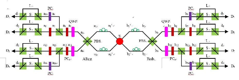
In the first step, we only use the states in polarization and spatial-mode DOF and leave the state in time-bin DOF unchanged, so that we first neglect the state in time-bin DOF and only consider the mixed state as $\rho_{1}=\rho_{p}\otimes\rho_{s}$ for simplicity. There are totally eight possible cases. The photon system may be in $|\Phi^{+}_{p}\rangle|\Phi^{+}_{s}\rangle$ with the probability of $p_{p}p_{s}$, while it may be in $|\Phi^{+}_{p}\rangle|\Psi^{+}_{s}\rangle$ with the probability of $p_{p}(1-p_{s})$. Meanwhile, the photon system may be in $|\Psi^{+}_{p}\rangle|\Phi^{+}_{s}\rangle$, $|\Phi^{-}_{p}\rangle|\Phi^{+}_{s}\rangle$, or $|\Psi^{-}_{p}\rangle|\Phi^{+}_{s}\rangle$ with the equal probability of $\frac{(1-p_{p})p_{s}}{3}$, and it may be in the state $|\Psi^{+}_{p}\rangle|\Psi^{+}_{s}\rangle$, $|\Phi^{-}_{p}\rangle|\Psi^{+}_{s}\rangle$, or $|\Psi^{-}_{p}\rangle|\Psi^{+}_{s}\rangle$ with the probability of $\frac{(1-p_{p})(1-p_{s})}{3}$.

Alice and Bob pass the photons in $a_{1}$ and $a_{2}$, $b_{1}$ and $b_{2}$ spatial modes through two polarization beam splitters (PBSs), which can totally transmit the photon in $|H\rangle$ and reflect the photon in $|V\rangle$. If the initial photon state is $|\Phi^{\pm}_{p}\rangle|\Phi^{+}_{s}\rangle$, after the PBS, the state will evolve to

When the initial state is $|\Psi^{\pm}_{p}\rangle|\Psi^{+}_{s}\rangle$, it will evolve to

All the four above states make the spatial modes $a_{3}b_{3}$ or $a_{4}b_{4}$ each have one photon. In these cases, the first step is successful. On the other hand, if the initial state is one of the other four cases, say, $|\Phi^{\pm}_{p}\rangle|\Psi^{+}_{s}\rangle$ and $|\Psi^{\pm}_{p}\rangle|\Phi^{+}_{s}\rangle$, after the PBSs, we can obtain the spatial-modes $a_{3}b_{4}$ or $a_{4}b_{3}$ each has one photon and the first step fails.

As a result, when the first step is successful, we can distill a new mixed state as

in the spatial modes $a_{3}b_{3}$ or $a_{4}b_{4}$ with the success probability of

The four coefficients in Eq. (9) can be written as

It is obvious that when $p_{p}>\frac{1}{2}$ and $p_{s}>\frac{1}{2}$, the rate of $|\Psi^{\pm}_{p}\rangle$ ($F_{3}$) is smaller than their original rate $\frac{(1-p_{p})}{3}$. As a result, the first step can reduce the rate of $|\Psi^{\pm}_{p}\rangle$. Moreover, the reduction of bit-flip error directly increases the fidelity of $|\Phi^{+}_{p}\rangle$. We can obtain $F_{1}>p_{p}$ and $F_{1}>p_{s}$ when $p_{p}>\frac{1}{2}$ and $\frac{5p_{p}-2}{4p_{p}-1}>p_{s}>\frac{1}{2}$. However, the first step cannot deal with the phase-flip error ($|\Phi^{-}_{p}\rangle$) and the rate of $|\Phi^{-}_{p}\rangle$ is still in a relatively high level. Next, we try to correct the phase-flip error.

In the second step, we require to consume the entanglement in the time-bin DOF. After the first step, the whole photon system collapse to $\rho_{1p}\otimes\rho_{t}$ in $a_{3}b_{3}$ or $a_{4}b_{4}$ modes. We first consider that the photons are in $a_{3}b_{3}$. Alice and Bob first pass the photons in $a_{3}b_{3}$ modes through two $\lambda/4$-wave plates (QWPs), respectively. The QWP performs a Hadamard (H) operation in the polarization DOF, which makes $|H\rangle\rightarrow\frac{1}{\sqrt{2}}(|H\rangle+|V\rangle)$ and $|V\rangle\rightarrow\frac{1}{\sqrt{2}}(|H\rangle-|V\rangle)$. After the H operation, $|\Phi^{-}_{p}\rangle\leftrightarrow|\Psi^{+}_{p}\rangle$, while $|\Phi^{+}_{p}\rangle$ and $|\Psi^{-}_{p}\rangle$ keep unchanged. In this way, they can transform $\rho_{1p}$ to

in the spatial modes $a_{5}b_{5}$. The whole photon system $\rho_{2p}\otimes\rho_{t}$ can be described as follows. With probability of $F_{1}p_{t}$ and $F_{1}(1-p_{t})$ the photon pair is in $|\Phi^{+}_{p}\rangle|\Phi^{+}_{t}\rangle$ and $|\Phi^{+}_{p}\rangle|\Psi^{+}_{t}\rangle$, respectively. With a probability of $F_{2}p_{t}$ and $F_{2}(1-p_{t})$, it is in $|\Psi^{+}_{p}\rangle|\Phi^{+}_{t}\rangle$ and $|\Psi^{+}_{p}\rangle|\Psi^{+}_{t}\rangle$, respectively. On the other hand, the whole system is in $|\Phi^{-}_{p}\rangle|\Phi^{+}_{t}\rangle$ or $|\Psi^{-}_{p}\rangle|\Phi^{+}_{t}\rangle$ with an equal probability of $F_{3}p_{t}$, and in $|\Phi^{-}_{p}\rangle|\Psi^{+}_{t}\rangle$ or $|\Psi^{-}_{p}\rangle|\Psi^{+}_{t}\rangle$ with an equal probability of $F_{3}(1-p_{t})$.

Suppose that the photon pair is in $|\Phi^{+}_{p}\rangle_{a_{5}b_{5}}|\Phi^{+}_{t}\rangle$. As shown in Fig. 1, Alice (Bob) passes the photon in $a_{5}$ $(b_{5})$ through a Pockels cell ($PC_{S}$), which can flip the polarization feature of the incoming photon under the temporal mode $S$. After the $PC_{s}$, Alice (Bob) passes the photon through a PBS, which makes the photon in $|H\rangle$ be in $a_{7}$ $(b_{7})$ and enter a $PC_{S}$ and the photon in $|V\rangle$ be in $a_{8}$ $(b_{8})$ and enter a $PC_{L}$. As a result, the states $|\Phi^{\pm}_{p}\rangle|\Phi^{+}_{t}\rangle$ will finally evolve to

Then, with the help of two PBSs, Alice and Bob can make the photon in $|H\rangle$ pass through the short (S) arm and photon in $|V\rangle$ pass through the long (L) arm. By precisely controlling the length of long and short arms, they can adjust the time-bin feature of the photons in $|H\rangle$ and $|V\rangle$ to be the same. In this way, we can neglect the time-bin features of the photons, and the state in Eq. (13) evolves to

and will be detected by the single photon detector $D_{2}D_{6}$ or $D_{1}D_{5}$. In this case, the second purification step is successful. The polarization feature of the photon pair remains to be $|\Phi^{\pm}_{p}\rangle$.

If the initial state is $|\Psi^{\pm}_{p}\rangle|\Psi^{+}_{t}\rangle$, after the above operations, it will evolve to

which will also lead to the successful detection results. The state in Eq. (15) will finally collapse to $|\Psi^{\pm}_{p}\rangle$.

If the initial state is $|\Phi^{\pm}_{p}\rangle|\Psi^{+}_{t}\rangle$ or $|\Psi^{\pm}_{p}\rangle|\Phi^{+}_{t}\rangle$, after the above operations, Alice and Bob would never obtain the successful measurement results. In detail, after above operations, we can obtain

which makes the single photon detectors $D_{1}D_{6}$ or $D_{2}D_{5}$ each register a single photon. In this case, the second purification step fails.

On the other hand, if the photon state is in $a_{4}b_{4}$ modes, we can obtain when the photon detectors $D_{3}D_{7}$ or $D_{4}D_{8}$ each register one photon, the second purification step is successful.

Therefore, when the second purification step is successful, we can distill a new mixed state in polarization DOF as

with a success probability of

The four coefficients in Eq. (17) can be written as

Similarly as the first step, the second step can reduce the rate of $|\Psi^{\pm}_{p}\rangle$ ($F^{\prime}_{3}<F_{2}$ and $F^{\prime}_{4}<F_{3}$). It can be calculated that $F^{\prime}_{1}>F_{1}$ and $F^{\prime}_{1}>p_{t}$ when $\frac{3p_{p}p_{s}}{+}p_{p}-1{p_{s}(4p_{p}-1)}>p_{t}>\frac{1}{2}$. Comparing with original mixed state $\rho_{p}$ in Eq. (2), after two steps of purification, the rates of $|\Psi^{\pm}\rangle$ and $|\Phi^{-}\rangle$ can be all reduced, so that the fidelity of $|\Phi^{+}_{p}\rangle$ can be efficiently increased.

In this section, we consider a general case that after the long-distance transmission in noisy channel, the entanglement in the spatial-mode and time-bin DOFs also degrade to Werner states. In this way, the mixed states in above two DOFs can be written as

In Eq. (2) and Eq. (20), we also suppose that $p_{p(t,s)}>\frac{1}{2}$.

In the first step, we only consider $\rho_{p}\otimes\rho_{sn}$, which has 16 possible cases, say $|\Phi^{\pm}_{p}\rangle|\Phi^{\pm}_{s}\rangle$, $|\Phi^{\pm}_{p}\rangle|\Psi^{\pm}_{s}\rangle$, $|\Psi^{\pm}_{p}\rangle|\Phi^{\pm}_{s}\rangle$, and $|\Psi^{\pm}_{p}\rangle|\Psi^{\pm}_{s}\rangle$. By passing the photons in $a_{1}a_{2}$ and $b_{1}b_{2}$ modes through the PBSs, we also select the items which make the spatial modes $a_{3}b_{3}$ or $a_{4}b_{4}$ each have one photon. All the 8 initial states $|\Phi^{\pm}_{p}\rangle|\Phi^{\pm}_{s}\rangle$ and $|\Psi^{\pm}_{p}\rangle|\Psi^{\pm}_{s}\rangle$ can lead to the successful cases. As a result, when the first step is successful, the parties can distill a new mixed state in polarization DOF as

with a probability of

In $\rho_{1pn}$, the rates of $|\Phi^{\pm}_{p}\rangle$ and $|\Psi^{\pm}_{p}\rangle$ can be written as

In Fig. 2, we show the values of $F_{1n}$, $F_{2n}$, and $F_{3n}$ as a function of $p_{s}$. Here, we control $p_{p}=0.6$ and adjust $p_{s}$ from 0.505 to 1. It is obvious that both $F_{2n}$ and $F_{3n}$ reduce with the growth of $p_{s}$, which makes $F_{1n}$ increase with the growth of $p_{s}$. We also obtain that $F_{3n}<\frac{1-p_{p}}{3}$ when $p_{s}>\frac{1}{2}$, so that we can reduce the rate of bit-flip error. However, in this general case, as the rate of $|\Phi^{-}_{p}\rangle$ ($F_{2n}$) may be relatively high, and we cannot simply obtain $F_{1n}>p_{p}$ or $F_{1n}>p_{s}$ when $p_{s}>\frac{1}{2}$ and $p_{p}>\frac{1}{2}$. Here, we provide the criterion of $F_{1n}>p_{p}$ as

and the criterion of $F_{1n}>p_{s}$ as

Fig. 3 provides the minimum threshold of $p_{s}$ corresponding to $F_{1n}>p_{p}$, and the maximum threshold of $p_{s}$ corresponding to $F_{1n}>p_{s}$ under different values of $p_{p}$. It can be found that both the minimum and maximum thresholds of $p_{s}$ increase with the growth of $p_{p}$. Combined with Fig. 2 and Fig. 3, we can obtain that a high $p_{s}$ can lead to a small $F_{3n}$ and relatively high $F_{1n}$. However, when the value of $p_{s}$ is too high, we cannot ensure that $F_{1n}>p_{s}$. In this way, for satisfying both the criterions in Eq. (24) and Eq. (30), the practical value of $p_{s}$ should be between two thresholds. On the other hand, even when $p_{s}$ is relatively high, $F_{2n}$ can be still in a relatively high level, so that we need to perform the second purification step to further reduce $F_{2n}$ and increase the fidelity of $|\Phi^{+}_{p}\rangle$.

In the second purification step, with the help of H operation, we can transform $\rho_{1pn}$ to $\rho_{2pn}$ with the form of

and $F_{2n}$ transforms to the rate of $|\Psi^{+}_{p}\rangle$. In this way, the whole photon system is $\rho_{2pn}\otimes\rho_{tn}$, which also has 16 possible cases. Alice and Bob pass the photons in $a_{3}b_{3}$ and $a_{4}b_{4}$ modes through the purification units. When the detection result is $D_{2}D_{6}$, $D_{1}D_{5}$, $D_{3}D_{7}$ or $D_{4}D_{8}$ each registering one photon, the second purification step will be successful. According to the description in Sec. II, all the states $|\Phi^{\pm}_{p}\rangle|\Phi^{\pm}_{t}\rangle$ and $|\Psi^{\pm}_{p}\rangle|\Psi^{\pm}_{t}\rangle$ can lead to above successful detection. In this way, the success probability of the second step is

When the successful detection is obtained, we can distill a new mixed state as

where

In Fig. 4, we control $p_{p}=0.6$ and $p_{s}=0.8$ (In this case, we can obtain $F_{1n}\approx 0.7285$), and show the values of $F^{\prime}_{1n}$, $F^{\prime}_{2n}$, and $F^{\prime}_{3n}$ as a function of $p_{t}$. It can be found that both $F^{\prime}_{2n}$ and $F^{\prime}_{3n}$ reduce with the growth of $p_{t}$, which makes $F^{\prime}_{1n}$ increase. The higher value of $p_{t}$ leads to higher $F^{\prime}_{1n}$ and lower $F^{\prime}_{2n}$ and $F^{\prime}_{3n}$. It is important to compare $F^{\prime}_{1n}$ with $F_{1n}$ and $p_{t}$. We can also calculate the criterion for $F^{\prime}_{1n}>F_{1n}$ as

and the criterion for $F^{\prime}_{1n}>p_{t}$ as

References

- (1) C. H. Bennett, G. Brassard, C. Crépeau, R. Jozsa, A. Peres and W. K. Wootters, Teleporting an unknown quantum state via dual classical and Einstein-Podolsky-Rosen channels, Phys. Rev. Lett. 70, 1895 (1993).
- (2) D. Bouwmeester, J. W. Pan, K. Mattle, M. Eibl, H. Weinfurter, and A. Zeilinger, Experimental quantum teleportation, Nature 390, 575-579 (1997).
- (3) X. M. Hu, C. Zhang, C. J. Zhang, B. H. Liu, Y. F. Huang, Y. J. Han, C. F. Li, and G. C. Guo, Experimental certification for nonclassical teleportation, Quan. Engin. 1, e3 (2019).
- (4) L. M. Duan, M. D. Lukin, J. I. Cirac, and P. Zoller, Long-distance quantum communication with atomic ensembles and linear optics, Nature 414, 413 (2001).
- (5) C. Simon, H. de Riedmatten, M. Afzelius, N. Sangouard, H. Zbinden, and N. Gisin, Quantum repeaters with photon pair sources and multimode memories, Phys. Rev. Lett. 98, 190503 (2007).
- (6) N. Sangouard, C. Simon, H. de Riedmatten, and N. Gisin, Quantum repeaters based on atomic ensembles and linear optics, Rev. Mod. Phys. 83, 33 (2011).
- (7) A. K. Ekert, Quantum cryptography based on Bell’s theorem, Phys. Rev. Lett. 67, 661 (1991).
- (8) M. Hillery, V. Buz̆ek, and A. Berthiaume, Quantum secret sharing, Phys. Rev. A 59, 1829 (1999).
- (9) G. L. Long and X. S. Liu, Theoretically efficient high-capacity quantum-key-distribution scheme, Phys. Rev. A 65, 032302 (2002).
- (10) F. G. Deng, G. L. Long, and X. S. Liu, Two-step quantum direct communication protocol using the Einstein- Podolsky-Rosen pair block, Phys. Rev. A 68, 042317 (2003).
- (11) W. Zhang, D. S. Ding, Y. B. Sheng, L. Zhou, B. S. Shi, and G. C. Guo, Quantum secure direct communication with quantum memory, Phys. Rev. Lett. 118, 220501 (2017).
- (12) L. Zhou, Y. B. Sheng, and G. L. Long, Device-independent quantum secure direct communication against collective attacks, Sci. Bull. 65, 12-20 (2020).
- (13) C. H. Bennett, G. Brassard, S. Popescu, et al. Purification of noisy entanglement and faithful teleportation via noisy channels. Phys. Rev. Lett. 76, 722-725 (1996).
- (14) D. Deutsch, A. Ekert, R. Jozsa, C. Macchiavello, S. Popescu, and A. Sanpera, Quantum privacy amplification and the security of quantum cryptography over noisy channels, Phys. Rev. Lett. 77, 2818-2821 (1996).
- (15) M. Murao, M. B. Plenio, S. Popescu, V. Vedral, and P. L. Knight, Multiparticle entanglement purification protocols, Phys. Rev. A 57, R4075-R4078 (1998).
- (16) J. W. Pan, C. Simon, and A. Zellinger, Entanglement purification for quantum communication. Nature (London) 410, 1067 (2001).
- (17) C. Simon and J. W. Pan, Polarization entanglement purification using spatial entanglement. Phys. Rev. Lett. 89, 257901 (2002).
- (18) J. W. Pan, S. Gasparoni, R. Ursin, G. Weihs, A. Zeilinger, Experimental entanglement purification of arbitrary unknown states, Nature, 423, 417-422 (2003).
- (19) W. Dür, H. Aschauer, and H. J. Briegel, Multiparticle entanglement purification for graph states, Phys. Rev. Lett. 91, 107903 (2003).
- (20) R. Reichle, D. Leibfried, E. Knill, et al. Experimental purification of two-atom entanglement, Nature 443, 838-841 (2006).
- (21) Y. W. Cheong, S. W. Lee, J. Lee, and H. W. Lee, Entanglement purification for high-dimensional multipartite systems, Phys. Rev. A 76, 042314 (2007).
- (22) Y. B. Sheng, F. G. Deng, and H. Y. Zhou, Efficient polarization-entanglement purification based on parametric down-conversion sources with cross-kerr nonlinearity, Phys. Rev. A 77, 042308 (2008).
- (23) Y. B. Sheng and F. G. Deng, Deterministic entanglement purification and complete nonlocal Bell-state analysis with hyperentanglement, Phys. Rev. A 81, 032307 (2010).
- (24) Y. B. Sheng and F. G. Deng, One-step deterministic polarization-entanglement purification using spatial entanglement, Phys. Rev. A 82, 044305 (2010).
- (25) Y. B. Sheng, L. Zhou, and G. L. Long, Hybrid entanglement purification for quantum repeaters, Phys. Rev. A 88, 022302 (2013).
- (26) L. Zhou and Y. B. Sheng, Purification of logic-qubit entanglement, Sci. Rep. 6, 28813 (2016).
- (27) T. J. Wang, S. C. Mi, and C. Wang, Hyperentanglement purification using imperfect spatial entanglement, Opt. Express 25, 2969 (2017).
- (28) L. Zhou and Y. B. Sheng, Polarization entanglement purification for concatenated Geenberger-Horne-Zeilinger state, Ann. Phys. 385, 10-35 (2017).
- (29) H. Zhang, Q. Liu, X. S. Xu, J. Xiong, A. Alsaedi, T. Hayat, and F. G. Deng, Polarization entanglement purification of nonlocal microwave photons based on the cross-kerr effect in circuit qed, Phys. Rev. A 96, 052330 (2017).
- (30) L. K. Chen, H. L. Yong, and P. Xu et al., Experimental nested purification for a linear optical quantum repeater, Nat. Photon. 11, 695-699 (2017).
- (31) Kalb, N., et al. Entanglement distillation between solid state quantum network nodes. Science 356, 928-932 (2017).
- (32) J. Miguel-Ramiro and W. Dür, Efficient entanglement purification protocols for d-level systems, Phys. Rev. A 98, 042309 (2018).
- (33) F. Rozpeedek, T. Schiet, D. Elkouss, A. C. Doherty, and S. Wehner, Optimizing practical entanglement distillation, Phys. Rev. A 97, 062333 (2018).
- (34) S. Krastanov, V. V. Albert, and L. Jiang, Optimized entanglement purification, Quantum 3, 123123 (2019).
- (35) X. D. Wu, L. Zhou, W. Zhong, Y. B. Sheng, Purification of the concatenated Greenberger-Horne- Zeilinger state with linear optics, Quan. Inform. Process. 17, UNSP255 (2018).
- (36) F. F. Du, Y. T. Liu, Z. R. Shi, Y. X. Liang, J. Tang, and J. Liu, Efficient hyperentanglement purification for three-photon systems with the fidelity-robust quantum gates and hyperentanglement link, Opt. Express 27, 27046 (2019).
- (37) L. Zhou, S. S. Zhang, W. Zhong, and Y. B. Sheng, Multi-copy nested entanglement purification for quantum repeaters, Ann. Phys. 412, 168042 (2020).
- (38) L. Zhou, W. Zhong, and Y. B. Sheng, Purification of the residual entanglement, Opt. Express 28, 2291-2301 (2020).
- (39) X. M. Hu, C. X. Huang, Y. B. Sheng, et al. Long-distance entanglement purification for quantum communication, Phys. Rev. Lett. 126, 010503 (2021).
- (40) I. Marcikic, H. de Riedmatten, W. Tittel, H. Zbinden, and N. Gisin, Long-distance teleportation of qubits at telecommunication wavelengths, Nature 421, 509 (2003).
- (41) R. T. Thew, S. Tanzilli, W. Tittel, H. Zbinden, and N. Gisin, Experimental investigation of the robustness of partially entangled qubits over 11 km, Phys. Rev. A 66, 062304 (2002).
- (42) I. Marcikic, H. de Riedmatten, W. Tittel, H. Zbinden, M. Legré and N. Gisin, Distribution of time-bin entangled qubits over 50 km of optical fiber, Phys. Rev. Lett. 93, 180502 (2004).
- (43) T. Inagaki, N. Matsuda, O. Tadanaga, and H. Takesue, Entanglement distribution over 300 km of fiber, Opt. Express 21, 23241 (2013).
- (44) R. Valivarthi, M. G. Puigibert, Q. Zhou, G. H. Aguilar, V. B. Verma, F. Marsili, M. D. Shaw, S. W. Nam, D. Oblak, and W. Tittel, Quantum teleportation across a metropolitan fibre network, Nat. Photon. 10, 676 (2016).
- (45) Q. C. Sun, Y. L. Mao, S. J. Chen, et al. Quantum teleportation with independent sources and prior entanglement distribution over a network, Nat. Photon. 10, 671 (2016).
- (46) J. T. Barreiro, N. K.Langford, N. A. Peters, and P.G. Kwiat: Generation of hyperentangled photon pairs. Phys. Rev. Lett. 95, 260501 (2005).
- (47) W. K. Wootters, Entanglement of formation of an arbitrary state of two qubits, Phys. Rev. Lett. 80, 2245-2248 (1998).
- (48) C. H. Bennett, H. J. Bernstein, S. Popescu, and S. Benjamin, Concentrating partial entanglement by local operations, Phys. Rev. A 53, 2046-2052 (1996).
- (49) S. Hill and W. K. Wootters, Entanglement of a pair of quantum bits, Phys. Rev. Lett. 78, 5022-5025 (1997).
- (50) W. J. Munro, A. M. Stephens, S. J. Devitt, K. A. Harrison, and K. Nemoto, Quantum communication without the necessity of quantum memories, Nat. Photon. 6, 777 (2012).