Summing $\mu(n)$ : a faster elementary algorithm

Harald Andrés Helfgott Address: Harald A. Helfgott, Mathematisches Institut, Georg-August Universität Göttingen, Bunsenstraße 3-5, D-37073 Göttingen, Germany; IMJ-PRG, UMR 7586, 58 avenue de France, Bâtiment S. Germain, case 7012, 75013 Paris CEDEX 13, France Email address: harald.helfgott@gmail.com and Lola Thompson Address: Lola Thompson, Mathematics Institute, Utrecht University, Hans Freudenthalgebouw, Budapestlaan 6, 3584 CD Utrecht, Netherlands Email address: l.thompson@uu.nl

Abstract.

We present a new elementary algorithm that takes

\displaystyle\mathrm{time}\ \ O_{\epsilon}\left(x^{\frac{3}{5}}(\log x)^{\frac{3}{5}+\epsilon}\right)\ \ \mathrm{and}\ \ \mathrm{space}\ \ O\left(x^{\frac{3}{10}}(\log x)^{\frac{13}{10}}\right)

for computing $M(x)=\sum_{n\leq x}\mu(n),$ where $\mu(n)$ is the Möbius function. This is the first improvement in the exponent of $x$ for an elementary algorithm since 1985.

We also show that it is possible to reduce space consumption to $O(x^{1/5}(\log x)^{5/3})$ by the use of (Helfgott, 2020), at the cost of letting time rise to the order of $x^{3/5}(\log x)$ .

1. Introduction

There are several well-studied sums in analytic number theory that involve the Möbius function. For example, Mertens [Mer97] considered

M(x)=\sum_{n\leq x}\mu(n),

now called the Mertens function. Based on numerical evidence, he conjectured that $|M(x)|\leq\sqrt{x}$ for all $x$ . His conjecture was disproved by Odlyzko and te Riele [OtR85]. Pintz [Pin87] made their result effective, showing that there exists a value of $x<\exp(3.21\times 10^{64})$ for which $|M(x)|>\sqrt{x}$ . It is still not known when $|M(x)|>\sqrt{x}$ holds for the first time; Dress [Dre93] has shown that it cannot hold for $x\leq 10^{12}$ , and Hurst has carried out a verification up to $10^{16}$ [Hur18]. Isolated values of $M(x)$ have been computed in [Dre93] and in subsequent papers.

The two most time-efficient algorithms known for computing $M(x)$ are the following:

(1)

An analytic algorithm (Lagarias-Odlyzko [LO87]), with computations based on integrals of $\zeta(s)$ ; its running time is $O(x^{1/2+\epsilon})$ .
(2)

A more elementary algorithm (Meissel-Lehmer [Leh59] and Lagarias-Miller-Odlyzko [LMO85]; refined by Deléglise-Rivat [DR96]), with running time about $O(x^{2/3})$ .

These algorithms are variants of similar algorithms for computing $\pi(x)$ , the number of primes up to $x$ . The analytic algorithm had to wait for almost 30 years to receive its first rigorous, unconditional implementation due to Platt [Pla15], which concerns only the computation of $\pi(x)$ . The computation of $M(x)$ using the analytic algorithm presents additional complications and has not been implemented. Moreover, in the range explored to date ( $x\leq 10^{22}$ ), elementary algorithms are faster in practice, at least for computing $\pi(x)$ .

Deléglise and Rivat’s paper [DR96] gives the values of $M(x)$ for $x=10^{6},10^{7},\dotsc,10^{16}$ . An unpublished 2011 preprint of Kuznetsov [Kuz11] gives the values of $M(x)$ for $x=10^{16},10^{17},\dotsc,10^{22}$ using parallel computing. More recently, Hurst [Hur18] computed $M(x)$ for $x=2^{n}$ , $n\leq 73$ . (Note that $2^{73}=9.444\dotsc\cdot 10^{21}$ .) The computations in [Kuz11] and [Hur18] are both based on the algorithm in [DR96].

Since 1996, all work on these problems has centered on improving the implementation, with no essential improvements to the algorithm or to its computational complexity. The goal of the present paper is to develop a new elementary algorithm that is more time-efficient and space-efficient than the algorithm in [DR96]. We show:

Main Theorem.

We can compute $M(x)$ in

\mathrm{time}\ \ O\left(x^{\frac{3}{5}}(\log x)^{\frac{3}{5}}(\log\log x)^{\frac{2}{5}}\right)\ \ \mathrm{and\ space}\ \ O\left(x^{\frac{3}{10}}(\log x)^{\frac{13}{10}}(\log\log x)^{-\frac{3}{10}}\right).

This is the first improvement in the exponent of $x$ since 1985. Using our algorithm, we have been able to extend the work of Hurst and Kuznetsov, computing $M(x)$ for $x=2^{n}$ , $n\leq 75$ , and for $x=10^{n}$ , $n\leq 23$ . We expect that professional programmers who have access to significant computer resources will be able to extend this range further.

1.1. Our approach

The general idea used in all of the elementary algorithms ([LMO85], [DR96], etc.) is as follows. One always starts with a combinatorial identity to break $M(x)$ into smaller sums. For example, a variant of Vaughan’s identity allows one to rewrite $M(x)$ as follows:

M(x)=2M(\sqrt{x})-\sum_{n\leq x}\sum_{\begin{subarray}{c}m_{1}m_{2}n_{1}=n\\ m_{1},m_{2}\leq\sqrt{x}\end{subarray}}\mu(m_{1})\mu(m_{2}).

Swapping the order of summation, one can write

M(x)=2M(\sqrt{x})-\sum_{m_{1},m_{2}\leq\sqrt{x}}\mu(m_{1})\mu(m_{2})\left\lfloor\frac{x}{m_{1}m_{2}}\right\rfloor.

The first term can be easily computed in time $O(\sqrt{x}\log\log x)$ and space $O(x^{1/4})$ , or else, proceeding as in [Hel20], in time $O(\sqrt{x}\log x)$ and space $O(x^{1/6}(\log x)^{2/3})$ . To handle the subtracted term, the idea is to fix a parameter $v\leq\sqrt{x}$ , and then split the sum into two sums: one over $m_{1},m_{2}\leq v$ and the other with $\max(m_{1},m_{2})>v$ . The difference between the approach taken in the present paper and those that came before it is that our predecessors take $v=x^{1/3}$ and then compute the sum for $m_{1},m_{2}\leq v$ in time $O(v^{2})$ . We will take our $v$ to be a little larger, namely, about $x^{2/5}$ . Because we take a larger value of $v$ , we have to treat the case with $m_{1},m_{2}\leq v$ with greater care than [DR96] et al. Indeed, the bulk of our work will be in Section 4, where we show how to handle this case.

Our approach in Section 4 roughly amounts to analyzing the difference between reality and a model that we obtain via Diophantine approximation, in that we show that this difference has a simple description in terms of congruence classes and segments. This description allows us to compute the difference quickly, in part by means of table lookups.

1.2. Alternatives

In a previous draft of our paper, we followed a route more closely related to the main ideas in papers by Galway [Gal00] and by the first author [Hel20]. Those papers succeeded in reducing the space needed for implementing the sieve of Eratosthenes (or the Atkin-Bernstein sieve, in Galway’s case) down to about $O(x^{1/3})$ . In particular, [Hel20] provides an algorithm for computing $\mu(n)$ for all successive $n\leq x$ in time $O(x\log x)$ and space $O(x^{1/3}(\log x)^{2/3})$ , building on an approach from a paper of Croot, Helfgott, and Tao [TCH12] that computes $\sum_{n\leq x}\tau(n)$ in time about $O(x^{1/3})$ . That approach is in turn related to Vinogradov’s take on the divisor problem [Vin54, Ch. III, exer. 3-6] (based on Voronoï).

The total time taken by the algorithm in the previous version of our paper was on the order of $x^{3/5}(\log x)^{8/5}$ . Thus, the current version is asymptotically faster. If an unrelated improvement present in the current version (Algorithm 23; see §3) were introduced in the older version, time usage would be on the order of $x^{3/5}(\log x)^{6/5}(\log\log x)^{2/5}$ . We sketch the older version of the algorithm in Appendix A.

Of course, we could use [Hel20] as a black box to reduce space consumption in some of our routines, while leaving everything else as it is in the current version. Time complexity would increase slightly, while space complexity would be much reduced. More precisely: using [Hel20] as a black box, and keeping everything else the same, we could compute $M(x)$ in time $O(x^{3/5}(\log x))$ and space $O(x^{1/5}(\log x)^{5/3})$ . We choose to focus instead on the version of the algorithm reflected in the main theorem; it is faster but less space-efficient.

1.3. Notation and algorithmic conventions

As usual, we write $f(x)=O(g(x))$ to denote that there is a positive constant $C$ such that $|f(x)|\leq Cg(x)$ for all sufficiently large $x$ . The notation $f(x)\ll g(x)$ is synonymous to $f(x)=O(g(x))$ . We use $f(x)=O^{*}(g(x))$ to indicate something stronger, namely, $|f(x)|\leq g(x)$ for all $x$ .

For $x\in\mathbb{R}$ , we write $\lfloor x\rfloor$ for the largest integer $\leq x$ , and $\{x\}$ for $x-\lfloor x\rfloor$ . Thus, $\{x\}\in[0,1)$ no matter whether $x<0$ , $x=0$ , or $x>0$ .

We write $\log_{b}x$ to mean the logarithm base $b$ of $x$ , not $\log\log\cdots\log x$ ( $\log$ iterated $b$ times).

Throughout this paper, we assume that arithmetic operations take time $O(1)$ , and we count space in bits. The combination of these two assumptions may seem counterintuitive, but it is actually a good reflection of practice, particularly given that any $x$ for which we can compute $M(x)$ in reasonable time can be stored in a fixed-sized integer (64 or 128 bits). All of the pseudocode for our algorithms appears at the end of this paper.

1.4. Acknowledgements

The authors would like to thank the Max Planck Institute for Mathematics, which hosted the two of them for a joint visit from February 1 - April 15, 2020. They are especially grateful to have had access to the parallel computers at the MPIM. While completing this research, H. H. was partially supported by the European Research Council under Programme H2020-EU.1.1., ERC Grant ID: 648329 (codename GRANT), and by his Humboldt professorship. L. T. was partially supported by the Max Planck Institute for Mathematics for her sabbatical during the 2019 - 2020 academic year. This work began while she was employed by Oberlin College. She is grateful to Oberlin for supporting her during the early stages of this project.

2. Preparatory work: identities

We will start from the identity

(2.1)

\mu(n)=-\mathop{\sum_{m_{1}m_{2}n_{1}=n}}_{m_{1},m_{2}\leq u}\mu(m_{1})\mu(m_{2})+\begin{cases}2\mu(n)&\text{if $n\leq u$}\\ 0&\text{otherwise,}\end{cases}

valid for $n\leq x$ and $u\geq\sqrt{x}$ . (We will set $u=\sqrt{x}$ .) This identity is simply the case $K=2$ of Heath-Brown’s identity for the Möbius function: for all $K\geq 1,n\geq 1$ , and $u\geq n^{1/K}$ ,

\mu(n)=-\sum_{1\leq k\leq K}(-1)^{k}\binom{K}{k}\mathop{\sum_{m_{1}...m_{k}n_{1}...n_{k-1}=n}}_{m_{1},...,m_{k}\leq u}\mu(m_{1})...\mu(m_{k}).

(See [IK04, (13.38)]; note, however, that there is a typographical error under the sum there: $m_{1}\dotsc m_{k}n_{1}\dotsc n_{k}=n$ should be $m_{1}\dotsc m_{k}n_{1}\dotsc n_{k-1}=n$ .) Alternatively, we can derive (2.1) immediately from Vaughan’s identity for $\mu$ : that identity would, in general, have a term consisting of a sum over all decompositions $m_{1}m_{2}n_{1}=n$ with $m_{1},m_{2}>u$ , but that term is empty because $u^{2}\geq x$ .

We sum over all $n\leq x$ , and obtain

(2.2)

\displaystyle M(x)=2M(u)-\sum_{n\leq x}\mathop{\sum_{m_{1}m_{2}n_{1}=n}}_{m_{1},m_{2}\leq u}\mu(m_{1})\mu(m_{2}).

for $u\geq\sqrt{x}$ .

Before we proceed, let us compare matters to the initial approach in [DR96]. Lemma 2.1 in [DR96] states that

(2.3)

\displaystyle M(x)=M(u)-\sum_{m\leq u}\mu(m)\sum_{\frac{u}{m}<n\leq\frac{x}{m}}M\left(\frac{x}{mn}\right)

for $1\leq u\leq x$ . This identity is due to Lehman [Leh60, p. 314]; like Vaughan’s identity, it can be proved essentially by Möbius inversion. For $u=\sqrt{x}$ , this identity is equivalent to (2.1), as we can see by a change of variables and, again, Möbius inversion.

We will set $u=\sqrt{x}$ once and for all. We can compute $M(u)$ in (2.2) in time $O(u\log\log u)$ and space $O(\sqrt{u})$ , by a segmented sieve of Eratosthenes. (Alternatively, we can compute $M(u)$ in time $O(u\log u)$ and space $O(u^{1/3}(\log u)^{2/3})$ , using the space-optimized version of the segmented sieve of Eratosthenes in [Hel20].) Thus, we will be able to focus on the other term on the right side of (2.2). We can write, for any $v\leq u$ ,

(2.4)		$\displaystyle\sum_{n\leq x}\mathop{\sum_{m_{1}m_{2}n_{1}=n}}_{m_{1},m_{2}\leq u}\mu(m_{1})\mu(m_{2})=$	$\displaystyle\sum_{n\leq x}\;\mathop{\sum_{m_{1}m_{2}n_{1}=n}}_{m_{1},m_{2}\leq v}\mu(m_{1})\mu(m_{2})$
(2.4)		$\displaystyle+$	$\displaystyle\sum_{n\leq x}\mathop{\mathop{\sum_{m_{1}m_{2}n_{1}=n}}_{m_{1},m_{2}\leq u}}_{\max(m_{1},m_{2})>v}\mu(m_{1})\mu(m_{2}).$

In this way, computing $M(x)$ reduces to computing the two double sums on the right side of (2.4).

3. The case of a large non-free variable

Let us work on the second sum in (2.4) first. It is not particularly difficult to deal with; there are a few alternative procedures that would lead to the same time complexity, and several that would lead to a treatment whose time complexity is worse by only a factor of $\log x$ .

Clearly,

(3.1)		$\displaystyle\sum_{n\leq x}\mathop{\mathop{\sum_{m_{1}m_{2}n_{1}=n}}_{m_{1},m_{2}\leq u}}_{\max(m_{1},m_{2})>v}\mu(m_{1})\mu(m_{2})$	$\displaystyle=\sum_{v<m\leq u}\mu(m)^{2}\left\lfloor\frac{x}{m^{2}}\right\rfloor$
(3.1)			$\displaystyle+2\sum_{n\leq x}\mathop{\mathop{\sum_{m_{1}m_{2}n_{1}=n}}_{v<m_{1}\leq u}}_{m_{2}<m_{1}}\mu(m_{1})\mu(m_{2})$

and

(3.2)

\sum_{n\leq x}\mathop{\mathop{\sum_{m_{1}m_{2}n_{1}=n}}_{v<m_{1}\leq u}}_{m_{2}<m_{1}}\mu(m_{1})\mu(m_{2})=\sum_{v<a\leq u}\mu(a)\sum_{r\leq\frac{x}{a}}\mathop{\sum_{b|r}}_{b<a}\mu(b).

It is evident that the first sum on the right in (3.1) can be computed in time $O(u\log\log u)$ and space $O(\sqrt{u})$ , again by a segmented sieve. (Alternatively, we can compute it in time $O(u\log u)$ and space $O(u^{1/3}(\log u)^{2/3})$ , using the segmented sieve in [Hel20].)

Write $D(r,y)=\sum_{b|r:b\leq y}\mu(b)$ . Then

	$\displaystyle\sum_{r\leq\frac{x}{a}}\mathop{\sum_{b\|r}}_{b<a}\mu(b)$	$\displaystyle=\sum_{r\leq\frac{x}{a}}\mathop{\sum_{b\|r}}_{b\leq\frac{x}{r}}\mu(b)-\sum_{r\leq\frac{x}{a}}\mathop{\sum_{b\|r}}_{a\leq b\leq\frac{x}{r}}\mu(b)$
		$\displaystyle=\sum_{r\leq\frac{x}{a}}D\left(r,\frac{x}{r}\right)-\sum_{b\geq a}\mu(b)\sum_{r\leq\frac{x}{b}}1=S\left(\frac{x}{a}\right)-\sum_{b\geq a}\mu(b)\left\lfloor\frac{x}{b^{2}}\right\rfloor.$

where $S(m)=\sum_{r\leq m}D(r;x/r)=1+\sum_{x/u<r\leq m}D(r;x/r)$ , since $D(r;x/r)=\sum_{b|r:b\leq x/r}\mu(b)=\sum_{b|r}\mu(r)$ for $r\leq\sqrt{x}=u$ .

Thus, to compute the right side of (3.2), it makes sense to let $n$ take the values $\lfloor u\rfloor,\lfloor u\rfloor-1,\dotsc,\lfloor v\rfloor+1$ in descending order; as $n$ decreases, $x/n$ increases, and we compute $D(r;x/r)$ , and thus $S(x/n)$ , for increasing values of $r$ . Computing all values of $\mu(a)$ for $v<a\leq u$ using a segmented sieve of Eratosthenes takes time $O(u\log\log u)$ and space $O(\sqrt{u})$ .

The main question is how to compute $D(r;x/r)$ efficiently for all $r$ in a given segment. Using a segmented sieve of Eratosthenes, we can determine the set of prime divisors of all $r$ in an interval of the form $[y,y+\Delta]$ , $|\Delta|\geq\sqrt{y}$ , in time $O(\Delta\log\log y)$ and space $O(\Delta\log y)$ . We want to compute the sum $D(r;x/r)=\sum_{b|r:b<x/r}\mu(b)$ for all $r$ in that interval. The naive approach would be to go over all divisors $b$ of all integers $r$ in $[y,y+\Delta]$ ; since those integers have $\log y$ divisors on average, doing so would take time $O(\Delta\log y)$ . Fortunately, there is a less obvious way to compute $D(r;x/r)$ in average time $O(\log\log y)$ . We will need a simple lemma on the anatomy of integers.

Lemma 3.1.

Let $P_{z}(n)=\prod_{p\leq z:p\mid n}p.$ For $z,N,a$ arbitrary and $N<n\leq 2N$ random, the expected value of

(3.3)

\mathop{\sum_{\frac{a}{P_{z}(n)}<d\leq 2a}}_{p\mid d\Rightarrow p>z}\hskip 14.45377pt\sum_{\begin{subarray}{c}d^{\prime}\mid n:\;\text{$d^{\prime}$ squarefree}\\ p\mid d^{\prime}\Rightarrow z^{1/2}<p\leq z\end{subarray}}1

is $O(1)$ .

Proof.

For any fixed positive integer $K$ , the numbers $N<n\leq 2N$ with $P_{z}(n)=K$ are of the form $m\cdot\prod_{p\leq z:p\mid n}=m\cdot K,$ where $m$ can be any of the $z$ -rough integers $N/K<m\leq 2N/K$ . Let us consider how many divisors $d|m$ with properties with $p\mid d\Rightarrow p>z$ and $\frac{a}{P_{z}(n)}<d\leq 2a$ there are on average as $m$ varies on $(N/K,2N/K]$ .

We can assume that $z\leq N/K$ , as otherwise $m$ has at most $2$ divisors $d$ free of prime factors $\leq z$ (namely, $d=1$ and $d=m$ ). Then a random integer $m\in(N/K,2N/K]$ with no prime factors $\leq z$ has the following expected number of divisors in $(\frac{a}{K},2a]$ :

\frac{1}{(N/K)/\log z}O\left(\sum_{\begin{subarray}{c}\frac{a}{K}<d\leq 2a\\ p\mid d\Rightarrow p>z\end{subarray}}\frac{(N/K)/d}{\log z}\right)+O(1)=O\Big(1+\sum_{\begin{subarray}{c}\frac{a}{K}<d\leq 2a\\ p\mid d\Rightarrow p>z\end{subarray}}\frac{1}{d}\Big),

since the number of integers in $(M,2M]$ with no prime factors up to $z$ is $\gg M/\log z$ for $z\leq M$ and $\ll M/\log z$ for $z>1$ and $M\geq 1$ . (The term $O(1)$ is there to account for $d=m$ ; in that case and only then, $(N/K)/d<1$ .)

Applying an upper bound sieve followed by partial summation, we see that

\sum_{\begin{subarray}{c}\frac{a}{K}<d\leq 2a\\ p\mid d\Rightarrow p>z\end{subarray}}\frac{1}{d}\ll(\log 2a-\log a/K)\prod_{p\leq z}\left(1-\frac{1}{p}\right)+1.

(The term $O(1)$ comes from $\sum_{a/K<d\leq za/K}1/d$ .) By Mertens’ Theorem, the product is $\ll 1/\log z$ . Hence,

\sum_{\begin{subarray}{c}\frac{a}{K}<d\leq 2a\\ e\mid d\Rightarrow e>z\end{subarray}}\frac{1}{d}=O\left(\frac{\log 2a-\log a/K}{\log z}+1\right)=O\left(\frac{\log 2K}{\log z}+1\right).

The number of divisors $d^{\prime}|n$ with $p|d^{\prime}\Rightarrow z^{1/2}<p\leq z$ depends only on $K=P_{z}(n)$ . Therefore, the expected value of (3.3) is

(3.4)

O\Big(\mathbb{E}\Big(\left(\frac{\log 2P_{z}(n)}{\log z}+1\right)\sum_{\begin{subarray}{c}d^{\prime}\mid n:\;\text{$d^{\prime}$ squarefree}\\ p\mid d^{\prime}\Rightarrow z^{1/2}<p\leq z\end{subarray}}1\Big)\Big).

Now, $\log P_{z}(n)=\sum_{p|n}\log p$ . Let $\xi$ denote the random variable given by

\xi=\sum_{\begin{subarray}{c}d^{\prime}\mid n:\;\text{$d^{\prime}$ squarefree}\\ p\mid d^{\prime}\Rightarrow z^{1/2}<p\leq z\end{subarray}}1

and let $A_{p}$ denote the event that $p\mid n$ . Then (3.4) is at most a constant times

(3.5)

\mathbb{E}\Big(\xi\Big)+\frac{1}{\log z}\sum_{p\leq z}\frac{\log p}{p}\mathbb{E}\Big(\xi\Big|\;A_{p}\Big).

Clearly

	$\displaystyle\mathbb{E}$	$\displaystyle\Big(\xi\Big)\leq\frac{1}{N}\sum_{n\leq 2N}\sum_{\begin{subarray}{c}d^{\prime}\mid n:\;\text{$d^{\prime}$ squarefree}\\ p\mid d^{\prime}\Rightarrow z^{1/2}<p\leq z\end{subarray}}1$
		$\displaystyle\ll\frac{1}{N}\sum_{\begin{subarray}{c}\text{$d$ square-free}\\ p\mid d\Rightarrow z^{1/2}<p\leq z\end{subarray}}\frac{N}{d}=\sum_{\begin{subarray}{c}\text{$d$ square-free}\\ p\mid d\Rightarrow z^{1/2}<p\leq z\end{subarray}}\frac{1}{d}=\prod_{z^{1/2}<p\leq z}\left(1+\frac{1}{p}\right)\sim\frac{\log z}{\log z^{1/2}}\ll 1.$

We must also estimate the conditional expectation: for $p\leq z\leq N$ ,

	$\displaystyle\mathbb{E}$	$\displaystyle\Big(\xi\Big\|\;A_{p}\Big)\ll\frac{1}{N/p}\mathop{\sum_{n\leq 2N}}_{p\|n}\sum_{\begin{subarray}{c}d^{\prime}\mid n:\;\text{$d^{\prime}$ squarefree}\\ p^{\prime}\mid d^{\prime}\Rightarrow z^{1/2}<p^{\prime}\leq z\end{subarray}}1$
		$\displaystyle\ll\frac{1}{N/p}\left(\sum_{\begin{subarray}{c}\text{$d$ square-free}:p\nmid d\\ p^{\prime}\mid d\Rightarrow z^{1/2}<p^{\prime}\leq z\end{subarray}}\frac{N/p}{d}+\sum_{\begin{subarray}{c}\text{$d$ square-free}:p\|d\\ p^{\prime}\mid d\Rightarrow z^{1/2}<p^{\prime}\leq z\end{subarray}}\frac{N/p}{d/p}\right)$
		$\displaystyle\ll\sum_{\begin{subarray}{c}\text{$d$ square-free}:p\nmid d\\ p^{\prime}\mid d\Rightarrow z^{1/2}<p^{\prime}\leq z\end{subarray}}\frac{1}{d}\leq\prod_{z^{1/2}<p\leq z}\left(1+\frac{1}{p}\right)\ll 1.$

Hence, the expression in (3.5) is

\ll 1+\frac{1}{\log z}\sum_{p\leq z}\frac{\log p}{p}\ll 1+\frac{\log z}{\log z}\ll 1.

∎

Proposition 3.2.

Define $D(n;a)=\sum_{d|n:d\leq a}\mu(d)$ . Let $N,A\geq 1$ . For each $N<n\leq 2N$ , let $A\leq a(n)\leq 2A$ . Then, given the factorization $n=p_{1}^{\alpha_{1}}p_{2}^{\alpha_{2}}\dotsb p_{r}^{\alpha_{r}}$ , where $p_{1}<p_{2}<\dotsc<p_{r}$ , Algorithm 23 computes $D(n;a(n))$ . in expected time $O(\log\log N)$ on average over $n=N+1,\dotsc,2N$ .

Proof.

Algorithm 23 computes $D(n;a)$ recursively: it calls itself to compute $D(n_{0};a)$ and $D(n_{0};a/p_{r})$ , where $n_{0}=p_{1}p_{2}\dotsb p_{r-1}$ , and then returns $D(n;a)=D(n_{0};a)-D(n_{0};a/p_{r})$ . The contribution of $D(n_{0};a)$ is that of divisors $\ell|n$ with $p_{r}\nmid\ell$ , whereas the contribution of $D(n_{0};a/p_{r})$ corresponds to that of divisors $\ell|n$ with $p_{r}|\ell$ .

The algorithm terminates in any of three circumstances:

(1)

for $a<1$ , returning $D(n;a)=0$ ,
(2)

for $n=1$ and $a\geq 1$ , returning $D(n;a)=1$ ,
(3)

for $n>1$ and $a\geq n$ , returning $D(n;a)=0$ .

Here it is evident that the algorithm gives the correct output for the cases (1)–(2), whereas case (3) follows from $D(n;a)=\sum_{d|n:d\leq a}\mu(d)=\sum_{d|n}\mu(d)=0$ for $n>1$ , $a\geq n$ .

We can see recursion as traversing a recursion tree, with leaves corresponding to cases in which the algorithm terminates. (In the study of algorithms, trees are conventionally drawn with the root at the top.) The total running time is proportional to the number of vertices in the tree. If the algorithm were written to terminate only for $n=1$ , the tree would have $2^{r}$ leaves; as it is, the algorithm is written so that some branches terminate at depth much lower than $r$ . We are to bound the average number of vertices of the recursion tree for inputs $N<n\leq 2N$ and $a=a(n)\in[A,2A]$ .

Say we are at the depth reached after taking care of all $p_{i}$ with $p_{i}>z$ . The branches that have survived correspond to $d|n$ with $p|d\Rightarrow p>z$ , $d\leq 2A$ and $d>A/P_{z}(n)$ . We are to compute $D(P_{z}(n);a/d)$ . (If $d>2A$ , then $a/d<1$ , and so our branch has terminated by case (1) above. If $d\leq A/P_{z}(n)$ , then $a/d\geq P_{z}(n)$ , and we are in case (3).)

Now we continue running the algorithm until we take care of all $p_{i}$ with $p_{i}>z^{1/2}$ . On each branch that survived up to depth $p>z$ , the vertices between that depth and depth $p>z^{1/2}$ correspond to square-free divisors $d^{\prime}|n$ such that $p|d\Rightarrow z^{1/2}<p\leq z$ .

By Lemma 3.1, we conclude that the average number of nodes in the tree corresponding to $z^{1/2}<p\leq z$ is $O(1)$ . Letting $z=N,N^{1/2},N^{1/4},N^{1/8},\dotsc$ , we obtain our result.

∎

In this way, letting $\Delta=\sqrt{x/v}$ , we can compute $D(r;x/r)$ for all $x/u<r\leq x/v$ in time $O((x/v)\log\log(x/v))$ and space $O(\sqrt{x/v}\log(x/v))$ . Summing values of $D(r;x/r)$ for successive values of $r$ to compute $S(m)=\sum_{r\leq m}D(r;x/r)$ for $x/u<m\leq x/v$ takes time $O(x/v)$ and additional space¹¹ 1 One may take a little more space (but no more than $O(\sqrt{x/v}\log(x/v))$ ) if one decides to parallelize this summation procedure. $O(1)$ . As $a$ decreases and $m=x/a$ increases, we may (and should) discard values of $S(m)$ and $D(r;x/r)$ that we no longer need, so as to keep space usage down.

We have thus shown that we can compute the right side of (3.2) in time $O((x/v)\log\log x)$ and space $O(\sqrt{x/v}\cdot\log x)$ for any $1\leq v\leq u=\sqrt{x}$ .

It is easy to see that, if we use the algorithm in [Hel20, Main Thm.] instead of the classical segmented sieve of Eratosthenes, we can accomplish the same task in time $O((x/v)\log x)$ and space $O((x/v)^{1/3}(\log x)^{5/3})$ .

A few words on the implementation. See Algorithm 3.

Choice of $\Delta$ . The size of the segments used by the sieve is to be chosen at the outset: $\Delta=C\max(\sqrt{u},\sqrt{x/v})=C\sqrt{x/v}$ (for some choice of constant $C\geq 1$ ) if we use the classical segmented sieve (SegFactor), or

(3.6)

\Delta=C\max\left(\sqrt[3]{u}(\log u)^{2/3},\sqrt[3]{\frac{x}{v}}(\log x/v)^{2/3}\right)=C\sqrt[3]{\frac{x}{v}}\left(\log\frac{x}{v}\right)^{2/3}

for the improved segmented sieve in [Hel20, Main Thm.].

Memory usage. It is understood that calls such as $F\leftarrow\textsc{SegFactor}(a_{0},\Delta)$ will result in freeing or reusing the memory previously occupied by $F$ . (In other words, “garbage-collection” will be taken care of by either the programmer or the language.)

Parallelization. Most of the running time is spent in function SArr (Algorithm 4), which is easy to parallelize. We can let each processor sieve a block of length $\Delta$ . Other than that – the issue of computing an array of sums $\mathbf{S}$ (as in Algorithm 4) in parallel is a well-known problem (prefix sums), for which solutions of varying practical efficiency are known. We follow a common two-level algorithm: first, we divide the array into as many blocks as there are processing elements; then (level 1) we let each processing element compute, in parallel, an array of prefix sums for each block, ending with the total of the block’s entries; then we compute prefix sums of these totals to create offsets; finally (level 2), we let each processing element add its block’s offset to all elements of its block.

4. The case of a large free variable

We now show how to compute the first double sum on the righthand side of (2.4). That double sum equals

(4.1)

\displaystyle\sum_{m,n\leq v}\mu(m)\mu(n)\left\lfloor\frac{x}{mn}\right\rfloor.

Note that, in [DR96], this turns out to be the easy case. However, they take $v=x^{1/3}$ , while we will take $v=x^{2/5}$ . As a result, we have to take much greater care with the computation to ensure that the run time does not become too large.

4.1. A first try

We begin by splitting $[1,v]\times[1,v]$ into neighborhoods $U$ around points $(m_{0},n_{0})$ . For simplicity, we will take these neighborhoods to be rectangles of the form $I_{x}\times I_{y}$ with $I_{x}=[m_{0}-a,m_{0}+a)$ and $I_{y}=[n_{0}-b,n_{0}+b)$ , where $\sqrt{m_{0}}\ll a<m_{0}$ and $\sqrt{n_{0}}\ll b<n_{0}$ . (In Section 5, we will partition the two intervals $[1,v]$ into intervals of the form $[x_{0},(1+\eta)x_{0})$ and $[y_{0},(1+\eta)y_{0})$ , with $0<\eta\leq 1$ a constant. We will then specify $a$ and $b$ for given $x_{0}$ and $y_{0}$ , and subdivide $[x_{0},(1+\eta)x_{0})\times[y_{0},(1+\eta)y_{0})$ into rectangles $I_{x}\times I_{y}$ with $|I_{x}|=2a$ and $|I_{y}|=2b$ .) Applying a local linear approximation to the function $\frac{x}{mn}$ on each neighborhood yields

(4.2)

\frac{x}{mn}=\frac{x}{m_{0}n_{0}}+c_{x}(m-m_{0})+c_{y}(n-n_{0})+\mathrm{ET}_{\mathrm{quad}}(m,n),

where $\mathrm{ET}_{\mathrm{quad}}(m,n)$ is a quadratic error term (that is, a term whose size is bounded by $O(\max(n-n_{0},m-m_{0})^{2})$ and

c_{x}=\frac{-x}{m_{0}^{2}n_{0}},\ c_{y}=\frac{-x}{m_{0}n_{0}^{2}}.

The quadratic error term will be small provided that $U$ is small. We will show how to choose $U$ optimally at the end of this section. The point of applying the linear approximation is that it will ultimately allow us to separate the variables in our sum. The one complicating factor is the presence of the floor function. If we temporarily ignore both the floor function in (4.1) and the quadratic error term, we can see very clearly how the linear approximation helps us. To wit:

(4.3)

\sum_{(m,n)\in I_{x}\times I_{y}}\mu(m)\mu(n)\frac{x}{mn}

is approximately equal to

	$\displaystyle\sum_{(m,n)\in I_{x}\times I_{y}}\mu(m)\mu(n)\left(\frac{x}{m_{0}n_{0}}+c_{x}(m-m_{0})+c_{y}(n-n_{0})\right)$
	$\displaystyle=\left(\sum_{m\in I_{x}}\mu(m)\left(\frac{x}{m_{0}n_{0}}+c_{x}(m-m_{0})\right)\right)\cdot\sum_{n\in I_{y}}\mu(n)$
(4.4)		$\displaystyle+\left(\sum_{n\in I_{y}}\mu(n)c_{y}(n-n_{0})\right)\cdot\sum_{m\in I_{x}}\mu(m).$

One can use the segmented sieve of Eratosthenes to compute the values of $\mu(m)$ for $m\in I_{x}$ and $\mu(n)$ for $n\in I_{y}$ . If $a<\sqrt{x_{0}}$ or $b<\sqrt{y_{0}}$ , we compute the values of $\mu$ in segments of length about $\sqrt{x_{0}}$ or $\sqrt{y_{0}}$ and use them for several neighborhoods $I_{x}\times I_{y}$ . In any event, computing 4.4 given $\mu(m)$ for $m\in I_{x}$ and $\mu(n)$ for $n\in I_{y}$ takes only time $O(\max(a,b))$ and negligible space.

4.2. Handling the difference between reality and an approximation

Proceeding as above, we can compute the sum

S_{0}:=\sum_{(m,n)\in I_{x}\times I_{y}}\mu(m)\mu(n)\left(\left\lfloor\frac{x}{m_{0}n_{0}}+c_{x}(m-m_{0})\right\rfloor+\left\lfloor c_{y}(n-n_{0})\right\rfloor\right)

in time $O(\max(a,b))$ and space $O(\log\max(x_{0},y_{0}))$ , given arrays with the values of $\mu(m)$ and $\mu(n)$ . The issue is that $S_{0}$ is not the same as

\displaystyle S_{1}:=\sum_{(m,n)\in I_{x}\times I_{y}}\mu(m)\mu(n)\left(\left\lfloor\frac{x}{m_{0}n_{0}}+c_{x}(m-m_{0})+c_{y}(n-n_{0})\right\rfloor\right),

and it is certainly not the same as the sum we actually want to compute, namely,

\displaystyle S_{2}:=\sum_{(m,n)\in I_{x}\times I_{y}}\mu(m)\mu(n)\left\lfloor\frac{x}{mn}\right\rfloor.

From now on, we will write

L_{0}(m,n)=\left\lfloor\frac{x}{m_{0}n_{0}}+c_{x}(m-m_{0})\right\rfloor+\left\lfloor c_{y}(n-n_{0})\right\rfloor,

L_{1}(m,n)=\left\lfloor\frac{x}{m_{0}n_{0}}+c_{x}(m-m_{0})+c_{y}(n-n_{0})\right\rfloor,\;\;\;\;\;L_{2}(m,n)=\left\lfloor\frac{x}{mn}\right\rfloor.

Here $m_{0}$ , $n_{0}$ and $x$ are understood to be fixed. Our challenge will be to show that the weights $L_{2}-L_{1}$ and $L_{1}-L_{0}$ actually have a simple form – simple enough that $S_{2}-S_{1}$ and $S_{1}-S_{0}$ can be computed quickly.

We approximate $c_{y}$ by a rational number $a_{0}/q$ with $q\leq Q=2b$ such that

\delta:=c_{y}-a_{0}/q

satisfies $|\delta|\leq 1/qQ.$ Thus,

(4.5)

\left|c_{y}(n-n_{0})-\frac{a_{0}(n-n_{0})}{q}\right|\leq\frac{1}{2q}.

We can find such an $\frac{a_{0}}{q}$ in time $O(\log Q)$ using continued fractions (see Algorithm 9).

Write $r_{0}=r_{0}(m)$ for the integer such that the absolute value of

(4.6)

\beta=\beta_{m}:=\left\{\frac{x}{m_{0}n_{0}}+c_{x}(m-m_{0})\right\}-\frac{r_{0}}{q}

is minimal (and hence $\leq 1/2q$ ). If there are two such values, choose the greater one. Then

(4.7)

-\frac{1}{2q}\leq\beta<\frac{1}{2q}.

We will later make sure that we choose our neighborhoods $I_{x}\times I_{y}$ so that $|\mathrm{ET}_{\mathrm{quad}}(m,n)|\leq 1/2b$ , where $\mathrm{ET}_{\mathrm{quad}}(m,n)$ is defined by (4.2). We also know that $\mathrm{ET}_{\mathrm{quad}}(m,n)>0$ , since the function $(m,n)\mapsto x/mn$ is convex. We are of course assuming that $I_{x}\times I_{y}$ is contained in the first quadrant, and so $(m,n)\mapsto x/mn$ is well-defined on it.

The aforementioned notation will be used throughout this section.

Lemma 4.1.

Let $(m,n)\in I_{x}\times I_{y}$ . Unless $a_{0}(n-n_{0})+r_{0}\in\{0,-1\}\mo q$ ,

L_{2}(m,n)=L_{1}(m,n).

Proof.

Since $0<\mathrm{ET}_{\mathrm{quad}}(m,n)\leq 1/2b$ , we can have

(4.8)

\left\lfloor\frac{x}{mn}\right\rfloor\neq\left\lfloor\frac{x}{m_{0}n_{0}}+c_{x}(m-m_{0})+c_{y}(n-n_{0})\right\rfloor

(in which case the left side equals the right side plus $1$ ) only if

(4.9)

\left\{\frac{x}{m_{0}n_{0}}+c_{x}(m-m_{0})+c_{y}(n-n_{0})\right\}\geq 1-\frac{1}{2b}.

Since $q\leq 2b$ and

\frac{x}{m_{0}n_{0}}+c_{x}(m-m_{0})+c_{y}(n-n_{0})\in\frac{a_{0}(n-n_{0})+r_{0}}{q}+\left[-\frac{1}{q},\frac{1}{q}\right),

we see that (4.9) can be the case only if $a_{0}(n-n_{0})+r_{0}$ is in $\{0,-1\}\mo q$ .

∎

Lemma 4.2.

Let $(m,n)\in I_{x}\times I_{y}$ . Unless $a_{0}(n-n_{0})+r_{0}\equiv 0\pmod{q}$ ,

(4.10)		$\displaystyle L_{1}(m,n)-L_{0}(m,n)$	$\displaystyle=\begin{cases}0&\text{if $r_{0}+\overline{a_{0}(n-n_{0})}\leq q$},\\ 1&\text{otherwise,}\end{cases}$
(4.11)			$\displaystyle+\begin{cases}1&\text{if $q\|(n-n_{0})\wedge(\delta(n-n_{0})<0)$},\\ 0&\text{otherwise.}\end{cases}$

Proof.

Recall that, for all real numbers $A$ and $B$ ,

\lfloor A+B\rfloor-(\lfloor A\rfloor+\lfloor B\rfloor)=\begin{cases}0,&\mathrm{if}\ \{A\}+\{B\}<1\\ 1,&\mathrm{otherwise.}\end{cases}

Thus, $L_{1}(m,n)-L_{0}(m,n)$ is either $0$ or $1$ , and it is $1$ if and only if

(4.12)

\left\{\frac{x}{m_{0}n_{0}}+c_{x}(m-m_{0})\right\}+\left\{c_{y}(n-n_{0})\right\}

is $\geq 1$ . By (4.5) and (4.7), the quantity in (4.12) lies in

\frac{r_{0}}{q}+\left\{\frac{a_{0}(n-n_{0})}{q}\right\}+\left[-\frac{1}{q},\frac{1}{q}\right)

unless, possibly, if $a_{0}(n-n_{0})\equiv 0\mo q$ , that is, if $q|(n-n_{0})$ . Hence, unless $a_{0}(n-n_{0})+r_{0}\equiv 0\mo q$ or $q|(n-n_{0})$ , the expression in (4.12) is $\geq 1$ if and only if $r_{0}/q+\{a_{0}(n-n_{0})/q\}\geq 1$ . Moreover, if $q|(n-n_{0})$ but $a_{0}(n-n_{0})+r_{0}\not\equiv 0\mo q$ , it is easy to see that the expression in (4.12) is $<1$ iff $\delta(n-n_{0})=c_{y}(n-n_{0})-a_{0}(n-n_{0})/q$ is $\geq 0$ . ∎

It follows immediately from Lemmas 4.1 and 4.2 that

(4.13)

L_{2}(m,n)-L_{0}(m,n)=\begin{cases}0&\text{if $r_{0}+\overline{a_{0}(n-n_{0})}\leq q$,}\\ 1&\text{otherwise,}\end{cases}

unless $r_{0}+a_{0}(n-n_{0})\in\{0,-1\}\mo q$ , where we write $\overline{a}$ for the integer in $\{0,1,\dotsc,q-1\}$ congruent to $a$ modulo $q$ .

Note that the first term on the right side of (4.13) depends only on $n\mo q$ (and $a_{0}\mo q$ and $r_{0}$ ), and the second term depends only on $n\mo q$ , $\sgn(n-n_{0})$ and $\sgn(\delta)$ (and not on $r_{0}$ ; hence it is independent of $m$ ). Given the values of $\mu(n)$ for $n\in I_{y}$ , it is easy to make a table of

\rho_{r}=\mathop{\sum_{n\in I_{y}}}_{a_{0}(n-n_{0})\equiv r\mo q}\mu(n)

for $r\in\mathbb{Z}/q\mathbb{Z}$ in time $O(b)$ and space $O(q\log b)$ , and then a table of

\sigma_{r}=\mathop{\sum_{n\in I_{y}}}_{\overline{a_{0}(n-n_{0})}>q-r}\mu(n)

for $0\leq r\leq q$ in time $O(q)$ and space $O(q\log b)$ . We also compute

\mathop{\mathop{\sum_{n\in I_{y}}}_{q|n-n_{0}}}_{\delta\cdot(n-n_{0})<0}\mu(n)

once and for all. It remains to deal with the problematic cases $a_{0}(n-n_{0})+r_{0}\in\{0,-1\}\mo q$ .

Lemma 4.3.

Let $(m,n)\in I_{x}\times I_{y}$ . If $a_{0}(n-n_{0})+r_{0}\equiv-1\pmod{q}$ and $q>1$ , then

L_{2}(m,n)-L_{1}(m,n)=\begin{cases}1&\text{if $n\not\in I$,}\\ 0&\text{if $n\in I$,}\end{cases}

where $I=(\mathbf{x}_{-},\mathbf{x}_{+})$ if the equation

\gamma_{2}\mathbf{x}^{2}+\gamma_{1}\mathbf{x}+\gamma_{0}=0

has real roots $\mathbf{x}_{-}<\mathbf{x}_{+}$ , and $I=\emptyset$ otherwise. Here $\gamma_{0}=xq$ , $\gamma_{2}=-a_{0}m$ and

\displaystyle\gamma_{1}

\displaystyle=\left(-\left\lfloor\frac{x}{m_{0}n_{0}}+c_{x}(m-m_{0})\right\rfloor q-(r_{0}+1)+a_{0}n_{0}\right)m.

Proof.

The question is whether $L_{2}(m,n)>L_{1}(m,n)$ . Since

(4.14)

-1/2q\leq\beta<1/2q\ \mathrm{and}\ |\delta(n-n_{0})|\leq 1/2q,

we know that

		$\displaystyle\left\{\frac{x}{m_{0}n_{0}}+c_{x}(m-m_{0})+c_{y}(n-n_{0})\right\}=\left\{\frac{r_{0}}{q}+\beta+\frac{a_{0}(n-n_{0})}{q}+\delta(n-n_{0})\right\}$
		$\displaystyle=\left\{-\frac{1}{q}+\beta+\delta(n-n_{0})\right\}=\frac{q-1}{q}+\beta+\delta(n-n_{0}),$

where the last line follows from (4.14). Hence, $L_{2}(m,n)>L_{1}(m,n)$ if and only if

(4.15)

\frac{x}{mn}-\left(\frac{x}{m_{0}n_{0}}+c_{x}(m-m_{0})+c_{y}(n-n_{0})\right)\geq\frac{1}{q}-\beta-\delta(n-n_{0}).

This, in turn, is equivalent to

(4.16)

\frac{c_{0}}{n}+c_{1}+c_{2}n\geq 0,

where $c_{0}=x/m$ , $c_{2}=-a_{0}/q$ and

	$\displaystyle c_{1}$	$\displaystyle=-\left(\frac{x}{m_{0}n_{0}}+c_{x}(m-m_{0})-\beta\right)+\frac{a_{0}}{q}n_{0}-\frac{1}{q}$
		$\displaystyle=-\left\lfloor\frac{x}{m_{0}n_{0}}+c_{x}(m-m_{0})\right\rfloor-\frac{r_{0}+1}{q}+\frac{a_{0}}{q}n_{0}.$

Since $a_{0}/q$ is a Diophantine approximation to $c_{y}=-x/m_{0}n_{0}^{2}<0$ , it is clear that $a_{0}/q$ is non-positive. Consequently, if $q>1$ , $a_{0}$ must be negative, since $a_{0}$ and $q$ are coprime. Hence, $c_{2}$ is positive, and so (4.16) holds iff $n\not\in I$ , where $I=(\mathbf{x}_{-},\mathbf{x}_{+})$ if the equation

c_{2}\mathbf{x}^{2}+c_{1}\mathbf{x}+c_{0}=0

has real roots $\mathbf{x}_{-}\leq\mathbf{x}_{+}$ , and $I=\emptyset$ otherwise.

∎

Solving a quadratic equation is not computationally expensive; in practice, the function $x\mapsto\lfloor\sqrt{x}\rfloor$ generally takes less time to compute than a division. Thus it makes sense to consider it to take $O(1)$ time, since we are thinking of the four basic operations as taking $O(1)$ time.

What we have to do is keep a table of

\rho_{r,\leq n^{\prime}}=\mathop{\sum_{n\in I_{y},n\leq n^{\prime}}}_{a_{0}(n-n_{0})\equiv r\mo q}\mu(n).

We need only consider values of $n^{\prime}$ satisfying $a_{0}(n^{\prime}-n_{0})\equiv r\mo q$ (since $\rho_{r,\leq n^{\prime}}=\rho_{r,\leq n^{\prime\prime}}$ for $n^{\prime\prime}$ the largest number $n^{\prime\prime}\leq n^{\prime}$ with $a_{0}(n^{\prime\prime}-n_{0})\equiv r\mo q$ ). It is then easy to see that we can construct the table in time $O(b)$ and space $O(b\log b)$ , simply letting $n$ traverse $I_{y}$ from left to right. (In the end, we obtain $\rho_{r}$ for every $r\in\mathbb{Z}/q\mathbb{Z}$ .) In the remaining lemmas, we show how to handle the cases where $a_{0}(n-n_{0})+r_{0}\equiv 0\pmod{q}$ .

Lemma 4.4.

Let $(m,n)\in I_{x}\times I_{y}$ . If $a_{0}(n-n_{0})+r_{0}\equiv 0\pmod{q}$ , then

\displaystyle L_{1}(m,n)-L_{0}(m,n)=\begin{cases}0&\text{if $n\not\in I$,}\\ 1&\text{if $n\in I$,}\end{cases}

where, if $r_{0}\not\equiv 0\mo q$ ,

I=\begin{cases}n_{0}-\frac{\beta}{\delta}+\frac{1}{\delta}\cdot[0,\infty)&\text{if $\delta\neq 0$,}\\ \mathbb{R}&\text{if $\delta=0$ and $\beta\geq 0$,}\\ \emptyset&\text{if $\delta=0$ and $\beta<0$,}\end{cases}

and, if $r_{0}\equiv 0\mo q$ ,

I=\begin{cases}\mathbb{R}&\text{if $\beta<0$ and $\delta<0$}\\ (-\infty,n_{0}]\cup[n_{0}-\frac{\beta}{\delta},\infty)&\text{if $\beta<0$ and $\delta>0$}\\ n_{0}+\frac{1}{\delta}[-\beta,0)&\text{if $\beta>0$ and $\delta\neq 0$,}\\ \emptyset&\text{otherwise.}\end{cases}

Proof.

Since $\{a_{0}(n-n_{0})/q\}=\{-r_{0}/q\}$ ,

\displaystyle\left\{\frac{x}{m_{0}n_{0}}+c_{x}(m-m_{0})\right\}+\left\{c_{y}(n-n_{0})\right\}

\displaystyle=\left\{\frac{r_{0}}{q}+\beta\right\}+\left\{-\frac{r_{0}}{q}+\delta(n-n_{0})\right\}.

Recall that $-1/2q\leq\beta<1/2q$ and $|\delta(n-n_{0})|\leq 1/2q$ . For $r_{0}\not\equiv 0\mo q$ , $\{r_{0}/q+\beta\}+\{-r_{0}/q+\delta(n-n_{0})\}\geq 1$ iff $\beta+\delta(n-n_{0})\geq 0$ . We treat the case $r_{0}\equiv 0\mo q$ separately: $\{\beta\}+\{\delta(n-n_{0})\}\geq 1$ iff either (a) $\beta<0$ and $\delta(n-n_{0})<0$ , or (b) $\beta\delta(n-n_{0})<0$ and $\beta+\delta(n-n_{0})\geq 0$ .

∎

Lemma 4.5.

Let $(m,n)\in I_{x}\times I_{y}$ . If $a_{0}(n-n_{0})+r_{0}\equiv 0\pmod{q}$ and $q>1$ ,

L_{2}(m,n)-L_{1}(m,n)=\begin{cases}0&\text{if $n\not\in I\cap J$,}\\ 1&\text{if $n\in I\cap J$,}\end{cases}

where $I=[\mathbf{x}_{-},\mathbf{x}_{+}]$ if the equation

\gamma_{2}\mathbf{x}^{2}+\gamma_{1}\mathbf{x}+\gamma_{0}=0

has real roots $\mathbf{x}_{-}\leq\mathbf{x}_{+}$ , and $I=\emptyset$ otherwise, whereas $J=n_{0}-\beta/\delta-\frac{1}{\delta}(0,\infty)$ if $\delta\neq 0$ , $J=\emptyset$ if $\delta=0$ and $\beta\geq 0$ and $J=(-\infty,\infty)$ if $\delta=0$ and $\beta<0$ . Here $\gamma_{0}=xq$ , $\gamma_{2}=-a_{0}m$ and

\displaystyle\gamma_{1}

\displaystyle=\left(-\left\lfloor\frac{x}{m_{0}n_{0}}+c_{x}(m-m_{0})\right\rfloor q-r_{0}+a_{0}n_{0}\right)m.

Proof.

As in the proof of Lemma 4.3, we have

	$\displaystyle\left\{\frac{x}{m_{0}n_{0}}+c_{x}(m-m_{0})+c_{y}(n-n_{0})\right\}$	$\displaystyle=\left\{\frac{r_{0}}{q}+\beta+\frac{a_{0}(n-n_{0})}{q}+\delta(n-n_{0})\right\}$
		$\displaystyle=\left\{\beta+\delta(n-n_{0})\right\},$

where the last equality follows from the fact that $a_{0}(n-n_{0})+r_{0}\equiv 0\pmod{q}.$ We know that $\beta+\delta(n-n_{0})<1/q$ , whereas $0<\mathrm{ET}_{\mathrm{quad}}(m,n)\leq 1/2b\leq 1/q$ . Since $q>1$ , we see that, if $\beta+\delta(n-n_{0})\geq 0$ , the inequality

(4.17)

\left\lfloor\frac{x}{mn}\right\rfloor>\left\lfloor\frac{x}{m_{0}n_{0}}+c_{x}(m-m_{0})+c_{y}(n-n_{0})\right\rfloor

cannot hold. If $\beta+\delta(n-n_{0})<0$ , then (4.17) holds iff

(4.18)

\frac{x}{mn}-\left(\frac{x}{m_{0}n_{0}}+c_{x}(m-m_{0})+c_{y}(n-n_{0})\right)\geq-\beta-\delta(n-n_{0}),

Much as in the proof of Lemma 4.3, this inequality holds iff $n\in I$ , where $I=[\mathbf{x}_{-},\mathbf{x}_{+}]$ if the equation $c_{2}\mathbf{x}^{2}+c_{1}\mathbf{x}+c_{0}=0$ has real roots $\mathbf{x}_{-}\leq\mathbf{x}_{+}$ , where $c_{0}=x/m$ , $c_{2}=-a_{0}/q$ and

\displaystyle c_{1}=-\left\lfloor\frac{x}{m_{0}n_{0}}+c_{x}(m-m_{0})\right\rfloor-\frac{r_{0}}{q}+\frac{a_{0}}{q}n_{0},

and $I=\emptyset$ if the equation has complex roots. ∎

Lemma 4.6.

Let $(m,n)\in I_{x}\times I_{y}$ . If $q=1$ ,

L_{2}(m,n)-L_{1}(m,n)=\begin{cases}0&\text{if $n\not\in(I_{0}\cap J)\cup(I_{1}\cap(\mathbb{R}\setminus J))$,}\\ 1&\text{if $n\in(I_{0}\cap J)\cup(I_{1}\cap(\mathbb{R}\setminus J))$,}\end{cases}

where $J=n_{0}-\beta/\delta-\frac{1}{\delta}(0,\infty)$ if $\delta\neq 0$ , $J=\emptyset$ if $\delta=0$ .

If $a\neq 0$ , then $I_{j}=[\mathbf{x}_{-,j},\mathbf{x}_{+,j}]$ if the equation

\gamma_{2}\mathbf{x}^{2}+\gamma_{1,j}\mathbf{x}+\gamma_{0}=0

has real roots $\mathbf{x}_{-,j}\leq\mathbf{x}_{+,j}$ , and $I=\emptyset$ otherwise. Here $\gamma_{0}=xq$ , $\gamma_{2}=-a_{0}m$ and

\displaystyle\gamma_{1,j}

\displaystyle=\left(-\left\lfloor\frac{x}{m_{0}n_{0}}+c_{x}(m-m_{0})\right\rfloor q-(r_{0}+j)+a_{0}n_{0}\right)m.

If $a=0$ , then

I_{j}=\left(-\infty,\frac{x}{m}\left(\left\lfloor\frac{x}{m_{0}n_{0}}+c_{x}(m-m_{0})\right\rfloor+r_{0}+j\right)^{-1}\right].

Proof.

Just as in the proof of Lemma 4.5,

\left\{\frac{x}{m_{0}n_{0}}+c_{x}(m-m_{0})+c_{y}(n-n_{0})\right\}=\left\{\beta+\delta(n-n_{0})\right\}.

If $\beta+\delta(n-n_{0})<0$ , then $L_{2}(m,n)-L_{1}(m,n)>0$ holds iff (4.18) holds. The term $\delta(n-n_{0})$ cancels out, and so, by (4.6), we obtain that (4.18) holds iff

\frac{x}{mn}\geq\left\lfloor\frac{x}{m_{0}n_{0}}+c_{x}(m-m_{0})\right\rfloor+a_{0}(n-n_{0})+r_{0},

just as in Lemma 4.5. If $\beta+\delta(n-n_{0})\geq 0$ , $L_{2}(m,n)-L_{1}(m,n)>0$ holds iff (4.15) holds. Again, the term involving $\delta(n-n_{0})$ cancels out fully, and so (4.18) holds iff

\frac{x}{mn}\geq\left\lfloor\frac{x}{m_{0}n_{0}}+c_{x}(m-m_{0})\right\rfloor+a_{0}(n-n_{0})+r_{0}+1.

∎

In summary: for a neighborhood $I_{x}\times I_{y}$ small enough that $|\mathrm{ET}_{\mathrm{quad}}(m,n)|\leq 1/2b$ , we need to prepare tables (in time $O(b)$ and space $O(b\log b)$ ), compute a Diophantine approximation (in time $O(\log b)$ ), and then, for each value of $m$ , we need to (i) compute $r_{0}=r_{0}(m)$ , (ii) look up $\sigma_{r_{0}}$ in a table, (iii) solve a quadratic equation to account for the case $a_{0}(n-n_{0})+r_{0}\equiv-1\mo q$ , (iv) solve a quadratic equation and also a linear equation to account for the case $a_{0}(n-n_{0})+r_{0}\equiv 0\mo q$ . If $q=1$ , then (iii) and (iv) are replaced by the simple task of computing the expressions in Lemma 4.6. In any event, these are a bounded number of operations taking a bounded amount of time. Thus, the computation over the neighborhood $I_{x}\times I_{y}$ takes total time $O(a+b)$ and space $O(b\log b)$ , given the values of $\mu(m)$ and $\mu(n)$ .

5. Parameter choice. Final estimates.

What remains now is to choose our neighborhoods $U=I_{x}\times I_{y}$ optimally (within a constant factor), and to specify our choice of $v$ . Recall that $I_{x}=[m_{0}-a,m_{0}+a)$ , $I_{y}=[n_{0}-b,n_{0}+b)$ .

5.1. Bounding the quadratic error term. Choosing $a$ and $b$ .

We can use the formula for the error term bound in a Taylor expansion to obtain an upper bound on the error term. Since $f:(x,y)\mapsto X/xy$ is twice continuously differentiable for $x,y>0$ , we know that, for $(x,y)$ in any convex neighborhood $U$ of any $(x_{0},y_{0})$ with $x_{0},y_{0}>0$ ,

\frac{X}{xy}=\frac{X}{x_{0}y_{0}}+\frac{\partial f(x_{0},y_{0})}{\partial x}(x-x_{0})+\frac{\partial f(x_{0},y_{0})}{\partial y}(y-y_{0})+\mathrm{ET}_{\mathrm{quad}}(x,y),

where the Lagrange remainder term $\mathrm{ET}_{\mathrm{quad}}(x,y)$ is given by

	$\displaystyle\mathrm{ET}_{\mathrm{quad}}(x,y)$	$\displaystyle=\frac{1}{2}\frac{\partial^{2}f(\xi,\upsilon)}{\partial^{2}x}(x-x_{0})^{2}+\frac{1}{2}\frac{\partial^{2}f(\xi,\upsilon)}{\partial^{2}y}(y-y_{0})^{2}$
		$\displaystyle+\frac{\partial^{2}f(\xi,\upsilon)}{\partial x\partial y}(x-x_{0})(y-y_{0}),$

for some $(\xi,\upsilon)=(\xi(x,y),\upsilon(x,y))\in U$ depending on $(x,y)$ . Working with our neighborhood $U=I_{x}\times I_{y}$ of $(x_{0},y_{0})=(m_{0},n_{0})$ , we obtain that, for $m\in I_{x}$ and $n\in I_{y}$ , $|\mathrm{ET}_{\mathrm{quad}}(m,n)|$ is at most

(5.1)

\displaystyle\leq\frac{X}{m^{\prime 3}n^{\prime}}(m-m_{0})^{2}+\frac{X}{m^{\prime 2}n^{\prime 2}}(m-m_{0})(n-n_{0})+\frac{X}{m^{\prime}n^{\prime 3}}(n-n_{0})^{2},

where $m^{\prime}=\min_{(m,n)\in U}m$ and $n^{\prime}=\min_{(m,n)\in U}n.$ Hence, by Cauchy-Schwarz,

|\mathrm{ET}_{\mathrm{quad}}(m,n)|\leq\frac{3}{2}\left(\frac{X}{m^{\prime 3}n^{\prime}}(m-m_{0})^{2}+\frac{X}{m^{\prime}n^{\prime 3}}(n-n_{0})^{2}\right).

(From now on, we will write $x$ , as we are used to, instead of $X$ , since there is no longer any risk of confusion with the variable $x$ .)

Recall that we need to choose $I_{x}$ and $I_{y}$ so that $\left|\textrm{ET}_{\textrm{quad}}\right|\leq 1/2b$ . Since $(m-m_{0})^{2}\leq a^{2}$ and $(n-n_{0})^{2}\leq b^{2}$ , it is enough to require that

\frac{x}{m^{\prime 3}n^{\prime}}a^{2}\leq\frac{1}{6b},\;\;\;\ \frac{x}{m^{\prime}n^{\prime 3}}b^{2}\leq\frac{1}{6b}.

In turn, these conditions hold for

a=\sqrt[3]{\frac{(m^{\prime})^{4}}{6x}},\;\;\;b=\sqrt[3]{\frac{m^{\prime}(n^{\prime})^{3}}{6x}}.

More generally, if we are given that $m^{\prime}\geq A$ , $n^{\prime}\geq B$ for some $A$ , $B$ , we see that we can set

(5.2)

a=\sqrt[3]{\frac{A^{4}}{6x}},\;\;\;b=\sqrt[3]{\frac{AB^{3}}{6x}}.

At the end of Section 4, we showed that it takes time $O(a+b)$ and space $O(b\log b)$ for our algorithm to run over each neighborhood $I_{x}\times I_{y}$ . Recall that we are dividing $[1,v]\times[1,v]$ into dyadic boxes (or, at any rate, boxes of the form $\mathbf{B}(A,B,\eta)=[A,(1+\eta)A)\times[B,(1+\eta)B)$ , where $0<\eta\leq 1$ is a constant) and that these boxes are divided into neighborhoods $I_{x}\times I_{y}$ . We have $\ll\frac{AB}{ab}$ neighborhoods $I_{x}\times I_{y}$ in the box $\mathbf{B}(A,B,\eta)$ . Thus, assuming that $A\geq B$ , it takes time

O\left(\frac{AB}{ab}(a+b)\right)=O\left(\frac{AB}{b}\right)=O\left(A^{2/3}x^{1/3}\right)

to run over this box, using the values of $a$ and $b$ in (5.2).

Now, we will need to sum over all boxes $\mathbf{B}(A,B,\eta)$ . Each $A$ is of the form $\lceil(1+\eta)^{i}\rceil$ and each $B$ is of the form $\lceil(1+\eta)^{j}\rceil$ for $1\leq(1+\eta)^{i},(1+\eta)^{j}\leq v.$ By symmetry, we may take $j\leq i$ , that is, $A\geq B$ . Summing over all boxes takes time

	$\displaystyle\ll\sum_{i:(1+\eta)^{i}\leq v}\sum_{j\leq i}((1+\eta)^{i})^{2/3}x^{1/3}$	$\displaystyle\ll\sum_{i:(1+\eta)^{i}\leq v}i((1+\eta)^{i})^{2/3}x^{1/3}$
	$\displaystyle\ll(\log v)v^{2/3}x^{1/3}$	$\displaystyle\leq v^{2/3}x^{1/3}\log x.$

We tacitly assumed that $a\geq 1$ , $b\geq 1$ , and so we need to handle the case of $a<1$ or $b<1$ separately, by brute force. It actually makes sense to treat the broader case of $a<C$ or $b<C$ by brute force, where $C$ is a constant of our choice. The cost of brute-force summation for $(m,n)$ with $n\leq m\ll(C^{3}x)^{1/4}$ (as is the case when $a<C$ ) is

\ll((6C^{3}x)^{1/4})^{2}\ll x^{1/2},

whereas the cost of brute-force summation for $(m,n)$ with $m\leq v$ , $n\ll(6x/m)^{1/3}$ (as is the case when $b<C$ ) is

\ll\sum_{m\leq v}\frac{x^{1/3}}{m^{1/3}}\ll x^{1/3}v^{2/3}.

Lastly, we need to take into account the fact that we had to pre-compute a list of values of $\mu$ using a segmented sieve (Algorithm 20), which takes time $O(v^{3/2}\log\log x)$ and space $O(\sqrt{v}\log\log v)$ . Putting everything together, we see that the large free variable case (Section 4) takes time $O(v^{2/3}x^{1/3}\log x+v^{3/2}\log\log x)$ and space $O(\sqrt{v}\log\log x+(v^{4}/x)^{1/3}\log x),$ where the space bound comes from substituting $b=\sqrt[3]{\frac{m^{\prime}(n^{\prime})^{3}}{6x}}$ into the space estimate that we had for each neighborhood and adding it to the space bound from the segmented sieve.

5.2. Choice of $v$ . Total time and space estimates.

Recall that the case of a large non-free variable (Algorithm 3) takes time $O((\frac{x}{v}+u)\log\log x)$ and space $O(\sqrt{\max(x/v,u)}\log x)$ . At the end of Section 3, we took $u=\sqrt{x}$ , making the running time $O(\frac{x}{v}\log\log x)$ and space $O(\sqrt{x/v}\log x)$ .

On the other hand, as we just showed, the case of a large free variable (Algorithm 5) takes time $O(v^{2/3}x^{1/3}\log x+v^{3/2}\log\log x)$ and space $O(\sqrt{v}\log\log x+(v^{4}/x)^{1/3}\log x)$ .

Thus, in order to minimize our running time, we set the two time bounds equal to one another and solve for $v$ , yielding $v=x^{2/5}(\log\log x)^{3/5}/(\log x)^{3/5}$ . Using this value of $v$ (or any value of $v$ within a constant factor $c$ of it) allows us to obtain

\mathrm{time}\ \ O\left(x^{\frac{3}{5}}(\log x)^{\frac{3}{5}}(\log\log x)^{\frac{2}{5}}\right)\ \ \mathrm{and\ space}\ \ O\left(x^{\frac{3}{10}}(\log x)^{\frac{13}{10}}(\log\log x)^{-\frac{3}{10}}\right),

as desired. Note that our algorithm for the case of a large non-free variable uses more memory, by far, than that for the case of a large free variable.

The constant $c$ can be fine-tuned by the user or programmer. It is actually best to set it so that the time taken by the case of a large free variable and by the case of a large non-free variable are within a constant factor of each other without being approximately equal.

If we were to use [Hel20] to factor integers in SArr (Algorithm 4) then LargeNonFree (Algorithm 3) would take time $O((x/v)\log x)$ and space $O((x/v)^{1/3}(\log(x/v))^{5/3})$ . It would then be best to set $v=c\cdot x^{2/5}$ for some $c$ , leading to total time $O(x^{3/5}\log x)$ and total space $O\left(x^{1/5}(\log x)^{5/3}\right)$ .

6. Implementation details

We wrote our program in C++ (though mainly simply in C). We used gmp (the GNU MP multiple precision library) for a few operations, but relied mainly on 64-bit and 128-bit arithmetic. Some key procedures were parallelized by means of OpenMP pragmas.

Basics on better sieving. Let us first go over two well-known optimization techniques. The first one is useful for sieving in general; the second one is specific to the use of sieves to compute $\mu(n)$ .

(1)

When we sieve (function SegPrimes, SegMu or SegFactor), it is useful to first compute how our sieve affects a segment of length $M=2^{3}\cdot 3^{2}\cdot 5\cdot 7\cdot 11$ , say. (For instance, if we are sieving for primes, we compute which elements of $\mathbb{Z}/M\mathbb{Z}$ lie in $(\mathbb{Z}/M\mathbb{Z})^{*}$ .) We can then copy that segment onto our longer segment repeatedly, and then start sieving by primes and prime powers not dividing $M$ .
(2)

As is explained in [Kuz11] and [Hur18], and for that matter in [Hel, §4.5.1]: in function SegMu, for $n\leq x_{0}=n_{0}+\Delta$ , we do not actually need to store $\Pi_{j}=\sum_{p\leq\sqrt{x_{0}}:p|n}p$ ; it is enough to store $S_{j}\sum_{p\leq\sqrt{x_{0}}}\lceil\log_{4}p\rceil$ . The reason is that (as can be easily checked) $\Pi_{j}<\prod_{p|n}p$ if and only if $S_{j}<\lceil\log_{4}n\rceil$ . In this way, we use space $O(\Delta\log\log x_{0})$ instead of space $O(\Delta\log x_{0})$ . We also replace many multiplications by additions; in exchange, we need to compute $\lceil\log_{4}p\rceil$ and $\lceil\log_{4}n\rceil$ , but that takes very little time, as it only involves counting the space occupied by $p$ or $n$ in base $2$ , and that is a task that a processor can usually accomplish extremely quickly.

Technique (2) here is not essential in our context, as SegMu is not a bottleneck, whether for time or for space. It is more important to optimize factorization – as we are about to explain.

Factorizing via a sieve in little space. We wish to store the list of prime factors of a positive number $n$ in at most twice as much space as it takes to store $n$ . We can do so simply and rapidly as follows. We initialize $a_{n}$ and $b_{n}$ to $0$ . When we find a new prime factor $p$ , we reset $a_{n}$ to $2^{k}a_{n}+2^{k-1}$ , where $k=\lfloor\log_{2}p\rfloor$ , and $b_{n}$ to $2^{k}b_{n}+p-2^{k}$ . In the end, we obtain, for example,

a_{2\cdot 3\cdot 5\cdot 7}=111010_{2},\;\;b_{2\cdot 3\cdot 5\cdot 7}=010111_{2}.

We can easily read the list of prime factors $2$ , $3$ , $5$ , $7$ of $n=2\cdot 3\cdot 5\cdot 7$ from $a_{n}$ and $b_{n}$ , whether in ascending or in descending order: we can see $a_{n}$ as marking where each prime in $b_{n}$ begins, as well as providing the leading $1$ : $2=\mathbf{1}0_{2}$ , $3=\mathbf{1}1_{2}$ , $5=\mathbf{1}01_{2}$ , $7=\mathbf{1}11_{2}$ .

The resulting savings in space lead to a significant speed-up in practice, due no doubt in part to better cache usage. The bitwise operations required to decode the factorization of $n$ are very fast, particularly if one is willing to go beyond the $C$ standard; we used instructions available in gcc (__builtin_clzl, __builtin_ctzl).

Implementing the algorithm in integer arithmetic. Manipulating rationals is time consuming in practice, even if we use a specialized library. (Part of the reason is the frequent need to reduce fractions $a/b$ by taking the $\gcd$ of $a$ and $b$ .) It is thus best to implement the algorithm – in particular, procedure SumByLin and its subroutines – using only integer arithmetic. Doing so also makes it easier to verify that the integers used all fit in a certain range ( $|n|<2^{127}$ , say), and of course also helps them fit in that range, in that we can simplify fractions before we code: $(a/bc)/(d/bf)$ (say) becomes $af/bd$ , represented by the pair of integers $(af,bd)$ .

Square-roots and divisions. On typical current 64-bit architectures, a division takes as much time as several multiplications, and a square-root takes roughly as much time as one or two divisions. (These are obviously crude, general estimates.) Here, by “taking a square-root” of $x$ we mean computing the representable number closest to $\sqrt{x}$ , or the largest representable number no larger than $\sqrt{x}$ , where “representable” means “representable in extended precision”, that is, as a number $2^{e}n$ with $|n|<2^{128}$ and $e\in[-(2^{14}-1),2^{14}-1]-63$ .

Incidentally, one should be extremely wary of using hardware implementations of any floating-point operations other than the four basic operations and the square-root; for instance, an implementation of $\exp$ can give a result that is not the representable number closest to $\exp(x)$ for given $x$ . Fortunately, we do not need to use any floating-point operations other than the square-root. The IEEE 754 standard requires that taking a square-root be implemented correctly, that is, that the operation return the representable number closest to $\sqrt{x}$ , or the largest representable number $\leq\sqrt{x}$ , or the smallest such number $\geq\sqrt{x}$ , depending on how we set the rounding mode.

We actually need to compute $\lfloor\sqrt{n}\rfloor$ for $n$ a 128-bit integer. (We can assume that $n<2^{125}$ , say.) We do so by combining a single iteration of the procedure in [Zim99] (essentially Newton’s method) with a hardware implementation of a floating-point extended-precision square-root in the sense we have just described.

It is of course in our interest to keep the number of divisions (and square-roots) we perform as low as possible; keeping the number of multiplications small is of course also useful. Some easy modifications help: for instance, we can conflate functions Special1 and Special0B into a single procedure; the value of $\gamma_{1}$ in the two functions differs by exactly $m$ .

Parallelization. We parallelized the algorithm at two crucial places: one is function SArr (Algorithm 4), as we already discussed at the end of §3; the other one is function DDSum (Algorithm 6), which involves a double loop. The task inside the double loop (that is, DoubleSum or BruteDoubleSum) is given to a processing element to compute on its own. How exactly the double loop is traversed and parcelled out is a matter that involves not just the usual trade-off between time and space but also a possible trade-off between either and efficiency of parallelization.

More specifically: it may be the case that the number of processing elements is greater than the number of iterations of either loop ( $\lceil(A^{\prime}-A)/\Delta\rceil$ and $\lceil(B^{\prime}-B)/\Delta\rceil$ , respectively), but smaller than the number of iterations of the double loop. In that case, parallelizing only the inside loop or the outside loop leads to an under-utilization of processing elements. One alternative is a naïve parallelization of the double loop, with each processing element recomputing the arrays $\mu$ , $\mu^{\prime}$ that it needs. That actually turns out to be a workable solution: while recomputing arrays in this way is wasteful, the overall time complexity does not change, and the total space used is $O(\nu\Delta\log\log\max(A^{\prime},B^{\prime}))$ , where $\nu$ is the number of threads; this is slightly less space than $\nu$ instances of SumbyLin use anyhow.

The alternative of computing and storing the whole arrays $\mu$ , $\mu^{\prime}$ before entering the double loop would allow us not to recompute them, but it would lead to using (shared) memory on the order of $\max(A^{\prime},B^{\prime})\log\log\max(A^{\prime},B^{\prime})$ , which may be too large. Yet another alternative is to split the double loop into squares of side about $\sqrt{\nu}\Delta$ ; then each array segment $\mu$ , $\mu^{\prime}$ is recomputed only about $(A^{\prime}-A)/(\sqrt{\nu}\Delta)$ or $(B^{\prime}-B)/(\sqrt{\nu}\Delta)$ times, respectively, and we use $O(\sqrt{\nu}\Delta)$ shared memory. Our implementation of this last alternative, however, led to a significantly worse running time, at least for $x=10^{19}$ ; in the end, we went with the “workable solution” above. In the end, what is best may depend on the parameter range and number of threads one is working with.

7. Numerical results

We computed $M(x)$ for $x=10^{n}$ , $n\leq 23$ , and $x=2^{n}$ , $n\leq 75$ , beating the records in [Kuz11] and [Hur18]. Our results are the same as theirs, except that we obtain a sign opposite to that in [Kuz11, Table 1] for $x=10^{21}$ ; presumably [Kuz11] contains a transcription mistake.

$x$	$M(x)$
$10^{17}$	$-21830254$
$10^{18}$	$-46758740$
$10^{19}$	$899990187$
$10^{20}$	$461113106$
$10^{21}$	$-3395895277$
$10^{22}$	$-2061910120$
$10^{23}$	$62467771689$

$x$	$M(x)$
$2^{68}$	$2092394726$
$2^{69}$	$-3748189801$
$2^{70}$	$9853266869$
$2^{71}$	$-12658250658$
$2^{72}$	$9558471405$
$2^{73}$	$-6524408924$
$2^{74}$	$-6336351930$
$2^{75}$	$-4000846218$

Computing $M(x)$ for $x=10^{23}$ took about $18$ days and $14.6$ hours on a 80-core machine (Intel Xeon 6148, 2.40 GHz) shared with other users. Computing $M(x)$ for $x=2^{75}=3.777\dotsc\cdot 10^{22}$ took about $9$ days and $16$ hours on the same machine. As we shall see shortly, one parameter $c$ was more strictly constrained for $x=10^{23}$ , since we needed to avoid overflow; we were able to optimize $c$ more freely for $2^{75}$ .

For a fixed choice of parameters, running time scaled approximately as $x^{3/5}$ . See Figure 1 for a plot²² 2 The first time we ran the program for $x=2^{75}$ , we obtained a substantially higher running time, on the order of fourteen and a half days (as was reported on the first public draft of this paper). The time taken for $x=2^{71}$ was also higher on a first run, by about 20%. We do not know the reason for this discrepancy, though demands by other users are probably the reason for $x=2^{71}$ and possibly also for $x=2^{75}$ . of the logarithm base $2$ of the running time (in seconds) for $x=2^{n}$ , $n=68,69,\dotsc,75$ with $v=x^{2/5}/3$ . We have drawn a line of slope $3/5$ , with constant coefficient chosen by least squares to fit the points with $68\leq n\leq 75$ .

We also ran our code for $x=2^{n}$ , $68\leq n\leq 75$ , on a 128-core machine based on two AMD EPYC 7702 (2GHz) processors. The results were of course the same as on the first computer, but running time scaled more poorly, particularly when passing from $2^{73}$ to $2^{74}$ . (For whatever reason, the program gave up on $n=2^{75}$ on the second computer.) The percentage of total time taken by the case of a large non-free variable was also much larger than on the first computer, and went up from $2^{73}$ to $2^{74}$ . The reason for the difference in running times in the two computers presumably lies in the differences between their respective memory architectures. The dominance (in the second computer) of the case of a large non-free variable, whose usage of sieves is the most memory-intensive part of the program, supports this diagnosis. It would then be advisable, for the sake of reducing running times in practice, to improve on the memory usage of that part of the program, either replacing SegFactor by the improved sieve in [Hel20] – sharply reducing memory usage at the cost of increasing the asymptotic running time slightly, as we have discussed – or using a cache-efficient implementation of the traditional segmented sieve as in [OeSHP14, Algorithm 1.2]. These two strategies could be combined.


Figure 1. Logarithm base  $2$  of running time for input  $x=2^{n}$ 
Checking for overflow.
Since our implementation uses 128-bit signed integers, it is crucial that
all integers used be of absolute value  $<2^{127}$ . What is critical here is
the quantity





 $\frac{\beta}{\delta}=\frac{(\overline{x(m_{\circ}-(m-m_{\circ}))}/m_{\circ}^{2}n_{\circ}-r_{0}/q}{-x/m_{\circ}n_{\circ}^{2}-a/q}=\frac{(\overline{x(2m_{\circ}-m)}q-r_{0}m_{\circ}^{2}n_{\circ})n_{\circ}}{(-xq-am_{\circ}n_{\circ}^{2})m_{\circ}}$ 

in SumByLim, where we write here  $\overline{y}$  for the integer in
 $\{0,1,\dotsc,m_{\circ}^{2}n_{\circ}-1\}$  congruent to  $y$ 
modulo  $m_{\circ}^{2}n_{\circ}$ . The numerator could be as large as
 $qm_{\circ}^{2}n_{\circ}^{2}$ 
(The denominator is much smaller, since
 $|-x/m_{\circ}n_{\circ}^{2}-a/q|\leq 1/2bq$ .)
Since  $q\leq 2b$ ,  $b\leq(A^{4}/6x)^{1/3}\leq(v^{4}/6x)^{1/3}$ ,  $m_{\circ},n_{\circ}\leq v$  and  $v=cx^{2/5}\frac{(\log\log x)^{3/5}}{(\log x)^{3/5}}$ , we see that




(7.1)

 $qm_{\circ}^{2}n_{\circ}^{2}\leq\frac{2v^{16/3}}{(6x)^{1/3}}=\frac{2c^{16/3}}{6^{1/3}}\cdot x^{9/5}\frac{(\log\log x)^{\frac{16}{5}}}{(\log x)^{\frac{16}{5}}}.$ 

For  $c=3/2$  and  $x=2^{75}=3.777\dotsc\cdot 10^{22}$ ,





 $\log_{2}\left(\frac{2c^{16/3}}{6^{1/3}}x^{9/5}\frac{(\log\log x)^{\frac{16}{5}}}{(\log x)^{\frac{16}{5}}}\right)=\immediate\ref{@sageinline0}\dotsc<127;$ 

for  $c=9/8$  and  $x=10^{23}$ ,





 $\log_{2}\left(\frac{2c^{16/3}}{6^{1/3}}x^{9/5}\frac{(\log\log x)^{\frac{16}{5}}}{(\log x)^{\frac{16}{5}}}\right)=\immediate\ref{@sageinline1}\dotsc<127.$ 

Thus, our implementation should give a correct result for  $x=10^{23}$ ,
for the choice  $c=9/8$ .
One can obviously go farther by using wider (or arbitrary-precision) integer
types.
There is another integer that might seem to be possibly larger, namely
the discriminant  $\Delta=b^{2}-4ac$  in the quadratic equations
solved in QuadIneqZ, which is called by functions
Special1 and Special0B. However, that discriminant
is smaller than it looks at first.
The coefficient  $\gamma_{1}$  in Special0B is






 $\displaystyle(-\lfloor R_{0}\rfloor q-r_{0}+a_{0}n_{\circ})m=(-\lfloor R_{0}\rfloor q-(\{R_{0}\}-\beta)q+a_{0}n_{\circ})m$ 




 $\displaystyle=\left(-\left(\frac{x}{m_{\circ}n_{\circ}}-\frac{x}{m_{\circ}^{2}n_{\circ}}(m-m_{\circ})\right)q+\beta q+a_{0}n_{\circ}\right)m$ 




 $\displaystyle=\left(-\left(\frac{x}{m_{\circ}n_{\circ}}-\frac{x}{m_{\circ}^{2}n_{\circ}}(m-m_{\circ})\right)+\beta+\left(-\frac{x}{m_{\circ}n_{\circ}^{2}}-\delta\right)n_{\circ}\right)mq$ 




 $\displaystyle=\left(-\frac{2x}{m_{\circ}n_{\circ}}+\frac{x(m-m_{\circ})}{m_{\circ}^{2}n_{\circ}}+O^{*}\left(\frac{1}{2q}\right)+O^{*}\left(\frac{1}{2bq}\right)n_{\circ}\right)mq.$ 

Here the second term is negligible compared to the first one, and the
third term is negligible compared to the fourth one. We know that






 $\displaystyle\frac{x}{m_{\circ}n_{\circ}}mq\leq\frac{x}{m_{\circ}n_{\circ}}(m_{\circ}+a)\cdot 2b\leq\frac{2bx}{n_{\circ}}+\frac{2abx}{m_{\circ}n_{\circ}}\leq 2x\sqrt[3]{\frac{A}{6x}}+2x\sqrt[3]{\frac{A^{2}}{(6x)^{2}}}$ 




 $\displaystyle\leq 2x\sqrt[3]{\frac{v}{6x}}+2x\sqrt[3]{\frac{v^{2}}{(6x)^{2}}}\leq 2\sqrt[3]{\frac{c}{6}}\cdot x^{\frac{4}{5}}\left(\frac{\log\log x}{\log x}\right)^{1/5}+2\left(\frac{c}{6}\right)^{\frac{2}{3}}x^{\frac{3}{5}}\left(\frac{\log\log x}{\log x}\right)^{2/5}.$ 

We also see that





 $\frac{n_{\circ}m}{2b}\leq\frac{n_{\circ}m_{\circ}}{b}\leq\sqrt[3]{6x\cdot A^{2}}\leq\sqrt[3]{6v^{2}x}\leq\sqrt[3]{6c^{2}}\cdot x^{\frac{3}{5}}\left(\frac{\log\log x}{\log x}\right)^{2/5}.$ 

The dominant term is thus  $2(c/6)^{1/3}x^{4/5}((\log\log x)/\log x)^{1/5}$ .
The coefficient  $\gamma_{1}$  in Special1 is equal to the
one we just considered, minus  $m$ , and thus has the same dominant term.
As for the term  $-4ac$  (or  $-4\gamma_{0}\gamma_{2}$ , so as not to conflict
with the other meanings of  $a$  and  $c$  here), it equals  $4$  times





 $amxq=\frac{a}{q}mxq^{2}=\left(-\frac{x}{m_{\circ}n_{\circ}^{2}}-\delta\right)mxq^{2}=-\frac{x^{2}q^{2}m}{m_{\circ}n_{\circ}^{2}}+O^{*}(mx).$ 

Since





 $\frac{x^{2}q^{2}}{n_{\circ}^{2}}\leq\frac{4x^{2}b^{2}}{B^{2}}=4x^{2}\sqrt[3]{A^{2}}{(6x)^{2}}\leq\frac{4}{6^{2/3}}x^{4/3}v^{2/3}\leq\frac{4c^{2/3}}{6^{2/3}}x^{8/5}\left(\frac{\log\log x}{\log x}\right)^{2/5}$ 

and  $mx\leq vx\leq cx^{7/5}(\log\log x)^{3/5}/(\log x)^{3/5}$ , we see that the main term here is at most





 $\frac{16c^{2/3}}{6^{2/3}}x^{8/5}\left(\frac{\log\log x}{\log x}\right)^{2/5}.$ 

Since the two expressions we have just considered have opposite sign,
we conclude that
the main term in the discriminant  $\gamma_{1}^{2}-4\gamma_{0}\gamma_{2}$ 
is thus at most  $(16c^{2/3}/6^{2/3})x^{8/5}(\log\log x)^{2/5}/(\log x)^{2/5}$ ,
that is, considerably
smaller than the term in (7.1), at least for  $x$ 
larger than a constant. For  $c=3/2$  and  $x=2^{75}$ ,





 $\log_{2}\frac{16c^{2/3}}{6^{2/3}}x^{8/5}\left(\frac{\log\log x}{\log x}\right)^{2/5}=\immediate\ref{@sageinline2}\dotsc.$ 

For  $c=9/8$  and  $x=10^{23}$ ,





 $\log_{2}\frac{16c^{2/3}}{6^{2/3}}x^{8/5}\left(\frac{\log\log x}{\log x}\right)^{2/5}=\immediate\ref{@sageinline3}\dotsc,$ 

and thus we are out of danger of overflow for those parameters as well.


Appendix A A sketch of an alternative algorithm


As we mentioned in the introduction, we originally developed an algorithm
taking time  $O(x^{3/5}(\log x)^{8/5})$  and
space  $O(x^{3/10}\log x)$ ,
or, if the sieve in [Hel20] is used to factorize
integers in function SArr (Algorithm 4),
time  $O(x^{3/5}(\log x)^{8/5})$  and space
 $O(x^{1/5}(\log x)^{1/5+5/3})$ . The algorithm actually had an idea
in common with [Hel20]; as explained there, it
is an idea inspired by Voronoï and
Vinogradov’s approach to the divisor problem.


Part of the improvement over that older algorithm resides in a better
(yet simple) procedure for computing sums of the form
 $\sum_{d|n:d\leq a}\mu(d)$  (see Algorithm 23); we analyzed it in §3.
Other than that, the difference lies mainly in the computation
of the sum of  $\mu(m)\mu(n)\lfloor x/mn\rfloor$  for
 $(m,n)$  in a neighborhood  $U=I_{x}\times I_{y}$ 
(see §4.2 and
Algorithm 11).
Let us use the notation in
§4.2. In particular, write  $I_{x}=[m_{0}-a,m_{0}+a)$ ,
 $I_{y}=[n_{0}-b,n_{0}+b)$ . We have sums  $S_{0}$ ,  $S_{1}$ ,  $S_{2}$ , where
 $S_{0}$  is easy to compute and  $S_{2}$  is the sum that we actually want
to determine.


In the version given in the current version of the paper, we
compute the difference  $S_{1}-S_{0}$  in time  $O(a+b)$  and space  $O(b\log b)$ .
Computing the difference  $S_{1}-S_{0}$  in time  $O((a+b)\log b)$  and space
 $O(b\log b)$ 
(as we did in the previous version of the paper)
is not actually hard; the main steps are: (i) sort
the list of all pairs  $(\{c_{y}(n-n_{0})\},n)$  by their first element
 $\{c_{y}(n-n_{0})\}$ , (ii) use the sorted list to compute
the sums  $\sum_{n:\{c_{y}n\}\geq\{c_{y}n^{\prime}\}}\mu(n)$  for different  $n^{\prime}$ , and then (iii)
search through the list
as needed to determine the sum  $\sum_{n:\{c_{y}n\}\geq\beta}\mu(n)$ 
for any given value of  $\beta$ .


The crux is how to compute  $S_{2}-S_{1}$ . In the current version, we analyze
this difference with great care, after having determined
the (at most) two arithmetic progressions in which the terms of
 $S_{2}-S_{1}$  that are non-zero must be contained. In the older version,
we determined those arithmetic progressions in the same way as here
(namely, by finding a Diophantine approximation  $a/q$  to  $c_{y}$ ). Within those progressions,
however, we did not establish precisely what the non-zero terms were,
but simply showed that they had to be contained in an interval  $I\subset I_{y}$ .
We also showed that, for  $q$  small, the interval  $I$  had to be small as well,
at least on average. (The number of elements
of an arithmetic progression modulo  $q$  within  $I_{y}$  is  $O(b/q)$ , and so
the case of  $q$  large is not the main worry.)
It is here that the argument in
[Vin54, Ch. III, exer. 3-6] came in handy:
as we move from neighborhood to neighborhood, the quantity  $c_{y}$ 
keeps changing at a certain moderate speed, monotonically;
thus,  $c_{y}\mo\mathbb{Z}$  cannot spend too much time
in major arcs on the circle  $\mathbb{R}/\mathbb{Z}$ .
Only when
 $c_{y}\mo\mathbb{Z}$  lies in the major arcs can  $q$  be small and the interval
 $I$  be large. Thus, just as claimed, the case of  $q$  small and  $I$  large occurs for
few neighborhoods.


We can thus simply determine  $I$ , and compute the terms that lie in the
intersection of either of those two arithmetic progressions and
their corresponding intervals  $I$ , and sum those terms. The time will be
about  $O(ab/q)$ , unless  $q$  is small, in which case one can do better,
viz.,  $O(a|I|/q)$  or so. (Compare with the corresponding bound for the
newer algorithm, namely,  $O(a+b)$ .) On average, we obtained savings of
a factor of  $O((\log b)/b)$ , rather than  $O(1/b)$ , as we do now.


Whether or not we use [Hel20] to factor integers  $n\leq x/v$ ,
we set  $v=cx^{2/5}/(\log x)^{3/5}$ , for  $c$  a constant of our choice.



Appendix B Pseudocode for algorithms


In this section, we present the pseudocode for the algorithms referenced in this paper. To aid the reader, we begin with a diagram demonstrating the relationship between the algorithms.


Figure 2. Dependency diagram


Algorithm 1  Main algorithm: compute  $M(x)=\sum_{n\leq x}\mu(n)$ 


                          1:
                          
                          
                        function Mertens( $x$ )



                          2:
                          
                          
                         $\sum_{n\leq x}\mu(n)$ 



                          3:
                          
                          
                           $c\leftarrow 3/2$   $\triangleright$  hand-tuned value, change at will



                          4:
                          
                          
                           $u=\sqrt{x}$ ,  $v\leftarrow cx^{2/5}(\log\log x)^{3/5}/(\log x)^{3/5}$ 



                          5:
                          
                          
                           $M\leftarrow 2\cdot\textsc{BruteM}(u)$ 



                          6:
                          
                          
                           $M\leftarrow M-\textsc{LargeNonFree}(x,v,u)-\textsc{LargeFree}(x,v)$ 



                          7:
                          
                          
                          return  $M$ 
Time:  $O\left(x^{\frac{3}{5}}(\log x)^{3/5}(\log\log x)^{2/5}\right)$ .
Space:
 $O\left(x^{\frac{3}{10}}(\log x)^{\frac{13}{10}}(\log\log x)^{-\frac{3}{10}}\right)$ .





Algorithm 2  Compute  $M(x)=\sum_{n\leq x}\mu(n)$  by brute force


                          1:
                          
                          
                        function BruteM( $x$ )



                          2:
                          
                          
                         $\sum_{n\leq x}\mu(n)$ 



                          3:
                          
                          
                           $M\leftarrow 0$ ,  $\Delta\leftarrow\lfloor\sqrt{x}\rfloor$ 



                          4:
                          
                          
                          for  $0\leq j<\lceil x/\Delta\rceil$  do



                          5:
                          
                          
                            $n_{0}\leftarrow j\Delta+1$ 



                          6:
                          
                          
                            $\mu\leftarrow\textsc{SegMu}(n_{0},\Delta)$ 



                          7:
                          
                          
                           for  $n_{0}\leq n\leq\min(n_{0}+\Delta-1,x)$  do



                          8:
                          
                          
                              $M\leftarrow M+\mu_{n-n_{0}}$ 
     


                          9:
                          
                          
                          return  $M$ 
Time:  $O(x\log\log x)$ . 
Space:  $O(\sqrt{x}\log x)$ .





Algorithm 3  The case of a large non-free variable


                          1:
                          
                          
                        function LargeNonFree( $x$ , $v$ , $u$ )



                          2:
                          
                          
                        
 $\sum_{n\leq x}\sum_{m_{1}m_{2}n_{1}=n:m_{1},m_{2}\leq u,\max(m_{1},m_{2})>v}\mu(m_{1})\mu(m_{2})$ 



                          3:
                          
                          
                           $n_{0}\leftarrow\lfloor u\rfloor+1$ ,
 $r_{0}\leftarrow\lfloor x/(\lfloor u\rfloor+1)\rfloor+1$ 



                          4:
                          
                          
                           $\Delta\leftarrow\lceil\sqrt{\max(u,x/v)}\rceil$ ,
 $\mathbf{S}\leftarrow\textsc{SArr}(x,r_{0},\Delta,1)$ 



                          5:
                          
                          
                           $\Sigma\leftarrow 0$ ,  $\sigma\leftarrow 0$ 



                          6:
                          
                          
                          for  $n=\lfloor u\rfloor,\lfloor u\rfloor-1,\dotsc,\lfloor v\rfloor+1$  do



                          7:
                          
                          
                           if  $n<n_{0}$  then



                          8:
                          
                          
                              $n_{0}\leftarrow\max(n_{0}-(\Delta+1),1)$ ,  $\mu\leftarrow\textsc{SegMu}(n_{0},\Delta)$ 
   


                          9:
                          
                          
                            $\sigma\leftarrow\sigma+\mu_{n-n_{0}}\lfloor x/n^{2}\rfloor$ 



                          10:
                          
                          
                           while  $x/n>r_{0}+\Delta$  do



                          11:
                          
                          
                              $r_{0}\leftarrow r_{0}+\Delta+1$ ,  $\mathbf{S}\leftarrow\textsc{SArr}(x,r_{0},\Delta,\mathbf{S}_{\Delta})$ 
   


                          12:
                          
                          
                            $\Sigma\leftarrow\Sigma+2\mu_{n-n_{0}}\cdot\left(-\sigma+\mathbf{S}_{\left\lfloor\frac{x}{n}\right\rfloor-r_{0}}\right)+\mu_{n-n_{0}}^{2}\left\lfloor x/n^{2}\right\rfloor$ 
  


                          13:
                          
                          
                          return  $\Sigma$ 
Time:  $O\left(\left(\frac{x}{v}+u\right)\log\log x\right)$ 
Space:  $O\left(\sqrt{\max(x/v,u)}\cdot\log x\right)$ .





Algorithm 4  Compute the main sum needed for LargeNonFree


                          1:
                          
                          
                        function SArr( $x$ , $r_{0}$ , $\Delta$ , $S_{0}$ )



                          2:
                          
                          
                        for  $0\leq j\leq\Delta$ ,
 $\mathbf{S}_{j}=\sum_{r\leq r_{0}+j}\sum_{b|r:b\leq\frac{x}{r}}\mu(b)$ .



                          3:
                          
                          
                         $\mathbf{S}_{0}=\sum_{r<r_{0}}\sum_{b|r:b\leq\frac{x}{r}}\mu(b)$ 



                          4:
                          
                          
                           $F\leftarrow\textsc{SegFactor}(r_{0},\Delta)$ ,  $S\leftarrow S_{0}$ 



                          5:
                          
                          
                          for  $r=r_{0},r_{0}+1,\dotsc,r_{0}+\Delta$  do



                          6:
                          
                          
                            $S\leftarrow S+\textsc{FacToSumMu}(\mathbf{F}_{r-r_{0}},x/r)$ ,
 $\mathbf{S}_{r-r_{0}}\leftarrow S$ 
  


                          7:
                          
                          
                          return  $\mathbf{S}$ 
Time:  $O\left((\sqrt{r_{0}}+\Delta)\log\log x\right)$ 
Space:  $O\left((\sqrt{r_{0}}+\Delta)\log x\right)$ .





Algorithm 5  The case of a large free variable


                          1:
                          
                          
                        function LargeFree( $x$ , $v$ )



                          2:
                          
                          
                        
 $\sum_{n\leq x}\sum_{m_{1}m_{2}n_{1}=n:\;m_{1},m_{2}\leq v}\mu(m_{1})\mu(m_{2})$ 



                          3:
                          
                          
                           $S\leftarrow 0$ ,  $A^{\prime}\leftarrow\lfloor v\rfloor+1$ ,  $C\leftarrow 10$ ,
 $D\leftarrow 8$  $\triangleright$   $C$  and  $D$  are hand-tuned



                          4:
                          
                          
                          while  $A^{\prime}\geq\max(2(6C^{3}x)^{1/4},\lceil\sqrt{v}\rceil,2D)$  do



                          5:
                          
                          
                            $B^{\prime}\leftarrow A^{\prime}$ ,  $A\leftarrow A^{\prime}-2\lfloor A^{\prime}/2D\rfloor$ 



                          6:
                          
                          
                           while  $B^{\prime}\geq\max(2(6C^{3}x/A)^{1/3},\lceil\sqrt{v}\rceil,2D)$  do



                          7:
                          
                          
                              $B\leftarrow B^{\prime}-2\lfloor B^{\prime}/2D\rfloor$ 



                          8:
                          
                          
                              $a\leftarrow\sqrt[3]{\frac{A^{4}}{6x}}$ ,
 $b\leftarrow\sqrt[3]{\frac{AB^{3}}{6x}}$ ,
 $\Delta\leftarrow\lceil\sqrt{v}/\max(2a,2b)\rceil\cdot\max(2a,2b)$ 



                          9:
                          
                          
                              $S\leftarrow S+\textsc{DDSum}(A,A^{\prime},B,B^{\prime},x,\Delta,1,a,b)\cdot\begin{cases}1&\text{if $A=B$,}\\ 2&\text{if $A>B$.}\end{cases}$ 



                          10:
                          
                          
                              $B^{\prime}\leftarrow B$ 
   


                          11:
                          
                          
                            $S\leftarrow S+2\cdot\textsc{DDSum}(A,A^{\prime},1,B^{\prime},x,\lceil\sqrt{v}\rceil,0,0,0)$ 



                          12:
                          
                          
                            $A^{\prime}\leftarrow A$ 
  


                          13:
                          
                          
                           $S\leftarrow S+\textsc{DDSum}(A,A^{\prime},1,B^{\prime},x,\lceil\sqrt{v}\rceil,0,0,0)$ 



                          14:
                          
                          
                          return  $S$ 
Time:  $O\left(v^{2/3}x^{1/3}\log x+v^{3/2}\log\log x\right)$ 
Space:  $O\left(\sqrt{v}\log\log x+(v^{4}/x)^{1/3}\log x\right)$ 





Algorithm 6  split
 $\sum_{(m,n)\in[A,A^{\prime})\times[B,B^{\prime})}\mu(m)\mu(n)\left\lfloor\frac{x}{mn}\right\rfloor$  into smaller sums


                          1:
                          
                          
                        function DDSum( $A$ , $A^{\prime}$ , $B$ , $B^{\prime}$ , $x$ , $\Delta$ , $\gamma$ , $a$ , $b$ )



                          2:
                          
                          
                         $\sum_{(m,n)\in[A,A^{\prime})\times[B,B^{\prime})}\mu(m)\mu(n)\left\lfloor\frac{x}{mn}\right\rfloor$ 



                          3:
                          
                          
                         $A,B\geq 1$ ,  $2|\Delta$ ,  $A^{\prime}\equiv A\mo 2$ ,  $B^{\prime}\equiv B\mo 2$ 



                          4:
                          
                          
                           $S\leftarrow 0$ 



                          5:
                          
                          
                          for  $m_{0}\in[A,A^{\prime})\cap(A+\Delta\mathbb{Z})$  do



                          6:
                          
                          
                            $m_{1}\leftarrow\min(m_{0}+\Delta,A^{\prime})$ ,
 $\mu\leftarrow\textsc{SegMu}(m_{0},\Delta)$ 



                          7:
                          
                          
                           for  $n_{0}\in[B,B^{\prime})\cap(B+\Delta\mathbb{Z})$  do



                          8:
                          
                          
                              $n_{1}\leftarrow\min(n_{0}+\Delta,B^{\prime})$ ,
 $\mu^{\prime}\leftarrow\textsc{SegMu}(n_{0},\Delta)$ 



                          9:
                          
                          
                             if  $\gamma=1$  then



                          10:
                          
                          
                               $S\leftarrow S+\textsc{DoubleSum}(m_{0},m_{1},n_{0},n_{1},a,b,\mu,\mu^{\prime},x)$ 



                          11:
                          
                          
                             else


                          12:
                          
                          
                               $F(m,n):=\lfloor x/mn\rfloor$ ,  $f(m):=\mu_{m-m_{0}}$ ,  $g(n):=\mu_{n-n_{0}}^{\prime}$ 



                          13:
                          
                          
                               $S\leftarrow S+\textsc{BruteDoubleSum}(m_{0},m_{1},n_{0},n_{1},\mu,\mu^{\prime},F)$ 
          


                          14:
                          
                          
                          return  $S$ 
Time:
 $O\left(\left\lceil\frac{A^{\prime}-A}{\Delta}\right\rceil\left\lceil\frac{B^{\prime}-B}{\Delta}\right\rceil\Delta\log\log\Delta\right)$ ,
assuming  $\Delta\gg\sqrt{\max(A^{\prime},B^{\prime})}$ , plus time taken by
DoubleSum or BruteDoubleSum.
Space:  $O(\Delta\log\log\max(A^{\prime},B^{\prime}))$ ,
mainly from SegMu





Algorithm 7  
 $\sum_{(m,n)\in[m_{0},m_{1})\times[n_{0},n_{1})}f(m)g(n)F(m,n)$  by brute force


                          1:
                          
                          
                        function BruteDoubleSum( $m_{0}$ , $m_{1}$ , $n_{0}$ , $n_{1}$ , $f$ , $g$ , $x$ )



                          2:
                          
                          
                         $\sum_{(m,n)\in[m_{0},m_{1})\times[n_{0},n_{1})}f(m)g(n)F(m,n)$ 



                          3:
                          
                          
                           $S\leftarrow 0$ 



                          4:
                          
                          
                          for  $m_{0}\leq m<m_{1}$  do



                          5:
                          
                          
                           for  $n_{0}\leq n<n_{1}$  do



                          6:
                          
                          
                              $S\leftarrow S+f(m)g(n)F(m,n)$ 
     


                          7:
                          
                          
                          return  $S$ 
Time:  $O((m_{1}-m_{0})(n_{1}-n_{0})+1)$ .
Space: that of the inputs, plus  $O(1)$ .





Algorithm 8  compute
 $\sum_{(m,n)\in[m_{0},m_{1})\times[n_{0},n_{1})}f_{m-m_{0}}g_{n-n_{0}}\left\lfloor\frac{x}{mn}\right\rfloor$ 



                          1:
                          
                          
                        function Doublesum( $m_{0}$ , $m_{1}$ , $n_{0}$ , $n_{1}$ , $a$ , $b$ , $f$ , $g$ , $x$ )



                          2:
                          
                          
                        
 $\sum_{(m,n)\in[m_{0},m_{1})\times[n_{0},n_{1})}f_{m-m_{0}}g_{n-n_{0}}\left\lfloor\frac{x}{mn}\right\rfloor$ 



                          3:
                          
                          
                         $m_{0},n_{0}\geq 1$ ,  $m_{1}\leq 2m_{0}$ ,  $n_{1}\leq 2n_{0}$ ,
 $2|m_{1}-m_{0}$ ,  $2|n_{1}-n_{0}$ ,
and all conditions for
SumByLin



                          4:
                          
                          
                           $S\leftarrow 0$ 



                          5:
                          
                          
                          for  $0\leq j<\lceil(m_{1}-m_{0})/2a\rceil$  do



                          6:
                          
                          
                            $m_{-}\leftarrow m_{0}+j\cdot 2a$ ,
 $m_{+}\leftarrow\min(m_{0}+(j+1)\cdot 2a,m_{1})$ 



                          7:
                          
                          
                            $m_{\circ}\leftarrow(m_{-}+m_{+})/2$ ,
 $m_{\Delta}\leftarrow(m_{+}-m_{-})/2$  $\triangleright$  midpoint, width



                          8:
                          
                          
                           for  $0\leq k<\lceil(n_{1}-n_{0})/2b\rceil$  do



                          9:
                          
                          
                              $n_{-}\leftarrow n_{0}+k\cdot 2b$ ,
 $n_{+}\leftarrow\min(n_{0}+(k+1)\cdot 2b,n_{1})$ 



                          10:
                          
                          
                              $n_{\circ}\leftarrow(n_{-}+n_{+})/2$ ,
 $n_{\Delta}\leftarrow(n_{+}-n_{-})/2$  $\triangleright$  midpoint, width



                          11:
                          
                          
                              $f(m):=f_{m+m_{\circ}-m_{0}}$ ,  $g(n):=g_{n+n_{\circ}-n_{0}}$ 



                          12:
                          
                          
                              $S\leftarrow S+\textsc{SumByLin}(f,g,x,m_{\circ},n_{\circ},a,b)$ 
     


                          13:
                          
                          
                          return  $S$ 
Time:  $O\left(\frac{AB}{\min(a,b)}\right)$ 
Space: that of the inputs, plus  $O(b\log b)$ 





Algorithm 9  Finding a Diophantine approximation via continued fractions


                          1:
                          
                          
                        function DiophAppr( $\alpha$ , $Q$ )



                          2:
                          
                          
                         $(a,a^{-1},q,s)$  s.t.
 $\left|\alpha-\frac{a}{q}\right|\leq\frac{1}{qQ}$ ,  $(a,q)=1$ ,  $q\leq Q$ ,  $aa^{-1}\equiv 1\mo q$  and  $s=\sgn(\alpha-a/q)$ 



                          3:
                          
                          
                           $b\leftarrow\lfloor\alpha\rfloor$ ,  $p\leftarrow b$ ,  $q\leftarrow 1$ ,
 $p_{-}\leftarrow 1$ ,  $q_{-}\leftarrow 0$ ,  $s\leftarrow 1$ 



                          4:
                          
                          
                          while  $q\leq Q$  do



                          5:
                          
                          
                           if  $\alpha=b$  then
return  $(p,-sq_{-},q,0)$ 
   


                          6:
                          
                          
                            $\alpha\leftarrow 1/(\alpha-b)$ 



                          7:
                          
                          
                            $b\leftarrow\lfloor\alpha\rfloor$ ,
 $(p_{+},q_{+})\leftarrow b\cdot(p,q)+(p_{-},q_{-})$ 



                          8:
                          
                          
                            $(p_{-},q_{-})\leftarrow(p,q)$ ,  $(p,q)\leftarrow(p_{+},q_{+})$ ,  $s\leftarrow-s$ 
  


                          9:
                          
                          
                          return  $(p_{-},sq,q_{-},-s)$ 
Time:  $O(\log\max(Q,\den(\alpha))$ .  Space:  $O(1)$ .





Algorithm 10  Preparing tables of partial sums by congruence class


                          1:
                          
                          
                        function SumTable( $f$ , $b$ , $a_{0}$ , $q$ )



                          2:
                          
                          
                         $(F,\rho,\sigma)$  where  $F_{n_{0}}=\sum_{-b\leq n\leq n_{0}:n\equiv n_{0}\mo q}f(n)$  for
 $-b\leq n_{0}<b$ 



                          3:
                          
                          
                         $\rho_{r}=\sum_{-b\leq n<b:a_{0}n\equiv r\mo q}f(n)$  and
 $\sigma_{r}=\sum_{j=q-r+1}^{q-1}\rho_{j}$ .



                          4:
                          
                          
                         $q\leq 2b$ 



                          5:
                          
                          
                          for  $n\in[-b,-b+q)$  do



                          6:
                          
                          
                            $F_{n}\leftarrow f(n)$ 
  


                          7:
                          
                          
                          for  $n\in[-b+q,b)$  do



                          8:
                          
                          
                            $F_{n}\leftarrow F_{n-q}+f(n)$ 
  


                          9:
                          
                          
                           $r\leftarrow\textsc{Mod}(a_{0}(b-q),q)$ 



                          10:
                          
                          
                          for  $n\in\{b-q,\dotsc,b-1\}$  do



                          11:
                          
                          
                            $\rho_{r}\leftarrow F_{n}$ 



                          12:
                          
                          
                            $r\leftarrow\textsc{Mod}(r+a_{0},q)$ 
  


                          13:
                          
                          
                           $\sigma_{0}\leftarrow 0$ ,  $\sigma_{1}\leftarrow 0$ 



                          14:
                          
                          
                          for  $r\in\{1,2,\dotsc,q-1\}$  do



                          15:
                          
                          
                            $\sigma_{r+1}\leftarrow\sigma_{r}+\rho_{q-r}$ 
  


                          16:
                          
                          
                          return  $(F,\rho,\sigma)$ 
Time:  $O(b)$ .  Space:  $O(b\log b)$ .



                          17:
                          
                          
                        function RaySum( $f$ , $q$ , $b$ , $\delta$ )



                          18:
                          
                          
                           $S\leftarrow 0$ 



                          19:
                          
                          
                          if  $\delta<0$  then



                          20:
                          
                          
                           for  $n\in\left\{q,2q,\dotsc,\left\lfloor(b-1)/q\right\rfloor q\right\}$  do



                          21:
                          
                          
                              $S\leftarrow S+f[n]$ 
     


                          22:
                          
                          
                          if  $\delta>0$  then



                          23:
                          
                          
                           for  $n\in\{q,2q,\dotsc,\left\lfloor b/q\right\rfloor q\}$  do



                          24:
                          
                          
                              $S\leftarrow S+f[-n]$ 
     


                          25:
                          
                          
                          return  $S$ 
Time:  $O(n/q)$    Space:  $O(1)$ 



                          26:
                          
                          
                        function Mod( $a$ , $q$ )
Returns the integer  $0\leq r<q$  such that  $r\equiv a\mo q$ .
Time and space:  $O(1)$ .



                          27:
                          
                          
                        function Sgn( $\delta$ )



                          28:
                          
                          
                          if  $\delta<0$  then



                          29:
                          
                          
                           return  $-1$ 



                          30:
                          
                          
                          else if  $\delta>0$  then



                          31:
                          
                          
                           return  $1$ 



                          32:
                          
                          
                          else


                          33:
                          
                          
                           return  $0$ 
  Returns the integer  $0\leq r<q$  such that  $r\equiv a\mo q$ .
Time and space:  $O(1)$ .





Algorithm 11  Summing with a weight  $x/mn$  using a linear approximation


                          1:
                          
                          
                        function SumByLin( $f$ , $g$ , $x$ , $m_{\circ}$ , $n_{\circ}$ , $a$ , $b$ )



                          2:
                          
                          
                        
 $\sum_{(m,n)\in U}f(m)g(n)\left\lfloor\frac{x}{(m+m_{\circ})(n+n_{\circ})}\right\rfloor$ 
for  $U=[-a,a)\times[-b,b)$ ,
 $a,b\in\mathbb{Z}^{+}$ 




                          3:
                          
                          
                        the difference between  $\frac{x}{(m+m_{\circ})(n+n_{\circ})}$  and its linear approximation
around  $(0,0)$  has absolute value  $\leq 1/2b$  on  $U$ 



                          4:
                          
                          
                           $\alpha_{0}\leftarrow\frac{x}{m_{\circ}n_{\circ}}$ ,
 $\alpha_{1}=-\frac{x}{m_{\circ}^{2}n_{\circ}}$ ,
 $\alpha_{2}=-\frac{x}{m_{\circ}n_{\circ}^{2}}$ 



                          5:
                          
                          
                           $S\leftarrow\textsc{LinearSum}(f,g,a,b,\alpha_{0},\alpha_{1},\alpha_{2})$ 



                          6:
                          
                          
                           $(a_{0},\overline{a_{0}},q,s)\leftarrow\textsc{DiophAppr}(\alpha_{2},2b)$ ,  $\delta\leftarrow\alpha_{2}-a_{0}/q$ ,  $\delta^{\prime}\leftarrow\textsc{Sgn}(\delta)$ 



                          7:
                          
                          
                           $Z\leftarrow\textsc{RaySum}(g,q,b,s_{\delta})$ 



                          8:
                          
                          
                           $(G,\rho,\sigma)\leftarrow\textsc{SumTable}(g,b,a_{0},q)$ 



                          9:
                          
                          
                          for  $m\in[-a,a)$  such that  $f(m)\neq 0$  do



                          10:
                          
                          
                            $R_{0}\leftarrow\alpha_{0}+\alpha_{1}m$ ,
 $r_{0}\leftarrow\lfloor\{R_{0}\}q+1/2\rfloor$ ,
 $m^{\prime}\leftarrow m_{\circ}+m$ 



                          11:
                          
                          
                            $\beta\leftarrow\{R_{0}\}-r_{0}/q$ ,  $\beta^{\prime}\leftarrow\textsc{Sgn}(\beta)$ 



                          12:
                          
                          
                           if  $\delta\neq 0$  then



                          13:
                          
                          
                              $Q\leftarrow\beta/\delta$  $\triangleright$  the value of  $Q$  for  $\delta=0$ 
is arbitrary
   


                          14:
                          
                          
                            $T\leftarrow\sigma_{r_{0}}+\textsc{Special0A}(G,q,a_{0},\overline{a_{0}},r_{0},b,Q,\beta^{\prime},\delta^{\prime})$ 



                          15:
                          
                          
                           if  $q>1$  then



                          16:
                          
                          
                              $T\leftarrow T+\textsc{Special1}(G,x,q,a_{0},\overline{a_{0}},R_{0},r_{0},n_{\circ},m^{\prime},b)$ 



                          17:
                          
                          
                              $T\leftarrow T+\textsc{Special0B}(G,x,q,a_{0},\overline{a_{0}},R_{0},r_{0},n_{\circ},m^{\prime},b,Q,\beta^{\prime},\delta^{\prime})$ 



                          18:
                          
                          
                           else


                          19:
                          
                          
                              $T\leftarrow T+\textsc{Special00}(G,x,q,a_{0},\overline{a_{0}},R_{0},r_{0},n_{\circ},m^{\prime},b,Q,\delta^{\prime})$ 
   


                          20:
                          
                          
                           if  $0<r_{0}<q$  then



                          21:
                          
                          
                              $T\leftarrow T+Z$ 
   


                          22:
                          
                          
                            $S\leftarrow S+f(m)\cdot T$ 
  


                          23:
                          
                          
                          return  $S$ 
Time:  $O(a+b)$ 
Space:  $O(b\log b)$ , mainly from SumTable





Algorithm 12  Table lookup


                          1:
                          
                          
                        function SumInter( $G$ , $r$ , $I$ , $b$ , $q$ )



                          2:
                          
                          
                         $I=[I_{0},I_{1}]$ , where  $I_{0},I_{1}\in\mathbb{Z}$ ,  $I_{0}\leq I_{1}$ ,
or  $I=\emptyset$ 



                          3:
                          
                          
                          if  $I\neq\emptyset$  then



                          4:
                          
                          
                           return  $0$ 
  


                          5:
                          
                          
                           $r_{0}\leftarrow\textsc{FlCong}(I_{0}-1,r,q)$ ,  $r_{1}\leftarrow\textsc{FlCong}(\min(I_{1},b-1),r,q)$ 



                          6:
                          
                          
                          if  $(r_{0}>r_{1})\vee(r_{1}<-b)$  then



                          7:
                          
                          
                           return  $0$ 
  


                          8:
                          
                          
                          if  $r_{0}\geq-b$  then



                          9:
                          
                          
                           return  $G_{r_{1}}-G_{r_{0}}$ 



                          10:
                          
                          
                          else


                          11:
                          
                          
                           return  $G_{r_{1}}$ 
  Time and space:  $O(1)$ .



                          12:
                          
                          
                        function FlCong( $n$ , $a$ , $q$ )



                          13:
                          
                          
                        Returns largest integer  $\leq n$  congruent to  $a\mo q$ 



                          14:
                          
                          
                          return  $n-\textsc{Mod}(n-a,q)$ 
Time and space:  $O(1)$ .





Algorithm 13   $L_{2}-L_{1}$  for special moduli: quadratic equations


                          1:
                          
                          
                        function Special1( $G$ , $x$ , $q$ , $a$ , $\overline{a}$ , $R_{0}$ , $r_{0}$ , $n_{\circ}$ , $m$ , $b$ )



                          2:
                          
                          
                           $\gamma_{1}=(-\lfloor R_{0}\rfloor q-(r_{0}+1)+an_{\circ})m$ 



                          3:
                          
                          
                           $r\leftarrow(-1-r_{0})\overline{a}$ 



                          4:
                          
                          
                           $I\leftarrow\textsc{QuadIneqZ}(-am,\gamma_{1},xq)-n_{0}$ 



                          5:
                          
                          
                          return  $\textsc{SumInter}(G,r,(-\infty,\infty),b,q)-\textsc{SumInter}(G,r,I,b,q)$ 



                          6:
                          
                          
                        function Special0b( $G$ , $x$ , $q$ , $a$ , $\overline{a}$ , $R_{0}$ , $r_{0}$ , $n_{\circ}$ , $m$ , $b$ , $Q$ , $s_{\beta}$ , $s_{\delta}$ )



                          7:
                          
                          
                           $\gamma_{1}=(-\lfloor R_{0}\rfloor q-r_{0}+an_{\circ})m$ 



                          8:
                          
                          
                           $I\leftarrow\textsc{QuadIneqZ}(-am,\gamma_{1},xq)-n_{\circ}$ 



                          9:
                          
                          
                          if  $s_{\delta}>0$  then



                          10:
                          
                          
                            $J\leftarrow(-\infty,-\lfloor Q\rfloor-1]$ 



                          11:
                          
                          
                          else if  $s_{\delta}<0$  then



                          12:
                          
                          
                            $J\leftarrow[-\lceil Q\rceil+1,\infty)$ 



                          13:
                          
                          
                          else if  $s_{\beta}\geq 0$  then



                          14:
                          
                          
                            $J\leftarrow\emptyset$ 



                          15:
                          
                          
                          else


                          16:
                          
                          
                            $J\leftarrow(-\infty,\infty)$ 
  


                          17:
                          
                          
                          return  $\textsc{SumInter}(G,-r_{0}\overline{a},J,b,q)-\textsc{SumInter}(G,-r_{0}\overline{a},I\cap J,b,q)$ 
Time and space:  $O(1)$ .





Algorithm 14   $L_{2}-L_{1}$ : the case  $q=1$ 


                          1:
                          
                          
                        function Special00( $G$ , $x$ , $q$ , $a$ , $\overline{a}$ , $R_{0}$ , $r_{0}$ , $n_{\circ}$ , $m$ , $b$ , $Q$ , $s_{\delta}$ )



                          2:
                          
                          
                          if  $s_{\delta}>0$  then



                          3:
                          
                          
                            $J\leftarrow(-\infty,-\lfloor Q\rfloor-1]$ 



                          4:
                          
                          
                          else if  $s_{\delta}<0$  then



                          5:
                          
                          
                            $J\leftarrow[-\lceil Q\rceil+1,\infty)$ 



                          6:
                          
                          
                          else


                          7:
                          
                          
                            $J\leftarrow\emptyset$ 
  


                          8:
                          
                          
                          for  $j=0,1$  do



                          9:
                          
                          
                           if  $a\neq 0$  then



                          10:
                          
                          
                              $\gamma_{1}=(-\lfloor R_{0}\rfloor-(r_{0}+j)+an_{\circ})m$ 



                          11:
                          
                          
                              $I_{j}\leftarrow\textsc{QuadIneqZ}(-am,\gamma_{1},x)-n_{\circ}$ 



                          12:
                          
                          
                           else


                          13:
                          
                          
                              $I_{j}\leftarrow(-\infty,\lfloor(x/m)/(\lfloor R_{0}\rfloor+r_{0}+j)\rfloor-n_{\circ}]$ 
     


                          14:
                          
                          
                           $S\leftarrow\textsc{SumInter}(G,0,I_{0}\cap J,b,q)$ 



                          15:
                          
                          
                           $S\leftarrow S+\textsc{SumInter}(G,0,I_{1}\cap(\mathbb{R}\setminus J),b,q)$ 



                          16:
                          
                          
                          return 
 $\textsc{SumInter}(G,0,(-\infty,\infty),b,q)-S$ 
Time and space:  $O(1)$ .





Algorithm 15   $L_{1}-L_{0}$ : casework for
 $a_{0}(n-n_{0})+r_{0}\equiv 0\mo q$ 


                          1:
                          
                          
                        function Special0a( $G$ , $q$ , $a$ , $\overline{a}$ , $r_{0}$ , $b$ , $Q$ ,
 $s_{\beta}$ , $s_{\delta}$ )



                          2:
                          
                          
                          if  $0<r_{0}<q$  then



                          3:
                          
                          
                           if  $s_{\delta}\neq 0$  then



                          4:
                          
                          
                             if  $s_{\delta}>0$  then



                          5:
                          
                          
                               $I\leftarrow[-\lfloor Q\rfloor,\infty)$ 



                          6:
                          
                          
                             else


                          7:
                          
                          
                               $I\leftarrow(-\infty,-\lceil Q\rceil]$ 
     


                          8:
                          
                          
                           else if  $s_{\beta}\geq 0$  then



                          9:
                          
                          
                              $I\leftarrow(-\infty,\infty)$ 



                          10:
                          
                          
                           else


                          11:
                          
                          
                              $I\leftarrow\emptyset$ 
   


                          12:
                          
                          
                          else


                          13:
                          
                          
                           if  $s_{\delta}=0\vee s_{\beta}=0$  then



                          14:
                          
                          
                              $I\leftarrow\emptyset$ 



                          15:
                          
                          
                           else if  $s_{\beta}<0$  then



                          16:
                          
                          
                             if  $s_{\delta}<0$  then



                          17:
                          
                          
                               $S\leftarrow\textsc{SumInter}(G,-r_{0}\overline{a},(-\infty,-\lceil Q\rceil],b,q)$ 



                          18:
                          
                          
                              return  $S+\textsc{SumInter}(G,-r_{0}\overline{a},(0,\infty),b,q)$ 



                          19:
                          
                          
                             else


                          20:
                          
                          
                               $S\leftarrow\textsc{SumInter}(G,-r_{0}\overline{a},(-\infty,0),b,q)$ 



                          21:
                          
                          
                              return  $S+\textsc{SumInter}(G,-r_{0}\overline{a},[-\lfloor Q\rfloor,\infty),b,q)$ 
     


                          22:
                          
                          
                           else


                          23:
                          
                          
                             if  $s_{\delta}>0$  then



                          24:
                          
                          
                               $I\leftarrow[-\lfloor Q\rfloor,0)$ 



                          25:
                          
                          
                             else


                          26:
                          
                          
                               $I\leftarrow(0,-\lceil Q\rceil]$ 
          


                          27:
                          
                          
                          return SumInter( $G$ , $-r_{0}\overline{a}$ , $I$ , $b$ , $q$ )
Time and space:  $O(1)$ .





Algorithm 16  Summing with floors of linear expressions as weights


                          1:
                          
                          
                        function LinearSum( $f$ , $g$ , $a$ , $b$ , $\alpha_{0}$ , $\alpha_{1}$ , $\alpha_{2}$ )



                          2:
                          
                          
                         $\sum_{(m,n)\in U}f(m)g(n)(\lfloor\alpha_{0}+\alpha_{1}m\rfloor+\lfloor\alpha_{2}n\rfloor)$  for  $U=[-a,a)\times[-b,b)$ 



                          3:
                          
                          
                           $S_{1}\leftarrow 0$ ,  $S_{1,0}\leftarrow 0$ ,  $S_{2}\leftarrow 0$ ,  $S_{2,0}\leftarrow 0$ 



                          4:
                          
                          
                          for  $m\in[-a,a)\cap\mathbb{Z}$  do



                          5:
                          
                          
                            $S_{1}\leftarrow S_{1}+f[m]\cdot\lfloor\alpha_{0}+\alpha_{1}m\rfloor$ ,
 $S_{1,0}\leftarrow S_{1,0}+f[m]$ 
  


                          6:
                          
                          
                          for  $n\in[-b,b)\cap\mathbb{Z}$  do



                          7:
                          
                          
                            $S_{2}\leftarrow S_{2}+g[n]\cdot\lfloor\alpha_{2}n\rfloor$ ,  $S_{2,0}\leftarrow S_{2,0}+g[m]$ 
  


                          8:
                          
                          
                          return  $S_{1}\cdot S_{2,0}+S_{1,0}\cdot S_{2}$ 
Time:  $O(\max(a+1,b+1))$ .
Space:  $O(1)$ 





Algorithm 17  A little Babylonian routine


                          1:
                          
                          
                        function QuadIneqZ( $a$ , $b$ , $c$ )



                          2:
                          
                          
                        Returns an interval  $I$  such that



                          3:
                          
                          
                        
 $I\cap\mathbb{Z}=\{x\in\mathbb{Z}:ax^{2}+bx+c\geq 0\}$ ,
if  $a<0$ ,



                          4:
                          
                          
                        
 $I\cap\mathbb{Z}=\{x\in\mathbb{Z}:ax^{2}+bx+c<0\}$ ,
if  $a>0$ .



                          5:
                          
                          
                         $a,b,c\in\mathbb{Z}$ ,  $a\neq 0$ 



                          6:
                          
                          
                           $\Delta=b^{2}-4ac$ 



                          7:
                          
                          
                          if  $\Delta<0$  then



                          8:
                          
                          
                           return  $\emptyset$ 
  


                          9:
                          
                          
                           $Q=\lfloor\sqrt{\Delta}]$   $\triangleright$  can be computed in integer arithmetic



                          10:
                          
                          
                          if  $(a<0)\vee(Q^{2}\neq\Delta)$  then



                          11:
                          
                          
                            $I_{0}=\lceil(-b-Q)/2a\rceil$ ,  $I_{1}=\lfloor(-b+Q)/2a\rfloor$ 



                          12:
                          
                          
                          else


                          13:
                          
                          
                            $I_{0}=\lfloor(-b-Q)/2a+1\rfloor$ ,
 $I_{1}=\lceil(-b+Q)/2a-1\rceil$ 
  


                          14:
                          
                          
                          if  $I_{0}\leq I_{1}$  then



                          15:
                          
                          
                           return  $[I_{0},I_{1}]$ 
  


                          16:
                          
                          
                          return  $\emptyset$ 
Time:  $O(1)$ .        Space:  $O(1)$ .





Algorithm 18  A very simple sieve of Eratosthenes


                          1:
                          
                          
                        function SimpleSiev( $N$ )



                          2:
                          
                          
                        for  $1\leq n\leq N$ ,  $P_{n}=1$  if  $n$  is prime,  $P_{n}=0$  otherwise



                          3:
                          
                          
                           $P_{1}\leftarrow 0$ ,  $P_{2}\leftarrow 1$ ,  $P_{n}\leftarrow 0$  for  $n\geq 2$  even,
 $P_{n}\leftarrow 1$  for  $n\geq 3$  odd



                          4:
                          
                          
                           $m\leftarrow 3$ ,  $n\leftarrow m\cdot m$ 



                          5:
                          
                          
                          while  $n\leq N$  do



                          6:
                          
                          
                           if  $P_{m}=1$  then



                          7:
                          
                          
                             while  $n\leq N$  do  $\triangleright$  [sic]



                          8:
                          
                          
                               $P_{n}\leftarrow 0$ ,  $n\leftarrow n+2m$   $\triangleright$  sieves odd multiples
 $\geq m^{2}$  of  $m$ 
        


                          9:
                          
                          
                            $m\leftarrow m+2$ ,  $n\leftarrow m\cdot m$ 
  


                          10:
                          
                          
                          return  $P$ 
Time:  $O(N\log\log N)$ .  Space:  $O(N)$ .





Algorithm 19  A segmented sieve of Eratosthenes for finding primes


                          1:
                          
                          
                        function SegPrimes( $n$ , $\Delta$ )
 $\triangleright$  finds all primes in  $[n,n+\Delta]$ 



                          2:
                          
                          
                          $S_{j}=\begin{cases}1&\text{if $n+j$ is prime}\\ 0&\text{otherwise}\end{cases}$ 



                          3:
                          
                          
                           $S_{j}\leftarrow 1$  for all  $0\leq j\leq\Delta$ 



                          4:
                          
                          
                           $S_{j}\leftarrow 0$  for  $0\leq j\leq 1-n$   $\triangleright$  [sic; excluding  $0$  and  $1$  from prime list]



                          5:
                          
                          
                           $M\leftarrow\lfloor\sqrt{n+\Delta}\rfloor$ ,  $P\leftarrow\text{{SimpleSiev}}(M)$ 



                          6:
                          
                          
                          for  $1\leq m\leq M$  do



                          7:
                          
                          
                           if  $P_{m}=1$  then



                          8:
                          
                          
                              $n^{\prime}\leftarrow\max(m\cdot\lceil n/m\rceil,2m)$ 



                          9:
                          
                          
                             while  $n^{\prime}\leq n+\Delta$  do $\triangleright$   $n^{\prime}$  goes over mults. of  $m$  in  $n+[0,\Delta]$ 



                          10:
                          
                          
                               $S_{n^{\prime}-n}\leftarrow 0$ ,  $n^{\prime}\leftarrow n^{\prime}+m$ 
          


                          11:
                          
                          
                          return  $S$ 
Time:  $O((\sqrt{n}+\Delta)\log\log(n+\Delta))$ .  Space:
 $O(n^{1/2}+\Delta)$ .





Algorithm 20  A segmented sieve of Eratosthenes for computing  $\mu(n)$ 


                          1:
                          
                          
                        function SegMu( $n_{0}$ , $\Delta$ )
 $\triangleright$  computes  $\mu(n)$  for  $n$  in  $[n_{0},n_{0}+\Delta]$ 



                          2:
                          
                          
                        for  $0\leq j\leq\Delta$ ,
 $m_{j}=\mu(n_{0}+j)$ 



                          3:
                          
                          
                           $m_{j}\leftarrow 1$ ,  $\Pi_{j}\leftarrow 1$  for all  $0\leq j\leq\Delta$ 



                          4:
                          
                          
                           $P\leftarrow\text{{SimpleSiev}}(\lfloor\sqrt{n_{0}+\Delta}\rfloor)$ 



                          5:
                          
                          
                          for  $p\leq\sqrt{n_{0}+\Delta}$  do



                          6:
                          
                          
                           if  $P_{p}=1$  then  $\triangleright$  if  $p$  is a prime…



                          7:
                          
                          
                              $n\leftarrow p\cdot\lceil n_{0}/p\rceil$  $\triangleright$  smallest multiple  $\geq n_{0}$  of  $p$ 



                          8:
                          
                          
                             while  $n\leq n_{0}+\Delta$  do  $\triangleright$   $n$  goes over multiples of  $p$ 



                          9:
                          
                          
                               $m_{n-n_{0}}\leftarrow-m_{n-n_{0}}$ ,  $\Pi_{n-n_{0}}=p\cdot\Pi_{n-n_{0}}$ ,  $n\leftarrow n+p$ 
     


                          10:
                          
                          
                              $n\leftarrow p^{2}\cdot\lceil n_{0}/p^{2}\rceil$  $\triangleright$  smallest multiple  $\geq n_{0}$  of  $p^{2}$ 



                          11:
                          
                          
                             while  $n\leq n_{0}+\Delta$  do  $\triangleright$   $n$  goes over multiples of  $p^{2}$ 



                          12:
                          
                          
                               $m_{n-n_{0}}\leftarrow 0$ ,  $n\leftarrow n+p^{2}$ 
          


                          13:
                          
                          
                          for  $0\leq j\leq\Delta$  do



                          14:
                          
                          
                           if  $m_{j}\neq 0\wedge\Pi_{j}\neq n_{0}+j$  then



                          15:
                          
                          
                              $m_{j}\leftarrow-m_{j}$ 
     


                          16:
                          
                          
                          return  $m$ 
Time:  $O((\sqrt{n_{0}}+\Delta)\log\log(n_{0}+\Delta))$ .  Space:
 $O(\sqrt{n_{0}}+\Delta\log(n_{0}+\Delta))$ ,
or, after a standard improvement (§6), space
 $O(\sqrt{n_{0}}+\Delta\log\log(n_{0}+\Delta))$ .





Algorithm 21  A segmented sieve of Eratosthenes for factorization


                          1:
                          
                          
                        function SubSegSievFac( $n$ , $\Delta$ , $M$ )
 $\triangleright$  finds prime factors  $p\leq M$ 



                          2:
                          
                          
                        for  $0\leq j\leq\Delta$ ,  $F_{j}=\{(p,v_{p}(n+j))\}_{p\leq M,p|n+j}$ 



                          3:
                          
                          
                        for  $0\leq j\leq\Delta$ ,  $\Pi_{j}=\prod_{p\leq M,p|(n+j)}p^{v_{p}(n+j)}$ .



                          4:
                          
                          
                           $F_{j}\leftarrow\emptyset$ ,  $\Pi_{j}\leftarrow 1$  for all  $0\leq j\leq\Delta$ 



                          5:
                          
                          
                           $\Delta^{\prime}\leftarrow\lfloor\sqrt{M}\rfloor$ ,  $M^{\prime}\leftarrow 1$ 



                          6:
                          
                          
                          while  $M^{\prime}\leq M$  do



                          7:
                          
                          
                            $P\leftarrow\text{{SegPrimes}}(M^{\prime},\Delta^{\prime})$ 


                          8:
                          
                          
                           for  $M^{\prime}\leq p<M^{\prime}+\Delta^{\prime}$  do



                          9:
                          
                          
                             if  $P_{p-M^{\prime}}=1$  then  $\triangleright$  if  $p$  is a prime…



                          10:
                          
                          
                               $k\leftarrow 1$ ,  $d\leftarrow p$   $\triangleright$   $d$  will go over the powers  $p^{k}$  of  $p$ 



                          11:
                          
                          
                              while  $d\leq n+\Delta$  do



                          12:
                          
                          
                                 $n^{\prime}\leftarrow d\cdot\lceil n/d\rceil$ 



                          13:
                          
                          
                                while  $n^{\prime}<x$  do



                          14:
                          
                          
                                 if  $k=1$  then



                          15:
                          
                          
                                   append  $(p,1)$  to  $F_{n^{\prime}-n}$ 



                          16:
                          
                          
                                 else


                          17:
                          
                          
                                   replace  $(p,k-1)$  by  $(p,k)$  in  $F_{n^{\prime}-n}$ 
         


                          18:
                          
                          
                                  $\Pi_{n^{\prime}-n}\leftarrow p\cdot\Pi_{n^{\prime}-n}$ ,  $n^{\prime}\leftarrow n^{\prime}+d$ 
        


                          19:
                          
                          
                                 $k\leftarrow k+1$ ,  $d\leftarrow p\cdot d$ 
              


                          20:
                          
                          
                            $M^{\prime}\leftarrow M^{\prime}+\Delta^{\prime}$ 
  


                          21:
                          
                          
                          return  $(F,\Pi)$ 
Time:  $O((M+\Delta)\log\log(n+\Delta))$ ,
Space:
 $O(M+\Delta\log(n+\Delta))$ .





Algorithm 22  A segmented sieve of Eratosthenes for factorization, II


                          1:
                          
                          
                        function SegFactor( $n$ , $\Delta$ )
 $\triangleright$  factorizes all  $n^{\prime}\in[n,n+\Delta]$ 



                          2:
                          
                          
                        for  $0\leq j\leq\Delta$ ,  $F_{j}$  is the list of pairs  $(p,v_{p}(n+j))$ 
for  $p|n+j$ 



                          3:
                          
                          
                           $(F,\Pi)\leftarrow\textsc{SubSegSievFac}(n,\Delta,\lfloor\sqrt{x}\rfloor)$ 



                          4:
                          
                          
                          for  $n\leq n^{\prime}\leq n+\Delta$  do



                          5:
                          
                          
                           if  $\Pi_{n^{\prime}-n}\neq n^{\prime}$  then



                          6:
                          
                          
                              $p_{0}\leftarrow n^{\prime}/\Pi_{n^{\prime}-n}$ , append  $(p_{0},1)$  to  $F_{n^{\prime}-n}$ 
     


                          7:
                          
                          
                          return  $F$ 
Time:  $O((\sqrt{n}+\Delta)\log\log(n+\Delta))$ ,
Space:
 $O(\sqrt{n}+\Delta\log(n+\Delta))$ .





Algorithm 23  From factorizations to  $\sum_{d|n:d\leq a}\mu(d)$ 


                          1:
                          
                          
                        function SubFacTSM( $F$ ,  $m$ , $m^{\prime}$ , $a$ , $n$ )



                          2:
                          
                          
                          if  $m>a$  then



                          3:
                          
                          
                           return  $0$ 
  


                          4:
                          
                          
                          if  $F=\emptyset$  then



                          5:
                          
                          
                           return  $1$ 
  


                          6:
                          
                          
                          if  $m^{\prime}a\geq n$  then



                          7:
                          
                          
                           return  $0$ 
  


                          8:
                          
                          
                          Choose  $(p,i)\in F$  such that  $p$  is maximal



                          9:
                          
                          
                           $F^{\prime}=F\setminus\{(p,i)\}$ 



                          10:
                          
                          
                          return SubFacTSM( $F^{\prime}$ , $m$ , $pm^{\prime}$ , $a$ , $n$ ) -
SubFacTSM( $F^{\prime}$ , $mp$ , $m^{\prime}$ , $a$ , $n$ )



                          11:
                          
                          
                        function FacToSumMu( $F$ ,  $a$ )



                          12:
                          
                          
                         $F$  is the list of all pairs  $(p,v_{p}(n))$ ,  $p|n$ , for some  $n$ , with  $p$  in order



                          13:
                          
                          
                        returns  $\sum_{d|n:d\leq a}\mu(d)$ 



                          14:
                          
                          
                           $n^{\prime}=\prod_{(p,i)\in F}p$ 



                          15:
                          
                          
                          return SubFacTSM( $F$ , $1$ , $1$ , $a$ , $n^{\prime}$ )
Time:  $O(2^{\len(F)})$ , but less on average (see Prop 3.2). Space:  $O(\len(F))$ .






References


                      
[DR96]

M. Deléglise and J. Rivat.


Computing the summation of the Möbius function.


Exp. Math., 5(4):291–295, 1996.


                      
[Dre93]

F. Dress.


Fonction sommatoire de la fonction de Möbius; 1. Majorations
expérimentales.


Exp. Math., 2:93–102, 1993.


                      
[Gal00]

W. F. Galway.


Dissecting a sieve to cut its need for space.


Algorithmic number theory (Leiden, 2000), Lecture Notes in
Comput. Sci., pages 297–312, 2000.


                      
[Hel]

H. A. Helfgott.


The ternary Goldbach problem.


Second preliminary version. To appear in Ann. of Math. Studies.
Available at
https://webusers.imj-prg.fr/~harald.helfgott/anglais/book.html.


                      
[Hel20]

H. Helfgott.


An improved sieve of Eratosthenes.


Math. Comp., 89:333–350, 2020.


                      
[Hur18]

G. Hurst.


Computations of the Mertens function and improved bounds on the
Mertens conjecture.


Math. Comp., 87:1013–1028, 2018.


                      
[IK04]

H. Iwaniec and E. Kowalski.


Analytic number theory, volume 53 of American Mathematical
Society Colloquium Publications.


American Mathematical Society, Providence, RI, 2004.


                      
[Kuz11]

E. Kuznetsov.


Computing the Mertens function on a GPU.


Arxiv preprint, 2011.


                      
[Leh59]

D. H. Lehmer.


On the exact number of primes less than a given limit.


Illinois J. Math., 3:381–388, 1959.


                      
[Leh60]

R. Sherman Lehman.


On Liouville’s function.


Math. Comp., pages 311–320, 1960.


                      
[LMO85]

J.C. Lagarias, V.S. Miller, and A. M. Odlyzko.


Computing  $\pi(x)$ : the Meissel-Lehmer method.


Math. Comp., 44:537–560, 1985.


                      
[LO87]

J.C. Lagarias and A. M. Odlyzko.


Computing  $\pi(x)$ : An analytic method.


J. Algorithms, 8(2):173–191, 1987.


                      
[Mer97]

F. Mertens.


Über eine zahlentheoretische Funktion.


Akad. Wiss. Wien Math.-Natur. Kl. Sitzungber. IIa,
106:761–830, 1897.


                      
[OeSHP14]

T. Oliveira e Silva, S. Herzog, and S. Pardi.


Empirical verification of the even Goldbach conjecture, and
computation of prime gaps, up to  $4\cdot 10^{18}$ .


Math. Comp., 83:2033–2060, 2014.


                      
[OtR85]

A. M. Odlyzko and H. J. J. te Riele.


Disproof of the Mertens conjecture.


J. Reine Angew. Math., 357:138–160, 1985.


                      
[Pin87]

J. Pintz.


An effective disproof of the Mertens conjecture.


Astérisque, 147-148:325–333, 346, 1987.


                      
[Pla15]

D. J. Platt.


Computing  $\pi(x)$  analytically.


Math. Comp., 84(293):1521–1535, 2015.


                      
[TCH12]

T. Tao, E. Croot, and H. Helfgott.


Deterministic methods to find primes.


Math. Comp., 81(278):1233–1246, 2012.


                      
[Vin54]

I. M. Vinogradov.


Elements of number theory.


Dover Publications, Inc., New York, 1954.


Translated by S. Kravetz.


                      
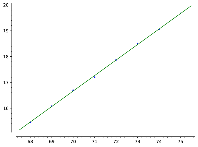
[Zim99]

P. Zimmermann.


Karatsuba square root.


Technical Report RR-3805, Inria, 1999.

		$\displaystyle(-\lfloor R_{0}\rfloor q-r_{0}+a_{0}n_{\circ})m=(-\lfloor R_{0}\rfloor q-(\{R_{0}\}-\beta)q+a_{0}n_{\circ})m$
		$\displaystyle=\left(-\left(\frac{x}{m_{\circ}n_{\circ}}-\frac{x}{m_{\circ}^{2}n_{\circ}}(m-m_{\circ})\right)q+\beta q+a_{0}n_{\circ}\right)m$
		$\displaystyle=\left(-\left(\frac{x}{m_{\circ}n_{\circ}}-\frac{x}{m_{\circ}^{2}n_{\circ}}(m-m_{\circ})\right)+\beta+\left(-\frac{x}{m_{\circ}n_{\circ}^{2}}-\delta\right)n_{\circ}\right)mq$
		$\displaystyle=\left(-\frac{2x}{m_{\circ}n_{\circ}}+\frac{x(m-m_{\circ})}{m_{\circ}^{2}n_{\circ}}+O^{}\left(\frac{1}{2q}\right)+O^{}\left(\frac{1}{2bq}\right)n_{\circ}\right)mq.$

		$\displaystyle\frac{x}{m_{\circ}n_{\circ}}mq\leq\frac{x}{m_{\circ}n_{\circ}}(m_{\circ}+a)\cdot 2b\leq\frac{2bx}{n_{\circ}}+\frac{2abx}{m_{\circ}n_{\circ}}\leq 2x\sqrt[3]{\frac{A}{6x}}+2x\sqrt[3]{\frac{A^{2}}{(6x)^{2}}}$
		$\displaystyle\leq 2x\sqrt[3]{\frac{v}{6x}}+2x\sqrt[3]{\frac{v^{2}}{(6x)^{2}}}\leq 2\sqrt[3]{\frac{c}{6}}\cdot x^{\frac{4}{5}}\left(\frac{\log\log x}{\log x}\right)^{1/5}+2\left(\frac{c}{6}\right)^{\frac{2}{3}}x^{\frac{3}{5}}\left(\frac{\log\log x}{\log x}\right)^{2/5}.$

Summing μ⁡(n)\mu(n): a faster elementary algorithm

Abstract.

1. Introduction

Main Theorem.

1.1. Our approach

1.2. Alternatives

1.3. Notation and algorithmic conventions

1.4. Acknowledgements

2. Preparatory work: identities

3. The case of a large non-free variable

Lemma 3.1.

Proof.

Proposition 3.2.

Proof.

4. The case of a large free variable

4.1. A first try

4.2. Handling the difference between reality and an approximation

Lemma 4.1.

Proof.

Lemma 4.2.

Proof.

Lemma 4.3.

Proof.

Lemma 4.4.

Proof.

Lemma 4.5.

Proof.

Lemma 4.6.

Proof.

5. Parameter choice. Final estimates.

5.1. Bounding the quadratic error term. Choosing aa and bb.

5.2. Choice of vv. Total time and space estimates.

6. Implementation details

7. Numerical results

Appendix A A sketch of an alternative algorithm

Appendix B Pseudocode for algorithms

References

Summing $\mu(n)$ : a faster elementary algorithm

5.1. Bounding the quadratic error term. Choosing $a$ and $b$ .

5.2. Choice of $v$ . Total time and space estimates.