Finite temperature fluctuation-induced order and responses in magnetic topological insulators
Abstract
We derive an effective field theory model for magnetic topological insulators and predict that a magnetic electronic gap persists on the surface for temperatures above the ordering temperature of the bulk. Our analysis also applies to interfaces of heterostructures consisting of a ferromagnetic and a topological insulator. In order to make quantitative predictions for MnBi2Te4 and for EuS-Bi2Se3 heterostructures, we combine the effective field theory method with density functional theory and Monte Carlo simulations. For MnBi2Te4 we predict an upwards Néel temperature shift at the surface up to , while the EuS-Bi2Se3 interface exhibits a smaller relative shift. The effective theory also predicts induced Dzyaloshinskii-Moriya interactions and a topological magnetoelectric effect, both of which feature a finite temperature and chemical potential dependence.
August 11, 2026
Introduction — Since the first experimental observation of the quantum anomalous Hall effect (QAHE) –the appearance of quantized Hall conductance at zero magnetic field– in thin films of the topological insulator (TI) Bi2Se3 doped with magnetic atoms at temperatures below 1 K Liu et al. 2016, magnetic topological materials have been at the scientific forefront both experimentally and theoretically Yokoyama et al. 2010; Garate and Franz 2010; Tserkovnyak and Loss 2012; Nogueira and Eremin 2012; Nogueira and Eremin 2014; Nogueira and Eremin 2013; Tserkovnyak et al. 2015; Rex et al. 2016a; Li et al. 2015; Rex et al. 2016b. The QAHE requires a three-dimensional TI in which long-range magnetic order breaks the time-reversal symmetry, via ferromagnetic Katmis et al. 2016; Wei et al. 2013; Yang et al. 2013; Lee et al. 2016 or antiferromagnetic ordering He et al. 2017. Driven by the major goal to realize quantization of conductance at room temperature, two distinct directions of material-development have triggered much of the recent experimental progress: the successful fabrication of atomically sharp interfaces of ferromagnetic and topological materials, in particular of EuS and Bi2Se3 Wei et al. 2013; Yang et al. 2013; Katmis et al. 2016, and the growth of intrinsically magnetic TIs like MnTe(Bi2Te3)m with Otrokov et al. 2019a; Gong et al. 2019; Zeugner et al. 2019; Vidal et al. 2019a; Otrokov et al. 2019b; Vidal et al. 2019b and MnSb2Te4 Chen et al. 2019a; Wimmer et al. 2020 as highly-ordered single-crystals or their intrinsic heterostructures Hirahara et al. 2017; Hirahara et al. 2020.
Conceptually, a perfectly quantized Hall conductivity of arises at zero temperature when the magnetization couples to the topological Dirac-type TI surface states, opening up a gap there in which then the chemical potential must lie, see Fig. 1. As a bonus, fermionic quantum fluctuations induce a concomitant linear topological magnetoelectric effect (TME), which couples electric fields directly to the magnetization and, vice versa, magnetization dynamics to electrical polarization Qi et al. 2008; Ryu et al. 2012. At zero temperature for outside the gap both Hall conductance and TME fail to be quantized Yokoyama et al. 2010; Nogueira and Eremin 2014; Tutschku et al. 2020, tending to vanish as grows. Nevertheless, this particular situation has the interesting feature, that a Dzyaloshinskii Moriya interaction (DMI) between magnetic degrees of freedom emerges, opening the path towards the formation of various skyrmion-like topological magnetic textures at the surface Nogueira et al. 2018; Tiwari et al. 2019, observed also experimentallyZhang et al. 2018.


The goal to realize the QAHE, TME and possibly even a DMI at room temperature ties into a number of fundamental and practical questions. The first is how in an ideal situation the surface magnetic ordering temperature is affected by coupling to the topological edge states – it has been suggested that this coupling can greatly enhance Katmis et al. 2016; Kim et al. 2017. Subsequently the question is how temperature fluctuations affect the conductance quantization, TME and DMI for the different relevant regimes of . Particularly interesting would be the existence of a temperature regime in which both DMI and TME are sizeable in which case the TME endows external magnetic and electric fields with novel types of access to DMI-induced skyrmions.
Despite the several theoretical and experimental developments in recent years, a number of fundamental questions remain to be answered. For instance, although a remarkable enhancement of at interfaces of certain ferromagnetic insulators (FMIs) have been reported Katmis et al. 2016; Wang et al. 2020, recent works Krieger et al. 2019; Figueroa et al. 2020 question the validity of these findings for the specific case of EuS proximate to either Bi2Se3 or (Bi,Sb)2Te3. Furthermore, a recent experimental work Krieger et al. 2019 indicates that the topological electronic states at the interface do not interact strongly with ferromagnetism for the case of a EuS-Bi2Se3 heterostructure. Additionally, in the family of magnetic TIs MnTe(Bi2Te3)m, different works that do find a surface spectrum gapped below the Néel temperature also observe the persistence of the gap in the paramagnetic phase Otrokov et al. 2019a; Vidal et al. 2019b; Wu et al. 2019, it being unclear whether or not these observations result from the intrinsic magnetism.
Here we develop the finite temperature continuum field theory to address the questions concerning the magnetic phase transitions and dynamics at finite temperature, and apply these results to several experimentally relevant materials systems, using Monte-Carlo simulations (MCS) and density functional theory (DFT) based approaches to obtain quantitative results. Using a minimal model for the coupling of the Dirac fermions to the magnetic Hamiltonian, we show that in a temperature window where bulk magnetism is absent, an out-of-plane surface magnetization can still be nonzero and induce a gap in the Dirac spectrum. As a consequence, the AHE and TME can survive in a certain temperature range above the bulk . However, for the experimentally relevant materials and material combinations (EuS-Bi2Se3, MnBi2Te4), the coupling to the topological surface states enhance the bulk not more than , even under the most favorable conditions. Significant enhancements would require using TIs with a much lower Fermi velocity of the Dirac cone. In addition, at finite we establish the existence of a temperature regime displaying both a substantial fluctuation-induced DMI and TME, even if its Hall conductivity is strongly renormalized, with potentially interesting consequences for skyrmion manipulation and transport.
Saddle-point and induced order — To determine the shift in magnetic ordering temperature due to coupling of the magnetic moments to the fluctuating Dirac fermions we consider the following minimal model Hamiltonian
| (1) |
where the Dirac fermions couple to the magnetization via a magnetic exchange interaction , is the Pauli matrix vector and the unit vector field representing the magnetization direction at . The operator has the property , where . Additionally, an electric potential has been introduced, which includes contributions of an externally applied electric field and an internal long-range Coulomb interaction as well.
The fermionic quantum fluctuations of the Dirac Hamiltonian (1) are accounted for by the imaginary time path integral,
| (2) | ||||
| (3) |
where is a spinor of Grassmann fields obtained from the second-quantized Hamiltonian Negele and Orland 1988. The above partition function defines a free energy functional which provides an additional free energy to the one of the magnetic free energy. As a minimal model leading to the latter, we consider the magnetic Hamiltonian,
| (4) |
where is the exchange energy and is the anisotropy energy density (per unit area). The magnetic partition function is given by the path integral,
| (5) |
where is the Berry phase that arises in the construction of the spin coherent state path integral Sachdev 2011, and is a Lagrange multiplier field enforcing the constraint .
Keeping the magnetic fluctuations classical, we obtain the following effective Hamiltonian after integrating out the Gaussian fluctuations and , along with the fermions,
| (6) | |||||
Variation with respect to leads to the saddle-point equation,
| (7) |
where , is a fermionic Matsubara frequency, and we have defined . Equation (7) is solved together with the saddle-point equation for , which occurs at ,
| (8) |
Setting in Eq. (7) reduces the saddle-point equations to one of a classical ferromagnet with easy-axis anisotropy. In this special case the ordered phase immediately implies and from Eq. (8) it is straightforward to obtain the critical temperature by demanding that , yielding
| (9) |
where a cutoff has been introduced. Note that that the above is consistent with the Mermin-Wagner theorem in the limit .
Our aim is to calculate the shift of this critical temperature when , i.e., accounting for the fermionic quantum fluctuations. After explicitly evaluating the Matsubara sum and integral, Eq. (7) becomes
| (10) |
where the cutoff . The chemical potential is temperature dependent and can be obtained by fixing the particle density. At the critical temperature of the interacting system we demand that and obtain
| (11) |
where . This finally yields the critical temperature shift relative to the situation where fermions are absent,
| (12) |
Since the cutoff is large, it is clear that the argument of the logarithm in Eq. (12) is smaller than unity, and therefore in all cases. From Eqs. (11) and (12) we see that smaller values of favor larger shifts of the critical temperature.
Material specifics — In order to make quantitative predictions for the material systems of interest, we need to determine the values of the coupling parameters and cutoffs appearing in the continuum theory. We base such values on ab-initio and Monte-Carlo calculations, which we find to be consistent with available experimental data.
Based on DFT for a finite slab, for MnBi2Te4 we find the Fermi velocity as eVÅ and the coupling meV, whereas for EuS-Bi2Se3, we consider eVÅ and meV Wei et al. 2013; Eremeev et al. 2015; Zhang et al. 2009. Note, the value of was derived from the gap size in the Dirac dispersion assuming its origin is purely magnetic. In reality higher order effects such as hybridization of the surface fermions with the bulk electronic states of MnBi2Te4 or EuS may also influence the gap such that the actual magnetic gap and correspondingly might be smaller.
For the fermionic cutoff , we consider that the average surface density of a completely filled band is , with the surface unit cell area. Since our model describes two surface bands, we fix such that . Electron-hole symmetry of the model then implies that .
To set the anisotropy and stiffness of the magnetization field, we first build an anisotropic Heisenberg lattice model which we then map to Eq. (4). As the on-site anisotropy depends crucially on the thickness of the FMI layer in the EuS-Bi2Se3 system Katmis et al. 2016, while the Mn layers in MnBi2Te4 are well separated with relatively small out-of-plane exchange couplings Otrokov et al. 2019a; Tan et al. 2020, we consider the magnetic subsystem to be monolayer thick. The corresponding lattice in both cases is a two-dimensional triangular lattice spanned by Mn in MnBi2Te4 and Eu on the EuS surface Katmis et al. 2016. The considered magnetic interactions comprise of nearest neighbor ferromagnetic exchange couplings , and an effective on-site out-of-plane anisotropy . and follow from and taking the continuum limit SI.
For MnBi2Te4, we obtain from DFT calculations meV, and meV, in good agreement with earlier reported values Li et al. 2020. For monolayer EuS, on the other hand, was obtained by extrapolating the data for the nm thick Bi2Se3 layer in the EuS-Bi2Se3 heterostructures in Ref. [Katmis et al. 2016] to the EuS monolayer thickness. We obtain meV. The exchange coupling for the monolayer has been previously estimated to be meV Mauger and Godart 1986. It is interesting that these two material systems cover a broad range of (from in the Mn-based compound to in the EuS-based system).
Last, the spin cutoff was fixed such the critical temperature of the continuum model (without fermions) matches the critical temperature of the corresponding Heisenberg model. To obtain the latter, classical MCS for the lattice model were carried out (see SI SI for details). For the EuS-Bi2Se3 and MnBi2Te4 system, we obtain K and K, respectively. Based on these values, we fix via Eq. (9).
Finally, using Eq. (12), we obtain and for EuS-Bi2Se3 and MnBi2Te4, respectively. Note that the compound having smaller Fermi velocity (MnBi2Te4) shows indeed a larger shift of the critical temperature (recall that in both cases is similar).
Fluctuations around the saddle-point — The question on how the DMI, TME and Hall conductivity evolve with temperature and chemical potential requires considering the effect of magnetic fluctuations in the fermionic determinant resulting from integrating out the fermions. Introducing we can determine the effective action around the saddle-point approximation up to quadratic order in the fluctuations.
The reason for the appearance of the DMI term Nogueira et al. 2018 is that the magnetization fluctuations effectively break the inversion symmetry of our starting Hamiltonian. As a consequence, this yields a DMI contribution to the magnetic free energy,
| (13) |
where,
| (14) |
It is important to emphasize that the DMI term is not introduced in an ad hoc way – it is generated by charge fluctuations coupling to the magnetic moments at the interface. The DMI vanishes at the neutrality point and is nonzero away from it. This creates the possibility of manipulating the DMI by controlling the chemical potential, for instance by gating. If we take the mass to have a mean-field like behavior we find the zero temperature value for the DMI which demonstrates that the DMI kicks in when the Fermi energy surpasses a threshold given by the exchange coupling constant . This feature of the generated DMI can also be seen in Fig. 2 (a) where we show the whole temperature range for different values of the chemical potential with an estimated zero temperature exchange coupling constant of based on our findings for the MnBi2Te4 system. We further see that the lower the temperature gets, the narrower the range for the chemical potential becomes in which there still is a finite DMI. Moreover, we see that the step-function behavior of the generated DMI at zero temperature approximately extends to the whole temperature range as the DMI is only present when the chemical potential exceeds the magnetic gap, meaning it exists only in the metallic regime.


Finally, we determine the fluctuation-induced effective Chern-Simons (CS) action,
| (15) |
where we have defined the covariant three-potential . The electric potential enters in the time component as usual and the magnetization fluctuations act as the vector potential in the spatial components. Note that the ”” applies to the different choices for the vector . The coefficient arising in Eq. (15) leads to the gap in magnetic susceptibility, in a mechanism closely related to the well known topologically massive photons in a Maxwell-Chern-Simons theory Deser et al. 1982. In our case this topological mass is given by,
| (16) |
We recall here that the topological mass arising in the effective free energy is in general not identical to the Hall conductivity — these quantities differ, for instance, in the metallic regime Nogueira and Eremin 2014; Tutschku et al. 2020, something that is more easily seen in the zero temperature limit. Indeed, for the topological mass and Hall conductivity are given by Nogueira and Eremin 2014 and , respectively. These zero temperature expressions involving the Heaviside step function are identical only when . In fact, vanishes in the metallic regime while is nonzero. This occurs because the Hall conductivity is calculated from the Kubo formula where one first takes the limit and then , while in case of the topological mass these limits are taken simultaneously. The CS action (15) contains the TME contribution to the free energy,
| (17) |
To compare its features to the ones of the DMI we also illustrate its dependency on temperature and chemical potential in Fig. 2 (b). Once more it shows that at zero temperature we have a step function behavior which also approximately extends to finite temperatures. Consequently, the topological mass only exists when the chemical potential lies inside the magnetic gap and is nearly quantized in the bordering regions resulting into plateaus. In comparison to the generated DMI we can see in Fig. 3 that there is a very narrow region where both functions overlap. As a result, the desired simultaneous occurrence of the DMI and the CS action requires fine tuning.

However, upon closer inspection, a different connection between the two terms appears. It turns out that the temperature functions inside both terms complement each other almost perfectly in a temperature and chemical potential plot, as also can be seen for exemplary temperatures in Fig. 3. The two functions are adding up to one creating a plateau that even traverses the chasm that both functions showed individually in the vicinity where the chemical potential crossed the magnetic gap. This means that at the time one of the terms diminishes, the respective other term grows in size equal to the loss of the other, creating a direct correspondence between them. We point out that besides the DMI and CS terms, other interesting terms appear in the effective action, as is shown in explicitly in the SI SI.
Conclusion — We have considered a minimal model for magnetic topological insulators that capture a wealth of interesting properties of the surface of materials like MnTe(Bi2Te3)m with Otrokov et al. 2019a; Zeugner et al. 2019; Otrokov et al. 2019b; Vidal et al. 2019b and MnSb2Te4 Chen et al. 2019a; Wimmer et al. 2020, and also at interfaces of heterostructures EuS-Bi2Se3 Wei et al. 2013; Yang et al. 2013; Katmis et al. 2016. An important main result of our analysis is the prediction of the survival of the electronic gap on the surface/interface for temperatures above the bulk ordering temperature. In order to provide quantitative results to be compared with experiment, we have combined the effective field theory analysis with DFT and MCS results applied specifically to MnBi2Te4 and the bilayer system EuS-Bi2Se3. We also predict that temperature dependent DMI and TME terms are induced by fluctuations. The latter may give rise to new magnetic phenomena at the surface of magnetic TIs, including the interesting possibility of manipulating skyrmions by external or internal electrical fields.
Acknowledgements.
JvdB acknowledges support by the DFG through the Würzburg-Dresden Cluster of Excellence on Complexity and Topology in Quantum Matter – ct.qmat (EXC 2147, project-id 39085490) and through SFB 1143 (project-id 247310070). JIF would like to thank the support of the Alexander von Humboldt Foundation. I.E. would like to thank the DFG Priority Program SPP 1666, “Topological Insulators,” under Grant No.ER 463/9. The authors thank Ulrike Nitzsche for technical assistance.References
- Liu et al. (2016) Chao-Xing Liu, Shou-Cheng Zhang, and Xiao-Liang Qi, “The quantum anomalous hall effect: Theory and experiment,” Annual Review of Condensed Matter Physics 7, 301–321 (2016).
- Yokoyama et al. (2010) Takehito Yokoyama, Jiadong Zang, and Naoto Nagaosa, “Theoretical study of the dynamics of magnetization on the topological surface,” Phys. Rev. B 81, 241410 (2010).
- Garate and Franz (2010) Ion Garate and M. Franz, “Inverse Spin-Galvanic Effect in the Interface between a Topological Insulator and a Ferromagnet,” Phys. Rev. Lett. 104, 146802 (2010).
- Tserkovnyak and Loss (2012) Yaroslav Tserkovnyak and Daniel Loss, “Thin-Film Magnetization Dynamics on the Surface of a Topological Insulator,” Phys. Rev. Lett. 108, 187201 (2012).
- Nogueira and Eremin (2012) Flavio S. Nogueira and Ilya Eremin, “Fluctuation-Induced Magnetization Dynamics and Criticality at the Interface of a Topological Insulator with a Magnetically Ordered Layer,” Phys. Rev. Lett. 109, 237203 (2012).
- Nogueira and Eremin (2014) Flavio S. Nogueira and Ilya Eremin, “Thermal screening at finite chemical potential on a topological surface and its interplay with proximity-induced ferromagnetism,” Phys. Rev. B 90, 014431 (2014).
- Nogueira and Eremin (2013) Flavio S. Nogueira and Ilya Eremin, “Semimetal-insulator transition on the surface of a topological insulator with in-plane magnetization,” Phys. Rev. B 88, 085126 (2013).
- Tserkovnyak et al. (2015) Yaroslav Tserkovnyak, D. A. Pesin, and Daniel Loss, “Spin and orbital magnetic response on the surface of a topological insulator,” Phys. Rev. B 91, 041121 (2015).
- Rex et al. (2016a) Stefan Rex, Flavio S. Nogueira, and Asle Sudbø, “Nonlocal topological magnetoelectric effect by Coulomb interaction at a topological insulator-ferromagnet interface,” Phys. Rev. B 93, 014404 (2016a).
- Li et al. (2015) Mingda Li, Wenping Cui, Jin Yu, Zuyang Dai, Zhe Wang, Ferhat Katmis, Wanlin Guo, and Jagadeesh Moodera, “Magnetic proximity effect and interlayer exchange coupling of ferromagnetic/topological insulator/ferromagnetic trilayer,” Phys. Rev. B 91, 014427 (2015).
- Rex et al. (2016b) Stefan Rex, Flavio S. Nogueira, and Asle Sudbø, “Topological magnetic dipolar interaction and nonlocal electric magnetization control in topological insulator heterostructures,” Phys. Rev. B 94, 020404 (2016b).
- Katmis et al. (2016) Ferhat Katmis, Valeria Lauter, Flavio S. Nogueira, Badih A. Assaf, Michelle E. Jamer, Peng Wei, Biswarup Satpati, John W. Freeland, Ilya Eremin, Don Heiman, Pablo Jarillo-Herrero, and Jagadeesh S. Moodera, “A high-temperature ferromagnetic topological insulating phase by proximity coupling,” Nature 533, 513–516 (2016).
- Wei et al. (2013) Peng Wei, Ferhat Katmis, Badih A. Assaf, Hadar Steinberg, Pablo Jarillo-Herrero, Donald Heiman, and Jagadeesh S. Moodera, “Exchange-Coupling-Induced Symmetry Breaking in Topological Insulators,” Phys. Rev. Lett. 110, 186807 (2013).
- Yang et al. (2013) Qi I. Yang, Merav Dolev, Li Zhang, Jinfeng Zhao, Alexander D. Fried, Elizabeth Schemm, Min Liu, Alexander Palevski, Ann F. Marshall, Subhash H. Risbud, and Aharon Kapitulnik, “Emerging weak localization effects on a topological insulator–insulating ferromagnet (Bi2Se3-EuS) interface,” Phys. Rev. B 88, 081407 (2013).
- Lee et al. (2016) Changmin Lee, Ferhat Katmis, Pablo Jarillo-Herrero, Jagadeesh S. Moodera, and Nuh Gedik, “Direct measurement of proximity-induced magnetism at the interface between a topological insulator and a ferromagnet,” Nature Communications 7, 12014 (2016).
- He et al. (2017) Qing Lin He, Xufeng Kou, Alexander J. Grutter, Gen Yin, Lei Pan, Xiaoyu Che, Yuxiang Liu, Tianxiao Nie, Bin Zhang, Steven M. Disseler, Brian J. Kirby, William Ratcliff II, Qiming Shao, Koichi Murata, Xiaodan Zhu, Guoqiang Yu, Yabin Fan, Mohammad Montazeri, Xiaodong Han, Julie A. Borchers, and Kang L. Wang, “Tailoring exchange couplings in magnetic topological-insulator/antiferromagnet heterostructures,” Nature Materials 16, 94–100 (2017).
- Otrokov et al. (2019a) M. M. Otrokov, I. I. Klimovskikh, H. Bentmann, D. Estyunin, A. Zeugner, Z. S. Aliev, S. Gaß, A. U. B. Wolter, A. V. Koroleva, A. M. Shikin, M. Blanco-Rey, M. Hoffmann, I. P. Rusinov, A. Yu. Vyazovskaya, S. V. Eremeev, Yu. M. Koroteev, V. M. Kuznetsov, F. Freyse, J. Sánchez-Barriga, I. R. Amiraslanov, M. B. Babanly, N. T. Mamedov, N. A. Abdullayev, V. N. Zverev, A. Alfonsov, V. Kataev, B. Büchner, E. F. Schwier, S. Kumar, A. Kimura, L. Petaccia, G. Di Santo, R. C. Vidal, S. Schatz, K. Kißner, M. Ünzelmann, C. H. Min, Simon Moser, T. R. F. Peixoto, F. Reinert, A. Ernst, P. M. Echenique, A. Isaeva, and E. V. Chulkov, “Prediction and observation of an antiferromagnetic topological insulator,” Nature 576, 416–422 (2019a).
- Gong et al. (2019) Yan Gong, Jingwen Guo, Jiaheng Li, Kejing Zhu, Menghan Liao, Xiaozhi Liu, Qinghua Zhang, Lin Gu, Lin Tang, Xiao Feng, Ding Zhang, Wei Li, Canli Song, Lili Wang, Pu Yu, Xi Chen, Yayu Wang, Hong Yao, Wenhui Duan, Yong Xu, Shou-Cheng Zhang, Xucun Ma, Qi-Kun Xue, and Ke He, “Experimental Realization of an Intrinsic Magnetic Topological Insulator,” Chinese Physics Letters 36, 076801 (2019).
- Zeugner et al. (2019) Alexander Zeugner, Frederik Nietschke, Anja U. B. Wolter, Sebastian Gaß, Raphael C. Vidal, Thiago R. F. Peixoto, Darius Pohl, Christine Damm, Axel Lubk, Richard Hentrich, Simon K. Moser, Celso Fornari, Chul Hee Min, Sonja Schatz, Katharina Kißner, Maximilian Ünzelmann, Martin Kaiser, Francesco Scaravaggi, Bernd Rellinghaus, Kornelius Nielsch, Christian Hess, Bernd Büchner, Friedrich Reinert, Hendrik Bentmann, Oliver Oeckler, Thomas Doert, Michael Ruck, and Anna Isaeva, “Chemical Aspects of the Candidate Antiferromagnetic Topological Insulator MnBi2Te4,” Chemistry of Materials 31, 2795–2806 (2019).
- Vidal et al. (2019a) R. C. Vidal, H. Bentmann, T. R. F. Peixoto, A. Zeugner, S. Moser, C.-H. Min, S. Schatz, K. Kißner, M. Ünzelmann, C. I. Fornari, H. B. Vasili, M. Valvidares, K. Sakamoto, D. Mondal, J. Fujii, I. Vobornik, S. Jung, C. Cacho, T. K. Kim, R. J. Koch, C. Jozwiak, A. Bostwick, J. D. Denlinger, E. Rotenberg, J. Buck, M. Hoesch, F. Diekmann, S. Rohlf, M. Kalläne, K. Rossnagel, M. M. Otrokov, E. V. Chulkov, M. Ruck, A. Isaeva, and F. Reinert, “Surface states and Rashba-type spin polarization in antiferromagnetic MnBi2Te4(0001),” Phys. Rev. B 100, 121104 (2019a).
- Otrokov et al. (2019b) M. M. Otrokov, I. P. Rusinov, M. Blanco-Rey, M. Hoffmann, A. Yu. Vyazovskaya, S. V. Eremeev, A. Ernst, P. M. Echenique, A. Arnau, and E. V. Chulkov, “Unique Thickness-Dependent Properties of the van der Waals Interlayer Antiferromagnet MnBi2Te4 Films,” Phys. Rev. Lett. 122, 107202 (2019b).
- Vidal et al. (2019b) Raphael C. Vidal, Alexander Zeugner, Jorge I. Facio, Rajyavardhan Ray, M. Hossein Haghighi, Anja U. B. Wolter, Laura T. Corredor Bohorquez, Federico Caglieris, Simon Moser, Tim Figgemeier, Thiago R. F. Peixoto, Hari Babu Vasili, Manuel Valvidares, Sungwon Jung, Cephise Cacho, Alexey Alfonsov, Kavita Mehlawat, Vladislav Kataev, Christian Hess, Manuel Richter, Bernd Büchner, Jeroen van den Brink, Michael Ruck, Friedrich Reinert, Hendrik Bentmann, and Anna Isaeva, “Topological Electronic Structure and Intrinsic Magnetization in : A Derivative with a Periodic Mn Sublattice,” Phys. Rev. X 9, 041065 (2019b).
- Chen et al. (2019a) Bo Chen, Fucong Fei, Dongqin Zhang, Bo Zhang, Wanling Liu, Shuai Zhang, Pengdong Wang, Boyuan Wei, Yong Zhang, Zewen Zuo, et al., “Intrinsic magnetic topological insulator phases in the Sb doped MnBi2Te4 bulks and thin flakes,” Nature Communications 10, 1–8 (2019a).
- Wimmer et al. (2020) S. Wimmer, J. Sánchez-Barriga, P. Küppers, A. Ney, E. Schierle, F. Freyse, O. Caha, J. Michalicka, M. Liebmann, D. Primetzhofer, M. Hoffmann, A. Ernst, M. M. Otrokov, G. Bihlmayer, E. Weschke, B. Lake, E. V. Chulkov, M. Morgenstern, G. Bauer, G. Springholz, and O. Rader, “Ferromagnetic MnSb2Te4: A topological insulator with magnetic gap closing at high Curie temperatures of 45-50 K,” (2020), arXiv:2011.07052 [cond-mat.mtrl-sci] .
- Hirahara et al. (2017) Toru Hirahara, Sergey V. Eremeev, Tetsuroh Shirasawa, Yuma Okuyama, Takayuki Kubo, Ryosuke Nakanishi, Ryota Akiyama, Akari Takayama, Tetsuya Hajiri, Shin ichiro Ideta, Masaharu Matsunami, Kazuki Sumida, Koji Miyamoto, Yasumasa Takagi, Kiyohisa Tanaka, Taichi Okuda, Toshihiko Yokoyama, Shin ichi Kimura, Shuji Hasegawa, and Evgueni V. Chulkov, “Large-Gap Magnetic Topological Heterostructure Formed by Subsurface Incorporation of a Ferromagnetic Layer,” Nano Letters 17, 3493–3500 (2017).
- Hirahara et al. (2020) T. Hirahara, M. M. Otrokov, T. T. Sasaki, K. Sumida, Y. Tomohiro, S. Kusaka, Y. Okuyama, S. Ichinokura, M. Kobayashi, Y. Takeda, K. Amemiya, T. Shirasawa, S. Ideta, K. Miyamoto, K. Tanaka, S. Kuroda, T. Okuda, K. Hono, S. V. Eremeev, and E. V. Chulkov, “Fabrication of a novel magnetic topological heterostructure and temperature evolution of its massive Dirac cone,” Nature Communications 11, 4821 (2020).
- Qi et al. (2008) Xiao-Liang Qi, Taylor L. Hughes, and Shou-Cheng Zhang, “Topological field theory of time-reversal invariant insulators,” Phys. Rev. B 78, 195424 (2008).
- Ryu et al. (2012) Shinsei Ryu, Joel E. Moore, and Andreas W. W. Ludwig, “Electromagnetic and gravitational responses and anomalies in topological insulators and superconductors,” Phys. Rev. B 85, 045104 (2012).
- Tutschku et al. (2020) Christian Tutschku, Flavio S. Nogueira, Christian Northe, Jeroen van den Brink, and E. M. Hankiewicz, “Temperature and chemical potential dependence of the parity anomaly in quantum anomalous hall insulators,” Phys. Rev. B 102, 205407 (2020).
- Nogueira et al. (2018) Flavio S. Nogueira, Ilya Eremin, Ferhat Katmis, Jagadeesh S. Moodera, Jeroen van den Brink, and Volodymyr P. Kravchuk, “Fluctuation-induced Néel and Bloch skyrmions at topological insulator surfaces,” Phys. Rev. B 98, 060401 (2018).
- Tiwari et al. (2019) Kunal L. Tiwari, J. Lavoie, T. Pereg-Barnea, and W. A. Coish, “Tunable skyrmion-skyrmion binding on the surface of a topological insulator,” Phys. Rev. B 100, 125414 (2019).
- Zhang et al. (2018) Shilei Zhang, Florian Kronast, Gerrit van der Laan, and Thorsten Hesjedal, “Real-Space Observation of Skyrmionium in a Ferromagnet-Magnetic Topological Insulator Heterostructure,” Nano Letters 18, 1057–1063 (2018).
- Kim et al. (2017) Jeongwoo Kim, Kyoung-Whan Kim, Hui Wang, Jairo Sinova, and Ruqian Wu, “Understanding the Giant Enhancement of Exchange Interaction in Bi2Se3–EuS Heterostructures,” Phys. Rev. Lett. 119, 027201 (2017).
- Wang et al. (2020) Haiyu Wang, Yingjie Liu, Peichen Wu, Wenjie Hou, Yuhao Jiang, Xiaohui Li, Chandan Pandey, Dongdong Chen, Qing Yang, Hangtian Wang, Dahai Wei, Na Lei, Wang Kang, Lianggong Wen, Tianxiao Nie, Weisheng Zhao, and Kang L. Wang, “Above Room-Temperature Ferromagnetism in Wafer-Scale Two-Dimensional van der Waals Fe3GeTe2 Tailored by a Topological Insulator,” ACS Nano 14, 10045–10053 (2020).
- Krieger et al. (2019) J. A. Krieger, Y. Ou, M. Caputo, A. Chikina, M. Döbeli, M.-A. Husanu, I. Keren, T. Prokscha, A. Suter, Cui-Zu Chang, J. S. Moodera, V. N. Strocov, and Z. Salman, “Do topology and ferromagnetism cooperate at the EuS/Bi2Se3 interface?” Phys. Rev. B 99, 064423 (2019).
- Figueroa et al. (2020) A. I. Figueroa, F. Bonell, M. G. Cuxart, M. Valvidares, P. Gargiani, G. van der Laan, A. Mugarza, and S. O. Valenzuela, “Absence of Magnetic Proximity Effect at the Interface of Bi2Se3 and (Bi, Sb)2Te3 with EuS,” Phys. Rev. Lett. 125, 226801 (2020).
- Wu et al. (2019) Jiazhen Wu, Fucai Liu, Masato Sasase, Koichiro Ienaga, Yukiko Obata, Ryu Yukawa, Koji Horiba, Hiroshi Kumigashira, Satoshi Okuma, Takeshi Inoshita, et al., “Natural van der Waals heterostructural single crystals with both magnetic and topological properties,” Science advances 5, eaax9989 (2019).
- Negele and Orland (1988) John W. Negele and Henri Orland, Quantum Many-Particle Systems (Addison-Wesley, Reading, MA, 1988).
- Sachdev (2011) S. Sachdev, Quantum Phase Transitions, 2nd ed. (Cambridge University Press, 2011).
- Eremeev et al. (2015) S.V. Eremeev, V.N. Men’shov, V.V. Tugushev, and E.V. Chulkov, “Interface induced states at the boundary between a 3D topological insulator and a ferromagnetic insulator EuS,” Journal of Magnetism and Magnetic Materials 383, 30–33 (2015).
- Zhang et al. (2009) Haijun Zhang, Chao-Xing Liu, Xiao-Liang Qi, Xi Dai, Zhong Fang, and Shou-Cheng Zhang, “Topological insulators in Bi2Se3, Bi2Te3 and Sb2Te3 with a single Dirac cone on the surface,” Nature Physics 5, 438–442 (2009).
- Tan et al. (2020) Aoyu Tan, Valentin Labracherie, Narayan Kunchur, Anja U. B. Wolter, Joaquin Cornejo, Joseph Dufouleur, Bernd Büchner, Anna Isaeva, and Romain Giraud, “Metamagnetism of Weakly Coupled Antiferromagnetic Topological Insulators,” Phys. Rev. Lett. 124, 197201 (2020).
- (43) “See Supplemental Information xxxx, where we cite the references Perdew et al. 1996; Koepernik and Eschrig 1999; fpl; Vidal et al. 2020; Chen et al. 2019b; Vicente et al. 1999; Wachter 1972; Story et al. 2000; Ghaemi et al. 2001,” .
- Li et al. (2020) Bing Li, J.-Q. Yan, D. M. Pajerowski, Elijah Gordon, A.-M. Nedić, Y. Sizyuk, Liqin Ke, P. P. Orth, D. Vaknin, and R. J. McQueeney, “Competing Magnetic Interactions in the Antiferromagnetic Topological Insulator ,” Phys. Rev. Lett. 124, 167204 (2020).
- Mauger and Godart (1986) A. Mauger and C. Godart, “The magnetic, optical, and transport properties of representatives of a class of magnetic semiconductors: The europium chalcogenides,” Physics Reports 141, 51–176 (1986).
- Deser et al. (1982) S. Deser, R. Jackiw, and S. Templeton, “Three-Dimensional Massive Gauge Theories,” Phys. Rev. Lett. 48, 975–978 (1982).
- Perdew et al. (1996) John P. Perdew, Kieron Burke, and Matthias Ernzerhof, “Generalized Gradient Approximation Made Simple,” Phys. Rev. Lett. 77, 3865–3868 (1996).
- Koepernik and Eschrig (1999) Klaus Koepernik and Helmut Eschrig, “Full-potential nonorthogonal local-orbital minimum-basis band-structure scheme,” Phys. Rev. B 59, 1743–1757 (1999).
- (49) https://www.fplo.de.
- Vidal et al. (2020) R. C. Vidal, H. Bentmann, J. I. Facio, P. Kagerer, C. I. Fornari, T. R. F. Peixoto, T. Figgemeier, S. Jung, C. Cacho, B. Büchner, J. van den Brink, E. F. Schwier, K. Shimada, M. Richter, A. Isaeva, and F. Reinert, “Orbital Complexity in Intrinsic Magnetic Topological Insulators MnBi4Te7 and MnBi6Te10,” (2020), arXiv:2007.07637 [cond-mat.str-el] .
- Chen et al. (2019b) Y. J. Chen, L. X. Xu, J. H. Li, Y. W. Li, H. Y. Wang, C. F. Zhang, H. Li, Y. Wu, A. J. Liang, C. Chen, S. W. Jung, C. Cacho, Y. H. Mao, S. Liu, M. X. Wang, Y. F. Guo, Y. Xu, Z. K. Liu, L. X. Yang, and Y. L. Chen, “Topological Electronic Structure and Its Temperature Evolution in Antiferromagnetic Topological Insulator ,” Phys. Rev. X 9, 041040 (2019b).
- Vicente et al. (1999) C. Pérez Vicente, J. L. Tirado, K. Adouby, J. C. Jumas, A. Abba Touré, and G. Kra, “X-ray Diffraction and 119Sn Mössbauer Spectroscopy Study of a New Phase in the Bi2Se3-SnSe System: SnBi4Se7,” Inorganic Chemistry 38, 2131–2135 (1999).
- Wachter (1972) P. Wachter, “The optical electrical and magnetic properties of the europium chalcogenides and the rare earth pnictides,” C R C Critical Reviews in Solid State Sciences 3, 189–241 (1972).
- Story et al. (2000) T. Story, C. H. W. Swüste, H.J.M. Swagten, W. J. M. de Jonge, A. Stachow-Wójcik, A. Twardowski, M. Arciszewska, W. Dobrowolski, R. R. Gałazka, and A. Yu. Sipatov, “Magnetic Anisotropy in Eus-PbS Multilayers,” Acta Physica Polonica A 97, 435–438 (2000).
- Ghaemi et al. (2001) M. Ghaemi, G. A. Parsafar, and M. Ashrafizaadeh, “Calculation of the Critical Temperature for 2- and 3-Dimensional Ising Models and for 2-Dimensional Potts Models Using the Transfer Matrix Method,” The Journal of Physical Chemistry B 105, 10355–10359 (2001).
Appendix A Supplemental Materials
Appendix B Saddle-point and induced order
The starting point of our field theory is the partition function from the main text, consisting of two parts, namely the magnetic and fermionic contributions. We calculate this partition function in the imaginary time path integral formalism integrating out the fermionic and bosonic fields respectively. Keeping the magnetic fluctuations classical, we look at the magnetic partition function and define a corresponding magnetic action
| (18) |
where the magnetic action is given by
| (19) |
Here we already split up the different components of the magnetization into in-plane and out-of-plane components, where the sum over denotes the and components, such that in the next step we can perform the path integration over the Gaussian fluctuations and yielding the effective action
| (20) |
Doing the same for the fermionic partition function, just by integration over the fermionic fields we get
| (21) |
To note is the additional minus sign in front, resulting from the integration over fermionic fields instead of bosonic ones. Furthermore, the two so defined functional traces differ from each other, which will soon become apparent. Combining the two individual contributions we get the total effective action
| (22) | |||||
which implies the effective Hamiltonian given in the main text.
In the next step we apply the saddle-point approximation to the remaining fields to be integrated over
| (23) |
leading to the saddle point effective action
| (24) | |||||
To keep the notation short we redefine and by dropping the tilde over both quantities. With this we calculate the functional traces
| (25) |
where
| (26) |
which upon reinsertion gives
| (27) |
Similarly, the functional trace from the integration over the fermionic fields is given by
| (28) |
where
| (29) |
with the fermionic Matsubara frequencies . Therefore the functional trace yields
| (30) |
where the sum runs over and we defined with the mass . Using this we can now formulate the saddle point equations by variation of the effective action with respect to
| (31) |
and with respect to
| (32) |
Setting in Eq. (31) reduces the saddle-point equations to one of a classical ferromagnet with easy-axis anisotropy. In this special case the ordered phase immediately implies and from Eq. (32) it is straightforward to obtain the critical temperature by demanding that , yielding
| (33) |
where a cutoff has been introduced. Our aim is to calculate the shift of this critical temperature when , i.e. accounting to the fermionic quantum fluctuations. After explicitly evaluating the Matsubara sum and integral, Eq. (31) becomes,
| (34) |
where we have assumed that the cutoff . The chemical potential is temperature dependent and can be obtained by fixing the particle density. At the critical temperature , we demand that and obtain
| (35) |
where . Analogously to Eq. (33) we then get
| (36) |
This finally yields the critical temperature shift relative to the situation where fermions are absent,
| (37) |
Since the cutoff is large, it is clear that the argument of the logarithm in Eq. (37) is smaller than unity, and therefore .
Appendix C Surface particle density and fermionic cutoff
The fermionic cutoff can be determined from the two dimensional surface particle density given by
| (38) |
where in our case the energies are resulting from the Dirac Hamiltonian. By insertion of these energies into Eq. (38) the surface particle density becomes
| (39) |
where is given by
| (40) |
with the notation for the polylogarithm.
We now consider that the average surface density of a completely filled band is , with the surface unit cell area . Since our model describes two surface bands, we fix such that . At the Integral vanishes, giving an expression for the fermionic cutoff .
Appendix D Mapping between lattice and continuum spin models
We start with an anisotropic Heisenberg model on a two-dimensional triangular lattice:
| (41) |
where, is the nearest neighbor ferromagnetic Heisenberg exchange coupling and is the on-site magnetic anisotropy. Introducing and as the distance vector between lattice site and the Hamiltonian becomes
| (42) |
The (isotropic) Heisenberg exchange term is given by the first part:
| (43) |
Here, the scalar product can be written as
| (44) |
where, in the last step, we retain terms up to in . Therefore, the exchange term becomes
| (45) |
After carrying out the sum over for our triangular lattice, we have
| (46) |
To obtain the continuum limit, we make the substitution
| (47) |
eventually leading to
| (48) |
for the Hamiltonian, where is the unit cell area of the plane perpendicular to the anisotropy direction. Equating the above with the continuum limit Hamiltonian in Eq. (4) of the main text, we obtain the relation between the exchange coupling and the on-site magnetic anisotropy in the two models
| (49) | ||||
| (50) |
Appendix E Material specific parameters and computational details
E.0.1 MnBi2Te4
Density functional theory (DFT) calculations were performed based on experimental bulk crystal structure of MnBi2Te4 using the GGA+ method with the Perdew-Burke-Ernzerhof (PBE) approach Perdew et al. 1996 as implemented in the FPLO code version 18.00-52 Koepernik and Eschrig 1999; fpl. We used the atomic limit double counting correction and tetrahedron method for -space integrations. For the slab calculation, we used a mesh of subdivisions in the Brillouin zone (and for the density of states calculation), while for the bulk calculations we used (rhombohedral setup).
To estimate the magnetic anisotropy , we did calculations for the bulk system, ferromagnetic configuration, with quantization axis along [001] or [100]. The results are sensitive to the values of and used to treat electronic correlations in the Mn- shell. Varying between 1 and 5.34 eV, we find that the magnetic anisotropy energy varies between 0.46 meV and 0.27 meV per Mn or, accordingly, the on-site anisotropy for the Heisenberg model with , , between meV and meV. Similarly, based on additional calculations where the Mn are ordered ferromagnetically between layers and antiferromagnetically within layers, we estimate the intralayer exchange coupling . In the same range of as above, we find to vary between 0.18 meV and 0.5 meV. The trends are similar to those reported in Ref. Li et al. 2020. For the Monte Carlo simulations, we used the values obtained with , which yield the ratio , in very good agreement with Ref. Li et al. 2020.
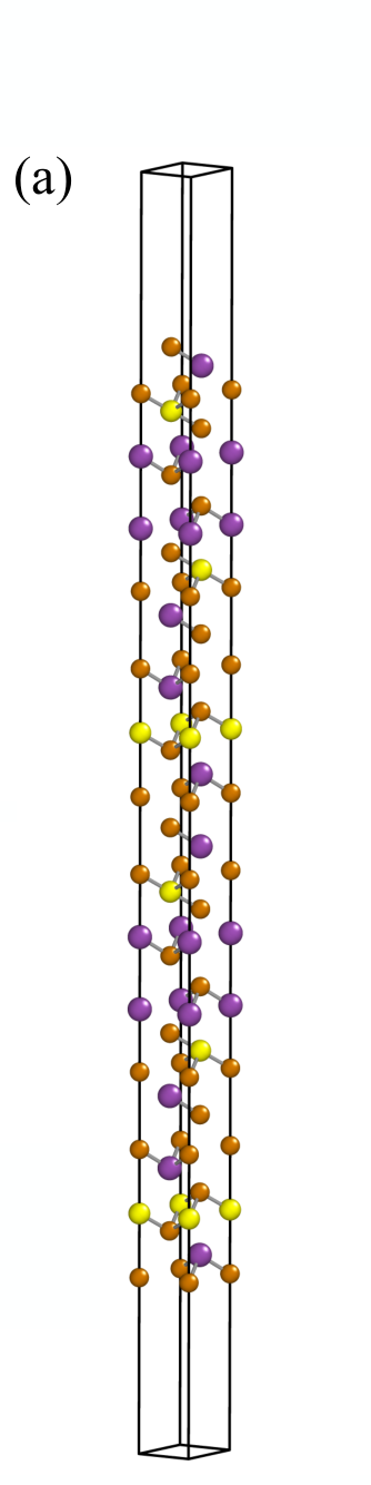
To estimate the Fermi velocity of the surface state and the surface gap, we performed DFT calculations for a slab structure consisting of six MnBi2Te4 unit cells with a vacuum of 30 Bohr radii [Fig. 4(a)]. Following Ref. Otrokov et al. 2019a; Vidal et al. 2020, we fix eV and . The two main surface bands present a gap 100 meV, as shown in Fig. 4(b), in good agreement with the value of 88 meV found in Otrokov et al. 2019a. The Fermi velocity found for the upper part of the Dirac cone is approximately eVÅ in good agreement with the experimental results in Ref. Chen et al. 2019b and DFT results in Ref. Otrokov et al. 2019a.
Lastly, samples of MnBi2Te4 tend to be self-doped, meaning that different kind of defects place the chemical potential outside the gap. In particular, the samples tend to be electron-doped. To estimate the value of , we consider the estimation of carriers of cm3 provided in Ref. Otrokov et al. 2019a. Based on this value and on our slab calculation we estimate meV above the bottom of the conduction band.
Notice that the value of meV with respect to the bottom of the conduction band corresponds to meV with respect to our zero of energies, as we have to add half the size of the gap.
E.0.2 EuS-Bi2Se3 heterostructures
In EuS-Bi2Se3 heterostructures, the interface is typically formed by the surface of the cubic bulk-EuS structure such that the lattice mismatch with the topological Bi2Se3 film is minimal Vicente et al. 1999. For this surface, the interfacial layer of Eu atoms span a triangular lattice. The effective lattice constant of this lattice is , using Wachter 1972.
The Fermi velocity was obtained from Zhang et al. 2009 to approximately be for bulk . Furthermore, the exchange coupling constant was estimated in alignment with the magnetic gap reported in Wei et al. 2013; Eremeev et al. 2015 to have a value of meV.
Regarding magnetism in the EuS-Bi2Se3, the value of meV has been reported earlier Mauger and Godart 1986. The value of the on-site magnetic anisotropy was obtained from the EuS layer thickness dependence of the magnetic anisotropy Katmis et al. 2016. We considered the structure with the largest Bi2Se3 layer thickness of 20 nm. Note that these values are available in the continuum limit and were converted to the lattice equivalent values using Eq. (50). The resulting data was modeled with Story et al. 2000:
| (51) |
where and , respectively denote the bulk and surface magnetic anisotropy contributions and is the thickness of the EuS layer. For the EuS monolayer along the -direction, with a thickness of , we obtain meV, leading to .
E.0.3 Monte-Carlo calculations of
Classical Monte-Carlo simulations (MCS) with the Metropolis algorithm were carried out for spins on a two-dimensional triangular lattice with sites. We consider the spin Hamiltonian of Eq. (41). defines the energy scale leaving the ratio as the only free parameter. For each , we started from a high-temperature paramagnetic state, characterized by a random spin configuration, and decreased the temperature in steps of 0.02. At each temperature, the system was allowed to equilibrate over steps and the physical quantities were obtained by averaging over the next steps. For , the equilibration was typically reached in , however, to treat the entire range of on same footing, we generously consider and steps. The critical temperature, , was obtained from peak(s) in the specific heat, which agrees with corresponding values obtained from the magnetization data vs. .
To address the materials of interest in this study, we used for MnBi2Te4 and for the EuS-Bi2Se3 heterostructure as discussed earlier. Figure 5 (a) shows the corresponding specific heat data. From the well-defined peaks, we obtain and , for the MnBi2Te4 and EuS-Bi2Se3 monolayers, respectively. Considering for MnBi2Te4, we obtain K, while for the EuS-Bi2Se3 heterostructure, yields K.
For completeness, we also carried out MCS over a wide range of . This allows us to study the evolution of as a function of and to analyze how close or far are the systems of interest from the Ising limit . With increasing , the accessible phase space becomes considerably smaller. Consequently, the equilibration is slower. Therefore, for , MCS were carried out with a total of update steps, out of which the first steps correspond to and were discarded during the averaging and evaluation of the physical properties such as specific heat. Figure 5 (b) shows the evolution of with . The Ising limit, which corresponds to Ghaemi et al. 2001, is approximately reached for .
E.1 Fluctuations away from the saddle point
Starting with the same model Hamiltonian but now also accounting for fluctuations around the previously analyzed saddle-point we assume the magnetization to have the form and also for there to be an electric potential , which is of either external or internal origin. The dimensionless euclidean action of our partition function is then given by
| (52) |
where we defined the bosonic Matsubara frequencies and
| (53) | ||||
| (54) |
Performing the path integration over the fermionic fields in the saddle-point approximation yields the fermionic effective action up to second order
| (55) |
where the Greek indices label the spin components resulting from the trace over the Pauli matrices and where we defined
| (56) |
By insertion of the definition of into Eq. (55) one can now split up the different parts of the action according to their magnetoelectric nature, yielding an electric, magnetic and magnetoelectric contribution.
To arrive at the DMI and CS terms we then trace out the spin components, and calculate the integral over and the sum over fermionic Matsubara frequencies in a derivative expansion, that means a long wavelength and low frequency expansion in terms of the wavevector and bosonic Matsubara frequencies . This step is straightforward but very lengthy and shall be omitted here.
Afterwards one transforms back to Euclidean spacetime using the remaining Matsubara sum and momentum integral over and to find the result for the DMI and CS terms presented in the main text, among other contributions.