Online Streaming End-to-End Neural Diarization
Handling Overlapping Speech and Flexible Numbers of Speakers
Abstract
We propose a streaming diarization method based on an end-to-end neural diarization (EEND) model, which handles flexible numbers of speakers and overlapping speech. In our previous study, the speaker-tracing buffer (STB) mechanism was proposed to achieve a chunk-wise streaming diarization using a pre-trained EEND model. STB traces the speaker information in previous chunks to map the speakers in a new chunk. However, it only worked with two-speaker recordings. In this paper, we propose an extended STB for flexible numbers of speakers, FLEX-STB. The proposed method uses a zero-padding followed by speaker-tracing, which alleviates the difference in the number of speakers between a buffer and a current chunk. We also examine buffer update strategies to select important frames for tracing multiple speakers. Experiments on CALLHOME and DIHARD II datasets show that the proposed method achieves comparable performance to the offline EEND method with 1-second latency. The results also show that our proposed method outperforms recently proposed chunk-wise diarization methods based on EEND (BW-EDA-EEND).
2 Language Technologies Institute, Carnegie Mellon University, USA
3 Center for Language and Speech Processing, Johns Hopkins University, USA††email: yawen.xue.wn@hitachi.com
Index Terms: online speaker diarization, EEND, overlapping speech, flexible numbers of speakers
1 Introduction
Speaker diarization, a challenging technique that responds to the question “who spoke when” [1, 2, 3, 4, 5, 6], assigns speaker labels to audio regions. Diarization produces outcomes that downstream tasks can utilize. For example, it can provide the turn-taking information and build a pre-processing pipeline for automatic speech recognition in meetings [7, 8, 9, 10], call-center telephone conversations [11, 12, 13], and home environments [14, 15, 16].
The three challenging aspects that current speaker diarization systems should fulfill are overlapping speech, unknown number of speakers, and online operation. However, it is still an open problem to solve these conditions at once. Conventional clustering-based systems primarily focus on clustering algorithms and speaker embeddings such as Gaussian mixture models (GMM) [17, 18], i-vector [19, 20, 21], d-vector [22, 23], and x-vector [24, 25]. However, most clustering-based systems assume that there is only one speaker per segment. As a result, these systems cannot deal with the overlapping speech in general except for a few studies, e.g., [26].
To solve the overlapping issue, an end-to-end neural diarization model (EEND) was proposed [27]. EEND directly minimizes the diarization error by mapping the multi-speaker mixture recording to joint speech activities using a single neural network. The model estimates the speech activity using a dedicated stream for every speaker; hence, EEND inherently assigns two or more labels to the overlapping regions. EEND has already shown significant performance improvement on overlapping speech, especially after adopting the self-attention mechanism (SA-EEND) [28], and with a fixed number of speakers.
To deal with overlapping speech and flexible numbers of speakers, Horiguchi et al. introduced the encoder-decoder based attractor (EDA) module to SA-EEND [30], and Fujita et al. extended the SA-EEND to speaker-wise conditional EEND (SC-EEND) [31, 35]. Both extensions have only been evaluated in offline mode.
To cope with online applications, the speaker-tracing buffer (STB) [36] was proposed to trace the speaker permutation information across chunks which enables the offline pre-trained SA-EEND model to work in an online manner. The original STB achieved comparable diarization accuracy to the offline EEND with chunk size but this method was limited to two-speaker recordings. In [34], Han et al. proposed the block-wise-EDA-EEND (BW-EDA-EEND) which makes the EDA-EEND work in an online fashion. Motivated by Transformer-XL [37], this approach utilizes the previous hidden states of the transformer encoder as input to the EDA-EEND.
To satisfy all the three requirements together, among the existing diarization methods as shown in Table 1, the Recurrent Selective Attention Network (RSAN) [32, 33] and the block-wise-EDA-EEND (BW-EDA-EEND) stand out. However, due to the speech separation-based training objective, RSAN is hard to adapt to real recordings, and the evaluations under real scenarios are not reported. On the other hand, although BW-EDA-EEND [34] conducted online experiments on chunk size conditions, which cause large latency. In this paper, we consider more realistic streaming applications with a smaller chunk size such as .
In this work, we extend the inference algorithm of existing offline model (e.g., EEND-EDA) to operate in an online mode using the speaker-tracing buffer for flexible numbers of speakers (FLEX-STB) without re-training the offline model. FLEX-STB is designed to deal with variable numbers of speakers using a zero-padding mechanism with reasonable latency. Four frame selection strategies are also proposed to contain the speaker permutation information in FLEX-STB. The proposed diarization system can operate in an online mode handling overlapping speech and flexible number of speakers, and working in real scenarios such as CALLHOME and DIHARD II with chunk size.
2 Preliminary
In this section, we briefly explain two key elements: EEND for flexible numbers of speakers and the original STB that enables the offline SA-EEND systems to work online.
2.1 EEND for flexible numbers of speakers
Given a -length sequence of -dimensional log-scaled Mel-filterbank-based acoustic features , a neural network-based function calculates posterior probabilities of speech activities at each time frame as follows:
| (1) |
Here, is the posterior of speech activities calculated for each speaker independently, where denotes the matrix transpose and is the number of speakers. Diarization results are obtained by applying a threshold value (e.g., 0.5) to the posteriors . If , it means that both speakers and are estimated to have spoken at time , which is regarded as the overlapping region. If , it indicates that no speaker is estimated to have spoken at time . Note that EEND used permutation invariant training [27] so that there is no condition to decide the order of output speakers.
2.2 Speaker-tracing buffer for fixed number of speakers
One of the straightforward online extensions of EEND is to perform diarization process for each chunk of acoustic features and concatenated diarization results across the chunk. However, this cannot obtain a consistent speaker permutation of the whole recording. This is because the EEND used permutation invariant training [27] so that there is no condition to decide the order of output speakers. We call this speaker permutation problem. To solve the speaker permutation problem, we have proposed speaker-tracing buffer (STB) [36] for the original EENDs, which assume that the number of speakers was known as prior.
Let represents the subsequence of at chunk with a fixed chunk length , i.e., . The function accepts the input features of flexible length and produces the posteriors of speech activities of the same length for each speaker. Note that the number of speakers is fixed in this section.
2.2.1 Initialization
The STB possesses two matrices: acoustic features and the corresponding posteriors from , where is the buffer length after -th update. The matrices are initialized at the first chunk as follows:
| (2) | ||||
| (3) |
As we assume that the chunk size is smaller than the maximum number of frames in the buffer, all the inputs and outputs of the first chunk can be fed into STB.
2.2.2 Chunk-wise processing handling speaker permutation
From the second chunk, posteriors are computed using the STB. Firstly, an input concatenated with the the buffer is fed into :
| (4) |
Next, the optimal speaker permutation for the current chunk is calculated as follows:
| (5) |
where is a permutation matrix for the -th permutation in , which is all the possible permutations of the sequence . calculates the correlation between two matrices and defined as
| (6) |
where and are the mean values of ’s and ’s elements, respectively. Finally, the posterior probabilities of the -th chunk are calculated with the permutation matrix that gives the highest correlation as follows:
| (7) |
If the length of is larger than the predetermined maximum buffer length , we select frames to be kept in the STB, which are used to solve the speaker permutation problem occurred by the future inputs. In the paper [36], four selection strategies have been proposed.
The STB is a solution to the online diarization problem; however, it cannot be directly applied to EEND for unknown and flexible numbers of speakers. One reason is because the number of speakers may be different across chunks so that we cannot calculate correlation using Eq. (6). The other reason is that the most promising selection strategy used the absolute difference of probabilities of two speakers’ speech activities; thus, the method is limited to two-speaker EENDs.
3 Proposed method
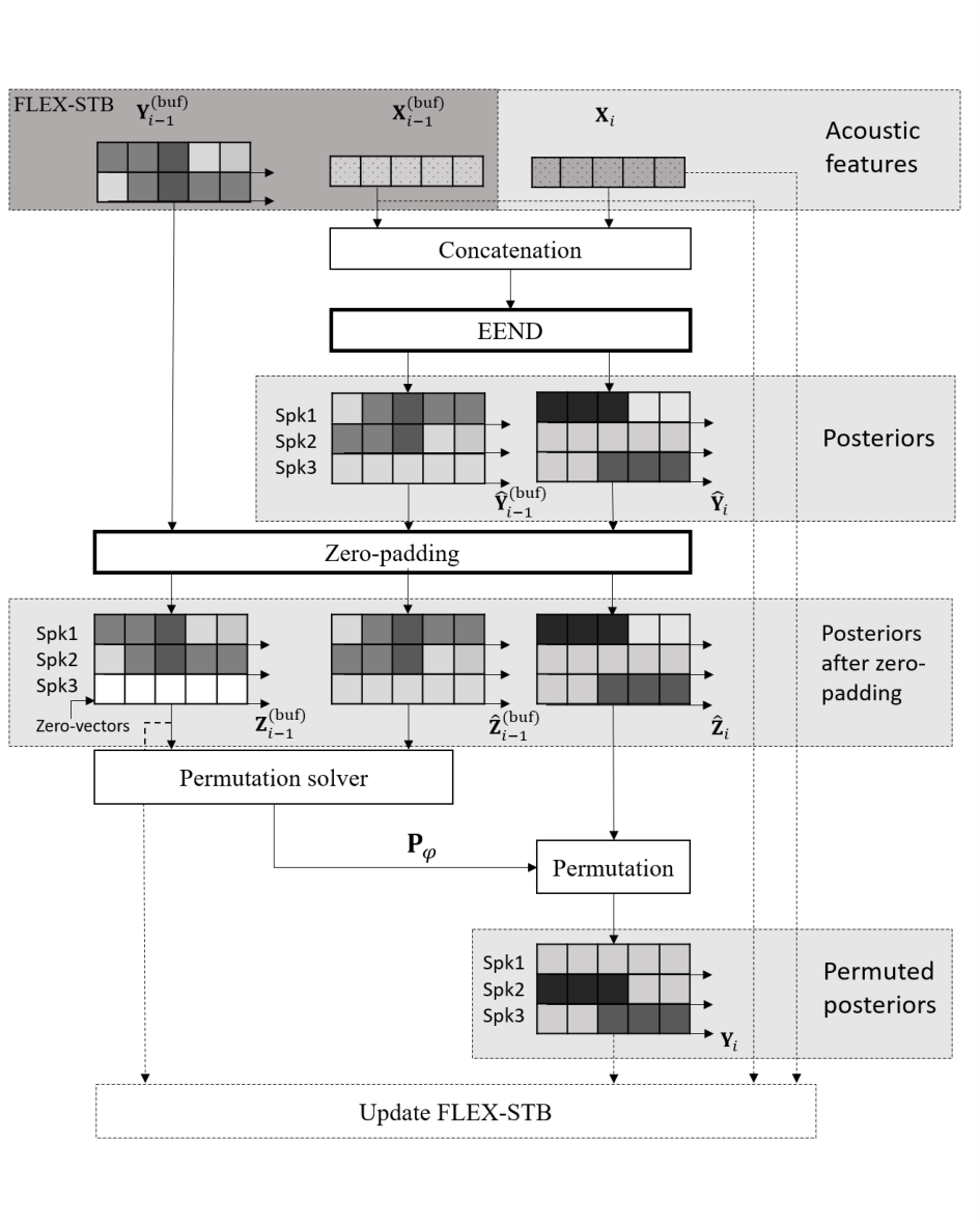
In this paper, we proposed the FLEX-STB which extends the STB coping with the two obstacles to use it with EEND for unknown numbers of speakers [30, 31]. The FLEX-STB deals with the varying number of speakers across chunks by increasing the number of speaker slots in the speaker-tracing buffer with the zero-padding in Section 3.1. When the system detects new speakers, it adds new zero-speaker-activity slots to the speaker buffer. We also propose four selection strategies to update the buffer, each of which are not limited by the number of speakers, in Section 3.2.
3.1 Speaker-tracing buffer for flexible numbers of speakers (FLEX-STB)
In this section, we assume that EEND estimates not only speech activities but also the number of speakers , i.e., . Firstly, to alleviate the different number of speakers between the buffer and the current chunk’s output , the posterior of the no-speech-activity speaker is considered as zero so that the zero-padding function is applied as follows:
| (8) | ||||
| (9) |
where and appends row zero vectors to so that the first dimension becomes . Next, the speaker permutation for the current chunk is calculated between and using Eq. (5). Then, the output for the current chunk is permuted as follows:
| (10) |
where is the final diarization result of the chunk . After that, at most time indexes are selected based on the concatenated outputs , and the FLEX-STB is updated as follows:
| (11) |
where is the -th column vector of , is the -th column vector of . The frame selection strategies are described in Section 3.2.
3.2 Selection strategy
When the number of accumulated features becomes larger than the buffer size , a selection strategy is needed to keep relevant features that contain the speaker permutation information from and . In this section, four selection functions are proposed for flexible numbers of speakers.
- •
Uniform sampling: Uniform distribution sampling is applied to extract frames.
- •
First-in-first-out (FIFO): The most recent features and the corresponding diarization results are stored in the buffer, which follows the first-in-first-out manner.
- •
Kullback-Leibler divergence based selection: We utilize the Kullback-Leibler divergence (KLD) to measure the difference between two probability distributions: the speaker activities distribution and the uniform distribution at time , which can be represented as follows:
(12) (13) (14) where is the posteriors from EEND with FLEX-STB and is the uniform distribution. Top samples with the highest KLD values are selected from and the corresponding .
- •
Weighted sampling using KLD: The combination of uniform sampling and KLD based selection. features are randomly selected with the probabilities which are proportional to .
| \toprule | Online () | |||||||
|---|---|---|---|---|---|---|---|---|
| \cmidrule(lr)2-7 | CALLHOME | DIHARD II | Offline () | |||||
| \cmidrule(lr)2-4\cmidrule(lr)5-7\cmidrule(l)8-9 | CALLHOME | DIHARD II | ||||||
| \cmidrule(r)1-7\cmidrule(l)8-9 FLEX-STB with selection strategy | ||||||||
| Uniform sampling | 27.6 | 20.2 | 19.3 | 52.4 | 39.3 | 36.8 | - | - |
| FIFO | 29.5 | 19.4 | 19.1 | 57.2 | 41.1 | 37.0 | - | - |
| KLD selection | 30.0 | 22.3 | 20.9 | 52.6 | 40.8 | 37.7 | - | - |
| Weighted sampling using KLD | 26.6 | 20.0 | 19.5 | 50.3 | 37.9 | 36.0 | - | - |
| \cmidrule(r)1-7\cmidrule(l)8-9 Without FLEX-STB | - | - | - | - | - | - | 15.3 | 32.9 |
| \bottomrule | ||||||||
4 Experiment
4.1 Data
We generated 100k simulated mixtures of one to four speakers following the procedure in [30] using Switchboard-2 (Phase I, II, III), Switchboard Cellular (Part 1, 1), and the NIST Speaker Recognition Evaluation datasets (SRE). Additionally, we added noises from the MUSAN corpus [38] and room impulse responses (RIRs) from the Simulated Room Impulse Response Database [39]. These simulated mixtures were used for training the EEND-based model. Two real conversation datasets: the CALLHOME [11] and the DIHARD II [3] were prepared for evaluation.
4.2 Experiment setting
In this paper, we evaluated the proposed method on the offline EEND-EDA model. The EEND-EDA model was trained with four Transformer encoder blocks and 256 attention units containing four heads [30]. We firstly trained the model using a two-speaker dataset for 100 epochs and then finetuned with the concatenation of one- to four-speaker simulated datasets for 25 epochs. Finally, EEND-EDA model was finetuned using a development set of CALLHOME, or DIHARD II, respectively.
We evaluated all systems with the diarization error rate (DER) metric in both overlapping and non-speech regions. A collar tolerance of 250 ms was applied at the start and end of each segment for the CALLHOME dataset. Following the regulation of the second DIHARD challenge [3], we did not use collar tolerance for the DIHARD II dataset.
4.3 Results
4.3.1 Effect of selection strategies and buffer size
Table 2 shows the effect of the selection strategies and the buffer size of the FLEX-STB on the EEND-EDA model in the left part. Experiment conditions varied from four selection methods with buffer sizes equal to , and but fixed the chunk size to . All results were calculated with the estimated number of speakers including the overlapping regions without oracle sound activity detection (SAD). It is shown that incremental buffer size which provides more input information improved the accuracy regardless of the selection strategies. Regarding the selection strategies, on most cases weighted sampling using KLD outperformed other strategies on both datasets. The best results from online system are and for CALLHOME and DIHARD II, respectively.
4.3.2 Comparison with the offline EEND-EDA system
We also compared the performance of our proposed online and baseline offline systems in Table 2. The input of the offline EEND-EDA system is the whole recording during inference while that for the online system is the chunk. Compared with the offline system, DERs of the online system increases by and on these two datasets, which would be acceptable degradation by considering the benefit of streaming diarization. The performance degradation is supposed to come from the mismatch between the offline model which was trained with fixed large chunk size and the online mechanism whose input sizes are incrementally increased.
4.3.3 Comparison with other online diarization systems
First, we compared our method with the recently proposed BW-EDA-EEND [34] on the CALLHOME dataset. In order to compare with BW-EDA-EEND in the same condition, we evaluated our method with a chunk size. As shown in Table 3, in a chunk size and estimated SAD condition, our proposed method outperforms the BW-EDA-EEND on all speaker-number cases on the CALLHOME dataset.
Next, we compared our proposed method with other systems in more realistic scenario, i.e., DIHARD II. For a fair comparison with other online methods, we follow the DIHARD II track 1, where the oracle SAD information is provided. We used the oracle SAD information to filter out non-speech frames of the estimated diarization result. Table 4 shows the comparison with other systems. The proposed online EEND-EDA with FLEX-STB achieved a DER of , which outperformed the UIS-RNN-SML, and is comparable to the offline DIHARD II baseline.
4.3.4 Real-time factor and latency
Our experiment was conducted on one NVIDIA Tesla P100 GPU. To calculate the average computing time of one buffer, we filled the buffer with dummy values for the first iteration to keep the buffer size always the same among chunks. The real-time factor was equal to 0.13 when we applied FLEX-STB to EEND-EDA with chunk size equal to , and a buffer size of . This means that the average computation duration of a chunk was which is acceptable for the online processing.
| \toprule | Number of speakers | ||
|---|---|---|---|
| \cmidrule(l)2-4 Method | 2 | 3 | 4 |
| \midruleBW-EDA-EEND [34] | 11.8 | 18.3 | 26.0 |
| EEND-EDA w/ FLEX-STB | 10.0 | 14.0 | 21.1 |
| \bottomrule | |||
5 Conclusion
In this paper, we proposed an online streaming speaker diarization method that handles overlapping speech and flexible numbers of speakers. A speaker tracing buffer for flexible numbers of speakers was proposed to mitigate the different number of speakers among chunks. Experimental results showed that the proposed online system achieves comparable results with the offline method and better results than the BW-EDA-EEND online method. One of our future studies is to incorporate various extensions developed at the recent DIHARD III challenge, including semi-supervised training and model fusion [6].
References
- [1] S. E. Tranter and D. A. Reynolds, “An overview of automatic speaker diarization systems,” IEEE Trans. on ASLP, vol. 14, no. 5, pp. 1557–1565, 2006.
- [2] X. Anguera, S. Bozonnet, N. W. D. Evans, C. Fredouille, G. Friedland, and O. Vinyals, “Speaker diarization: A review of recent research,” IEEE Trans. on ASLP, vol. 20, no. 2, pp. 356–370, 2012.
- [3] N. Ryant, K. Church, C. Cieri, A. Cristia, J. Du, S. Ganapathy, and M. Liberman, “The second DIHARD diarization challenge: Dataset, task, and baselines,” in INTERSPEECH, 2019, pp. 978–982.
- [4] N. Ryant, K. Church, C. Cieri, J. Du, S. Ganapathy, and M. Liberman, “Third DIHARD challenge evaluation plan,” arXiv preprint arXiv:2006.05815, 2020.
- [5] T. J. Park, N. Kanda, D. Dimitriadis, K. J. Han, S. Watanabe, and S. Narayanan, “A review of speaker diarization: Recent advances with deep learning,” arXiv preprint arXiv:2101.09624, 2021.
- [6] S. Horiguchi, N. Yalta, P. Garcia, Y. Takashima, Y. Xue, D. Raj, Z. Huang, Y. Fujita, S. Watanabe, and S. Khudanpur, “The Hitachi-JHU DIHARD III system: Competitive end-to-end neural diarization and x-vector clustering systems combined by DOVER-lap,” arXiv preprint arXiv:2102.01363, 2021.
- [7] W. Kang, B. C. Roy, and W. Chow, “Multimodal speaker diarization of real-world meetings using d-vectors with spatial features,” in ICASSP, 2020, pp. 6509–6513.
- [8] T. Yoshioka, I. Abramovski, C. Aksoylar, Z. Chen, M. David, D. Dimitriadis, Y. Gong, I. Gurvich, X. Huang, Y. Huang et al., “Advances in online audio-visual meeting transcription,” in ASRU, 2019, pp. 276–283.
- [9] J. Carletta, S. Ashby, S. Bourban, M. Flynn, M. Guillemot, T. Hain, J. Kadlec, V. Karaiskos, W. Kraaij, M. Kronenthal et al., “The AMI meeting corpus: A pre-announcement,” in MLMI, 2005, pp. 28–39.
- [10] A. Janin, D. Baron, J. Edwards, D. Ellis, D. Gelbart, N. Morgan, B. Peskin, T. Pfau, E. Shriberg, A. Stolcke et al., “The ICSI meeting corpus,” in ICASSP, vol. 1, 2003, pp. I–I.
- [11] “2000 NIST Speaker Recognition Evaluation,” https://catalog.ldc.upenn.edu/LDC2001S97.
- [12] A. Martin and M. Przybocki, “The NIST 1999 speaker recognition evaluation—an overview,” Digital signal processing, vol. 10, no. 1-3, pp. 1–18, 2000.
- [13] M. Senoussaoui, P. Kenny, T. Stafylakis, and P. Dumouchel, “A study of the cosine distance-based mean shift for telephone speech diarization,” IEEE Trans. on ASLP, vol. 22, no. 1, pp. 217–227, 2013.
- [14] J. Barker, S. Watanabe, E. Vincent, and J. Trmal, “The fifth “CHiME” speech separation and recognition challenge: Dataset, task and baselines,” in INTERSPEECH, 2018.
- [15] N. Kanda, R. Ikeshita, S. Horiguchi, Y. Fujita, K. Nagamatsu, X. Wang, V. Manohar, N. E. Y. Soplin, M. Maciejewski, S.-J. Chen et al., “The Hitachi/JHU CHiME-5 system: Advances in speech recognition for everyday home environments using multiple microphone arrays,” in CHiME-5, 2018.
- [16] S. Watanabe, M. Mandel, J. Barker, and E. Vincent, “CHiME-6 challenge: Tackling multispeaker speech recognition for unsegmented recordings,” in CHiME-6, 2020.
- [17] J. Geiger, F. Wallhoff, and G. Rigoll, “GMM-UBM based open-set online speaker diarization,” in INTERSPEECH, 2010.
- [18] K. Markov and S. Nakamura, “Improved novelty detection for online GMM based speaker diarization,” in INTERSPEECH, 2008.
- [19] S. Madikeri, I. Himawan, P. Motlicek, and M. Ferras, “Integrating online i-vector extractor with information bottleneck based speaker diarization system,” in INTERSPEECH, 2015, pp. 3105–3109.
- [20] D. Garcia-Romero, D. Snyder, G. Sell, D. Povey, and A. McCree, “Speaker diarization using deep neural network embeddings,” in ICASSP, 2017, pp. 4930–4934.
- [21] W. Zhu and J. Pelecanos, “Online speaker diarization using adapted i-vector transforms,” in ICASSP, 2016, pp. 5045–5049.
- [22] A. Zhang, Q. Wang, Z. Zhu, J. Paisley, and C. Wang, “Fully supervised speaker diarization,” in ICASSP, 2019, pp. 6301–6305.
- [23] E. Fini and A. Brutti, “Supervised online diarization with sample mean loss for multi-domain data,” in ICASSP, 2020, pp. 7134–7138.
- [24] M. Diez, L. Burget, S. Wang, J. Rohdin, and J. Černockỳ, “Bayesian HMM based x-vector clustering for speaker diarization,” in INTERSPEECH, 2019, pp. 346–350.
- [25] A. McCree, G. Sell, and D. Garcia-Romero, “Speaker diarization using leave-one-out gaussian PLDA clustering of dnn embeddings.” in INTERSPEECH, 2019, pp. 381–385.
- [26] Z. Huang, S. Watanabe, Y. Fujita, P. García, Y. Shao, D. Povey, and S. Khudanpur, “Speaker diarization with region proposal network,” in ICASSP, 2020, pp. 6514–6518.
- [27] Y. Fujita, N. Kanda, S. Horiguchi, K. Nagamatsu, and S. Watanabe, “End-to-end neural speaker diarization with permutation-free objectives,” in INTERSPEECH, 2019, pp. 4300–4304.
- [28] Y. Fujita, S. Watanabe, S. Horiguchi, Y. Xue, and K. Nagamatsu, “End-to-end neural diarization: Reformulating speaker diarization as simple multi-label classification,” arXiv preprint arXiv:2003.02966, 2020.
- [29] Y. Fujita, N. Kanda, S. Horiguchi, Y. Xue, K. Nagamatsu, and S. Watanabe, “End-to-end neural speaker diarization with self-attention,” in ASRU, 2019, pp. 296–303.
- [30] S. Horiguchi, Y. Fujita, S. Watanabe, Y. Xue, and K. Nagamatsu, “End-to-end speaker diarization for an unknown number of speakers with encoder-decoder based attractors,” in INTERSPEECH, 2020, pp. 269–273.
- [31] Y. Fujita, S. Watanabe, S. Horiguchi, Y. Xue, J. Shi, and K. Nagamatsu, “Neural speaker diarization with speaker-wise chain rule,” arXiv preprint arXiv:2006.01796, 2020.
- [32] T. von Neumann, K. Kinoshita, M. Delcroix, S. Araki, T. Nakatani, and R. Haeb-Umbach, “All-neural online source separation, counting, and diarization for meeting analysis,” in ICASSP, 2019, pp. 91–95.
- [33] K. Kinoshita, M. Delcroix, S. Araki, and T. Nakatani, “Tackling real noisy reverberant meetings with all-neural source separation, counting, and diarization system,” in ICASSP, 2020, pp. 381–385.
- [34] E. Han, C. Lee, and A. Stolcke, “BW-EDA-EEND: Streaming end-to-end neural speaker diarization for a variable number of speakers,” arXiv preprint arXiv:2011.02678, 2020.
- [35] Y. Takashima, Y. Fujita, S. Watanabe, S. Horiguchi, P. García, and K. Nagamatsu, “End-to-end speaker diarization conditioned on speech activity and overlap detection,” in SLT, 2021, pp. 849–856.
- [36] Y. Xue, S. Horiguchi, Y. Fujita, S. Watanabe, P. García, and K. Nagamatsu, “Online end-to-end neural diarization with speaker-tracing buffer,” in SLT, 2021, pp. 841–848.
- [37] Z. Dai, Z. Yang, Y. Yang, J. G. Carbonell, Q. Le, and R. Salakhutdinov, “Transformer-xl: Attentive language models beyond a fixed-length context,” in ACL, 2019, pp. 2978–2988.
- [38] D. Snyder, G. Chen, and D. Povey, “MUSAN: A music, speech, and noise corpus,” arXiv preprint arXiv:1510.08484, 2015.
- [39] T. Ko, V. Peddinti, D. Povey, M. L. Seltzer, and S. Khudanpur, “A study on data augmentation of reverberant speech for robust speech recognition,” in ICASSP, 2017, pp. 5220–5224.