Filling anomaly for general 2D and 3D symmetric lattices
Abstract
In this manuscript, we derive symmetry indicator formulas for the filling anomaly on 2D square lattices with and without time reversal, inversion symmetry, or their product, in the presence of spin-orbit coupling. We go beyond previous work by considering lattices with atoms occupying multiple Wyckoff positions. We also provide an algorithm using the Smith normal form that systematizes the derivation. The formulas determine the corner charge in 2D atomic or fragile topological insulators, as well as in 3D insulators and semimetals by studying their 2D slices. We apply our results to a 3D tight-binding model on a body-centered tetragonal lattice, whose projection into the 2D plane has two atoms in the unit cell. Our symmetry indicators correctly describe the higher-order hinge states and Fermi arcs in cases where the existing indicators do not apply.
I Introduction
The discovery of higher order topological insulators (HOTIs) has refined the notion of the bulk-boundary correspondence Benalcazar et al. 2017a; Schindler et al. 2018a; Song et al. 2017; Langbehn et al. 2017; Benalcazar et al. 2017b; Geier et al. 2018; Trifunovic and Brouwer 2019; Schindler et al. 2018b; Khalaf et al. 2018; Khalaf 2018; Ezawa 2018a; Ezawa 2018b; Matsugatani and Watanabe 2018; Imhof et al. 2018; Peterson et al. 2018; Serra-Garcia et al. 2018; Noh et al. 2018; You et al. 2018; Queiroz et al. 2019; Fang and Cano 2020. Specifically, an order- topological insulator in dimensions exhibits gapless modes on -dimensional surface, where corresponds to the usual bulk-boundary correspondence Schnyder et al. 2008; Schnyder et al. 2009; Kitaev 2009.
In this manuscript, we consider the case where . An order- topological insulator in dimensions exhibits zero-dimensional corner-localized mid-gap states Benalcazar et al. 2017b; Benalcazar et al. 2017a; Benalcazar et al. 2019; Schindler et al. 2019; Watanabe and Po 2020; Hirayama et al. 2020. Unlike a Chern insulator Panati 2007; Brouder et al. 2007, topological insulator Soluyanov and Vanderbilt 2011, or topological crystalline insulator Bradlyn et al. 2017; Po et al. 2017, an order- topological insulator in dimensions does not require an obstruction to the existence of symmetric, maximally localized Wannier functions. Instead, the corner charge can result from an obstructed atomic limit (OAL) phase Bradlyn et al. 2017, where the bulk is a band insulator that permits maximally localized and symmetric Wannier functions, but such that the Wannier centers cannot be continuously deformed into the positions of the atoms without breaking symmetry or closing the bulk (or surface Khalaf et al. 2019) band gap. This mismatch between the bulk atoms and Wannier centers has been dubbed the filling anomaly Benalcazar et al. 2019. In a symmetric finite-sized system at charge neutrality with no polarization or surface states, a filling anomaly results in a non-zero corner charge, quantized by crystal symmetry.
It is desirable to compute the filling anomaly and corner charge from bulk properties. To this end, there have been two recent approaches. The first, which applies to any lattice, regardless of symmetry, is to generalize the modern theory of polarization King-Smith and Vanderbilt 1993; Vanderbilt and King-Smith 1993; Resta 1994 by determining the corner charge from a bulk multipole moment Zhou et al. 2015; Wheeler et al. 2019; Kang et al. 2019; Ono et al. 2019; Trifunovic et al. 2019; Trifunovic 2020; Ren et al. 2020; Watanabe and Ono 2020. The second, which is taken in this manuscript, is to develop a theory of symmetry indicators, i.e., formulas derived in terms of the symmetry representations of the Bloch wavefunctions at high-symmetry momenta. Symmetry indicators have been very successful in classifying topological crystalline insulators Bradlyn et al. 2017; Vergniory et al. 2017; Elcoro et al. 2017; Po et al. 2017; Bradlyn et al. 2018; Cano et al. 2018; Khalaf et al. 2018; Song et al. 2018; Vergniory et al. 2019; Zhang et al. 2019; Cano and Bradlyn 2020 starting with the inversion eigenvalue formulas for 2D and 3D topological insulators Fu and Kane 2007.
Recently, symmetry indicators have been derived for the filling anomaly and corner charge in OALs in certain 2D crystals Benalcazar et al. 2019; Schindler et al. 2019. However, the results do not necessarily apply when there are multiple atoms in the unit cell. Specifically, Refs. Benalcazar et al. 2019; Schindler et al. 2019 limited their consideration to crystals for which there exists a symmetric finite-size termination containing an integer number of unit cells. Such a termination does not exist for a crystal with atoms occupying multiple distinct maximal Wyckoff positions. Instead, for such a crystal, all symmetric terminations contain a fractional number of unit cells, as shown in Fig. 1.

In this manuscript, we develop a method to compute symmetry indicators for the filling anomaly in the general case of a crystal with atoms occupying any number of Wyckoff positions. The method has two steps: we first compute the filling anomaly in terms of the number of Wannier functions centered at each Wyckoff position (which has also been done recently in Ref. Watanabe and Ono 2020). Second, we compute the number of Wannier centers at each Wyckoff position in terms of symmetry indicators using elementary band representations. The second step is accomplished via an algorithm that automates the calculation of symmetry indicators, introduced in this work. We apply our method to the square lattice with and without time reversal, inversion and their product, corresponding to the layer groups , , , , and ; the results are in Eqs. (23), (26), (32), (37), and (39), respectively. Our results provide a necessary generalization of formulas in previous work Benalcazar et al. 2019; Schindler et al. 2019, which can give an incorrect result when there are multiple atoms in the unit cell.
In addition to diagnosing band structures in 2D, the results of our work can be used to compute 2D invariants for slices of the 3D Brillouin zone, which is crucial to diagnosing the topology of 3D semimetals Wieder et al. 2020; Lin and Hughes 2018; Ghorashi et al. 2020 and some 3D HOTIs Song et al. 2017. We present an example of this in Sec. III.
The manuscript is organized as follows. In Sec. II, we review the concept of the filling anomaly and its connection to corner charge. We derive relations between the filling anomaly and the number of Wannier centers at each Wyckoff position. We then derive symmetry indicator formulas for the filling anomaly (and therefore corner charge) that apply to the square lattice.
In Sec. III, we build a 3D body-centered tetragonal (BCT) model. We analyze the HOTI phase and higher order semi-metal phase in this model by applying our formulas to each slice, which corresponds to a 2D system with two distinct atoms in the primitive unit cell. We verify our new formulas by numerically calculating the corner/hinge states. Our example demonstrates why the previous formulas in Refs. Benalcazar et al. 2019; Schindler et al. 2019 do not hold for a BCT lattice. In Sec. IV, we summarize our results and discuss future directions.
II 2D square lattice
We consider gapped 2D systems on the square lattice with no gapless edge modes and no bulk polarization. These systems are either (possibly obstructed) atomic limits or fragile topological phases, where all strong symmetry indicators vanish Po et al. 2017. In addition to the rotation symmetry of the square lattice, which we denote by , we consider the presence of time reversal , inversion , and/or their product, corresponding to the following 2D symmetry groups, known as layer groups: (, , ); (, ); (, ); (, ); and ( only), where the symmetry operations in parenthesis indicate the generators, excluding translations. The layer groups are listed in international notation, where indicates the rotation; indicates , indicates ; and indicates Litvin 2014. The layer group does not have a complete symmetry indicator formula, as pointed out in Ref. Schindler et al. 2019; we derive a partial indicator in Sec. II.5.4.
In this section, we describe the method for deriving the symmetry indicator for the filling anomaly (Secs. II.1, II.2 and II.3), which can be generalized to any crystal symmetry group in any dimension. In Sec. II.4, we apply the method to the symmetry group with spin-orbit coupling (SOC). We first re-derive the formula for the case of only one atom in the unit cell Schindler et al. 2019 and then derive a new formula for the situation where atoms occupy multiple Wyckoff positions. We generalize to the layer groups , , , and with SOC in Sec. II.5 and summarize in Sec. II.6.
II.1 Bulk-corner correspondence
Topologically trivial bands have symmetric and exponentially localized Wannier functions Bradlyn et al. 2017; Po et al. 2017. When the Wannier centers cannot be continuously moved to coincide with the atom positions while obeying crystal symmetry, the system is in an OAL phase Bradlyn et al. 2017. Despite having exponentially localized Wannier centers, OALs are non-trivial in the sense that they are separated by a gap-closing phase transition from the trivial phase (where the Wannier centers coincide with the atomic positions). Canonical examples include the Su-Schrieffer-Heeger model in 1D Su et al. 1979 and the quadrupole insulator in 2D Benalcazar et al. 2017b.
Due to the mismatch between the atomic positions and Wannier centers, OALs can sometimes support mid-gap corner-localized states. The connection between bulk Wannier centers and mid-gap corner charge is called the bulk-corner correspondence. The existence of mid-gap corner states indicates that in a finite-sized system with open boundaries, the number of filled bulk valence states is different from the filling required for charge neutrality. Thus, an OAL with mid-gap corner states can either be neutral or symmetric, but not both. This difference between the neutral and symmetric fillings is called the filling anomaly Benalcazar et al. 2019. A nontrivial filling anomaly requires not only that the number of filled states differs from the charge neutral filling, but also that the difference cannot be accounted for by adding or removing electrons to the boundary in a symmetry-preserving way. Thus, the filling anomaly remains robust even if the mid-gap states are pushed up(down) in energy into the conduction(valence) bands by a boundary potential.
In the symmetry groups with time-reversal ( and ), the filling anomaly is defined mod because one can add or remove eight electrons to the boundary of a finite-sized system without breaking these symmetries (by adding a Kramers pair of time-reversed partners to the four corners of a square lattice). In the systems without time-reversal (, , or ), the filling anomaly is defined mod because one can add four electrons to the boundary of a finite-sized system without breaking these symmetries, as electrons need not come in Kramers pairs.
In this work, we are interested in the filling anomaly that results from purely corner charge. Therefore, we limit ourselves to systems without gapless surface states, which excludes systems with a bulk polarization or a nontrivial topological invariant.
To compute the corner charge, we note that the symmetrically terminated square lattice with filling anomaly has net charge . Symmetry requires the charge is symmetrically sitting at the four corners, resulting in a corner charge on the square lattice Benalcazar et al. 2019,
| (1) |
Since, as discussed above, is defined either mod 8 or mod 4, it follows that is defined mod with time-reversal and mod without.
II.2 Defining the filling anomaly

We now derive the filling anomaly in terms of the ion positions and Wannier centers of the occupied valence bands. Both the ion positions and Wannier centers are described by Wyckoff positions; for a review of Wyckoff positions in the context of band theory, we refer the reader to Refs. Bradlyn et al. 2017; Cano et al. 2018. We use terminology specific to a finite square lattice of side length , but the method is general.
The first step is to count the number of electrons in the charge neutral configuration. To do this, we need to know the total number of ions in a finite-sized system with open boundary conditions. Let be one of the four Wyckoff positions on the 2D square lattice, , , , or , shown in Fig. 2. Define to be the number of ions at the Wyckoff position that reside inside or on the boundary of a finite-sized square consisting of unit cells. For a periodic lattice of size , the number of ions is multiplied by the multiplicity of the Wyckoff position. However, for open boundary conditions, this is not the case. As shown in Fig. 1(b), for an square with open boundary conditions:
| (2) |
The total number of electrons in the charge neutral configuration is then given by a sum over all Wyckoff positions:
| (3) |
where denotes the number of valence electrons from the ion at Wyckoff position . (More generally, if there are multiple ions not related by symmetry at the same Wyckoff position, which can happen for Wyckoff positions with a variable coordinate, such as the position, then should be the sum of valence electrons from each symmetry-distinct ion in the Wyckoff position .)
We now count the number of electrons required to symmetrically fill the Wannier centers of the valence bands in a finite-size system with open boundary conditions. Each Wannier center is labelled by a Wyckoff position, , and an irreducible representation (irrep), , of the site symmetry group of . (The site symmetry group of is the set of symmetry operations that leave invariant; therefore, Wannier functions centered at must transform as irreps of the site symmetry group. The irreps describe the symmetry of the Wannier functions.) Let count the number of Wannier functions centered at that transform as and are not related by symmetry; in the language of band representations Bradlyn et al. 2017; Cano et al. 2018, counts the number of times the band representation labelled by appears in the valence bands. Then the number of electrons needed to symmetrically fill the Wannier functions in a finite-size square with open boundary conditions is:
| (4) |
where is the dimension of the irrep .
Eqs. (3) and (4) define the filling anomaly:
| (5) |
where, as discussed in Sec. II.1, mod 8 applies with time-reversal symmetry and mod 4 applies without. Although this formula for includes an -dependent term on the right hand side, the -dependence disappears due to our assumptions that the system has no bulk charge polarization and no bulk net charge, which would contribute terms of order and , respectively. Thus, is independent of . A similar method to compute was used in Refs Schindler et al. 2019; Benalcazar et al. 2019; Watanabe and Ono 2020.
We now specify to the square lattice. The general Wyckoff position, denoted , has coordinates , where . Ions on the position always come in multiples of four, even on a finite size lattice, so that must be a multiple of four. Therefore, if time-reversal symmetry is absent, the term in Eq. (II.2) coming from the Wyckoff position is a multiple of four and does not contribute to the filling anomaly. If time-reversal symmetry is present, all electrons come in Kramers pairs, causing the term in Eq. (II.2) coming from the Wyckoff position to be a multiple of eight, which again does not contribute to the filling anomaly. Therefore, when computing the filling anomaly, we need only concern ourselves with the maximal Wyckoff positions , , and , shown in Fig. 2.
| Layer group | Site-symmetry group | |
|---|---|---|
| or | ||
|---|---|---|
A second simplification for the square lattice is that is independent of and for each symmetry group we consider, as we now explain. The maximal Wyckoff positions and their site symmetry groups are listed in Table 1 for all the layer groups we consider. In , Table 1 shows the only possible site-symmetry groups are or ; all irreps of these groups are two-dimensional, as shown in Table 2. The same is true for and . In , Table 1 shows the only possible site-symmetry groups are or ; all irreps of these groups are one-dimensional, as shown in Table 3. The same is true for ; its irreps are enumerated in Table 4.
Thus, in all cases, is independent of both and and the expression for in Eq. (II.2) can be simplified on the square lattice as,
| (6) |
where the sum is over all maximal Wyckoff positions ; is defined mod 4 (mod 8) in the absence (presence) of time-reversal symmetry, as in Eq. (II.2);
| (7) |
and
| (8) |
is the dimension of each irrep (which is independent of the choice of Wyckoff position and choice of irrep, as discussed in the previous paragraph.)
Plugging the formulas for from Eq. (II.2) into Eq. (6) yields:
| (9) |
where is defined mod 4 (mod 8) in the absence (presence) of time-reversal symmetry,
| (10) |
is the number of occupied bands, and is defined in Eq. (8).
The bulk charge is determined by the number scaling with in Eq. (9) and must be zero in a system that is charge neutral in the bulk:
| (11) |
The bulk polarization is determined by the number scaling with in Eq. (9) and must also be zero:
| (12) |
The filling anomaly is determined by the -independent term in Eq. (9):
| (13) |
where the equality follows from Eqs. (11) and (12). Equations (11), (12) and (13) were also obtained in Ref. Watanabe and Ono 2020.
II.3 Symmetry indicators for Wannier centers
The formulas in the previous section derive the filling anomaly in terms of the crystal structure and Wannier centers. We now derive in terms of the irreps of the little groups at high-symmetry points of the bulk band structure. This is useful because the irreps are easier to compute than the Wannier centers. As we will see, because the irreps in momentum space do not completely determine the Wannier centers Bacry et al. 1988; Michel and Zak 1992; Bacry 1993; Bradlyn et al. 2017; Cano and Bradlyn 2020; Cano et al. tion, can only be determined up to some modulus from symmetry.
To this end, let be the integer “EBR matrix” of the symmetry group under consideration: each column of is labelled by an EBR and each row a particular irrep of the little group of a particular high-symmetry point. The entries in the matrix indicate the number of times each momentum space irrep appears in the EBR Song et al. 2020a; Song et al. 2020b; Cano and Bradlyn 2020.
A group of topologically trivial bands can be expressed as a linear combination of EBRs Bradlyn et al. 2017 with integer coefficients . The irreps that appear at high-symmetry points in the band structure satisfy
| (14) |
where is the number of times the irrep appears in the band structure. We need to invert this equation to find in terms of , as we now explain.
Let the Smith normal form of be given by
| (15) |
where is a diagonal integer matrix with diagonal entries , i.e., the first entries are positive and the remaining entries are zero, and are integer matrices invertible over the integers. (Note: the stable topological crystalline insulator classification of the group is given by , where is the group of integers mod Po et al. 2017; Song et al. 2018; Song et al. 2020a; Song et al. 2020b; Cano and Bradlyn 2020.)
We want to express the number of EBRs corresponding to each Wyckoff position in terms of symmetry irreps. Since we are only considering topologically trivial bands, we consider only the vectors for which there exists an integer vector that solves Eq. (14). Then the Smith normal form in Eq. (15) implies , where divides . For such bands, one solution to Eq. (14) is given by , where is the pseudoinverse of , i.e., a diagonal matrix with diagonal entries . This solution is not generically unique: the most general solution to Eq. (14) is , where is any integer vector in the nullspace of , i.e., the first entries of are zero, so that . Thus, given a particular , can only be determined modulo , where gcd indicates the greatest common divisor.
However, we do not need each separately: we seek in Eq. (7), which is a sum of all where the EBR indicated by is induced from an irrep of the site-symmetry group of the Wyckoff position ; we use to denote this set of EBRs. Then, following the previous paragraph, we can express as
| (16) |
We now use Eq. (16) to compute in in terms of the symmetry indicators. We do the same for , , , and in Sec. II.5. The Smith normal form of the EBR matrix for each of these groups is computed in Appendix A.
II.3.1 Symmetry indicators for in
In , there are three high-symmetry points in the Brillouin zone: , and . The point is symmetry-related to , so does not add any new information. The points and are invariant under the point group , while is invariant under ; the irreps of both groups are listed in Table 2.
Define () to be the number of times the irrep () appears in the valence band spectrum at the high-symmetry point and define . Similarly, define to be the number of times the irrep appears in the valence band spectrum at . Then define to be the difference between the number of times the irrep indicated by appears at the high-symmetry point and at :
| (17) |
Using this notation, we find from Eq. (16) (details in Appendix A):
| (18) | |||||
| (19) | |||||
| (20) |
where is the total number of filled bands, which was derived by imposing bulk charge neutrality in Eq. (11).
II.4 Symmetry indicators for the filling anomaly
We are now ready to compute the filling anomaly in Eq. (6) in terms of the symmetry irreps by plugging in Eqs. (18), (19), and (20) for the group (the results for other groups are in Sec. II.5). In previous work Benalcazar et al. 2019; Schindler et al. 2019, was computed on 2D lattices with only one maximal Wyckoff position occupied. The main advance of this work is to compute for square lattices with any number of atoms in the unit cell. In Sec. II.4.1, we compute for the simple square lattice with one atom in the unit cell, reproducing earlier results Schindler et al. 2019. In Sec. II.4.2, we derive in the general case with multiple atoms in the unit cell.
II.4.1 Simple square lattices
We now reproduce the symmetry indicator formula in Ref. Schindler et al. 2019 for a square lattice with one atom in the unit cell. Without loss of generality, we can take that atom to be in the position. Then the formula for the filling anomaly in Eq. (13) (with ) simplifies to
| (21) |
Plugging the expression for in Eq. (19) into Eq. (21), we obtain the symmetry indicator formula:
| (22) |
Noticing that must be an even number in an (obstructed) atomic limit phase because in Eq. (20) must be an integer, we deduce that is in fact a quantity. Eq. (22) was introduced in Eq. (50) in Ref. Schindler et al. 2019.
II.4.2 General case: atoms in multiple Wyckoff positions
We now consider the general case, shown in Fig. 1(b), where there can be atoms at any Wyckoff positions. Thus, the number of electrons from each ion, , can all be non-zero. The number of filled bands is . Plugging Eq. (18) into the expression for the filling anomaly in Eq. (13) (with ) we find the symmetry indicator formula for the filling anomaly:
| (23) |
Since time-reversal symmetry constrains and to be even numbers and, as discussed below Eq. (22), is also even, the filling anomaly is again a quantity. When , which implies , Eq. (23) is equivalent to Eq. (22) (to see this, notice that the equations are mod 8, is even, and when , Eq. (12) implies , from which Eqs. (19) and (20) together require that is also even.) When , Eq. (23) is distinct from Eq. (22) and has not appeared in previous literature.
In Sec. III, we build an explicit body-centered tetragonal model with , and symmetry. The Hamiltonian in the and planes of the model describes a square lattice with symmetry, but with atoms at multiple Wyckoff positions, corresponding to the projection of the 3D model onto a 2D plane. Therefore, the 2D bulk-corner correspondence derived in this section applies to 2D planes of that model, providing a numerical check of the analytical results.
II.5 Generalization to other layer groups
We now compute the filling anomaly in terms of the symmetry indicators for the layer groups , , and and explain why does not have an analogous formula. The formulas for in this section are derived in Appendix A.
II.5.1
For the layer group , the high-symmetry points and are invariant under the point group , while is invariant under . The irreps for these groups are listed in Table 2. The number of Wannier centers at each Wyckoff position, , and , are defined by Eq. (7) with irrep dimension in Eq. (8). Using Eq. (16), we find and can be determined mod :
| (24) | |||||
| (25) |
where , where indicates the number of times the irrep appears in the valence bands at the high-symmetry point . We find mod 1, i.e., is not constrained by symmetry irreps.
The filling anomaly is determined by Eq. (13) taken mod 4 with . Substituting in Eq. (24) yields:
| (26) |
where the subscript is to distinguish the filling anomaly in from that computed in in Eq. (23). In the case where atoms only occupy one Wyckoff position (), and this equation reduces to
| (27) |
Eq. (27) was introduced in the context of higher order Fermi arcs Wieder et al. 2020 with and symmetries: the anti-commuting reflection symmetries there play the same role as in in generating two dimensional irreps.
II.5.2
For the layer group , the high-symmetry points and are invariant under the point group , while is invariant under ; the irreps for these groups are listed in Table 3. The number of Wannier centers at each Wyckoff position, , and , are defined by Eq. (7) with irrep dimension in Eq. (8). Using Eq. (16), we find that and can be determined mod , while can be determined mod :
| (28) | ||||
| (29) | ||||
| (30) |
Here we use the notation , where corresponds to the irrep with eigenvalue , and , , where corresponds to the irrep with eigenvalues , . As in previous sections, indicates the number of times the irrep appears in the valence bands at the high-symmetry point .
II.5.3
For the layer group , the high-symmetry points and are invariant under the point group , while is invariant under ; the irreps for these groups are listed in Table 4. The number of Wannier centers at each Wyckoff position, , and , are defined by Eq. (7) with irrep dimension in Eq. (8). From Eq. (16), we find that and can be determined mod while can be determined mod . The formulas are:
| (33) | ||||
| (34) | ||||
| (35) |
Here we use the notation , where the irrep of labelled by has eigenvalue , , and inversion eigenvalue corresponding to . In addition, and , where , correspond to the irreps of with eigenvalues , and inversion eigenvalues corresponding to . We denote .
II.5.4
The group does not have a symmetry indicator formula, as we now explain. The filling anomaly is given by Eq. (13) taken mod 8 with (from Eq. (8)):
| (38) |
However, is given by Eq. (24) (as explained in Appendix A.5, the symmetry indicator formula for is the same in as in ) and is only defined mod 2. It follows from plugging Eq. (24) into Eq. (38) that the symmetry indicator formula for is only defined mod 4, even though should be determined mod 8. Thus, we say that the symmetry indicator formula does not exist because the symmetry indicators do not provide enough information to completely determine the filling anomaly in this group. The mod 8 filling anomaly can only be partially determined mod 4:
| (39) |
II.6 Summary of 2D results
Eqs. (23), (26), (32), and (37) are the symmetry indicator formulas that express the filling anomaly in OALs in terms of the symmetry invariants. Together, these formulas encompass all square lattices with time-reversal, inversion symmetry, and/or their product, and any number of atoms in the unit cell.
All the formulas derived in this section are additive, and can be applied to an insulating band structure with any number of filled valence bands, as long as it is charge neutral, polarization free, and all the strong symmetry indicators are trivial. Because of the additivity, the formulas also apply to fragile topological phases, as discussed in Ref. Benalcazar et al. 2017b.
We now discuss some connections to previous work. As we have mentioned earlier, the formulas for the filling anomaly in Refs. Benalcazar et al. 2019 and Schindler et al. 2019 do not accommodate multiple atoms in the unit cell. In Ref. Watanabe and Ono 2020, the filling anomaly was computed in terms of in the general case of having multiple atoms in the unit cell, but was not expressed in terms of the symmetry indicators. Finally, the real space invariants computed in Ref. Song et al. 2020b are related to the computed here and are computed using the EBR matrix, but there is not a one-to-one correspondence between them. Ref. Kooi et al. 2020 also discusses real space topological invariants that go beyond symmetry indicators.
In Appendix B, we derive the symmetry indicator formula for the filling anomaly for a finite-sized square lattice with a boundary normal to the direction. It turns out that the formulas are the same as we have derived in this section, where the boundary is normal to the direction. The results in this section can be generalized to a finite-sized square lattice with a boundary normal to any direction by defining a square supercell with a side parallel to the boundary. Since the supercell necessarily contains multiple atoms, the results in Sec. II.4.2 apply; in order to get the correct irreps at high-symmetry points, the band structure must be computed relative to the supercell. Non-square terminations can also obey symmetry (for example, an octagon); while the general logic described in this section applies, the counting in Eq. (II.2) will be different.
Interestingly, we have found numerically that the corner states survive even if the global symmetry is broken, i.e., in a square lattice with an integer number of unit cells. Although rigorously the corner states are not protected if the lattice symmetry is broken globally, physically this makes sense because the localized states on one corner should not depend on how the lattice is terminated at other corners. A different method to compute the presence of gapless boundary states in other systems with a fractional number of unit cells was discussed in Ref. Rhim et al. 2018.

III 3D model on the body-centered tetragonal lattice
We now apply the results derived in the previous section to classify the topology of a 3D tight-binding Hamiltonian. We are interested in the HOTI and higher order Fermi arc (HOFA) phases. The topology of these phases can be understood by studying 2D slices of the Brillouin zone with fixed . For example, the HOTI phase can be viewed as Wannier center pumping between the two time-reversal invariant planes ( and ) Song et al. 2017, while the HOFA phase requires each 2D fixed- slice on the Fermi arc to have a non-trivial filling anomaly Wieder et al. 2020. The difference between the previous works and the present manuscript is that we consider a symmetric body-centered tetragonal (BCT) model, whose 2D slices in momentum space necessarily contain atoms at different Wyckoff positions, as we will show in the next section. Therefore, the results obtained in Sec. II.4.2 and II.5 are necessary to correctly identify the filling anomaly of 2D slices in momentum space.
III.1 Tight-binding model
We build an explicit BCT tight-binding model in space group () with a spin- degree of freedom on each site. The space group is generated by body-centered lattice translations, a rotation about the -axis, inversion, and time-reversal symmetry. The matrix forms of these generators are given below in terms of the spin- generators, (whose matrix forms are defined in Appendix C) and decomposed into Pauli matrices and :
| (40) | ||||
| (41) | ||||
| (42) |
where is complex conjugation. It will be convenient to introduce .
We define a Cartesian coordinate system by the unit vectors , , , where and are lattice constants. We align the base of the conventional tetragonal unit cell diagonally with respect to the and axes (see Fig. 3(a)). In this basis, the primitive translation vectors of the BCT lattice are given by , , . The conventional unit cell has two atoms, indicated by solid and hollow circles in Fig. 3(a), which form two sublattices. The primitive unit cell has one atom.
We take the lattice constants . Therefore, each atom has four nearest neighbors on the same sublattice and eight next-nearest neighbors on the opposite sublattice. Our model only includes hopping between each site and these 12 nearest and next-nearest neighbors, illustrated in Fig. 3(a). One of each of these hopping terms is given below (and drawn in Fig. 3(a)) and the others are related by symmetry:
| (43) |
The symmetry-related hopping terms in other directions are written explicitly in Appendix. D. There is also an onsite mass term:
| (44) |
The parameters , , and are real, and is complex; is the complex conjugate of . The Hamiltonian is written in momentum space in both the primitive and conventional bases in Appendix D.
III.2 Topological phases
We now classify the topology of this model by considering the Hamiltonian in 2D slices of the 3D Brillouin zone. Specifically, for fixed , can be regarded as the Hamiltonian of a 2D system. Since eigenstates generically have weight on both sublattices, this 2D Hamiltonian describes atoms on a square lattice with two sites in the unit cell, as shown in Fig. 3(b). If the 2D Hamiltonian has no gapless edge states or polarization, then we can apply our results from Sec. II.4.2 and II.5 to determine the corner charge of this 2D model when the 3D system is truncated in the and directions but infinite in the direction.
We find that our model has several topological phases depending on the ratio . The parameters and do not change the topological phase. We list all the different phases in Fig. 3(e) with respect to : there is one HOTI phase and two Dirac semimetal (DSM) phases, which we now describe.
III.2.1 HOTI
| 0 | 2 | 4 | 1 | 0 | 0 | 1 | 1 | 0 | 0 |
| 2 | 4 | -1 | 0 | 0 | 3 | -1 | 0 | 4 |
When , a HOTI with the non-trivial symmetry indicator is realized. This phase was introduced in Refs. Song et al. 2017; Khalaf et al. 2018. While all the -slices are either atomic limits or fragile phases in 2D, the 3D phase is stable topological because the 2D Wannier centers move as a function of , which leads to helical modes on 1D hinges where the - and -normal surfaces meet.
Here, we derive this 3D phase on the BCT lattice by computing the filling anomaly in the and planes. Since these two planes are invariant under time reversal, they are described by the layer group , for which we derived the symmetry indicator formula for the filling anomaly in Eq. (23) of Sec. II.4.
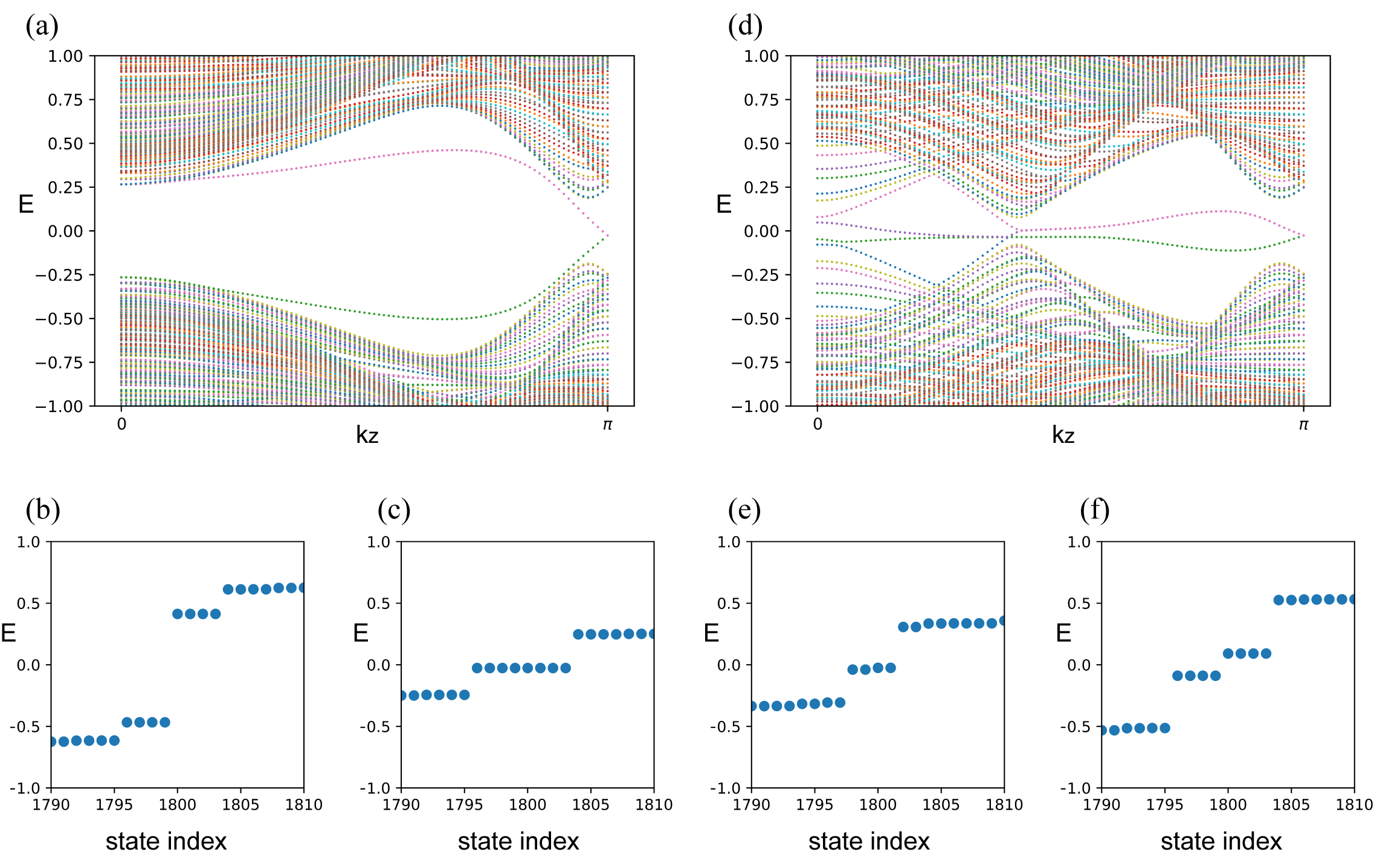
The symmetry indicators are shown in Table 5, from which the filling anomaly can be computed with Eq. (23). We find that in the plane and in the plane. The non-trivial value in the plane is responsible for the eight-fold degenerate mid-gap states we observe in Fig. 3(c) in the plane for a finite-size rod geometry, which is finite in the - and -directions and infinite in the direction. Since in the plane, to continuously connect the mid-gap states with the rest of the band structure requires -dependent modes that traverse the bulk band gap; these are exactly the helical hinge modes required by the 3D HOTI phase. Interestingly, Table 5 shows that ; thus, this slice is a fragile topological 2D insulator. (This by itself is not enough to show that the slice is fragile because are only defined mod 4 (and mod 2); some algebra shows that there is no solution where .)
We now reiterate the importance of our analysis in correctly describing this phase: our formula (23) correctly captures the filling anomaly in the plane (and lack of filling anomaly in the plane), which agrees with both our numerical results and the helical edge modes predicted by the 3D formula in Ref. Song et al. 2017. Earlier formulas for the filling anomaly give an incorrect result. Specifically, Eq. (22) of Ref. Schindler et al. 2019 yields in the plane and in the plane. This discrepancy occurs because Ref. Schindler et al. 2019 does not accommodate atoms at multiple Wyckoff positions. While and are consistent with a helical mode, they do not agree with the state counting in our numerics, where there is always the same number of occupied and empty bands (and hence only consistent with and , as we correctly obtain from Eq. (23)).
III.2.2 HOFA in Dirac Semimetals
| 2 | 4 | 0 | 2 | 0 | 0 | 2 | |
| 2 | 4 | 1 | 1 | 1 | 0 | 0 |
When , the model is in one of two DSM phases and has two Dirac points along in the bulk. The band structure for the DSM(i) phase on a rod finite in the - and -directions and infinite in is shown in Fig. 3(d). For both of the phases, there are HOFA hinge states connecting the projection of the two bulk Dirac points. The HOFA hinge states pass through , where there are also projected gapless mirror Chern surface states. The difference between the two phases is that the phase DSM(i) has filling anomaly mod 8 at while the plane in phase DSM(ii) is trivial.
The HOFA hinge states occur in the planes between the two Dirac points. Since these planes are not time-reversal invariant, but are invariant under the product of time-reversal and inversion, they are described by the layer group , for which we derived the symmetry indicator formula for the filling anomaly in Eq. (26) of Sec. II.5.1. Applying this formula, we find in the planes between the bulk Dirac points, as derived in Table 6.
The HOFA are not correctly described by formulas in previous work derived by assuming atoms at only one maximal Wyckoff position: for example, Eq. (27) yields in these planes, which would indicate a lack of hinge modes.
In the DSM(i) phase, besides the HOFA, there are two groups of corner-localized hinge states that cross at . These states can be pushed into the valence or conduction bands by adding some symmetry protecting potentials, however the filling anomaly at remains non-trivial. These states are not present in the DSM(ii) phase which has in the plane.
Further, we note that the gapless surface states at are unavoidable, even if the protecting mirror symmetry is broken, because the HOFA states are four fold degenerate while the only possible degeneracy of mid gap states at a time-reversal symmetric plane is eight (corresponding to a Kramers pair of time-reversed partners at each corner.) This discrepancy between the HOFA degeneracy and the required degeneracy at can only be resolved by having gapless surface or bulk states projected to the point.
IV discussion
In this manuscript, we introduced a general method to derive the symmetry indicator formula for the filling anomaly that applies to crystals with any number of atoms in the unit cell. We introduced an algorithm using the Smith normal form that makes the derivation systematic. We applied this method to derive the filling anomaly on the 2D square lattice with time-reversal, inversion, and/or their product. We further showed where our results go beyond earlier work that did not apply to crystals with atoms occupying multiple maximal Wyckoff positions.
We verified our results by correctly predicting the helical hinge modes and HOFAs in a 3D BCT tight-binding model, by analyzing 2D slices of the Brillouin zone. This model served as a concrete example where previous results break down, showing the importance of our extension to crystals with atoms in multiple maximal Wyckoff positions.
Our method can be easily generalized to other () symmetric 2D lattices and higher dimensional lattices. It will also be interesting to apply our results to other topological semimetals, such as those in Bradlyn et al. 2016 which occur on non-symmorphic lattices and therefore necessarily have multiple atoms in the unit cell.
Note added. During the final stages of this work, Ref. Takahashi et al. 2021 appeared on the ArXiv, which also computes the filling anomaly in terms of symmetry indicators for general lattices with symmetry. Our results agree where they overlap.
Acknowledgements.
This material is based upon work supported by the National Science Foundation under Grant No. DMR-1942447. J.C. acknowledges the support of the Flatiron Institute, a division of the Simons Foundation.References
- Benalcazar et al. (2017a) W. A. Benalcazar, B. A. Bernevig, and T. L. Hughes, Electric multipole moments, topological multipole moment pumping, and chiral hinge states in crystalline insulators, Physical Review B 96, 245115 (2017a).
- Schindler et al. (2018a) F. Schindler, A. M. Cook, M. G. Vergniory, Z. Wang, S. S. Parkin, B. A. Bernevig, and T. Neupert, Higher-order topological insulators, Science advances 4, eaat0346 (2018a).
- Song et al. (2017) Z. Song, Z. Fang, and C. Fang, (d- 2)-dimensional edge states of rotation symmetry protected topological states, Physical review letters 119, 246402 (2017).
- Langbehn et al. (2017) J. Langbehn, Y. Peng, L. Trifunovic, F. von Oppen, and P. W. Brouwer, Reflection-symmetric second-order topological insulators and superconductors, Physical review letters 119, 246401 (2017).
- Benalcazar et al. (2017b) W. A. Benalcazar, B. A. Bernevig, and T. L. Hughes, Quantized electric multipole insulators, Science 357, 61 (2017b).
- Geier et al. (2018) M. Geier, L. Trifunovic, M. Hoskam, and P. W. Brouwer, Second-order topological insulators and superconductors with an order-two crystalline symmetry, Phys. Rev. B 97, 205135 (2018).
- Trifunovic and Brouwer (2019) L. Trifunovic and P. W. Brouwer, Higher-order bulk-boundary correspondence for topological crystalline phases, Physical Review X 9, 011012 (2019).
- Schindler et al. (2018b) F. Schindler, Z. Wang, M. G. Vergniory, A. M. Cook, A. Murani, S. Sengupta, A. Y. Kasumov, R. Deblock, S. Jeon, I. Drozdov, et al., Higher-order topology in bismuth, Nature physics 14, 918 (2018b).
- Khalaf et al. (2018) E. Khalaf, H. C. Po, A. Vishwanath, and H. Watanabe, Symmetry indicators and anomalous surface states of topological crystalline insulators, Phys. Rev. X 8, 031070 (2018).
- Khalaf (2018) E. Khalaf, Higher-order topological insulators and superconductors protected by inversion symmetry, Phys. Rev. B 97, 205136 (2018).
- Ezawa (2018a) M. Ezawa, Minimal models for wannier-type higher-order topological insulators and phosphorene, Phys. Rev. B 98, 045125 (2018a).
- Ezawa (2018b) M. Ezawa, Higher-order topological insulators and semimetals on the breathing kagome and pyrochlore lattices, Phys. Rev. Lett. 120, 026801 (2018b).
- Matsugatani and Watanabe (2018) A. Matsugatani and H. Watanabe, Connecting higher-order topological insulators to lower-dimensional topological insulators, Phys. Rev. B 98, 205129 (2018).
- Imhof et al. (2018) S. Imhof, C. Berger, F. Bayer, J. Brehm, L. W. Molenkamp, T. Kiessling, F. Schindler, C. H. Lee, M. Greiter, T. Neupert, and R. Thomale, Topolectrical-circuit realization of topological corner modes, Nature Physics 14, 925 (2018).
- Peterson et al. (2018) C. W. Peterson, W. A. Benalcazar, T. L. Hughes, and G. Bahl, A quantized microwave quadrupole insulator with topologically protected corner states, Nature 555, 346 (2018).
- Serra-Garcia et al. (2018) M. Serra-Garcia, V. Peri, R. Süsstrunk, O. R. Bilal, T. Larsen, L. G. Villanueva, and S. D. Huber, Observation of a phononic quadrupole topological insulator, Nature 555, 342 (2018).
- Noh et al. (2018) J. Noh, W. A. Benalcazar, S. Huang, M. J. Collins, K. P. Chen, T. L. Hughes, and M. C. Rechtsman, Topological protection of photonic mid-gap defect modes, Nature Photonics 12, 408 (2018).
- You et al. (2018) Y. You, T. Devakul, F. J. Burnell, and T. Neupert, Higher-order symmetry-protected topological states for interacting bosons and fermions, Phys. Rev. B 98, 235102 (2018).
- Queiroz et al. (2019) R. Queiroz, I. C. Fulga, N. Avraham, H. Beidenkopf, and J. Cano, Partial lattice defects in higher-order topological insulators, Phys. Rev. Lett. 123, 266802 (2019).
- Fang and Cano (2020) Y. Fang and J. Cano, Higher-order topological insulators in antiperovskites, Physical Review B 101, 245110 (2020).
- Schnyder et al. (2008) A. P. Schnyder, S. Ryu, A. Furusaki, and A. W. Ludwig, Classification of topological insulators and superconductors in three spatial dimensions, Physical Review B 78, 195125 (2008).
- Schnyder et al. (2009) A. P. Schnyder, S. Ryu, A. Furusaki, and A. W. Ludwig, Classification of topological insulators and superconductors, in AIP Conference Proceedings, Vol. 1134 (American Institute of Physics, 2009) pp. 10–21.
- Kitaev (2009) A. Kitaev, Periodic table for topological insulators and superconductors, in AIP conference proceedings, Vol. 1134 (American Institute of Physics, 2009) pp. 22–30.
- Benalcazar et al. (2019) W. A. Benalcazar, T. Li, and T. L. Hughes, Quantization of fractional corner charge in -symmetric higher-order topological crystalline insulators, Physical Review B 99, 245151 (2019).
- Schindler et al. (2019) F. Schindler, M. Brzezińska, W. A. Benalcazar, M. Iraola, A. Bouhon, S. S. Tsirkin, M. G. Vergniory, and T. Neupert, Fractional corner charges in spin-orbit coupled crystals, Physical Review Research 1, 033074 (2019).
- Watanabe and Po (2020) H. Watanabe and H. C. Po, Fractional corner charge of sodium chloride, arXiv preprint arXiv:2009.04845 (2020).
- Hirayama et al. (2020) M. Hirayama, R. Takahashi, S. Matsuishi, H. Hosono, and S. Murakami, Higher-order topological crystalline insulating phase and quantized hinge charge in topological electride apatite, Phys. Rev. Research 2, 043131 (2020).
- Panati (2007) G. Panati, Triviality of bloch and bloch–dirac bundles, Annales Henri Poincaré 8, 995 (2007).
- Brouder et al. (2007) C. Brouder, G. Panati, M. Calandra, C. Mourougane, and N. Marzari, Exponential localization of wannier functions in insulators, Phys. Rev. Lett. 98, 046402 (2007).
- Soluyanov and Vanderbilt (2011) A. A. Soluyanov and D. Vanderbilt, Wannier representation of topological insulators, Phys. Rev. B 83, 035108 (2011).
- Bradlyn et al. (2017) B. Bradlyn, L. Elcoro, J. Cano, M. Vergniory, Z. Wang, C. Felser, M. Aroyo, and B. A. Bernevig, Topological quantum chemistry, Nature 547, 298 (2017).
- Po et al. (2017) H. C. Po, A. Vishwanath, and H. Watanabe, Symmetry-based indicators of band topology in the 230 space groups, Nature communications 8, 1 (2017).
- Khalaf et al. (2019) E. Khalaf, W. A. Benalcazar, T. L. Hughes, and R. Queiroz, Boundary-obstructed topological phases, arXiv preprint arXiv:1908.00011 (2019).
- King-Smith and Vanderbilt (1993) R. D. King-Smith and D. Vanderbilt, Theory of polarization of crystalline solids, Phys. Rev. B 47, 1651 (1993).
- Vanderbilt and King-Smith (1993) D. Vanderbilt and R. King-Smith, Electric polarization as a bulk quantity and its relation to surface charge, Physical Review B 48, 4442 (1993).
- Resta (1994) R. Resta, Macroscopic polarization in crystalline dielectrics: the geometric phase approach, Reviews of modern physics 66, 899 (1994).
- Zhou et al. (2015) Y. Zhou, K. M. Rabe, and D. Vanderbilt, Surface polarization and edge charges, Phys. Rev. B 92, 041102 (2015).
- Wheeler et al. (2019) W. A. Wheeler, L. K. Wagner, and T. L. Hughes, Many-body electric multipole operators in extended systems, Phys. Rev. B 100, 245135 (2019).
- Kang et al. (2019) B. Kang, K. Shiozaki, and G. Y. Cho, Many-body order parameters for multipoles in solids, Phys. Rev. B 100, 245134 (2019).
- Ono et al. (2019) S. Ono, L. Trifunovic, and H. Watanabe, Difficulties in operator-based formulation of the bulk quadrupole moment, Physical Review B 100, 245133 (2019).
- Trifunovic et al. (2019) L. Trifunovic, S. Ono, and H. Watanabe, Geometric orbital magnetization in adiabatic processes, Phys. Rev. B 100, 054408 (2019).
- Trifunovic (2020) L. Trifunovic, Bulk-and-edge to corner correspondence, Physical Review Research 2, 043012 (2020).
- Ren et al. (2020) S. Ren, I. Souza, and D. Vanderbilt, Quadrupole moments, edge polarizations, and corner charges in the wannier representation (2020), arXiv:2010.13862 [cond-mat.mes-hall] .
- Watanabe and Ono (2020) H. Watanabe and S. Ono, Corner charge and bulk multipole moment in periodic systems, Phys. Rev. B 102, 165120 (2020).
- Vergniory et al. (2017) M. Vergniory, L. Elcoro, Z. Wang, J. Cano, C. Felser, M. Aroyo, B. A. Bernevig, and B. Bradlyn, Graph theory data for topological quantum chemistry, Physical Review E 96, 023310 (2017).
- Elcoro et al. (2017) L. Elcoro, B. Bradlyn, Z. Wang, M. G. Vergniory, J. Cano, C. Felser, B. A. Bernevig, D. Orobengoa, G. Flor, and M. I. Aroyo, Double crystallographic groups and their representations on the bilbao crystallographic server, Journal of Applied Crystallography 50, 1457 (2017).
- Bradlyn et al. (2018) B. Bradlyn, L. Elcoro, M. Vergniory, J. Cano, Z. Wang, C. Felser, M. Aroyo, and B. A. Bernevig, Band connectivity for topological quantum chemistry: Band structures as a graph theory problem, Physical Review B 97, 035138 (2018).
- Cano et al. (2018) J. Cano, B. Bradlyn, Z. Wang, L. Elcoro, M. Vergniory, C. Felser, M. Aroyo, and B. A. Bernevig, Building blocks of topological quantum chemistry: Elementary band representations, Physical Review B 97, 035139 (2018).
- Song et al. (2018) Z. Song, T. Zhang, Z. Fang, and C. Fang, Quantitative mappings between symmetry and topology in solids, Nature communications 9, 1 (2018).
- Vergniory et al. (2019) M. Vergniory, L. Elcoro, C. Felser, N. Regnault, B. A. Bernevig, and Z. Wang, A complete catalogue of high-quality topological materials, Nature 566, 480 (2019).
- Zhang et al. (2019) T. Zhang, Y. Jiang, Z. Song, H. Huang, Y. He, Z. Fang, H. Weng, and C. Fang, Catalogue of topological electronic materials, Nature 566, 475 (2019).
- Cano and Bradlyn (2020) J. Cano and B. Bradlyn, Band representations and topological quantum chemistry, arXiv preprint arXiv:2006.04890 (2020).
- Fu and Kane (2007) L. Fu and C. L. Kane, Topological insulators with inversion symmetry, Physical Review B 76, 045302 (2007).
- Wieder et al. (2020) B. J. Wieder, Z. Wang, J. Cano, X. Dai, L. M. Schoop, B. Bradlyn, and B. A. Bernevig, Strong and fragile topological dirac semimetals with higher-order fermi arcs, Nature communications 11, 1 (2020).
- Lin and Hughes (2018) M. Lin and T. L. Hughes, Topological quadrupolar semimetals, Phys. Rev. B 98, 241103 (2018).
- Ghorashi et al. (2020) S. A. A. Ghorashi, T. Li, and T. L. Hughes, Higher-order Weyl Semimetals, arXiv e-prints , arXiv:2007.02956 (2020), arXiv:2007.02956 [cond-mat.mes-hall] .
- Litvin (2014) D. B. Litvin, 1-, 2- and 3-Dimensional Magnetic Subperiodic Groups and Magnetic Space Groups (2014) https://www.iucr.org/publ/978-0-9553602-2-0.
- Su et al. (1979) W. P. Su, J. R. Schrieffer, and A. J. Heeger, Solitons in polyacetylene, Phys. Rev. Lett. 42, 1698 (1979).
- Altmann and Herzig (1994) S. L. Altmann and P. Herzig, Point-group theory tables (Oxford, 1994).
- Bacry et al. (1988) H. Bacry, L. Michel, and J. Zak, Symmetry and analyticity of energy bands in solids, Phys. Rev. Lett. 61, 1005 (1988).
- Michel and Zak (1992) L. Michel and J. Zak, Physical equivalence of energy bands in solids, EPL (Europhysics Letters) 18, 239 (1992).
- Bacry (1993) H. Bacry, Duals of crystallographic groups. band and quasi-band representations, Commun. Math. Phys. 153, 359 (1993).
- Cano et al. (tion) J. Cano, L. Elcoro, M. I. Aroyo, B. A. Bernevig, and B. Bradlyn, (In preparation.).
- Song et al. (2020a) Z.-D. Song, L. Elcoro, Y.-F. Xu, N. Regnault, and B. A. Bernevig, Fragile phases as affine monoids: classification and material examples, Physical Review X 10, 031001 (2020a).
- Song et al. (2020b) Z.-D. Song, L. Elcoro, and B. A. Bernevig, Twisted bulk-boundary correspondence of fragile topology, Science 367, 794 (2020b).
- Kooi et al. (2020) S. H. Kooi, G. van Miert, and C. Ortix, Bulk-corner correspondence of time-reversal symmetric insulators: deduplicating real-space invariants, arXiv preprint arXiv:2008.07345 (2020).
- Rhim et al. (2018) J.-W. Rhim, J. H. Bardarson, and R.-J. Slager, Unified bulk-boundary correspondence for band insulators, Physical Review B 97, 115143 (2018).
- Bradlyn et al. (2016) B. Bradlyn, J. Cano, Z. Wang, M. Vergniory, C. Felser, R. Cava, and B. A. Bernevig, Beyond dirac and weyl fermions: Unconventional quasiparticles in conventional crystals, Science 353 (2016).
- Takahashi et al. (2021) R. Takahashi, T. Zhang, and S. Murakami, General corner charge formula in two-dimensional -symmetric higher-order topological insulators, (2021), arXiv:2101.04322 [cond-mat.mes-hall] .
- Fang et al. (2012) C. Fang, M. J. Gilbert, and B. A. Bernevig, Bulk topological invariants in noninteracting point group symmetric insulators, Physical Review B 86, 115112 (2012).
Appendix A Symmetry indicator formulas for the number of occupied EBRs at each Wyckoff position
In this Appendix, we explain how the formulas for in the main text are derived from the Smith normal form.
A.1
We first consider the group . The band representations induced from the three maximal Wyckoff positions , , and (shown in Fig. 2) are listed in Table 7. Each band representation is expressed as a vector in the basis:
| (45) |
where indicates the number of times the irrep occurs at the high-symmetry point in the momentum-space band representation. Note and are invariant under , while is invariant under ; their irreps are defined in Table 2.
Each group of topologically trivial bands, isolated in energy from all other bands, can be written as an integer linear combination of EBRs. The coefficients form a vector in the following basis:
| (46) |
where indicates the number of times the EBR induced from the two dimensional irrep of the site-symmetry group of the Wyckoff position appears in the linear combination. In this basis, we use Table 7, which lists all EBRs and their momentum space irreps, to construct the EBR matrix defined in Sec. II.3:
| (47) |
Each column of indicates the momentum space irreps of a particular EBR, where the columns are ordered according to the list of EBRs in (46) and the rows are ordered according to the list of momentum space irreps in (45). For example, the first column corresponds to the band representation induced by and the first entry, “1”, indicates that the irrep appears one time in this EBR (as listed in Table 7).
Following Sec. II.3, we apply the Smith decomposition to the EBR matrix :
| (48) |
where and , which are invertible over integers, are found to be:
| (49) |
| (50) |
and the diagonal matrix is
| (51) |
The eighth entry, 4, which is the only non-zero, non-unity entry of , indicates the symmetry indicator classification of this group Po et al. 2017. The zero entries impose the constraint that an insulator must have the same number of occupied bands at all high-symmetry points.
To see this last point, consider a vector in the basis of Eq. (45), which satisfies for some integer vector that represents a sum of EBRs in the basis of Eq. (46). According to the Smith decomposition in Eq. (48), . Since the ninth and tenth entries on the diagonal of are zero, it follows that . Plugging in the entries of from Eq. (49) and using the basis of in Eq. (45) yields two equations:
| (52) |
The first line specifies that there must be the same number of occupied bands at as at and the second line specifies that there must be the same number of occupied bands at and at .
The pseudoinverse of is
| (53) |
We can now plug , , and into Eq. (16) to find in Eqs. (18), (19) and (20).
Physically, the ambiguity in the modulus of comes from the fact that the Wannier centers are not gauge invariant; this point is elaborated on in Ref. Song et al. 2020b. For example, one can check (by using ) that the irreps at high-symmetry points for the band representations represented by , and are identical. This corresponds to the fact that the Wannier centers for these three band representations can all be continuously moved to the general Wyckoff position without breaking symmetries. Therefore, they are physically indistinguishable by symmetry indicators.
A.2
The group contains and symmetries, but not or separately. A basis for its irreps and EBRs can be read from the previous subsection by forgetting about inversion symmetry. Specifically, the basis for the irrep labels in momentum space is:
| (54) |
which is the same as Eq. (45) without the labels for the inversion eigenvalue, and the basis for the multiplicity of each EBR is:
| (55) |
which is the same as Eq. (46) without the labels. The EBR matrix is:
| (56) |
The Smith decomposition (Eq. (48)) yields the matrices:
| (57) |
| (58) |
| (59) |
A.3
In the case of , the site-symmetry groups of the maximal Wyckoff positions are defined in Table 1 and their irreps are defined in Table 3. The basis of irreps in momentum space is:
| (60) |
The basis of EBRs is:
| (61) |
Then the EBR matrix is
| (62) |
Notice this EBR matrix in Eq. (62) is identical to Eq. (47), although their bases have different meanings. We again use Eq. (16) to find the symmetry indicator formulas for , and in Eqs. (28), (29), and (30).
A.4
In the case of layer group , the site-symmetry groups of the maximal Wyckoff positions are defined in Table 1 and their irreps are defined in Table 4. The basis of momentum space irreps is:
| (63) |
The basis of EBRs is:
| (64) |
Then the EBR matrix is:
| (65) |
After Smith decomposition (Eq. (48)), the diagonal matrix is:
| (66) |
and
| (67) |
The matrix is too unwieldy to present here.
A.5
In , the site-symmetry groups of the maximal Wyckoff positions are listed in Table 1. Table 2 shows that their irreps are identical to those of . Thus, the EBR matrix and its Smith normal form is the same as for in Sec. A.2 and and are given by Eqs. (24) and (25), respectively, while is determined only modulo one.
Appendix B Filling anomaly when the boundary is rotated by relative to the unit cell

We derive an expression for the filling anomaly for a finite square lattice whose boundaries are rotated relative to the primitive unit cell, as shown in Fig. 4. We consider the general case where there may be atoms at any number of Wyckoff positions (shown in Fig. 4(b)); the case where there is only one Wyckoff position occupied by atoms (shown in Fig. 4(a)) is a special case.
The Wyckoff positions are defined with respect to the primitive unit cell. To compute the filling anomaly, we need only consider the maximal Wyckoff positions, as we argued in Sec. II.2. The donated electrons from each maximal Wyckoff position are denoted by , , and . The number of filled bands is .
The number of atoms, , at each Wyckoff position in this terminated square lattice with atoms along each side is given by
| (68) |
(Notice these are different than in Eq. (II.2), where is computed with the boundary parallel to the unit cell.) From Eqs. (6) and (B), we find the filling anomaly:
| (69) |
The bulk charge is determined by the number scaling with in this expression and must be zero:
| (70) |
where we have used the expression for in Eq. (10). The bulk polarization parallel to the boundaries is determined by the coefficient of . Since we are interested in polarization-free systems, the term proportional to must vanish:
| (71) |
The last term in Eq. (71) vanishes mod 4 or mod 8. In addition, the last term in Eq. (70) clearly vanishes mod 4, but also vanishes when taken mod 8, which applies in the presence of time-reversal symmetry, because time-reversal requires that be even and ( is defined in Eq. (8).) Thus, the only constraint from Eqs. (70) and (71) is
| (72) |
Notice that this constraint differs from the constraint in Eq. (12), which applies when the boundary is parallel to the unit cell. As a result need not be even, as we found in Table 5.
The filling anomaly is determined by the -independent term:
| (73) |
where we have simplified the -independent term from Eq. (69) by taking it mod 4 (or mod 8). Notice Eq. (73) is identical to Eq. (13), which is derived for the case where the boundary is parallel to the unit cell. Therefore, the symmetry indicators will be the same in the two cases.
Appendix C Spin-3/2 matrices
Appendix D Details of BCT tight-binding model
In this appendix, we provide additional details about the BCT model studied in Sec. III. The BCT model has the symmetry of space group , as well as time-reversal symmetry .
The unit cell and hoppings are illustrated in Figs. 3(a) and (b). The model includes hopping to the four nearest and eight next-nearest (if ) atoms. The relation between the two hopping terms shown in Eq. (43) and the other ten hopping terms are:
| (86) |
and
| (87) |
where the matrix forms of the symmetry generators are given in Eqs. (40), (41) and (42), and .
The primitive lattice has one site in the unit cell. Since each site has a spin- degree of freedom, the Hamiltonian, defined by Eqs. (43), (86), and (87) is a matrix, given by:
| (88) |
where , , correspond to the momenta reciprocal to , , .
D.1 Hamiltonian and symmetry operators in conventional unit cell
The conventional unit cell contains two sublattices, as indicated in Fig. 3(a). Since each site hosts a spin- degree of freedom, the Hamiltonian in the conventional unit cell in reciprocal space is an matrix, which takes the form
| (89) |
where again , , correspond to the basis reciprocal to , , , and we have introduced an additional set of Pauli matrices to indicate the sublattice degree of freedom. As in the main text and in the Hamiltonian in Eq. (D), and act on the hybrid spin and orbital degrees of freedom.
D.2 Parameters for numerical calculations
There is an unexpected anti-unitary symmetry in the plane. This symmetry is artificial because it can be broken by adding small next-next-nearest hopping terms that preserve all the symmetries. The extra terms do not change the topology and do not break any symmetry, but will help to eliminate unphysical gapless surface states which are protected by the artificial symmetry. These small next-nearest hopping terms are:
| (91) |
We consider a system that is finite in the and directions, i.e., its boundaries are normal to and , as shown in Fig. 3(b). We terminate the boundary to respect symmetry.
In our numerical calculations, the parameters are set to be: , , , . The parameters are taken in such a way that when , there is a quadratic band touching at . The rod states are calculated for a square of size by . In Fig. 3(c), , realizing the HOTI phase. In Fig. 3(d), , realizing the DSM(i) phase.
The phase diagram in Fig. 3(e) is derived with . This small value of only slightly changes the phase transition points of .
D.3 Symmetry eigenvalues in the HOTI phase and DSM(i) phase
| HSP | ||||
|---|---|---|---|---|
| 2 | 0 | 0 | 0 | |
| 1 | 1 | 0 | 0 | |
| 1 | 0 | 1 | 0 | |
| 1 | 1 | 0 | 0 | |
| 2 | 0 | 0 | 0 | |
| 0 | 1 | 1 | 0 |
| HSP | ||||||
|---|---|---|---|---|---|---|
| 1 | 0 | 1 | 0 | 1 | 1 | |
| 1 | 1 | 0 | 0 | 2 | 0 | |
| 1 | 0 | 1 | 0 | 1 | 1 | |
| 2 | 0 | 0 | 0 | 2 | 0 | |
| 1 | 1 | 0 | 0 | 2 | 0 | |
| 0 | 1 | 1 | 0 | 1 | 1 |
We list the the symmetry eigenvalues computed from our model in the HOTI phase in Table 8. The results are used to calculate the filling anomaly in Table 5.
The symmetry eigenvalues computed in the DSM(i) phase are listed in Table 9. The results are used to calculate the filling anomaly in Table 6. In addition, the plane has mirror Chern number . The mirror Chern number can be evaluated by calculating the Chern numbers of the and sectors. The symmetry indicator formula for the Chern number is Fang et al. 2012:
| (92) |
where is twice the total spin and can be replaced with the number of filled bands in our spinful case; is the eigenvalue of the band; and is the eigenvalue of the band. Time-reversal symmetry ensures that the number of filled band in each mirror sector is . Time-reversal symmetry also constrains the mirror Chern number: . We can determine by counting the numbers of irreps that contain mirror eigenvalue and plug them into Eq. (92). For example, has two components: and . Since this irrep has inversion eigenvalue , only the eigenvalue corresponds to the sector with mirror eigenvalue . Thus, in Eq. (92). The other irreps come into the equation similarly. From these facts, we obtain the symmetry indicator formula for the mirror Chern number for our layer group at this plane (, and ):
| (93) |
Plugging in the symmetry eigenvalues from Table 8, we find at , and at . For the HOTI phase, the mirror Chern number for both and planes, as we can verify by plugging the symmetry eigenvalues from Table 9 into Eq. (D.3).
There are a pair of bulk Dirac points at . The symmetry eigenvalues at a -plane between and can be obtained by ”forgetting” the inversion eigenvalues of , and . The symmetry eigenvalues at a -plane between and can be obtained by ”forgetting” the inversion eigenvalues of , and .
D.4 Numerical calculation for a rod geometry with integer number of unit cells

The corner states are protected by the global symmetry. Thus, rigorously, a -symmetric termination of the lattice is required to protect the corner states. However, in practice we find that the corner states survive on a lattice termination that is not globally -symmetric if it has symmetry in the bulk (see Fig. 5 for an example of such a lattice termination). Physically, this is reasonable because if the corners are far apart, the local spectrum at one corner should not depend on the termination at another corner.
In Fig. 6, we numerically compute the rod states of our model with the same parameters as in App. D.2 (, , , ), but with an integer number of unit cells, breaking the global symmetry. The spectrum is similar to Fig. 3(c) and (d) (where global symmetry is preserved) for the same system size. Most importantly, the filling anomalies of each slice (obtained by counting the number of occupied bands) for the two choices of terminations are the same.