Viscometry of electron fluids from symmetry
Abstract
When electrons flow as a viscous fluid in anisotropic metals, the reduced symmetry can lead to exotic viscosity tensors with many additional, non-standard components. We present a viscometry technique that can in principle measure the multiple dissipative viscosities allowed in isotropic and anisotropic fluids alike. By applying representation theory to exploit the intrinsic symmetry of the fluid, our viscometry is also exceptionally robust to both boundary complications and ballistic effects. We present the technique via the illustrative example of dihedral symmetry, relevant in this context as the point symmetry of 2D crystals. Finally, we propose a present-day realizable experiment for detecting, in a metal, a novel hydrodynamic phenomenon: the presence of rotational dissipation in an otherwise-isotropic fluid.
Introduction—Hydrodynamics models the transport of conserved quantities, such as charge or energy, over large length- and time-scales. In ultra-pure low-temperature metals, electronic momentum can also be approximately conserved, if the collisions that conserve momentum are much faster than those that relax it (e.g. off impurities or via umklapp) lucasreview17. In these viscous electron fluids, hydrodynamic effects can give rise to exotic transport phenomena, such as decreasing resistance with increasing temperature (Gurzhi effect) gurzhi and superballistic constriction flow levitov1607.
Theorized for many decades, electron hydrodynamics has in recent years garnered compelling experimental evidence molenkamp; crossno; bandurin; kumar2017superballistic; bandurin18; bakarov; imaging1; imaging2; imaging3. The earliest discoveries of electron hydrodynamics took place in GaAs molenkamp, monolayer graphene crossno, and bilayer graphene bandurin. At low (but non-zero) charge density, these are all isotropic Fermi liquids well-described by Galilean-invariant, textbook hydrodynamics landau. For the electron fluid in graphene, the shear viscosity – the sole dominant viscosity in this isotropic Fermi liquid – has been both calculated polini1506; NarozhnyVisc and indirectly measured in experiment bandurin; kumar2017superballistic; imaging2.
Metals are generically anisotropic, however, as the presence of a crystalline lattice explicitly breaks rotational symmetry. Indeed, experiments and ab initio calculations have recently suggested hydrodynamics might apply in less symmetric metals, e.g. gooth2018thermal, fu2018thermoelectric, mop2019, vool2020imaging. In such cases, anisotropy leads to a number of novel phenomena varnavides2020electron, including rotational viscosity cook2019 and intrinsic Hall viscosity Toshio_2020. Such viscosities are inaccessible to current experiments, however, as existing methods (non-local resistances polini; levitovhydro, constriction conductances levitov1607, AC phenomena CorbinoVisc, current imaging imaging1; imaging2; imaging3, channel flows link, and heat transport vignale; gooth2018thermal; heatTransport1; heatTransport2) (i) are not robust to boundary and ballistic effects, and (ii) cannot distinguish all the symmetry-allowed viscosities that will generically appear.
Here, we present a multi-terminal device, robust to both boundary complications and ballistic effects, that can measure the multiple dissipative viscosity components allowed in isotropic and anisotropic fluids, all on a single sample. Our viscometry relies on the representation theory of point groups, from which we devise boundary conditions that isolate viscosities via symmetry-constrained heating. Our technique is also uniquely capable detecting a “smoking gun” signal of a novel hydrodynamic phenomenon: the isolated emergence of rotational viscosity in an “otherwise isotropic” fluid cook2019.
Strikingly, rotational viscosity gives viscous dissipation even under rigid rotations of a fluid, which is forbidden by angular momentum conservation in isotropic fluids, but generically allowed in anisotropic fluids. For hexagonal fluids in particular, emerges in a novel and isolated way cook2019, alongside only the standard, isotropic shear and bulk viscosities. Hexagonal electron fluids therefore provide a highly novel setting for finding , with possible candidate materials including mackenzie, wang2020goniopolar, and -trilayer graphene Zibrov_2018. Finally, we argue that our viscometry proposed here is in fact the only feasible way of discovering in an electron fluid.
In what follows, we describe our viscometry via the illustrative example of 2D fluids of dihedral point symmetry. However, our approach extends naturally to fluids of higher dimension and/or differing point symmetry.
Dihedral hydrodynamics—The dihedral group is the -element group of symmetries of the regular -gon. As an abstract group, is generated by its elements , a ()-rotation about the -gon center, and , a reflection through a fixed axis containing the -gon center, with . We also take to be the group of symmetries of the circle, which includes rotations of arbitrary angle. By the crystallographic restriction theorem ashcroft, the paradigmatic 2D electron fluids are those of dihedral point symmetry.
In Newtonian fluids (appropriate for the linear response regime lucasreview17), viscous stresses arise linearly in response to velocity gradients , with proportionality given by the viscosity tensor . In the Supplemental Material (SM), we show that any -invariant viscosity tensor must take the form
| (1) |
where is the Levi-Civita symbol and are Pauli matrices. We have excluded in Eq. 1 only the viscosity tensor; in such fluids, one has eight allowed viscosities, not all of which are isolated by our viscometry due to the exceptionally-low symmetry of . We therefore relegate discussion of this singular case to SM.
We emphasize that the presence of rotational viscosity in Eq. 1 does not rely on electrons or dihedral symmetry: it is universal to anisotropic fluids. The lack of rotational symmetry allows the stress tensor to have a non-vanishing antisymmetric component , which in the hydrodynamics must couple to the strain tensor component of the same symmetry (i.e. the vorticity); this generic coupling is . Fig. 1 illustrates the microscopic origin of in anisotropic electron fluids.
The remaining viscosities appearing in Eq. 1 can be understood as follows: bulk viscosity bulkFN couples the trace of the stress tensor to the fluid expansion , plus viscosity couples the stress along the axes of the crystal to the strain , and cross viscosity couples stress and strain at 45∘ to the crystal axes. Equating plus and cross viscosities in the tensor () gives the tensor (), and further taking in the tensor gives the isotropic tensor (). We therefore discuss dihedral viscosities without further loss of generality by henceforth assuming the case.
We now turn to the linearized (i.e. assuming Stokes flow lucasreview17; landau) hydrodynamics. For fluids, the hydrodynamic equations are the following pair of approximate conservation laws:
| (2a) | ||||
| (2b) | ||||
where () is the (equilibrium) fluid density, the electronic speed of sound, and is the rate of momentum-relaxing collisions. Eq. 2a describes the local conservation of density , with an associated conserved current . The current has a convective contribution from the fluid momentum and a diffusive contribution , with the incoherent diffusion constant cook2019; hartnoll1. Eq. 2b describes the approximate conservation of fluid momentum in the presence of viscous and ohmic forces.
One may in principle append to Eq. 2 a third conservation law for energy. At , this complication does not qualitatively modify the dynamics of homogeneous electron fluids lucasreview17. At (e.g. the Dirac fluid of charge-neutral graphene), the energy density couples to velocity in an analogous way to charge density in Eq. 2. Due to this analogy we focus on the case, but our results are generalizable to Dirac fluids.

We now restrict to static flows , so that the left-hand-side of Eq. 2 vanishes. We can then automatically satisfy the resulting divergence-free condition on 2a by writing the current in terms of a stream function: Using this stream function , we eliminate density from the (static) momentum equation 2b and, neglecting terms of order , we find that the stream function satisfies the generalized biharmonic equation
| (3) |
where we have introduced the parameters
| (4) |
and non-dimensionalized all lengths , , using an assumed measurement lengthscale (which will later characterize the size of our viscometer). Using an assumed solution of the generalized biharmonic 3, we solve for in Eq. 2b, which tells us that (away from ) the current is approximately coherent at this order incFN. Substituting this result into the stream function relation, we find that the fluid is approximately incompressible: .
The parameter 4 is known as the Gurzhi length and characterizes the length-scale past which momentum-relaxing effects begin to dominate viscous effects lucasreview17. The dimensionless parameter 4 characterizes the degree of square anisotropy in the fluid and must lie in the interval . The transformation corresponds to a rotation of the crystal coordinates by , and implies (no square anisotropy in the fluid).
Dihedral viscometry—Our dihedral viscometer is a square , with current boundary conditions consisting of contacts, each of width , on its perimeter. Contacts are placed in pairs symmetrically about the midpoint of each edge, separated from each other by a tunable spacing . A total current is either injected or drained at each contact, with the configuration of the viscometer determined by these choices. For concreteness, we take box function contacts boxFN, and no-slip at the boundary away from contacts, in all numerical calculations (though our main results are unaffected by such details).
Our viscometry functions by exploiting the spatial symmetry of the dissipation generated in the fluid. The viscous dissipation is best understood via the irreducible symmetries of the -invariant viscosity tensor, which we now outline; see SM for details.
Informally, a group representation tung allows a group to act on a vector space, by assigning group elements to matrices in a way that is consistent with the underlying group multiplication. For finite groups and complex vector spaces, any such representation can be decomposed into a sum of elementary, “building-block” representations, known as irreducible representations (irreps). The dihedral group has five irreps: four -dimensional representations (the superscript denotes reflection parity, , and the subscript denotes rotation parity, ) and one -dimensional vector representation cook2019; tung. These irreps label the five irreducible ways a mathematical object can self-consistently transform under reflection and 4-fold rotation. The irreps of and their realizations as current boundary conditions on a square are summarized in Table 1.
Particularly relevant for viscometry is the -dimensional vector space of rank-2 tensors, as the velocity strain tensor is an element of this space: . The viscosity tensor then acts linearly on as a matrix by index contraction. Since the viscosity tensor is -invariant, Schur’s lemma tung implies that must act proportionally to the identity on each -invariant subspace of . We illustrate this result by expressing the heat that is generated through viscous dissipation, , as
| (5) | ||||
where each term in Eq. 5 represents a projection of into a given 1-dimensional -invariant subspace of , corresponding to a -dimensional irrep of .
Note that the total totalFN heat generated by the fluid flow also contains an ohmic contribution . Even though is not a component of the viscosity tensor, the fluid velocity nevertheless transforms according to the remaining vector irrep , conveniently completing our correspondence between irreps and dissipative coefficients in Table 1.
Importantly, both the center of the square and its boundary are mapped to themselves under any symmetry transformation. Thus the center strain tensor and center velocity must have the same symmetry as the square boundary. This implies that we can selectively isolate at the square center each of the terms in the heat decomposition by choosing boundary conditions corresponding to each of the irreps of .
The above considerations are summarized in Table 1. A numerical demonstration of isolated , , and heating is given in Fig. 2 (see SM for additional flow plots). In SM, we further show that our result does not fundamentally rely on hydrodynamics; across the entire ballistic-to-hydrodynamic crossover, our symmetry-based “viscometer” continues to isolate dissipation channels according to their symmetry.

The isolated center heat generated solely by the viscosity sources a Poisson equation crossno
| (6) |
for temperature , with the electronic thermal conductivity. If one is able to measure both the center temperature variation (e.g. by local thermometry zhang2017anomalous; diamondTempSensing) and center strain component (e.g. by flow imaging imaging1; imaging2; imaging3), then can be determined. Alternatively, if one uses only local thermometry, one may still estimate – and hence – by mapping out heating patterns via Eq. 6 and comparing against numerical simulations.
Another consistency check arises by varying the viscometer geometry. Numerically solving Eq. 3 for varying contact spacing , we show in Fig. 3 how the anisotropy can be determined experimentally. The center heat (as a function of contact spacing ) varies uniquely with anisotropy , allowing for computation of the latter. In fact, we show in SM how may be determined from as few as contact spacings and boundary configurations, for total center heat measurements.
Finally, in SM we discuss how our viscometry compares against more conventional Poiseuille, channel flow methods, particularly in the case link where there is insufficient symmetry to isolate all viscosities via boundary conditions, as above.
Conclusions—Even if the above procedure cannot be carried out in full, one may nevertheless detect rotational viscosity by simply observing center heat in the configuration. -symmetry precludes any center heat that might arise from another viscosity component, ohmic effects, incoherent currents, or even ballistic scattering (in addition to being highly suppressed in the viscous limit, ballistic center heat also has easily distinguishable scaling with viscometer size ; see SM). We therefore anticipate that our viscometry can enable the discovery of in the near future.
We further claim that (in contrast to other dihedral viscosities) there is no feasible way to detect beyond the symmetry-based technique proposed here. Expanding the hexagonal viscosity tensor 1 in Eq. 2b, one in fact obtains the isotropic momentum equation, but with replacements vectorCalcFN. This implies that rotational viscosity does not modify bulk flow patterns. Although exotic no-stress boundary conditions can in principle generate weakly -dependent flows, the incomplete understanding of viscous electron boundary conditions makes it is unclear how such an experiment could be robustly carried out.

Indeed, there has been much discussion concerning the proper boundary conditions (e.g. no-slip, no-stress, generalized Robin) for viscous electron flow wagner2015boundary; kiselev2019boundary; moessner2019boundary. Because our viscometer relies on symmetry, it conveniently side-steps any such boundary complication, so long as the boundaries are symmetrically complicated. For example, although we assumed no-slip boundary conditions in the preceeding numerics, if no-stress or generalized Robin boundary conditions are instead required, the numerical values in Figs. 2 and 3 will change but the irrep decomposition of the rank-2 tensor space will continue to guarantee isolated center heating.
We emphasize that our viscometry extends to more general fluids. For fluids of point group symmetry , one constructs a device with -irreducible boundary conditions. Then the viscous heat generated at a -invariant point (i.e. mapped to itself under the action of ) can be selectively restricted to each irreducible comnponent of the viscosity tensor, as above. Our viscometery therefore also generalizes to higher dimensions, although measuring local heating at the center of a 3D sample may be more challenging.
Finally, for fluids with broken inversion and time-reversal symmetries, additional non-dissipative tensors hallViscPRX2020; BurmistrovHallVis2019; viscTensors2020 may appear in 1. We compute these lower-symmetry tensors in SM, matching those found in recent work on anisotropic Hall viscosities hallViscPRX2020. We expect our viscometry to partially extend to such fluids, since tailored boundary conditions will be able to similarly isolate in experiment the effects of symmetry-constrained Hall viscosisties. However, while neither Hall viscosity nor modify the form of the Navier-Stokes equations, the Hall viscosity is, moreover, non-dissipative. Thus, for our viscometry to prove fully applicable to Hall viscosities, an experimental signature beyond heating must first be identified.
We thank Irving Dai and David Goldhaber-Gordon for helpful discussions. CQC was supported by NSF Grant No. DMR2000987. AL was supported by a Research Fellowship from the Alfred P. Sloan Foundation through Grant FG-2020-13795, and by the Gordon and Betty Moore Foundation’s EPiQS Initiative via Grant GBMF10279.
References
- [1] A. Lucas and K. C. Fong. “Hydrodynamics of electrons in graphene”, arXiv:1710.08425.
- [2] R. N. Gurzhi. “Minimum of resistance in impurity-free conductors”, Journal of Experimental and Theoretical Physics 17 521 (1963).
- [3] H. Guo, E. Ilseven, G. Falkovich, and L. Levitov. “Higher-than-ballistic conduction of viscous electron flows”, Proceedings of the National Academy of Sciences 114 3068 (2017), arXiv:1607.07269.
- [4] M. J. M. de Jong and L. W. Molenkamp. “Hydrodynamic electron flow in high-mobility wires”, Physical Review B51 11389 (1995), arXiv:cond-mat/9411067.
- [5] J. Crossno et al. “Observation of the Dirac fluid and the breakdown of the Wiedemann-Franz law in graphene”, Science 351 1058 (2016), arXiv:1509.04713.
- [6] D. A. Bandurin et al. “Negative local resistance due to viscous electron backflow in graphene”, Science 351 1055 (2016), arXiv:1509.04165.
- [7] R. Krishna Kumar et al. “Superballistic flow of viscous electron fluid through graphene constrictions”, Nature Physics 13 1182 (2017), arXiv:1703.06672.
- [8] D. A. Bandurin, A. V. Shytov, L. S. Levitov, R. K. Kumar, A. I. Berdyugin, M. Ben Shalom, I. V. Grigorieva, A. K. Geim, and G. Falkovich. “Fluidity onset in graphene”, Nature Communications 9 4533 (2018), arXiv:1806.03231.
- [9] E. V. Levinson, G. M. Gusev, A. D. Levin, E. V. Levinson, and A. K. Bakarov. “Viscous electron flow in mesoscopic two-dimensional electron gas”, AIP Advances 8 025318 (2018), arXiv:1802.09619.
- [10] J. A. Sulpizio et al. “Visualizing Poiseuille flow of hydrodynamic electrons”, Nature 576 75 (2019), arXiv:1905.11662.
- [11] M. J. H. Ku et al. “Imaging viscous flow of the Dirac fluid in graphene”, Nature 583 537 (2020), arXiv:1905.10791.
- [12] A. Jenkins, S. Baumann, H. Zhou, S. A. Meynell, D. Yang, K. Watanabe, T. Taniguchi, A. Lucas, A. F. Young, and A. C. Blesynski Jayich. “Imaging the breakdown of ohmic transport in graphene”, arXiv:2002.05065.
- [13] L.D. Landau and E.M. Lifshitz. Fluid Mechanics (Butterworth Heinemann, ed., 1987).
- [14] A. Principi, G. Vignale, M. Carrega, and M. Polini. “Bulk and shear viscosities of the 2D electron liquid in a doped graphene sheet”, Physical Review B93 125410 (2016), arXiv:1506.06030.
- [15] B. N. Narozhny and M. Schütt. “Magnetohydrodynamics in graphene: shear and Hall viscosities”, Physical Review B93 (2016).
- [16] J. Gooth et al. “Thermal and electrical signatures of a hydrodynamic electron fluid in tungsten diphosphide”, Nature Communications 9 1 (2018).
- [17] C. Fu et al. “Thermoelectric signatures of the electron-phonon fluid in PtSn4”, arXiv:1802.09468.
- [18] N. Kumar et al. “Extremely high conductivity observed in the triple point topological metal ”, Nature Communications 10 2475 (2019).
- [19] U. Vool et al. “Imaging phonon-mediated hydrodynamic flow in WTe2 with cryogenic quantum magnetometry”, arXiv:2009.04477.
- [20] G. Varnavides, A. Jermyn, P. Anikeeva, C. Felser, and P. Narang. “Electron hydrodynamics in anisotropic materials”, Nature Communications 11 1 (2020), arXiv:2002.08976.
- [21] C. Cook and A. Lucas. “Electron hydrodynamics with a polygonal Fermi surface”, Physical Review B99 235148 (2019), arXiv:1903.05652.
- [22] R. Toshio, K .Takasan, and N. Kawakami. “Anomalous hydrodynamic transport in interacting noncentrosymmetric metals”, Physical Review Research 2 3 (2020).
- [23] I. Torre, A. Tomadin, A. K. Geim, and M. Polini. “Non-local transport and the hydrodynamic shear viscosity in graphene”, Physical Review B92 165433 (2016), arXiv:1508.00363.
- [24] L. Levitov and G. Falkovich. “Electron viscosity, current vortices and negative nonlocal resistance in graphene”, Nature Physics 12 672 (2016), arXiv:1508.00836.
- [25] A. Tomadin, G. Vignale, and M. Polini. “Corbino disk viscometer for 2D quantum electron liquids”, Physical Review Letters 113 23 (2014), arXiv:1401.0938.
- [26] J. M. Link, B. N. Narozhny, E. I. Kiselev, and J. Schmalian. “Out-of-bounds hydrodynamics in anisotropic Dirac fluids”, Physical Review Letters 120 196801 (2018), arXiv:1708.02759.
- [27] A. Principi and G. Vignale. “Violation of the Wiedemann-Franz law in hydrodynamic electron liquids”, Physical Review Letters 115 056603 (2015).
- [28] A. Jaoui et. al. “Departure from the Wiedemann–Franz law in WP2 driven by mismatch in -square resistivity prefactors”, npj Quant Mater 3 64 (2018).
- [29] A. Jaoui, B. Fauqué, and K. Behnia. “Thermal resistivity and hydrodynamics of the degenerate electron fluid in antimony”, Nature Communications 12 195 (2021).
- [30] P. J. W. Moll, P. Kushwaha, N. Nandi, B. Schmidt, and A. P. Mackenzie. “Evidence for hydrodynamic electron flow in ”, Science 351 1061 (2016), arXiv:1509.05691.
- [31] Y. Wang and P. Narang. “Anisotropic scattering in the goniopolar metal ”, Physical Review B 102 12 (2020).
- [32] A. A. Zibrov et al. “Emergent Dirac gullies and gully-symmetry-breaking quantum Hall states in ABA trilayer graphene”, Physical Review Letters 121 16 (2018).
- [33] N. W. Ashcroft and N. D. Mermin. Solid-State Physics (Brooks Cole, 1976).
- [34] In a viscous Fermi liquid, the bulk viscosity is strongly suppressed at low temperature relative to other viscosity components [49] and therefore often neglected. Additionally, in this work, we make approximations which lead to an incompressible fluid and therefore remove entirely from the dynamics of the fluid. However, from symmetry considerations alone, we nevertheless propose a device (Fig. 9(b)) which isolates the dissipative effects of and could potentially thereby enable its measurement.
- [35] S. A. Hartnoll. “Theory of universal incoherent metallic transport”, Nature Physics 11 54 (2015), arXiv:1405.3651.
- [36] This occurs due to the peculiar mixing of ideal and dissipative hydrodynamic coefficients in the momentum equation. For time-dependent phenomena, the incoherent conductivity can qualitatively modify hydrodynamics [50, 51].
- [37] , where is defined to be for , and otherwise.
- [38] W-K. Tung. Group Theory in Physics, (World Scientific, 1985).
- [39] In principle there is also a dissipative contribution , with the charge susceptibility, due to incoherent currents in the fluid [1], but this contribution is negligible due to the hydrodynamic approximations that lead to Eq. 3. In any case, since the gradient transforms under as a vector, this term (like the ohmic heating) cannot even in principle generate center heat in the dihedral viscometer unless it is in the configuration.
- [40] J. Zhang et al. “Anomalous thermal diffusivity in underdoped YBa2Cu3O6+x”, Proceedings of the National Academy of Sciences 114 21 (2017).
- [41] P. Neumann et al. “High-Precision Nanoscale Temperature Sensing Using Single Defects in Diamond”, Nano Letters 13 2738 (2013).
- [42] This is a consequence of the vector calculus identity .
- [43] G. Wagner. “Boundary conditions for electron flow in graphene in the hydrodynamic regime”, arXiv:1509.07113.
- [44] E. Kiselev and J. Schmalian. “Boundary conditions of viscous electron flow”, Physical Review B 99 3 (2019), arXiv:1806.03933.
- [45] R. Moessner, P. Surówka N. Morales-Durán, and P. Witkowski. “Boundary-condition and geometry engineering in electronic hydrodynamics”, Physical Review B 100 15 (2019), arXiv:1903.08037.
- [46] P. Rao and B. Bradlyn. “Hall viscosity in quantum systems with discrete symmetry: point group and lattice anisotropy”, Physical Review X10 021005 (2020).
- [47] I. S. Burmistrov et al. “Dissipative and Hall Viscosity of a Disordered 2D Electron Gas”, Physical Review Letters 123 2 (2019).
- [48] J. M. Epstein and K. K. Mandadapu. “Time-reversal symmetry breaking in two-dimensional nonequilibrium viscous fluids”, Physical Review E101 052614 (2020).
- [49] J. Sykes and G. A. Brooker. “The transport coefficients of a Fermi liquid”, Annals of Physics 56 1 (1970).
- [50] A. Lucas. “Sound waves and resonances in electron-hole plasma”, Physical Review B93 245153 (2016), arXiv:1604.03955.
- [51] A. Lucas and S. Das Sarma. “Electronic sound modes and plasmons in hydrodynamic two-dimensional metals”, Physical Review B97 115449 (2018), arXiv:1801.01495.
- [52] A. Lucas and S. A. Hartnoll. “Kinetic theory of transport for inhomogeneous electron fluids”, arXiv:1706.04621.
- [53] A. Lucas. “Stokes paradox in electronic Fermi liquids”, Physical Review B95 115425 (2017), arXiv:1612.00856.
- [54] The scaling follows from dimensional analysis, as is (up to overall prefactors that are not relevant here) the integral over the one-dimensional boundary of velocity.
- [55] M. Qi and A. Lucas. “Distinguishing viscous, ballistic, and diffusive current flows in anisotropic metals”, arXiv:2107.01216 (2021).
Supplementary material for
“Viscometry of electron fluids from symmetry”
Appendix A Representation theory
A.0.1 Dihedral groups
We briefly summarize the representation theory of dihedral groups of degree , as well as the continuous group , which we will regard as an infinite generalization of a dihedral group. Further explanation of terminology and results presented here may be found in Appendix C of [21].
The orthogonal group is the continuous group of distance-preserving transformations of the Euclidean plane. may be presented as:
| (7) |
The irreducible representations of the orthogonal group are precisely two -dimensional representations and infinitely many -dimensional representations labeled by positive integers . They are defined by:
| (8a) | ||||
| (8b) | ||||
Tensor products of irreducible representations of decompose into direct sums of said irreducible representations according to the following rules:
| (9a) | ||||
| (9b) | ||||
| (9c) | ||||
where in the last decomposition we have defined the (reducible) representation
| (10) |
The dihedral group of order and degree is the group of planar symmetries of a regular -gon. may be presented as
| (11) |
Note that is a subgroup of for all degree .
For even degree , the irreducible representations of the dihedral group are precisely one-dimensional representations and two-dimensional representations , with . They are defined by:
| (12a) | ||||
| (12b) | ||||
where .
For odd degree , the irreducible representations of the dihedral group are instead the one-dimensional representations and the two-dimensional representations , with . These representations are defined exactly as in Eq. 12.
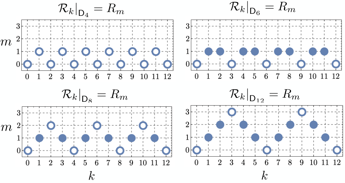
Restriction from to acts on irreps in the following way:
| (13a) | ||||
| (13b) | ||||
where we have introduced the function
| (14) |
and defined the (reducible) representations
| (15a) | ||||
| (15b) | ||||
A.0.2 Tensor representations
The orthogonal group has a natural action on real-valued, -dimensional, rank- tensors of the form , given by
| (16) |
which may be thought of as “rotating each index as a vector.” We will be working exclusively in two dimensions, and so we define as the vector space of real -dimensional, rank- tensors. It is clear then that acts 16 on via the representation , which will reduce into a direct sum of irreducible -representations according to the decomposition rules given in Eq. 9.
Consider the vector space of rank-2 tensors. Tensors of this type are especially relevant for viscometry, since the strain tensor is an element of this space. Eq. 9 then tells us that the action 16 of on is reducible:
| (17) |
An explicit basis of that achieves this block diagonalization is
| (18) |
where, if is understood to mean that the vector lies in the subspace transforming exclusively under the representation , we have that
| (19a) | ||||
| (19b) | ||||
| (19c) | ||||
Illustrated explicitly for a given , we see that
| (20) | ||||
which is nothing other than the familiar statement that rank-2 tensors decompose into a trace, an antisymmetric, and a traceless symmetric “part” (i.e. projection into an irreducible subspace), with this decomposition preserved under rotations and reflections.
Let us now restrict from the action 17 of on to the action of on . Then we see from the branching rules 13 that and hence
| (27) |
The reduction of to two -dimensional irreducible representations upon restriction to is precisely the mechanism responsible for the splitting of shear viscosity when rotational symmetry of the Fermi surface is broken in favor of square symmetry. This can be seen by the fact that the two viscosity tensor terms and pick out rate of strain tensors that live in this symmetry sector. Similarly, the decomposition 27 tells us that there will generically be viscosity tensor terms that pick out fluid motion living in the and irreducible representations: these are precisely the bulk viscosity and rotational viscosity , respectively.
Finally, consider the rank-4 tensor space , of which the viscosity tensor is an element. Eq. 9 then tells us that the action 16 on is reducible as
| (28) |
An explicit basis of that achieves this block diagonalization is given by
| (29) |
In Eq. 29, we have omitted indices, with their placement implied by the order of tensors; the indices go on the first (left) tensor in any product, and the indices on the second (right) tensor. For example, . We have also further diagonalized equivalent irreps according to their parity under time reversal (, or equivalently in the above notation, switching the order of tensors in any product), with extra hats being put on irreps that are time-reversal odd.
To say that a viscosity tensor is isotropic, i.e. -invariant, is simply the statement that , i.e. it transforms trivially under the action 16. From the basis 29, we can already see the generality of the isotropic () viscosity tensor 1 from the main text; only the terms that belong to the trivial representation may appear in the isotropic viscosity tensor 1. For the isotropic tensor 1, we have excluded the tensor despite it belonging to the trivial representation , simply because the corresponding component is proportional to the antisymmetric part of a stress tensor , which much always vanish by angular momentum conservation in an isotropic theory.
If we relax our notion of isotropy and no longer demand invariance under reflection, then tensors belonging to the representation may also be included, i.e. the first six tensors in Eq. 29. These six tensors exactly match those found in recent work [48] enumerating the most general viscosity tensors allowed in an “isotropic” (allowing for non-trivial reflection parity) fluid. Furthermore, the tensors given in Eq. 29 also contain those found in recent work [46] on Hall viscosities in anisotropic fluids with broken time-reversal symmetry.
Upon restriction from to , we see from the branching rules 13 that none of the non-trivial basis elements (not lying in the irrep ) 29 become trivial, i.e. we get no new invariant tensors upon restriction to . However, in this case, anisotropy allows the stress tensor to have an antisymmetric component , and so we now include the invariant tensor in Eq. 1.
Upon restriction from to , the irrep decomposes and contains a trivial irrep, since per Eq. 13. This means that we may now use the first basis element in the subspace 29 in our -invariant viscosity tensor. This vector , when taken into linear combinations with the always-trivial vector , then allows the tensors and to appear independently in the viscosity tensor 1. This is again the origin of the shear viscosity splitting upon restriction to .
See Table 2 for a visualization of the five irreps realized as boundary conditions on our dihedral viscometer. By enforcing current boundary conditions with symmetry of a selected irrep, one may restrict dissipation at the square center to selected dissipative coefficients (e.g. viscosity components discussed above) as desired.
Finally, similar considerations for the restriction of to give the following symmetry-allowed viscosity tensor in fluids:
| (30) | ||||
Taken in addition to Eq. 1, Section A.0.2 completes the specification of the most general viscosity tensor allowed in dihedral fluids of any degree M. In Section A.0.2, we have used hats to indicate the viscosities which are time-reversal odd; these viscosities will only appear in fluids which, in addition to their low rotational symmetry, have also broken time-reversal symmetry.
Appendix B Comparison of our viscometry and channel flow techniques
In this section, we compare our viscometry technique to those based on flow profiles in long channels, a more conventional probe of electronic viscosity. In long, one-dimensional channels with no-slip boundary conditions at the walls, viscous flow leads to a parabolic (Poiseuille) velocity profile [1]. The curvature of this parabolic velocity profile is set by (a component of) the fluid viscosity, with larger viscosities giving rise to smaller curvature and vice-versa; by measuring this velocity profile curvature (or the integrated flow it induces), the relevant viscosity component may be inferred.
As it is the most general possible case, we consider the hydrodynamic flow of a -invariant fluid A.0.2, forced by an applied field (i.e. pressure gradient) through an infinite 1D channel of transverse width . Channel flows of -invariant Dirac fluids (e.g. charge neutral graphene) were studied in [26], in which a viscometry procedure was also proposed. Their proposal involved measuring the curvature of the resulting Poiseuille channel profile, as a function of the relative angle between the channel and fluid’s symmetry/crystallographic axes. The suggested procedure then exploits this angular freedom to (in principle) extract multiple viscosity components of the fluid.
We assume that the channel coordinates are rotated
by an angle relative to the fluid coordinates . As described above, the fluid is forced through the channel by an electric field of strength , applied in the positive -direction. Assuming no-slip at the channel walls , the static velocity profile is then the parabolic, Poiseulle solution [1]
| (37) |
where is the relevant channel viscosity component, properly rotated from the fluid coordinates via Eq. 16; using Eqs. 16 and A.0.2, this component is computed to be
| (38) |
or, equivalently, in Cartesian coordinates of the fluid:
| (39) |
Our approach possesses several manifest advantages over such rotated channel flow experiments.
Firstly, as can be seen from both Eq. 38 and Eq. 39, such rotated Poiseuille flows can distinguish at most unique viscosity components, of the total A.0.2 allowed in fluids ( total if time-reversal is a symmetry). By contrast, we expect the boundary condition irreps in (i.e. ) to give distinct heat measurements at the center of a square/rectangle viscometer, from which (linear combinations of) of the viscosity components A.0.2 may be inferred. Moreover, for higher symmetry cases (to which our approach naturally generalizes), it is clear that our viscometry will continue to distinguish strictly more viscosities than rotated channels (e.g. in fluids).
Secondly, even in fluids of exceptionally-low symmetry, for which irreducible boundary conditions are not enough to uniquely isolate all viscosities, our viscometry nevertheless continues to group viscosities according to their symmetry class. For example, boundary currents on a square sample of fluid would lead to center heating from , , (and thus be unable to distinguish them) — but those alone, and none of the other allowed in . As a caveat: in order to use our framework to measure viscosities in a -invariant fluid, one will need to compare experimental heating measurements with e.g. detailed hydrodynamic simulations.
Thirdly, the feasibility of such rotated-channel experiments relies on the ability to cut the requisite channel samples at various angles relative to the crystal axes. In order to distinguish even the channel viscosities 38 just discussed, different channel angles must be used, therefore requiring at least one mesoscopic sample misaligned with the crystallographic axes. By contrast, our viscometry relies not on the geometry of the boundary, but rather its symmetry. For example, for the fluids discussed in the main text, square samples/boundaries are not required; isolated centered heating will still be guaranteed even with circular samples/boundaries, so long as the current boundary conditions remain -irreducible.
Appendix C Kinetic theory
In this appendix, we discuss the extent to which our argument in the main text generalizes to account for ballistic effects. For a sufficiently weakly interacting electron fluid, we can solve Boltzmann equations to calculate transport coefficients beyond the hydrodynamic regime [52]. As in the main text, we study time-independent flows within linear response. Letting denote the deviation of the distribution function of kinetic theory away from equilibrium, the form of the kinetic equations is schematically:
| (40) |
where denotes the microscopic (single-particle) group velocity arising from the single-particle dispersion relation, and denotes the linearized collision integral. We have also introduced Dirac notation to emphasize that the function is to be regarded as an infinite-dimensional vector in momentum space, so that
| (41) |
We assume, as usual, that the collision integral is local in space.
Without specifying any microscopic details, what can we say on the basis of symmetry alone? As in the main text, let us imagine solving this Boltzmann equation 40 in a region , which admits a natural group action by a symmetry group , by which we mean the spatial geometry and the dispersion relation are -invariant. Now suppose the spatial geometry contains a point which is fixed by the action of , i.e. for all . Consider a solution of the Boltzmann equation 40, evaluated at this fixed point. Then the action of on the vector space of fixed-point-evaluated distributions , given by
| (42) |
restricts to only the momentum-dependence.
Since is assumed to be a group of symmetries, we know that the linearized collision integral 41 is invariant under the group action 42. But then Schur’s lemma [38] tells us that the vector space of possible fixed point momentum distributions ’s may be written as a direct sum of -irreducible subspaces , each acted upon by the action 42 of according to an irrep of , so that acts proportionally to the identity on each irreducible subspace . This allows us to write
| (43) |
where denotes a projector onto , and are the proportionality constants. We have introduced the extra label to account for the inevitable appearance of multiple copies of each irrep ; it is entirely analogous to the quantum number that appears in the wave functions of a rotationally-invariant quantum mechanical model, where only indices specify the rotational symmetry.
Note that, by the decomposition 43, the irreducible subspaces are also eigenspaces of the linearized collision integral , with the corresponding eigenvalues playing the same role mathematically as the viscosity components described in the main text. In the context of kinetic theory, the collision integral eigenvalues have the physical interpretation as scattering rates associated with various scattering mechanisms/pathways.
If we now choose boundary conditions which transform exclusively under a given irrep of the symmetry group , then the function , as the solution of a -invariant differential equation 40 with -covariant boundary conditions, must also transform according to the irrep under the group action 42. In other words, . This result then allows us to express the vector as
| (44) |
where for each .
The fixed point heating is then calculated in kinetic theory as
| (45) |
Importantly, the scattering rates that contribute to the fixed point heat 45 are isolated to only those in Eq. 43 for which , the irrep specified by the boundary conditions. We therefore conclude: only dissipative mechanisms that couple to momentum functions belonging to the same irrep as the boundary conditions contribute to heat at a fixed point . In the hydrodynamic regime, these dissipative mechanisms are viscosities (to leading order in the small parameter , with the characteristic length scale of ). The fixed point heat 45 is analogous to the selected isolation of a single term in the heating decomposition 5 given in the main text (though in that case, there are no repeated irreps, so there is no index).
Finally, we address a subtlety that arises when we instead allow the boundary condition symmetry group to be a subgroup of the fluid symmetry group , in which case we must slightly generalize Eq. 45. For concreteness, let us now take boundary conditions which transform under a given irrep of . When the irreps of are restricted to , they generate representations of , which are in general reducible with respect to . So in this case, fixed point heating can be generated by all irreps of for which the irreducible decomposition of contains , the boundary condition irrep of . Put another way, the smaller symmetry group of the device determines the constrained heating, not the larger fluid symmetry group .
As a result, if an isotropic fluid is placed in a viscometer with boundary conditions, irreducible with respect to a dihedral subgroup such as , then there will be extremely small heating at a fixed point in the hydrodynamic regime. The leading contribution to heat generated at the center of the device comes from kinetic theory modes that are in the representation of , since the decomposition contains . In the hydrodynamic regime, one finds that in a device of size , with electron-electron scattering length , [53]
| (46a) | ||||
| (46b) | ||||
where is the total current that enters/exits through one of the contacts 11 1 The scaling follows from dimensional analysis, as is (up to overall prefactors that are not relevant here) the integral over the one-dimensional boundary of velocity.. We therefore conclude that (in the limit , so that dimensional analysis can be trusted) the total fixed point heating obeys
| (47) |
In a Fermi liquid where , the heating is extremely small; the and dependence of is extreme and remains a diagnostic for the absence of rotational viscosity in such a system. After all, the rotational heating (in the hydrodynamic regime) instead scales as
| (48) |
which is easily distinguishable.
Boundary conditions with full symmetry correspond to the Taylor-Couette device geometry, i.e. constant, perfectly tangential velocity everywhere along a circular/cylindrical boundary. Even though these boundary conditions satisfy and therefore set all perturbative ballistic corrections 47 to zero at the fixed point (i.e. the center of the circular geometry), they are physically unrealizable in an electronic system, for which only orthogonal currents can be readily controlled.
Appendix D Estimating temperature signal due to viscous heating
In this appendix, we give an order of magnitude estimate for the expected temperature variation to be measured at the center of the dihedral viscometer, described in the main text and reported in Fig. 2. In doing so, we consult recent experimental data for hydrodynamic electrons in doped monolayer graphene [6, 7]; these works report the following parameter values appropriate for the onset of hydrodynamic behavior in monolayer graphene:
| (49a) | ||||
| (49b) | ||||
| (49c) | ||||
| (49d) | ||||
| (49e) | ||||
where is the electron density, the electron temperature, the Gurzhi length, the kinematic (shear) viscosity, and the DC electrical conductivity.
We begin by estimating the electronic thermal conductivity , which can – within an order of magnitude, in current experimental devices – be related to the electrical conductivity via the Wiedemann-Franz relation
| (50) |
Solving for and substituting in monolayer graphene paramter values, we estimate
| (51) |
We will also require the shear viscosity , where is the quasiparticle mass. In monolayer graphene we may estimate by equating the linear and cyclotronic momenta, with Fermi wavevector in two dimensions and typical Fermi velocity [1] in monolayer graphene. Altogether, this gives a shear viscosity
| (52) |
As anisotropic viscosity components (such as ) have never been measured in experiment, we will further assume that all viscosity components are approximately equal to the above shear viscosity in graphene. For anisotropic electron hydrodynamics in ABA trilayer graphene, this assumption is justified by recent theoretical calculations in a microscropic model [55].
Finally, we apply dimensional analysis to restore units to the center heats , and hence the center temperature variations 6, numerically obtained from the dimensionless biharmonic equation 3 given in the main text. The magnitude of strain rates appearing in the sample will depend on choice of experimental parameters (the size of the viscometer) and (the currents applied to the sample); we take
| (53a) | ||||
| (53b) | ||||
where is chosen so that ohmic effects do not dominate the onset of hydrodynamics, and is a current value typical for linear response experiments in such systems. Letting represent the dimensionless center strain rates obtained from Eq. 3, we find
Signals of this magnitude are easily detectable using existing local thermometry based on nitrogen-vacancy centers in diamond: see e.g. [41].
Appendix E Advantages for experiments
In this appendix, we present additional figures that summarize nice properties of our proposed viscometer for an experiment. In Fig. 5 we demonstrate that the determination of anisotropy is not substantially modified by momentum-relaxing scattering. In Fig. 6, we further demonstrate that the center heat signal is extremely robust to nonzero momentum relaxation, within a typical hydrodynamic regime . Even toward the ohmic limit at still stronger momentum-relaxation, only the rotational center heating is significantly affected. Fig. 7 demonstrates a method to uniquely determine using only four total center heat measurements. Fig. 8 shows how the electric potentials and electric fields are expected to look for various configurations of the dihedral viscometer.


Appendix F Flow plots
In this appendix, we collect some useful plots that demonstrate flow patterns in our proposed viscometer, including how they change as a function of parameters. Fig. 9 shows the and flow patterns that we did not show in the main text. Fig. 10 shows a diversity of flow patterns in the configuration; Fig. 11 in the configuration; and Fig. 12 in the configuration. Fig. 13 shows how the rotational viscosity signal disappears as a function of as the center vortex switches orientation; Fig. 14 shows the formation of 4 vortices at the center of the viscometer in the configuration.