A Damped Newton algorithm for Generated Jacobian Equations

Anatole Gallouët Address: Univ. Grenoble Alpes, CNRS, Grenoble INP, LJK, 38000 Grenoble, France Email address: anatole.gallouet@univ-grenoble-alpes.fr , Quentin Mérigot Address: Université Paris-Saclay, CNRS, Laboratoire de mathématiques d’Orsay, 91405, Orsay, France and Institut universitaire de France (IUF) Email address: quentin.merigot@universite-paris-saclay.fr and Boris Thibert Address: Univ. Grenoble Alpes, CNRS, Grenoble INP, LJK, 38000 Grenoble, France Email address: Boris.Thibert@univ-grenoble-alpes.fr

Date: August 11, 2026

Abstract.

Generated Jacobian Equations have been introduced by Trudinger [Disc. cont. dyn. sys (2014), pp. 1663–1681] as a generalization of Monge-Ampère equations arising in optimal transport. In this paper, we introduce and study a damped Newton algorithm for solving these equations in the semi-discrete setting, meaning that one of the two measures involved in the problem is finitely supported and the other one is absolutely continuous. We also present a numerical application of this algorithm to the near-field parallel refractor problem arising in non-imaging problems.

1. Introduction

This paper is concerned with the numerical resolution of Generated Jacobian equations, introduced by N. Trudinger [19] as a generalization of Monge-Ampère equations arising in optimal transport. Generated Jacobian equations were originally motivated by inverse problems arising in non-imaging optics in the near-field case [12, 7, 8] but they also apply to problems arising in economy [16, 5]. A survey on these equations and their applications was recently written by N. Guillen [6]. The input for a generated Jacobian equations are two probability measures $\mu$ and $\nu$ over two spaces $X$ and $Y$ , and a generating function $G:X\times Y\times\mathbb{R}\to\mathbb{R}$ . Loosely speaking, a scalar function $\psi$ on $Y$ is an Alexandrov solution to the generated jacobian equation if the map $T_{\psi}$ defined by

T_{\psi}(x)\in\argmax_{y\in Y}G(x,y,\psi(y))

transports $\mu$ onto $\nu$ , i.e. $\nu$ is the image of the measure $\mu$ under $T_{\psi}$ , denoted

T_{\psi\#}\mu=\nu.

Note that one needs to impose some conditions on $\mu$ and $G$ ensuring that the map $T_{\psi}$ is well-defined $\mu$ -almost everywhere. One can describe the meaning of this equation using an economic metaphor. We consider $X$ as a set of customers, $Y$ as a set of products and $G(x,y,\psi(y))$ corresponds to the utility of the product $y$ for the customer $x$ given a price $\psi(y)$ . The probability measure $\mu$ and $\nu$ describe the distribution of customers and products. The map $T_{\psi}$ can be described as the “best response” of customers given a price menu $\psi:Y\to\mathbb{R}$ : each customer $x\in X$ tries to maximize its own utility $G(x,y,\psi(y))$ over all products $y\in Y$ : the maximizer, if it exists and is unique, is denoted $T_{\psi}(x)$ . Then, $\psi$ is a solution to the generated jacobian equation if the best response map $T_{\psi}$ pushes the distribution of customers to the distribution of available products $\nu$ .

In this article, we are interested in algorithms for solving the semi-discrete case, where the source measure $\mu$ is absolutely continuous with respect to the Lebesgue measure on $X\subseteq\mathbb{R}^{d}$ and the target measure $\nu$ is finitely supported. Such discretization can be traced back to Minkowski, but have been used more recently to solve Monge-Ampère equations [17], problems from non-imaging optics [4], more general optimal transport problems [10], but also generated Jacobian equations [1]. In all the cited papers, the methods are coordinate-wise algorithms with minimal increment and are similar to the algorithm introduced by Oliker-Prussner [17]. The number of iterations of these algorithms scales more than cubicly ( $N^{3}$ , where $N$ is the size of the support of $\nu$ ), making them limited to fairly small discretizations. More recently, Newton methods have been introduced to solve semi-discrete optimal transport problems [11, 14]. In this paper, we show that newtonian techniques can also be applied to Generated Jacobian equations under mild conditions on the generating function $G$ .

Semi-discrete optimal transport.

The semi-discrete setting refers to the case where one is given an absolutely continuous probability measure $\mu$ (with respect to the Lebesgues measure) supported on a domain $X$ of $\mathbb{R}^{d}$ and a discrete probability measure $\nu=\sum_{y}\nu_{y}\delta_{y}$ supported on a finite set $Y$ . Given a cost function $c:X\times Y\to\mathbb{R}$ , the optimal transport problem amounts to finding a function $T:X\to Y$ that minimizes the total cost $\int_{X}c(x,T(x))d\mu(x)$ under the condition $\mu(T^{-1}(y))=\nu_{y}$ for any $y\in Y$ . This problem can be recast, using Kantorovitch duality under some mild conditions on the cost $c$ , into finding a dual potential $\psi:Y\to\mathbb{R}$ that satisfies

\forall y\in Y\quad\mu(\mathrm{Lag}_{y}(\psi))=\nu_{y}\

(

\mathrm{MA}

)

where $\mathrm{Lag}_{y}(\psi)$ are the Laguerre cells defined by

\mathrm{Lag}_{y}(\psi)=\left\{x\in X\mid\forall z\in Y,c(x,y)+\psi(y)\leq c(x,z)+\psi(z)\right\}.

The application $T_{\psi}$ defined for $x\in X$ by $T_{\psi}(x)=y$ if $x\in\mathrm{Lag}_{y}(\psi)$ is then an optimal transport map between $\mu$ and $\nu$ for the cost $c$ , and satisfies in particular $T_{\psi\#}\mu=\nu$ . Equation ( MA ) can be regarded as a discrete version of the Monge-Ampère type equation arising in optimal transport. We refer for instance to [2, §2] for more details in the case $c(x,y)=-\langle x|y\rangle$ .

Generated Jacobian equation.

The Generated Jacobian equation in the semi-discrete setting has a very similar form. The problem also amounts to finding a function $\psi:Y\to\mathbb{R}$ that satisfies Equation ( MA ), but the Laguerre cells have a more general form and read

\mathrm{Lag}_{y}(\psi)=\left\{x\in X\mid\forall z\in Y,G(x,y,\psi(y))\geq G(x,z,\psi(z))\right\}

where $G$ is called a generating function. When $G$ is linear in the last variable, i.e. when $G(x,y,v)=-c(x,y)-v$ , one obviously recovers the Laguerre cells from optimal transport.

Note that the lack of linearity in the generating function $G$ adds several theoretical and practical difficulties. To see this, consider the mass function

\displaystyle H:\mathbb{R}^{Y}\to\mathbb{R}^{Y},~~\psi\mapsto(\mu(\mathrm{Lag}_{y}(\psi)))_{y\in Y}.

In the optimal transport case, the function $H$ is invariant under the addition of a constant (i.e. $H(\psi+c)=H(\psi)$ for any $c\in\mathbb{R}$ ), which entails under mild assumptions that the kernel of $\mathrm{D}H(\psi)$ has rank one and coincides with the vector space of constant functions on $Y$ [11]. Furthermore, as a consequence of Kantorovitch duality, the function $H$ is the gradient of a functional, called Kantorovitch functional in [11]. This implies that the differential $\mathrm{D}H(\psi)$ is symmetric. In the case of generated Jacobian equations, these two properties do not hold anymore: the differential $\mathrm{D}H(\psi)$ is not necessarily symmetric and its kernel is not reduced to the set of constant functions in general.

In this article, we generalize the damped Newton algorithm proposed in [11] to solve generated Jacobian equations. Note that unlike [11] we do not require any Ma-Trudinger-Wang type condition to prove the convergence of our algorithm. In Section 2 we recall the notion of generating function and its properties, and introduce the generated Jacobian equation in the semi-discrete setting. Section 3 is entirely dedicated to the numerical resolution of the generated Jacobian equation. In Section 4, we apply our algorithm to numerically solve the Near Field Parallel Reflector problem. Note that F. Abedin and C. Gutierrez also consider this problem [1], but their algorithm requires a strong condition, called Visibility Condition, that implies the Twist condition (defined hereafter) of the generating function $G$ . We show that under a much weaker assumption, this twist condition holds for a subset of dual potential $\psi:Y\to\mathbb{R}$ on which we can apply our algorithm. It is very likely that our assumption could also be adapted to [1].

2. Semi-discrete generated Jacobian equation

In this section, we recall the notions introduced by N. Trudinger in order to define the generated Jacobian equation [19] in the semi-discrete setting. Let $\Omega$ be an open bounded domain of $\mathbb{R}^{d}$ , let $X$ be a compact subset of $\Omega$ and let $Y$ be a finite set of $\mathbb{R}^{d}$ . Let $\mu$ be a measure on $\Omega$ , which is absolutely continuous with respect to the Lebesgue measure, with non-negative density $\rho$ supported on $X$ (i.e. $\supp(\rho)\subset X$ ), and let $\nu=\sum_{y\in Y}\nu_{y}\delta_{y}$ be a measure on the finite set $Y$ such that all $\nu_{y}$ are positive ( $\nu_{y}>0$ ). These two measures must satisfy the mass balance condition $\mu(X)=\nu(Y)$ and it is not restrictive to view them as probability measures:

\int_{X}\rho(x)dx=\sum_{y\in Y}\nu_{y}=1

Notations. We denote by $\mathcal{H}^{k}$ the $k$ -dimensional Hausdorff measure in $\mathbb{R}^{d}$ . In particular $\mathcal{H}^{d}$ is the Lebesgue measure in $\mathbb{R}^{d}$ . The set of functions from $Y$ to $\mathbb{R}$ is denoted by $\mathbb{R}^{Y}$ . We denote by $\langle\cdot|\cdot\rangle$ the Euclidean scalar product, by $\|\cdot\|$ the Euclidean norm, by $\mathrm{B}(x,r)$ the Euclidean ball of center $x$ and radius $r$ , by $\chi_{A}:\mathbb{R}^{d}\to\{0,1\}$ the indicator function of a set $A$ . The image and kernel of a matrix $M$ are respectively denoted by $\im(M)$ and $\ker(M)$ . We denote by $\Span(u)$ the linear space spanned by a vector $u$ , by $\nabla_{x}G$ the gradient of a function $G$ with respect to $x$ and by $\partial_{v}G$ its scalar derivative with respect to $v$ . Finally, for $N\in\mathbb{N}$ , we denote $\llbracket 1,N\rrbracket=\{1,\ldots,N\}$ .

2.1. Generating function

We recall below the notion of generating function and $G$ -convexity in the semi-discrete setting [19, 1].

Definition 1 (Generating function).

Let $a,b\in\mathbb{R}\cup\{-\infty,+\infty\}$ with $a<b$ and $I=]a,b[$ . A function $G:\Omega\times Y\times I\to\mathbb{R}$ is called a generating function. We assume that it satisfies the following properties:

•

Regularity condition: $(x,y,v)\mapsto G(x,y,v)$ is continuously differentiable in $x$ and $v$ , and

$\forall\alpha<\beta\in I,\sup_{(x,y,v)\in\Omega\times Y\times[\alpha,\beta]}|\nabla_{x}G(x,y,v)|<+\infty$
•

Monotonicity condition:

$\forall(x,y,v)\in\Omega\times Y\times I:\partial_{v}G(x,y,v)<0$
•

Twist condition:

$\forall x\in\Omega,(y,v)\mapsto(G(x,y,v),\nabla_{x}G(x,y,v))\text{ is injective on }Y\times I$
•

Uniform Convergence condition:

$\forall y\in Y,\lim_{v\to a}\inf_{x\in\Omega}G(x,y,v)=+\infty$

Remark 2 (Range of $G$ ).

Through the whole paper we can and will consider that $I=\mathbb{R}$ . Indeed suppose that $G:\Omega\times Y\times I\to\mathbb{R}$ satisfies the assumptions of the above definition. Considering a strictly increasing $\mathcal{C}^{1}$ diffeomorphism $\zeta:\mathbb{R}\to I$ and setting $\widetilde{G}(x,y,v)=G(x,y,\zeta(v))$ , we get a generating function $\tilde{G}:\Omega\times Y\times\mathbb{R}\to\mathbb{R}$ , which also satisfies the conditions above. Moreover, up to reparametrization, the generated Jacobian equations associated to $G$ and $\tilde{G}$ are equivalent.

Remark 3.

Note that F. Abedin and C. Gutierrez [1] impose a slightly more restrictive inequality in condition (• ‣ 1): their supremum is taken over $\Omega\times Y\times]-\infty,\alpha]$ for any $\alpha$ instead of $\Omega\times Y\times[\alpha,\beta]$ . We changed here this condition in order to handle the Near Field point reflector problem in the last section.

Definition 4 (G-convexity).

Let $\varphi:\Omega\to\mathbb{R}$ be a function. If $\varphi\geq G(\cdot,y_{0},\lambda_{0})$ for all $x\in\Omega$ with equality at $x=x_{0}$ , we say that the function $G(\cdot,y_{0},\lambda_{0})$ supports $\varphi$ at $x_{0}$ . A function $\varphi:\Omega\to\mathbb{R}$ is said to be G-convex if it is supported at every point, i.e. for all $x_{0}\in\Omega$ ,

\exists(y_{0},\lambda_{0})\in Y\times\mathbb{R}\text{ s.t. }\begin{cases}\forall x\in\Omega,\varphi(x)\geq G(x,y_{0},\lambda_{0})\\ \varphi(x_{0})=G(x_{0},y_{0},\lambda_{0})\end{cases}

(2.1)

Remark 5 (Relation with convexity).

The notion of G-convexity generalizes in a certain sense the notion of convexity. Intuitively, it amounts to replacing the supporting hyperplanes by functions of the form $G(\cdot,y,\lambda)$ . If $G(\cdot,y,\lambda)$ is convex for any $y\in Y$ and any $\lambda\in\mathbb{R}$ , then a $G$ -convex function is always convex. Moreover, if the generating function $G$ is affine (i.e $G(x,y,\lambda)=\langle x,y\rangle+\lambda$ ) and if $Y=\mathbb{R}^{d}$ , then the notions of G-convexity and convexity are equivalent.

Definition 6 (G-subdifferential).

Let $\varphi$ be a G-convex function and let $x_{0}\in\Omega$ . The G-subdifferential $\partial_{G}\varphi$ of $\varphi$ at $x_{0}$ is defined by

\partial_{G}\varphi(x_{0})=\left\{y\in Y\mid\exists\lambda_{0}\in\mathbb{R}\text{s.t. $G(\cdot,y,\lambda_{0})$ supports $\varphi$ at $x_{0}$}\right\}

(2.2)

The following lemma (Lemma 2.1 in [1]) shows that the $\partial_{G}\varphi$ is single-valued almost everywhere, and induces a measurable

Lemma 7.

[1, Lemma 2.1] Let $\varphi$ be G-convex with $G$ satisfying (• ‣ 1), (• ‣ 1) and (• ‣ 1). Then, there exists a measurable map $S_{\varphi}:\Omega\to Y$ s.t.

\hbox{ for a.e. }x\in\Omega,\quad\partial_{G}\varphi(x)=\{S_{\varphi}(x)\}.

We can define the notion of generated Jacobian equation.

Definition 8 (Brenier solution to the GJE).

A function $\varphi:X\to\mathbb{R}$ is a Brenier solution to the generated Jacobian equation between a probability density $\mu$ on $\Omega$ and a probability measure $\nu=\sum_{y\in Y}\nu_{y}\delta_{y}$ on $Y$ if it satisfies

\begin{cases}\varphi\text{ is G-convex}\\ \forall y\in Y,\mu(S_{\varphi}^{-1}(\{y\}))=\nu_{y}\end{cases}

(GenJac)

2.2. G-transform

The goal in this section is to write a dual formulation of the generated Jacobian equation, using the notion of $G$ -transform introduced by Trudinger [19].

Definition 9.

The $G$ -transform $\psi^{G}:\Omega\to\mathbb{R}$ of $\psi:Y\to\mathbb{R}$ is defined by

\forall x\in\Omega,~~\psi^{G}(x)=\max_{y\in Y}G(x,y,\psi(y)).

(2.3)

Proposition 10.

Assume $G$ satisfies (• ‣ 1), (• ‣ 1) and (• ‣ 1) and let $\varphi:\Omega\to\mathbb{R}$ be a $G$ -convex function. Then there exists $\psi:S_{\varphi}(\Omega)\to\mathbb{R}$ s.t.

\forall x\in\Omega,~~\varphi(x)=\max_{y\in S_{\varphi}(\Omega)}G(x,y,\psi(y))

Proof.

Let $y\in S_{\varphi}(\Omega)$ , then for any $x_{0}\in S_{\varphi}^{-1}(y)$ there exists $\lambda_{0}\in\mathbb{R}$ such that $\varphi(x_{0})=G(x_{0},y,\lambda_{0})$ . Since $\varphi$ is $G$ -convex we also have for any $x\in\Omega$ that $\varphi(x)\geq G(x,y,\lambda_{0})$ . Specifically for $x_{1}\in S_{\varphi}^{-1}(y)$ , we get $\varphi(x_{1})=G(x_{1},y,\lambda_{1})\geq G(x_{1},y,\lambda_{0})$ and since $\partial_{v}G(x,y,v)<0$ then $\lambda_{1}\leq\lambda_{0}$ . By symmetry we have $\lambda_{1}=\lambda_{0}$ . We can deduce that there exists a unique $\psi(y)\in\mathbb{R}$ such that for any $x\in S_{\varphi}^{-1}(y),\varphi(x)=G(x,y,\psi(y))$ . This defines a map $\psi:S_{\varphi}(\Omega)\to\mathbb{R}$ satisfying

\forall x\in\Omega,~\begin{cases}\forall y\in S_{\varphi}(\Omega),\varphi(x)\geq G(x,y,\psi(y))\\ \exists y\in S_{\varphi}(\Omega),\varphi(x)=G(x,y,\psi(y))\end{cases}

As a conclusion we have $\displaystyle\varphi(x)=\max_{y\in S_{\varphi}(\Omega)}G(x,y,\psi(y))$ . ∎

Corollary 11.

Let $\varphi$ be a $G$ -convex function such that $S_{\varphi}(\Omega)=Y$ , then there exists $\psi:Y\to\mathbb{R}$ such that $\varphi=\psi^{G}$ .

Remark 12 ( $G$ -convex functions are not always $G$ -transforms).

Without any additional assumptions on the generating function, we cannot guarantee that any $G$ -convex function $\varphi$ on $X$ is the $G$ -transform of a function $\psi$ on $Y$ . Define for instance

\Omega=(1,2),\quad Y=\{0,1\},\quad G(x,y,v)=\begin{cases}xe^{-v}&\hbox{ if }y=0\\ -xv&\hbox{ if }y=1\end{cases}.

and consider the function $\varphi$ on $\Omega$ defined by $\varphi(x)=G(x,1,1)=-x$ , which is $G$ -convex by definition. Yet for any $v\in\mathbb{R}$ and any $x\in\Omega$ ,

\max(G(x,0,v),G(x,1,1))=\max(xe^{-v},-x)=xe^{-v},

thus implying that that there does not exist any $\psi:Y\to\mathbb{R}$ such that $\varphi$ is the $G$ -transform of $\psi$ .

Suppose that $\varphi$ is a solution of (GenJac) and that for all $y\in Y$ , the mass $\nu_{y}$ is positive. Then, for any $y\in Y$ one has $\mu(S_{\varphi}^{-1}(y))=\nu_{y}>0$ , which guarantees that $S_{\varphi}(\Omega)=Y$ . Therefore by Corollary 11 there exists a function $\psi$ on $Y$ such that $\varphi=\psi^{G}$ . This means that we can reparametrize the problem (GenJac) by assuming that the solution $\varphi$ is the $G$ -transform of some function $\psi$ . The sets $S_{\psi^{G}}^{-1}(\{y\})$ , which appear in (GenJac) will be called generalized Laguerre cells.

Definition 13 (Generalized Laguerre cells).

The generalized Laguerre cells associated to a function $\psi:Y\to\mathbb{R}$ are defined for every $y\in Y$ by

	$\displaystyle\mathrm{Lag}_{y}(\psi)$	$\displaystyle:=S_{\psi^{G}}^{-1}(\{y\})$		(2.4)
		$\displaystyle=\left\{x\in\Omega\mid\forall z\in Y,G(x,y,\psi(y))\geq G(x,z,\psi(z))\right\}.$		(2.4)

Note that by Lemma 7, the intersection of two generalized Laguerre cells has zero Lebesgue measure, ensuring that the sets $\mathrm{Lag}_{y}(\psi)$ form a partition of $\Omega$ up to a $\mu$ -negligible set.

Definition 14 (Alexandrov solution to GJE).

A function $\psi:Y\to\mathbb{R}$ is an Alexandrov solution to the generated Jacobian equation between generated Jacobian equation between a probability density $\mu$ on $\Omega$ and a probability measure $\nu=\sum_{y\in Y}\nu_{y}\delta_{y}$ on $Y$ if $\psi^{G}$ is a Brenier solution (Definition 8) to the same GJE, or equalently if

\forall y\in Y,~~H_{y}(\psi)=\nu_{y},\quad\hbox{ where }H_{y}(\psi)=\mu(\mathrm{Lag}_{y}(\psi)).

Setting $H(\psi)=(H_{y}(\psi))_{y\in Y}$ and considering $\nu$ as a function over $Y$ , we can even rewrite this equation as

H(\psi)=\nu.

(GenJacD)

3. Resolution of the generated Jacobian equation

The goal of this section is to introduce and study a Newton algorithm to solve the semi discrete generated Jacobian equation (GenJacD). Before doing so, we study the regularity of the mass function $H:\mathbb{R}^{Y}\to\mathbb{R}^{Y}$ in Section 3.1 and establish a non-degeneracy property of its differential $\mathrm{D}H$ in Section 3.2, under a connectedness assumption on the support of the source measure. We present the algorithm and prove its convergence in Section 3.3.

For simplicity, we will number the points in $Y$ , i.e. we assume that

Y=\{y_{1},\ldots,y_{N}\},

where the points $y_{i}$ are distinct. This allows us to identify the set of functions $\mathbb{R}^{Y}$ with $\mathbb{R}^{N}$ , by setting $\psi_{i}=\psi(y_{i})$ . We also denote $(e_{i})_{1\leq i\leq N}$ the canonical basis of $\mathbb{R}^{N}$ . Finally, we introduce a shortened notation for Laguerre cells and intersections thereof

\mathrm{Lag}_{i}(\psi)=\mathrm{Lag}_{y_{i}}(\psi),\quad\mathrm{Lag}_{ij}(\psi)=\mathrm{Lag}_{i}(\psi)\cap\mathrm{Lag}_{j}(\psi).

Throughout this section, we assume that the generating function $G$ satisfies all the conditions of Definition 1.

3.1. $\mathcal{C}^{1}$ -regularity of $H$

The differentiability of $H$ is established under a (mild) genericity hypothesis on the cost function, ensuring in particular that the intersection between three distinct Laguerre cells is negligible with respect to the $(d-1)$ -dimensional Hausdorff measure, denoted $\mathcal{H}^{d-1}$ . To write this hypothesis, we denote for three distinct indices $i,j,k$ in $\llbracket 1,N\rrbracket$ ,

\Gamma_{ij}(\psi)=\{x\in\Omega\mid G(x,y_{i},\psi_{i})=G(x,y_{j},\psi_{j})\},\quad\Gamma_{ijk}(\psi)=\Gamma_{ij}(\psi)\cap\Gamma_{ik}(\psi).

Definition 15 (Genericity of the generating function.).

The generating function $G$ is generic with respect to $\Omega$ and $Y$ if for any distinct indices $i,j,k$ in $\llbracket 1,N\rrbracket$ and any $\psi\in\mathbb{R}^{N}$ we have

\mathcal{H}^{d-1}(\Gamma_{ijk}(\psi))=0.

(

\mathrm{Gen}_{\Omega}^{Y}

)

The generating function $G$ is generic with respect to the boundary $\partial X$ and $Y$ if for any distinct indices $i,j$ in $\llbracket 1,N\rrbracket$ and any $\psi\in\mathbb{R}^{N}$ we have

\mathcal{H}^{d-1}(\Gamma_{ij}(\psi)\cap\partial X)=0.

(

\mathrm{Gen}_{\partial X}^{Y}

)

Proposition 16.

Assume that

•

$G\in\mathcal{C}^{2}(\Omega\times Y\times\mathbb{R})$ satisfies (• ‣ 1), (• ‣ 1), (• ‣ 1), ( Gen Ω Y ), ( Gen ∂ X Y ),
•

$X\subseteq\Omega$ is compact and that $\rho$ is a continuous probability density on $X$ .

Then the mass function $H:\mathbb{R}^{N}\to\mathbb{R}^{N}$ defined by $H(\psi)=(\mu(\mathrm{Lag}_{i}(\psi)))_{1\leq i\leq N}$ has class $\mathcal{C}^{1}$ . We have for $\psi\in\mathbb{R}^{N}$ and $i\in\llbracket 1,N\rrbracket$

\begin{cases}\displaystyle\frac{\partial H_{j}}{\partial\psi_{i}}(\psi)=\int_{\mathrm{Lag}_{ij}(\psi)}\rho(x)\frac{|\partial_{v}G(x,y_{i},\psi_{i})|}{\|\nabla_{x}G(x,y_{j},\psi_{j})-\nabla_{x}G(x,y_{i},\psi_{i})\|}d\mathcal{H}^{d-1}(x)\geq 0\text{ for }j\neq i\\ \displaystyle\frac{\partial H_{i}}{\partial\psi_{i}}(\psi)=-\sum_{j\neq i}\frac{\partial H_{j}}{\partial\psi_{i}}(\psi)\end{cases}

(3.5)

Proof.

Let $\psi\in\mathbb{R}^{N}$ and $i,j\in\llbracket 1,N\rrbracket$ be fixed indices such that $i\neq j$ . We want to compute $\partial H_{j}/\partial\psi_{i}(\psi)$ . For this purpose, we introduce $\psi^{t}=\psi+te_{i}$ for $t\geq 0$ . From (• ‣ 1), we obviously have $\mathrm{Lag}_{j}(\psi)\subseteq\mathrm{Lag}_{j}(\psi^{t})$ . Therefore

H_{j}(\psi^{t})-H_{j}(\psi)=\mu(\mathrm{Lag}_{j}(\psi^{t}))-\mu(\mathrm{Lag}_{j}(\psi))=\mu(\mathrm{Lag}_{j}(\psi^{t})\setminus\mathrm{Lag}_{j}(\psi))

We introduce the set $L$ obtained by removing one inequality in the definition of the generalized Laguerre cell $\mathrm{Lag}_{j}(\psi)$ :

L=\{x\in\Omega\mid\forall k\neq i,G(x,y_{j},\psi_{j})\geq G(x,y_{k},\psi_{k})\}.

We have in particular $\mathrm{Lag}_{j}(\psi)\subseteq L$ and more precisely

\mathrm{Lag}_{j}(\psi^{t})\setminus\mathrm{Lag}_{j}(\psi)=\bigsqcup_{0<s\leq t}L\cap\Gamma_{ij}(\psi^{t}).

We will use this formula to get another expression of $H_{j}(\psi^{t})-H_{j}(\psi)$ .

Step 1. Construction of $u_{ij}$ such that $\Gamma_{ij}(\psi^{t})=u_{ij}^{-1}(\{t\})$ . To construct such a function $u_{ij}:\Omega\to\mathbb{R}$ , we first consider the function $f_{ij}:\Omega\times\mathbb{R}\to\mathbb{R}$ defined by

f_{ij}(x,t)=G(x,y_{j},\psi_{j})-G(x,y_{i},\psi_{i}+t)

This function $f_{ij}$ is of class $\mathcal{C}^{1}$ on $\Omega\times\mathbb{R}$ by hypothesis on $G$ and we have

\forall(x,t)\in\Omega\times\mathbb{R},\frac{\partial f_{ij}}{\partial t}(x,t)=-\partial_{v}G(x,y_{i},\psi_{i}+t)>0.

This implies that a fixed $x\in\Omega$ , the function $f_{ij}(x,\cdot)$ is strictly increasing, so that equation $f_{ij}(x,t)=0$ has at most one solution. Denoting

\mathcal{V}_{ij}=\{x\in\Omega\mid\exists t\in\mathbb{R},f_{ij}(x,t)=0\}=\bigcup_{t\in\mathbb{R}}\Gamma_{ij}(\psi^{t}),

one can therefore define a function $u_{ij}:\mathcal{V}_{ij}\to\mathbb{R}$ which satisfies

\forall x\in\mathcal{V}_{ij},~~f_{ij}(x,t)=0\Longleftrightarrow u_{ij}(x)=t.

By the implicit function theorem, the set $\mathcal{V}_{ij}$ is open and the function $u_{ij}$ is $\mathcal{C}^{1}$ on $\mathcal{V}_{ij}$ . In order to apply the co-area formula, we need to compute the gradient of $u_{ij}$ . For any point $x$ in $\mathcal{V}_{ij}$ , we have by definition

f_{ij}(x,u_{ij}(x))=G(x,y_{j},\psi_{j})-G(x,y_{i},\psi_{i}+u_{ij}(x))=0.

Differentiating this expression with respect to $x$ , we obtain

\nabla u_{ij}(x)=\frac{\nabla_{x}G(x,y_{j},\psi_{j})-\nabla_{x}G(x,y_{i},\psi_{i}+u_{ij}(x))}{\partial_{v}G(x,y_{i},\psi_{i}+u_{ij}(x))}

which is well defined since $\partial_{v}G(x,y_{i},v)<0$ on $\Omega\times Y\times\mathbb{R}$ by the (• ‣ 1) hypothesis. The (• ‣ 1) condition guarantees that for all $x\in\mathcal{V}_{ij}$ , the map $(y,v)\mapsto(G(x,y,v),\nabla_{x}G(x,y,v))$ is injective. By definition of $u_{ij}$ we have $f_{ij}(x,u_{ij}(x))$ , so that

G(x,y_{j},\psi_{j})=G(x,y_{i},\psi_{i}+u_{ij}(x)).

The (• ‣ 1) condition then entails

\nabla_{x}G(x,y_{j},\psi_{j})\neq\nabla_{x}G(x,y_{i},\psi_{i}+u_{ij}(x)),

implying that the gradient $\nabla u_{ij}(x)$ does not vanish.

Step 2. Computation of the partial derivatives. We can write the difference between Laguerre cells using the function $u_{ij}$ :

	$\displaystyle\mathrm{Lag}_{j}(\psi^{t})\setminus\mathrm{Lag}_{j}(\psi)$	$\displaystyle=\bigcup_{0<s\leq t}\mathrm{Lag}_{ij}(\psi^{s})$
		$\displaystyle=\left\{x\in\Omega,\exists s\in]0,t],f_{ij}(x,s)=0\right\}\cap L$
		$\displaystyle=\left\{x\in\Omega,\exists s\in]0,t],u_{ij}(x)=s\right\}\cap L$
		$\displaystyle=u_{ij}^{-1}(]0,t])\cap L,$

giving directly

H_{j}(\psi^{t})-H_{j}(\psi)=\mu(L\cap u_{ij}^{-1}(]0,t]))=\int_{L\cap u_{ij}^{-1}(]0,t])}\rho(x)dx.

Then the co-area formula gives us

\frac{H_{j}(\psi^{t})-H_{j}(\psi)}{t}=\frac{1}{t}\int_{L\cap u_{ij}^{-1}(]0,t])}\rho(x)dx=\frac{1}{t}\int_{0}^{t}H_{ij}(\psi^{s})ds,

where we introduced

\displaystyle H_{ij}(\psi)=\int_{\mathrm{Lag}_{ij}(\psi)}\frac{\rho(x)}{\|\nabla u_{ij}(x)\|}d\mathcal{H}^{d-1}(x).

(3.6)

Note that thanks to the computations above, we already know that the gradient $\nabla u_{ij}(x)$ does not vanish. Moreover, for any $x$ in $\mathrm{Lag}_{ij}(\psi)\subseteq\Gamma_{ij}(\psi)$ , one has $u_{ij}(x)=0$ . Thus,

\nabla u_{ij}(x)=(\nabla_{x}G(x,y_{j},\psi_{j})-\nabla_{x}G(x,y_{i},\psi_{i}))/(\partial_{v}G(x,y_{i},\psi_{i})).

We can therefore rewrite

\displaystyle H_{ij}(\psi)=\int_{\mathrm{Lag}_{ij}(\psi)}\frac{\rho(x)|\partial_{v}G(x,y_{i},\psi_{i})|}{|\nabla_{x}G(x,y_{j},\psi_{j})-\nabla_{x}G(x,y_{i},\psi_{i})|}d\mathcal{H}^{d-1}(x).

(3.7)

As shown in Proposition 17 below, $H_{ij}$ is continuous on $\mathbb{R}^{N}$ . We deduce that

\frac{\partial H_{j}}{\partial\psi_{i}}(\psi)=\lim_{t\to 0,t>0}\frac{H_{j}(\psi^{t})-H_{j}(\psi)}{t}=H_{ij}(\psi)\geq 0.

(3.8)

The case $t<0$ can be treated similarly by replacing $\mathrm{Lag}_{j}(\psi)\subseteq\mathrm{Lag}_{j}(\psi^{t})$ with $\mathrm{Lag}_{j}(\psi^{t})\subseteq\mathrm{Lag}_{j}(\psi)$ . We thus get the desired expression for the partial derivative $\partial H_{j}/\partial\psi_{i}$ for $i\neq j$ .

To compute the partial derivative for $j=i$ , we use the mass conservation property $\sum_{1\leq i\leq N}H_{i}(\psi)=1$ to deduce that

\frac{\partial H_{i}}{\partial\psi_{i}}(\psi)=-\sum_{j\neq i}\frac{\partial H_{j}}{\partial\psi_{i}}(\psi).\qed

It remains to show that the functions $H_{ij}$ used in the proof of Proposition 16 are continuous.

Proposition 17.

Under the assumptions of Proposition 16, for every $i,j\in\llbracket 1,N\rrbracket$ , the function $H_{ij}$ defined in (3.6) is continuous on $\mathbb{R}^{N}$ .

Proof.

We introduce the function $g:\Omega\times\mathbb{R}^{N}\to\mathbb{R}$ defined by

g(x,\psi)=\bar{\rho}(x)\frac{|\partial_{v}G(x,y_{i},\psi_{i})|}{\|\nabla_{x}G(x,y_{j},\psi_{j})-\nabla_{x}G(x,y_{i},\psi_{i})\|}

where $\bar{\rho}$ is a continuous extension of the probability density $\rho_{|X}$ on $\Omega$ . For a given $\psi\in\mathbb{R}^{N}$ , the (• ‣ 1) hypothesis guarantees that for any $x\in\Gamma_{ij}(\psi)$ , $\nabla_{x}G(x,y_{j},\psi_{j})\neq\nabla_{x}G(x,y_{i},\psi_{i})$ . This implies that $g$ is continuous on a neighborhood of the set $\{(x,\psi)\in\Omega\times\mathbb{R}^{N}|x\in\Gamma_{ij}(\psi)\}$ . We introduced in Proposition 16 the function

H_{ij}(\psi)=\int_{\mathrm{Lag}_{ij}(\psi)\cap X}g(x,\psi)d\mathcal{H}^{d-1}(x).

Let $\psi^{\infty}\in\mathbb{R}^{N}$ and $\psi^{n}$ a sequence converging towards $\psi^{\infty}$ .The main difficulty for proving that $H_{ij}(\psi^{n})$ converges to $H_{ij}(\psi^{\infty})$ as $n\to+\infty$ is that the integrals in the definition of $H_{ij}(\psi^{n})$ and $H_{ij}(\psi^{\infty})$ are over different hypersurfaces, namely $\Gamma_{ij}(\psi^{n})$ and $\Gamma_{ij}(\psi^{\infty})$ . Our first step will therefore be to construct a diffeomorphism between (subsets) of these hypersurfaces. We introduce $f:\mathbb{R}\times\mathbb{R}\times\Omega\to\mathbb{R}$ the function defined by

f(a,b,x)=G(x,y_{j},\psi^{\infty}_{j}+a)-G(x,y_{i},\psi^{\infty}_{i}+b)

We put $a_{n}=\psi_{j}^{n}-\psi_{j}^{\infty}$ and $b_{n}=\psi_{i}^{n}-\psi_{i}^{\infty}$ , so that $a_{n}\to 0$ and $b_{n}\to 0$ as $n$ tends to $+\infty$ . We also have

\Gamma_{ij}(\psi^{\infty})=(f(0,0,\cdot))^{-1}(0),\quad\Gamma_{ij}(\psi^{n})=(f(a_{n},b_{n},\cdot))^{-1}(0).

Step 1: Construction of a map $F_{n}$ between $\Gamma_{ij}(\psi^{\infty})$ and $\Gamma_{ij}(\psi^{n})$ .
This map is constructed using the composition of the flows associated to two vector fields $X_{a}$ and $X_{b}$ . Let $\widetilde{\Omega}\subset\Omega$ an open domain containing $X$ . The (• ‣ 1) hypothesis guarantees that there exists a neighborhood $\widetilde{V}$ of the set $\{(a,b,x)\in\mathbb{R}^{2}\times\widetilde{\Omega}| f(a,b,x)=0 \}$ such that we have for any $v\in\widetilde{V}$ , $\nabla_{x}f(v)\neq 0$ . We can then define two vector fields $X_{a},X_{b}$ on $\widetilde{V}$ by

	$\displaystyle X_{a}(a,b,x)$	$\displaystyle=\left(1,0,-\partial_{a}f(a,b,x)\frac{\nabla_{x}f(a,b,x)}{\\|\nabla_{x}f(a,b,x)\\|^{2}}\right)$
	$\displaystyle X_{b}(a,b,x)$	$\displaystyle=\left(0,1,-\partial_{b}f(a,b,x)\frac{\nabla_{x}f(a,b,x)}{\\|\nabla_{x}f(a,b,x)\\|^{2}}\right)$

Since $f$ is of class $\mathcal{C}^{2}$ , $X_{a}$ and $X_{b}$ are both of class $\mathcal{C}^{1}$ on $\widetilde{V}$ . We then consider $\Phi_{a}$ and $\Phi_{b}$ the flows associated respectively to $X_{a}$ and $X_{b}$ defined for $(t,v)\in[-\varepsilon,\varepsilon]^{2}\times\widetilde{V}$ by

\begin{cases}\Phi_{a}(0,v)=v\\ \partial_{t}\Phi_{a}(t,v)=X_{a}(\Phi(t,v))\end{cases}

and

\begin{cases}\Phi_{b}(0,v)=v\\ \partial_{t}\Phi_{b}(t,v)=X_{b}(\Phi(t,v))\end{cases}

The vector fields $X_{a}$ and $X_{b}$ are continuously differentiable on $\widetilde{V}$ which implies that both $\Phi_{a}(t,\cdot)$ and $\Phi_{b}(t,\cdot)$ converge pointwise in the $\mathcal{C}^{1}$ sense toward the identity as $t\to 0$ . Let $(t,v)\in[-\varepsilon,\varepsilon]\times\widetilde{V}$ . Denoting $\nabla f(v)=(\partial_{a}f,\partial_{b}f,\nabla_{x}f)(v)$ , we then have

	$\displaystyle f(\Phi_{a}(t,v))$	$\displaystyle=f(\Phi_{a}(0,v))+\int_{0}^{t}\frac{\partial}{\partial s}\big(s\mapsto f(\Phi_{a}(s,v))\big)ds$
		$\displaystyle=f(v)+\int_{0}^{t}\langle\nabla f(\Phi_{a}(s,v))\|\partial_{t} \Phi_{a}(s,v)\rangle ds$
		$\displaystyle=f(v)+\int_{0}^{t}\langle\nabla f(\Phi_{a}(s,v))\|X_{a}(\Phi_{a}(s,v))\rangle ds$
		$\displaystyle=f(v)$

Similarly one has $f(\Phi_{b}(t,v))=f(v)$ . Let $\Pi:\widetilde{V}\to\Omega$ the projection of $\widetilde{V}\subseteq\mathbb{R}^{2}\times\Omega$ on $\Omega$ , and let $F_{n}:\Gamma_{ij}(\psi^{\infty})\cap\widetilde{\Omega}\to\Omega$ be the function defined by

F_{n}(x)=\Pi\big(\Phi_{a}(a_{n},\Phi_{b}(b_{n},(0,0,x)))\big).

For $x\in\Gamma_{ij}(\psi^{\infty})$ and $v=(0,0,x)\in\widetilde{V}$ , we have

\Phi_{a}(a_{n},\Phi_{b}(b_{n},v))=(a_{n},b_{n},F_{n}(x))

and from the previous equality we deduce that

f(\Phi_{a}(a_{n},\Phi_{b}(b_{n},v)))=f(v)=0

This means that for $x\in\Gamma_{ij}(\psi^{\infty})$ , $F_{n}(x)\in\Gamma_{ij}(\psi^{n})$ . Moreover $\Phi_{a}(a_{n},\cdot)$ and $\Phi_{b}(b_{n},\cdot)$ are both invertible of inverse $\Phi_{a}(-a_{n},\cdot)$ and $\Phi_{b}(-b_{n},\cdot)$ . Thus $F_{n}$ is also invertible of inverse

F_{n}^{-1}(x)=\Pi\big(\Phi_{b}(-b_{n},\Phi_{a}(-a_{n},(a_{n},b_{n},x)))\big)

Since both $\Phi_{a}(a_{n},\cdot)$ and $\Phi_{b}(b_{n},\cdot)$ converge pointwise in the $\mathcal{C}^{1}$ toward the identity as $n\to+\infty$ , we have for $x\in\Gamma_{ij}(\psi^{\infty})\cap\widetilde{\Omega}$

\begin{cases}\displaystyle\lim_{n\to+\infty}F_{n}(x)=x,\\ \displaystyle\lim_{n\to+\infty}JF_{n}(x)=1,\end{cases}

where $JF_{n}$ is the absolute value of the determinant of the Jacobian matrix of $F_{n}$ .

Step 2: Convergence of $H_{ij}(\psi^{n})$ toward $H_{ij}(\psi^{\infty})$ .
We let $L_{\infty}=\mathrm{Lag}_{ij}(\psi^{\infty})$ and $L_{n}=F_{n}^{-1}(\mathrm{Lag}_{ij}(\psi^{n})\cap\widetilde{\Omega})$ . Denoting by $\chi_{A}$ the indicator function of a set $A$ , we have

	$\displaystyle H_{ij}(\psi^{\infty})$	$\displaystyle=\int_{\Gamma_{ij}(\psi^{\infty})}g(x,\psi^{\infty})\chi_{X}(x)\chi_{L_{\infty}}(x)d\mathcal{H}^{d-1}(x)$
		$\displaystyle=\int_{\Gamma_{ij}(\psi^{\infty})\cap\widetilde{\Omega}}g(x,\psi^{\infty})\chi_{X}(x)\chi_{L_{\infty}}(x)d\mathcal{H}^{d-1}(x)$

because $\Gamma_{ij}(\psi^{\infty})\cap X\subset\widetilde{\Omega}$ . We also have

H_{ij}(\psi^{n})=\int_{\Gamma_{ij}(\psi^{n})}g(x,\psi^{n})\chi_{X}(x)\chi_{\mathrm{Lag}_{ij}(\psi^{n})}(x)d\mathcal{H}^{d-1}(x)

By a change of variable from $x$ to $F_{n}(x)$ , the latter equality becomes

H_{ij}(\psi^{n})=\int_{\Gamma_{ij}(\psi^{\infty})\cap\widetilde{\Omega}}g(F_{n}(x),\psi^{n})JF_{n}(x)\chi_{X}(F_{n}(x))\chi_{L_{n}}(x)d\mathcal{H}^{d-1}(x)

where $JF_{n}(x)$ denotes the determinant of the Jacobian matrix of $F_{n}$ . We already have the pointwise convergences $F_{n}(x)\to x$ and $JF_{n}(x)\to 1$ as $n\to\infty$ . If we can show that

\lim_{n\to+\infty} \chi_{X}(F_{n}(x))\chi_{L_{n}}(x)=\chi_{X}(x)\chi_{L_{\infty}}(x)

for $\mathcal{H}^{d-1}$ almost every point $x$ , then using Lebesgue’s dominated convergence theorem, we will obtain that $H_{ij}(\psi^{n})\to H_{ij}(\psi^{\infty})$ .

We first show that $\lim_{n\to+\infty}\chi_{L_{n}}(x)\to\chi_{L_{\infty}}(x)$ $\mathcal{H}^{d-1}$ -almost everywhere on $\Gamma_{ij}(\psi^{\infty})\cap\widetilde{\Omega}$ . We first consider the superior limit: given $x\in\Gamma_{ij}(\psi^{\infty})\cap\widetilde{\Omega}$ , we prove that $\limsup_{n\to\infty}\chi_{L_{n}}(x)\leq\chi_{L_{\infty}}(x)$ . The limsup is non-zero if and only if there exists a subsequence $(\sigma(n))_{n\in\mathbb{N}}$ such that $\forall n\in\mathbb{N},x\in L_{\sigma(n)}$ . In this case we have $F_{\sigma(n)}(x)\in F_{\sigma(n)}(L_{\sigma(n)})=\mathrm{Lag}_{ij}(\psi^{\sigma(n)})\cap\widetilde{\Omega}$ . This means that for any $k\neq i,j$

G(F_{\sigma(n)}(x),y_{i},\psi_{i}^{\sigma(n)})=G(F_{\sigma(n)}(x),y_{j},\psi_{j}^{\sigma(n)})\leq G(x,y_{k},\psi_{k}^{\sigma(n)})

Since $G$ is continuous the previous inequality passes to the limit $n\to\infty$ , showing that $x\in L_{\infty}$ , and that

\limsup_{n\to\infty}\chi_{L_{n}}(x)\leq\chi_{L_{\infty}}(x)

We now want to show $\liminf_{n\to\infty}\chi_{L_{n}}(x)\geq\chi_{L_{\infty}}(x)$ . If $x\notin L_{\infty}$ the result is straightforward. Let us consider the set

S_{ij}=\left(\bigcup_{k\neq i,j}\Gamma_{ijk}(\psi^{\infty})\right)\cup(\Gamma_{ij}(\psi^{\infty})\cap\partial X)

(3.9)

By the genericity hypothesis (Definition 15) we have $\mathcal{H}^{d-1}(S_{ij})=0$ . If $x\in L_{\infty}\setminus S_{ij}$ , by definition we get for every $k\not\in\{i,j\}$ that $x$ does not belong to $\Gamma_{jk}(\psi^{\infty})$ . This implies a strict inequality

G(x,y_{i},\psi_{i}^{\infty})=G(x,y_{j},\psi_{j}^{\infty})<G(x,y_{k},\psi_{k}^{\infty}).

Since $F_{n}(x)$ converges to $x$ and since $\psi^{n}$ converges to $\psi^{\infty}$ , we get for $n$ large enough

\begin{cases}G(F_{n}(x),y_{i},\psi_{i}^{n})<G(F_{n}(x),y_{k},\psi_{k}^{n})\\ G(F_{n}(x),y_{j},\psi_{j}^{n})<G(F_{n}(x),y_{k},\psi_{k}^{n}).\end{cases}

Moreover since $x\in\Gamma_{ij}(\psi^{\infty})$ , $F_{n}(x)\in\Gamma_{ij}(\psi^{n})$ . Combining the inequalities above, this shows that $F_{n}(x)$ belongs to $\mathrm{Lag}_{ij}(\psi^{n})\cap\widetilde{\Omega}=F_{n}(L_{n})$ , i.e. $x\in L_{n}$ . This gives us

\forall x\not\in S_{ij},\quad\liminf_{n\to\infty}\chi_{L_{n}}(x)\geq\chi_{L_{\infty}}(x).

Consider $x\not\in S_{ij}$ . For such $x$ , we already know that $\chi_{L_{n}}(x)\to\chi_{L_{\infty}}(x)$ as $n\to+\infty$ . Thus, if $x$ does not belong to $L_{\infty}$ , we directly have

\lim_{n\to+\infty}\chi_{L_{n}}(x)\chi_{X}(F_{n}(x))=\chi_{L_{\infty}}\chi_{X}(x)=0.

We may now assume that $x$ belongs to $L_{\infty}\setminus S_{ij}$ . By definition of $S_{ij}$ , this implies that $x\notin\partial X$ . We can directly deduce that $\chi_{X}$ is continuous at $x$ and that $\chi_{X}(F_{n}(x))\to\chi_{X}(x)$ when $n\to+\infty$ .

In conclusion we have that $H_{ij}(\psi^{n})\to H_{ij}(\psi^{\infty})$ , so that $H_{ij}$ is continuous. ∎

3.2. Kernel and image of $\mathrm{D}H$

The goal of this section is to prove Proposition 18 that gives properties on the differential of the mass function $H$ . We consider the admissible set

\mathcal{S}^{+}=\left\{\psi\in\mathbb{R}^{N}\mid\forall i\in\llbracket 1,N\rrbracket,H_{i}(\psi)>0\right\}.

(3.10)

Proposition 18.

In addition to the assumptions of Proposition 16, we assume that

\inter(X)\cap\{\rho>0\}\hbox{ is path-connected },

where $\inter(X)$ is the interior of $X$ . Then we have for any $\psi\in\mathcal{S}^{+}$

•

The differential $DH(\psi)$ has rank $N-1$ ;
•

The image of $DH$ is $\im(DH(\psi))=\mathrm{\textbf{1}}^{\perp}$ where $\mathrm{\textbf{1}}=(1,\cdots,1)\in\mathbb{R}^{N}$ ;
•

For any $w\in\ker(DH(\psi))\setminus\{0\}$ , we have for all $i\in\llbracket 1,N\rrbracket,w_{i}\neq 0$ and all $w_{i}$ have the same sign.

The next two lemmas have already been included in the recent survey on optimal transport involving the second and third authors [15], but we include them here for completeness. The proof of Proposition 18 is different from the previous work in optimal transport because $H$ is not symmetric.

Lemma 19.

Let $U\subset\mathbb{R}^{d}$ be a path-connected open set, and $S\subset\mathbb{R}^{d}$ be a closed set such that $\mathcal{H}^{d-1}(S)=0$ . Then, $U\setminus S$ is path-connected.

Proof.

It suffices to treat the case where $U$ is an open ball, the general case will follow by standard connectedness arguments. Let $x,y\in U\setminus S$ be distinct points. Since $U\setminus S$ is open, there exists $r>0$ such that $\mathrm{B}(x,r)$ and $\mathrm{B}(y,r)$ are included in $U\setminus S$ . Consider the hyperplane $H$ orthogonal to the segment $[x,y]$ , and $\Pi_{H}$ the projection on $H$ . Then, since $\Pi_{H}$ is 1-Lipschitz, $\mathcal{H}^{d-1}(\Pi_{H}S)\leq\mathcal{H}^{d-1}(S)=0$ , so that $H\setminus\Pi_{H}S$ is dense in the hyperplane $H$ . In particular, there exists a point $z\in\Pi_{H}(\mathrm{B}(x,r))\setminus S=\Pi_{H}(\mathrm{B}(y,r))\setminus S$ . By construction the line $z+\mathbb{R}(y-x)$ avoids $S$ and passes through the balls $\mathrm{B}(x,r)\subset U\setminus S$ and $\mathrm{B}(y,r)\subset U\setminus S$ . This shows that the points $x,y$ can be connected in $U\setminus S$ . ∎

We define for $\psi\in\mathbb{R}^{N}$ the graph $\mathcal{G}_{\psi}=(V,E)$ with vertex set $V=\{1,\ldots,N\}$ with edges

E=\left\{(i,j)\in V^{2}\mid\frac{\partial H_{i}}{\partial\psi_{j}}(\psi)>0\right\}

We have the following result.

Lemma 20.

Under the assumptions of Proposition 18 and for $\psi\in\mathcal{S}^{+}$ , the graph $\mathcal{G}_{\psi}$ is connected.

Proof.

Let $Z=\inter(X)\cap\{\rho>0\}$ , and $S=\bigcup_{ij}S_{ij}$ where $S_{ij}$ is defined in (3.9). From Lemma 19 the set $Z\setminus S$ is path connected, we also have $\mu(Z\setminus S)=1$ since $\mu(\partial X)=\mu(S)=0$ . Suppose that $\mathcal{G}_{\psi}$ is not connected. Let $i_{0}\in\llbracket 1,N\rrbracket$ , and let $I_{0}$ be the connected component of $i_{0}$ in the graph $\mathcal{G}_{\psi}$ . We thus have $i_{0}\in I_{0}\neq\llbracket 1,N\rrbracket$ . We consider the two non-empty sets

U_{1}=\bigcup_{i\in I_{0}}\mathrm{Lag}_{i}(\psi)\cap(Z\setminus S)\text{ and }U_{2}=\bigcup_{i\notin I_{0}}\mathrm{Lag}_{i}(\psi)\cap(Z\setminus S),

which partition $Z\setminus S$ up to a Lebesgue-negligible set. Moreover, since $\psi\in\mathcal{S}^{+},$

\begin{cases}U_{1}\cup U_{2}=Z\setminus S,\\ 0<\mu(U_{1})<1,\\ 0<\mu(U_{2})<1.\end{cases}

By construction $U_{1}$ and $U_{2}$ are closed sets in $Z\setminus S$ . Since $\mu(U_{i})>0$ we can pick $x$ and $y$ in $Z\setminus S$ such that $x\in U_{1}$ and $y\in U_{2}$ . The $Z\setminus S$ being path-connected, we know that there exists a path $\gamma\in\mathcal{C}^{0}([0,1],Z\setminus S)$ satisfying $\gamma(0)=x$ and $\gamma(1)=y$ . We let $t=\max\{s\in[0,1]|\gamma(s)\in U_{1}\}$ and we are going to show that $\gamma(t)\in U_{1}\cap U_{2}$ . By construction, $\gamma(t)$ obviously belongs to $U_{1}$ . Now if $t=1$ we have $\gamma(t)=y\in U_{2}$ . If not, we have for all $\epsilon>0$ that $\gamma(t+\epsilon)\in U_{2}$ . Since $U_{2}$ is relatively closed in $Z\setminus$ and since $\gamma$ is continuous, we have $\gamma(t)\in U_{2}$ . Naming $z=\gamma(t)$ , there exists $i\in I_{0}$ , $j\notin I_{0}$ such that $z\in\mathrm{Lag}_{i}(\psi)\cap\mathrm{Lag}_{j}(\psi)$ . Moreover, since $z\notin S$ we get that for any $k\notin\{i,j\}$ ,

G(z,y_{i},\psi_{i})=G(z,y_{j},\psi_{j})>G(z,y_{k},\psi_{k}).

By continuity of $G$ we can deduce that there exists an open ball of radius $r>0$ such that

\forall x\in\mathrm{B}(z,r),\forall k\notin\{i,j\},G(x,y_{i},\psi_{i})>G(x,y_{k},\psi_{k})

This implies that

\mathrm{B}(z,r)\cap\Gamma_{ij}(\psi)\subset\mathrm{Lag}_{ij}(\psi)

where $\Gamma_{ij}(\psi)$ is defined in Definition 15. By (• ‣ 1) condition and the inversion function theorem, we know that $\Gamma_{ij}(\psi)$ is a $d-1$ dimensional manifold and $z\in\Gamma_{ij}(\psi)$ . Moreover we have $\rho(z)>0$ because $z\in Z$ and $\rho$ is continuous on $Z\subset X$ by hypothesis. We now have

	$\displaystyle\frac{\partial H_{i}}{\partial\psi_{j}}(\psi)$	$\displaystyle=\int_{\mathrm{Lag}_{ij}(\psi)}\rho(x)\frac{\|\partial_{v}G(x,y_{i},\psi_{i})\|}{\\|\nabla_{x}G(x,y_{j},\psi_{j})-\nabla_{x}G(x,y_{i},\psi_{i})\\|}d\mathcal{H}^{d-1}(x)$
		$\displaystyle\geq\int_{\mathrm{B}(z,r)\cap\Gamma_{ij}(\psi)}\rho(x)\frac{\|\partial_{v}G(x,y_{i},\psi_{i})\|}{\\|\nabla_{x}G(x,y_{j},\psi_{j})-\nabla_{x}G(x,y_{i},\psi_{i})\\|}d\mathcal{H}^{d-1}(x)>0$

which is a contradiction with the hypothesis that $i$ and $j$ are not connected in the graph $\mathcal{G}_{\psi}$ . ∎

Proof of Proposition 18.

We note the matrix $M=DH(\psi)$ , with coefficients $m_{i,j}=\partial H_{i}/\partial\psi_{j}(\psi)$ . We first show that $\ker(M^{T})=\Span(\mathrm{\textbf{1}})$ . The inclusion $\mathrm{\textbf{1}}\in\ker(M^{T})$ follows from

\sum_{i=1}^{N}m_{i,j}=\frac{\partial}{\partial\psi_{j}}\left(\sum_{i=1}^{N}H_{i}(\psi)\right)=0.

Consider now $v\in\ker(M^{T})$ , and pick an index $i_{0}$ where $v$ is maximum, i.e. $i_{0}\in\argmax_{1\leq i\leq N}v_{i}$ . We have

0=(M^{T}v)_{i_{0}}=\sum_{i=1}^{N}m_{i,i_{0}}v_{i}=\sum_{i\neq i_{0}}m_{i,i_{0}}v_{i}+m_{i_{0},i_{0}}v_{i_{0}}=\sum_{i\neq i_{0}}m_{i,i_{0}}(v_{i}-v_{i_{0}}).

Since $\psi\in\mathcal{S}^{+}$ , we have by Proposition 16 that for $i\neq i_{0}$ , $m_{i,i_{0}}\geq 0$ . By definition of $i_{0}$ we also have $v_{i}-v_{i_{0}}\leq 0$ . From all this we deduce that $v_{i}=v_{i_{0}}$ for any $i\neq i_{0}$ satisfying $m_{i,i_{0}}>0$ , i.e. any vertex $i$ adjacent to $i_{0}$ in the graph $\mathcal{G}_{\psi}$ . By connectedness of $\mathcal{G}_{\psi}$ , we conclude that $v=v_{i_{0}}\mathrm{\textbf{1}}$ , thus showing $\ker(M^{T})=\Span(\mathrm{\textbf{1}})$ .

We can deduce from this result that $M$ is of rank $N-1$ because $\rk(M)=\rk(M^{T})=N-1$ . Moreover for any $u\in\mathbb{R}^{N}$ ,

\langle\mathrm{\textbf{1}},Mu\rangle=(Mu)^{T}\mathrm{\textbf{1}}=u^{T}M^{T}\mathrm{\textbf{1}}=0.

Since the spaces $\im(M)$ and $\mathrm{\textbf{1}}^{\perp}$ have the same dimension, we immediately get $\im(M)=\mathrm{\textbf{1}}^{\perp}$ .

Let $w\in\ker(M)\setminus\{0\}$ , we now want to show that for all $i\in\llbracket 1,N\rrbracket,w_{i}\neq 0$ and that all of the $w_{i}$ have the same sign. The proof consists in two steps:

•

Step 1: we show that $w\geq 0$ (or $-w\geq 0$ ).
•

Step 2: we show that for $i\in\llbracket 1,N\rrbracket$ , $w_{i}>0$ .

We define $\lambda=\max_{i}|m_{i,i}|$ and $A=\lambda I+M$ . With these definitions, $v$ belongs to $\ker(M)$ if and only if $Av=\lambda v$ . Moreover, for any $i,j\in\llbracket 1,N\rrbracket$ , one has $a_{i,j}\geq 0$ and

\displaystyle\sum_{k=1}^{N}a_{k,j}=\lambda.

Step 1: Assume that there exists $i_{0}\in\llbracket 1,N\rrbracket$ such that $w_{i_{0}}\geq 0$ (we can do this without loss on generality, by working on $-w$ otherwise). Suppose that there exists $j\neq i_{0}$ such that $a_{i_{0},j}>0$ and $w_{j}<0$ , then since $Aw=\lambda w$ , we have $\lambda w_{i_{0}}=\sum_{j=1}^{N}a_{i_{0},j}w_{j}$ and thus $\lambda|w_{i_{0}}|<\sum_{j=1}^{N}a_{i,j}|w_{j}|$ . We also have for any $i\in\llbracket 1,N\rrbracket,\lambda|w_{i}|\leq\sum_{j=1}^{N}a_{i,j}|w_{j}|$ . By summing this inequality on $i$ and since the inequality is strict when $i=i_{0}$ , we obtain

\sum_{i=1}^{N}\lambda|w_{i}|<\sum_{i=1}^{N}\sum_{j=1}^{N}a_{i,j}|w_{j}|=\sum_{j=1}^{N}|w_{j}|\sum_{i=1}^{N}a_{i,j}=\sum_{j=1}^{N}\lambda|w_{j}|,

which is a contradiction, so we can affirm that there exists no index $j\neq i_{0}$ such that $w_{j}<0$ and $a_{i_{0},j}>0$ . Since $A=M+\lambda I$ , for $j\neq i_{0},a_{i_{0},j}=m_{i_{0},j}$ . We thus have $\forall j\in\llbracket 1,N\rrbracket,m_{i_{0},j}>0\implies w_{j}\geq 0$ . By connectedness of $\mathcal{G}$ we deduce $w\geq 0$ .

Step 2: If there exists $i\in\llbracket 1,N\rrbracket$ such that $w_{i}=0$ , then $\sum_{j}a_{i,j}w_{j}=0$ . Recall that by construction $a_{i,j}\geq 0$ and with step 1 $w_{j}\geq 0$ , so we have $\forall j,a_{i,j}>0\implies w_{j}=0$ . Again by connectedness of $\mathcal{G}$ we have $w=0$ .

∎

Remark 21.

Remark that a part of the proof of Proposition 18 could also be seen as a consequence of the Perron Frobenius theorem, using the notions of irreducible and stochastic matrices. The matrix $A=M+\lambda I$ can be written $A=\lambda S$ where $S^{T}$ is a stochastic matrix. The matrix $S$ is thus of spectral radius $1$ and $A$ is of spectral radius $\lambda$ . Since $M$ is irreducible, $A$ is also irreducible. Perron Frobenius Theorem then implies that $\lambda$ is a simple eigenvalue with an associated eigenvector $w$ satisfying $w_{i}>0$ for any $i\in\llbracket 1,N\rrbracket$ . Since $Av=\lambda v\iff Mv=0$ , we can deduce that $\rk(M)=N-1$ and $\ker(M)=\Span(w)$ . Moreover since $\mathrm{\textbf{1}}\in\ker(M^{T})$ , we have for any $u\in\mathbb{R}^{N}$ , $\langle\mathrm{\textbf{1}},Mu\rangle=(Mu)^{T}\mathrm{\textbf{1}}=u^{T}M^{T}\mathrm{\textbf{1}}=0$ and $\im(M)=\mathrm{\textbf{1}}^{\perp}$ .

3.3. Damped Newton algorithm

In this section, we present a damped Newton algorithm to solve the generated Jacobian equation (GenJacD), namely $H(\psi)=\nu$ . For this purpose we define in the following lemma an admissible set of variable that can be used in our algorithm.

Lemma 22 (Admissible set).

Suppose that the hypothesis of Proposition 16 are satisfied. For any $\delta>0$ , there exists $\alpha\in\mathbb{R}$ such that the set

\mathcal{S}^{\alpha,\delta}:=\left\{\psi\in\mathbb{R}^{N}\mid\psi_{1}=\alpha\text{ and }\forall i\in\llbracket 1,N\rrbracket,H_{i}(\psi)\geq\delta\right\}\subset\mathcal{S}^{+}

(3.11)

is a compact subset of $\mathbb{R}^{N}$ . Furthermore for $\delta$ small enough, the set (3.11) is non-empty.

Proof.

Let $\gamma\in\mathbb{R}$ and $M=\max_{(x,y)\in X\times Y}G(x,y,\gamma)$ , where $M$ is finite thanks to the continuity of $G$ and compactness of $X\times Y$ . From the condition (• ‣ 1), there exists $\alpha\in\mathbb{R}$ such that $\min_{x\in X}G(x,y_{1},\alpha)>M$ . If $\psi\in\mathbb{R}^{N}$ is such that $\psi_{1}=\alpha$ and $\psi_{i}>\gamma$ for some $i\geq 2$ , then using (• ‣ 1),

\forall x\in X,G(x,y_{1},\alpha)>M\geq G(x,y_{i},\gamma)\geq G(x,y_{i},\psi_{i}),

thus implying that $\mathrm{Lag}_{i}(\psi)=\emptyset$ , and in particular $\psi\not\in\mathcal{S}^{\alpha,\delta}$ . We argue similarly to show an upper bound on the elements of $\mathcal{S}^{\alpha,\delta}$ : by (• ‣ 1), there exists $\beta\in\mathbb{R}$ such that $\min_{(x,y)\in X\times Y}G(x,y,\beta)>\max_{x\in X}G(x,y_{1},\alpha)$ . If $\psi\in\mathbb{R}^{N}$ is such that $\psi_{1}=\alpha$ and $\psi_{i}<\beta$ for some $i\geq 2$ , then using (• ‣ 1), we get

\forall x\in X,G(x,y_{i},\psi_{i})\geq G(x,y_{i},\beta)>G(x,y_{1},\alpha),

thus showing that $\mathrm{Lag}_{1}(\psi)=\emptyset$ , so that $\psi\not\in\mathcal{S}^{\alpha,\delta}$ . The set $\mathcal{S}^{\alpha,\delta}$ can be written as $\mathcal{S}^{\alpha,\delta}=\{\alpha\}\times\cap H^{-1}([\delta,1]^{N}),$ and is therefore closed by continuity of $H$ . The previous computations show that $\mathcal{S}^{\alpha,\delta}\subseteq\{\alpha\}\times[\beta,\gamma]^{N-1}$ , proving that $\mathcal{S}^{\alpha,\delta}$ is compact.

Now suppose that $\delta\leq 1/2^{N-1}$ , then we can iteratively construct a vector $\psi\in\mathcal{S}^{\alpha,\delta}$ in the following way. We start from $\psi=(\alpha,\gamma,\cdots,\gamma)\in\mathbb{R}^{N}$ . We then have $H_{1}(\psi)=1$ and for any $i\geq 2,H_{i}(\psi)=0$ . Then for all $i$ from $2$ to $N$ can decrease $\psi_{i}$ such that $H_{i}(\psi)=1/2^{i-1}$ . Then after iteration $i$ we have

\forall k<i,H_{k}(\psi)\geq\frac{1}{2^{k-1}}-\sum_{k+1\leq j\leq i}\frac{1}{2^{j-1}}=\frac{1}{2^{i-1}}

After iteration $N$ we thus have that for all $i\in\llbracket 1,N\rrbracket,H_{i}(\psi)\geq 1/2^{N-1}\geq\delta$ , and since $\psi_{1}=\alpha$ has not been changed during the process we have $\psi\in\mathcal{S}^{\alpha,\delta}$ and $\mathcal{S}^{\alpha,\delta}\neq\emptyset$ . ∎

The differential of $H$ is not invertible, but we can still define a Newton’s direction by fixing one coordinate:

Proposition 23 (Newton’s direction).

Under the assumptions of Proposition 18, the system

\begin{cases}DH(\psi)u=H(\psi)-\nu\\ u_{1}=0\end{cases}

(3.12)

has a unique solution in $\mathbb{R}^{N}$ .

Proof.

Notice that from Proposition 18, $DH(\psi)$ is of rank $N-1$ and since $H(\psi)-\nu\in\mathrm{\textbf{1}}^{\perp}=\im(DH(\psi))$ , the set $S=\{u\in\mathbb{R}^{N}|DH(\psi)u=H(\psi)-\nu\}$ is of dimension 1. For $u\in S$ and $w\in\ker(DH(\psi))\setminus\{0\}$ , $S=\{u+tw,t\in\mathbb{R}\}$ . Since $w_{1}\neq 0$ for $w\in\ker(DH(\psi))\setminus\{0\}$ , system (3.12) has a unique solution. ∎

Algorithm 1 Damped Newton algorithm to solve (GenJacD)

\epsilon>0

; initialization

\psi^{0}\in\mathcal{S}^{\alpha,\delta}

where

\delta\leq\min_{i}\nu_{i}/2

\psi

such that

\|H(\psi)-\nu\|\leq\epsilon

k\leftarrow 0

4: while

\|H(\psi^{k})-\nu\|>\epsilon

5: Define

u^{k}

as the solution of the linear system

\hskip-142.26378pt\begin{cases}DH(\psi^{k})u=H(\psi^{k})-\nu\\ u_{1}=0\end{cases}

6: Compute

\tau^{k}

by backtracking, i.e.

	$\displaystyle\displaystyle\tau^{k}=\max$	$\displaystyle\{\tau\in 2^{-\mathbb{N}}\|\psi^{k,{\tau}}=\psi^{k}-\tau u^{k}\in\mathcal{S}^{\alpha,\delta}\text{ and }$
		$\displaystyle~\\|H(\psi^{k,{\tau}})-\nu\\|\leq(1-\frac{\tau}{2})\\|H(\psi^{k})-\nu\\|$

\psi^{k+1}\leftarrow\psi^{k}-\tau^{k}u^{k}

and

k\leftarrow k+1

8: return

\psi^{k}

Theorem 24 (Linear convergence).

Assume the following assumptions:

•

the generating function $G\in\mathcal{C}^{2}(\Omega\times Y\times\mathbb{R})$ satisfies the assumptions (• ‣ 1), (• ‣ 1), (• ‣ 1), (• ‣ 1), ( Gen Ω Y ), ( Gen ∂ X Y ),
•

$X\subseteq\Omega$ is compact and $\rho$ is a continuous probability density on $X$ .
•

$\inter(X)\cap\{\rho>0\}$ is is path-connected.

Then, there exists $\tau^{*}\in]0,1]$ such that the iterates of Algorithm 1 satisfy

\|H(\psi^{k})-\nu\|\leq\left(1-\frac{\tau^{*}}{2}\right)^{k}\|H(\psi^{0})-\nu\|.

In particular, Algorithm 1 terminates.

Proof.

Let $\psi^{0}\in\mathcal{S}^{\alpha,\delta}$ , we define the set

K^{\delta}=\{\psi\in\mathcal{S}^{\alpha,\delta},\|H(\psi)-\nu\|\leq\|H(\psi_{0})-\nu\|\}

Since the function $H$ is continuous, the set $K^{\delta}$ is non-empty and compact. Note that system (3.12) has $N+1$ lines for $N$ variables, and we know that the last line $u_{1}=0$ , which can be written $e_{1}^{T}u=0$ , is linearly independent from the others. We can thus rewrite the system in the following form

M(\psi)u=H(\psi)-\nu

(3.13)

where $M(\psi)=DH(\psi)+e_{1}e_{1}^{T}$ . Obviously if $u$ is a solution of (3.12) then it is also a solution of (3.13). Now if $u$ is a solution of (3.13), since $e_{1}\notin\im(DH(\psi))$ and $H(\psi)-\nu\in\im(DH(\psi))$ , we have $e_{1}e_{1}^{T}u=e_{1}^{T}ue_{1}=0$ which means that the scalar $e_{1}^{T}u=0$ and thus, u satisfies (3.12). Since (3.13) has a unique solution, $M(\psi)$ is thus invertible. Let $u_{\psi}$ solution of (3.13) for a given $\psi$ . We have $u_{\psi}=M^{-1}(\psi)(H(\psi)-\nu)$ . We thus have for any $\psi\in K^{\delta}$ that $\|u_{\psi}\|\leq\|M^{-1}(\psi)\|_{op}\|(H(\psi)-\nu)\|$ where $\|\cdot\|_{op}$ denotes the operator norm in $\mathcal{M}_{N}(\mathbb{R})$ . The function $\psi\mapsto M(\psi)$ is continuous and $M$ is invertible so $\psi\mapsto\|M^{-1}(\psi)\|_{op}$ is also continuous and admits a maximum on the compact set $K^{\delta}$ . We note $C=\max_{\psi\in K^{\delta}}\|M^{-1}(\psi)\|_{op}$ so we have for any $\psi\in K^{\delta}$ , $\|u_{\psi}\|\leq C\|H(\psi)-\nu\|$ .
Let $\psi\in K^{\delta}$ and $\psi^{\tau}=\psi-\tau u_{\psi}$ for $\tau\in[0,1]$ . The first coordinate of $\psi^{\tau}$ satisfies $\psi_{1}^{\tau}=\alpha$ . For a small $\tau$ we can write the Taylor expansion

	$\displaystyle H(\psi^{\tau})$	$\displaystyle=H(\psi)-\tau DH(\psi)u_{\psi}+o(\tau\\|u_{\psi}\\|)$
		$\displaystyle=H(\psi)-\tau(H(\psi)-\nu)+o(\tau\\|H(\psi)-\nu\\|)$

it follows that

\|H(\psi^{\tau})-\nu\|=(1-\tau)\|H(\psi)-\nu\|+o(\tau\|H(\psi)-\nu\|)

and thus there exists $\tau^{1}_{\psi}>0$ such that for all $\tau\in]0,\tau^{1}_{\psi}[$

\|H(\psi^{\tau})-\nu\|\leq(1-\frac{\tau}{2})\|H(\psi)-\nu\|

By compactness of $K^{\delta}$ , this property holds on an uniform open range $]0,\tau^{1}[$ .
Moreover, coordinatewise we have for $i\in\llbracket 1,N\rrbracket$ ,

H_{i}(\psi^{\tau})=(1-\tau)H_{i}(\psi)+\tau\nu_{i}+o(\tau\|H(\psi)-\nu\|)

and since $\nu_{i}\geq 2\delta$ there exists $\tau^{2}_{\psi}>0$ such that

\forall\tau\in]0,\tau^{2}_{\psi}[,~\forall i\in\llbracket 1,N\rrbracket,~H_{i}(\psi^{\tau})\geq(1+\frac{\tau}{2})\delta.

Then again by compactness of $K^{\delta}$ , there exists $\tau^{2}>0$ such that for all $\psi\in K^{\delta}$ and $\tau\in]0,\tau^{2}[$ , $\psi^{\tau}\in\mathcal{S}^{\alpha,\delta}$ . This implies that the chosen $\tau^{k}$ in the algorithm will always be larger than

\tau^{*}=\frac{1}{2}\min(\tau^{1},\tau^{2}).

By definition of the iterates, we deduce at one that

\|H(\psi^{k+1})-\nu\|\leq(1-\frac{\tau^{*}}{2})\|H(\psi^{k})-\nu\|,

thus proving the desired convergence result. ∎

Remark 25 (Existence).

Note that the convergence of the algorithm allows to recover the existence of a solution to the semi-discrete generated Jacobian equation. To obtain this result we need the set $\mathcal{S}^{\alpha,\delta}$ to be non-empty, which is the case by Lemma 22 if $\delta$ is small enough.

4. Application to the Near Field Parallel Reflector problem

The Near Field Parallel Reflector problem is a non-imaging optics problem that cannot be recast as an optimal transport problem [12, 18], but that can be written as a generated Jacobian equation [9, 1]. We show in this section that we can apply the Damped Newton algorithm to solve this problem.

The description of the problem is as follows. We have a collimated light source (i.e. all the rays are parallel and vertical) emitted from an horizontal plane $X\subset\mathbb{R}^{2}\times\{0\}$ , whose intensity is modeled by a probability measure $\mu$ on $X$ . We also have a target light, which is modeled by a probability measure $\nu$ supported on a finite set $Y\subset\mathbb{R}^{2}\times\{0\}$ . The Near Field parallel reflector problem consists in finding the surface $\Sigma$ of a mirror that reflects the measure $\mu$ to the measure $\nu$ . Let us denote by $T_{\Sigma}:X\to Y$ the map that associates to any incident ray emanating from $x\in X$ the reflected direction $T_{\Sigma}(x)$ using Snell’s law of reflection. The Near Field refractor problem then amounts to finding the mirror surface $\Sigma$ such that for any point $y\in Y$ ,

\mu(T_{\Sigma}^{-1}(y))=\nu(y).

(NF paral)

Figure 1. A reflector composed of three paraboloids reflecting upward vertical rays toward the points

y_{1},y_{2},y_{3}

4.1. Generated Jacobian equation.

In order to handle this problem, it is natural to consider paraboloid surfaces. Indeed, as illustrated in Figure 1, a paraboloid $P(y,1/\psi(y))$ with focal point $y\in\mathbb{R}^{3}$ , focal distance $1/\psi(y)$ and direction $(0,0,-1)$ reflects every upward vertical rays toward the focal point $y$ . Since the target is finite, we choose to define the reflector surface $\Sigma$ as the upper envelop of a finite family of paraboloids $P(y,1/\psi(y))$ . Every paraboloid $P(y,1/\psi(y))$ being the graph of the function $x\mapsto 1/(2\psi(y))-\psi(y)\|x-y\|^{2}/2$ over $X$ , the surface $\Sigma$ is the graph of the function

u(x)=\max_{y\in Y}\frac{1}{2\psi(y)}-\frac{\psi(y)}{2}\|x-y\|^{2}.

We define $G:\Omega\times Y\times\mathbb{R}_{+}^{*}\to\mathbb{R}$ by

G(x,y,v)=\frac{1}{2v}-\frac{v}{2}\|x-y\|^{2}

(4.14)

where $\Omega$ is a bounded open set containing $X$ . Then for every $y\in Y$ , one has $T_{\Sigma}^{-1}(y)=\mathrm{Lag}_{y}(\psi)$ . In order to show that the semi-discrete version of Near Field problem (NF paral) can be solved using our algorithm, we need to show that the generating function $G$ satisfies all the hypothesis of Definition 1.

The conditions (• ‣ 1), (• ‣ 1) and (• ‣ 1) are easy to verify, as mentioned in [1]. This follows from the fact that $(x,y,v)\mapsto G(x,y,v)$ is continuously differentiable in $x$ and $v$ , that $\nabla_{x}G(x,y,v)=v(y-x)$ and that $\partial_{v}G(x,y,v)=-1/(2v^{2})-v\|x-y\|^{2}/2$ . The (• ‣ 1) condition is satisfied because $\Omega$ is bounded. Concerning the Twist assumption, F. Abedin and C. Gutierrez [1] introduce a necessary condition that they call Visibility condition. This condition is that for any two point $y_{i},y_{j}\in Y$ the line containing these two points does not intersect $X$ . Since $X$ and $Y$ lie in the same plane $\mathbb{R}^{2}\times\{0\}$ , this condition is quite restrictive in practice. We show below that it is not necessary here, since it is sufficient to have the (• ‣ 1) Condition on some interval $]0,\gamma[$ with $\gamma\in\mathbb{R}_{+}$ .

Proposition 26.

The function $G$ satisfies the (• ‣ 1) condition on $X\times Y\times]0,\gamma[$ where $\gamma$ satisfies

\gamma<\inf_{(x,y)\in X\times Y}\frac{1}{\|x-y\|}

Proof.

Let $x\in X$ , and suppose that $G(x,y_{1},v_{1})=G(x,y_{2},v_{2})$ and that $\nabla_{x}G(x,y_{1},v_{1})=\nabla_{x}G(x,y_{2},v_{2})$ , with $v_{i}\in]0,\gamma]$ and $y_{i}\in Y$ . The second condition implies that $v_{1}(y_{1}-x)=v_{2}(y_{2}-x)$ , which implies that $x$ , $y_{1}$ and $y_{2}$ are collinear. We then have $y_{1}-x=(v_{2}/v_{1})(y_{2}-x)$ . Plugging this in the relation $G(x,y_{1},v_{1})=G(x,y_{2},v_{2})$ gives

\frac{1}{2v_{1}}-\frac{v_{1}}{2}\frac{v_{2}^{2}}{v_{1}^{2}}\|x-y_{2}\|^{2}=\frac{1}{2v_{2}}-\frac{v_{2}}{2}\|x-y_{2}\|^{2}

which gives

\frac{1}{2v_{1}}(1-v_{2}^{2}\|x-y_{2}\|^{2})=\frac{1}{2v_{2}}(1-v_{2}^{2}\|x-y_{2}\|^{2}),

thus we have either $(y_{1},v_{1})=(y_{2},v_{2})$ or $v_{2}=1/\|x-y_{2}\|$ . The latter implying that $v_{2}>\gamma$ , which is not possible since by assumption $v_{2}\leq\gamma$ . It follows that $y,v\mapsto(G(x,y,v),\nabla_{x}G(x,y,v))$ is injective on $Y\times]0,\gamma]$ for any $x\in X$ . ∎

4.2. Laguerre and Möbius diagram.

In order to solve the Generated Jacobian equation (NF paral) with the Damped Newton algorithm, we study the Laguerre diagram induced by the generating function $G$ . We observe that it is a particular instance of a Möbius diagram [3]. This will be useful to get a geometric condition that implies genericity (necessary to apply Algorithm 1) and it will also be used for the numerical computation of the Laguerre diagram.

Definition 27 (Möbius diagram).

The Möbius diagram of a family $\omega=(\omega_{i})_{1\leq i\leq N}$ of $N$ triplets $\omega_{i}=(\lambda_{i},\mu_{i},p_{i})\in\mathbb{R}\times\mathbb{R}\times\mathbb{R}^{d}$ is the decomposition of the space into Möbius cells $M_{i}(\omega)$ defined by

M_{i}(\omega)=\left\{x\in\mathbb{R}^{d}| \forall j\in\llbracket 1,N\rrbracket,\lambda_{i}\|x-p_{i}\|^{2}-\mu_{i}\leq\lambda_{j}\|x-p_{j}\|^{2}-\mu_{j}\right\}

A simple calculation shows the boundary of Möbius cells is composed of arc of (possibly degenerated) circles [3].

Proposition 28.

For any $p_{i}\neq p_{j}$ , the intersection $M_{i}(\omega)\cap M_{j}(\omega)$ between two Möbius cells is either empty, or an arc of circle whose center belong to the line passing through $p_{i}$ and $p_{j}$ , or the bisector of $p_{i}$ and $p_{j}$ .

Note that if we define $\lambda_{i}=\psi_{i}/2$ , $\mu_{i}=1/2\psi_{i}$ and $p_{i}=y_{i}$ , then the Laguerre cells are Möbius cells, namely

\mathrm{Lag}_{i}(\psi)=M_{i}(\omega)\cap\Omega.

This allows to show that the conditions ( Gen Ω Y ) and ( Gen ∂ X Y ) that are required to show the convergence of Algorithm 1 are not restrictive. Indeed, by the previous proposition, the interface $\Gamma_{ij}(\psi)$ between the two Laguerre cells associated to $y_{i}$ and $y_{j}$ is contained in a circle for which the center is on the line passing through $y_{i}$ and $y_{j}$ . This circle can degenerate into a line, in this case it is the bisector between $y_{i}$ and $y_{j}$ . Suppose that $Y$ does not contain three colinear points, then for any distinct $i,j,k$ , $\Gamma_{ijk}(\psi)$ is the intersection of two circles with different centers and ( Gen Ω Y ) is satisfied. Similarly if $\partial X$ doesn’t contain any circle arc, nor bisectors of any two points of $Y$ , then ( Gen ∂ X Y ) is also satisfied. This allows to prove the following theorem.

Theorem 29.

Suppose that $Y$ does not contain three aligned points, and that $\partial X$ doesn’t contain any circle arc, nor bisectors of any two points of $Y$ . Assuming that the measures $\mu$ and $\nu$ satisfy the mass balance $\mu(X)=\nu(Y)$ and that $\mu$ is absolutely continuous with a continuous density $\rho$ such that $\inter(X)\cap\{\rho>0\}$ is path-connected. Then the Damped newton Algorithm (Algorithm 1) converges toward a solution of (NF paral).

Remark 30.

The Generating function is defined on $\Omega\times Y\times]0,\gamma[$ instead of $\Omega\times Y\times\mathbb{R}$ . As mentioned in Remark 2, if $\zeta:\mathbb{R}\to]0,\gamma[$ is a $\mathcal{C}^{1}$ -diffeomorphism, then the function $\widetilde{G}$ defined by $\widetilde{G}(x,y,v)=G(x,y,\zeta(v))$ is a generating function defined on $\Omega\times Y\times\mathbb{R}$ and we can apply Algorithm 1 to $\widetilde{G}$ .

4.3. Implementation.

The main difficulty in the implementation of the Newton algorithm is the evaluation of the function $H$ and of its differential $DH$ , which requires an accurate computation of the Laguerre diagram. For this, we use the fact that a Möbius diagram can be obtained by intersecting a 3D Power diagram with a paraboloid [3].

Definition 31 (Power diagram).

The power diagram of a set of $N$ weighted points $\mathcal{P}=((p_{i},r_{i}))_{1\leq i\leq N}$ where $p_{i}\in\mathbb{R}^{d}$ and $r_{i}\in\mathbb{R}$ is the decomposition of the space into Power cells given by

\Pow_{i}(\mathcal{P})=\{x\in\mathbb{R}^{d}|\forall j\in\llbracket 1,N\rrbracket:\|x-p_{i}\|^{2}-r_{i}\leq\|x-p_{j}\|^{2}-r_{j}\}

Proposition 32.

The Laguerre cells associated to the generating function $G$ defined in (4.14) are given for any $i$ by

\mathrm{Lag}_{i}(\psi)=\Pi(\Pow_{i}(\mathcal{P})\cap P)\cap\Omega,

where $P$ is the paraboloid in $\mathbb{R}^{3}$ parametrized by $x_{3}=x_{1}^{2}+x_{2}^{2}$ , $\Pi$ is the projection of $\mathbb{R}^{3}$ on $\mathbb{R}^{2}$ defined by $\Pi(x,y,z)=(x,y)$ , and $(\Pow_{i}(\mathcal{P}))_{1\leq i\leq N}$ is the Power diagram associated to the weighted points $\mathcal{P}$ given by

\forall i\in\llbracket 1,N\rrbracket:\begin{cases}\displaystyle p_{i}=\left(\frac{\psi_{i}}{2}y_{i},\frac{-\psi_{i}}{4}\right)\\ \displaystyle r_{i}=\frac{\psi_{i}^{2}}{16}+\frac{\psi_{i}^{2}\|y_{i}\|^{2}}{4}-\frac{\psi_{i}\|y_{i}\|^{2}}{2}+\frac{1}{2\psi_{i}}\end{cases}

(4.15)

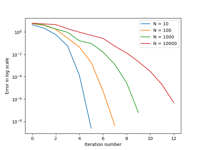
In our implementation of the algorithm, the intersection of power diagrams with a paraboloid is computed using an algorithm presented in [13]. Once the diagram is computed, the function $H$ and its differential $DH$ are computed using the trapezoidal rule. Numerical experiments are performed with $X=[-1,1]^{2}$ and $\mu$ equal to (one fourth) of the restriction of the Lebesgue measure on $X$ . The set $Y$ is randomly generated in the square $[0,1]^{2}$ for different values of $N$ , associated with a discrete uniform measure $\nu$ . Figure 2 (left) shows the initial diagram $(\mathrm{Lag}_{i}(\psi))_{1\leq i\leq N}$ with $N=5000$ for some vector $\psi=\lambda\mathrm{\textbf{1}}$ with $\lambda>0$ . Figure 2 (right) is the same diagram after convergence of the algorithm, where $\psi$ is an approximate solution of (NF paral). The graph of Figure 3 represents the error $\|H(\psi^{k})-\nu\|_{1}$ as a function of iteration $k$ . It shows superlinear convergence of the damped Newton method.

Refer to caption — Figure 2. Initial diagram for $N=5000$ , and final diagram, after convergence of the algorithm.

Acknowledgements

We acknowledge the support of the French Agence Nationale de la Recherche through the project MAGA (ANR-16-CE40-0014).

References

[1] Farhan Abedin and Cristian E Gutiérrez. An iterative method for generated jacobian equations. Calculus of Variations and Partial Differential Equations, 56(4):101, 2017.
[2] Robert J Berman. Convergence rates for discretized monge–ampère equations and quantitative stability of optimal transport. Foundations of Computational Mathematics, pages 1–42, 2020.
[3] Jean-Daniel Boissonnat, Camille Wormser, and Mariette Yvinec. Curved voronoi diagrams. Effective Computational Geometry for Curves and Surfaces, 01 2007.
[4] Luis A Caffarelli, Sergey A Kochengin, and Vladimir I Oliker. Problem of reflector design with given far-field scattering data. In Monge Ampère equation: applications to geometry and optimization, volume 226, pages 13–32, 1999.
[5] Alfred Galichon, Scott Duke Kominers, and Simon Weber. Costly concessions: An empirical framework for matching with imperfectly transferable utility. Journal of Political Economy, 127(6):2875–2925, 2019.
[6] Nestor Guillen. A primer on generated jacobian equations: Geometry, optics, economics. Notices of the American Mathematical Society, 66:1, 10 2019.
[7] Nestor Guillen and Jun Kitagawa. Pointwise estimates and regularity in geometric optics and other generated jacobian equations. Communications on Pure and Applied Mathematics, 70(6):1146–1220, 2017.
[8] Cristian E Gutiérrez and Federico Tournier. Regularity for the near field parallel refractor and reflector problems. Calculus of Variations and Partial Differential Equations, 54(1):917–949, 2015.
[9] Feida Jiang and Neil S Trudinger. On pogorelov estimates in optimal transportation and geometric optics. Bulletin of Mathematical Sciences, 4(3):407–431, 2014.
[10] Jun Kitagawa. An iterative scheme for solving the optimal transportation problem. Calculus of Variations and Partial Differential Equations, 51(1-2):243–263, 2014.
[11] Jun Kitagawa, Quentin Mérigot, and Boris Thibert. Convergence of a newton algorithm for semi-discrete optimal transport. Journal of the European Mathematical Society, 21(9):2603–2651, 2019.
[12] Sergey A Kochengin and Vladimir I Oliker. Determination of reflector surfaces from near-field scattering data. Inverse Problems, 13(2):363, 1997.
[13] Pedro Machado Manhães De Castro, Quentin Mérigot, and Boris Thibert. Far-field reflector problem and intersection of paraboloids. Numerische Mathematik, 134(2):389–411, 2016.
[14] Quentin Mérigot, Jocelyn Meyron, and Boris Thibert. An algorithm for optimal transport between a simplex soup and a point cloud. SIAM Journal on Imaging Sciences, 11(2):1363–1389, 2018.
[15] Quentin Merigot and Boris Thibert. Optimal transport: discretization and algorithms. In Handbook of Numerical Analysis, volume 22. Elsevier, to appear, 2021.
[16] Georg Nöldeke and Larry Samuelson. The implementation duality. Econometrica, 86(4):1283–1324, 2018.
[17] VI Oliker and LD Prussner. On the numerical solution of the equation $\frac{{\partial^{2}z}}{{\partial x^{2}}}\frac{{\partial^{2}z}}{{\partial y^{2}}}-\left({\frac{{\partial^{2}z}}{{\partial x\partial y}}}\right)^{2}=f$ and its discretizations, I. Numerische Mathematik, 54(3):271–293, 1989.
[18] Vladimir Oliker. Mathematical aspects of design of beam shaping surfaces in geometrical optics. In Trends in Nonlinear Analysis, pages 193–224. Springer, 2003.
[19] Neil S Trudinger. On the local theory of prescribed jacobian equations. Discrete & Continuous Dynamical Systems-A, 34(4):1663–1681, 2014.

A Damped Newton algorithm for Generated Jacobian Equations

Abstract.

1. Introduction

Semi-discrete optimal transport.

Generated Jacobian equation.

2. Semi-discrete generated Jacobian equation

2.1. Generating function

Definition 1 (Generating function).

Remark 2 (Range of GG).

Remark 3.

Definition 4 (G-convexity).

Remark 5 (Relation with convexity).

Definition 6 (G-subdifferential).

Lemma 7.

Definition 8 (Brenier solution to the GJE).

2.2. G-transform

Definition 9.

Proposition 10.

Proof.

Corollary 11.

Remark 12 (GG-convex functions are not always GG-transforms).

Definition 13 (Generalized Laguerre cells).

Definition 14 (Alexandrov solution to GJE).

3. Resolution of the generated Jacobian equation

3.1. 𝒞1\mathcal{C}^{1}-regularity of HH

Definition 15 (Genericity of the generating function.).

Proposition 16.

Proof.

Proposition 17.

Proof.

3.2. Kernel and image of D​H\mathrm{D}H

Proposition 18.

Lemma 19.

Proof.

Lemma 20.

Proof.

Proof of Proposition 18.

Remark 21.

3.3. Damped Newton algorithm

Lemma 22 (Admissible set).

Proof.

Proposition 23 (Newton’s direction).

Proof.

Theorem 24 (Linear convergence).

Proof.

Remark 25 (Existence).

4. Application to the Near Field Parallel Reflector problem

4.1. Generated Jacobian equation.

Proposition 26.

Proof.

4.2. Laguerre and Möbius diagram.

Definition 27 (Möbius diagram).

Proposition 28.

Theorem 29.

Remark 30.

4.3. Implementation.

Definition 31 (Power diagram).

Proposition 32.

Acknowledgements

References

Remark 2 (Range of $G$ ).

Remark 12 ( $G$ -convex functions are not always $G$ -transforms).

3.1. $\mathcal{C}^{1}$ -regularity of $H$

3.2. Kernel and image of $\mathrm{D}H$