TTK-21-03
Electric dipole moment of the tau lepton revisited
Werner Bernreuther a,11 1 breuther@physik.rwth-aachen.de, Long Chen a,22 2 longchen@physik.rwth-aachen.de and Otto Nachtmann b,33 3 o.nachtmann@thphys.uni-heidelberg.de
aInstitut für Theoretische Teilchenphysik und Kosmologie,
RWTH Aachen University, 52056 Aachen, Germany
b Institut für Theoretische Physik, Universität Heidelberg, 69120 Heidelberg, Germany
Abstract
We reconsider the issue of the search for a nonzero electric dipole form factor (EDM) using optimal observables in production by collisions in the center-of-mass energy range from the -pair threshold to about GeV. We discuss the general formalism of optimal observables and apply it to two -odd observables that are sensitive to the real and imaginary part of , respectively. We compute the expectation values and covariances of these optimal observables for -pair production at GeV with subsequent decays of into major leptonic or semihadronic modes. For the decays to two pions and three charged pions we take the full kinematic information of the hadronic system into account. Assuming that the Belle II experiment at the KEKB accelerator will eventually analyze data corresponding to an integrated luminosity of 50 ab-1 and applying acceptance cuts on the final-state pions we find that 1 s.d. sensitivities and can be obtained with events where both ’s decay semihadronically. We consider also the ideal case that no cuts on the final-state particles are applied. With 50 ab-1 at GeV corresponding to events we find the 1 s.d. sensitivities and , again for events where both leptons decay semihadronically. Furthermore, we analyze the potential magnitude of the EDM form factor in the type-II two-Higgs doublet extension and in two scalar leptoquark extensions of the Standard Model, taking into account phenomenological constraints.
1 Introduction
The search for electric dipole moments (EDMs) of fundamental fermions is an important aspect of experimental investigations hunting for physics beyond the Standard Model (SM) of particle physics, in particular for violation beyond the Kobayashi-Maskawa mechanism. So far only upper bounds for these EDMs exist [1]. For the electron an impressive upper limit was obtained rather recently by the ACME Collaboration [2]. The best muon EDM limit to date was set by the Muon Collaboration [3]. These limits are
| (1) | ||||
| (2) |
The lifetime of the lepton is too short to allow for the measurement of its static moments. Instead information on the nonstatic EDM form factor11 1 In this paper we use the acronym EDM for both the static moment and the form factor at . can be retrieved, for instance, from the measurement of -violating correlations in -pair production by collisions. The EDM form factor can be a complex quantity for timelike momentum transfer. The best limits to date on its real and imaginary parts were obtained by the Belle I Collaboration [4] at :
| (3) |
In a series of articles where two of the authors of this paper were involved, ways of searching for -violating effects in collisions, in particular for a nonzero EDM, were proposed [5, 6, 7, 8, 9]. The observables and results of [6, 9] were used in the experimental searches for an EDM form factor of the lepton by [4] and earlier by the ARGUS Collaboration [10] that obtained the results
| (4) |
at a c.m. energy of the reaction . For reviews of the search results for the EDM and its weak dipole form factor (the analogue of the EDM for the coupling of the Z boson to fermions); see, for instance, [11, 12]. Further discussions of possible measurements of the anomalous magnetic moment and the EDM of the lepton can be found in [13, 14, 15, 16, 17] and references therein.
The experimentation at Belle II [18] which started recently at the KEKB accelerator offers new possibilities for measuring the EDM form factor, in particular, because a huge number of recorded -pair events are expected at the end of data taking [19]. Also the BES III experiment, where collisions at a center-of-mass (c.m.) energy GeV are studied, expects to collect and analyze a large number of pairs [20]. Therefore, we reconsider the issue with particular emphasis on using optimal observables [21, 22, 23] for tracing the EDM form factor in -pair production at c.m. energies from threshold up to about 15 GeV where the contribution from -boson exchange is negligible. In our numerical analysis we consider -pair production at GeV. Moreover, we analyze this form factor in a few SM extensions that can induce a potentially sizable EDM [24].
Our paper is organized as follows. In Section 2 we recall the form factor decomposition of the vertex and in particular the definition of the EDM form factor. In section 3 we discuss the production and decay matrices for the process with the ’s decaying into one, two, or three particles that are measured in an experiment. Section 4 deals with simple and optimal observables [21, 22, 23] for tracing the EDM of the lepton. Section 5 contains our numerical results, in particular our estimates of the sensitivities with which the real and the imaginary parts of the EDM form factor can be measured in various decay channels. In Section 6 we consider the EDM form factor in a type-II two-Higgs doublet extension and in two leptoquark extensions of the SM and analyze the potential magnitude of the EDM taking into account experimental constraints. Moreover, we show that within these models -violating box contributions to the -matrix element of are negligible as compared to that of the EDM form factor. We conclude in Section 7. In Appendix A we list the density matrices for several major decays of polarized leptons. In particular, we present the explicit form of the differential decay density matrices for and . Appendix B contains a detailed analysis of the expectation values and covariances of the -odd optimal observables used in Sec. 5 in various decay channels.
2 Form Factors
We consider production in collisions at c.m. energies from threshold up to about 15 GeV, with and decaying into a final state and , respectively,
| (5) |
The four-momenta and the corresponding three-momenta are denoted in the c.m. frame by , . We consider unpolarized electrons and positrons and neglect their masses; the labels denote the spin indices of the tau leptons. In the c.m. frame we have .
For unpolarized and the initial state is described by a -invariant density matrix. Thus, any non zero -odd correlation observed in the final state indicates a genuine -violating effect that can be located in the production and/or in the decays of the ’s. We consider tau-pair production by one-photon-exchange only. At the energies considered here -boson exchange is negligible. This will be justified at the end of this section. The diagram shown in Fig. 1 exhibits this approximation with the full photon propagator
| (6) |
where is the vacuum-polarization function; see e.g. Eq. (19.45) of [25]. For instance, at the mass of the resonance, at GeV, this vacuum polarization effect produces an enhancement of the cross section. For a detailed discussion of the -pair cross section at this energy, including radiative corrections, we refer to [26]. Below we consider only normalized expectation values of observables where such resonance enhancements enter only through the number of events which we take as input from experiment.
In the following we assume that the only source of violation in the diagram of Fig. 1 is due to a nonzero EDM form factor in the vertex. This vertex is given by the following one-particle irreducible (1PI) matrix element of the electromagnetic current between the vacuum and the final state:
| (7) |
where . The right-hand side of (2) represents the most general decomposition of this matrix element taking into account the conservation of the electromagnetic current. Moreover, denotes the charge and we use the -matrix conventions of [25]. Note that the order of and in the matrix element (2) matters because we are dealing with fermions. The form factors , and are analytic functions of in the complex plane with a cut on the positive real axis satisfying
| (8) |
That is, on the real axis, the form factors are real functions for and can have imaginary parts for . At higher order in these cuts start at due to cut diagrams of the type shown in Fig. 2 with three photons in the intermediate state. In the decomposition (2) we have and we have to set , that is, to take above the cut.
Next we recall the transformation properties of the coupling terms associated with the four form factors in (2) under charge conjugation (), parity (), and . Assuming that the interaction is invariant under these transformations and using the transformation of under , , and , one gets the transformation properties listed in Table 1.
The amplitude can receive also -odd 1PI box contributions, for instance contributions with Lorentz structure . We do not take such contributions into account in the following. We discuss a few SM extensions in Section 6 that can induce sizable EDM form factors. For these models we show in Section 6.3 that the -violating box contributions can be neglected as compared to that of the induced EDM form factor.
For the matrix elements of the current between and states, respectively, we get, using the standard crossing relations:
| (9) |
| (10) |
where the vertex function is given by the expression in the square brackets of Eq. (2) with and
The form factor is the electric or Dirac form factor with the normalization
| (11) |
The magnetic or Pauli form factor at yields the anomalous magnetic moment:
| (12) |
The and electric dipole moments, respectively, are obtained from the EDM form factor at :
| (13) |
The form factor at defines the anapole moment [27, 28, 29, 30] of the :
| (14) |
For a at rest, , one has
| (15) |
A comment on the gauge invariance of the form-factor decomposition of the vertex function (2) is in order. Electromagnetic gauge invariance is obvious, because conservation of the electromagnetic current was used in the decomposition of (2). As to the invariance with respect to the electroweak gauge group : The static moments at , in particular the anomalous magnetic and electric dipole moment and the anapole moment are gauge invariant, as they correspond to terms in the -matrix element in the soft-photon limit. Yet, for obtaining a gauge-invariant amplitude for one cannot, of course, use (2) in isolation, but must take into account all contributions (including box contributions at one-loop order and beyond) to the -matrix element order by order in the electroweak couplings. However, in the following we use only the tree-level vertex supplemented by the EDM form factor. The EDM is extremely small in the SM, as will be briefly reviewed at the beginning of Section 6. Thus, a sizable value for must come from “beyond the Standard Model” (BSM) physics. In Section 6 we discuss a few BSM extensions that can induce a sizable EDM form factor and compute it at one-loop order. The form factors given in that section are invariant with respect to the electroweak gauge group.
As is well-known one may introduce a EDM, together with an analogous -violating weak dipole moment (WDM) in the vertex, by using a invariant effective Lagrangian approach for BSM couplings. Imposing baryon and lepton number conservation the leading gauge-invariant operators have mass dimension 6 [31] and the relevant effective Lagrangian takes the form (see, for instance, [32]):
| (16) | |||||
Here and are dimensionless real coupling constants, denotes the energy scale of new physics that is assumed to be considerably larger than the electroweak symmetry breaking scale GeV, and are the and gauge couplings, respectively, and are the gauge field strength tensors corresponding to these groups, is the Higgs doublet field, and and are the right-handed singlet and left-handed lepton doublet fields of the third generation. (Our notation follows [33].) After spontaneous symmetry breaking the effective Lagrangian (16) contains the EDM interactions
| (17) |
where and are, respectively, the Abelian field strength tensors of the photon and boson and and the electric and weak dipole moments of the lepton:
| (18) |
This approach constitutes a possibility to introduce the EDM and WDM in a way that respects electroweak gauge invariance. Using the Hermitian Lagrangian (17) to leading order corresponds to setting
| (19) |
and likewise for . In this framework imaginary parts of and will be generated by diagrams involving both of Eq. (17) and SM couplings at higher order. We shall take into account in the following that can be nonzero for but we neglect, as already mentioned above, the contribution from -boson exchange, in particular the contribution from . This can be justified as follows. Eq. (18) shows that and will be of the same order of magnitude if the coupling constants and are of comparable size. This is the case, for instance, in the BSM models considered in Section 6, as was shown in [24]. At energies that we consider in this paper, the effects of resulting from -boson exchange are then negligible compared to those of , as is the contribution resulting from the interference of the SM -boson exchange amplitude with the amplitude involving . One can see this explicitly from the formulas given in [9] where both and -boson exchange were taken into account. From Eq. (3.10) of [9] we find that for c.m. energies GeV that we are considering -boson exchange contributions are suppressed by a factor of order
| (20) |
This holds for in the continuum and at the resonance where the suppression factor (20) is a few percent smaller because there the photon contribution is enhanced as compared to the continuum value; see [26].
3 Matrix elements, production and decay matrices
We are interested in analyzing -violating effects in -pair production generated by a nonzero EDM form factor. Therefore we shall analyze the reactions (5) by considering on-shell -pair production by one-photon exchange, including the EDM form factor in the vertex, followed by the decays of and into the final states and , respectively. The spin correlations and polarizations will be taken into account. (The reactions (5) were investigated in [9] for arbitrary c.m. energies for photon and -boson exchange including besides the EDM also the weak dipole form factor of the lepton.)
As to the decay channels and , we consider two cases:
i) Only one charged particle of and one of are measured:
| (21) |
Examples from the main decay modes of are
| (22) |
and the respective charge-conjugate decays. The decay modes (3) include, in particular,
decays to one charged prong.
ii) We shall also treat the case where more than one particle from decay is observed,
specifically the decay to two pions via a and meson and
the decay to the meson, respectively to three charged pions:
| (23) | ||||||
| (24) |
For on-shell -pair production and decay the cross section of (5) can be written as a product of the production density matrix for times the density matrices and that describe the decays of polarized and , respectively. The production density matrix is defined as follows:
| (25) | |||||
where are the spin indices of and , respectively. For a decay of according to case i) above the corresponding decay density matrix is given by
| (26) | |||||
Here the normalization is chosen such that
| (27) |
where is the mean multiplicity of particle in channel . Formulas analogous to (26) and (27) apply if decays according to case i) are considered.
Thus the cross section for the two-particle inclusive reactions
| (28) |
where
| (29) |
is given in the narrow-width approximation of the intermediate leptons by
| (30) |
where , the solid angle element corresponds to the momentum vector in the c.m. frame, and and denote the branching fractions for the decays and , respectively.22 2 Formula (4.3) of Ref. [9] contains a typo. These branching fraction factors are missing. However, they were taken into account in the numerical results given in that paper. Moreover, the variable on the l.h.s. of Eq. (4.4) of that reference should be replaced by .
For decay to three charged pions whose four-momenta are all measured in an experiment we define the corresponding decay density matrix by
| (31) |
where is the four-momentum of , and analogously for the decay . The normalization is
| (32) |
corresponding to the multiplicity in this channel. If the analysis is restricted to three pions in a suitably defined invariant mass region around the nominal mass one has to take into account the corresponding phase-space cuts in and in (32).
For the decay (23) to two pions, where both the charged and the neutral pion are measured, the respective decay density matrix is defined accordingly by integrating the corresponding squared matrix element over the four-momentum of the neutrino.
In order to get the inclusive cross section for case ii), considering, for instance, the decay of the into three observed pions, we have to make in (3) the replacement
| (33) |
Analogous replacements apply if the decay of to three observed pions or the decay of to two observed pions are analyzed.
The production density matrix in (3) is computed in the c.m. system, see below. Instead of calculating the decay density matrices also in this frame we can determine them in the and rest systems, respectively, if we use the following:
- •
We consider rotation-free Lorentz transformations (boosts) from the c.m. frame to the and rest systems, respectively.
- •
We use standard spinors , for the ’s with denoting the spin components in a given direction (see, e.g., [33]).
As is well known, these spin components are not changed by boost transformations. Let be the boost transforming the momentum from the c.m. system to rest, , where We have then with ; see (153) and (154),
| (34) |
Insertion into the decay matrix (26) proves our statements above. The analogous argumentation applies to the decay density matrices.
In Appendix A we give the explicit forms of the decay density matrices in the respective rest frames for the decay modes listed in (3) – (24).
Finally, using the one-photon-exchange approximation and setting
| (35) |
the production density matrix is given in the c.m. frame by
| (36) |
where [9]
| (37) |
and
| (38) | |||||
| (39) | |||||
| (40) | |||||
| (41) |
Compared to Eqs. (3.8) – (3.10) of [9] we neglect here the contributions from -boson exchange because we restrict ourselves to the kinematic range , but we have included the photon vacuum polarization effects. In (38) – (41) we put , and and denote the respective unit vectors. We have introduced in (37) and (41) dimensionless EDM form factors defined by
| (42) |
Moreover, we use in the equations above the notation [9]
| (43) |
where the first and second factors in these tensor products refer to the spin spaces of and , respectively. The density matrices and are -even, whereas is - and -odd while is -odd and -even. Here and below -even/odd refers to the behavior with respect to the naive “time reversal” transformation, that is, reflections of three-momenta and spins.
Equation (39) shows that a nonzero generates -odd spin correlations in the scattering plane while a nonzero imaginary part of leads to a -odd asymmetry of the and polarizations with projections along and , cf. (40). The leptons autoanalyze their spin directions via their parity-violating weak decays. In this way these spin correlations and polarization asymmetries induce -odd angular correlations among the decay products, to which we now turn.
4 Simple and optimal observables
In this chapter we discuss simple and optimal observables for studying violation in the reactions (5). Let us first consider the case i) above where only one charged particle is measured from and decay, respectively, i.e., and . Simple observables for this case were given in Ref. [9]. Observables sensitive to are, for instance, the tensors
| (44) |
| (45) |
Observables sensitive to are, for instance,
| (46) |
| (47) |
The momenta in (44) – (47) are defined in the c.m. frame, and and are the Cartesian vector indices. These observables, denoted generically by , have the property to be odd under :
| (48) |
Moreover, Eqs. (44) and (45) are -odd while (46) and (47) are -even. A nonzero expectation value of any such observable of the form
| (49) | |||||
is a genuine signature of violation. Here is the cross section (3) of the reaction (28) and the corresponding one for the charge-conjugate channel. We assume that any phase-space cuts that may be applied are made in a -symmetric way.
Observables of the type (44)-(47) were studied extensively in [9]. In Sec. 5 we give an update of the sensitivities achievable with these observables at the KEKB accelerator with Belle II. A discussion of the sensitivities achievable with the BES III experiment at the Beijing Electron-Positron Collider II is deferred to a future publication.
We shall now turn to optimal observables [21, 22, 23] and we follow here Ref. [23]. We denote the measured phase-space variables generically by and the -transformed ones by :
| (50) |
Phase-space cuts are assumed to be -symmetric. In the following we denote the dimensionless -violating EDM form factors (cf. Eq. (42)) that are to be measured by
| (51) |
From experiment we know that these couplings are small, . From (1) we get for GeV. Therefore, we shall work to leading order in these couplings. The cross section (3) can be expanded in the as follows, neglecting terms of second order in these couplings:
| (52) |
Here and in the following we use the summation convention. Moreover, in order not to overload the notation, the labels and denote in (52) and in what follows decays of and to one, two, or three measured particles, respectively. The properties of and in (52) are:
| (53) |
We define now the observables
| (54) |
Their expectation value for is
| (55) |
We set
| (56) |
and get for the expectation value of :
| (57) |
The expression on the right-hand side is obtained by expanding the ratio to first order in the . Here is the covariance matrix of the quantities for .
| (58) |
The covariance matrix is positive definite. From (57) we obtain
| (59) |
In the remainder of this section we recall from [23] some general relations for optimal observables in order to make our article self-contained. Also, we shall discuss that in the nondiagonal case the theoretically optimal estimators may not always be “optimal” from a practical point of view (see the discussion after Eq. (78) below).
We consider first the diagonal case, , and assume that events of this type are analyzed. The density function is then
| (60) |
The information matrix is defined by
| (61) |
The optimal estimators for the couplings are in this case:
| (62) |
where denotes the mean value of . From Eqs. (59) and (4) we obtain the expectation values
| (63) |
and the covariance matrix of the , evaluated for , is
| (64) |
We get for the information matrix (61):
| (65) |
Therefore, we have here
| (66) |
and the estimators (62) are optimal for small . That is, the error ellipse obtained with the estimators in (62) is given by the one obtained from which is the smallest one possible. We note that due to the properties (53) of and we have in the diagonal case , assuming possible cuts in phase space to be -symmetric:
| (67) |
and the optimal estimators are
| (68) |
Finally, we treat the nondiagonal case, . We assume that any phase-space cuts made for the channel are applied to in a -conjugate way. We get then from the relations (53):
| (69) |
| (70) |
| (71) |
We assume that events of the type and events are analyzed. The density function is then
| (72) |
with
| (73) |
Here the information matrix is given for by
| (74) |
where . Here it is convenient to use as estimators for the couplings , with from (54):
| (75) |
We have
| (76) |
The covariance matrix of these estimators is obtained as
| (77) |
which implies
| (78) |
The in Eq. (75) are the optimal estimators for . For they are not quite optimal, but for the theoretically optimal estimators one would need in this case the precise knowledge of . This would introduce an unnecessary source of uncertainty in the measurements.
To conclude this section we remark on the following. A more elaborate description of -pair production and decay would take higher-order radiative corrections into account. Let us denote the resulting differential cross section by ,
| (79) |
If it is -invariant, we have
| (80) |
Then the corresponding expectation values of the estimators defined in (68) and (75) and constructed with the expressions , from (52) will, of course, be zero due to (53):
| (81) |
That is, the observables given in (68) and (75) are in all cases genuine observables. They cannot get nonzero expectation values, neither from -conserving radiative SM corrections nor from -conserving interactions beyond the SM.
5 Numerical results at GeV
We consider now -pair production and decay at the resonance at and compute the expectation values of the simple and optimal observables discussed in the previous section and estimate the resulting 1 s.d. (standard deviation) statistical sensitivities to the EDM form factors and at this c.m. energy. The expectation values of the observables are computed to leading order in the real and imaginary parts of the EDM form factor using the expression (3) for the differential cross section with (35) – (40) and several of the decay density matrices given in Appendix A. First, no phase-space cuts are applied. At the end of this section we analyze also the effects of cuts.
The expectation values of the observables (44) – (47) at the resonance in the decay channels where only one charged particle from and one from decay is measured (case i) above) are of the form:
| (82) | |||||
| (83) |
In the case of nondiagonal decay channels the expectation values are calculated as averages defined in (49). The expectation values of the symmetric traceless tensors (44) – (47) must be proportional to a tensor with the same property. Using the beam direction in the c.m. frame we have
| (84) |
The right-hand side of (84) follows from identifying with the axis which we do in the following. Equation (84) is identical to the tensor polarization of the intermediate photon state. Because the diagonal elements of the above tensor observables are not independent, we consider only their components that have the largest expectation values. Naive “time reversal” invariance implies that the expectation values (82) and (83) do not depend on and , respectively. That is, the covariance matrix of the and tensors is diagonal; see Appendix B.
In order to estimate the statistical error in the measurement of the expectation values of the observables we compute also the respective standard deviation of the distribution of in the SM for the various decay channels. As discussed in Appendix B the SM expectation values of the tensors , vanish for the differential cross section as used by us. (Cf. Section 3.) For the tensors , this is also true in the diagonal case . In the nondiagonal case, , their SM expectation values need not be zero, but are found numerically to be negligibly small. In Tables 2 and 3 we assume that the momenta of mesons can be experimentally determined and we treat them as on-shell particles with the -spin analyzing power given in (119). The symbols and denote either the electron or muon, both are taken to be massless. We sum over the diagonal and nondiagonal channels for estimating the respective sensitivity to the real and imaginary parts of the EDM. In a diagonal decay channel the number of events is , while for a nondiagonal channel including its charge-conjugate mode we have . The branching ratios are taken from [1]. We assume that the Belle II experiment will eventually record pairs [19]. Considering as an example the measurements of and in the decay channels and the resulting ideal 1 s.d. statistical errors of the dimensionful EDM couplings and are given by
| (85) |
Equation (85) yields the absolute value that must have in order that deviates from its SM prediction, namely zero, by 1 s.d. obtained from the square root of its SM variance. Formulas analogous to (85) hold for the dimensionless observables and .
Tables 2 and 3 contain our results for the expectation values (as defined in Eqs. (82) and (83)) and square roots of the variances of the observables (44) – (47) for several one-prong decays of where the charged particle has a sizable -spin analyzing power. Moreover, the resulting 1 s.d. sensitivities to the real and imaginary parts of the EDM form factor are listed.33 3 The last digit of the expectation values and variances listed in Tables 2, 3, and 4 is rounded. The sensitivities and listed in these tables are computed with these rounded numbers. Results for and were previously given in [9] and agree with those in Tables 2 and 3. The accuracies and attainable in the various decay channels listed in Tables 2 and 3 show that the dimensionful observable is more sensitive than while in the case of and it is the other way around – except for the decay channel which has, in any case, a rather poor sensitivity compared to the other decay modes.
Next we apply the optimal observables (54) for measuring and to the reactions of Sec. 3. As in Eq. (52) and in the following equations, the labels refer here to the decays of and/or to one, two, or three measured particles. In particular, we take now the differential decay density matrices for and given in Appendix A into account. Using (38), (39), and (40) and the respective decay matrices and we define
| (86) |
where the trace is taken with respect to the spin indices of and . Both observables are -odd and is also -odd while is -even. As already emphasized we compute the expectation values by integrating over the whole phase space. According to the general theory discussed in Sec. 4 and Appendix B the covariance matrix for a decay channel is given, for zero EDM, by (58), (71):
| (87) |
where
| (88) |
etc., denote the expectation values for . The expectation values for nonzero EDM are given by (4):
| (89) |
We get for the covariance matrix of the optimal estimators of and ; see (62), (64) and (75), (77):
| (90) |
Here is the number of events in the diagonal channels whereas for it is the sum of the events and , assuming that their numbers are equal.
However, with the form of the differential cross section used in this paper considerable simplifications occur. In the case where the leptons decay to one measured particle and/or to where both pions are measured we have, as shown in Appendix B:
| (91) |
That is, for these channels the respective covariance matrix (87) is diagonal.
When , , or both leptons decay to three measured pions, still holds in the one-photon approximation (see Appendix B), but the covariance matrix is no longer diagonal. Yet we find for these decay modes that with numerical uncertainties below . Therefore, within the precision of our numerical analysis the relations (91) hold also for these decay channels, and (89) simplifies to44 4 The left-hand sides of (92) denote averages according to (49).
| (92) |
where we used the abbreviations
| (93) |
The resulting 1 s.d. errors of the dimensionful EDM couplings and are given by
| (94) |
Table 4 contains our results for the expectation values defined in Eq. (92) and for the square roots of the variances of the observables (86) for several decays to one, two and/or three measured particles. The numbers in this table show that taking into account the full kinematic information on the hadronic system in the and decays results in maximal -spin analyzing power [34, 35], as is the case in the decay . In addition, the resulting 1 s.d. sensitivities to the real and imaginary parts of the EDM form factor are given in Table 4, assuming again -pair events. The 1 s.d. statistical errors and exhibited in Table 4 signify that taking into account the channels where one or both leptons decay to two and/or three measured pions yields a significant improvement in the sensitivity to the EDM form factor. Comparing for each channel the accuracies and exhibited in Table 4 with those in Tables 2 and 3 shows that, as expected, the optimal observables (86) are significantly more sensitive to the EDM than the observables and .
If the measurement errors of the various exclusive decay modes are uncorrelated, we may add in quadrature the statistical errors of and attainable for each channel:
| (95) |
and analogously for . Performing these quadratures with the uncertainties listed in Tables 2, 3, and 4 yields the 1 s.d. errors and given in Table 5. As to the optimal observables we assumed here for the purpose of comparison that they are measurable for all channels listed in Table 4. For the leptonic modes this may not be possible in an unambiguous way; see below. The numbers in Table 5 show that the sensitivity to is improved by a factor of about 6 with the optimal observable as compared to using the simple ones, whereas the sensitivity to is improved by a factor of about 4.
We briefly discuss the measurability of the observables used in this section.
The KEKB accelerator is an asymmetric collider; particle momenta measured in
the laboratory frame can of course be transformed to the c.m. frame.
The simple observables (44) – (47) applied to the decay channels
listed in Tables 2, 3 require the momenta of charged mesons and of in the
c.m. frame. They can be straightforwardly measured, except for the momentum of whose
determination requires
the reconstruction of the decay .
The optimal observables involve the momenta of various particles from decay in the
respective rest frame.
This requires
the knowledge of the momenta in the c.m. frame. If both and decay
semihadronically their momenta can be
reconstructed in an unambiguous way [36]. If one of the leptons decays semihadronically and
the other one to either or , one
may discard radiative events in this class such that the and in the remaining events are,
to good approximation, back to back
and carry half of the c.m. energy in the frame. If the momentum can
be reconstructed in the semihadronic decay, e.g. by reconstructing
the production and decay vertices, the momentum of the leptonically decaying can be inferred. If both leptons decay
leptonically the determination of their momenta is not possible in an unambiguous way.
Therefore, we discard the results for the channels in Table 4
and add in quadrature the statistical errors of and
attainable with the events listed in Table 4 where both ’s decay semihadronically
and for the case where the semihadronic-leptonic decays of
are added to the purely semihadronic events. The resulting 1 s.d. errors are given in Table 6.
The numbers in this table and in Table 5 show that restriction to purely semihadronic
decays does not lead to a significant decrease in sensitivity to and .
Next we investigate the effects of cuts on the sensitivities to the EDM. A full-fledged Monte Carlo analysis with detailed cuts is beyond the scope of this paper. We analyze in the following only the expectation values of the optimal observables in the channels where both leptons decay semihadronically, as these observables and decay modes appear to have the highest sensitivity to and allow for an unambiguous reconstruction of the momenta. We apply the following -invariant phase-space cuts on the final-state pions in the c.m. frame:
| (96) |
where is the polar angle of a pion with respect to the beam and its transverse momentum.55 5 The cut on is inspired by the acceptance of the Belle II detector in the KEKB laboratory frame [19]. Table 7 contains the resulting coefficients and of the expectation values of and , respectively, defined in (92). The event numbers and sensitivities given in Table 7 are estimated by assuming an integrated luminosity of that corresponds to assuming in the case of no cuts. The expectation values are somewhat increased by the cuts while the event numbers are, of course, diminished. The resulting overall sensitivities are given in Table 8. Comparing these numbers with those of Table 6 shows that the cuts (96) lead only to a slight decrease in sensitivity to the EDM.
Moreover, the following remark is in order. As already indicated below Eq. (6) our results for the normalized expectation values listed in Tables 2, 3, 4, and 7 do not depend on the fact that there is a resonance enhancement at GeV; these numbers hold also for the direct continuum production of pairs. In addition, we emphasize again that the event numbers, respectively the integrated luminosity that we use for our sensitivity estimates to the EDM are expectations taken from [19].
The sensitivity to the EDM that the Belle II experiment may eventually achieve with purely semihadronic decays was investigated also in [16]. The authors of this paper use the term proportional to of the matrix element for as optimal observable. It is evaluated with the momenta of the mesons and the reconstructed one of the neutrinos. The real and imaginary parts of the EDM are not separately determined. Assuming the same event number as we did above, the authors of Ref. [16] find that a 1 s.d. statistical sensitivity can be achieved with their approach.
6 The EDM form factor in some SM extensions
In the SM the EDM of a charged lepton is extremely tiny and generated only at high loop order. The dominant short-distance contribution to is thought to arise via Kobayashi-Maskawa phase induced four-loop contributions that contain, for instance, the induced EDM form factor of the boson. It can be estimated to be of the order . (One may take, for instance, the estimate of [37] for and apply it to the lepton.) Recently it was pointed out that long-distance hadronic contributions are considerably larger [38]. For the EDM is was found that these contributions amount to [38]. Nevertheless, this is undetectable for the time being.
Thus, the detection of a nonzero particle EDM, in particular of the lepton, in a present-day experiment or one in the foreseeable future would be evidence for a new type of violation. In this section we consider three SM extensions with -violating interactions that generate EDM form factors of fundamental fermions already at one loop. The models we are interested in have -violating Yukawa couplings. These interactions can induce a EDM that can be much larger than the electron EDM generated in these models.66 6 We recall that in models with Higgs-Yukawa-like -violating couplings the dominant contribution to the electron EDM occurs at two loops [39]. We compute the EDM at one loop in a type-II two-Higgs-doublet model and in two scalar leptoquark models and investigate its potential magnitude in the timelike region , taking into account phenomenological constraints, in particular the tight upper bound (1) on the electron EDM.
6.1 Type-II two-Higgs doublet extension
In two-Higgs doublet models (2HDM) the field content of the SM is extended by an additional Higgs doublet . We consider here as an example the so-called type-II model. It is defined by its Yukawa coupling structure: the doublet is coupled to right-chiral down-type quarks and charged leptons, while is coupled to right-chiral up-type quarks only. By construction, flavor-changing neutral currents are absent at tree level in this model. Assuming a -violating Higgs potential the particle spectrum of the 2HDM contains three neutral Higgs bosons that are mixtures. In flavor-conserving 2HDM their Yukawa couplings to quarks and leptons are of the form
| (97) |
where , is the Fermi constant, and the reduced Yukawa couplings and depend on the specific type of 2HDM. In the type-II model the reduced couplings of the mass eigenstates to the lepton are (we use here the conventions of [40]):
| (98) |
Here is the ratio of the vacuum expectation values of the two Higgs doublet fields, and is a real orthogonal matrix that relates the eigenstates and the mass eigenstates of the three physical neutral Higgs bosons. The relations (98) hold also for the other charged leptons and the down-type quarks. (For up-type quarks, see for instance [40].) If then (97) violates .
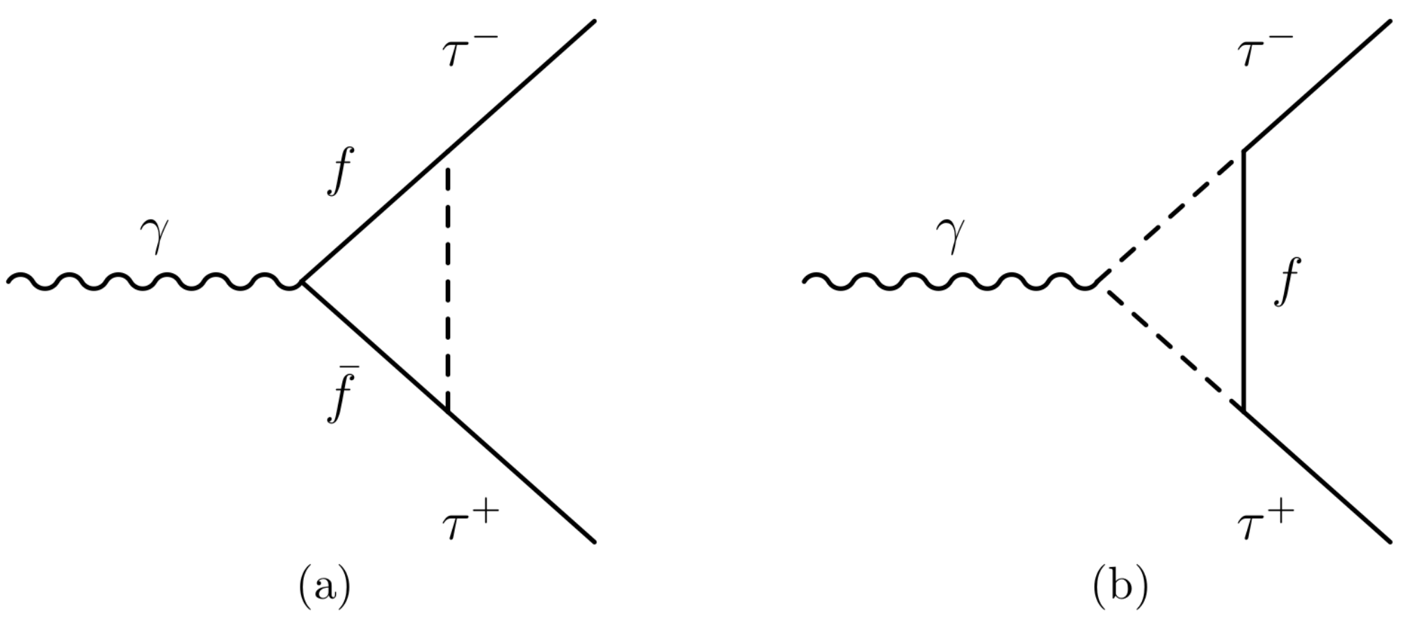
Here we identify with the Higgs boson and assume that and are heavier than . The exchange of the induces a EDM at one loop shown by the diagram Fig. 3a. With the convention of Eq. (2) we get77 7 The real and imaginary parts of the EDM form factor of a fermion were computed for a class of 2HDM including the type-II model in [41] and evaluated for the top quark.
| (99) |
| (100) |
where and is the mass of . The functions and denote the standard scalar one-loop two-point and three-point functions [42]. For the EDM form factor (99) has both a real and an imaginary part.
However, apart from the upper bound (1) on the electron EDM existing constraints from experiments at the LHC preclude a EDM of order or larger in this model. A recent analysis of the decay of the 125 GeV Higgs boson to by the CMS experiment restricts the size of a potentially existing pseudoscalar coupling of to the lepton: at C.L. [43]. Searches for additional neutral Higgs bosons with decays to exclude Higgs-boson masses of about 400 GeV and below for a large range of Higgs coupling to leptons; see, for example, [44, 45] and references therein.
We exemplify the order of magnitude of that is compatible with these constraints by assuming the masses of the Higgs bosons and to be GeV and GeV, respectively. Moreover, we choose and the angles of the mixing matrix , in the parametrization of [40], to be , . The resulting real and imaginary parts of the EDM (99) are given in Table 9 for several c.m. energies in the energy range considered in this paper.
| [GeV] | 3.6 | 4 | 10.58 | 12 |
|---|---|---|---|---|
| 2.24 | 2.13 | 1.38 | 1.30 | |
| 0.13 | 0.38 | 0.77 | 0.78 |
By and large the order of magnitude of the EDM form factor listed in Table 9 is characteristic for a large class of Higgs models. Significantly larger values of and would be possible if, for instance, Higgs bosons exist with exclusive -violating couplings to the third generation of quarks and leptons, such that the stringent constraint (1) on the electron EDM can be evaded.
6.2 Spin-zero leptoquarks
Leptoquarks, whose interactions connect a lepton and a quark, occur naturally in unified models of strong and electroweak interactions. In recent years they have come again into the focus of numerous investigations in the context of possible explanations of semileptonic and meson decay and muon anomalies; see, for instance, [46, 47, 48, 49, 50] and references therein. Here we are interested in spin-zero leptoquarks with -violating Yukawa couplings. They can generate EDMs of the muon and tau lepton that are significantly larger than that of the electron,88 8 A recent analysis of the effects of spin-zero leptoquarks on the EDMs of leptons, quarks, and nucleons was made in [51]. as pointed out some time ago in [52, 24] (cf. also [53]).
We consider in the following two different spin-zero leptoquark models, namely the SM extended by a weak leptoquark doublet with quantum numbers (model I) and a SM extension by a weak singlet with quantum numbers (model II). The gauge-invariant interaction Lagrangians are [54]
| (101) |
| (102) |
Here , , , , where is a generation index. The label denotes charge conjugation. The matrix acts on the SU(2) indices. The electric charge (in units of ) of is . For the components of the doublet we have and The , and , denote complex matrices in flavor space. Usually the interactions (101) and (102) are defined in the weak basis and are rotated, after electroweak symmetry breaking, to the mass basis. We can choose a basis in which the Yukawa matrices of the up-type quark and of the charged-lepton couplings to the SM Higgs boson are already diagonal. Then only the down-type quark and neutrino fields must be rotated with their respective mixing matrices when one transforms to the mass basis. The interactions in (101) involving charged leptons and up-type quarks, with which we are concerned here, remain unaffected.
We assume that the off-diagonal elements of the matrices , and , in generation space are very small and can be neglected. Let us denote
| (103) |
and
| (104) |
If then the interaction Eq. (101) (Eq. (102)) generates a nonzero EDM at one loop. It is represented by Figs. 3 a) and 3 b) where the internal fermion and boson lines correspond to the top quark and the leptoquark in model I and to and in model II, respectively. The EDM form factor is given by [24]
| (105) |
where , is the mass of the top quark which provides the chirality flip, and in case of model I (II), where denotes either or . Moreover
| (106) | |||||
| (107) |
Here is the mass of in the case of model I (II). Because in the kinematic range that we consider here, the EDM form factor (105) is real.
In order to estimate the potential size of we choose the leptoquark masses TeV () which are compatible with the experimental bounds from LHC [55, 56] and the constraints from the anomalous magnetic moments of the electron and muon [49]. For comparison we evaluate (105) also for TeV and TeV. With GeV [1] we get from (105) the values listed in Table 10.
| [GeV] | 3.6 | 4 | 10.58 | 12 |
|---|---|---|---|---|
| Model I: | 14.44 | 14.44 | 14.45 | 14.45 |
| 7.89 | 7.89 | 7.89 | 7.89 | |
| 5.04 | 5.04 | 5.04 | 5.04 | |
| Model II: | 8.85 | 8.85 | 8.86 | 8.86 |
| 5.24 | 5.24 | 5.25 | 5.25 | |
| 3.51 | 3.51 | 3.51 | 3.51 |
The numbers in Table 10 show that for a given leptoquark mass the form factor is essentially flat in the kinematic range considered here. So far, the experimental bounds on the parameters , are not stringent. Using the experimental bound (1) and the numbers given in Table 10 for GeV and TeV, we get
| (108) |
If leptoquark couplings to the lepton and the quark are taken into account in (101) and (102) then develops also an imaginary part for . However, away from the charm threshold, the -quark contribution to is suppressed in magnitude by the factor as compared to the leading contribution (105), regardless of additional suppression due to small off-diagonal Yukawa couplings.
One may expect that the Yukawa couplings of the spin-zero leptoquarks are of the Higgs-boson type. Then the (diagonal) couplings of and in (101) and (102) will be proportional to the right-handed fermion involved. That is,
| (109) |
where and are mass scales that are expected to be larger than the electroweak symmetry breaking scale GeV. In this case the magnitude of will be smaller by a factor of at least than the numbers listed in Table 10.
6.3 Box contributions
The one-loop -matrix element of can receive in SM extensions also one-particle irreducible -violating box contributions that involve Lorentz structures such as . Here we argue that in the models considered in Sections 6.1 and 6.2 these contributions that are depicted in Fig. 4 can be neglected compared to those of the EDM form factors.
In the type-II 2HDM only diagram a) appears. From the Yukawa interaction (97) one obtains that this contribution is proportional to . Thus this contribution to the -matrix element of is negligible compared to that of the EDM form factor (100).
As to the spin-zero leptoquark models: If one considers interactions (101), (102) that are diagonal in generation space, then only diagram a) contributes with , and this contribution entails a suppression factor where is the mass of the quark. In the case of interactions that are nondiagonal in generation space, diagrams 4 a) and 4 b) contribute, but those contributions that involve leptoquark couplings between the electron and the and quark contain off-diagonal matrix elements or that are small due to experimental constraints (see, e.g., [49, 50]).
Thus we conclude that within the above SM extensions the -violating part of the one-loop -matrix element of is given to very good approximation by the contribution from the EDM form factor. In addition, we remark that the one-loop EDM form factors computed in Sections 6.1 and 6.2 are gauge invariant. Needless to say, the contribution of the electron EDM form factor to this matrix element is completely irrelevant.
7 Conclusions
The huge data samples of production and decay that will eventually be recorded at existing low-energy colliders will allow, among other investigations, the search for a electric dipole form factor with a precision that is significantly higher than existing bounds. We reconsidered the issue of using simple and optimal observables for such measurements. We discussed the general formalism of optimal observables and applied it to two -odd observables based on -odd -spin correlations and polarization asymmetries that are sensitive to the real and imaginary parts of , respectively. Special emphasis was put on the covariance of these observables. In our numerical analysis we computed the expectation values and covariances of the optimal observables for -pair production in collisions at the resonance with subsequent decays of to major leptonic or semihadronic modes. These results hold also for the continuum production of pairs at GeV. For the decays to two pions and three charged pions we took the full kinematic information of the hadronic system into account by incorporating the respective differential decay density matrices into the optimal observables. In this way the maximal -spin analyzing power is obtained also with these decay modes. Assuming that the Belle II experiment will eventually record and analyze events at GeV we found that with purely semihadronic decays 1 s.d. sensitivities and can be obtained with these optimal observables. For this is better than a factor of 5 and for better than a factor of 3 as the sensitivities attainable with the simple -odd observables that we analyzed, too. Including events where one (or both) leptons decay leptonically does not lead to a significant increase in sensitivity to and . These results were obtained without cuts. We analyzed also the sensitivity of the optimal observables to and in the purely semihadronic decay channels by applying cuts on the final-state pions. Assuming an integrated luminosity of 50 ab-1, which corresponds to the above number of events in the case of no cuts, we obtained and . That is, the 1 s.d. sensitivities decrease only slightly.
Furthermore, we discussed a few SM extensions with nonstandard violation that predict an nonzero EDM already at one-loop order. The tight experimental upper bound on the electron EDM, experimental results from the LHC on the nature of the 125 GeV Higgs boson, and bounds on the mass and couplings of new particles severely constrain the potential magnitude of . Within the type-II 2HDM, which we consider in this context to be exemplary for a large class of two-Higgs doublet extensions of the SM, the EDM form factor turns out to be too small to be detected in the foreseeable future. However, in scalar leptoquark extensions of the SM is still possible in the energy range considered in this paper. In any case, future EDM measurements with the Belle II and also the BES III experiment using optimal observables will provide significant information about new sources of violation.
Acknowledgments
The authors thank M. Diehl, R. Karl, F. M. Krinner, F. Nerling, A. Rostomyan, and A. Szczurek for discussions and correspondence, and C. Ewerz for help with one figure. The work of L.C. was supported by the Deutsche Forschungsgemeinschaft under Grant No. 396021762-TRR 257.
Appendix A decay density matrices
Here we list the density matrices that describe several major decays of polarized . Most of them given below are used in section 5. The kinematic variables in this appendix are defined in the respective rest frame unless stated otherwise. The decay density matrices are computed in the Standard Model; potential -violating effects in decays are not taken into account.
First we consider decays into one charged prong, with particle multiplicity . The charged particle acts as the spin analyzer. Assuming invariance in the decays of we have in the rest frame:
| (110) |
where is the transform of and . If denotes a lepton, we have ; for meson, is the product of the intrinsic parity and charge-parity quantum numbers of . Thus, for a pion ( meson) we get . Equation (110) implies for the decay density matrices
| (111) |
The respective decay density matrix defined in (26) and (27) is of the form
| (112) |
where is the energy of and . In (112) the symbol l denotes the two-dimensional unit matrix and is the vector of Pauli matrices. The function determines the energy spectrum of while encodes the -spin analyzing power of the charged prong. Equation (112) is used in the calculations of Sec. 5. If the right-hand side of (112) is integrated over , it takes, due to the normalization convention (27), the form
| (113) |
where is a measure of the spin-analyzing power of .
Next we list the spectral functions and of several decay density matrices (112). The functions have dimension 1/energy while the functions are dimensionless.
The decay
In the leptonic decays the mass of can be neglected. (Here and below the symbol denotes a neutrino or antineutrino, depending on the case.) Using , where is defined in the rest frame, one has [57]
| (114) |
with . Integrating over the charged lepton energy in (112) yields (113) with the -spin analyzing power
| (115) |
The value of can be increased by a suitable cut on .
The decay
In the two-body decay the energy in the rest frame is fixed and the functions and are given by [57]:
| (116) |
Here the -spin analyzing power is maximal,
| (117) |
The decay
If the four-momentum of the intermediate meson can be determined in the decay by measuring the energies and momenta of both and , the meson can be used as -spin analyzer. It is well known that in the two-body decay of a polarized to a transversely or longitudinally polarized spin-1 meson and the -spin analyzing power of the meson is maximal [58]. However, the polarization of the vector meson cannot be determined event by event. Summing over the polarizations of the meson and treating it as an on-shell particle, one obtains decay density matrices of the form (112) with the spectral functions [57, 58]
| (118) |
Using we obtain
| (119) |
We use this two-body decay mode with (112) and (118) in our analysis of the simple observables in Sec. 5.
The decay
The differential rate of the decay of polarized leptons to a charged and neutral pion via a meson was calculated in [57] in the on-shell approximation for the intermediate meson. A more elaborate description of this decay mode takes the and resonances and their finite widths as intermediate states into account [59, 60, 61]. We use the matrix element of [59, 60] for the decay chain . Exact isospin invariance is assumed. In the rest frame we obtain for the decay density matrix that is differential in the pion momenta:
| (120) |
where and
| (121) |
Here and denote the Fermi constant and the Cabibbo-Kobayashi-Maskawa matrix element, respectively. The terms in the squared matrix element are
| (122) | |||||
| (123) |
where , in the rest frame, , and .
The phase-space measure can be parametrized as follows:
| (124) |
where is the solid angle element of , i.e. of , in the rest frame and is the solid angle element of the charged pion in the rest frame of . Moreover,
| (125) |
The form factor in (121) can be parametrized by [59]
| (126) |
where
| (127) |
The label () refers to the () resonance and is a tuning parameter (see below).
We use for the energy-dependent off-shell widths of the and that are needed in (127):
| (128) |
where
and is given by the same formula with label . A value for the on-shell width and , respectively, is given in (129).
We use the following input values for the computations of the optimal observables in Sec. 5:
| (129) |
With this input, agreement with the experimental width is obtained when the tuning parameter in Eq. (126) is chosen to be
| (130) |
The differential decay density matrix for the charge-conjugate decay
is of the same form as (120) with the squared matrix element
| (131) |
One may also determine the -spin analyzing power of the “resonance” in the decay mode by computing the following decay density matrix:
| (132) |
where and . The spectral functions and are shown in Fig. 5. Integrating the right-hand side of (132) over the decay density matrix takes the form (113) with and We get for :
| (133) |
Comparison with (119) shows that taking into account the finite widths of the intermediate resonances and the whole kinematic range of leads to a slightly smaller -spin analyzing power. Nevertheless, we will use the value (119) in the computation of the expectation values of the simple observables in Sec. 5.
For completeness we determine also the -spin analyzing power of the charged pion in . The respective 1-prong decay density matrix is given by
| (134) |
where and . The spectral functions and are shown in Fig. 6. Integrating the right-hand side of (134) over the decay density matrix takes the form (113) with and . We get for the -spin analyzing power of the charged pion99 9 This decay mode was analyzed in [9] using only the intermediate in the narrow-width approximation.
| (135) |
Figure 6 shows that negative and positive contributions cancel to a large extent when is integrated over the whole kinematic range, leading to the small value (135). The value of can be enhanced by a suitable cut on . We do not use (134) in our analysis of Sec. 5.
The decay
The decay mode to three charged prongs proceeds mainly via an intermediate resonance. If one approximates the decay mode by decay to an on-shell , the -spin analyzing power of this resonance would be maximal, as stated above, if the polarization states can be separated efficiently [58, 34]. If one sums over the polarizations the decay density matrix is of the form (112) and (118) with the label . The mass is not precisely determined but, in any case, the -spin analyzing power of this resonance is poor in the on-shell approximation. Using (118) (with ) with the value given by the Particle Data Group [1] one obtains .
However, maximal sensitivity to the polarization can be obtained with the decay mode if the full decay dynamics is exploited and the energies and momenta of the three pions are measured. We use the matrix element given in [59] (cf. also [60, 61]) where this decay is described by the decay chain with off-shell intermediate resonances. Exact isospin invariance is assumed.1010 10 The decay was analyzed in [62] within the resonance chiral theory using an elaborate description of the off-shell width. We obtain for the differential decay density matrix in the rest frame with the normalization conventions (3) and (32):
| (136) |
where and the phase-space measure is given in the recursive phase-space parametrization by
| (137) |
Here , and is the solid angle element of , i.e. , in the rest frame, is the solid angle element of in the rest frame of , and is the solid angle element of in the rest frame of , i.e., the zero-momentum frame of . Note that the statistics factor for two identical particles in the final state is compensated here by the normalization convention (32). The squared matrix element is given by
| (138) |
where
| (139) | |||||
| (140) | |||||
and , , ,
| (141) |
and , and we use the convention . Moreover,
| (142) |
where and . The function is given by [59]:
| (143) |
where is the pion decay constant (in the convention GeV) and denotes the Breit-Wigner enhancement factor of the meson:
| (144) |
We use as a model for the energy-dependent off-shell width of the meson:
| (145) |
where is the on-shell width (see below) and the function is given in Eq. (3.16) of Ref. [59]. Moreover, the pion “form factor” is given by the formulas (126) – (128) above where now the tuning parameter is to be replaced by that will be determined below.
The differential decay density matrix for the charge-conjugate decay
is of the same form as Eqs. (136) with the squared matrix element
| (146) |
To the best of our knowledge the differential density matrix (136) – (140) was so far not given in this explicit form in the literature.
For our computation of the expectation values of the optimal observables in Sec. 5 we use the above formulas with the input values (129) and
| (147) |
It remains to fix the tuning parameter . Using the above squared matrix element and input parameters we find agreement with the experimental width when the tuning parameter is chosen to be
| (148) |
The decay
For completeness we discuss here also this decay mode, although we do not use it in the analysis of Sec. 5. Assuming exact isospin invariance the differential decay density matrices for derived in the previous subsection can be used also for these decay modes. Using the above input parameters with the exception , agreement with the experimental width is obtained with the following value of the tuning parameter, here denoted by :
| (149) |
Moreover, the -spin analyzing power of the charged pion in this decay mode is also of interest. The 1-prong decay density matrix for , normalized to the charged particle multiplicity , is given by
| (150) |
where and . The spectral functions and are shown in Fig. 7. Integrating the right-hand side of (150) over the decay density matrix takes the form (113) with and We get for the -spin analyzing power of the charged pion:1111 11 A simpler description of this decay mode was used in [9] and the value was obtained.
| (151) |
This number is rather small because has both negative and positive contributions that cancel to a large extent when integrated over . The analyzing power can be enhanced by a suitable cut on .
Appendix B Expectation values and covariances of -odd observables
In this appendix we discuss general properties of expectation values and covariances of the -odd observables introduced in Sec. 4 and computed in Sec. 5. We treat first case i) of Sec. 3 where only one charged particle is measured from and decays, respectively. The differential cross section of the two-particle inclusive reaction (28) and (29) as used in this paper is given by (3):
| (152) | |||||
where we have used in (3) the momenta of the charged particles and and the corresponding phase-space measures in the respective and rest frame. The one-particle inclusive decay density matrices in the rest frames are given in (112). We recall the relation between the respective rest-frame momenta and and the momenta and in the c.m. frame. With the Lorentz boost
| (153) |
where is the three-momentum of in the c.m. frame, we have
| (154) |
Next we decompose (152) according to (51) and (52), neglecting terms quadratic in . Here our phase-space variables are
| (155) |
and the measure is
| (156) |
We get
| (157) |
where, using (112),
| (158) | |||||
The quantities and are obtained from (158) by the replacements
| (159) |
We can now perform the traces in (158). With (3) we see that this amounts to make the following replacements in (38) – (40):
| l | |||||
| (160) |
Next, we consider the transformation
| (161) |
which, using (154), implies
| (162) |
and vice versa. These transformations correspond to the naive ‘‘time reversal’’ transformation1212 12 One may also transform , but this is irrelevant here. referred to in Sec. 3. Inspection of , , and , i.e., of Eqs. (38) – (40) with the replacements (B), shows that applying (162) we have
| (163) |
We turn to the simple and optimal observables of Sec. 4. We assume integration over the whole phase space or, if cuts are applied, we assume the cuts to be -symmetric. In addition we assume the cuts to be invariant under (161). The tensors and of (44) and (45) are odd whereas and of (46) and (47) are even under the transformation (161).
Let us first consider the case . The properties of the observables and imply
| (164) |
Moreover, turning to the covariance matrix of one of the and one of the variables, the transformation (161) implies
| (165) |
and likewise for the other correlations. That is, the covariance matrix of the variables is diagonal.
The optimal observables are in the case :
| (166) |
The transformation properties of these observables imply
| (167) |
and applying the transformation (161) it follows that
| (168) |
Thus, the covariance matrix is diagonal in this case:
| (169) |
Next we turn to the case . As this final state is no longer -symmetric, the transformation properties of the observables are no longer of immediate use. Let us first consider the simple observables, for instance, and . Applying the transformation (161) we get
| (170) |
The transformation (161) implies also that expectation values of the form (165) vanish in the nondiagonal case. As to the SM expectation value
| (171) |
there is, however, in the case no symmetry argument implying that it vanishes, too. Therefore, one should use in this case in general the observables
| (172) |
From the property of one gets, of course,
| (173) |
Thus, the respective quantity to probe for violation is (49):
| (174) |
But the corresponding variance in the SM, for instance of the components, has to be calculated in general as
| (175) |
The above statements apply, of course, also to . Yet in our analysis where we use the SM matrix element of the form (158) and integrate over the whole phase space we find that (171) vanishes within our numerical uncertainties of order . This holds also for the respective expectation values of .
The optimal observables are in the case (cf. (86)):
| (176) |
where and are odd and even under the transformation (162), respectively; see (163). Therefore, we have
| (177) |
For analyzing we perform in , Eq. (157), the variable transformation
| (178) |
The term remains invariant, while change sign; see (38) – (40) and (158), (159). Thus
| (179) |
if one integrates over the whole angular range of or over a range that is symmetric with respect to (178). Beyond the one-photon approximation will in general be nonzero. Therefore, one should use in general (cf. (56)):
| (180) |
In our case here the transformations (162) and (178) imply that the covariance matrix is still diagonal and is given by
| (181) |
This covariance matrix is then used in (75) and (77) for the estimators and their covariance matrix .
We come now to the final states of case ii) of Sec. 3 to which we apply the optimal observables. The channels where is involved require a more detailed discussion. In our models for the hadronic decays outlined in Appendix A the squared matrix element of this decay mode given in (138) – (140) differs from the respective squared matrix element of and those of the one-particle inclusive decays in that it contains contributions from absorptive parts caused by the finite widths of the intermediate resonances. This implies that a transformation can no longer be used to discriminate between the optimal observables and . In order to see this explicitly let us for definiteness consider the case where decays to three observed pions (labeled by the symbol ), while in the decay of only one charged particle is measured (label ). The differential cross section is obtained by inserting the respective decay density matrices into (3), taking into account (3) – (33). Using (138) the matrix element is obtained from (158), up to an overall factor, by replacing
| (182) |
The matrix elements and are obtained in the same fashion. Inspection of the functions and shows that neither has a definite behavior under the following transformation that is analogous to (162):
| (183) |
The dispersive terms in and are even under (183) whereas the absorptive terms are odd. Therefore, the matrix elements , , and do not have a definite transformation behavior under (183), too. Hence we expect that
| (184) |
Thus, the covariance matrix can have nondiagonal elements that are nonvanishing. On the other hand, applying the transformation (178), , to and to shows that the first term remains invariant while the two others change sign. Therefore, with our matrix elements we have
| (185) |
Beyond the one-photon approximation (185) will no longer hold. Thus when -pair decays to final states , , and are considered, one should in general apply – especially in experimental analyses – the full formalism of the optimal observable method as explained in Sec. 4. The nondiagonal elements of the respective covariance matrix of the optimal observables computed with the matrix elements for -pair production and decay used in this paper at GeV are very small and can be neglected in view of our numerical uncertainties; see Sec. 5.
At last a remark that applies if the full formalism of Sec. 4 has to be used. Suppose the parameters and have been measured in decay channels. Let us denote the results for their mean values in the channel by
| (186) |
and for the respective covariance matrix by . Furthermore, we assume these measurements to be independent, i.e., uncorrelated. We define the matrix
| (187) |
and the overall mean
| (188) |
The covariance matrix is then given by . That is, the 1 s.d. error ellipse for the mean values (188) in the plane is given by
| (189) |
References
- [1] P. A. Zyla et al. [Particle Data Group], “Review of Particle Physics,” PTEP 2020, no.8, 083C01 (2020) doi:10.1093/ptep/ptaa104
- [2] V. Andreev et al. [ACME], “Improved limit on the electric dipole moment of the electron,” Nature 562, no.7727, 355-360 (2018) doi:10.1038/s41586-018-0599-8
- [3] G. W. Bennett et al. [Muon (g-2)], “An Improved Limit on the Muon Electric Dipole Moment,” Phys. Rev. D 80, 052008 (2009) doi:10.1103/PhysRevD.80.052008 [arXiv:0811.1207 [hep-ex]].
- [4] K. Inami et al. [Belle], “Search for the electric dipole moment of the tau lepton,” Phys. Lett. B 551, 16-26 (2003) doi:10.1016/S0370-2693(02)02984-2 [arXiv:hep-ex/0210066 [hep-ex]].
- [5] W. Bernreuther, U. Löw, J. P. Ma and O. Nachtmann, “CP Violation and Z Boson Decays,” Z. Phys. C 43, 117 (1989) doi:10.1007/BF02430617
- [6] W. Bernreuther and O. Nachtmann, “CP Violating Correlations in Electron Positron Annihilation Into Leptons,” Phys. Rev. Lett. 63, 2787 (1989), Phys.Rev.Lett. 64 (1990) 1072 (erratum) doi:10.1103/PhysRevLett.63.2787
- [7] J. G. Körner, J. P. Ma, R. Münch, O. Nachtmann and R. Schöpf, “CP Violating Correlations in the Reaction Hadrons,” Z. Phys. C 49, 447-458 (1991) doi:10.1007/BF01549698
- [8] W. Bernreuther, G. W. Botz, O. Nachtmann and P. Overmann, “CP violating effects in Z decays to tau leptons,” Z. Phys. C 52, 567-574 (1991) doi:10.1007/BF01562330
- [9] W. Bernreuther, O. Nachtmann and P. Overmann, “The CP violating electric and weak dipole moments of the tau lepton from threshold to 500-GeV,” Phys. Rev. D 48, 78-88 (1993) doi:10.1103/PhysRevD.48.78
- [10] H. Albrecht et al. [ARGUS], “A Search for the electric dipole moment of the tau lepton,” Phys. Lett. B 485, 37-44 (2000) doi:10.1016/S0370-2693(00)00630-4 [arXiv:hep-ex/0004031 [hep-ex]].
- [11] A. Stahl, “Physics with tau leptons,” Springer Tracts Mod. Phys. 160, 1-316 (2000) doi:10.1007/BFb0109630
- [12] W. Lohmann, “Electromagnetic and weak moments of the tau-lepton,” Nucl. Phys. B Proc. Suppl. 144, 122-127 (2005) doi:10.1016/j.nuclphysbps.2005.02.017 [arXiv:hep-ex/0501065 [hep-ex]].
- [13] J. Bernabeu, G. A. Gonzalez-Sprinberg and J. Vidal, “CP violation and electric-dipole-moment at low energy tau production with polarized electrons,” Nucl. Phys. B 763, 283-292 (2007) doi:10.1016/j.nuclphysb.2006.11.023 [arXiv:hep-ph/0610135 [hep-ph]].
- [14] J. Bernabeu, G. A. Gonzalez-Sprinberg, J. Papavassiliou and J. Vidal, “Tau anomalous magnetic moment form-factor at super B/flavor factories,” Nucl. Phys. B 790, 160-174 (2008) doi:10.1016/j.nuclphysb.2007.09.001 [arXiv:0707.2496 [hep-ph]].
- [15]
S. Eidelman, D. Epifanov, M. Fael, L. Mercolli and M. Passera,
“ dipole moments via radiative leptonic decays,” JHEP 03, 140 (2016) doi:10.1007/JHEP03(2016)140 [arXiv:1601.07987 [hep-ph]]. - [16] X. Chen and Y. Wu, “Search for the Electric Dipole Moment and anomalous magnetic moment of the tau lepton at tau factories,” JHEP 10, 089 (2019) doi:10.1007/JHEP10(2019)089 [arXiv:1803.00501 [hep-ph]].
- [17] M. Dyndal, M. Klusek-Gawenda, M. Schott and A. Szczurek, “Anomalous electromagnetic moments of lepton in reaction in Pb+Pb collisions at the LHC,” [arXiv:2002.05503 [hep-ph]].
- [18] T. Abe et al. [Belle-II], “Belle II Technical Design Report,” [arXiv:1011.0352 [physics.ins-det]].
- [19] E. Kou et al. [Belle-II], “The Belle II Physics Book,” PTEP 2019, no.12, 123C01 (2019) [erratum: PTEP 2020, no.2, 029201 (2020)] doi:10.1093/ptep/ptz106 [arXiv:1808.10567 [hep-ex]].
- [20] M. Ablikim et al. [BESIII], “Future Physics Programme of BES III,” Chin. Phys. C 44, no.4, 040001 (2020) doi:10.1088/1674-1137/44/4/040001 [arXiv:1912.05983 [hep-ex]].
- [21] D. Atwood and A. Soni, “Analysis for magnetic moment and electric dipole moment form-factors of the top quark via ,” Phys. Rev. D 45, 2405-2413 (1992) doi:10.1103/PhysRevD.45.2405
- [22] M. Davier, L. Duflot, F. Le Diberder and A. Rouge, “The Optimal method for the measurement of tau polarization,” Phys. Lett. B 306, 411-417 (1993) doi:10.1016/0370-2693(93)90101-M
- [23] M. Diehl and O. Nachtmann, “Optimal observables for the measurement of three gauge boson couplings in ,” Z. Phys. C 62, 397-412 (1994) doi:10.1007/BF01555899
- [24] W. Bernreuther, A. Brandenburg and P. Overmann, “CP violation beyond the standard model and tau pair production in e+ e- collisions,” Phys. Lett. B 391, 413-419 (1997) [erratum: Phys. Lett. B 412, 425-425 (1997)] doi:10.1016/S0370-2693(96)01501-8 [arXiv:hep-ph/9608364 [hep-ph]].
- [25] J. D. Bjorken and S. D. Drell, “Relativistic quantum fields,” Mc-Graw Hill, New York (1965).
- [26] S. Banerjee, B. Pietrzyk, J. M. Roney and Z. Was, “Tau and muon pair production cross-sections in electron-positron annihilations at GeV,” Phys. Rev. D 77, 054012 (2008) doi:10.1103/PhysRevD.77.054012 [arXiv:0706.3235 [hep-ph]].
- [27] Ia. B. Zel’dovich, “Electromagnetic Interaction with Parity Violation,” Sov. Phys. JETP 6, 1184 (1958)
- [28] V. V. Flambaum and I. B. Khriplovich, “ Odd Nuclear Forces as a Source of Parity Nonconservation in Atoms,” Sov. Phys. JETP 52, 835 (1980), IYF-80-136.
- [29] V. V. Flambaum, I. B. Khriplovich and O. P. Sushkov, “On the Possibility to Study Odd and Odd Nuclear Forces in Atomic and Molecular Experiments,” Sov. Phys. JETP 60, 873 (1984), IYF-84-85.
- [30] V. V. Flambaum, I. B. Khriplovich and O. P. Sushkov, “Nuclear Anapole Moments,” Phys. Lett. B 146, 367-369 (1984) doi:10.1016/0370-2693(84)90140-0
- [31] W. Buchmüller and D. Wyler, “Effective Lagrangian Analysis of New Interactions and Flavor Conservation,” Nucl. Phys. B 268, 621-653 (1986) doi:10.1016/0550-3213(86)90262-2
- [32] W. Bernreuther and O. Nachtmann, “A Note on CP odd and T odd observables at colliders,” Phys. Lett. B 268, 424-428 (1991) doi:10.1016/0370-2693(91)91601-Q
- [33] O. Nachtmann, “Elementary Particle Physics: Concepts and Phenomena,” Berlin, Springer (1990).
- [34] A. Rougé, “Polarization observables in the 3 pi neutrino decay mode,” Z. Phys. C 48, 75-78 (1990) doi:10.1007/BF01565607
- [35] J. H. Kühn, “Tau polarimetry with multimeson states,” Phys. Rev. D 52, 3128-3129 (1995) doi:10.1103/PhysRevD.52.3128 [arXiv:hep-ph/9505303 [hep-ph]].
- [36] J. H. Kühn, “Tau kinematics from impact parameters,” Phys. Lett. B 313, 458-460 (1993) doi:10.1016/0370-2693(93)90019-E [arXiv:hep-ph/9307269 [hep-ph]].
- [37] M. Pospelov and A. Ritz, “CKM benchmarks for electron electric dipole moment experiments,” Phys. Rev. D 89, no.5, 056006 (2014) doi:10.1103/PhysRevD.89.056006 [arXiv:1311.5537 [hep-ph]].
- [38] Y. Yamaguchi and N. Yamanaka, “Large long-distance contributions to the electric dipole moments of charged leptons in the standard model,” Phys. Rev. Lett. 125, 241802 (2020) doi:10.1103/PhysRevLett.125.241802 [arXiv:2003.08195 [hep-ph]].
- [39] S. M. Barr and A. Zee, “Electric Dipole Moment of the Electron and of the Neutron,” Phys. Rev. Lett. 65, 21-24 (1990) [erratum: Phys. Rev. Lett. 65, 2920 (1990)] doi:10.1103/PhysRevLett.65.21
- [40] W. Bernreuther, P. Galler, C. Mellein, Z. G. Si and P. Uwer, “Production of heavy Higgs bosons and decay into top quarks at the LHC,” Phys. Rev. D 93, no.3, 034032 (2016) doi:10.1103/PhysRevD.93.034032 [arXiv:1511.05584 [hep-ph]].
- [41] W. Bernreuther, T. Schröder and T. N. Pham, “CP violating dipole form-factors in ,” Phys. Lett. B 279, 389-396 (1992) doi:10.1016/0370-2693(92)90410-6
- [42] G. ’t Hooft and M. J. G. Veltman, “Scalar One Loop Integrals,” Nucl. Phys. B 153, 365-401 (1979) doi:10.1016/0550-3213(79)90605-9
- [43] [CMS Physics Analysis Summary], “Analysis of the CP structure of the Yukawa coupling between the Higgs boson and leptons in proton-proton collisions at ,” CMS-PAS-HIG-20-006.
- [44] C. Caputo [CMS and ATLAS], “Searches for additional Higgs bosons decaying to tau leptons at the LHC,” SciPost Phys. Proc. 1, 022 (2019) doi:10.21468/SciPostPhysProc.1.022
- [45] G. Aad et al. [ATLAS], “Search for heavy Higgs bosons decaying into two tau leptons with the ATLAS detector using collisions at TeV,” Phys. Rev. Lett. 125, no.5, 051801 (2020) doi:10.1103/PhysRevLett.125.051801 [arXiv:2002.12223 [hep-ex]].
- [46] M. Bauer and M. Neubert, “Minimal Leptoquark Explanation for the R, RK, and Anomalies,” Phys. Rev. Lett. 116, no.14, 141802 (2016) doi:10.1103/PhysRevLett.116.141802 [arXiv:1511.01900 [hep-ph]].
- [47] E. Coluccio Leskow, G. D’Ambrosio, A. Crivellin and D. Müller, “, lepton flavor violation, and decays with leptoquarks: Correlations and future prospects,” Phys. Rev. D 95, no.5, 055018 (2017) doi:10.1103/PhysRevD.95.055018 [arXiv:1612.06858 [hep-ph]].
- [48] A. Crivellin, M. Hoferichter and P. Schmidt-Wellenburg, “Combined explanations of and implications for a large muon EDM,” Phys. Rev. D 98, no.11, 113002 (2018) doi:10.1103/PhysRevD.98.113002 [arXiv:1807.11484 [hep-ph]].
- [49] I. Bigaran and R. R. Volkas, “Getting chirality right: single scalar leptoquark solution/s to the puzzle,” [arXiv:2002.12544 [hep-ph]].
- [50] A. Crivellin, C. Greub, D. Müller and F. Saturnino, “Scalar Leptoquarks in Leptonic Processes,” [arXiv:2010.06593 [hep-ph]].
- [51] W. Dekens, J. de Vries, M. Jung and K. K. Vos, “The phenomenology of electric dipole moments in models of scalar leptoquarks,” JHEP 01, 069 (2019) doi:10.1007/JHEP01(2019)069 [arXiv:1809.09114 [hep-ph]].
- [52] W. Bernreuther, “The Electric dipole moment of the muon,” Z. Phys. C 56, S97-S100 (1992) HD-THEP-91-37.
- [53] P. Poulose and S. D. Rindani, “CP violating dipole form-factors of the top quark and lepton in scalar leptoquark models,” Pramana 51, 387-403 (1998) doi:10.1007/BF02828932 [arXiv:hep-ph/9708332 [hep-ph]].
- [54] W. Buchmüller, R. Rückl and D. Wyler, “Leptoquarks in Lepton - Quark Collisions,” Phys. Lett. B 191, 442-448 (1987) [erratum: Phys. Lett. B 448, 320-320 (1999)] doi:10.1016/0370-2693(87)90637-X
- [55] A. M. Sirunyan et al. [CMS], “Search for leptoquarks coupled to third-generation quarks in proton-proton collisions at 13 TeV,” Phys. Rev. Lett. 121, no.24, 241802 (2018) doi:10.1103/PhysRevLett.121.241802 [arXiv:1809.05558 [hep-ex]].
- [56] M. Aaboud et al. [ATLAS], “Searches for third-generation scalar leptoquarks in = 13 TeV pp collisions with the ATLAS detector,” JHEP 06, 144 (2019) doi:10.1007/JHEP06(2019)144 [arXiv:1902.08103 [hep-ex]].
- [57] Y. -S. Tsai, “Decay Correlations of Heavy Leptons in Lepton+ Lepton-,” Phys. Rev. D4, 2821 (1971) [erratum: Phys. Rev. D 13, 771 (1976)] doi:10.1103/PhysRevD.13.771
- [58] K. Hagiwara, A. D. Martin and D. Zeppenfeld, “Tau Polarization Measurements at LEP and SLC,” Phys. Lett. B 235, 198-202 (1990) doi:10.1016/0370-2693(90)90120-U
- [59] J. H. Kühn and A. Santamaria, “Tau decays to pions,” Z. Phys. C 48, 445-452 (1990) doi:10.1007/BF01572024
- [60] S. Jadach, J. H. Kühn and Z. Was, “TAUOLA: A Library of Monte Carlo programs to simulate decays of polarized tau leptons,” Comput. Phys. Commun. 64, 275-299 (1991) doi:10.1016/0010-4655(91)90038-M
- [61] K. Hagiwara, T. Li, K. Mawatari and J. Nakamura, “TauDecay: a library to simulate polarized tau decays via FeynRules and MadGraph5,” Eur. Phys. J. C 73, 2489 (2013) doi:10.1140/epjc/s10052-013-2489-4 [arXiv:1212.6247 [hep-ph]].
- [62] D. G. Dumm, P. Roig, A. Pich and J. Portoles, “ decays and the off-shell width revisited,” Phys. Lett. B 685, 158-164 (2010) doi:10.1016/j.physletb.2010.01.059 [arXiv:0911.4436 [hep-ph]].