Interpolation by multivariate polynomials in convex domainsThanks: Supported by the the Spanish Ministerio de Economía y Competividad (grant MTM2017-83499-P) and the Generalitat de Catalunya (grant 2017 SGR 358)

Jorge Antezana Address: Departamento de Matemática, Universidad Nacional de La Plata, and Instituto Argentino de Matemática “Alberto P. Calderón” (IAM-CONICET), Buenos Aires, Argentina Email address: antezana@mate.unlp.edu.ar , Jordi Marzo Address: Dept. Matemàtica i Informàtica, Universitat de Barcelona and BGSMath, Gran Via 585, 08007 Barcelona, Spain Email address: jmarzo@ub.edu and Joaquim Ortega-Cerdà Address: Dept. Matemàtica i Informàtica, Universitat de Barcelona and BGSMath, Gran Via 585, 08007 Barcelona, Spain Email address: jortega@ub.edu

Date: August 11, 2026

Abstract.

Let $\Omega$ be a convex open set in $\mathbb{R}^{n}$ and let $\Lambda_{k}$ be a finite subset of $\Omega$ . We find necessary geometric conditions for $\Lambda_{k}$ to be interpolating for the space of multivariate polynomials of degree at most $k$ . Our results are asymptotic in $k$ . The density conditions obtained match precisely the necessary geometric conditions that sampling sets are known to satisfy and they are expressed in terms of the equilibrium potential of the convex set. Moreover we prove that in the particular case of the unit ball, for $k$ large enough, there is no family of orthogonal reproducing kernels in the space of polynomials of degree at most $k$ .

1. Introduction

Given a measure $\mu$ in $\mathbb{R}^{n}$ we consider the space $\mathcal{P}_{k}$ of polynomials of total degree at most $k$ in $n$ -variables endowed with the natural scalar product in $L^{2}(\mu)$ . We assume that $L^{2}(\mu)$ is a norm for $\mathcal{P}_{k}$ , i.e. the support of $\mu$ is not contained in the zero set of any $p\in\mathcal{P}_{k}$ , $p\neq 0$ . In this case the point evaluation at any given point $x\in\mathbb{R}^{n}$ is a bounded linear functional and $(\mathcal{P}_{k},L^{2}(\mu))$ becomes a reproducing kernel Hilbert space, i.e for any $x\in\mathbb{R}^{n}$ , there is a unique function $K_{k}(\mu,x,\cdot)\in\mathcal{P}_{k}$ such that

p(x)=\langle p,K_{k}(\mu,x,\cdot)\rangle=\int p(y)K_{k}(\mu,x,y)\,d\mu(y).

Given a point $x\in\mathbb{R}^{n}$ the normalized reproducing kernel is denoted by $\kappa_{k,y}$ , i.e.

\kappa_{k,y}(\mu,x)=\frac{K_{k}(\mu,x,y)}{\|K_{k}(\mu,x,\cdot)\|_{L^{2}(\mu)}}=\frac{K_{k}(\mu,x,y)}{\sqrt{K_{k}(\mu,x,x)}}.

We will denote by $\beta_{k}(\mu,x)$ the value of the reproducing kernel in the diagonal

\beta_{k}(\mu,x)=K_{k}(\mu,x,x).

The function $1/\beta_{k}(\mu,x)$ is the so called Christoffel function. For brevity we may omit sometimes the dependence on $\mu$ .

Following Shapiro and Shields in [15] we define sampling and interpolating sets:

Definition 1.

A sequence $\Lambda=\{\Lambda_{k}\}$ of finite sets of points on $\mathbb{R}^{n}$ is said to be interpolating for $(\mathcal{P}_{k},L^{2}(\mu))$ if the associated family of normalized reproducing kernels at the points $\lambda\in\Lambda_{k}$ , i.e. $\kappa_{k,\lambda},$ is a Riesz sequence in the Hilbert space $\mathcal{P}_{k}$ , uniformly in $k$ , i.e there is a constant $C>0$ independent of $k$ such that for any linear combination of the normalized reproducing kernels we have:

(1.1)

\frac{1}{C}\sum_{\lambda\in\Lambda_{k}}|c_{\lambda}|^{2}\leq\bigl\|\sum_{\lambda\in\Lambda_{k}}c_{\lambda}\kappa_{k,\lambda}\bigr\|^{2}\leq C\sum_{\lambda\in\Lambda_{k}}|c_{\lambda}|^{2},\quad\forall\{c_{\lambda}\}_{\lambda\in\Lambda_{k}}.

The definition above is usually decoupled in two separate conditions. The left hand side inequality in (1.1) is usually called the Riesz-Fischer property for the reproducing kernels and it is equivalent to the fact that the following moment problem is solvable: for arbitrary values $\{v_{\lambda}\}_{\lambda_{\in}\Lambda_{k}}$ there exists a polynomial $p\in\mathcal{P}_{k}$ such that $p(\lambda)/\sqrt{\beta_{k}(\lambda)}=\langle p,\kappa_{k,\lambda}\rangle=v_{\lambda}$ for all $\lambda\in\Lambda_{k}$ and

\|p\|^{2}\leq C\sum_{\lambda\in\Lambda_{k}}|v_{\lambda}|^{2}=\sum_{\lambda\in\Lambda_{k}}\frac{|p(\lambda)|^{2}}{\beta_{k}(\lambda)}.

This is the reason $\Lambda$ is called an interpolating family.

The right hand side inequality in (1.1) is called the Bessel property for the normalized reproducing kernels $\{\kappa_{k,\lambda}\}_{\lambda\in\Lambda_{k}}$ . The Bessel property is equivalent to have

(1.2)

\sum_{\lambda\in\Lambda_{k}}\frac{|p(\lambda)|^{2}}{\beta_{k}(\lambda)}\leq C\|p\|^{2}

for all $p\in\mathcal{P}_{k}.$ That is, if we denote $\mu_{k}:=\sum_{\lambda\in\Lambda_{k}}\frac{\delta_{\lambda}}{\beta_{k}(\lambda)}$ , we are requiring that the identity is a continuous embedding of $(\mathcal{P}_{k},L^{2}(\mu))$ into $(\mathcal{P}_{k},L^{2}(\mu_{k}))$ .

The notion of sampling play a similar but opposed role.

Definition 2.

A sequence $\Lambda=\{\Lambda_{k}\}$ of finite sets of points on $\mathbb{R}^{n}$ is said to be sampling or Marcinkiewicz-Zygmund for $(\mathcal{P}_{k},L^{2}(\mu))$ if the associated family of normalized reproducing kernels at the points $\lambda\in\Lambda_{k}$ , $\kappa_{k,\lambda}(x)$ is a frame in the Hilbert space $\mathcal{P}_{k}$ , uniformly in $k$ , i.e there is a constant $C>0$ independent of $k$ such that for any polynomial $p\in P_{k}$ :

(1.3)

\frac{1}{C}\sum_{\lambda\in\Lambda_{k}}|\langle p,\kappa_{k,\lambda}\rangle|^{2}\leq\|p\|^{2}\leq C\sum_{\lambda\in\Lambda_{k}}|\langle p,\kappa_{k,\lambda}\rangle|^{2},\quad\forall p\in\mathcal{P}_{k}.

Observe that the left hand side inequality in (1.3) is the Bessel condition mentioned above. If we were considering a single space of polynomials $\mathcal{P}_{k_{0}}$ then the notion of interpolating family amounts to say that the corresponding reproducing kernels are independent. On the other hand, the notion of sampling family corresponds to the reproducing kernels span the whole space $\mathcal{P}_{k_{0}}$ .

In this work we will restrict our attention to two classes of measures:

•

The first is $d\mu(x)=\chi_{\Omega}(x)dV(x)$ where $\Omega$ is a smooth bounded convex domain and $dV$ is the Lebesgue measure.
•

The second is of the form $d\mu(x)=(1-|x|^{2})^{a-1/2}\chi_{\mathbb{B}}(x)dV(x)$ where $a\geq 0$ and $\mathbb{B}$ is the unit ball $\mathbb{B}=\{x\in\mathbb{R}^{n}:|x|\leq 1\}$ .

In these two cases there are good explicit estimates for the size of the reproducing kernel on the diagonal $K_{k}(\mu,x,x),$ and therefore both notions, interpolation and sampling families, become more tangible. In [2] the authors obtained necessary geometric conditions for sampling families in bounded smooth convex sets with weights when the weights satisfy two technical conditions: Bernstein-Markov and moderate growth. These properties are both satisfied for the Lebesgue measure in a convex set. The case of interpolating families in convex sets was not considered, since there were several technical hurdles to apply the same technique.

Our aim in this paper is to fill this gap and obtain necessary geometric conditions for interpolating families in the two settings mentioned above. The geometric conditions that usually appear in this type of problem come into three flavours:

•

A separation condition. This is implied by the Riesz-Fischer condition i.e. the left hand side of (1.1). The fact that one should be able to interpolate the values one and zero implies that different points $\lambda,\lambda^{\prime}\in\Lambda_{k}$ with $\lambda\neq\lambda^{\prime}$ cannot be too close. The separation conditions in our settings are studied in Section 3.1.
•

A Carleson type condition. This is a condition that ensures the continuity of the embedding as in (1.2). A geometric characterization of the Carleson is given in Theorem 6 for convex domains and the Lebesgue measure, and in Theorem 7 for the ball and the measures $\mu_{a}$ .
•

A density condition. This is a global condition that usually follows from both the Bessel and the Riesz-Fischer condition. A density necessary condition for interpolating sequences is provided in Theorem 9 for convex sets endowed with the Lebesgue measure, and in Theorem 10 for the ball and the measures $\mu_{a}$ . Moreover, in this last setting we get an extension of the density results proved in [2] for sampling sequences.

Finally, a natural question is whether or not there exists a family $\{\Lambda_{k}\}$ that is both sampling and interpolating. To answer this question is very difficult in general [13]. A particular case is when $\{\kappa_{k,\lambda}\}_{\lambda\in\Lambda_{k}}$ form an orthonormal basis. In the last section we study the existence of orthonormal basis of reproducing kernels in the case of the ball with the measures $\mu_{a}$ . More precisely, if the spaces $\mathcal{P}_{k}$ endowed with the inner product of $L^{2}(\mu_{a})$ , then in Theorem 14 we prove that for $k$ big enough the space $\mathcal{P}_{k}$ does not admit an orthonormal basis of reproducing kernels. To determine whether or not there exists a family $\{\Lambda_{k}\}$ that is both sampling and interpolating for $(\mathcal{P}_{k},\mu_{a})$ remains an open problem.

2. Technical results

Before stating and proving our results we will recall the behaviour of the kernel in the diagonal, or equivalently the Christoffel function, we will define an appropriate metric and introduce some needed tools.

2.1. Christoffel functions and equilibrium measures

To write explicitly the sampling and interpolating conditions we need an estimate of the Christoffel function. In [2] it was observed that in the case of the measure $d\mu(x)=\chi_{\Omega}(x)dV(x)$ it is possible to obtain precise estimates for the size of the reproducing kernel on the diagonal:

Theorem 1.

Let $\Omega$ be a smoothly bounded convex domain in $\mathbb{R}^{n}$ . Then the reproducing kernel for $(\mathcal{P}_{k},\chi_{\Omega}dV)$ satisfies

(2.1)

\beta_{k}(x)=K_{k}(x,x)\simeq\min\Bigl(\frac{k^{n}}{\sqrt{d(x,\partial\Omega)}},k^{n+1}\Bigr)\quad\forall x\in\Omega.

where $d(x,\partial\Omega)$ denotes the Euclidean distance of $x\in\Omega$ to the boundary of $\Omega$ .

For the weight $(1-|x|^{2})^{a-1/2}$ in the ball $\mathbb{B}$ the asymptotic behaviour of the Christoffel is well known.

Proposition 2.

For any $a\geq 0$ and $d\geq 1$ let

d\mu_{a}(x)=(1-|x|^{2})^{a-1/2}\chi_{\mathbb{B}}(x)dV(x).

Then the reproducing kernel for $(\mathcal{P}_{k},d\mu_{a})$ satisfies

(2.2)

\beta_{k}(\mu_{a},x)=K_{k}(\mu_{a},x,x)\simeq\min\Bigl(\frac{k^{n}}{d(x,\partial\mathbb{B})^{a}},k^{n+2a}\Bigr)\quad\forall x\in\Omega.

The proof follows from [14, Prop 4.5 and 5.6], Cauchy–Schwarz inequality and the extremal characterization of the kernel

K_{k}(\mu_{a};x,x)=\left\{|P(x)|^{2}\;\;:\;\;P\in\mathcal{P}_{k},\int|P|^{2}d\mu_{a}\leq 1\right\}.

To define the equilibrium measure we have to introduce a few concepts from pluripotential theory, see [9]. Given a non pluripolar compact set $K\subset\mathbb{R}^{n}\subset\mathbb{C}^{n}$ the pluricomplex Green function is the semicontinuous regularization

G^{*}_{K}(z)=\limsup_{\xi\to z}G_{K}(\xi),

where

G_{K}(\xi)=\sup\left\{\frac{\log^{+}|p(\xi)|}{\deg(p)}\;:\;p\in P(\mathbb{C}^{n}),\;\sup_{K}|p(\xi)|\leq 1\right\}.

The pluripotential equilibrium measure for of $K$ is the (probability) Monge-Ampère Borel measure

d\mu_{eq}=(dd^{c}G_{K}^{*})^{n}.

In the general case, when $\Omega$ is a smooth bounded convex domain the equilibrium measure is very well understood, see [3] and [5]. It behaves roughly as $d\mu_{eq}\simeq 1/\sqrt{d(x,\partial\Omega)}dV$ . In particular, the pluripotential equilibrium measure for the ball $\mathbb{B}$ is given (up to normalization) by $d\mu_{0}(x)=\frac{1}{\sqrt{1-|x|^{2}}}dV(x).$

2.2. An anisotropic distance

The natural distance to formulate the separation condition and the Carleson condition is not the Euclidean distance. Consider in the unit ball $\mathbb{B}\subset\mathbb{R}^{n}$ the following distance:

\rho(x,y)=\arccos\left\{\langle x,y\rangle+\sqrt{1-|x|^{2}}\sqrt{1-|y|^{2}}\right\}.

This is the geodesic distance of the points $x^{\prime},\ y^{\prime}$ in the sphere $\mathbb{S}^{n}$ defined as $x^{\prime}=(x,\sqrt{1-|x|^{2}})$ and $y^{\prime}=(y,\sqrt{1-|y|^{2}})$ . If we consider anisotropic balls $B(x,\varepsilon)=\{y\in\mathbb{B}:\rho(x,y)<\varepsilon\}$ , they are comparable to a box centered at $x$ (a product of intervals) which are of size $\varepsilon$ in the tangent directions and size $\varepsilon^{2}+\varepsilon\sqrt{1-|x|^{2}}$ in the normal direction. If we want to refer to a Euclidean ball of center $x$ and radius $\varepsilon$ we would use the notation $\mathbb{B}(x,\varepsilon)$ .

The Euclidean volume of a ball $B(x,\varepsilon)$ is comparable to $\varepsilon^{n}\sqrt{1-|x|^{2}}$ if $(1-|x|^{2})>\varepsilon^{2}$ and $\varepsilon^{n+1}$ otherwise.

This distance $\rho$ can be extended to an arbitrary smooth convex domain $\Omega$ by using Euclidean balls contained in $\Omega$ and tangent to the boundary of $\Omega$ . This can be done in the following way. Since $\Omega$ is smooth, there is a tubular neighbourhood $U\subset\mathbb{R}^{n}$ of the boundary of $\Omega$ where each point $x\in U$ has a unique closest point $\tilde{x}$ in $\partial\Omega$ and the normal line to $\partial\Omega$ at $\tilde{x}$ passes by $x$ . There is a fixed small radius $r>0$ such that for any point $x\in U\cap\Omega$ it is contained in a ball of radius $r$ , $B(p,r)\subset\Omega$ and such that it is tangent to $\partial\Omega$ at $\tilde{x}$ . We define on $x$ a Riemannian metric which comes from the pullback of the standard metric on $\partial\tilde{B}(p,r)$ where $\tilde{B}(p,r)$ is a ball in $\mathbb{R}^{n+1}$ centered at $(p,0)$ and of radius $r>0$ by the projection of $\mathbb{R}^{n+1}$ onto the first $n$ -variables. In this way we have defined a Riemannian metric in the domain $\Omega\cap U$ . In the core of $\Omega$ , i.e. far from the boundary we use the standard Euclidean metric. We glue the two metrics with a partition of unity.

The resulting metric $\rho$ on $\Omega$ has the relevant property that the balls of radius $\epsilon$ behave as in the unit ball, that is a ball $B(x,\varepsilon)$ of center $x$ and of radius $\varepsilon$ in this metric is comparable to a box of size $\varepsilon$ in the tangent directions and size $\varepsilon^{2}+\varepsilon\sqrt{d(x,\partial\Omega)}$ in the normal direction.

2.3. Well localized polynomials

The basic tool that we will use to prove the Carleson condition and the separation are well localized polynomials. These were studied by Petrushev and Xu in the unit ball with the measure $d\mu_{a}=(1-|x|^{2})^{a-\frac{1}{2}}dV,$ for $a\geq 0.$ We recall their basic properties:

Theorem 3 (Petrushev and Xu).

Let $d\mu_{a}=(1-|x|^{2})^{a-\frac{1}{2}}dV$ for $a\geq 0.$ For any $k\geq 1$ entire and any $y\in\mathbb{B}\subset\mathbb{R}^{n}$ there are polynomials $L_{k}^{a}(\cdot,y)\in\mathcal{P}_{k}$ that satisfy:

(1)

$L_{k}^{a}$ as a variable of $x$ is a polynomial of degree $2k$ .
(2)

$L_{k}^{a}(x,y)=L_{k}^{a}(y,x)$ .
(3)

$L_{k}^{a}$ reproduces all the polynomials of degree $k$ , i.e.

(2.3) $p(y)=b_{n}^{a}\int_{\mathbb{B}}L_{k}^{a}(x,y)p(x)\,d\mu_{a}(x).\qquad\forall p\in\mathcal{P}_{k}.$
(4)

For any $\gamma>0$ there is a $c_{\gamma}$ such that

(2.4) $|L_{k}^{a}(x,y)|\leq c_{\gamma}\frac{\sqrt{\beta_{k}(\mu_{a},x)\beta_{k}(\mu_{a},y)}}{(1+k\rho(x,y))^{\gamma}}.$

(5)

The kernels $L_{k}^{a}$ are Lispchitz with respect to the metric $\rho$ , more concretely, for all $x\in B(y,1/k)$ :

(2.5)

|L_{k}^{a}(w,x)-L_{k}^{a}(w,y)|\leq c_{\gamma}\frac{k\rho(x,y)\sqrt{\beta_{k}(\mu_{a},w)\beta_{k}(\mu_{a},y)}}{(1+k\rho(w,y))^{\gamma}}

(6)

There is $\varepsilon>0$ such that $L_{k}^{a}(x,y)\simeq K_{k}(\mu_{a};y,y)$ for all $x\in B(y,\varepsilon/k)$ .

Proof.

All the properties are proved in [14, Thm 4.2, Prop 4.7 and 4.8] except the behaviour near the diagonal number 6. Let us start by observing that by the Lipschitz condition (2.5) it is enough to prove that $L_{k}^{a}(x,x)\simeq K_{k}(\mu_{a};x,x)$ .

This follows from the definition of $L_{k}^{a}$ which is done as follows. The subspace $V_{k}\subset L^{2}(\mathbb{B})$ are the polynomials of degree $k$ that are orthogonal to lower degree polynomials in $L^{2}(\mathbb{B})$ with respect to the measure $d\mu_{a}$ . Consider the kernels $P_{k}(x,y)$ which are the kernels that give the orthogonal projection on $V_{k}$ . If $f_{1},\ldots,f_{r}$ is an orthonormal basis for $V_{k}$ then $P_{k}(x,y)=\sum_{j=1}^{r}f_{j}(x)f_{j}(y)$ . The kernel $L_{k}^{a}$ is defined as

L_{k}^{a}(x,y)=\sum_{j=0}^{\infty}\hat{a}\left(\frac{j}{k}\right)P_{j}(x,y).

We assume that $\hat{a}$ is compactly supported, $\hat{a}\geq 0$ , $\hat{a}\in\mathcal{C}^{\infty}(\mathbb{R})$ , $\operatorname{supp}\hat{a}\subset[0,2]$ , $\hat{a}(t)=1$ on $[0,1]$ and $\hat{a}(t)\leq 1$ on $[1,2]$ as in the picture:

Then, all the terms are positive in the diagonal. Hence, we get

\beta_{k}(\mu_{a},x)=K_{k}(\mu_{a};x,x)\leq L_{k}^{a}(x,x)\leq K_{2k}(\mu_{a};x,x)=\beta_{2k}(\mu_{a},x).

Since $\beta_{k}(\mu_{a},x)\simeq\beta_{2k}(\mu_{a},x)$ we obtain the desired estimate.

∎

They also proved the following integral estimate [14, Lemma 4.6]

Lemma 4.

Let $\alpha>0$ and $a\geq 0.$ If $\gamma>0$ is big enough we have

\int_{\mathbb{B}}\frac{K_{k}(\mu_{a},y,y)^{\alpha}}{(1+k\rho(x,y))^{\gamma}}d\mu_{a}(y)\lesssim\frac{1}{K_{k}(\mu_{a},x,x)^{1-\alpha}}.

3. main results

3.1. Separation

In our first result we prove that for $\Lambda=\{\Lambda_{k}\}$ interpolating there exist $\epsilon>0$ such that

\inf_{\lambda,\lambda^{\prime}\in\Lambda_{k},\lambda\neq\lambda^{\prime}}\rho(\lambda,\lambda^{\prime})\geq\frac{\epsilon}{k}.

Theorem 5.

If $\Omega$ is a smooth convex set and $\Lambda=\{\Lambda_{k}\}$ is an interpolating sequence then there is an $\varepsilon>0$ such that the balls $\{B(\lambda,\varepsilon/k)\}_{\lambda\in\Lambda_{k}}$ are pairwise disjoint.

Proof.

Consider the metric in $\Omega$ defined in section 2.2. We can restrict the argument to a ball, of a fixed radius $r(\Omega),$ in one of the two cases: tangent to the boundary or at a positive distance to the complement $\mathbb{R}^{n}\setminus\Omega.$ Let us assume that there is another point from $\Lambda_{k}$ , $\lambda^{\prime}\in B(\lambda,\varepsilon/k)$ . Since it is interpolating we can build a polynomial $p\in\mathcal{P}_{k}$ such that $p(\lambda^{\prime})=0$ , $p(\lambda)=1$ and $\|p\|^{2}\lesssim 1/K_{k}(\mu_{\frac{1}{2}},\lambda,\lambda)$ . Take a ball $\Omega$ such that it contains $\lambda$ and $\lambda^{\prime}$ and that it is tangent to $\partial\Omega$ at a closest point to $\lambda$ . To simplify the notation assume that radius of this ball is one, and it is denoted by $\mathbb{B}.$ In this ball the kernel $L_{k}^{\frac{1}{2}}$ from Theorem 3, for the Lebesgue measure $a=\frac{1}{2},$ is reproducing so

(3.1)

1=\int_{\mathbb{B}}(L_{k}^{\frac{1}{2}}(\lambda,w)-L_{k}^{\frac{1}{2}}(\lambda^{\prime},w))p(w)dV(w).

We can use the estimate

|p(w)|\leq\sqrt{\beta_{k}(\mu_{\frac{1}{2}},w)}\|p\|\leq\sqrt{\beta_{k}(\mu_{\frac{1}{2}},w)/\beta_{k}(\mu_{\frac{1}{2}},\lambda))}

and the inequality (2.5) to obtain

1\lesssim k\rho(\lambda,\lambda^{\prime})\int_{\mathbb{B}}\frac{\beta_{k}(\mu_{\frac{1}{2}},w)dV(w)}{(1+k\rho(y,\lambda))^{\gamma}},

Taking $\alpha=1$ and $a=\frac{1}{2}$ in Lemma 4 we obtain $1\lesssim k\rho(\lambda,\lambda^{\prime})$ as stated. ∎

Observe that considering the general case $L_{k}^{a}$ in (3.1), one can prove the corresponding result for interpolating sequences for $\mathcal{P}_{k}$ with weight $d\mu_{a}(x)=(1-|x|^{2})^{a-\frac{1}{2}}dV(x)$ in the ball $\mathbb{B}.$

3.2. Carleson condition

Let us deal with condition (1.2). For a convex smooth set $\Omega\subset\mathbb{R}^{n}$ is a particular instance of the following definition.

Definition 3.

A sequence of measures $\mu_{k}\in\mathcal{M}(\Omega)$ are called Carleson measures for $(\mathcal{P}_{k},d\mu)$ if there is a constant $C>0$ such that

\int_{\Omega}|p(x)|^{2}\,d\mu_{k}(x)\leq C\|p\|_{L^{2}(\mu)}^{2},

for all $p\in\mathcal{P}_{k}$ .

In particular if $\Lambda_{k}$ is a sequence of interpolating sets then the sequence of measures $\mu_{k}=\sum_{\lambda\in\Lambda_{k}}\frac{\delta_{\lambda}}{\beta_{k}(\lambda)}$ is Carleson.

The geometric characterization of the Carleson measures when $\Omega$ is a smooth convex domain is in terms of anisotropic balls.

Theorem 6.

A sequence of measures $\mu_{k}$ is Carleson for the polynomials $\mathcal{P}_{k}$ in a smooth bounded convex domain $\Omega$ if and only if there is a constant $C$ such that for all points $x\in\Omega$

(3.2)

\mu_{k}(B(x,1/k))\leq CV(B(x,1/k)).

Proof.

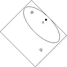
We prove the necessity. For any $x\in\Omega$ there is a cube $Q$ that contains $\Omega$ which is tangent to $\partial\Omega$ at a closest point to $x$ as in the picture:

This cube has fixed dimensions independent of the point $x\in\Omega$ . We can construct a polynomial $Q_{k}^{x}$ of degree at most $kn$ taking the product of one dimensional polynomials $L_{k}^{\frac{1}{2}}$ . We test against these polynomials that peak at $B(x,1/k)$

\int_{B(x,1/k)}|Q_{k}^{x}|^{2}d\mu_{k}\leq\int_{\Omega}|Q_{k}^{x}|^{2}d\mu_{k}\leq C\|Q_{k}^{x}\|_{L^{2}(Q)},

by property $(6)$ in Theorem 3 and the estimate (2.2) the necessary condition follows.

For the sufficiency we use the reproducing property of $L_{k}^{\frac{1}{2}}(z,y)$ . That is for any point $x\in\Omega$ there is a Euclidean ball $\mathbb{B}_{x}$ contained in $\Omega$ such that $x\in\mathbb{B}_{x}$ and it is tangent to $\partial\Omega$ in the closest point to $x$ as in the picture. Moreover since $\Omega$ is a smoothly bounded convex domain we can assume that the radius $\mathbb{B}$ has a lower bound independent of $x$ . In this ball we can reconstruct any polynomial $p\in\mathcal{P}_{k}$ using $L_{k}^{\frac{1}{2}}$ . That is

\int_{\Omega}|p(x)|^{2}\,d\mu_{k}(x)\leq\int_{\Omega}\left|\int_{B_{x}}L_{2k}^{\frac{1}{2}}(x,y)p^{2}(y)\,dV(y)\right|\,d\mu_{k}(x).

We use the estimate (2.4) and we get

\int_{\Omega}|p(x)|^{2}\,d\mu_{k}(x)\lesssim\int_{\Omega}\int_{B_{x}}\frac{\sqrt{\beta_{k}(x)\beta_{k}(y)}}{(1+k\rho(x,y))^{\gamma}}|p(y)|^{2}dV(y)\,d\mu_{k}(x).

We break the integral in two regions, when $\rho(x,y)<1$ and otherwise. When $k$ is big enough we obtain:

\begin{split}\int_{\Omega}|p(x)|^{2}\,d\mu_{k}(x)\leq&\int_{\Omega}\int_{B_{x}\cap\rho(x,y)>1}|p(y)|^{2}dV(y)d\mu_{k}(x)+\\ &C\int_{\Omega}\int_{B_{x}\cap\rho(x,y)<1}\frac{\sqrt{\beta_{k}(x)\beta_{k}(y)}}{(1+k\rho(x,y))^{\gamma}}|p(y)|^{2}dV(y)\,d\mu_{k}(x)\end{split}

The first integral in the right hand side is bounded by $\int_{\Omega}|p(y)|^{2}\,dV(y)$ since $\mu_{k}(\Omega)$ is bounded by hypothesis (it is possible to cover $\Omega$ by balls $\{B(x_{n},1/k)\}$ with controlled overlap).

In the second integral, observe that if $w\in B(x,1/k)$ then $\rho(w,x)\leq 1/k$ and therefore

\frac{\sqrt{\beta_{k}(x)\beta_{k}(y)}}{(1+k\rho(x,y))^{\gamma}}\lesssim\frac{1}{V(B(x,1/k))}\int_{B(x,1/k)}\frac{\sqrt{\beta_{k}(w)\beta_{k}(y)}}{(1+k\rho(w,y))^{\gamma}}dV(w).

We plug this inequality in the second integral and we can bound it by

C\int_{\Omega}|p(y)|^{2}\int_{\rho(w,y)<2}\frac{\sqrt{\beta_{k}(w)\beta_{k}(y)}}{(1+k\rho(w,y))^{\gamma}}\frac{\mu_{k}(B(w,1/k))}{V(B(w,1/k))}dV(w)dV(y).

We use the hypothesis (3.2) and Lemma 4 with $\alpha=1/2$ to bound it finally by $C\int_{\Omega}|p(y)|^{2}dV(y)$ .

∎

The weighted case in the unit ball is simpler.

Theorem 7.

Let $d\mu_{a}(x)=(1-|x|^{2})^{a-\frac{1}{2}}dV(x)$ for $a\geq 0$ the weight in the unit ball $\mathbb{B}\subset\mathbb{R}^{n}.$ A sequence of measures $\{\mu_{k}\}$ are Carleson for $(\mathcal{P}_{k},\mu_{a})$ if there is a constant $C$ such that for all points $x\in\mathbb{B}$

(3.3)

\mu_{k}(B(x,1/k))\leq C\;\mu_{a}(B(x,1/k)).

Proof.

Supose $\{\mu_{k}\}$ are Carleson. Then for any $x\in\mathbb{B}$

(3.4)

\int_{B(x,1/k)}|L_{k}^{a}(x,w)|^{2}\,d\mu_{k}(w)\leq C\|L_{k}^{a}(x,\cdot)\|^{2}_{\mu}.

By property (6) in Theorem 3 and the estimate

K_{k}(\mu,x,x)\leq\|L_{k}^{a}(x,\cdot)\|^{2}_{\mu}\leq K_{2k}(\mu,x,x),

the result follows. The necessity follows exactly like in the unweighted case with the obvious changes. ∎

3.3. Density condition

In [2, Theorem 4] a necessary density condition for sampling sequences for polynomials in convex domains was obtained. It states the following:

Theorem 8.

Let $\Omega$ be a smooth convex domain in $\mathbb{R}^{n}$ , and let $\Lambda$ be a sampling sequence. Then for any $\mathbb{B}(x,r)\subset\Omega$ the following holds:

\limsup_{k\to\infty}\frac{\#\Lambda_{k}\cap\mathbb{B}(x,r)}{\dim\mathcal{P}_{k}}\geq\mu_{eq}(\mathbb{B}(x,r)).

Here $\mu_{eq}$ is the equilibrium measure associated to $\Omega$ .

Let us see how, with a similar technique, a corresponding density condition can be obtained as well in the case of interpolating sequences.

Theorem 9.

Let $\Omega$ be a smooth convex domain in $\mathbb{R}^{n}$ , and let $\Lambda$ be an interpolating sequence. Then for any $\mathbb{B}(x,r)\subset\Omega$ the following holds:

\limsup_{k\to\infty}\frac{\#\Lambda_{k}\cap\mathbb{B}(x,r)}{\dim\mathcal{P}_{k}}\leq\mu_{eq}(\mathbb{B}(x,r)).

Here $\mu_{eq}$ is the equilibrium measure associated to $\Omega$ .

Remark.

In the statements of Theorems 8 and 9 we could have replaced $\mathbb{B}(x,r)$ by any open set, in particular they could have been formulated with balls $B(x,r)$ in the anisotropic metric.

Proof.

Let $F_{k}\subset\mathcal{P}_{k}$ be the subspace spanned by

\kappa_{\lambda}(x)=K_{k}(\lambda,x)/\sqrt{\beta_{k}(\lambda)}\qquad\forall\lambda\in\Lambda_{k}.

Denote by $g_{\lambda}$ the dual (biorthogonal) basis to $\kappa_{\lambda}$ in $F_{k}$ . We have clearly that

•

We can span any function in $F_{k}$ in terms of $\kappa_{\lambda}$ , thus:

$\sum_{\lambda\in\Lambda_{k}}\kappa_{\lambda}(x)g_{\lambda}(x)=\mathcal{K}_{k}(x,x),$

where $\mathcal{K}_{k}(x,y)$ is the reproducing kernel of the subspace $F_{k}$ .
•

The norm of $g_{\lambda}$ is uniformly bounded since $\kappa_{\lambda}$ was a uniform Riesz sequence.
•

$g_{\lambda}(\lambda)=\sqrt{\beta_{k}(\lambda)}$ . This is due to the biorthogonality and the reproducing property.

We are going to prove that the measure $\sigma_{k}=\frac{1}{\dim\mathcal{P}_{k}}\sum_{\lambda\in\Lambda_{k}}\delta_{\lambda}$ , and the measure $\nu_{k}=\frac{1}{\dim\mathcal{P}_{k}}\mathcal{K}_{k}(x,x)d\mu(x)$ are very close to each other. This are two positive measures that are not probability measures but they have the same mass (equal to $\frac{\#\Lambda_{k}}{\dim\mathcal{P}_{k}}\leq 1$ ). Therefore, there is a way to quantify the closeness through the Vaserstein $1$ -distance. For an introduction to Vaserstein distance see for instance [16]. We want to prove that $W(\sigma_{k},\nu_{k})\to 0$ because the Vaserstein distance metrizes the weak-* topology.

In this case, it is known that $\mathcal{K}_{k}(x,x)\leq K_{k}(x,x)$ and $\frac{1}{\dim\mathcal{P}_{k}}\beta_{k}(x)\,\to\mu_{eq}$ in the weak-* topology, where $\mu_{eq}$ is the normalized equilibrium measure associated to $\Omega$ (see for instance [1]). Therefore, $\limsup_{k}\sigma_{k}\leq\mu_{eq}$ .

In order to prove that $W(\sigma_{k},\nu_{k})\to 0$ we use a non positive transport plan as in [11]:

\rho_{k}(x,y)=\frac{1}{\dim\mathcal{P}_{k}}\sum_{\lambda\in\Lambda_{k}}\delta_{\lambda}(y)\times g_{\lambda}(x)\kappa_{\lambda}(x)\,d\mu(x)

It has the right marginals, $\sigma_{k}$ and $\nu_{k}$ and we can estimate the integral

W(\sigma_{k},\nu_{k})\leq\iint_{\Omega\times\Omega}|x-y|d|\rho_{k}|=O(1/\sqrt{k}).

The only point that merits a clarification is that we need an inequality:

\begin{split}\frac{1}{\dim\mathcal{P}_{k}}\sum_{\lambda\in\Lambda_{k}}\int_{\Omega}|\lambda-x|^{2}\frac{|K_{k}(\lambda,x)|^{2}}{K_{k}(x,x)}\,d\mu(x)\leq\\ \frac{1}{\dim\mathcal{P}_{k}}\iint_{\Omega\times\Omega}|y-x|^{2}|K_{k}(y,x)|^{2}\,d\mu(x)d\mu(y).\end{split}

This is problematic. We know that $\Lambda_{k}$ is an interpolating sequence for the polynomials of degree $k$ . Thus the normalized reproducing kernels at $\lambda\in\Lambda_{k}$ form a Bessel sequence for $\mathcal{P}_{k}$ but the inequality that we need is applied to $K_{k}(x,y)(y_{i}-x_{i})$ for all $i=1,\ldots,n$ . That is to a polynomial of degree $k+1$ . We are going to show that if $\Lambda_{k}$ is an interpolating sequence for the polynomials of degree $k$ it is also a Carleson sequence for the polynomials of degree $k+1$ .

Observe that since it is interpolating then it is uniformly separated, i.e. $B(\lambda,\varepsilon/k)$ are disjoint. That means that in particular

\mu_{k}(B(z,1/(k+1))\lesssim V(B(z,1/(k+1)).

Thus $\mu_{k}$ is a Carleson measure for $\mathcal{P}_{k+1}$ .

Finally in [2, Theorem 17] it was proved that

\frac{1}{\dim\mathcal{P}_{k}}\iint_{\Omega\times\Omega}|y-x|^{2}|K_{k}(y,x)|^{2}\,d\mu(x)d\mu(y)=O(1/k).

∎

From the behaviour on the diagonal of the kernel (2.2) its easy to check that the kernel is both Bernstein-Markov (sub-exponential) and has moderate growth, see definitions in [2]. From the characterization for sampling sequences proved in [2, Theorem 1] and with the obvious changes in the proof of the previous theorem we deduce the following:

Theorem 10.

Consider the space of polynomials $\mathcal{P}_{k}$ restricted to the ball $\mathbb{B}\subset\mathbb{R}^{n}$ with the measure $d\mu_{a}(x)=(1-|x|^{2})^{a-\frac{1}{2}}dV.$ Let $\Lambda=\{\Lambda_{k}\}$ be a sequence sets of points in $\mathbb{B}.$

•

If $\Lambda$ is a sampling sequence

$\liminf_{k\to\infty}\frac{\#(\Lambda_{k}\cap\mathbb{B}(x,r))}{\dim\mathcal{P}_{k}}\geq\mu_{eq}(\mathbb{B}(x,r)).$
•

If $\Lambda$ is interpolating

$\limsup_{k\to\infty}\frac{\#(\Lambda_{k}\cap\mathbb{B}(x,r))}{\dim\mathcal{P}_{k}}\leq\mu_{eq}(\mathbb{B}(x,r)).$

Remark.

One can construct interpolation or sampling sequences with density arbitrary close to the critical density with sequences of points $\{\Lambda_{k}\}$ such that the corresponding Lagrange interpolating polynomials are uniformly bounded. In particular de above inequalities are sharp, for a similar construction on the sphere see [12].

3.4. Orthonormal basis of reproducing kernels

Sampling and interpolation are somehow dual concepts. Sequences which are both sampling and interpolating (i.e. complete interpolating sequences) are optimal in some sense because they are at the same time minimal sampling sequences and maximal interpolating sequences. They will satisfy the equality in Theorem 10. In general domains, to prove or disprove the existence of such sequences is a difficult problem [13].

If $\Lambda=\{\Lambda_{k}\}$ is a complete interpolating sequence the corresponding reproducing kernels $\{\kappa_{k,\lambda}\}$ is a Riesz basis in the space of polynomials (uniformly in the degree). An obvious example of complete interpolating sequences would be sequences providing an orthonormal basis of reproducing kernels. In dimension 1, with the weight $(1-x^{2})^{a-1/2},$ a basis of Gegenbauer polynomials $\{G^{(a)}_{j}\}_{j=0,\dots,k}$ is orthogonal and the reproducing kernel in $\mathcal{P}_{k}$ evaluated at the zeros of the polynomial $G^{(a)}_{k+1}$ gives an orthogonal sequence. In our last result we prove that for greater dimensions there are no orthogonal basis of $\mathcal{P}_{k}$ of reproducing kernels with the measure $d\mu_{a}(x)=(1-|x|^{2})^{a-1/2}dV(x).$

Our first goal is to show that sampling sequences are dense enough, Theorem 12. Recall that in the bulk (i.e. at a fixed positive distance from the boundary) the Euclidean metric and the metric $\rho$ are equivalent. In our first result we prove that the right hand side of (1.3) and the separation imply that there are points of the sequence in any ball (of the bulk) of big enough radius.

Proposition 11.

Let $d\mu_{a}(x)=(1-|x|^{2})^{a-\frac{1}{2}}dV(x)$ for $a\geq 0$ the weight in the unit ball $\mathbb{B}\subset\mathbb{R}^{n}.$ Let $\Lambda_{k}\subset\mathbb{B}$ be a finite subset and $C,\epsilon>0$ be constants such that

(3.5)

\int_{\mathbb{B}}|P(x)|^{2}d\mu_{a}(x)\leq C\sum_{\lambda\in\Lambda_{k}}\frac{|P(\lambda)|^{2}}{K_{k}(\mu_{a};\lambda,\lambda)},

for all $P\in\mathcal{P}_{k}$ and

\inf_{\begin{subarray}{c}\lambda,\lambda^{\prime}\in\Lambda_{k}\\ \lambda\neq\lambda^{\prime}\end{subarray}}\rho(\lambda,\lambda^{\prime})\geq\frac{\epsilon}{k}.

Let $|x_{0}|=C_{0}<\frac{1}{4},$ $\epsilon<M$ and $k\geq 1$ be such that $\Lambda_{k}\cap\mathbb{B}(x_{0},M/k)=\emptyset.$ Then $M<A$ for a certain constant $A$ depending only on $C,\epsilon,n$ and $a.$

Proof.

By the construction of function $L_{\ell}^{a}(x,y),$ it is clear that for any $\ell\geq 0$

K_{\ell}(\mu_{a};x,x)\leq\int_{\mathbb{B}}L_{\ell}^{a}(x,y)^{2}d\mu_{a}(y)\leq K_{2\ell}(\mu_{a};x,x).

Let $P(x)=L^{a}_{[k/2]}(x,x_{0})\in\mathcal{P}_{k}.$ From the property above, the hypothesis and Proposition 2 we get

(3.6)

k^{n}\sim K_{[k/2]}(\mu_{a};x_{0},x_{0})\leq\int_{\mathbb{B}}P(y)^{2}d\mu_{a}(y)\lesssim\sum_{|\lambda-x_{0}|>M/k}\frac{|P(\lambda)|^{2}}{K_{k}(\mu_{a};\lambda,\lambda)}.

From [6, Lemma 11.3.6.], given $x\in\mathbb{B}$ and $0<r<\pi$

(3.7)

\mu_{a}(B(x,r))\sim r^{n}(\sqrt{1-|x|^{2}}+r)^{2a},

and therefore

(3.8)

\mu_{a}(B(x,r))\sim\begin{cases}r^{n+2a}&\mbox{if}\;\;1-|x|^{2}<r^{2},\\ r^{n}(1-|x|^{2})^{a}&\mbox{otherwise},\end{cases}

and

(3.9)

\mu_{a}(B(x,r))\gtrsim\begin{cases}r^{n+2a}&\mbox{if}\;\;|x|>\frac{1}{2},\\ r^{n}&\mbox{otherwise}.\end{cases}

From (4) in Theorem 3, the separation of the sequence, and the estimate (3.9) we get

(3.10)

\begin{split}0&<c\leq\sum_{|\lambda-x_{0}|>M/k}\frac{1}{(1+[k/2]\rho(x_{0},\lambda))^{2\gamma}}\\ &=\sum_{|\lambda-x_{0}|>M/k}\frac{1}{\mu_{a}(B(\lambda,\epsilon/2k))}\int_{B(\lambda,\epsilon/2k)}\frac{d\mu_{a}(x)}{(1+[k/2]\rho(x_{0},\lambda))^{2\gamma}}\\ &\lesssim\left[\sum_{\frac{M}{k}<|\lambda-x_{0}|<\frac{1}{2}}+\sum_{\frac{1}{2}<|\lambda-x_{0}|}\right]\frac{1}{\mu_{a}(B(\lambda,\epsilon/2k))}\int_{B(\lambda,\epsilon/2k)}\frac{d\mu_{a}(x)}{(1+2k\rho(x_{0},x))^{2\gamma}}\\ &\lesssim\left(\frac{k}{\epsilon}\right)^{n}\int_{\frac{M}{k}}^{\frac{3}{4}}\frac{r^{n-1}}{(kr)^{2\gamma}}dr+\frac{k^{2a+n-2\gamma}}{\epsilon^{2a+n}}\mu_{a}(B(0,1/2)^{c}).\end{split}

Now, for $\gamma=n+a$ we get

0<c\leq\frac{1}{k^{n+2a}}\left[-\frac{1}{r^{n+2a}}\right]_{r=\frac{M}{k}}^{\frac{3}{4}}+\frac{1}{k^{n}},

and then a uniform (i.e. independent of $k$ ) upper bound for $M<A=A(C,\epsilon,n,a).$ ∎

Proposition 12.

Let $\Lambda=\{\Lambda_{k}\}$ be a separated sampling sequence for $\mathbb{B}\subset\mathbb{R}^{n}.$ Then there exist $M_{0},k_{0}>0$ such that for any $M>M_{0}$ and all $k\geq k_{0}$

\#\left(\Lambda_{k}\cap\mathbb{B}(0,M/k)\right)\sim M^{n}.

Proof.

Let $\epsilon>0$ be the constant from the separation, i.e.

\inf_{\begin{subarray}{c}\lambda,\lambda^{\prime}\in\Lambda_{k}\\ \lambda\neq\lambda^{\prime}\end{subarray}}\rho(\lambda,\lambda^{\prime})\geq\frac{\epsilon}{k}.

Assume that $M/k\leq\frac{1}{2}.$ For $\lambda\in\Lambda_{k}\cap\mathbb{B}(0,M/k)$ we have $V(\mathbb{B}(\lambda,\frac{\epsilon}{k}))\sim(\frac{\epsilon}{k})^{n}$ and therefore

(3.11)

\#\left(\Lambda_{k}\cap\mathbb{B}(0,M/k)\right)\left(\frac{\epsilon}{k}\right)^{n}\lesssim\left(\frac{M}{k}\right)^{n}.

For the other inequality, take the constant $A$ (assume $A>\epsilon$ ) given in Proposition 11 depending on the sampling and the separation constants of $\Lambda$ and $n.$ For $M>A$ and $k>0$ such that $\mathbb{B}(0,\frac{M}{k})\subset\mathbb{B}(0,\frac{1}{4})$ one can find $N$ disjoint balls $\mathbb{B}(x_{j},\frac{A}{k})$ for $j=1,\dots N$ included in $\mathbb{B}(0,M/k)$ and such that

NV(\mathbb{B}(0,\frac{A}{k}))>\frac{1}{2}V(\mathbb{B}(0,\frac{M}{k})).

Observe that each ball $\mathbb{B}(x_{j},\frac{A}{k})$ contains by Proposition 11 at least one point from $\Lambda_{k}$ and therefore

\#\left(\Lambda_{k}\cap\mathbb{B}(0,M/k)\right)\geq N\gtrsim\left(\frac{M}{A}\right)^{n}.

∎

We will use the following result from [8].

Theorem 13.

Let $\mathbb{B}\subset\mathbb{R}^{n},$ $n>1,$ be the unit ball. There do not exist infinite subsets $\Lambda\subset\mathbb{R}^{n}$ such that the exponentials $e^{i\langle x,\lambda\rangle},$ $\lambda\in\Lambda,$ are pairwise orthogonal in $L^{2}(\mathbb{B}).$ Or, equivalently, there do not exist infinite subsets $\Lambda\subset\mathbb{R}^{n}$ such that $|\lambda-\lambda^{\prime}|$ is a zero of $J_{n/2},$ the Bessel function of order $n/2,$ for all distinct $\lambda,\lambda^{\prime}\in\Lambda.$

Following ideas from [7] we can prove now our main result about orthogonal basis. A similar argument can be used on the sphere to study tight spherical designs.

Theorem 14.

Let $\mathbb{B}\subset\mathbb{R}^{n}$ be the unit ball and $n>1.$ There is no sequence of finite sets $\Lambda=\{\Lambda_{k}\}\subset\mathbb{B}$ such that the reproducing kernels $\{K_{k}(\mu:x,\lambda)\}_{\lambda\in\Lambda_{k}}$ form an orthogonal basis of $\mathcal{P}_{k}$ with respect to the measure $d\mu_{a}=(1-|x|^{2})^{a-\frac{1}{2}}dV$ .

Theorem 14.

The following result can be easily deduced from [10, Theorem 1.7]:

Given $\{u_{k}\}_{k},\{v_{k}\}_{k}$ convergent sequences in $\mathbb{R}^{n}$ and $u_{k}\to u,v_{k}\to v,$ when $k\to\infty.$ Then

\lim_{k\to\infty}\frac{K_{k}(\mu;\frac{u_{k}}{k},\frac{v_{k}}{k})}{K_{k}(\mu;0,0)}=\frac{J^{*}_{n/2}(|u-v|)}{J^{*}_{n/2}(0)}.

Let $\Lambda_{k}$ be such that $\{\kappa_{\lambda}\}_{\lambda\in\Lambda_{k}}$ is an orthonormal basis of $\mathcal{P}_{k}$ with respect to the measure $d\mu_{a}=(1-|x|^{2})^{a-\frac{1}{2}}dV$ . Then

K_{k}(\mu;\lambda_{(k)},\lambda_{(k)}^{\prime})=0,

for $\lambda_{(k)}\neq\lambda_{(k)}^{\prime}\in\Lambda_{k}.$

We know that $\Lambda_{k}$ is uniformly separated for some $\epsilon>0$

\rho(\lambda_{(k)},\lambda_{(k)}^{\prime})\geq\frac{\epsilon}{k}.

Then the sets $X_{k}=k(\Lambda_{k}\cap\mathbb{B}(0,1/2))\subset\mathbb{R}^{n}$ are uniformly separated

|\lambda-\lambda^{\prime}|\gtrsim\epsilon,\;\;\lambda\neq\lambda^{\prime}\in X,

and $X_{k}$ converges weakly to some uniformly separated set $X\subset\mathbb{R}^{n}.$ The limit is not empty because by Proposition 12 for any $M>0,$

\#\left(\Lambda_{k}\cap\mathbb{B}(0,M/k)\right)\sim M^{d}.

Observe that this last result would be a direct consequence of the necessary density condition for complete interpolating sets if we could take balls of radius $r/n$ for a fixed $r>0$ in the condition. Finally, we obtain an infinite set $X$ such that for $\lambda\neq\lambda^{\prime}\in X$

J^{*}_{n/2}(|\lambda-\lambda^{\prime}|)=0,

in contradiction with Theorem 13. ∎

Remark.

Note that the fact that the interpolating sequence $\{\Lambda_{k}\}$ is complete was used only to guarantee that $\#\left(\Lambda_{k}\cap\mathbb{B}(0,M/k)\right)\sim M^{d}$ . So, the above result could be extended to sequences $\{\Lambda_{k}\}$ such that $\{\kappa_{k,\lambda}\}_{\lambda\in\Lambda_{k}}$ is orthonormal (but not necessarily a basis for $\mathcal{P}_{k}$ ) if $\Lambda_{k}\cap\mathbb{B}(0,M/k)$ contains enough points.

References

[1] R. Berman, S. Boucksom, D.W. Nyström Fekete points and convergence towards equilibrium measures on complex manifolds, Acta Math (2011) 207, 1-27.
[2] R. Berman, J. Ortega-Cerdà. Sampling of real multivariate polynomials and pluripotential theory. Amer. Journal of Math. 140 n. 3 (2018), pp. 789-820.
[3] E. Bedford, A. Taylor, The complex equilibrium measure of a symmetric convex set in $\mathbb{R}^{n}$ . Trans. Amer. Math. Soc. 294 (1986), pp. 705-717.
[4] L. Bos, Asymptotics for the Christoffel function for Jacobi like weights on a ball in $\mathbb{R}^{m},$ New Zealand J. Math. 23 (1994), no. 2, 99-109.
[5] D. Burns, N. Levenberg, S. Ma’u, Sz. Révész, Monge-Ampère measures for convex bodies and Bernstein-Markov type inequalities. Trans. Amer. Math. Soc. 362 (2010), no. 12, pp. 6325-6340.
[6] F. Dai, Y. Xu, Approximation theory and harmonic analysis on spheres and balls, Springer Monographs in Mathematics, Springer, New York, 2013.
[7] B. Fuglede, Commuting self-adjoint partial differential operators and a group theoretic problem, J. Funct. Math., 16, 1974, 101-121.
[8] B. Fuglede, Orthogonal exponentials on the ball, Expo.Math. 19 (2001), 267-272.
[9] M. Klimek, Pluripotential Theory, Oxford University Press, New York, 1991.
[10] A. Kroó, D. S. Lubinsky, Christoffel functions and universality in the bulk for multivariate orthogonal polynomials. Canad. J. Math. 65 (2013), no. 3, 600–620.
[11] N. Lev, J. Ortega-Cerdà, Equidistribution estimates for Fekete points on complex manifolds, J. Eur. Math. Soc. (JEMS) 18 (2016), no. 2, 425-464
[12] J. Marzo, J. Ortega-Cerdà, Equidistribution of the Fekete points on the sphere, Constr. Approx., 32, 3 (2010), 513-521
[13] A. Olevskii, A. Ulanovskii, Functions with disconnected spectrum. Sampling, interpolation, translates, University Lecture Series, 65. American Mathematical Society, Providence, RI, 2016.
[14] P. Petrushev, Y. Xu, Localized polynomial frames on the ball. Constr. Approx. 27 (2008), pp. 121-148.
[15] H. S. Shapiro, A. L. Shields, On some interpolation problems for analytic functions. Amer. J. Math. 83 (1961), pp. 513-532.
[16] C. Villani. Optimal transport, v. 338 of Grundlehren der Mathematischen Wissenschaften, Springer-Verlag, Berlin, 2009.
[17] Y. Xu, Summability of Fourier orthogonal series for Jacobi weight on a ball in $\mathbb{R}^{d}$ , Trans. Amer. Math. Soc., 351 (1999), pp. 2439-2458.