On the Non-Monotonicity of a Non-Differentially Mismeasured Binary Confounder
Abstract.
Suppose that we are interested in the average causal effect of a binary treatment on an outcome when this relationship is confounded by a binary confounder. Suppose that the confounder is unobserved but a non-differential binary proxy of it is observed. We identify conditions under which adjusting for the proxy comes closer to the incomputable true average causal effect than not adjusting at all. Unlike other works, we do not assume that the average causal effect of the confounder on the outcome is in the same direction among treated and untreated.
1. Introduction
Suppose that we are interested in the average causal effect of a binary treatment on an outcome when this relationship is confounded by a binary confounder . Suppose also that is non-differentially mismeasured, meaning that (i) is not observed and, instead, a binary proxy of is observed, and (ii) is conditionally independent of and given . The causal graph to the left in Figure 1 represents the relationships between the random variables.
Greenland 1980 argues that adjusting for produces a partially adjusted measure of the average causal effect of on that is between the crude (i.e., unadjusted) and the true (i.e., adjusted for ) measures and, thus, it comes closer to the incomputable true measure than the crude one. Ogburn and VanderWeele 2012 show that, although this result does not always hold, it does hold under some monotonicity condition in . Specifically, must be non-decreasing or non-increasing in . Unfortunately, the condition cannot be verified empirically because is unobserved. Ogburn and VanderWeele 2013 extend these results to the case where takes more than two values. Peña 2020 shows that if is non-decreasing or non-increasing in (which can be verified empirically), then so is with respect to and, thus, the partially adjusted average causal effect lies between the crude and the true ones. Finally, if there are at least two independent proxies of , then Miao et al. 2018 show that the average causal effect of on can be identified under certain rank condition.
In this paper, we focus on the case where neither nor are monotone in or . And we report conditions under which the partially adjusted average causal effect is still between the crude and the true ones and, thus, it is still closer to the incomputable true average causal effect. Specifically, the rest of the paper is organized as follows. Sections 2 and 3 report the novel conditions. Section 4 deals with continuous random variables. Section 5 closes with some discussion.
2. Bounding the Observed Risk Difference
Consider the causal graph to the left in Figure 1, where is a discrete or continuous random variable, and , and are binary random variables. The graph entails the following factorization:
| (1) |
Let take values and , and similarly for and . Let , and be observed and let be unobserved. Let and denote the counterfactual outcomes under treatments and , respectively. The average causal effect of on or true risk difference () is defined as . It can be rewritten as follows (Pearl 2009, Theorem 3.3.2):
Since is unobserved, cannot be computed. However, it can be approximated by the unadjusted average causal effect or crude risk difference ():
and by the partially adjusted average causal effect or observed risk difference ():
Now the question is, which of the two approximations comes closer to the true quantity ? This paper aims to answer this question.
We say that is non-decreasing in if
Likewise, is non-increasing in if
Moreover, is monotone in if it is non-decreasing or non-increasing in , i.e. the average causal effect of on is in the same direction among the treated () and the untreated (). Ogburn and VanderWeele 2012 show that if is monotone in , then lies between and and, thus, it comes closer to than . Unfortunately, the antecedent of this rule cannot be verified empirically, because is unobserved. Therefore, one must rely on substantive knowledge to apply the rule. Peña 2020 shows that if is monotone in , then lies between and . Note that the antecedent of this rule can be verified empirically. Actually, is monotone in if and only if is monotone in (Ogburn and VanderWeele 2012; Peña 2020).
Peña 2020 characterizes a case where is not monotone in and, thus, is not monotone in , and yet lies between and . We re-state this result in the next theorem. Note that one must rely on substantive knowledge to verify the conditions in the theorem.
Theorem 1 (Peña, 2020, Theorems 3 and 4).
Consider the causal graph to the left in Figure 1. Let and . If , then . If , then .
The following theorems are the main contribution of this work. They show that the conditions in the previous theorem can be relaxed. Their proofs can be found in the supplementary material.
Theorem 2.
Consider the causal graph to the left in Figure 1. Let , and . Then, lies between and .
Theorem 3.
Consider the causal graph to the left in Figure 1. Let , and . Then, lies between and .
The following example gives some intuition about the conditions in Theorem 2. Let , and represent three diseases, and a gene variant that affects the three of them. Moreover, suppose that suffering affects the risk of suffering . Suppose also that half of the population carries the gene variant , i.e. . Suppose also that carrying predisposes to suffer and as much as not carrying it protects against the diseases, i.e. and . Then, the theorem applies.
Corollary 4.
Consider the causal graph to the left in Figure 1. Let , and . If , then . If , then .
Corollary 5.
Consider the causal graph to the left in Figure 1. Let , and . If , then . If , then .
To get some intuition about the conditions for the first result in Corollary 4, let us extend the previous example with the following additional assumption: Carrying the gene variant increases the average severity of for the individuals suffering more than it decreases the severity for the rest. Then, the corollary applies.
Note that one must rely on substantive knowledge to verify the conditions in the previous theorems and corollaries. The next two corollaries show that this can partially be alleviated by replacing the conditions on with similar conditions on : The former are not empirically testable because is unobserved, but the latter are.
Corollary 6.
Under the conditions in Corollary 4, if and only if . Likewise when replacing with .
Corollary 7.
Under the conditions in Corollary 5, if and only if . Likewise when swapping and .
 |
 |
 |
 |
2.1. Experiments
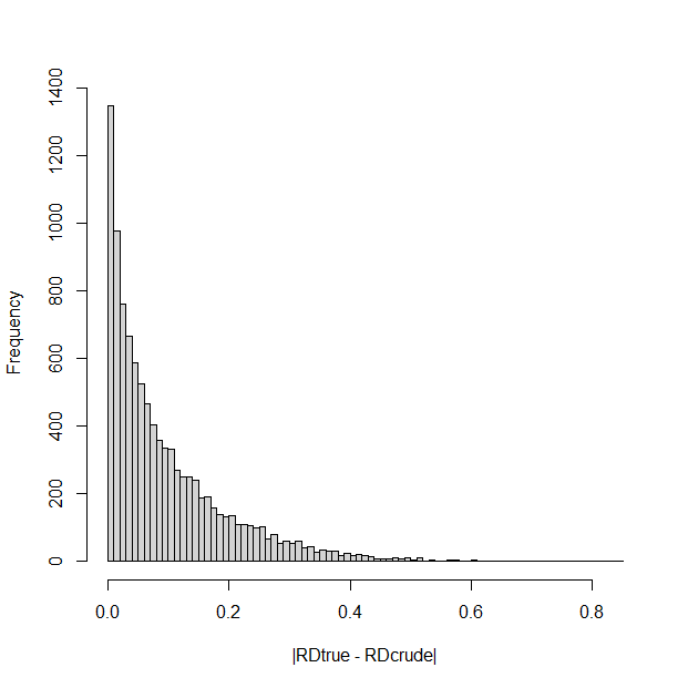
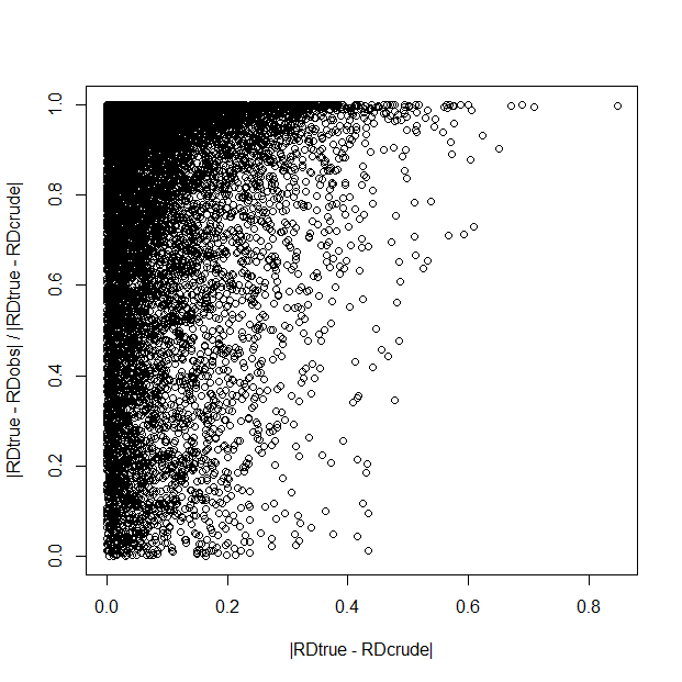
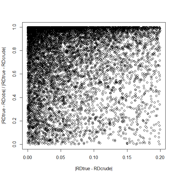
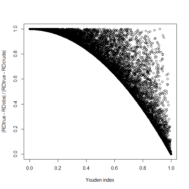
In this section, we report some experiments that shed additional light on the relationships between the various risk differences under the conditions in Theorem 2. For the experiments, we let be binary. Then, we randomly parameterize 10000 times the causal graph to the left in Figure 1 by parameterizing the terms in the right-hand side of Equation 1 with parameter values drawn from a uniform distribution, while enforcing the assumptions in the theorem. For each parameterization, we compute , and . Figure 2 summarizes the results.11 1 Code available at https://www.dropbox.com/s/t75z8yro1e9higq/nonmonotonicity3.R?dl=0. The top left plot shows that most intervals are relatively small and, thus, that is close to in most cases. However, the top right plot shows that tends to be closer to than to . The bottom left plot is a zoom of the previous plot at the smallest intervals. Finally, the bottom right plot shows that the stronger the dependence between and as measured by the Youden index (i.e., ), the closer is to . In summary, is a reasonable approximation to , but it is biased towards . This may be a problem when the interval between and is large. However, the length of the interval is unknown in practice, and we doubt substantive knowledge may provide hints on it. The bias decreases with increasing dependence between and . Although the strength of this dependence is unknown in practice, substantive knowledge may give hints on it.
3. Bounding the True Risk Difference
Theorems and Corollaries 1-5 do not hold if the assumption that is replaced by the weaker assumption that . Likewise for the assumption that . However, Peña 2020 proves that the assumption can be relaxed and still and bound . We re-state this result in the next theorem.
Theorem 8 (Peña, 2020, Theorems 5 and 6).
Consider the causal graph to the left in Figure 1. Let , and . If , then and . If , then and .
Note that the previous theorem does not determine the order between and . Thus, it cannot be used to decide which of the two comes closer to . However, the theorem may be useful to conclude whether is positive or negative. For instance, the last result in the theorem allows us to conclude that whenever .
The following theorems show that the assumption that in the previous theorem can also be relaxed.
Theorem 9.
Consider the causal graph to the left in Figure 1. Let , and . If , then and . If , then and .
Theorem 10.
Consider the causal graph to the left in Figure 1. Let , and . If , then and . If , then and .
Returning to our example of three diseases , and and a gene variant , the assumptions for the first result in Theorem 9 mean that (i) half of the population carry the gene variant , i.e. , (ii) not carrying protects against and more than carrying it predisposes to suffer the diseases, i.e. and , and (iii) carrying increases the average severity of for the individuals suffering more than it decreases the severity for the rest.
The last two theorems can be strengthened for as follows. Analogous results do not hold for , though.
Theorem 11.
Consider the causal graph to the left in Figure 1. Let and . If , then . If , then .
Theorem 12.
Consider the causal graph to the left in Figure 1. Let and . If , then . If , then .
4. Path Diagrams
Finally, we suppose that the variables , , and are all continuous and follow the linear structural equation model represented by the path diagram to the right in Figure 1. The true, crude and partially adjusted average causal effects of on are given by the partial regression coefficients , and , respectively. Note that the first cannot be computed because is unobserved. The following theorem proves that the partially adjusted average causal effect lies between the true and the crude ones and, thus, it comes closer to the true average causal effect than the crude.
Theorem 13.
Consider the path diagram to the right in Figure 1. Assume that the variables are standardized. If then , else .
Note that unlike in the discrete case, no assumptions about the causal relationships of the variables are required to conclude that the partially adjusted average causal effect lies between the true and the crude ones. Note also that the signs of and tell us whether the partially adjusted average causal effect is an upper or lower bound of the true one.
5. Discussion
One may think that adjusting for a proxy of a latent confounder is always a good idea. However, it is not. In this work, we have described sufficient conditions under which adjusting for a proxy of a latent confounder comes closer to the incomputable true average causal effect than not adjusting at all. Under some conditions, it is even possible to decide whether the partially adjusted approximation is an upper or a lower bound of the true quantity. We have experimentally shown that the partially adjusted approximation can be substantially better than the unadjusted one when the dependence between confounder and proxy is significant. We have also illustrated with an example that the conditions proposed are not too restrictive and unrealistic. Since one must rely on expert knowledge to verify the conditions, we would like to investigate in the future whether realistic, sufficient and empirically testable conditions exist. We would also like to extend this work to when several latent confounders exist.
Acknowledgments
This work was funded by the Swedish Research Council (ref. 2019-00245).
Supplementary Material: Proofs
Theorem 2.
Consider the causal graph to the left in Figure 1. Let , and . Then, lies between and .
Proof.
We start by establishing a relationship between and . First, note that
where
is known as the log odds, and is known as the logistic sigmoid function (Bishop 2006, Section 4.2). Then,
| (2) |
where the second equality follows from the assumption that , and the fact that and are conditionally independent given due to the causal graph under consideration. Likewise,
| (3) |
and
| (4) |
and
| (5) |
Then, and because and are increasing functions and by the assumption that . Then,
| (6) |
by the assumption that . Moreover,
| (7) |
Next, note that
| (8) |
by the assumptions that and . Likewise,
| (9) |
Then,
| (10) |
because
| (11) |
Moreover,
| (12) |
Finally, Equations Proof. and 10 allow us to write with , whereas Equations 7, 10 and 12 allow us to write . Therefore,
where the third equality follows from the fact that and are conditionally independent given and due to the causal graph under consideration. Then,
| (13) |
with .
We continue by establishing a similar relationship between and . First, note that
| (14) | ||||
by the fact that and are conditionally independent given due to the causal graph under consideration, the assumption that , and the fact that which follows from the assumptions that and and the fact that as shown in Equation 11. Likewise,
| (15) | ||||
Next, let and . Recall that by assumption, and as shown above. Then, Equation Proof. can be rewritten as
Recall that by assumption. If , then . On the other hand, if then . To see it, assume to the contrary that
which contradicts the assumption that . Consequently, and by Equations Proof. and Proof..
Finally, note that
by the assumptions that and . This together with the fact that as shown in Equation 11, and the previous paragraph imply that and . Let and with . Then,
| (16) |
with , where the last equality follows from the fact that by Equation 11.
Now, note that
| (17) |
where the second equality follows from the fact that and are conditionally independent given and due to the causal graph under consideration. Likewise,
| (18) |
where the last equality follows from Equations 8 and 9. Moreover, Equations 8 and 9 also imply that , because by assumption. Then,
| (19) |
This equation together with Equations 13 and Proof. imply the desired result. ∎
Theorem 3.
Consider the causal graph to the left in Figure 1. Let , and . Then, lies between and .
Proof.
Similar to the proof of Theorem 2. Specifically, the assumption that implies that , which implies that and , which implies that , which implies that
| (20) |
with . Likewise, the assumption that implies that and , which implies that and , which implies that
| (21) |
with . The assumption that also implies that , which implies that
| (22) |
This equation together with Equations 20 and 21 imply the desired result. ∎
Corollary 4.
Consider the causal graph to the left in Figure 1. Let , and . If , then . If , then .
Corollary 5.
Consider the causal graph to the left in Figure 1. Let , and . If , then . If , then .
Corollary 6.
Under the conditions in Corollary 4, if and only if . Likewise when replacing with .
Proof.
Corollary 7.
Under the conditions in Corollary 5, if and only if . Likewise when swapping and .
Proof.
Theorem 9.
Consider the causal graph to the left in Figure 1. Let , and . If , then and . If , then and .
Proof.
We start by proving the first result in the theorem, specifically that . Recall from the proof of Theorem 2 that
where the second equality follows from the assumption that . Likewise,
Therefore, and due to the assumption that . Now, consider the function . By inspecting the first and second derivatives, we can conclude that has a single maximum at , and that it is increasing in the interval and decreasing in the interval . This implies that due to the assumption that . Then,
| (23) |
which together with the fact that and are increasing functions imply that .
The results in the previous paragraph allow us to write and with . Therefore,
| (24) |
which implies that because , and by assumption.
We continue by proving that . First, recall Equations 2-5. Then, and because and are increasing functions and by the assumption that . Then,
by the assumption that . We can analogously prove that . Moreover, it also holds that
To prove this inequality and after failing to do it on our own, we resorted to the function FindInstance from Mathematica 12.2.0. Specifically, we used FindInstance to find an instance of the probabilities that satisfied the reverse of the inequality above subject to , and . Since no such instance was found, the inequality above must hold. It is worth mentioning that FindInstance works analytically and not numerically and, thus, its outcome is exact and correct.22 2 Code available at https://www.dropbox.com/s/i8pnmm9zz4pqmgp/inequality.nb?dl=0.
The results in the previous paragraph allow us to write and with . Consequently, , and . Therefore,
| (25) |
where the third equality follows from the fact that and are conditionally independent given and due to the causal graph under consideration. Then, because , and by assumption.
Theorem 10.
Consider the causal graph to the left in Figure 1. Let , and . If , then and . If , then and .
Proof.
Similar to the proof of Theorem 9. Specifically, the assumption that implies that , which together imply that , which implies that
with . This implies the stated relationships between and . The assumption that also implies that , which implies that and , which together with the assumption that imply that
which implies that
with . This implies the stated relationships between and . ∎
Theorem 11.
Consider the causal graph to the left in Figure 1. Let and . If , then . If , then .
Proof.
Recall from the proof of Theorem 2 that
and
and
and
Therefore, and because and are increasing functions and and by the assumption that . Then, we can write and with . Moreover, . To see it, recall from the proof of Theorem 9 that a function of the form has a single maximum at , and it is increasing in the interval and decreasing in the interval . Now, note that (Bishop 2006, Equation 4.88). Then, has a single maximum at (i.e. at ), and it is increasing in the interval (i.e., ) and decreasing in the interval (i.e., ). In other words, increases at an increasing rate in the interval and increases at a decreasing rate in the interval . Therefore, for all . Then,
where the first inequality follows from the fact that with and , and the second inequality follows from Equation 23 and the fact that and are increasing functions. Note that by the assumptions that and .
Finally, note that
| (26) |
which implies the desired results because . ∎
Theorem 12.
Consider the causal graph to the left in Figure 1. Let and . If , then . If , then .
Proof.
Theorem 13.
Consider the path diagram to the right in Figure 1. Assume that the variables are standardized. If then , else .
Proof.
Pearl 2013 shows that , and
| (27) |
Note that the linear structural equation model corresponding to the path diagram under consideration implies that
where is an error term that is independent of and, thus,
where due to the assumption that the variables are standardized. This implies that . Similarly . Then, in Equation 27. The result is now immediate. ∎
References
- Bishop (2006) C. M. Bishop. Pattern Recognition and Machine Learning. Springer, 2006.
- Greenland (1980) S. Greenland. The Effect of Misclassification in the Presence of Covariates. American Journal of Epidemiology, 112(4):564–569, 1980.
- Miao et al. (2018) W. Miao, Z. Geng, and E. J. Tchetgen Tchetgen. Identifying Causal Effects with Proxy Variables of an Unmeasured Confounder. Biometrika, 105(4):987–993, 2018.
- Ogburn and VanderWeele (2012) E. L. Ogburn and T. J. VanderWeele. On the Nondifferential Misclassification of a Binary Confounder. Epidemiology, 23(3):433–439, 2012.
- Ogburn and VanderWeele (2013) E. L. Ogburn and T. J. VanderWeele. Bias Attenuation Results for Nondifferentially Mismeasured Ordinal and Coarsened Confounders. Biometrika, 100(1):241–248, 2013.
- Peña (2020) J. M. Peña. On the Monotonicity of a Nondifferentially Mismeasured Binary Confounder. Journal of Causal Inference, 8:150–163, 2020.
- Pearl (2009) J. Pearl. Causality: Models, Reasoning, and Inference. Cambridge University Press, 2009.
- Pearl (2013) J. Pearl. Linear Models: A Useful “Microscope” for Causal Analysis. Journal of Causal Inference, 1:155–170, 2013.