Equivalence of measures and asymptotically optimal linear prediction for Gaussian random fields with fractional-order covariance operators

David Bolinlabel=e1]david.bolin@kaust.edu.sa Email: [ Kristin Kirchnerlabel=e2 Email: [ mark]k.kirchner@tudelft.nl Address: CEMSE Division, King Abdullah University of Science and Technology, Thuwal, Saudi Arabia Address: Delft Institute of Applied Mathematics, Delft University of Technology, Delft, The Netherlands

Abstract

We consider Gaussian measures $\mu,\widetilde{\mu}$ on a separable Hilbert space, with fractional-order covariance operators $A^{-2\beta}$ resp. $\widetilde{A}^{-2\widetilde{\beta}}$ , and derive necessary and sufficient conditions on $A,\widetilde{A}$ and $\beta,\widetilde{\beta}>0$ for I. equivalence of the measures $\mu$ and $\widetilde{\mu}$ , and II. uniform asymptotic optimality of linear predictions for $\mu$ based on the misspecified measure $\widetilde{\mu}$ . These results hold, e.g., for Gaussian processes on compact metric spaces. As an important special case, we consider the class of generalized Whittle–Matérn Gaussian random fields, where $A$ and $\widetilde{A}$ are elliptic second-order differential operators, formulated on a bounded Euclidean domain $\mathcal{D}\subset\mathbb{R}^{d}$ and augmented with homogeneous Dirichlet boundary conditions. Our outcomes explain why the predictive performances of stationary and non-stationary models in spatial statistics often are comparable, and provide a crucial first step in deriving consistency results for parameter estimation of generalized Whittle–Matérn fields.

Keywords:

Whittle–Matérn fields.,

keywords

^†^†email: e1^†^†email: e2

and

1 Introduction and preliminaries

1.1 Introduction

Equivalence and orthogonality of Gaussian measures are essential concepts for investigating asymptotic properties of Gaussian random fields and stochastic processes. For example, they play a crucial role when proving consistency of maximum likelihood estimators for covariance parameters under infill asymptotics [2, 41], or asymptotic optimality of linear predictions for random fields based on misspecified covariance models [36]. However, for the latter equivalence of the Gaussian measures is not a necessary assumption. This is an immediate consequence of the necessary and sufficient conditions for uniformly asymptotically optimal linear prediction, derived recently in [26] for Gaussian random fields on compact metric spaces. Both the necessary and sufficient conditions for equivalence of Gaussian measures as given by the Feldman–Hájek theorem [12, Theorem 2.25] and those for uniformly asymptotically optimal linear prediction [26, Assumption 3.3] are formulated in terms of the covariance operators rather than the covariance functions. Therefore, they may be difficult to verify. To the bestof our knowledge there are not even sufficient conditions for asymptotic optimality available, which are easily verifiable, except for a few special cases such as stationary random fields on $\mathbb{R}^{d}$ , see e.g. [34, 35].

In the present work we remedy this lack. By means of complex interpolation theory combined with operator theory for fractional powers of closed operators, we are able to characterize the necessary and sufficient conditions mentioned above for a wide class of stationary and non-stationary Gaussian processes. Specifically, in the first part we consider Gaussian measures on a generic separable Hilbert space with fractional-order covariance operators and translate the conditions of the Feldman–Hájek theorem (see Theorem B.1 in Appendix B) and of [26, Assumption 3.3] on the covariance operators $A^{-2\beta}$ , $\widetilde{A}^{-2\widetilde{\beta}}$ to conditions on the non-fractional base operators $A,\widetilde{A}$ .

Our results are applicable to Gaussian random fields on compact metric spaces. As an important special case, we detail our outcomes for the class of generalized Whittle–Matérn Gaussian random fields [6, 11, 27]. The Matérn covariance family [31] is highly popular in spatial statistics and machine learning, see e.g. [22, 33]. Given the parameters $\nu,\sigma^{2}\!,\kappa>0$ , which determine the smoothness, the variance, and the practical correlation range, respectively, the corresponding Matérn covariance function is

\varrho(s,s^{\prime})=\varrho_{0}\bigl(\|s-s^{\prime}\|_{\mathbb{R}^{d}}\bigr),\quad s,s^{\prime}\in\mathbb{R}^{d},\qquad\text{where}\qquad\varrho_{0}(h):=\tfrac{\sigma^{2}}{2^{\nu-1}\Gamma(\nu)}\,(\kappa h)^{\nu}K_{\nu}(\kappa h).

(1.1)

Whittle [39] showed that the stationary solution $Z\colon\mathbb{R}^{d}\times\Omega\to\mathbb{R}$ to the stochastic partial differential equation (SPDE for short)

\bigl(-\Delta+\kappa^{2}\bigr)^{\beta}Z=\mathcal{W}\quad\text{in}\;\;\mathbb{R}^{d},

(1.2)

has covariance (1.1) with range parameter $\kappa$ , smoothness $\nu=2\beta-\nicefrac{{d}}{{2}}$ , and variance

\sigma^{2}=(4\pi)^{-\nicefrac{{d}}{{2}}}\kappa^{-2\nu}\bigl(\Gamma(\nu)/\Gamma(\nu+\nicefrac{{d}}{{2}})\bigr).

(1.3)

In the SPDE (1.2) $\Delta$ is the Laplacian (see Appendix A.1.1), $\beta>\nicefrac{{d}}{{4}}$ , and $\mathcal{W}$ is Gaussian white noise.

Motivated by this SPDE representation, Lindgren, Rue and Lindström [27] suggested extensions of the Matérn model to non-stationary models and to more general spatial domains. This has initiated an active research area, where spatial models based on SPDEs are proposed and investigated, see e.g. [4, 9, 17, 24]. Most of the extensions that have been considered are special cases of generalized Whittle–Matérn Gaussian random fields, which are defined through fractional-order SPDEs of the form

\bigl(-\nabla\cdot(\boldsymbol{a}\nabla)+\kappa^{2}\bigr)^{\beta}Z=\mathcal{W}\quad\text{in}\;\;\mathcal{D},

(1.4)

where $\mathcal{D}\subset\mathbb{R}^{d}$ is a bounded Euclidean domain with boundary $\partial\mathcal{D}$ , $\kappa\colon\mathcal{D}\to\mathbb{R}$ is a bounded real-valued function, $\boldsymbol{a}\colon\mathcal{D}\to\mathbb{R}^{d\times d}$ is a (sufficiently nice) positive matrix-valued function, and $\beta\in(\nicefrac{{d}}{{4}},\infty)$ . The fractional power $L^{\beta}$ of the differential operator $L=-\nabla\cdot(\boldsymbol{a}\nabla)+\kappa^{2}$ is understood in the spectral sense, where first $L$ is augmented with appropriate boundary conditions on $\partial\mathcal{D}$ (usually, homogeneous Dirichlet or Neumann conditions, see Appendix A.3). For this class of models, $\kappa$ determines the local correlation ranges, whereas $\boldsymbol{a}$ describes local anisotropies, see e.g. [17]. Whenever $\kappa$ is constant and $\boldsymbol{a}$ is the identity matrix, the model (1.4) reduces to the classical Whittle–Matérn model (1.2) on $\mathcal{D}\subset\mathbb{R}^{d}$ .

Some properties of generalized Whittle–Matérn fields have already been discussed in the literature [7, 8, 11, 23], but there are still considerably more results available for the original Gaussian Matérn class on $\mathbb{R}^{d}$ . In particular, Zhang [41] and Anderes [2] investigated parameter estimation for Gaussian Matérn fields on $\mathbb{R}^{d}$ under infill asymptotics. Thereby they showed that two Gaussian measures $\mu_{d}(0;\nu,\sigma^{2}\!,\kappa)$ and $\mu_{d}(0;\nu,\widetilde{\sigma}^{2}\!,\widetilde{\kappa})$ , corresponding to zero-mean Gaussian Matérn fields on $\mathbb{R}^{d}$ with parameters $\nu,\sigma^{2}\!,\kappa>0$ and $\nu,\widetilde{\sigma}^{2}\!,\widetilde{\kappa}>0$ , respectively, are equivalent if and only if

\begin{cases}\sigma^{2}\kappa^{2\nu}=\widetilde{\sigma}^{2}\widetilde{\kappa}^{2\nu}&\text{for $d\leq 3$,}\\ \kappa=\widetilde{\kappa}\;\;\text{and}\;\;\sigma^{2}=\widetilde{\sigma}^{2}&\text{for $d\geq 5$}.\end{cases}

Until now, the case $d=4$ has remained open. Furthermore, by [36, Theorem 12 in Chapter 4] $\mu_{d}(0;\widetilde{\nu},\widetilde{\sigma}^{2}\!,\widetilde{\kappa})$ provides uniformly asymptotically optimal linear prediction for $\mu_{d}(0;\nu,\sigma^{2}\!,\kappa)$ in any dimension $d\in\mathbb{N}$ if $\nu=\widetilde{\nu}$ . Neither equivalence of measures nor asymptotic optimality of linear prediction have been characterized for generalized Whittle–Matérn fields yet.

Based on our general results for Gaussian measures with fractional-order covariance operators on a separable Hilbert space, combined with regularity theory for elliptic second-order partial differential equations, we are able to fill this gap in the second part of this work. Assuming that the coefficients $\boldsymbol{a},\widetilde{\boldsymbol{a}},\kappa,\widetilde{\kappa}$ are smooth and that $\mathcal{D}\subset\mathbb{R}^{d}$ has a smooth boundary $\partial\mathcal{D}$ , we consider two Gaussian measures $\mu_{d}(0;\beta,\boldsymbol{a},\kappa)$ and $\mu_{d}(0;\widetilde{\beta},\widetilde{\boldsymbol{a}},\widetilde{\kappa})$ corresponding to generalized Whittle–Matérn fields (1.4) (using homogeneous Dirichlet boundary conditions on $\partial\mathcal{D}$ ) with parameters $(\beta,\boldsymbol{a},\kappa)$ and $(\widetilde{\beta},\widetilde{\boldsymbol{a}},\widetilde{\kappa})$ , respectively. For this setting, we prove the following:

I.

In dimension $d\leq 3$ , $\mu_{d}(0;\beta,\boldsymbol{a},\kappa)$ and $\mu_{d}(0;\widetilde{\beta},\widetilde{\boldsymbol{a}},\widetilde{\kappa})$ are equivalent if and only if $\beta=\widetilde{\beta}$ , ${\boldsymbol{a}=\widetilde{\boldsymbol{a}}}$ in $\overline{\mathcal{D}}$ , and $\widetilde{\kappa}^{2}-\kappa^{2}$ satisfies certain boundary conditions on $\partial\mathcal{D}$ . In contrast, for $d\geq 4$ , the measures are equivalent if and only if $\beta=\widetilde{\beta}$ and $\boldsymbol{a}=\widetilde{\boldsymbol{a}}$ , $\kappa^{2}=\widetilde{\kappa}^{2}$ in $\overline{\mathcal{D}}$ .
II.

In any dimension $d\in\mathbb{N}$ , the model $\mu_{d}(0;\widetilde{\beta},\widetilde{\boldsymbol{a}},\widetilde{\kappa})$ provides uniformly asymptotically optimal linear prediction for the model $\mu_{d}(0;\beta,\boldsymbol{a},\kappa)$ if and only if $\beta=\widetilde{\beta}$ , $c\boldsymbol{a}=\widetilde{\boldsymbol{a}}$ in $\overline{\mathcal{D}}$ holds for some $c\in(0,\infty)$ , and $\widetilde{\kappa}^{2}-c\kappa^{2}$ fulfills certain boundary conditions on $\partial\mathcal{D}$ .

These results cover the parameter range $\beta\in(\nicefrac{{d}}{{4}},\infty)\setminus\{k+\nicefrac{{1}}{{4}}:k\in\mathbb{N}\}$ and, in particular, also the case $d=4$ for the classical Matérn model (when considered on a bounded domain). Moreover, to the best of our knowledge these are the first explicit results on equivalence of measures and asymptotic efficiency of linear predictions for this general class of models. Outcome I. readily implies that, for ${d\leq 3}$ , one cannot estimate all parameters of a generalized Whittle–Matérn field consistently, and it provides a crucial first step towards showing consistency of maximum likelihood estimates for the parameters $\beta,\boldsymbol{a}$ . Result II. explains the comparable predictive performance of non-stationary and stationary models that has been noted for example in [17].

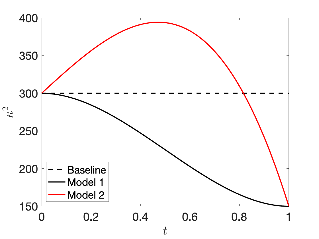
The outline is as follows: In the next subsection we introduce preliminaries and our notation. Section 2 is concerned with the general case of Gaussian measures on Hilbert spaces with fractional-order covariance operators. These outcomes are applied, in Section 3, to some first examples including the classical Whittle–Matérn model on a bounded domain $\mathcal{D}\subset\mathbb{R}^{d}$ and, in Section 4, to derive the results I.,II. for generalized Whittle–Matérn fields. In Section 5 the result II. is verified in two simulation studies for non-stationary random fields on the unit interval $\mathcal{D}=(0,1)$ . The manuscript concludes with a discussion in Section 6 and contains five Appendices A, B, C, D, F with auxiliary results and proofs.

1.2 Preliminaries and notation

If not specified otherwise, $(\,\cdot\,,\,\cdot\,)_{E}$ denotes the inner product on a Hilbert space $E$ , $\|\,\cdot\,\|_{E}$ the induced norm, $\operatorname{Id}_{E}$ the identity on $E$ , and $\mathcal{B}(E)$ the Borel $\sigma$ -algebra on $(E,\|\,\cdot\,\|_{E})$ , that is the smallest $\sigma$ -algebra containing all open sets. The scalar field $\mathbb{K}$ is either given by the real numbers $\mathbb{R}$ or the complex numbers $\mathbb{C}$ . The dual ${E}^{*}$ of $E$ is the space containing all continuous linear functionals $f\colon E\to\mathbb{K}$ , and we call $\langle\,\cdot\,,\,\cdot\,\rangle\colon{E}^{*}\times E\to\mathbb{K}$ , $\langle f,\psi\rangle:=f(\psi)$ the duality pairing between ${E}^{*}$ and $E$ .

The space of all bounded linear operators from $(E,(\,\cdot\,,\,\cdot\,)_{E})$ to a second Hilbert space $(F,(\,\cdot\,,\,\cdot\,)_{F})$ is denoted by $\mathcal{L}(E;F)$ . It is rendered a Banach space when equipped with the usual operator norm $\|T\|_{\mathcal{L}(E;F)}:=\sup_{\psi\in E\setminus\{0\}}\frac{\|T\psi\|_{F}}{\|\psi\|_{E}}$ . We call a linear operator $T\colon E\to F$ an isomorphism if $T\in\mathcal{L}(E;F)$ and $T^{-1}\in\mathcal{L}(F;E)$ , i.e., $T$ is bounded and has a bounded inverse. If $V$ is a vector space such that $E,F\subseteq V$ and if, in addition, $\operatorname{Id}_{V}|_{E}\in\mathcal{L}(E;F)$ , then $E$ is continuously embedded in $F$ and we write $(E,\|\,\cdot\,\|_{E})\hookrightarrow(F,\|\,\cdot\,\|_{F})$ . The notation $(E,\|\,\cdot\,\|_{E})\cong(F,\|\,\cdot\,\|_{F})$ indicates that $(E,\|\,\cdot\,\|_{E})$ and $(F,\|\,\cdot\,\|_{F})$ are isomorphic, i.e., $(E,\|\,\cdot\,\|_{E})\hookrightarrow(F,\|\,\cdot\,\|_{F})\hookrightarrow(E,\|\,\cdot\,\|_{E})$ . Whenever $E=F$ , we abbreviate $\mathcal{L}(E):=\mathcal{L}(E;E)$ , and this convention holds also for all other spaces of operators to be introduced. The subspaces $\mathcal{K}(E;F)\subseteq\mathcal{L}(E;F)$ and $\mathcal{L}_{2}(E;F)\subseteq\mathcal{L}(E;F)$ contain all compact operators and Hilbert–Schmidt operators, respectively. Note that $T\in\mathcal{L}(E;F)$ is compact if and only if it is the limit in $\mathcal{L}(E;F)$ of finite-rank operators, and $\mathcal{L}_{2}(E;F)$ is a Hilbert space with the inner product $(T,S)_{\mathcal{L}_{2}(E;F)}:=\sum_{j\in\mathbb{N}}(Te_{j},Se_{j})_{F}$ , where $\{e_{j}\}_{j\in\mathbb{N}}$ is any orthonormal basis for $E$ . The adjoint of $T\in\mathcal{L}(E;F)$ is identified with $T^{*}\in\mathcal{L}(F;E)$ (via the Riesz maps on $E$ and on $F$ ). An operator $T\in\mathcal{L}(E)$ is said to be orthogonal if $TT^{*}=T^{*}T=\operatorname{Id}_{E}$ , self-adjoint if $T=T^{*}$ , nonnegative definite if $(T\psi,\psi)_{E}\geq 0$ holds for all $\psi\in E$ , and positive definite if there exists a constant $\theta\in(0,\infty)$ such that $(T\psi,\psi)_{E}\geq\theta\|\psi\|_{E}^{2}$ for all $\psi\in E$ . A self-adjoint, nonnegative definite operator $T\in\mathcal{L}(E)$ has a finite trace if $\sum_{j\in\mathbb{N}}(Te_{j},e_{j})_{E}<\infty$ holds for an (or, equivalently, any) orthonormal basis $\{e_{j}\}_{j\in\mathbb{N}}$ of $E$ .

A (possibly unbounded) linear operator $A$ on $E$ with domain $\mathscr{D}(A)=\{\psi\in E:\|A\psi\|_{E}<\infty\}\subseteq E$ is denoted by $A\colon\mathscr{D}(A)\subseteq E\to E$ . It is closed if its graph $\mathscr{G}(A):={\{(x,Ax):x\in\mathscr{D}(A)\}}$ is closed with respect to the norm $\|(x,Ax)\|_{\mathscr{G}(A)}:=\|x\|_{E}+\|Ax\|_{E}$ and densely defined if $\mathscr{D}(A)$ is dense in $E$ .

Throughout this article, $(\Omega,\mathscr{F},\mathbb{P})$ is a complete probability space. For a Hilbert space $(E,(\,\cdot\,,\,\cdot\,)_{E})$ and $p\in[1,\infty)$ , $L_{p}(\Omega;E)$ denotes the space of (equivalence classes of) $E$ -valued, Bochner measurable random variables with finite $p$ -th moment, with norm $\|Z\|_{L_{p}(\Omega;E)}^{p}:=\int_{\Omega}\|Z(\omega)\|_{E}^{p}\,\mathrm{d}\mathbb{P}(\omega)$ . Further, $(\mathcal{X},d_{\mathcal{X}})$ is a connected, compact metric space of infinite cardinality, equipped with a strictly positive and finite Borel measure $\nu_{\mathcal{X}}$ , and $L_{2}(\mathcal{X},\nu_{\mathcal{X}})$ is the Hilbert space of (equivalence classes of) real-valued, Borel measurable, square-integrable functions on $\mathcal{X}$ , with $\|f\|_{L_{2}(\mathcal{X},\nu_{\mathcal{X}})}^{2}:=\int_{\mathcal{X}}|f(x)|^{2}\,\mathrm{d}\nu_{\mathcal{X}}(x)$ .

Finally, we write $\mathbb{R}_{+}:=(0,\infty)$ for the positive part of the real axis, $\mathbb{N}$ (or $\mathbb{N}_{0}$ ) for the set of positive (respectively, nonnegative) integers, and $\lfloor\,\cdot\,\rfloor$ (or $\lceil\,\cdot\,\rceil$ ) for the floor (respectively, ceiling) function.

2 Gaussian processes with fractional-order covariance operators

Throughout this section we let $(E,(\,\cdot\,,\,\cdot\,)_{E})$ be a separable Hilbert space over $\mathbb{R}$ with $\dim(E)=\infty$ . Furthermore, we assume that $\mu$ is a Gaussian measure on $E$ , i.e., for every $\psi\in E$ ,

\exists m_{\psi}\in\mathbb{R},\;\sigma_{\psi}^{2}\in\mathbb{R}_{+}:\quad\forall B\in\mathcal{B}(\mathbb{R})\quad\,\mu(\{\phi\in E:(\psi,\phi)_{E}\in B\})=\mathbb{P}(\{\omega\in\Omega:z_{\psi}(\omega)\in B\}),

where $z_{\psi}\colon\Omega\to\mathbb{R}$ is a random variable, which is either Gaussian distributed with mean $m_{\psi}$ and variance $\sigma_{\psi}^{2}$ , or concentrated at $m_{\psi}$ , i.e., $\mathbb{P}(\{\omega\in\Omega:z_{\psi}(\omega)=m_{\psi}\})=1$ . Then, there exist a vector $m\in E$ and a bounded linear operator $\mathcal{C}\colon E\to E$ such that, for all $\psi,\psi^{\prime}\in E$ ,

\textstyle(m,\psi)_{E}=\int_{E}(\phi,\psi)_{E}\,\mathrm{d}\mu(\phi),\qquad(\mathcal{C}\psi,\psi^{\prime})_{E}=\int_{E}(\psi,\phi-m)_{E}(\phi-m,\psi^{\prime})_{E}\,\mathrm{d}\mu(\phi).

(2.1)

The vector $m$ is the mean of the Gaussian measure $\mu$ and $\mathcal{C}$ is its covariance operator. One can show that $\mathcal{C}\colon E\to E$ is self-adjoint, nonnegative definite, and has a finite trace [5, Theorem 2.3.1]. Moreover, $\mu$ is uniquely determined by its mean $m$ and its covariance operator $\mathcal{C}$ , and we therefore write $\mu=\mathsf{N}(m,\mathcal{C})$ .

In this section we consider covariance operators of the form $\mathcal{C}=A^{-2\beta}$ , where $A$ is an unbounded linear operator on $E$ and $\beta\in\mathbb{R}_{+}$ . The main objectives of this section are to characterize for two given Gaussian measures $\mu:=\mathsf{N}\bigl(m,A^{-2\beta}\bigr)$ and $\widetilde{\mu}:=\mathsf{N}\bigl(\widetilde{m},\widetilde{A}^{-2\widetilde{\beta}}\bigr)$ the following:

I.

equivalence resp. orthogonality of $\mu$ and $\widetilde{\mu}$ , see Subsection 2.2, and
II.

uniform asymptotic optimality of linear predictions for $\mu$ based on the misspecified measure $\widetilde{\mu}$ when $E=L_{2}(\mathcal{X},\nu_{\mathcal{X}})$ , see Subsection 2.3.

To this end, in Subsection 2.1 we first specify our assumptions on $A$ and state two auxiliary results.

2.1 Hilbert space setting and some auxiliary results

In what follows, we assume that $A\colon\mathscr{D}(A)\subseteq E\to E$ is a densely defined, self-adjoint, positive definite linear operator, which has a compact inverse $A^{-1}\in\mathcal{K}(E)$ . In this case, $A\colon\mathscr{D}(A)\subseteq E\to E$ is closed and there exists an orthonormal basis $\{e_{j}\}_{j\in\mathbb{N}}$ for $E$ consisting of eigenvectors of $A$ , with corresponding positive eigenvalues $(\lambda_{j})_{j\in\mathbb{N}}$ accumulating only at $\infty$ . We assume that they are in non-decreasing order, $0<\lambda_{1}\leq\lambda_{2}\leq\ldots$ , and repeated according to multiplicity.

For $\beta\in[0,\infty)$ , the fractional power operator $A^{\beta}\colon\mathscr{D}\bigl(A^{\beta}\bigr)\subseteq E\to E$ can then be defined using the spectral expansion

A^{\beta}\psi:=\sum\limits_{j\in\mathbb{N}}\lambda_{j}^{\beta}(\psi,e_{j})_{E}\,e_{j},\qquad\psi\in\mathscr{D}\bigl(A^{\beta}\bigr)\subseteq E.

(2.2)

Note that, for all $r\in[0,\infty)$ , the domain of the operator $A^{\nicefrac{{r}}{{2}}}$ ,

\textstyle\dot{H}^{r}_{A}:=\mathscr{D}\bigl(A^{\nicefrac{{r}}{{2}}}\bigr),\quad\mathscr{D}\bigl(A^{\nicefrac{{r}}{{2}}}\bigr)=\Bigl\{\psi\in E:\|A^{\nicefrac{{r}}{{2}}}\psi\|_{E}^{2}=\sum\nolimits_{j\in\mathbb{N}}\lambda_{j}^{r}\,|(\psi,e_{j})_{E}|^{2}<\infty\Bigr\},

(2.3)

is itself a separable Hilbert space with respect to the inner product

\textstyle(\phi,\psi)_{r,A}:=(A^{\nicefrac{{r}}{{2}}}\phi,A^{\nicefrac{{r}}{{2}}}\psi)_{E}=\sum\nolimits_{j\in\mathbb{N}}\lambda_{j}^{r}\,(\phi,e_{j})_{E}(e_{j},\psi)_{E},

and the corresponding induced norm $\|\,\cdot\,\|_{r,A}$ . Here, $A^{0}:=\operatorname{Id}_{E}$ and $\dot{H}^{0}_{A}:=E$ . Recall that by definition the Cameron–Martin space of a Gaussian measure $\mu=\mathsf{N}(m,\mathcal{C})$ on $E$ (aka. the reproducing kernel Hilbert space of $\mathcal{C}$ ) is the image of $E$ under $\mathcal{C}^{\nicefrac{{1}}{{2}}}$ , endowed with the inner product $(\mathcal{C}^{-\nicefrac{{1}}{{2}}}\,\cdot\,,\mathcal{C}^{-\nicefrac{{1}}{{2}}}\,\cdot\,)_{E}$ , cf. [5, p. 44]. It consists of all elements $v\in E$ such that the measure $\mu_{v}(B):=\mu(B-v)$ is absolutely continuous with respect to $\mu$ (i.e., $\mu(B)=0\Rightarrow\mu_{v}(B)=0$ ). In particular, for $\mathcal{C}=A^{-2\beta}$ we obtain that

\mathcal{C}^{\nicefrac{{1}}{{2}}}(E)=A^{-\beta}(E)=\mathscr{D}\bigl(A^{\beta}\bigr)=\dot{H}^{2\beta}_{A},\qquad\|\mathcal{C}^{-\nicefrac{{1}}{{2}}}\,\cdot\,\|_{E}=\|\,\cdot\,\|_{2\beta,A}.

(2.4)

We let $\dot{H}^{-r}_{A}$ denote the dual space of $\dot{H}^{r}_{A}$ after identification via the inner product on $E$ which is continuously extended to a duality pairing. This means that for all $\phi\in E\subseteq\dot{H}^{-r}_{A}$ , $\psi\in\dot{H}^{r}_{A}\subseteq E$ , we have that $\langle\phi,\psi\rangle=(\phi,\psi)_{E}$ . It is an immediate consequence of these definitions that, for every $r,\vartheta\in\mathbb{R}$ , the fractional power operator $A^{\vartheta}\colon\dot{H}^{r}_{A}\to\dot{H}^{r-2\vartheta}_{A}$ is an isomorphism, possibly obtained as a continuous extension or restriction of $A^{\vartheta}\colon\mathscr{D}\bigl(A^{\vartheta}\bigr)=\dot{H}^{2\vartheta}_{A}\to\dot{H}^{0}_{A}=E$ . For ease of presentation, we postpone the technical proofs of the following two auxiliary results, Lemmas 2.1 and 2.2, to Appendix D.

Lemma 2.1.

(i)

Assume that there exists $\beta\in\mathbb{R}_{+}$ such that $\widetilde{A}^{\beta}A^{-\beta}\colon E\to E$ is an isomorphism and additionally $A^{-\beta}\widetilde{A}^{2\beta}A^{-\beta}-\operatorname{Id}_{E}\in\mathcal{L}_{2}(E)$ . Then, for every $\gamma\in[-\beta,\beta]$ , also the operator $\widetilde{A}^{\gamma}A^{-\gamma}$ is an isomorphism on $E$ and $A^{-\gamma}\widetilde{A}^{2\gamma}A^{-\gamma}-\operatorname{Id}_{E}\in\mathcal{L}_{2}(E)$ .
(ii)

Assume that there exists $\beta\in\mathbb{R}_{+}$ such that $\widetilde{A}^{\beta}A^{-\beta}\colon E\to E$ is an isomorphism and additionally $A^{-\beta}\widetilde{A}^{2\beta}A^{-\beta}-\operatorname{Id}_{E}\in\mathcal{K}(E)$ . Then, for every $\gamma\in[-\beta,\beta]$ , also the operator $\widetilde{A}^{\gamma}A^{-\gamma}$ is an isomorphism on $E$ and $A^{-\gamma}\widetilde{A}^{2\gamma}A^{-\gamma}-\operatorname{Id}_{E}\in\mathcal{K}(E)$ .

Lemma 2.2.

\mathfrak{N}_{\beta}:=\{n\in\mathbb{N}:n\leq\beta\}\cup\{\beta\}=\{1,\ldots,\lfloor\beta\rfloor\}\cup\{\beta\}.

(2.5)

(i)

$\widetilde{A}^{\gamma}A^{-\gamma}$ is an isomorphism on $E$ and $A^{-\gamma}\widetilde{A}^{2\gamma}A^{-\gamma}-\operatorname{Id}_{E}\in\mathcal{L}_{2}(E)$ for all $\gamma\in[-\beta,\beta]$ if and only if for all $\eta\in\mathfrak{N}_{\beta}$ there exist an orthogonal operator $U_{\eta}$ on $E$ and $S_{\eta}\in\mathcal{L}_{2}(E)$ such that $\operatorname{Id}_{E}+S_{\eta}$ is invertible on $E$ and $A^{\eta-1}\widetilde{A}A^{-\eta}=U_{\eta}(\operatorname{Id}_{E}+S_{\eta})$ .
(ii)

$\widetilde{A}^{\gamma}A^{-\gamma}$ is an isomorphism on $E$ and $A^{-\gamma}\widetilde{A}^{2\gamma}A^{-\gamma}-\operatorname{Id}_{E}\in\mathcal{K}(E)$ for all $\gamma\in[-\beta,\beta]$ if and only if for every $\eta\in\mathfrak{N}_{\beta}$ there exist an orthogonal operator $W_{\eta}$ on $E$ and $K_{\eta}\in\mathcal{K}(E)$ such that $\operatorname{Id}_{E}+K_{\eta}$ is invertible on $E$ and $A^{\eta-1}\widetilde{A}A^{-\eta}=W_{\eta}(\operatorname{Id}_{E}+K_{\eta})$ .
(iii)

The linear operator $\widetilde{A}^{\gamma}A^{-\gamma}\colon E\to E$ is an isomorphism for all $\gamma\in[-\beta,\beta]$ if and only if ${\widetilde{A}-A\in\mathcal{L}\bigl(\dot{H}^{2\eta}_{A};\dot{H}^{2(\eta-1)}_{A}\bigr)\cap\mathcal{L}\bigl(\dot{H}^{2\eta}_{\widetilde{A}};\dot{H}^{2(\eta-1)}_{\widetilde{A}}\bigr)}$ holds for every $\eta\in\{1,\beta\}$ .

2.2 Equivalence and orthogonality

Two probability measures $\mu,\widetilde{\mu}$ on $(E,\mathcal{B}(E))$ are said to be equivalent if, for all Borel sets $B\in\mathcal{B}(E)$ , $\mu(B)=0$ holds if and only if $\widetilde{\mu}(B)=0$ . In contrast, if there exists a Borel set $B\in\mathcal{B}(E)$ such that $\mu(B)=0$ and $\widetilde{\mu}(B)=1$ , then $\mu$ and $\widetilde{\mu}$ are said to be orthogonal. Two Gaussian measures $\mu,\widetilde{\mu}$ are either equivalent or orthogonal [5, Theorem 2.7.2]. As mentioned in the introduction, equivalence and orthogonality of Gaussian measures are important concepts in statistical theory. For example, a crucial first step in proving that a parameter $\theta$ of a Gaussian process (with corresponding Gaussian measure $\mu$ ) can be estimated consistently under infill asymptotics is often to define $\widetilde{\mu}$ as the Gaussian measure corresponding to the process with parameter $\widetilde{\theta}\neq\theta$ and to show that $\mu$ and $\widetilde{\mu}$ are orthogonal, see [41].

The following proposition provides necessary and sufficient conditions for equivalence of two Gaussian measures $\mu$ and $\widetilde{\mu}$ when they have fractional-order covariance operators.

Proposition 2.3.

Let $A\colon\mathscr{D}(A)\subseteq E\to E$ and $\widetilde{A}\colon\mathscr{D}(\widetilde{A})\subseteq E\to E$ be two densely defined, self-adjoint, positive definite linear operators with compact inverses on $E$ . In addition, let $\beta\in[1,\infty)$ , $\widetilde{\beta}\in\mathbb{R}_{+}$ be such that $A^{-2\beta}$ and $\widetilde{A}^{-2\widetilde{\beta}}$ have finite traces on $E$ , let $m,\widetilde{m}\in E$ , and define $\delta:=\nicefrac{{\widetilde{\beta}}}{{\beta}}\in\mathbb{R}_{+}$ . The Gaussian measures $\mu=\mathsf{N}\bigl(m,A^{-2\beta}\bigr)$ and $\widetilde{\mu}=\mathsf{N}\bigl(\widetilde{m},\widetilde{A}^{-2\widetilde{\beta}}\bigr)$ are either equivalent or orthogonal. They are equivalent if and only if the following two conditions are satisfied:

(a)

the difference of the means satisfies $m-\widetilde{m}\in\dot{H}^{2\beta}_{A}$ ;
(b)

for all $\eta\in\mathfrak{N}_{\beta}$ , where $\mathfrak{N}_{\beta}$ is defined as in (2.5), there exist an orthogonal operator $U_{\eta}\in\mathcal{L}(E)$ and $S_{\eta}\in\mathcal{L}_{2}(E)$ such that $A^{\eta-1}\widetilde{A}^{\delta}A^{-\eta}=U_{\eta}(\operatorname{Id}_{E}+S_{\eta})$ and $\operatorname{Id}_{E}+S_{\eta}$ is invertible on $E$ .

Condition (b) is in particular satisfied, whenever

\widetilde{A}^{\delta}-A\in\mathcal{L}_{2}\bigl(\dot{H}^{2\eta}_{A};\dot{H}^{2(\eta-1)}_{A}\bigr)\quad\forall\eta\in\mathfrak{N}_{\beta},\quad\text{and}\quad\widetilde{A}^{\delta}-A\in\mathcal{L}\bigl(\dot{H}^{2\delta\eta}_{\widetilde{A}};\dot{H}^{2\delta(\eta-1)}_{\widetilde{A}}\bigr)\quad\forall\eta\in\{1,\beta\}.

Proof.

In order to derive the equivalence statement, we apply the Feldman–Hájek theorem, see Theorem B.1 in Appendix B: $\mu$ and $\widetilde{\mu}$ are equivalent if and only if

(i)

the Cameron–Martin spaces $\dot{H}^{2\beta}_{A}$ and $\dot{H}^{2\widetilde{\beta}}_{\widetilde{A}}$ (see (2.4)) are norm equivalent Hilbert spaces;
(ii)

the difference of the means satisfies $m-\widetilde{m}\in\dot{H}^{2\beta}_{A}$ ; and
(iii)

the operator $A^{-\beta}\widetilde{A}^{2\widetilde{\beta}}A^{-\beta}-\operatorname{Id}_{E}$ is a Hilbert–Schmidt operator on $E$ .

It remains to prove that conditions (i) and (iii) are equivalent to condition (b) of the proposition. By Lemma 2.2 (i), applied for the pair of operators $A,\widetilde{A}^{\delta}$ , (b) is equivalent to $(\widetilde{A}^{\delta})^{\gamma}A^{-\gamma}=\widetilde{A}^{\delta\gamma}A^{-\gamma}$ being an isomorphism on $E$ and $A^{-\gamma}(\widetilde{A}^{\delta})^{2\gamma}A^{-\gamma}-\operatorname{Id}_{E}=A^{-\gamma}\widetilde{A}^{2\delta\gamma}A^{-\gamma}-\operatorname{Id}_{E}\in\mathcal{L}_{2}(E)$ for $\gamma\in[-\beta,\beta]$ . The choice $\gamma:=\beta$ shows that $\dot{H}^{2\beta}_{A}\cong\dot{H}^{2\widetilde{\beta}}_{\widetilde{A}}$ and $A^{-\beta}\widetilde{A}^{2\widetilde{\beta}}A^{-\beta}-\operatorname{Id}_{E}\in\mathcal{L}_{2}(E)$ , i.e., (i) and (iii) hold. Conversely, if (i) and (iii) are satisfied, then by Lemma 2.1 (i) we obtain that $\widetilde{A}^{\delta\gamma}A^{-\gamma}$ is an isomorphism on $E$ and $A^{-\gamma}\widetilde{A}^{2\delta\gamma}A^{-\gamma}-\operatorname{Id}_{E}\in\mathcal{L}_{2}(E)$ for all $\gamma\in[-\beta,\beta]$ . Thus, (b) is satisfied by Lemma 2.2 (i).

Since $A^{\eta-1}\widetilde{A}^{\delta}A^{-\eta}-\operatorname{Id}_{E}=A^{\eta-1}(\widetilde{A}^{\delta}-A)A^{-\eta}$ , the condition $\widetilde{A}^{\delta}-A\in\mathcal{L}_{2}\bigl(\dot{H}^{2\eta}_{A};\dot{H}^{2(\eta-1)}_{A}\bigr)$ implies that $S_{\eta}:=A^{\eta-1}\widetilde{A}^{\delta}A^{-\eta}-\operatorname{Id}_{E}\in\mathcal{L}_{2}(E)$ for all $\eta\in\mathfrak{N}_{\beta}$ . Furthermore, if also $\widetilde{A}^{\delta}-A$ is in $\mathcal{L}\bigl(\dot{H}^{2\delta\eta}_{\widetilde{A}};\dot{H}^{2\delta(\eta-1)}_{\widetilde{A}}\bigr)=\mathcal{L}\bigl(\dot{H}^{2\eta}_{\widetilde{A}^{\delta}};\dot{H}^{2(\eta-1)}_{\widetilde{A}^{\delta}}\bigr)$ for $\eta\in\{1,\beta\}$ , then by Lemma 2.2 (iii) (applied for the pair of operators $A,\widetilde{A}^{\delta}$ ) $\widetilde{A}^{\delta\gamma}A^{-\gamma}$ is an isomorphism on $E$ for all $\gamma\in[-\beta,\beta]$ . Therefore, $\operatorname{Id}_{E}+S_{\eta}=A^{\eta-1}\widetilde{A}^{-\delta(\eta-1)}\widetilde{A}^{\delta\eta}A^{-\eta}$ is invertible on $E$ , and (b) holds for the choice $U_{\eta}=\operatorname{Id}_{E}$ for all $\eta\in\mathfrak{N}_{\beta}$ . ∎

By applying Proposition 2.3 for the pair of measures $\widehat{\mu}:=\mathsf{N}\bigl(m,\widehat{A}^{-2}\bigr)$ and $\widetilde{\mu}=\mathsf{N}\bigl(\widetilde{m},\widetilde{A}^{-2\widetilde{\beta}}\bigr)$ , where ${\widehat{A}:=A^{\beta}}$ , we also obtain a corresponding result which includes the case that $\beta\in(0,1)$ .

Corollary 2.4.

Under the assumptions of Proposition 2.3 on $m,\widetilde{m},A,\widetilde{A}$ , and for $\beta,\widetilde{\beta}\in\mathbb{R}_{+}$ such that $A^{-2\beta}\!,\widetilde{A}^{-2\widetilde{\beta}}$ have finite traces, the Gaussian measures $\mu=\mathsf{N}\bigl(m,A^{-2\beta}\bigr)$ and $\widetilde{\mu}=\mathsf{N}\bigl(\widetilde{m},\widetilde{A}^{-2\widetilde{\beta}}\bigr)$ are equivalent if and only if (a) $m-\widetilde{m}\in\dot{H}^{2\beta}_{A}$ and (b) there exist an orthogonal operator $U\in\mathcal{L}(E)$ and $S\in\mathcal{L}_{2}(E)$ such that $\widetilde{A}^{\widetilde{\beta}}A^{-\beta}=U(\operatorname{Id}_{E}+S)$ and $\operatorname{Id}_{E}+S$ is invertible on $E$ .

Remark 2.5.

At first glance, condition (b) of Corollary 2.4 seems easier compared to (b) of Proposition 2.3. We note that the advantage of the latter is that, whenever $\beta=\widetilde{\beta}$ , it is formulated solely in terms of the base operator $\widetilde{A}$ (and not of powers thereof).

2.3 Uniformly asymptotically optimal linear prediction

Throughout this subsection, we let $(\mathcal{X},d_{\mathcal{X}})$ be a connected, compact metric space with positive, finite Borel measure $\nu_{\mathcal{X}}$ (see Subsection 1.2) and we consider $E=L_{2}(\mathcal{X},\nu_{\mathcal{X}})$ . Suppose that $Z\colon\mathcal{X}\times\Omega\to\mathbb{R}$ is a square-integrable random field with mean $m\in L_{2}(\mathcal{X},\nu_{\mathcal{X}})$ and covariance operator $A^{-2\beta}$ , where $A\colon\mathscr{D}(A)\subseteq L_{2}(\mathcal{X},\nu_{\mathcal{X}})\to L_{2}(\mathcal{X},\nu_{\mathcal{X}})$ is as described in Subsection 2.1. Let $\mu=\mathsf{N}\bigl(m,A^{-2\beta}\bigr)$ be the Gaussian measure corresponding to $Z$ and define $\mathsf{E}[\,\cdot\,]$ as the expectation under $\mu$ . That is, for a random variable $Y\colon\Omega\to L_{2}(\mathcal{X},\nu_{\mathcal{X}})$ with distribution $\mu$ and a Borel measurable function $g\colon L_{2}(\mathcal{X},\nu_{\mathcal{X}})\to\mathbb{R}$ , we have that $m=\mathsf{E}[Y]:=\int_{L_{2}(\mathcal{X},\nu_{\mathcal{X}})}y\,\mathrm{d}\mu(y)$ and, provided that the integral $\int_{L_{2}(\mathcal{X},\nu_{\mathcal{X}})}g(y)\,\mathrm{d}\mu(y)$ exists, we define $\mathsf{E}[g(Y)]:=\int_{L_{2}(\mathcal{X},\nu_{\mathcal{X}})}g(y)\,\mathrm{d}\mu(y)$ .

To characterize optimal linear prediction for $Z$ , we introduce the centered process $Z^{0}:=Z-m$ and the vector space $\mathcal{Z}^{0}$ consisting of all linear combinations of the form ${\alpha_{1}Z^{0}(x_{1})+\ldots+\alpha_{K}Z^{0}(x_{K})}$ , where $K\in\mathbb{N}$ and $\alpha_{j}\in\mathbb{R}$ , $x_{j}\in\mathcal{X}$ for all $j\in\{1,\ldots,K\}$ . We then define the Hilbert space $\mathcal{H}^{0}$ as the closure of $\mathcal{Z}^{0}$ with respect to the norm $\|\,\cdot\,\|_{\mathcal{H}^{0}}$ induced by the $L_{2}(\Omega,\mathbb{P})$ inner product,

\textstyle\biggl(\sum\limits_{j=1}^{K}\alpha_{j}Z^{0}(x_{j}),\,\sum\limits_{k=1}^{K^{\prime}}\alpha_{k}^{\prime}Z^{0}(x_{k}^{\prime})\biggr)_{\mathcal{H}^{0}}:=\sum\limits_{j=1}^{K}\sum\limits_{k=1}^{K^{\prime}}\alpha_{j}\alpha_{k}^{\prime}\mathsf{E}\bigl[Z^{0}(x_{j})Z^{0}(x_{k}^{\prime})\bigr].

Since any observation or linear predictor of $Z$ can be represented as $h=c+h^{0}$ for $c\in\mathbb{R}$ and $h^{0}\in\mathcal{H}^{0}$ , we introduce the Hilbert space $\mathcal{H}$ as the direct sum $\mathcal{H}:=\mathbb{R}\oplus\mathcal{H}^{0}$ equipped with the graph norm $\|h\|_{\mathcal{H}}^{2}=|c|^{2}+\|h^{0}\|_{\mathcal{H}^{0}}^{2}$ . Suppose now that we want to predict $h\in\mathcal{H}$ based on a set of observations $\{y_{nj}\}_{j=1}^{n}$ , where $y_{nj}=c_{nj}+y_{nj}^{0}$ for $c_{nj}\in\mathbb{R}$ and $y_{nj}^{0}\in\mathcal{H}^{0}$ . Then, the best linear predictor (aka. kriging predictor, see e.g. [36, Section 1.2] and [26, Section 2]) of $h$ based on these observations is the $\mathcal{H}$ -orthogonal projection of $h$ onto the subspace

\textstyle\mathcal{H}_{n}:=\mathbb{R}\oplus\mathcal{H}^{0}_{n}=\biggl\{\alpha_{0}+\sum\limits_{j=1}^{n}\alpha_{j}y_{nj}^{0}:\alpha_{0},\ldots,\alpha_{n}\in\mathbb{R}\biggr\},\qquad\mathcal{H}^{0}_{n}:=\operatorname{span}\bigl\{y_{nj}^{0}\bigr\}_{j=1}^{n}.

(2.6)

That is, the best linear predictor $h_{n}\in\mathcal{H}_{n}$ satisfies

\textstyle(h_{n}-h,g_{n})_{\mathcal{H}}=0\quad\forall g_{n}\in\mathcal{H}_{n},\quad\;\;\text{and}\qquad\|h_{n}-h\|_{\mathcal{H}}=\inf_{g_{n}\in\mathcal{H}_{n}}\|g_{n}-h\|_{\mathcal{H}}.

(2.7)

The question is now what happens if we replace $h_{n}$ with another linear predictor $\widetilde{h}_{n}$ , which is computed based on an incorrect model. Specifically, let $\widetilde{\mu}=\mathsf{N}\bigl(\widetilde{m},\widetilde{A}^{-2\widetilde{\beta}}\bigr)$ be a second Gaussian measure with corresponding expectation operator $\widetilde{\mathsf{E}}[\,\cdot\,]$ , and let $\widetilde{h}_{n}$ be the best linear predictor for the model $\widetilde{\mu}$ . We are interested in the quality of $\widetilde{h}_{n}$ compared to $h_{n}$ asymptotically as $n\to\infty$ . For this purpose, we assume that the set of observations $\bigl\{\{y_{nj}\}_{j=1}^{n}:n\in\mathbb{N}\bigr\}$ yields $\mu$ -consistent kriging prediction, i.e.,

\lim\limits_{n\to\infty}\mathsf{E}\bigl[(h_{n}-h)^{2}\bigr]=\lim\limits_{n\to\infty}\|h_{n}-h\|_{\mathcal{H}}^{2}=0,

(2.8)

and we let $\mathcal{S}^{\mu}_{\mathrm{adm}}$ denote the set of all admissible sequences of observations which provide $\mu$ -consistent kriging prediction:

\begin{split}\mathcal{S}^{\mu}_{\mathrm{adm}}:=\bigl\{\{\mathcal{H}_{n}\}_{n\in\mathbb{N}}\;\bigl|\;&\forall n\in\mathbb{N}:\mathcal{H}_{n}\text{ is as in \eqref{eq:def:cHn} with}\,\dim(\mathcal{H}_{n}^{0})=n,\\ &\forall h\in\mathcal{H}:\{h_{n}\}_{n\in\mathbb{N}}\text{ defined by \eqref{eq:def:hn} satisfy \eqref{eq:ass:Hn-dense}}\bigr\}.\end{split}

(2.9)

By combining the results of Lemmas 2.1 and 2.2 with [26, Theorem 3.8] we obtain the following result on uniformly asymptotically optimal linear prediction when misspecifying $\mu$ by $\widetilde{\mu}$ .

Proposition 2.6.

Let $h_{n},\widetilde{h}_{n}$ denote the best linear predictors of $h\in\mathcal{H}$ based on $\mathcal{H}_{n}$ and the measures ${\mu=\mathsf{N}\bigl(m,A^{-2\beta}\bigr)}$ and $\widetilde{\mu}=\mathsf{N}\bigl(\widetilde{m},\widetilde{A}^{-2\widetilde{\beta}}\bigr)$ , respectively. Here, assume that $m,\widetilde{m}\in L_{2}(\mathcal{X},\nu_{\mathcal{X}})$ , $A\colon\mathscr{D}(A)\subseteq L_{2}(\mathcal{X},\nu_{\mathcal{X}})\to L_{2}(\mathcal{X},\nu_{\mathcal{X}})$ and $\widetilde{A}\colon\mathscr{D}(\widetilde{A})\subseteq L_{2}(\mathcal{X},\nu_{\mathcal{X}})\to L_{2}(\mathcal{X},\nu_{\mathcal{X}})$ are densely defined, self-adjoint, positive definite linear operators with compact inverses on $L_{2}(\mathcal{X},\nu_{\mathcal{X}})$ . In addition, $\beta,\widetilde{\beta}\in\mathbb{R}_{+}$ are such that $A^{-2\beta}$ and $\widetilde{A}^{-2\widetilde{\beta}}$ have finite traces on $L_{2}(\mathcal{X},\nu_{\mathcal{X}})$ and $\delta:=\nicefrac{{\widetilde{\beta}}}{{\beta}}$ .

Set $\mathcal{H}_{-n}:=\bigl\{h\in\mathcal{H}:\mathsf{E}\bigl[(h_{n}-h)^{2}\bigr]>0\bigr\}$ . Any of the following four asymptotic statements,

	$\displaystyle\lim_{n\to\infty}\sup_{h\in\mathcal{H}_{-n}}\frac{\mathsf{E}\bigl[(\widetilde{h}_{n}-h)^{2}\bigr]}{\mathsf{E}\bigl[(h_{n}-h)^{2}\bigr]}$	$\displaystyle=1,$	$\displaystyle\lim_{n\to\infty}\sup_{h\in\mathcal{H}_{-n}}\frac{\widetilde{\mathsf{E}}\bigl[(h_{n}-h)^{2}\bigr]}{\widetilde{\mathsf{E}}\bigl[(\widetilde{h}_{n}-h)^{2}\bigr]}$	$\displaystyle=1,$		(2.10)
	$\displaystyle\lim_{n\to\infty}\sup_{h\in\mathcal{H}_{-n}}\left\|\frac{\widetilde{\mathsf{E}}\bigl[(h_{n}-h)^{2}\bigr]}{\mathsf{E}\bigl[(h_{n}-h)^{2}\bigr]}-c\right\|$	$\displaystyle=0,$	$\displaystyle\;\;\;\lim_{n\to\infty}\sup_{h\in\mathcal{H}_{-n}}\left\|\frac{\mathsf{E}\bigl[(\widetilde{h}_{n}-h)^{2}\bigr]}{\widetilde{\mathsf{E}}\bigl[(\widetilde{h}_{n}-h)^{2}\bigr]}-\frac{1}{c}\right\|$	$\displaystyle=0,$		(2.11)

holds for all $\{\mathcal{H}_{n}\}_{n\in\mathbb{N}}\in\mathcal{S}^{\mu}_{\mathrm{adm}}$ (and in (2.11) for some $c\in\mathbb{R}_{+}$ ) if and only if

(a)

the difference of the means satisfies $m-\widetilde{m}\in\dot{H}^{2\beta}_{A}$ ;
(b)

there exist $c\in\mathbb{R}_{+}$ , an orthogonal operator $W$ on $L_{2}(\mathcal{X},\nu_{\mathcal{X}})$ , and $K\in\mathcal{K}(L_{2}(\mathcal{X},\nu_{\mathcal{X}}))$ such that $c^{\nicefrac{{1}}{{2}}}\widetilde{A}^{\widetilde{\beta}}A^{-\beta}=W(\operatorname{Id}_{L_{2}(\mathcal{X},\nu_{\mathcal{X}})}+K)$ and $\operatorname{Id}_{L_{2}(\mathcal{X},\nu_{\mathcal{X}})}+K$ is invertible.

In this case, the constant $c\in\mathbb{R}_{+}$ in condition I.(b) coincides with that in (2.11).

II.

For $\beta\in[1,\infty)$ , condition I.(b) is equivalent to requiring that there exists $c\in\mathbb{R}_{+}$ such that for all $\eta\in\mathfrak{N}_{\beta}$ , where $\mathfrak{N}_{\beta}$ is defined as in (2.5), there exist an orthogonal operator $W_{\eta}$ on $L_{2}(\mathcal{X},\nu_{\mathcal{X}})$ and ${K_{\eta}\in\mathcal{K}(L_{2}(\mathcal{X},\nu_{\mathcal{X}}))}$ such that $c^{\frac{1}{2\beta}}A^{\eta-1}\widetilde{A}^{\delta}A^{-\eta}=W_{\eta}(\operatorname{Id}_{L_{2}(\mathcal{X},\nu_{\mathcal{X}})}+K_{\eta})$ and $\operatorname{Id}_{L_{2}(\mathcal{X},\nu_{\mathcal{X}})}+K_{\eta}$ is invertible on $L_{2}(\mathcal{X},\nu_{\mathcal{X}})$ . This is satisfied, whenever the following holds:

\forall\eta\in\mathfrak{N}_{\beta}:\quad c^{\frac{1}{2\beta}}\widetilde{A}^{\delta}-A\in\mathcal{K}\bigl(\dot{H}^{2\eta}_{A};\dot{H}^{2(\eta-1)}_{A}\bigr)\cap\mathcal{L}\bigl(\dot{H}^{2\delta\eta}_{\widetilde{A}};\dot{H}^{2\delta(\eta-1)}_{\widetilde{A}}\bigr).

Proof.

By [26, Theorem 3.8 and Lemma B.1] any of the assertions in (2.10) or (2.11) holds for every $\{\mathcal{H}_{n}\}_{n\in\mathbb{N}}\in\mathcal{S}^{\mu}_{\mathrm{adm}}$ and for some constant $c\in\mathbb{R}_{+}$ if and only if

(i)

the Cameron–Martin spaces $\dot{H}^{2\beta}_{A}$ and $\dot{H}^{2\widetilde{\beta}}_{\widetilde{A}}$ are norm equivalent Hilbert spaces;
(ii)

the difference of the means satisfies $m-\widetilde{m}\in\dot{H}^{2\beta}_{A}$ ; and
(iii)

$A^{-\beta}\widetilde{A}^{2\widetilde{\beta}}A^{-\beta}-c^{-1}\operatorname{Id}_{E}=c^{-1}\bigl(A^{-\beta}\bigl(c\widetilde{A}^{2\widetilde{\beta}}\bigr)A^{-\beta}-\operatorname{Id}_{E}\bigr)$ is compact on $E$ .

The proof for II., when $\beta\in[1,\infty)$ , can then be completed as in the proof of Proposition 2.3, namely by using Lemma 2.1 (ii) and Lemma 2.2 (ii)/(iii) for the pair of operators $A$ and $c^{\frac{1}{2\beta}}\widetilde{A}^{\delta}$ . Finally, the general statement I. for $\beta,\widetilde{\beta}\in\mathbb{R}_{+}$ follows similarly as Corollary 2.4. ∎

3 Some explicit choices for the base operators

In this section we illustrate the abstract results of Section 2 by two first examples before discussing their implications for generalized Whittle–Matérn fields in the next section: In Subsection 3.1 we consider the case that the base operators $A$ and $\widetilde{A}$ diagonalize with respect to the same eigenbasis $\{e_{j}\}_{j\in\mathbb{N}}$ for $E$ . This setting applies to classical Whittle–Matérn fields with constant coefficients, which solve SPDEs of the form (1.2) on a bounded domain $\mathcal{D}\subset\mathbb{R}^{d}$ . We subsequently discuss this example in Subsection 3.2.

3.1 Operators with the same eigenbasis

We note that the scope for applications of the following corollary is considerably wider than the classical Whittle–Matérn class discussed in Subsection 3.2. For instance, it can be used for periodic random fields on $\mathcal{X}=[0,1]^{d}$ as considered by Stein [35], random fields on the sphere $\mathcal{X}=\mathbb{S}^{2}$ defined via the spherical harmonics, see e.g. [21] and [26, Section 6.3], or more generally Gaussian processes on compact Riemannian manifolds defined via the eigenfunctions of the Laplace–Beltrami operator [10].

Corollary 3.1.

Let $A\colon\mathscr{D}(A)\subseteq E\to E$ and $\widetilde{A}\colon\mathscr{D}(\widetilde{A})\subseteq E\to E$ be two densely defined, self-adjoint, positive definite linear operators with compact inverses on $E$ . In addition, assume that $A$ and $\widetilde{A}$ diagonalize with respect to the same eigenbasis $\{e_{j}\}_{j\in\mathbb{N}}$ for $E$ , i.e., there exist corresponding eigenvalues $\mathbb{R}_{+}\ni\lambda_{j},\widetilde{\lambda}_{j}\to\infty$ (as $j\to\infty$ ) such that $Ae_{j}=\lambda_{j}e_{j}$ and $\widetilde{A}e_{j}=\widetilde{\lambda}_{j}e_{j}$ for all $j\in\mathbb{N}$ . Let $m,\widetilde{m}\in E$ , and assume that $\beta,\delta\in\mathbb{R}_{+}$ are such that $A^{-2\beta}$ and $\widetilde{A}^{-2\delta\beta}$ have finite traces on $E$ . Then, the Gaussian measures $\mu=\mathsf{N}\bigl(m,A^{-2\beta}\bigr)$ and $\widetilde{\mu}=\mathsf{N}\bigl(\widetilde{m},\widetilde{A}^{-2\delta\beta}\bigr)$ satisfy the following:

I.

The Cameron–Martin spaces for $\mu$ and $\widetilde{\mu}$ are isomorphic, with equivalent norms, if and only if there exist $c_{-},c_{+}\in\mathbb{R}_{+}$ such that $c_{j}:=\widetilde{\lambda}_{j}^{\delta}\lambda_{j}^{-1}\in[c_{-},c_{+}]$ for all $j\in\mathbb{N}$ .
II.

The measures $\mu$ and $\widetilde{\mu}$ are equivalent if and only if $m-\widetilde{m}\in\dot{H}^{2\beta}_{A}$ and $\sum_{j\in\mathbb{N}}(c_{j}-1)^{2}<\infty$ .
III.

Any of the four assertions in (2.10), (2.11) holds for all $\{\mathcal{H}_{n}\}_{n\in\mathbb{N}}\in\mathcal{S}^{\mu}_{\mathrm{adm}}$ and in (2.11) for some $c\in\mathbb{R}_{+}$ if and only if $m-\widetilde{m}\in\dot{H}^{2\beta}_{A}$ and $\lim_{j\to\infty}c_{j}=\hat{c}$ for some $\hat{c}\in\mathbb{R}_{+}$ . Then, $c=\hat{c}^{-2\beta}$ .

Proof.

Define $c_{-}:=\inf_{j\in\mathbb{N}}\widetilde{\lambda}_{j}^{\delta}\lambda_{j}^{-1}\in[0,\infty)$ and $c_{+}:=\sup_{j\in\mathbb{N}}\widetilde{\lambda}_{j}^{\delta}\lambda_{j}^{-1}\in(0,\infty]$ . Then, we obtain that $\|\phi\|_{2\delta\beta,\widetilde{A}}\leq c_{+}^{\beta}\|\phi\|_{2\beta,A}$ and $c_{-}^{\beta}\|\psi\|_{2\beta,A}\leq\|\psi\|_{2\delta\beta,\widetilde{A}}$ for all $\phi\in\dot{H}^{2\beta}_{A}$ and $\psi\in\dot{H}^{2\delta\beta}_{\widetilde{A}}$ . Therefore, the Cameron–Martin spaces for $\mu$ and $\widetilde{\mu}$ , see (2.4), are isomorphic if and only if $c_{-}>0$ and $c_{+}<\infty$ .

Note that $(c_{j})_{j\in\mathbb{N}}\subset\mathbb{R}_{+}$ and $\sum_{j\in\mathbb{N}}(c_{j}-1)^{2}<\infty$ imply that $0<c_{-}\leq c_{j}\leq c_{+}<\infty$ for all $j\in\mathbb{N}$ . Thus, II. follows from I. and the Feldman–Hájek theorem, Theorem B.1, since by the mean value theo-

rem for $t\mapsto t^{2\beta}$ , $\|A^{-\beta}\widetilde{A}^{2\delta\beta}A^{-\beta}-\operatorname{Id}_{E}\|_{\mathcal{L}_{2}(E)}^{2}=\sum_{j\in\mathbb{N}}\bigl(c_{j}^{2\beta}-1\bigr)^{2}=4\beta^{2}\sum_{j\in\mathbb{N}}\xi_{j}^{2(2\beta-1)}(c_{j}-1)^{2}$ , where $(\xi_{j})_{j\in\mathbb{N}}$ satisfy that $\xi_{j}\in[\min\{c_{j},1\},\max\{c_{j},1\}]\subseteq[\min\{c_{-},1\},\max\{c_{+},1\}]$ for all $j\in\mathbb{N}$ .

Finally, the assertion III. has already been observed in [26, Corollary 5.1]; there formulated in terms of the ratio $\widetilde{\gamma}_{j}/\gamma_{j}\to c$ (as $j\to\infty$ ) of the eigenvalues $(\widetilde{\gamma}_{j})_{j\in\mathbb{N}}$ and $(\gamma_{j})_{j\in\mathbb{N}}$ of the covariance operators $\widetilde{\mathcal{C}}=\widetilde{A}^{-2\delta\beta}$ and $\mathcal{C}=A^{-2\beta}$ . Thus, $\widetilde{\gamma}_{j}/\gamma_{j}=\widetilde{\lambda}_{j}^{-2\delta\beta}\lambda_{j}^{2\beta}=c_{j}^{-2\beta}$ and the claim follows. ∎

Remark 3.2.

Note that for $\mu=\mathsf{N}\bigl(0,A^{-2\beta}\bigr)$ and $\widetilde{\mu}=\mathsf{N}\bigl(0,\widetilde{A}^{-2\delta\beta}\bigr)$ the conditions in all parts of Corollary 3.1 are independent of $\beta\in\mathbb{R}_{+}$ . This implies that once a property (equivalent Cameron–Martin spaces, equivalence of measures, or uniformly asymptotically optimal linear prediction) is established for $\mu,\widetilde{\mu}$ and a fixed $\beta=\beta_{0}\in\mathbb{R}_{+}$ , it follows also for all other meaningful values of $\beta\in\mathbb{R}_{+}$ so that $A^{-2\beta}\!,\widetilde{A}^{-2\delta\beta}$ have finite traces. Thus, in the case that $A$ and $\widetilde{A}$ diagonalize with respect to the same eigenbasis, besides concluding the corresponding property for $\beta\leq\beta_{0}$ (by means of Lemma 2.1) one obtains it also for $\beta>\beta_{0}$ . This observation holds even for more general base operators $A,\widetilde{A}$ . Specifically, if their fractional powers commute, i.e., $\mathscr{D}(\widetilde{A}^{\vartheta}A^{r})=\mathscr{D}(A^{r}\widetilde{A}^{\vartheta})$ and $\widetilde{A}^{\vartheta}A^{r}\psi=A^{r}\widetilde{A}^{\vartheta}\psi$ for all $r,\vartheta\in\mathbb{R}$ and $\psi\in\mathscr{D}(\widetilde{A}^{\vartheta}A^{r})$ , then the operators $A^{\eta-1}\widetilde{A}^{\delta}A^{-\eta}$ , $\eta\in\mathfrak{N}_{\beta}$ , appearing in the conditions of Propositions 2.3 and 2.6 simplify to $\widetilde{A}^{\delta}A^{-1}$ and the conditions become independent of $\beta\in[1,\infty)$ .

3.2 Whittle–Matérn operators with constant coefficients

We now discuss classical Whittle–Matérn fields solving the SPDE (1.2) on a bounded domain. To this end, let $\emptyset\neq\mathcal{D}\subset\mathbb{R}^{d}$ be a connected, bounded and open domain, with Lipschitz boundary $\partial\mathcal{D}$ . Further,

Lv:=\bigl(-\Delta+\kappa^{2}\bigr)v,\qquad v\in\mathscr{D}(L):=H^{2}(\mathcal{D})\cap H^{1}_{0}(\mathcal{D}),

(3.1)

is the negative Laplacian, shifted by $\kappa^{2}\in[0,\infty)$ and augmented with homogeneous Dirichlet boundary conditions, see Appendix A.3. By Proposition 4.2 $L^{-2\beta}$ has a finite trace if and only if $\beta\in(\nicefrac{{d}}{{4}},\infty)$ . Recall that for the SPDE (1.2) on $\mathbb{R}^{d}$ this condition corresponds to a positive smoothness parameter $\nu=2\beta-\nicefrac{{d}}{{2}}\in\mathbb{R}_{+}$ . For two classical Whittle–Matérn fields with parameters $(\beta,\tau,\kappa)$ and $(\widetilde{\beta},\widetilde{\tau},\widetilde{\kappa})$ , where $\tau,\widetilde{\tau}$ scale the variances of the fields, cf. (5.1), we obtain the following result from Corollary 3.1.

Corollary 3.3.

Let $d\in\mathbb{N}$ , $\beta,\widetilde{\beta}\in(\nicefrac{{d}}{{4}},\infty)$ , $\tau,\widetilde{\tau}\in\mathbb{R}_{+}$ , and let $L,\widetilde{L}$ be defined as in (3.1) with shift parameters $\kappa^{2}\in[0,\infty)$ and $\widetilde{\kappa}^{2}\in[0,\infty)$ , respectively. Assume that $m,\widetilde{m}\in L_{2}(\mathcal{D})$ and consider the Gaussian measures $\mu=\mathsf{N}\bigl(m,\tau^{-2}L^{-2\beta}\bigr)$ and $\widetilde{\mu}=\mathsf{N}\bigl(\widetilde{m},\widetilde{\tau}^{-2}\widetilde{L}^{-2\widetilde{\beta}}\bigr)$ on the Hilbert space $L_{2}(\mathcal{D})$ .

I.

The Cameron–Martin spaces for $\mu,\widetilde{\mu}$ are isomorphic, with equivalent norms, if and only if $\beta=\widetilde{\beta}$ .
II.

In dimension $d\leq 3$ , $\mu$ and $\widetilde{\mu}$ are equivalent if and only if $\beta=\widetilde{\beta}$ , $\tau=\widetilde{\tau}$ and $m-\widetilde{m}\in\dot{H}^{2\beta}_{L}$ . In dimension $d\geq 4$ , $\mu$ and $\widetilde{\mu}$ are equivalent if and only if $\beta=\widetilde{\beta}$ , $\tau=\widetilde{\tau}$ , $m-\widetilde{m}\in\dot{H}^{2\beta}_{L}$ and $\kappa^{2}=\widetilde{\kappa}^{2}$ .
III.

In every dimension $d\in\mathbb{N}$ , any of the four assertions in (2.10), (2.11) holds for every sequence $\{\mathcal{H}_{n}\}_{n\in\mathbb{N}}\in\mathcal{S}^{\mu}_{\mathrm{adm}}$ and in (2.11) for some $c\in\mathbb{R}_{+}$ if and only if $\beta=\widetilde{\beta}$ and $m-\widetilde{m}\in\dot{H}^{2\beta}_{L}$ .

Proof.

Letting $(\widehat{\lambda}_{j})_{j\in\mathbb{N}}$ denote the eigenvalues of the negative Dirichlet Laplacian $-\Delta$ with corresponding eigenfunctions $\{e_{j}\}_{j\in\mathbb{N}}$ forming an orthonormal basis of $L_{2}(\mathcal{D})$ , we find that $\{e_{j}\}_{j\in\mathbb{N}}$ is also an eigenbasis for $L$ and for $\widetilde{L}$ , with eigenvalues $\lambda_{j}=\widehat{\lambda}_{j}+\kappa^{2}$ and $\widetilde{\lambda}_{j}=\widehat{\lambda}_{j}+\widetilde{\kappa}^{2}$ , respectively. The asymptotic behavior $\widehat{\lambda}_{j}\eqsim j^{\nicefrac{{2}}{{d}}}$ , see (4.4), shows that ${c_{j}:=\widetilde{\tau}^{\nicefrac{{1}}{{\beta}}}\tau^{-\nicefrac{{1}}{{\beta}}}\widetilde{\lambda}_{j}^{\delta}\lambda_{j}^{-1}\in[c_{-},c_{+}]}$ holds for some ${c_{-},c_{+}\in\mathbb{R}_{+}}$ and all $j\in\mathbb{N}$ if and only if $\delta=\nicefrac{{\widetilde{\beta}}}{{\beta}}=1$ ; then, $\lim_{j\to\infty}c_{j}=\bigl(\frac{\widetilde{\tau}}{\tau}\bigr)^{\nicefrac{{1}}{{\beta}}}$ so that $\tau=\widetilde{\tau}$ is necessary for $\mu\sim\widetilde{\mu}$ . Then, $(c_{j}-1)^{2}\eqsim\bigl(\widetilde{\kappa}^{2}-\kappa^{2}\bigr)^{2}j^{-\nicefrac{{4}}{{d}}}$ and all assertions follow from Corollary 3.1.∎

4 Generalized Whittle–Matérn fields on Euclidean domains

Throughout this section, let $\mathcal{D}\subset\mathbb{R}^{d}$ be a nonempty, connected, bounded and open domain with Lipschitz continuous boundary $\partial\mathcal{D}$ (see Definition A.1 in Appendix A) and closure $\overline{\mathcal{D}}=\mathcal{D}\cup\partial\mathcal{D}$ .

The purpose of this section is to generalize the results obtained in Corollary 3.3 for classical Whittle–Matérn fields to the class of generalized Whittle–Matérn fields (1.4) on $\mathcal{D}$ , where $\kappa$ and $\boldsymbol{a}$ are functions describing spatially varying correlation ranges and anisotropies, respectively. The difficulty of this generalization lies in the fact that the covariance operators of two generalized Whittle–Matérn fields do not necessarily have the same eigenfunctions. For this reason, more sophisticated arguments and tools from spectral theory and PDE theory are needed. We refer to Appendix A for an overview of several important results from PDE theory and all relevant function spaces, such as the Lebesgue spaces $L_{p}(\mathcal{D})$ , $L_{p}(\partial\mathcal{D})$ , $p\geq 1$ , the spaces of smooth functions $C^{\infty}(\overline{\mathcal{D}})$ and $C^{\infty}_{c}(\mathcal{D})$ , the (fractional-order) Sobolev spaces $H^{r}(\mathcal{D})$ for $r\in\mathbb{R}_{+}$ , and the subspace $H^{1}_{0}(\mathcal{D})\subset H^{1}(\mathcal{D})$ .

4.1 Setting and summary of the main results

In order to properly define the class of generalized Whittle–Matérn fields (1.4), we consider for $\beta\in\mathbb{R}_{+}$ the fractional-order SPDE

\displaystyle L^{\beta}Z=\mathcal{W},\qquad\mathbb{P}\text{-almost surely},

(4.1)

where $\mathcal{W}$ denotes Gaussian white noise on the Hilbert space $L_{2}(\mathcal{D})$ , and $L^{\beta}$ is a (possibly fractional) power of an elliptic differential operator $L$ which determines the covariance structure of the random field $Z\colon\overline{\mathcal{D}}\times\Omega\to\mathbb{R}$ . Specifically, we assume that $L\colon\mathscr{D}(L)\subseteq L_{2}(\mathcal{D})\cap H^{1}_{0}(\mathcal{D})\to L_{2}(\mathcal{D})$ is a linear, symmetric, second-order differential operator in divergence form with homogeneous Dirichlet boundary conditions (see Appendix A.3), formally given by

Lv=-\nabla\cdot(\boldsymbol{a}\nabla v)+\kappa^{2}v,\qquad v\in\mathscr{D}(L)\subseteq L_{2}(\mathcal{D})\cap H^{1}_{0}(\mathcal{D}).

(4.2)

Here, we suppose that $\boldsymbol{a}$ and $\kappa$ in (4.2) and the spatial domain $\mathcal{D}\subset\mathbb{R}^{d}$ satisfy the following conditions.

Assumption 4.1.

$\boldsymbol{a}\colon\overline{\mathcal{D}}\to\mathbb{R}^{d\times d}$ is symmetric and uniformly positive definite, i.e.,

\exists a_{0}>0:\quad\forall\xi\in\mathbb{R}^{d}:\quad\operatorname{ess}\inf\nolimits_{s\in\mathcal{D}}\xi^{\top}\boldsymbol{a}(s)\xi\geq a_{0}\|\xi\|_{\mathbb{R}^{d}}^{2}.

In addition, $\boldsymbol{a}=(\boldsymbol{a}_{jk})_{j,k=1}^{d}$ is smooth, $\boldsymbol{a}_{jk}\in C^{\infty}(\overline{\mathcal{D}})$ for all $j,k\in\{1,\ldots,d\}$ .

II.

$\kappa\colon\overline{\mathcal{D}}\to\mathbb{R}$ is smooth, $\kappa\in C^{\infty}(\overline{\mathcal{D}})$ .
III.

The domain $\mathcal{D}\subset\mathbb{R}^{d}$ has a smooth boundary $\partial\mathcal{D}$ of class $C^{\infty}$ , see Definition A.1 in Appendix A.

Provided that Assumptions 4.1.I–II are satisfied, the differential operator $L$ in (4.2) is strongly elliptic and induces a symmetric, continuous and coercive bilinear form on $H^{1}_{0}(\mathcal{D})$ ,

a_{L}\colon H^{1}_{0}(\mathcal{D})\times H^{1}_{0}(\mathcal{D})\to\mathbb{R},\qquad a_{L}(u,v):=(\boldsymbol{a}\nabla u,\nabla v)_{L_{2}(\mathcal{D})}+(\kappa^{2}u,v)_{L_{2}(\mathcal{D})}.

(4.3)

The domain of the operator $L\colon\mathscr{D}(L)\subset L_{2}(\mathcal{D})\to L_{2}(\mathcal{D})$ is given by $\mathscr{D}(L)=H^{2}(\mathcal{D})\cap H^{1}_{0}(\mathcal{D})$ and, in particular, we find that $L$ is densely defined and self-adjoint. Furthermore, the Rellich–Kondrachov compactness theorem [1, Theorem 6.3] implies that $L^{-1}\colon L_{2}(\mathcal{D})\to H^{1}_{0}(\mathcal{D})\subset L_{2}(\mathcal{D})$ is compact on $L_{2}(\mathcal{D})$ , see Appendix A.3 for more details. For this reason, there exists a countable system of eigenfunctions $\{e_{j}\}_{j\in\mathbb{N}}$ of $L$ which can be chosen as an orthonormal basis for $L_{2}(\mathcal{D})$ . We assume that the corresponding positive eigenvalues $(\lambda_{j})_{j\in\mathbb{N}}$ are in non-decreasing order, $0<\lambda_{1}\leq\lambda_{2}\leq\ldots$ , and repeated according to multiplicity. The fractional power operator $L^{\beta}$ in the SPDE (4.1) is then defined in the spectral sense as in (2.2), with $A:=L$ and $E:=L_{2}(\mathcal{D})$ .

Weyl’s law [13, Theorem 6.3.1] states that the eigenvalues $(\lambda_{j})_{j\in\mathbb{N}}\subset\mathbb{R}_{+}$ of the strongly elliptic second-order differential operator $L$ satisfy the spectral asymptotics

\displaystyle\exists c_{\lambda},C_{\lambda}\in\mathbb{R}_{+}:\quad c_{\lambda}j^{\nicefrac{{2}}{{d}}}\leq\lambda_{j}\leq C_{\lambda}j^{\nicefrac{{2}}{{d}}}\quad\forall j\in\mathbb{N}.

(4.4)

Existence and uniqueness of the solution $Z$ to (4.1) thus follow from [8, Proposition 2.3, Remark 2.4] or [11, Lemma 3]. We recapitulate this result in the next proposition.

Proposition 4.2.

For $\mathcal{D}\subset\mathbb{R}^{d}$ , $d\in\mathbb{N}$ , let the differential operator $L$ be as in (4.2), and suppose that $\boldsymbol{a}$ and $\kappa$ satisfy Assumptions 4.1.I–II. Then, the SPDE (4.1) has a unique solution $Z\in L_{p}(\Omega;L_{2}(\mathcal{D}))$ for any $p\in[1,\infty)$ —or, in other words, the probability distribution of $Z$ in (4.1) defines a Gaussian measure on the Hilbert space $L_{2}(\mathcal{D})$ —if and only if $\beta\in(\nicefrac{{d}}{{4}},\infty)$ .

In the case that the parameters in (4.1) and (4.2) are given by the triple

(\beta,\boldsymbol{a},\kappa)\in\mathbb{R}_{+}\times C^{\infty}(\overline{\mathcal{D}})^{d\times d}\times C^{\infty}(\overline{\mathcal{D}}),

we say that $Z$ solves the SPDE (4.1) for $(\beta,\boldsymbol{a},\kappa)$ . By Proposition 4.2 the probability distribution of the zero-mean generalized Whittle–Matérn field $Z\colon\mathcal{D}\times\Omega\to\mathbb{R}$ solving (4.1) for the parameter triple $(\beta,\boldsymbol{a},\kappa)$ defines a Gaussian measure $\mu_{d}(0;\beta,\boldsymbol{a},\kappa)$ on $L_{2}(\mathcal{D})$ if and only if $\beta\in(\nicefrac{{d}}{{4}},\infty)$ . In this case, for every Borel set $B\in\mathcal{B}(L_{2}(\mathcal{D}))$ , it is given by

\mu_{d}(0;\beta,\boldsymbol{a},\kappa)(B)=\mathbb{P}(\{\omega\in\Omega:Z(\,\cdot\,,\omega)\in B,\;Z\text{ solves }\eqref{eq:Lbeta}\}).

Thus, it has mean zero and trace-class covariance operator $\mathcal{C}=L^{-2\beta}\in\mathcal{L}(L_{2}(\mathcal{D}))$ , cf. (2.1),

	$\displaystyle(\mathcal{C}\psi,\psi^{\prime})_{L_{2}(\mathcal{D})}$	$\displaystyle=\int_{L_{2}(\mathcal{D})}(\psi,\phi)_{L_{2}(\mathcal{D})}(\phi,\psi^{\prime})_{L_{2}(\mathcal{D})}\,\mathrm{d}\mu(\phi)$
		$\displaystyle=\int_{\Omega}(\psi,Z(\,\cdot\,,\omega))_{L_{2}(\mathcal{D})}(Z(\,\cdot\,,\omega),\psi^{\prime})_{L_{2}(\mathcal{D})}\,\mathrm{d}\mathbb{P}(\omega)=\bigl(L^{-2\beta}\psi,\psi^{\prime}\bigr)_{L_{2}(\mathcal{D})}.$

In summary, for $\beta\in(\nicefrac{{d}}{{4}},\infty)$ , the Whittle–Matérn field $Z\colon\mathcal{D}\times\Omega\to\mathbb{R}$ in (4.1) induces a Gaussian measure on $L_{2}(\mathcal{D})$ given by $\mu_{d}(0;\beta,\boldsymbol{a},\kappa)=\mathsf{N}\bigl(0,L^{-2\beta}\bigr)$ , see (2.1). More generally, we consider for an arbitrary mean value function $m\in L_{2}(\mathcal{D})$ :

\mu_{d}(m;\beta,\boldsymbol{a},\kappa):=\mathsf{N}\bigl(m,L^{-2\beta}\bigr).

(4.5)

The goal of this section is to identify the following:

(a)

the Cameron–Martin space for the Gaussian measure $\mu_{d}(m;\beta,\boldsymbol{a},\kappa)$ , as well as necessary and sufficient conditions for the Cameron–Martin spaces of two measures $\mu_{d}(m;\beta,\boldsymbol{a},\kappa)$ and $\mu_{d}(\widetilde{m};\widetilde{\beta},\widetilde{\boldsymbol{a}},\widetilde{\kappa})$ to be isomorphic and norm equivalent;
(b)

necessary and sufficient conditions for two measures $\mu_{d}(m;\beta,\boldsymbol{a},\kappa)$ and $\mu_{d}(\widetilde{m};\widetilde{\beta},\widetilde{\boldsymbol{a}},\widetilde{\kappa})$ to be equivalent (respectively, orthogonal); and
(c)

necessary and sufficient conditions for $\mu_{d}(\widetilde{m};\widetilde{\beta},\widetilde{\boldsymbol{a}},\widetilde{\kappa})$ to provide uniformly asymptotically optimal linear prediction in the case that $\mu_{d}(m;\beta,\boldsymbol{a},\kappa)$ is the correct model.

These questions are addressed in the following Subsections 4.2, 4.3 and 4.4. We will see that the necessary and sufficient conditions mentioned in (a), (b) and (c) above all include the requirement that $\beta=\widetilde{\beta}$ . Depending on the value of $\beta\in(\nicefrac{{d}}{{4}},\infty)$ , it is solely the behavior of $\delta_{\boldsymbol{a}}:=\widetilde{\boldsymbol{a}}-\boldsymbol{a}$ and $\delta_{\kappa^{2}}:=\widetilde{\kappa}^{2}-\kappa^{2}$ at the boundary $\partial\mathcal{D}$ that matters for (a), see Theorem 4.7. Finally, for (b) and (c) also conditions on $\boldsymbol{a},\widetilde{\boldsymbol{a}}$ and $\kappa^{2}\!,\widetilde{\kappa}^{2}$ inside the domain $\mathcal{D}\subset\mathbb{R}^{d}$ are imposed which for (b), equivalence of measures, additionally depend on the dimension $d\in\mathbb{N}$ , see Theorems 4.11 and 4.13. We summarize the main outcomes of these theorems in Table 1.

Table 1: Necessary and sufficient conditions for (a) isomorphic, norm equivalent Cameron–Martin spaces of

\mu:=\mu_{d}(0;\beta,\boldsymbol{a},\kappa)

and

\widetilde{\mu}:=\mu_{d}(0;\widetilde{\beta},\widetilde{\boldsymbol{a}},\widetilde{\kappa})

, (b) equivalence of measures

\mu\sim\widetilde{\mu}

, and (c) uniformly asymptotically optimal linear prediction when misspecifying

\mu

\widetilde{\mu}

. Here,

\delta_{\boldsymbol{a}}(s):=\widetilde{\boldsymbol{a}}(s)-\boldsymbol{a}(s)

\delta_{c,\kappa^{2}}(s):=\widetilde{\kappa}^{2}(s)-c\kappa^{2}(s)

\delta_{\kappa^{2}}(s):=\delta_{1,\kappa^{2}}(s)

\mathbf{n}

is the outward pointing normal on

\partial\mathcal{D}

, and “b.c.” stands for “boundary conditions”.

in dimension $d\geq 4$

	Interval for $\beta$ , assuming that $\beta\notin\{k+\nicefrac{{1}}{{4}}:k\in\mathbb{N}\}$

Conditions for	$(\nicefrac{{d}}{{4}},\nicefrac{{5}}{{4}})$	$(\nicefrac{{5}}{{4}},\nicefrac{{9}}{{4}})$	$(\nicefrac{{9}}{{4}},\nicefrac{{13}}{{4}})$	$(\nicefrac{{13}}{{4}},\infty)$

Isomorphic	$\beta=\widetilde{\beta}$	$\beta=\widetilde{\beta}$	$\beta=\widetilde{\beta}$
Cameron–Martin spaces	$\beta=\widetilde{\beta}$	+ b.c. on $\delta_{\boldsymbol{a}}$	+ b.c. on $\delta_{\boldsymbol{a}}$ and $\delta_{\kappa^{2}}$

Asymptotically optimal	$\beta=\widetilde{\beta},\ c\boldsymbol{a}=\widetilde{\boldsymbol{a}}$		$\beta=\widetilde{\beta},\ c\boldsymbol{a}=\widetilde{\boldsymbol{a}},$	$\beta=\widetilde{\beta},\ c\boldsymbol{a}=\widetilde{\boldsymbol{a}}\;$
linear prediction	for some $c\in(0,\infty)$		$\bigl(\boldsymbol{a}\nabla\delta_{c,\kappa^{2}}\bigr)\big\|_{\partial\mathcal{D}}\cdot\mathbf{n}=0$	+ b.c. on $\delta_{c,\kappa^{2}}$

Equivalence of measures	$\beta=\widetilde{\beta},\ \boldsymbol{a}=\widetilde{\boldsymbol{a}}$		$\beta=\widetilde{\beta},\ \boldsymbol{a}=\widetilde{\boldsymbol{a}},$	$\beta=\widetilde{\beta},\ \boldsymbol{a}=\widetilde{\boldsymbol{a}}\;$
in dimension $d\leq 3$			$\bigl(\boldsymbol{a}\nabla\delta_{\kappa^{2}}\bigr)\big\|_{\partial\mathcal{D}}\cdot\mathbf{n}=0$	+ b.c. on $\delta_{\kappa^{2}}$

Equivalence of measures	$\beta=\widetilde{\beta},\quad\boldsymbol{a}=\widetilde{\boldsymbol{a}},\quad\kappa^{2}=\widetilde{\kappa}^{2}$

4.2 Cameron–Martin spaces

We first characterize the function spaces which in the context of Whittle–Matérn fields act as Cameron–Martin spaces. The next result is a generalization of [37, Lemma 3.1] (where $L=-\Delta$ and $r\in\mathbb{N}_{0}$ ).

Lemma 4.3.

Suppose that Assumptions 4.1.I–III are satisfied and let $\dot{H}^{r}_{L}$ be defined according to (2.3) with $E=L_{2}(\mathcal{D})$ and $L$ as in (4.2). Then, for every $r\in\mathbb{R}_{+}$ , the space $\dot{H}^{r}_{L}$ is a subspace of $H^{r}(\mathcal{D})$ and $\bigl(\dot{H}^{r}_{L},\|\,\cdot\,\|_{r,L}\bigr)\hookrightarrow\bigl(H^{r}(\mathcal{D}),\|\,\cdot\,\|_{H^{r}(\mathcal{D})}\bigr)$ . Furthermore, for every $r\in\mathbb{R}_{+}\setminus\mathfrak{E}$ , where

\mathfrak{E}:=\{2k+\nicefrac{{1}}{{2}}:k\in\mathbb{N}_{0}\},

(4.6)

we have the identification

\dot{H}^{r}_{L}=\bigl\{v\in H^{r}(\mathcal{D}):\bigl(\kappa^{2}-\nabla\cdot(\boldsymbol{a}\nabla)\bigr)^{j}v=0\text{ in }L_{2}(\partial\mathcal{D})\ \;\forall j\in\mathbb{N}_{0}\text{ with }j\leq\bigl\lfloor\tfrac{2r-1}{4}\bigr\rfloor\bigr\},

(4.7)

and on the space $\dot{H}^{r}_{L}$ the norm $\|\,\cdot\,\|_{r,L}$ is equivalent to the Sobolev norm $\|\,\cdot\,\|_{H^{r}(\mathcal{D})}$ .

Remark 4.4.

The coefficients $\boldsymbol{a},\kappa$ of the second-order differential operator $L$ in (4.2) enter the characterization (4.7) of the Hilbert space $\dot{H}^{r}_{L}$ (that is, the domain of the operator $L^{\nicefrac{{r}}{{2}}}$ ) only for $r>\nicefrac{{5}}{{2}}$ . In this case, it is solely the behavior of $\boldsymbol{a}$ and $\kappa$ at the boundary $\partial\mathcal{D}$ that determines $\dot{H}^{r}_{L}$ . If $r\in\mathfrak{E}$ belongs to the exception set, then the norm $\|\,\cdot\,\|_{r,L}$ generates a strictly finer topology than the Sobolev norm $\|\,\cdot\,\|_{H^{r}(\mathcal{D})}$ , cf. [28, Theorem 11.7 in Chapter 1]. We discuss this further in Section 6.

Proof of Lemma 4.3.

We recall that by the divergence theorem, Theorem A.5 in Appendix A, we have

\begin{split}(v_{1},(\kappa^{2}-\nabla\cdot(\boldsymbol{a}\nabla))v_{2}&)_{L_{2}(\mathcal{D})}-((\kappa^{2}-\nabla\cdot(\boldsymbol{a}\nabla))v_{1},v_{2})_{L_{2}(\mathcal{D})}\\ &=\int_{\partial\mathcal{D}}\bigl[v_{2}(\boldsymbol{a}\nabla v_{1}\cdot\mathbf{n})-v_{1}(\boldsymbol{a}\nabla v_{2}\cdot\mathbf{n})\bigr]\,\mathrm{d}S\quad\;\;\forall v_{1},v_{2}\in H^{2}(\mathcal{D}),\end{split}

(4.8)

where $\mathrm{d}S$ is the $(d-1)$ -dimensional surface measure on $\partial\mathcal{D}$ and $\mathbf{n}\colon\partial\mathcal{D}\to\mathbb{R}^{d}$ is the outward pointing unit normal vector field, see also Subsection A.1.2 and Remark A.2 in Appendix A.

Step 1: $\supseteq$ in (4.7). First, we consider the case $r\in(0,2]$ , $r\neq\nicefrac{{1}}{{2}}$ , in (4.7). The equivalence

\bigl(\dot{H}^{r}_{L},\|\,\cdot\,\|_{r,L}\bigr)\cong\bigl(H^{r}(\mathcal{D})\cap H^{1}_{0}(\mathcal{D}),\|\,\cdot\,\|_{H^{r}(\mathcal{D})}\bigr),\quad r\in[1,2],

(4.9)

can be shown in a similar manner as [11, Lemma 2]. Moreover, since $\dot{H}^{0}_{L}=L_{2}(\mathcal{D})$ and $\dot{H}^{1}_{L}=H^{1}_{0}(\mathcal{D})$ , it follows from [20, Theorem 8.1] that

	$\displaystyle\bigl(\dot{H}^{r}_{L},\\|\,\cdot\,\\|_{r,L}\bigr)$	$\displaystyle\cong\bigl(\{v\in H^{r}(\mathcal{D}):v=0\text{ in }L_{2}(\partial\mathcal{D})\},\\|\,\cdot\,\\|_{H^{r}(\mathcal{D})}\bigr),$		$\displaystyle r\in(\nicefrac{{1}}{{2}},1),$		(4.10)
	$\displaystyle\bigl(\dot{H}^{r}_{L},\\|\,\cdot\,\\|_{r,L}\bigr)$	$\displaystyle\cong\bigl(H^{r}(\mathcal{D}),\\|\,\cdot\,\\|_{H^{r}(\mathcal{D})}\bigr),$		$\displaystyle r\in(0,\nicefrac{{1}}{{2}}),$		(4.11)

see also [28, Theorems 11.5 and 11.6 in Chapter 1].

Now let $r=2k+r_{0}$ for some $k\in\mathbb{N}$ and $r_{0}\in(0,\nicefrac{{1}}{{2}})$ , and assume that $v\in H^{r}(\mathcal{D})$ is such that $(\kappa^{2}-\nabla\cdot(\boldsymbol{a}\nabla))^{j}v=0$ in $L_{2}(\partial\mathcal{D})$ for all $j\in\{0,1,\ldots,k-1\}$ . Then, by using the boundary conditions of $v$ and of the eigenfunctions $\{e_{j}\}_{j\in\mathbb{N}}$ in (4.8), we obtain that

\begin{split}\|v\|_{r,L}^{2}&=\sum\limits_{j\in\mathbb{N}}\lambda_{j}^{2k+r_{0}}(v,e_{j})_{L_{2}(\mathcal{D})}^{2}=\sum\limits_{j\in\mathbb{N}}\lambda_{j}^{r_{0}}\bigl(v,(\kappa^{2}-\nabla\cdot(\boldsymbol{a}\nabla))^{k}e_{j}\bigr)_{L_{2}(\mathcal{D})}^{2}\\ &=\sum\limits_{j\in\mathbb{N}}\lambda_{j}^{r_{0}}\bigl((\kappa^{2}-\nabla\cdot(\boldsymbol{a}\nabla))^{k}v,e_{j}\bigr)_{L_{2}(\mathcal{D})}^{2}=\bigl\|(\kappa^{2}-\nabla\cdot(\boldsymbol{a}\nabla))^{k}v\bigr\|_{r_{0},L}^{2}.\end{split}

(4.12)

By the identification (4.11), there exist constants $C^{\prime}\!,C\in\mathbb{R}_{+}$ , independent of $v$ , such that

\bigl\|(\kappa^{2}-\nabla\cdot(\boldsymbol{a}\nabla))^{k}v\bigr\|_{r_{0},L}^{2}\leq C^{\prime}\bigl\|(\kappa^{2}-\nabla\cdot(\boldsymbol{a}\nabla))^{k}v\bigr\|_{H^{r_{0}}(\mathcal{D})}^{2}\leq C\|v\|_{H^{2k+r_{0}}(\mathcal{D})}^{2},

(4.13)

where we used the regularity of $\kappa\in C^{\infty}(\overline{\mathcal{D}})$ , $\boldsymbol{a}\in C^{\infty}(\overline{\mathcal{D}})^{d\times d}$ in the last step. This shows that $v\in\dot{H}^{r}_{L}$ and $\|v\|_{r,L}\leq C\|v\|_{H^{r}(\mathcal{D})}$ , where the constant $C\in\mathbb{R}_{+}$ is independent of $v$ .

Assume now that $r=2k+r_{0}$ for some $k\in\mathbb{N}$ and $r_{0}\in(\nicefrac{{1}}{{2}},2]$ , and let $v\in H^{r}(\mathcal{D})$ be such that $(\kappa^{2}-\nabla\cdot(\boldsymbol{a}\nabla))^{j}v=0$ in $L_{2}(\partial\mathcal{D})$ for all $j\in\{0,1,\ldots,k\}$ . Then, as in (4.12), we obtain that ${\|v\|_{r,L}^{2}=\bigl\|(\kappa^{2}-\nabla\cdot(\boldsymbol{a}\nabla))^{k}v\bigr\|_{r_{0},L}^{2}}$ . Since by assumption also the trace of ${(\kappa^{2}-\nabla\cdot(\boldsymbol{a}\nabla))^{k}v}$ vanishes in $L_{2}(\partial\mathcal{D})$ , we conclude by the equivalences in (4.9) and (4.10) that the estimates in (4.13) also hold in this case, with $C^{\prime}\!,C\in\mathbb{R}_{+}$ independent of $v$ .

Step 2: $\subseteq$ in (4.7). For the reverse inclusion we show that a) for all $r\in\mathbb{R}_{+}$ and all $v\in\dot{H}^{r}_{L}$ , we have that $v\in H^{r}(\mathcal{D})$ with $\|v\|_{H^{r}(\mathcal{D})}\leq C\|v\|_{r,L}$ , and b) in the case that $r\notin\mathfrak{E}$ , see (4.6), every $v\in\dot{H}^{r}_{L}$ also satisfies the boundary conditions in (4.7). For a) we first prove the regularity result ${\bigl(\dot{H}^{r}_{L},\|\,\cdot\,\|_{r,L}\bigr)\hookrightarrow\bigl(H^{r}(\mathcal{D}),\|\,\cdot\,\|_{H^{r}(\mathcal{D})}\bigr)}$ for all integers $r\in\{\{2k-1,2k\}:k\in\mathbb{N}\}$ , via induction with respect to $k\in\mathbb{N}$ . The cases $r\in\{1,2\}$ (i.e., $k=1$ ) are part of (4.9).

For the induction step $k-1\to k$ , let $k\geq 2$ and $v\in\dot{H}^{2k-1}_{L}=\mathscr{D}\bigl(L^{k-\nicefrac{{1}}{{2}}}\bigr)$ . Then, there exists $\psi\in L_{2}(\mathcal{D})$ such that $v=L^{-(k-\nicefrac{{1}}{{2}})}\psi$ and $\widetilde{v}:=L^{-(k-\nicefrac{{3}}{{2}})}\psi$ satisfies ${\widetilde{v}\in\mathscr{D}\bigl(L^{k-\nicefrac{{3}}{{2}}}\bigr)=\dot{H}^{2k-3}_{L}}$ . Thus, $Lv=\widetilde{v}\in H^{2k-3}(\mathcal{D})$ follows from the induction hypothesis, and there exists a constant $C^{\prime}\!\in\mathbb{R}_{+}$ , which is independent of $v\in\dot{H}^{2k-1}_{L}$ , such that $\|Lv\|_{H^{2k-3}(\mathcal{D})}\leq C^{\prime}\|Lv\|_{2k-3,L}=C^{\prime}\|v\|_{2k-1,L}$ . As $v\in\dot{H}^{2k-1}_{L}\subset\mathscr{D}(L)$ , this regularity of $Lv\in H^{2k-3}(\mathcal{D})$ implies by Theorem A.6 that $v\in H^{2k-1}(\mathcal{D})$ ,

	$\displaystyle\\|v\\|_{H^{2k-1}(\mathcal{D})}$	$\displaystyle\leq\widehat{C}\,\bigl(\\|Lv\\|_{H^{2k-3}(\mathcal{D})}+\\|v\\|_{H^{2k-2}(\mathcal{D})}\bigr)$
		$\displaystyle\leq\widehat{C}\left(C^{\prime}\\|v\\|_{2k-1,L}+C^{\prime\prime}\\|v\\|_{2k-2,L}\right)\leq C\\|v\\|_{2k-1,L},$

where all constants are independent of $v$ . Here, we also used that by the induction hypothesis $\bigl(\dot{H}^{2k-2}_{L},\|\,\cdot\,\|_{2k-2,L}\bigr)\hookrightarrow\bigl(H^{2k-2}(\mathcal{D}),\|\,\cdot\,\|_{H^{2k-2}(\mathcal{D})}\bigr)$ holds. Suppose now that $v\in\dot{H}^{2k}_{L}=\mathscr{D}\bigl(L^{k}\bigr)$ . Then, similarly as above, we obtain from the induction hypothesis that $Lv\in H^{2k-2}(\mathcal{D})$ with $\|Lv\|_{H^{2k-2}(\mathcal{D})}\leq C^{\prime}\|v\|_{2k,L}$ and, again by Theorem A.6, the regularity $v\in H^{2k}(\mathcal{D})$ follows, with

\|v\|_{H^{2k}(\mathcal{D})}\leq\widehat{C}\,\bigl(\|Lv\|_{H^{2k-2}(\mathcal{D})}+\|v\|_{H^{2k-1}(\mathcal{D})}\bigr)\leq C\|v\|_{2k,L}.

By means of complexification and interpolation arguments (see Lemma F.3 in Appendix F, [38, Theorem 1 in Section 4.3.1] and [30, Theorem 2.6]) we subsequently obtain the continuous embedding ${\bigl(\dot{H}^{r}_{L},\|\,\cdot\,\|_{r,L}\bigr)\hookrightarrow\bigl(H^{r}(\mathcal{D}),\|\,\cdot\,\|_{H^{r}(\mathcal{D})}\bigr)}$ for the whole range $r\in\mathbb{R}_{+}$ .

Step 2b) Finally, it can also be shown via induction with respect to $k\in\mathbb{N}_{0}$ that

		$\displaystyle\forall r\in(2k,2k+\nicefrac{{1}}{{2}}),$	$\displaystyle\forall v\in\dot{H}^{r}_{L}:$		$\displaystyle\bigl(\kappa^{2}-\nabla\cdot(\boldsymbol{a}\nabla)\bigr)^{j}v$	$\displaystyle=0\;\ \text{in}\;\;L_{2}(\partial\mathcal{D}),\quad 0\leq j\leq k-1,$
		$\displaystyle\forall r\in(2k+\nicefrac{{1}}{{2}},2k+2],\hskip-2.84544pt$	$\displaystyle\forall v\in\dot{H}^{r}_{L}:$		$\displaystyle\bigl(\kappa^{2}-\nabla\cdot(\boldsymbol{a}\nabla)\bigr)^{j}v$	$\displaystyle=0\;\ \text{in}\;\;L_{2}(\partial\mathcal{D}),\quad 0\leq j\leq k.$

Specifically, the case $k=0$ is part of (4.9), (4.10) and (4.11). For the induction step $k-1\to k$ , let $k\in\mathbb{N}$ , and $v_{1}\in\dot{H}^{r_{1}}_{L}$ , $v_{2}\in\dot{H}^{r_{2}}_{L}$ , where $r_{1}\in(2k,2k+\nicefrac{{1}}{{2}})$ and $r_{2}\in(2k+\nicefrac{{1}}{{2}},2k+2]$ . As we have already proven, Sobolev regularity follows: $v_{1}\in H^{r_{1}}(\mathcal{D})$ and $v_{2}\in H^{r_{2}}(\mathcal{D})$ . Since $r_{1}>2k$ and ${r_{2}>2k+\nicefrac{{1}}{{2}}}$ , the trace theorem, Theorem A.3 in Appendix A, guarantees that the traces are well-defined, ${(\kappa^{2}-\nabla\cdot(\boldsymbol{a}\nabla))^{j_{1}}v_{1}\in L_{2}(\partial\mathcal{D})}$ and $(\kappa^{2}-\nabla\cdot(\boldsymbol{a}\nabla))^{j_{2}}v_{2}\in L_{2}(\partial\mathcal{D})$ for all $j_{1}\in\{0,1,\ldots,k-1\}$ and $j_{2}\in\{0,1,\ldots,k\}$ , respectively. Furthermore, the induction hypothesis implies that $Lv_{1}\in\dot{H}^{r_{1}-2}_{L}$ and $Lv_{2}\in\dot{H}^{r_{2}-2}_{L}$ satisfy the boundary conditions

	$\displaystyle(\kappa^{2}-\nabla\cdot(\boldsymbol{a}\nabla))^{j_{1}}v_{1}=(\kappa^{2}-\nabla\cdot(\boldsymbol{a}\nabla))^{j_{1}-1}(Lv_{1})$	$\displaystyle=0\;\ \text{in}\;\;L_{2}(\partial\mathcal{D}),\quad 1\leq j_{1}\leq k-1,$
	$\displaystyle(\kappa^{2}-\nabla\cdot(\boldsymbol{a}\nabla))^{j_{2}}v_{2}=(\kappa^{2}-\nabla\cdot(\boldsymbol{a}\nabla))^{j_{2}-1}(Lv_{2})$	$\displaystyle=0\;\ \text{in}\;\;L_{2}(\partial\mathcal{D}),\quad 1\leq j_{2}\leq k.$

Since $v_{1},v_{2}\in\dot{H}^{2}_{L}=H^{2}(\mathcal{D})\cap H^{1}_{0}(\mathcal{D})$ , we obtain that also $v_{1}=v_{2}=0$ in $L_{2}(\partial\mathcal{D})$ . ∎

Now we are ready to characterize the Cameron–Martin space for $\mu_{d}(m;\beta,\boldsymbol{a},\kappa)$ in (4.5).

Proposition 4.5.

Let $d\in\mathbb{N}$ , $\beta\in(\nicefrac{{d}}{{4}},\infty)$ , $m\in L_{2}(\mathcal{D})$ and suppose Assumptions 4.1.I–III. Then, the Cameron–Martin space of the Gaussian measure $\mu_{d}(m;\beta,\boldsymbol{a},\kappa)$ in (4.5) with covariance operator $\mathcal{C}=L^{-2\beta}$ is given by $\mathcal{C}^{\nicefrac{{1}}{{2}}}(L_{2}(\mathcal{D}))=\dot{H}^{2\beta}_{L}$ , cf. (2.3), and it is continuously embedded in $H^{2\beta}(\mathcal{D})$ .

In the case that $2\beta\notin\mathfrak{E}$ , with $\mathfrak{E}$ as given in (4.6), it can be identified as in (4.7) and there exist constants $c_{0},c_{1},{c}^{*}_{0},{c}^{*}_{1}>0$ , depending on $\beta,\boldsymbol{a},\kappa,\mathcal{D}$ , such that

	$\displaystyle c_{0}\\|v\\|_{H^{2\beta}(\mathcal{D})}^{2}$	$\displaystyle\leq\bigl(\mathcal{C}^{-\nicefrac{{1}}{{2}}}v,\mathcal{C}^{-\nicefrac{{1}}{{2}}}v\bigr)_{L_{2}(\mathcal{D})}\leq c_{1}\\|v\\|_{H^{2\beta}(\mathcal{D})}^{2}$		$\displaystyle\forall v\in\dot{H}^{2\beta}_{L}=\mathcal{C}^{\nicefrac{{1}}{{2}}}(L_{2}(\mathcal{D})),$		(4.14)
	$\displaystyle{c}^{*}_{0}\\|v\\|_{H^{-2\beta}(\mathcal{D})}^{2}$	$\displaystyle\leq\;\;\;\bigl(\mathcal{C}^{\nicefrac{{1}}{{2}}}v,\mathcal{C}^{\nicefrac{{1}}{{2}}}v\bigr)_{L_{2}(\mathcal{D})}\;\;\;\,\leq{c}^{*}_{1}\\|v\\|_{H^{-2\beta}(\mathcal{D})}^{2}$		$\displaystyle\forall v\in\dot{H}^{-2\beta}_{L}=\mathcal{C}^{-\nicefrac{{1}}{{2}}}(L_{2}(\mathcal{D})).$		(4.15)

Proof.

That the Cameron–Martin space is given by $\dot{H}^{2\beta}_{L}$ has already been observed in (2.4). Furthermore, whenever $2\beta\notin\mathfrak{E}=\{2k+\nicefrac{{1}}{{2}}:k\in\mathbb{N}_{0}\}$ , we obtain (4.14) from Lemma 4.3 which also implies the norm equivalence (4.15) on $\dot{H}^{-2\beta}_{L}$ as this is the dual space of $\dot{H}^{2\beta}_{L}$ . ∎

Remark 4.6.

Proposition 4.5 shows that under Assumptions 4.1.I–III the Cameron–Martin space for the Gaussian measure $\mu_{d}(m;\beta,\boldsymbol{a},\kappa)$ in (4.5) with $\beta\in(\nicefrac{{d}}{{4}},\infty)$ is

\mathcal{C}^{\nicefrac{{1}}{{2}}}(L_{2}(\mathcal{D}))=\dot{H}^{2\beta}_{L}\hookrightarrow H^{2\beta}(\mathcal{D})\hookrightarrow C^{0}(\overline{\mathcal{D}}),

where the last relation is one of the Sobolev embeddings, see e.g. [38, Theorem 4.6.1.(e)]. In particular, the random field $Z\colon\overline{\mathcal{D}}\times\Omega\to\mathbb{R}$ which solves the SPDE (4.1) for $(\beta,\boldsymbol{a},\kappa)$ is continuous ( $\mathbb{P}$ -almost surely and in $L_{p}$ -sense for any $p\in[1,\infty)$ ) and its covariance kernel $\varrho$ is continuous on $\overline{\mathcal{D}\times\mathcal{D}}$ .

An important consequence of Proposition 4.5 and Lemma 2.2 (iii) is the following result on equivalence of Cameron–Martin spaces for Gaussian measures defined as in (4.5) with different parameters.

Theorem 4.7.

Suppose Assumption 4.1.III and that each of the parameter tuples $(\boldsymbol{a},\kappa)$ , $(\widetilde{\boldsymbol{a}},\widetilde{\kappa})$ fulfills Assumptions 4.1.I–II. Let $\beta\in\mathbb{R}_{+}$ be such that $2\beta\notin\mathfrak{E}$ , with $\mathfrak{E}$ as in (4.6), and let $L,\widetilde{L}$ be defined as in (4.2) with coefficients $\boldsymbol{a},\kappa$ and $\widetilde{\boldsymbol{a}},\widetilde{\kappa}$ , respectively. Then, for all $\gamma\in[-\beta,\beta]$ , the operator $\widetilde{L}^{\gamma}L^{-\gamma}$ is an isomorphism on $L_{2}(\mathcal{D})$ (and, thus, $\dot{H}^{2\gamma}_{L}\!,\dot{H}^{2\gamma}_{\widetilde{L}}$ are norm equivalent spaces) if and only if, for all $j\in\mathbb{N}_{0}$ with $j\leq\lfloor\beta-\nicefrac{{5}}{{4}}\rfloor$ , the following hold:

\begin{split}\forall v\in\dot{H}^{2\beta}_{L}:\quad\bigl(\kappa^{2}-\nabla\cdot(\boldsymbol{a}\nabla)\bigr)^{j}\bigl(\delta_{\kappa^{2}}-\nabla\cdot(\delta_{\boldsymbol{a}}\nabla)\bigr)v&=0\;\ \text{in}\;\;L_{2}(\partial\mathcal{D}),\\ \forall\widetilde{v}\in\dot{H}^{2\beta}_{\widetilde{L}}:\quad\bigl(\widetilde{\kappa}^{2}-\nabla\cdot(\widetilde{\boldsymbol{a}}\nabla)\bigr)^{j}\bigl(\delta_{\kappa^{2}}-\nabla\cdot(\delta_{\boldsymbol{a}}\nabla)\bigr)\widetilde{v}&=0\;\ \text{in}\;\;L_{2}(\partial\mathcal{D}).\end{split}

(4.16)

Here, we set $\delta_{\kappa^{2}}(s):=\widetilde{\kappa}^{2}(s)-\kappa^{2}(s)$ and $\delta_{\boldsymbol{a}}(s):=\widetilde{\boldsymbol{a}}(s)-\boldsymbol{a}(s)$ for all $s\in\overline{\mathcal{D}}$ .

Furthermore, the Cameron–Martin spaces of two Gaussian measures $\mu_{d}(0;\beta,\boldsymbol{a},\kappa)$ , $\mu_{d}(0;\widetilde{\beta},\widetilde{\boldsymbol{a}},\widetilde{\kappa})$ , defined according to (4.5) with $\beta,\widetilde{\beta}\in(\nicefrac{{d}}{{4}},\infty)$ , where $d\in\mathbb{N}$ and $2\beta\notin\mathfrak{E}$ , are isomorphic with equivalent norms if and only if $\beta=\widetilde{\beta}$ and (4.16) holds for all $j\in\mathbb{N}_{0}$ with $j\leq\lfloor\beta-\nicefrac{{5}}{{4}}\rfloor$ .

Proof.

In order to derive the first assertion, we distinguish two cases, Case I: $\beta\in(0,1)$ , $\beta\neq\nicefrac{{1}}{{4}}$ and Case II: $\beta\in[1,\infty)$ , $2\beta\notin\mathfrak{E}$ .

In Case I, $\beta\in(0,1)$ , $\beta\neq\nicefrac{{1}}{{4}}$ , there are no conditions imposed in (4.16) and we obtain the relation $\bigl(\dot{H}^{2\beta}_{L},\|\,\cdot\,\|_{2\beta,L}\bigr)\cong\bigl(\dot{H}^{2\beta}_{\widetilde{L}},\|\,\cdot\,\|_{2\beta,\widetilde{L}}\bigr)$ from one of the identifications in (4.9), (4.10) or (4.11). Consequently, $\widetilde{L}^{\beta}L^{-\beta}$ is an isomorphism on $L_{2}(\mathcal{D})$ and by complexification and interpolation, see Lemma F.3 in Appendix F, the same is true for $\widetilde{L}^{\gamma}L^{-\gamma}$ and all $\gamma\in[-\beta,\beta]$ .

Case II: For $\beta\in[1,\infty)$ , Lemma 2.2 (iii) shows that $\widetilde{L}^{\gamma}L^{-\gamma}$ is an isomorphism on $L_{2}(\mathcal{D})$ for every $\gamma\in[-\beta,\beta]$ if and only if $\widetilde{L}-L\in\mathcal{L}\bigl(\dot{H}^{2\eta}_{L};\dot{H}^{2(\eta-1)}_{L}\bigr)\cap\mathcal{L}\bigl(\dot{H}^{2\eta}_{\widetilde{L}};\dot{H}^{2(\eta-1)}_{\widetilde{L}}\bigr)$ holds for $\eta\in\{1,\beta\}$ . The claim then follows from identifying $\dot{H}^{2\beta-2}_{L}$ and $\dot{H}^{2\beta-2}_{\widetilde{L}}$ according to (4.7) in Lemma 4.3, combined with the regularity $(\widetilde{L}-L)v\in H^{2\eta-2}(\mathcal{D})$ which holds for all $v\in\dot{H}^{2\eta}_{L}\cup\dot{H}^{2\eta}_{\widetilde{L}}\subseteq H^{2\eta}(\mathcal{D})$ and every $\eta\in\{1,\beta\}$ , since $\kappa,\widetilde{\kappa}\in C^{\infty}(\overline{\mathcal{D}})$ and $\boldsymbol{a},\widetilde{\boldsymbol{a}}\in C^{\infty}(\overline{\mathcal{D}})^{d\times d}$ are smooth.

We now prove the second claim. By Proposition 4.5 the Cameron–Martin spaces are $\dot{H}^{2\beta}_{L}$ and $\dot{H}^{2\widetilde{\beta}}_{\widetilde{L}}$ . If we identify the Hilbert space $L_{2}(\mathcal{D})$ with the space $\ell^{2}$ of square-summable sequences, Weyl’s law (4.4) (applied for $L$ and $\widetilde{L}$ ) shows that $\dot{H}^{2\beta}_{L}$ can be identified with ${\bigl\{(c_{j})_{j\in\mathbb{N}}:\bigl\{j^{2\beta/d}c_{j}\bigr\}_{j\in\mathbb{N}}\in\ell^{2}\bigr\}\subset\ell^{2}}$ and $\dot{H}^{2\widetilde{\beta}}_{\widetilde{L}}$ with $\bigl\{(\widetilde{c}_{j})_{j\in\mathbb{N}}:\bigl\{j^{2\widetilde{\beta}/d}\,\widetilde{c}_{j}\bigr\}_{j\in\mathbb{N}}\in\ell^{2}\bigr\}\subset\ell^{2}$ . For this reason, $\dot{H}^{2\beta}_{L}$ and $\dot{H}^{2\widetilde{\beta}}_{\widetilde{L}}$ can be isomorphic only if $\beta=\widetilde{\beta}$ . In the case that $\beta=\widetilde{\beta}$ and $2\beta\notin\mathfrak{E}$ , sufficiency and necessity of the conditions (4.16) for $\dot{H}^{2\beta}_{L}$ and $\dot{H}^{2\widetilde{\beta}}_{\widetilde{L}}=\dot{H}^{2\beta}_{\widetilde{L}}$ to be isomorphic follow from the first part of this theorem. ∎

We end this subsection with a discussion of the conditions (4.16). In what follows, we suppose that the assumptions of Theorem 4.7 on the coefficients of $L,\widetilde{L}$ and on the domain $\mathcal{D}\subset\mathbb{R}^{d}$ are satisfied. Firstly, we note that for $\beta\in(0,\nicefrac{{5}}{{4}})$ no boundary conditions on $\delta_{\kappa^{2}}$ or $\delta_{\boldsymbol{a}}$ are imposed and the spaces $\dot{H}^{2\beta}_{L}$ and $\dot{H}^{2\beta}_{\widetilde{L}}$ are isomorphic, independently of the choice of $\kappa,\widetilde{\kappa},\boldsymbol{a},\widetilde{\boldsymbol{a}}$ . Next, consider the case that $\beta\in(\nicefrac{{5}}{{4}},\nicefrac{{9}}{{4}})$ . Then, the conditions (4.16) say that

\bigl(\delta_{\kappa^{2}}-\nabla\cdot(\delta_{\boldsymbol{a}}\nabla)\bigr)v=\bigl(\widetilde{\kappa}^{2}-\nabla\cdot(\widetilde{\boldsymbol{a}}\nabla)\bigr)v-\bigl(\kappa^{2}-\nabla\cdot(\boldsymbol{a}\nabla)\bigr)v=0\;\ \text{in}\;\;L_{2}(\partial\mathcal{D})

has to hold for every $v\in\dot{H}^{2\beta}_{L}\cup\dot{H}^{2\beta}_{\widetilde{L}}$ . By (4.7), for all $\beta\in(\nicefrac{{5}}{{4}},\infty)$ , every $v\in\dot{H}^{2\beta}_{L}\cup\dot{H}^{2\beta}_{\widetilde{L}}$ satisfies the boundary condition $v=0$ in $L_{2}(\partial\mathcal{D})$ . Therefore, in this case (4.16) simplifies to the requirement that $\nabla\cdot(\delta_{\boldsymbol{a}}\nabla v)=0$ in $L_{2}(\partial\mathcal{D})$ for all $v\in\dot{H}^{2\beta}_{L}\cup\dot{H}^{2\beta}_{\widetilde{L}}$ . In particular, note that no assumptions are imposed on $\kappa,\widetilde{\kappa}$ . Finally, we consider the case that $c\boldsymbol{a}=\widetilde{\boldsymbol{a}}$ for some $c\in\mathbb{R}_{+}$ and $\beta\in(\nicefrac{{9}}{{4}},\nicefrac{{13}}{{4}})$ . Since $\dot{H}^{2\beta}_{L}\cong\dot{H}^{2\beta}_{\widetilde{L}}$ holds if and only if $\dot{H}^{2\beta}_{cL}\cong\dot{H}^{2\beta}_{\widetilde{L}}$ , we thus need that for all $v\in\dot{H}^{2\beta}_{L}=\dot{H}^{2\beta}_{cL}$ and $\widetilde{v}\in\dot{H}^{2\beta}_{\widetilde{L}}$ :

\bigl(\kappa^{2}-\nabla\cdot(\boldsymbol{a}\nabla)\bigr)\bigl(\delta_{c,\kappa^{2}}v\bigr)=0\;\ \text{in}\;\;L_{2}(\partial\mathcal{D})\quad\text{and}\quad\bigl(\widetilde{\kappa}^{2}-c\nabla\cdot(\boldsymbol{a}\nabla)\bigr)\bigl(\delta_{c,\kappa^{2}}\widetilde{v}\bigr)=0\;\ \text{in}\;\;L_{2}(\partial\mathcal{D}),

(4.17)

where $\delta_{c,\kappa^{2}}(s):=\widetilde{\kappa}^{2}(s)-c\kappa^{2}(s)$ . Since $(\kappa^{2}-\nabla\cdot(\boldsymbol{a}\nabla))v=v=0$ in $L_{2}(\partial\mathcal{D})$ , this gives

	$\displaystyle 0=\bigl(\kappa^{2}-\nabla\cdot(\boldsymbol{a}\nabla)\bigr)\bigl(\delta_{c,\kappa^{2}}v\bigr)$	$\displaystyle=\delta_{c,\kappa^{2}}\bigl(\kappa^{2}-\nabla\cdot(\boldsymbol{a}\nabla)\bigr)v-2(\boldsymbol{a}\nabla v)\cdot\nabla\delta_{c,\kappa^{2}}-v\nabla\cdot(\boldsymbol{a}\nabla\delta_{c,\kappa^{2}})$
		$\displaystyle=-2(\boldsymbol{a}\nabla v)\cdot\nabla\delta_{c,\kappa^{2}}\;\ \text{in}\;\;L_{2}(\partial\mathcal{D}),$

for all $v\in\dot{H}^{2\beta}_{L}$ and, similarly, $(\boldsymbol{a}\nabla\widetilde{v})\cdot\nabla\delta_{c,\kappa^{2}}=0$ in $L_{2}(\partial\mathcal{D})$ follows for all $\widetilde{v}\in\dot{H}^{2\beta}_{\widetilde{L}}$ . The traces of $v,\widetilde{v}$ vanish in $L_{2}(\partial\mathcal{D})$ and $\partial\mathcal{D}$ is smooth. Therefore, also the traces of all tangential components of $\nabla v,\nabla\widetilde{v}$ vanish and ${\nabla v=\tfrac{\partial v}{\partial\mathbf{n}}\mathbf{n}}$ , ${\nabla\widetilde{v}=\frac{\partial\widetilde{v}}{\partial\mathbf{n}}\mathbf{n}}$ with equality in $L_{2}\bigl(\partial\mathcal{D};\mathbb{R}^{d}\bigr)$ , where $\mathbf{n}$ is the outward pointing unit normal on $\partial\mathcal{D}$ , see Remark A.2 in Appendix A. For $\beta\in(\nicefrac{{9}}{{4}},\nicefrac{{13}}{{4}})$ and ${r\in(\nicefrac{{3}}{{2}},2)}$ , $\dot{H}^{2\beta}_{L}\!,\dot{H}^{2\beta}_{\widetilde{L}}$ are dense in $H^{r}(\mathcal{D})\cap H^{1}_{0}(\mathcal{D})$ and the trace map $v\mapsto\bigl\{\tfrac{\partial^{j}v}{\partial\mathbf{n}^{j}}:j=0,1\bigr\}$ of $H^{r}(\mathcal{D})\to H^{r-\nicefrac{{1}}{{2}}}(\partial\mathcal{D})\times H^{r-\nicefrac{{3}}{{2}}}(\partial\mathcal{D})$ is surjective, see Theorem A.3 in Appendix A. Since also $H^{r-\nicefrac{{3}}{{2}}}(\partial\mathcal{D})$ is dense in $L_{2}(\partial\mathcal{D})$ , the requirement (4.17) simplifies to the following condition on $\delta_{c,\kappa^{2}}=\widetilde{\kappa}^{2}-c\kappa^{2}$ :

	$\displaystyle\hskip 28.45274pt\forall v\in\dot{H}^{2\beta}_{L}:$		$\displaystyle(\boldsymbol{a}\nabla v)\cdot\nabla\delta_{c,\kappa^{2}}=\tfrac{\partial v}{\partial\mathbf{n}}(\boldsymbol{a}\mathbf{n})\cdot\nabla\delta_{c,\kappa^{2}}$	$\displaystyle=0\;\ \text{in}\;\;L_{2}(\partial\mathcal{D})\hskip 56.9055pt$
	$\displaystyle\Longleftrightarrow\qquad$		$\displaystyle(\boldsymbol{a}\nabla\delta_{c,\kappa^{2}})\cdot\mathbf{n}$	$\displaystyle=0\;\ \text{on}\;\;\partial\mathcal{D}.\qquad$		(4.18)

4.3 Equivalence and orthogonality of Whittle–Matérn measures

The main outcomes of this section are necessary and sufficient conditions on the parameters involved for two Gaussian measures $\mu_{d}(m;\beta,\boldsymbol{a},\kappa)$ and $\mu_{d}(\widetilde{m};\widetilde{\beta},\widetilde{\boldsymbol{a}},\widetilde{\kappa})$ , defined according to (4.5), to be equivalent, see Theorem 4.11. In order to derive this result, we first formulate three lemmas which will guarantee sufficiency (Lemma 4.8) and necessity (Lemmas 4.9 and 4.10) of the conditions.

Lemma 4.8.

Let $d\in\{1,2,3\}$ and let $\beta\in(\nicefrac{{d}}{{4}},\infty)$ be such that $2\beta\notin\mathfrak{E}$ , with $\mathfrak{E}$ as given in (4.6). In addition, suppose Assumption 4.1.III and let the operators $L$ and $\widetilde{L}$ be defined as in (4.2) with coefficients $\boldsymbol{a},\kappa$ and $\boldsymbol{a},\widetilde{\kappa}$ , respectively, where $\boldsymbol{a}$ fulfills Assumption 4.1.I and $\kappa,\widetilde{\kappa}$ are such that Assumption 4.1.II is satisfied and (4.16) holds for all $j\in\mathbb{N}_{0}$ with $j\leq\lfloor\beta-\nicefrac{{5}}{{4}}\rfloor$ . Then, the operator $\widetilde{L}^{\beta}L^{-\beta}$ is an isomorphism on $L_{2}(\mathcal{D})$ and $L^{-\beta}\widetilde{L}^{2\beta}L^{-\beta}-\operatorname{Id}_{L_{2}(\mathcal{D})}$ is Hilbert–Schmidt on $L_{2}(\mathcal{D})$ .

Proof.

Firstly, we note that by Theorem 4.7 the operator $\widetilde{L}^{\gamma}L^{-\gamma}$ is an isomorphism on $L_{2}(\mathcal{D})$ for all $\gamma\in[-\beta,\beta]$ . To prove the Hilbert–Schmidt property of $L^{-\beta}\widetilde{L}^{2\beta}L^{-\beta}-\operatorname{Id}_{L_{2}(\mathcal{D})}$ , we distinguish Case I: $\beta\in(\nicefrac{{d}}{{4}},1)$ and Case II: $\beta\in[1,\infty)$ , $2\beta\notin\mathfrak{E}$ .

Case I: For $\beta\in(\nicefrac{{d}}{{4}},1)$ , we first observe the identity

	$\displaystyle\widetilde{L}^{2\beta}-L^{2\beta}$	$\displaystyle=\tfrac{1}{2}\bigl(\widetilde{L}^{\beta}+L^{\beta}\bigr)\bigl(\widetilde{L}^{\beta}-L^{\beta}\bigr)+\tfrac{1}{2}\bigl(\widetilde{L}^{\beta}-L^{\beta}\bigr)\bigl(\widetilde{L}^{\beta}+L^{\beta}\bigr)$
		$\displaystyle=\tfrac{1}{2}\bigl(\widetilde{L}^{\beta}+L^{\beta}\bigr)\bigl(\widetilde{L}^{\beta}-L^{\beta}\bigr)+\tfrac{1}{2}\bigl[\bigl(\widetilde{L}^{\beta}+L^{\beta}\bigr)\bigl(\widetilde{L}^{\beta}-L^{\beta}\bigr)\bigr]^{*}\!.$

Since for $S\in\mathcal{L}_{2}(E)$ we have $S^{*}\in\mathcal{L}_{2}(E)$ with $\|S^{*}\|_{\mathcal{L}_{2}(E)}=\|S\|_{\mathcal{L}_{2}(E)}$ , we estimate

	$\displaystyle\bigl\\|L^{-\beta}\bigl(\widetilde{L}^{2\beta}-L^{2\beta}\bigr)L^{-\beta}\bigr\\|_{\mathcal{L}_{2}(L_{2}(\mathcal{D}))}$	$\displaystyle\leq\bigl\\|L^{-\beta}\bigl(\widetilde{L}^{\beta}+L^{\beta}\bigr)\bigl(\widetilde{L}^{\beta}-L^{\beta}\bigr)L^{-\beta}\bigr\\|_{\mathcal{L}_{2}(L_{2}(\mathcal{D}))}$
		$\displaystyle\leq\bigl(\bigl\\|L^{-\beta}\widetilde{L}^{\beta}\bigr\\|_{\mathcal{L}(L_{2}(\mathcal{D}))}+1\bigr)\bigl\\|\bigl(\widetilde{L}^{\beta}-L^{\beta}\bigr)L^{-\beta}\bigr\\|_{\mathcal{L}_{2}(L_{2}(\mathcal{D}))}.$

By the isomorphism property of $\widetilde{L}^{\beta}L^{-\beta}$ , the operator $L^{-\beta}\widetilde{L}^{\beta}$ is bounded on $L_{2}(\mathcal{D})$ . Furthermore, since $(\widetilde{L}-L)\psi=\delta_{\kappa^{2}}\psi$ and $\delta_{\kappa^{2}}:=\widetilde{\kappa}^{2}-\kappa^{2}\in C^{\infty}(\overline{\mathcal{D}})$ , we find that $\widetilde{L}-L\in\mathcal{L}(L_{2}(\mathcal{D}))$ . Thus, by Lemma C.1 and Remark C.2 in Appendix C, also $\widetilde{L}^{\beta}-L^{\beta}\in\mathcal{L}(L_{2}(\mathcal{D}))$ , and

\bigl\|\bigl(\widetilde{L}^{\beta}-L^{\beta}\bigr)L^{-\beta}\bigr\|_{\mathcal{L}_{2}(L_{2}(\mathcal{D}))}\leq\bigl\|\widetilde{L}^{\beta}-L^{\beta}\bigr\|_{\mathcal{L}(L_{2}(\mathcal{D}))}\bigl\|L^{-\beta}\bigr\|_{\mathcal{L}_{2}(L_{2}(\mathcal{D}))}<\infty.

Here, the Hilbert–Schmidt property of $L^{-\beta}\in\mathcal{L}_{2}(L_{2}(\mathcal{D}))$ for $\beta\in(\nicefrac{{d}}{{4}},1)$ follows from the spectral asymptotics (4.4) of the operator $L$ since, for any $\varepsilon\in\mathbb{R}_{+}$ ,

\bigl\|L^{-(\nicefrac{{d}}{{4}}+\varepsilon)}\bigr\|_{\mathcal{L}_{2}(L_{2}(\mathcal{D}))}^{2}=\sum\limits_{j\in\mathbb{N}}\lambda_{j}^{-\nicefrac{{d}}{{2}}-2\varepsilon}\leq c_{\lambda}^{-\nicefrac{{d}}{{2}}-2\varepsilon}\sum\limits_{j\in\mathbb{N}}j^{-1-\nicefrac{{(4\varepsilon)}}{{d}}}<\infty.

(4.19)

Case II: Let $\mathfrak{N}_{\beta}$ be as in (2.5) and $\eta\in\mathfrak{N}_{\beta}$ . Pick $\varepsilon_{0}\in(0,\nicefrac{{1}}{{2}})$ such that $2\eta-\nicefrac{{d}}{{2}}-\varepsilon_{0}\notin\mathfrak{E}$ holds for all $\eta\in\mathfrak{N}_{\beta}$ . Then, by Lemma 4.3, on $\dot{H}^{2\eta-\nicefrac{{d}}{{2}}-\varepsilon_{0}}_{L}$ the norm $\|\,\cdot\,\|_{2\eta-\nicefrac{{d}}{{2}}-\varepsilon_{0},L}$ is equivalent to the Sobolev norm $\|\,\cdot\,\|_{H^{2\eta-d/2-\varepsilon_{0}}(\mathcal{D})}$ . Furthermore, $\dot{H}^{2\eta}_{L}$ is dense in $\dot{H}^{2\eta-\nicefrac{{d}}{{2}}-\varepsilon_{0}}_{L}$ and for any fixed ${\psi\in\dot{H}^{2\eta-\nicefrac{{d}}{{2}}-\varepsilon_{0}}_{L}}$ , $\delta\in\mathbb{R}_{+}$ there exists $v_{\delta}\in\dot{H}^{2\eta}_{L}$ such that $\|\psi-v_{\delta}\|_{2\eta-\nicefrac{{d}}{{2}}-\varepsilon_{0},L}<\delta$ . As (4.16) is assumed, for every $\eta\in\mathfrak{N}_{\beta}$ and all $j\in\mathbb{N}_{0}$ with $j\leq\lfloor\eta-\nicefrac{{5}}{{4}}\rfloor$ , we have $\bigl(\kappa^{2}-\nabla\cdot(\boldsymbol{a}\nabla)\bigr)^{j}\bigl(\delta_{\kappa^{2}}v\bigr)=0$ in $L_{2}(\partial\mathcal{D})$ for all $v\in\dot{H}^{2\eta}_{L}$ . Since $1-\varepsilon_{0}\in(\nicefrac{{1}}{{2}},1)$ , by the trace theorem, Theorem A.3 in Appendix A, there are $C,\widehat{C},C^{\prime}\!\in\mathbb{R}_{+}$ independent of $\delta,v_{\delta}$ and $\psi$ such that, for all $j\in\mathbb{N}_{0}$ with $j\leq\lfloor\eta-\nicefrac{{5}}{{4}}\rfloor$ ,

	$\displaystyle\bigl\\|\bigl(\kappa^{2}$	$\displaystyle-\nabla\cdot(\boldsymbol{a}\nabla)\bigr)^{j}\bigl(\delta_{\kappa^{2}}\psi\bigr)\bigr\\|_{L_{2}(\partial\mathcal{D})}=\bigl\\|\bigl(\kappa^{2}-\nabla\cdot(\boldsymbol{a}\nabla)\bigr)^{j}\bigl(\delta_{\kappa^{2}}(\psi-v_{\delta})\bigr)\bigr\\|_{L_{2}(\partial\mathcal{D})}$
		$\displaystyle\leq C\bigl\\|\bigl(\kappa^{2}-\nabla\cdot(\boldsymbol{a}\nabla)\bigr)^{j}\bigl(\delta_{\kappa^{2}}(\psi-v_{\delta})\bigr)\bigr\\|_{H^{1-\varepsilon_{0}}(\mathcal{D})}\leq\widehat{C}\,\\|\psi-v_{\delta}\\|_{H^{2j+1-\varepsilon_{0}}(\mathcal{D})}$
		$\displaystyle\leq\widehat{C}\,\\|\psi-v_{\delta}\\|_{H^{2\eta-3/2-\varepsilon_{0}}(\mathcal{D})}\leq\widehat{C}\,\\|\psi-v_{\delta}\\|_{H^{2\eta-d/2-\varepsilon_{0}}(\mathcal{D})}\leq C^{\prime}\\|\psi-v_{\delta}\\|_{2\eta-\nicefrac{{d}}{{2}}-\varepsilon_{0},L}<\delta.$

As $\psi\in\dot{H}^{2\eta-\nicefrac{{d}}{{2}}-\varepsilon_{0}}_{L}$ and $\delta\in\mathbb{R}_{+}$ were arbitrary, we conclude that for every $\eta\in\mathfrak{N}_{\beta}$ and all $j\in\mathbb{N}_{0}$ with $j\leq\lfloor\eta-\nicefrac{{5}}{{4}}\rfloor$ , the following behavior on the boundary is satisfied:

\forall\psi\in\dot{H}^{2\eta-\nicefrac{{d}}{{2}}-\varepsilon_{0}}_{L}:\quad\bigl(\kappa^{2}-\nabla\cdot(\boldsymbol{a}\nabla)\bigr)^{j}\bigl(\delta_{\kappa^{2}}\psi\bigr)=0\;\ \text{in}\;\;L_{2}(\partial\mathcal{D}).

(4.20)

Furthermore, we have $\nicefrac{{d}}{{2}}+\varepsilon_{0}\in(\nicefrac{{1}}{{2}},2)$ . Therefore, the regularity of $\delta_{\kappa^{2}}\in C^{\infty}(\overline{\mathcal{D}})$ and (4.20) imply using the identification (4.7) for $\dot{H}^{2(\eta-1)}_{L}$ that $B:=\widetilde{L}-L\in\mathcal{L}\bigl(\dot{H}^{2\eta-\nicefrac{{d}}{{2}}-\varepsilon_{0}}_{L},\dot{H}^{2(\eta-1)}_{L}\bigr)$ holds for every $\eta\in\mathfrak{N}_{\beta}$ . This is equivalent to $L^{\eta-1}BL^{-\eta+\nicefrac{{d}}{{4}}+\nicefrac{{\varepsilon_{0}}}{{2}}}\in\mathcal{L}(L_{2}(\mathcal{D}))$ and we conclude that the operator $S_{\eta}:=L^{\eta-1}\widetilde{L}L^{-\eta}-\operatorname{Id}_{L_{2}(\mathcal{D})}=L^{\eta-1}(\widetilde{L}-L)L^{-\eta}$ is Hilbert–Schmidt on $L_{2}(\mathcal{D})$ , since

	$\displaystyle\\|L^{\eta-1}(\widetilde{L}-L)L^{-\eta}\\|_{\mathcal{L}_{2}(L_{2}(\mathcal{D}))}$	$\displaystyle=\bigl\\|L^{\eta-1}BL^{-\eta+\nicefrac{{d}}{{4}}+\nicefrac{{\varepsilon_{0}}}{{2}}}L^{-\nicefrac{{d}}{{4}}-\nicefrac{{\varepsilon_{0}}}{{2}}}\bigr\\|_{\mathcal{L}_{2}(L_{2}(\mathcal{D}))}$
		$\displaystyle\leq\bigl\\|L^{\eta-1}BL^{-\eta+\nicefrac{{d}}{{4}}+\nicefrac{{\varepsilon_{0}}}{{2}}}\bigr\\|_{\mathcal{L}(L_{2}(\mathcal{D}))}\bigl\\|L^{-\nicefrac{{d}}{{4}}-\nicefrac{{\varepsilon_{0}}}{{2}}}\bigr\\|_{\mathcal{L}_{2}(L_{2}(\mathcal{D}))}<\infty$

follows for all $\eta\in\mathfrak{N}_{\beta}$ by recalling (4.19). We thus obtain the Hilbert–Schmidt property of the operator $L^{-\beta}\widetilde{L}^{2\beta}L^{-\beta}-\operatorname{Id}_{L_{2}(\mathcal{D})}$ from Lemma 2.2 (i), using $U_{\eta}=\operatorname{Id}_{L_{2}(\mathcal{D})}$ for all $\eta\in\mathfrak{N}_{\beta}$ . ∎

For ease of presentation, the proof of the next lemma is postponed to Appendix E.

Lemma 4.9.

Let $c\in\mathbb{R}_{+}$ , $d\in\mathbb{N}$ , and suppose Assumption 4.1.III. Let $L$ and $\widetilde{L}$ be defined as in (4.2) with coefficients $\boldsymbol{a},\kappa$ and $\widetilde{\boldsymbol{a}},\widetilde{\kappa}$ , respectively, where $\boldsymbol{a},\widetilde{\boldsymbol{a}}$ fulfill Assumption 4.1.I and $\kappa,\widetilde{\kappa}$ satisfy Assumption 4.1.II. If $c\boldsymbol{a}\neq\widetilde{\boldsymbol{a}}$ , then the operator $L^{-\nicefrac{{1}}{{4}}}\widetilde{L}^{\nicefrac{{1}}{{2}}}L^{-\nicefrac{{1}}{{4}}}-c^{\nicefrac{{1}}{{2}}}\operatorname{Id}_{L_{2}(\mathcal{D})}$ is not compact on $L_{2}(\mathcal{D})$ .

Lemma 4.10.

Let $d\in\mathbb{N}$ , $d\geq 4$ , and suppose Assumption 4.1.III. Let the operators $L$ and $\widetilde{L}$ be defined as in (4.2) with coefficients $\boldsymbol{a},\kappa$ and $\boldsymbol{a},\widetilde{\kappa}$ , respectively, where $\boldsymbol{a}$ fulfills Assumption 4.1.I and $\kappa,\widetilde{\kappa}$ satisfy Assumption 4.1.II. If $\kappa^{2}\neq\widetilde{\kappa}^{2}$ , then $L^{-\nicefrac{{1}}{{2}}}\widetilde{L}L^{-\nicefrac{{1}}{{2}}}-\operatorname{Id}_{L_{2}(\mathcal{D})}$ is not Hilbert–Schmidt on $L_{2}(\mathcal{D})$ .

Proof.

As in Theorem 4.7, we define $\delta_{\kappa^{2}}\in C^{\infty}(\overline{\mathcal{D}})$ by $\delta_{\kappa^{2}}(s):=\widetilde{\kappa}^{2}(s)-\kappa^{2}(s)$ , $s\in\overline{\mathcal{D}}$ . Furthermore, we set $\delta^{+}(s):=\max\{\delta_{\kappa^{2}}(s),0\}$ and $\delta^{-}(s):=-\min\{\delta_{\kappa^{2}}(s),0\}$ , $s\in\overline{\mathcal{D}}$ .

Step 1: We first prove the claim for the case that either $\delta^{+}(s)\geq\delta_{0}\in\mathbb{R}_{+}$ holds for all $s\in\overline{\mathcal{D}}$ or ${\delta^{-}(s)\geq\delta_{0}\in\mathbb{R}_{+}}$ holds for all $s\in\overline{\mathcal{D}}$ . Then, $\delta_{\kappa^{2}}^{-1}(s):=1/\delta_{\kappa^{2}}(s)$ is well-defined, $\delta_{\kappa^{2}}^{-1}\in C^{\infty}(\overline{\mathcal{D}})$ , and the multiplier $M_{\delta_{\kappa^{2}}}\colon L_{2}(\mathcal{D})\to L_{2}(\mathcal{D})$ , $v\mapsto\delta_{\kappa^{2}}v$ , is an isomorphism with $M_{\delta_{\kappa^{2}}}^{-1}=M_{\delta_{\kappa^{2}}^{-1}}$ . Moreover, for every $v\in H_{0}^{1}(\mathcal{D})$ , we have $\delta_{\kappa^{2}}v=\delta_{\kappa^{2}}^{-1}v=0$ in $L_{2}(\partial\mathcal{D})$ as well as $\nabla(\delta_{\kappa^{2}}v)=v\nabla\delta_{\kappa^{2}}+\delta_{\kappa^{2}}\nabla v$ and $\nabla\bigl(\delta_{\kappa^{2}}^{-1}v\bigr)=v\nabla\delta_{\kappa^{2}}^{-1}+\delta_{\kappa^{2}}^{-1}\nabla v$ in $L_{2}(\mathcal{D})$ . Combining these relations with the identification $\bigl(\dot{H}^{1}_{L},\|\,\cdot\,\|_{1,L}\bigr)\cong\bigl(H^{1}_{0}(\mathcal{D}),\|\,\cdot\,\|_{H^{1}(\mathcal{D})}\bigr)$ , see (4.7), shows that $M_{\delta_{\kappa^{2}}},M_{\delta_{\kappa^{2}}^{-1}}\in\mathcal{L}\bigl(\dot{H}^{1}_{L}\bigr)$ . Since the operators $M_{\delta_{\kappa^{2}}},M_{\delta_{\kappa^{2}}^{-1}}$ are self-adjoint on $L_{2}(\mathcal{D})$ , also $M_{\delta_{\kappa^{2}}},M_{\delta_{\kappa^{2}}^{-1}}\in\mathcal{L}\bigl(\dot{H}^{-1}_{L}\bigr)$ follows. We conclude that $L^{-\nicefrac{{1}}{{2}}}M_{\delta_{\kappa^{2}}}L^{\nicefrac{{1}}{{2}}}$ is bounded on $L_{2}(\mathcal{D})$ and has a bounded inverse, $L^{-\nicefrac{{1}}{{2}}}M_{\delta_{\kappa^{2}}^{-1}}L^{\nicefrac{{1}}{{2}}}\in\mathcal{L}(L_{2}(\mathcal{D}))$ . Thus,

	$\displaystyle\bigl\\|L^{-\nicefrac{{1}}{{2}}}(\widetilde{L}-L)L^{-\nicefrac{{1}}{{2}}}\bigr\\|_{\mathcal{L}_{2}(L_{2}(\mathcal{D}))}$	$\displaystyle=\bigl\\|L^{-\nicefrac{{1}}{{2}}}M_{\delta_{\kappa^{2}}}L^{\nicefrac{{1}}{{2}}}L^{-1}\bigr\\|_{\mathcal{L}_{2}(L_{2}(\mathcal{D}))}$
		$\displaystyle\geq\bigl\\|L^{-\nicefrac{{1}}{{2}}}M_{\delta_{\kappa^{2}}^{-1}}L^{\nicefrac{{1}}{{2}}}\bigr\\|_{\mathcal{L}(L_{2}(\mathcal{D}))}^{-1}\bigl\\|L^{-1}\bigr\\|_{\mathcal{L}_{2}(L_{2}(\mathcal{D}))}.$

The asymptotic behavior (4.4) implies that $\bigl\|L^{-1}\bigr\|_{\mathcal{L}_{2}(L_{2}(\mathcal{D}))}^{2}=\sum\nolimits_{j\in\mathbb{N}}\lambda_{j}^{-2}\geq C_{\lambda}^{-2}\sum\nolimits_{j\in\mathbb{N}}j^{-1}=\infty$ for $d\geq 4$ and, hence, $L^{-\nicefrac{{1}}{{2}}}\widetilde{L}L^{-\nicefrac{{1}}{{2}}}-\operatorname{Id}_{L_{2}(\mathcal{D})}=L^{-\nicefrac{{1}}{{2}}}(\widetilde{L}-L)L^{-\nicefrac{{1}}{{2}}}\notin\mathcal{L}_{2}(L_{2}(\mathcal{D}))$ .

Step 2a: Suppose now that $\emptyset\neq\mathcal{D}_{0}\Subset\mathcal{D}$ is an open ball $\mathcal{D}_{0}:=B(s_{0},r_{0})$ with center $s_{0}\in\mathcal{D}$ and radius $r_{0}\in\mathbb{R}_{+}$ such that $\delta^{+}(s)\geq\delta_{0}\in\mathbb{R}_{+}$ for all $s\in\overline{\mathcal{D}}_{0}$ . Then, the self-adjoint compact operator $L^{-\nicefrac{{1}}{{2}}}M_{\delta_{\kappa^{2}}}L^{-\nicefrac{{1}}{{2}}}\in\mathcal{K}(L_{2}(\mathcal{D}))$ has infinitely many positive eigenvalues ${\mu_{1}^{+}\geq\mu_{2}^{+}\geq\ldots>0}$ that are bounded from below by those of the compact operator ${L_{0}^{-\nicefrac{{1}}{{2}}}M_{\delta_{\kappa^{2}}|_{\mathcal{D}_{0}}}L_{0}^{-\nicefrac{{1}}{{2}}}\in\mathcal{K}(L_{2}(\mathcal{D}_{0}))}$ , where $L_{0}\colon\mathscr{D}(L_{0})\subset L_{2}(\mathcal{D}_{0})\to L_{2}(\mathcal{D}_{0})$ is defined as in (4.2) with respect to the spatial domain $\mathcal{D}_{0}\Subset\mathcal{D}$ and the coefficients $\boldsymbol{a}|_{\overline{\mathcal{D}}_{0}}$ and $\kappa|_{\overline{\mathcal{D}}_{0}}$ . This follows from the min-max theorem, see e.g. [15, Theorem X.4.3], showing that the eigenvalues $\widetilde{\mu}_{1}^{+}\geq\widetilde{\mu}_{2}^{+}\geq\ldots>0$ of the positive operator $L_{0}^{-\nicefrac{{1}}{{2}}}M_{\delta_{\kappa^{2}}|_{\mathcal{D}_{0}}}L_{0}^{-\nicefrac{{1}}{{2}}}$ satisfy

	$\displaystyle 0<\widetilde{\mu}_{n}^{+}$	$\displaystyle=\max_{\begin{subarray}{c}U_{0}\subset L_{2}(\mathcal{D}_{0}),\\ \dim(U_{0})=n\end{subarray}}\,\min_{w_{0}\in U_{0}\setminus\{0\}}\frac{(L_{0}^{-\nicefrac{{1}}{{2}}}M_{\delta_{\kappa^{2}}\|_{\mathcal{D}_{0}}}L_{0}^{-\nicefrac{{1}}{{2}}}w_{0},w_{0})_{L_{2}(\mathcal{D}_{0})}}{(w_{0},w_{0})_{L_{2}(\mathcal{D}_{0})}}$
		$\displaystyle=\max_{\begin{subarray}{c}V_{0}\subset H^{1}_{0}(\mathcal{D}_{0}),\\ \dim(V_{0})=n\end{subarray}}\,\min_{v_{0}\in V_{0}\setminus\{0\}}\frac{(M_{\delta_{\kappa^{2}}\|_{\mathcal{D}_{0}}}v_{0},v_{0})_{L_{2}(\mathcal{D}_{0})}}{\langle L_{0}v_{0},v_{0}\rangle},$

where we also used that $\dot{H}^{1}_{L_{0}}\cong H^{1}_{0}(\mathcal{D}_{0})$ . If $\overline{v}_{0}\colon\mathcal{D}\to\mathbb{R}$ denotes the zero extension of $v_{0}\colon\mathcal{D}_{0}\to\mathbb{R}$ , then $\overline{v}_{0}\in H^{1}_{0}(\mathcal{D})$ holds if and only if $v_{0}\in H^{1}_{0}(\mathcal{D}_{0})$ , cf. [1, Theorem 5.29]. Consequently, if we define the closed subspace ${\mathcal{V}_{0}:=\bigl\{v\in H^{1}_{0}(\mathcal{D})\,\bigl|\,\exists v_{0}\in H^{1}_{0}(\mathcal{D}_{0})\text{ such that }v=\overline{v}_{0}\bigr\}\subset H^{1}_{0}(\mathcal{D})}\cong\dot{H}^{1}_{L}$ , we find

	$\displaystyle 0<\widetilde{\mu}_{n}^{+}$	$\displaystyle=\max_{\begin{subarray}{c}V\subset\mathcal{V}_{0},\\ \dim(V)=n\end{subarray}}\,\min_{v\in V\setminus\{0\}}\frac{(M_{\delta_{\kappa^{2}}}v,v)_{L_{2}(\mathcal{D})}}{\langle Lv,v\rangle}\leq\max_{\begin{subarray}{c}V\subset H_{0}^{1}(\mathcal{D}),\\ \dim(V)=n\end{subarray}}\,\min_{v\in V\setminus\{0\}}\frac{(M_{\delta_{\kappa^{2}}}v,v)_{L_{2}(\mathcal{D})}}{(L^{\nicefrac{{1}}{{2}}}v,L^{\nicefrac{{1}}{{2}}}v)_{L_{2}(\mathcal{D})}}$
		$\displaystyle=\max_{\begin{subarray}{c}U\subset L_{2}(\mathcal{D}),\\ \dim(U)=n\end{subarray}}\,\min_{w\in U\setminus\{0\}}\frac{(L^{-\nicefrac{{1}}{{2}}}M_{\delta_{\kappa^{2}}}L^{-\nicefrac{{1}}{{2}}}w,w)_{L_{2}(\mathcal{D})}}{(w,w)_{L_{2}(\mathcal{D})}}=\mu_{n}^{+}.$

We conclude that, if $\delta_{\kappa^{2}}(s)=\delta^{+}(s)\geq\delta_{0}>0$ for all $s\in\mathcal{D}_{0}$ , then ${L^{-\nicefrac{{1}}{{2}}}M_{\delta_{\kappa^{2}}}L^{-\nicefrac{{1}}{{2}}}\in\mathcal{K}(L_{2}(\mathcal{D}))}$ has infinitely many positive eigenvalues $\{\mu_{n}^{+}\}_{n\in\mathbb{N}}$ satisfying $\mu_{n}^{+}\geq\widetilde{\mu}^{+}_{n}$ , where $\{\widetilde{\mu}_{n}^{+}\}_{n\in\mathbb{N}}$ are the positive eigenvalues of $L_{0}^{-\nicefrac{{1}}{{2}}}M_{\delta_{\kappa^{2}}|_{\mathcal{D}_{0}}}L_{0}^{-\nicefrac{{1}}{{2}}}$ .

Step 2b: Suppose next that $\emptyset\neq\mathcal{D}_{0}\Subset\mathcal{D}$ is an open ball $\mathcal{D}_{0}:=B(s_{0},r_{0})$ with center $s_{0}\in\mathcal{D}$ and radius $r_{0}\in\mathbb{R}_{+}$ such that $\delta^{-}(s)\geq\delta_{0}\in\mathbb{R}_{+}$ for all $s\in\overline{\mathcal{D}}_{0}$ . Then, as in Step 2a we find that the operator $L^{-\nicefrac{{1}}{{2}}}M_{-\delta_{\kappa^{2}}}L^{-\nicefrac{{1}}{{2}}}\in\mathcal{K}(L_{2}(\mathcal{D}))$ has infinitely many positive eigenvalues $\{\mu_{n}^{-}\}_{n\in\mathbb{N}}$ bounded from below by those of $L_{0}^{-\nicefrac{{1}}{{2}}}M_{-\delta_{\kappa^{2}}|_{\mathcal{D}_{0}}}L_{0}^{-\nicefrac{{1}}{{2}}}$ denoted by $\{\widetilde{\mu}_{n}^{-}\}_{n\in\mathbb{N}}$ .

Step 3: Assume that $\kappa^{2}\neq\widetilde{\kappa}^{2}$ . Then there exist $s_{0}\in\mathcal{D}$ and $r_{0},\delta_{0}\in\mathbb{R}_{+}$ such that $B(s_{0},r_{0})\Subset\mathcal{D}$ and such that a) $\delta^{+}(s)\geq\delta_{0}$ or b) $\delta^{-}(s)\geq\delta_{0}$ for all $s\in\overline{\mathcal{D}}_{0}$ . By Step 2 the operator $L^{-\nicefrac{{1}}{{2}}}M_{\delta_{\kappa^{2}}}L^{-\nicefrac{{1}}{{2}}}$ has in case a) infinitely many positive eigenvalues $\{\mu_{n}^{+}\}_{n\in\mathbb{N}}$ which are bounded from below by $\{\widetilde{\mu}_{n}^{+}\}_{n\in\mathbb{N}}$ , i.e., by those of $L_{0}^{-\nicefrac{{1}}{{2}}}M_{\delta_{\kappa^{2}}|_{\mathcal{D}_{0}}}L_{0}^{-\nicefrac{{1}}{{2}}}$ , and in case b) infinitely many negative eigenvalues $\{-\mu_{n}^{-}\}_{n\in\mathbb{N}}$ which are bounded from above by $\{-\widetilde{\mu}_{n}^{-}\}_{n\in\mathbb{N}}$ , i.e., by those of $L_{0}^{-\nicefrac{{1}}{{2}}}M_{\delta_{\kappa^{2}}|_{\mathcal{D}_{0}}}L_{0}^{-\nicefrac{{1}}{{2}}}$ . By Step 1 the eigenvalues of $L_{0}^{-\nicefrac{{1}}{{2}}}M_{\delta_{\kappa^{2}}|_{\mathcal{D}_{0}}}L_{0}^{-\nicefrac{{1}}{{2}}}$ are not square-summable and by Step 2 neither those of $L^{-\nicefrac{{1}}{{2}}}M_{\delta_{\kappa^{2}}}L^{-\nicefrac{{1}}{{2}}}$ can be, i.e., $L^{-\nicefrac{{1}}{{2}}}M_{\delta_{\kappa^{2}}}L^{-\nicefrac{{1}}{{2}}}\notin\mathcal{L}_{2}(L_{2}(\mathcal{D}))$ . ∎

We now can combine the aforegoing Lemmas 4.8, 4.9 and 4.10 with the general results on Gaussian measures with fractional-order covariance operators of Section 2 to deduce the following result on

equivalence of Gaussian measures of generalized Whittle–Matérn type.

Theorem 4.11.

Let $d\in\mathbb{N}$ , $\beta,\widetilde{\beta}\in(\nicefrac{{d}}{{4}},\infty)$ be such that $2\beta\notin\mathfrak{E}$ , with $\mathfrak{E}$ as in (4.6), and suppose Assumption 4.1.III. Let $L$ and $\widetilde{L}$ be defined as in (4.2), with coefficients $\boldsymbol{a},\kappa$ and $\widetilde{\boldsymbol{a}},\widetilde{\kappa}$ , respectively, where each of the tuples $(\boldsymbol{a},\kappa)$ and $(\widetilde{\boldsymbol{a}},\widetilde{\kappa})$ fulfills Assumptions 4.1.I–II. Assume that $m,\widetilde{m}\in L_{2}(\mathcal{D})$ and let the Gaussian measures $\mu_{d}(m;\beta,\boldsymbol{a},\kappa)$ and $\mu_{d}(\widetilde{m};\widetilde{\beta},\widetilde{\boldsymbol{a}},\widetilde{\kappa})$ be defined according to (4.5).

I.

In dimension $d\leq 3$ , the Gaussian measures $\mu_{d}(m;\beta,\boldsymbol{a},\kappa)$ and $\mu_{d}(\widetilde{m};\widetilde{\beta},\widetilde{\boldsymbol{a}},\widetilde{\kappa})$ are equivalent if and only if $\beta=\widetilde{\beta}$ , $m-\widetilde{m}\in\dot{H}^{2\beta}_{L}$ , $\boldsymbol{a}=\widetilde{\boldsymbol{a}}$ , and the boundary conditions (4.16) hold for every $j\in\mathbb{N}_{0}$ with $j\leq\lfloor\beta-\nicefrac{{5}}{{4}}\rfloor$ .
II.

In dimension $d\geq 4$ , the Gaussian measures $\mu_{d}(m;\beta,\boldsymbol{a},\kappa)$ and $\mu_{d}(\widetilde{m};\widetilde{\beta},\widetilde{\boldsymbol{a}},\widetilde{\kappa})$ are equivalent if and only if $\beta=\widetilde{\beta}$ , $m-\widetilde{m}\in\dot{H}^{2\beta}_{L}$ , $\boldsymbol{a}=\widetilde{\boldsymbol{a}}$ , and $\kappa^{2}=\widetilde{\kappa}^{2}$ .

Proof.

For the derivation of these results we apply the Feldman–Hájek theorem, see Theorem B.1 in Appendix B. To this end, we let $\mathcal{C}=L^{-2\beta}$ and $\widetilde{\mathcal{C}}=\widetilde{L}^{-2\widetilde{\beta}}$ denote the covariance operators corresponding to $\mu_{d}(m;\beta,\boldsymbol{a},\kappa)$ and $\mu_{d}(\widetilde{m};\widetilde{\beta},\widetilde{\boldsymbol{a}},\widetilde{\kappa})$ , respectively. By Theorem 4.7 the Cameron–Martin spaces $\mathcal{C}(L_{2}(\mathcal{D}))=\dot{H}^{2\beta}_{L}$ and $\widetilde{\mathcal{C}}(L_{2}(\mathcal{D}))=\dot{H}^{2\widetilde{\beta}}_{\widetilde{L}}$ are norm equivalent spaces (and thus condition (i) of Theorem B.1 is fulfilled) if and only if $\beta=\widetilde{\beta}$ and (4.16) holds for all $j\in\mathbb{N}_{0}$ with $j\leq\lfloor\beta-\nicefrac{{5}}{{4}}\rfloor$ . Next we note that condition (ii) of Theorem B.1 is equivalent to requiring that $m-\widetilde{m}\in\dot{H}^{2\beta}_{L}$ .

Assuming that $\beta=\widetilde{\beta}$ with $2\beta\notin\mathfrak{E}$ , we complete the proof by showing that conditions (i) and (iii) of Theorem B.1 hold simultaneously, i.e., $\widetilde{L}^{\beta}L^{-\beta}$ is an isomorphism on $L_{2}(\mathcal{D})$ and the operator $L^{-\beta}\widetilde{L}^{2\beta}L^{-\beta}-\operatorname{Id}_{L_{2}(\mathcal{D})}$ is Hilbert–Schmidt on $L_{2}(\mathcal{D})$ I. in dimension $d\leq 3$ if and only if $\boldsymbol{a}=\widetilde{\boldsymbol{a}}$ and (4.16) holds for all $j\in\mathbb{N}_{0}$ with $j\leq\lfloor\beta-\nicefrac{{5}}{{4}}\rfloor$ ; and II. for $d\geq 4$ if and only if $\boldsymbol{a}=\widetilde{\boldsymbol{a}}$ and $\kappa^{2}=\widetilde{\kappa}^{2}$ .

I. If $d\leq 3$ , $\boldsymbol{a}=\widetilde{\boldsymbol{a}}$ , and (4.16) holds for all $j\in\mathbb{N}_{0}$ with $j\leq\lfloor\beta-\nicefrac{{5}}{{4}}\rfloor$ , then $\widetilde{L}^{\beta}L^{-\beta}$ is an isomorphism on $L_{2}(\mathcal{D})$ and $L^{-\beta}\widetilde{L}^{2\beta}L^{-\beta}-\operatorname{Id}_{L_{2}(\mathcal{D})}$ is Hilbert–Schmidt on $L_{2}(\mathcal{D})$ by Lemma 4.8. Conversely, if $\widetilde{L}^{\beta}L^{-\beta}$ is an isomorphism on $L_{2}(\mathcal{D})$ and ${L^{-\beta}\widetilde{L}^{2\beta}L^{-\beta}-\operatorname{Id}_{L_{2}(\mathcal{D})}\in\mathcal{L}_{2}(L_{2}(\mathcal{D}))}$ , then by Lemma 2.1 (i) for every $\gamma\in[-\beta,\beta]$ also the operator $\widetilde{L}^{\gamma}L^{-\gamma}$ is an isomorphism on $L_{2}(\mathcal{D})$ and $L^{-\gamma}\widetilde{L}^{2\gamma}L^{-\gamma}-\operatorname{Id}_{L_{2}(\mathcal{D})}$ is a Hilbert–Schmidt operator on $L_{2}(\mathcal{D})$ . Since $2\beta\notin\mathfrak{E}$ is assumed, by Theorem 4.7 the conditions (4.16) have to be satisfied for all $j\in\mathbb{N}_{0}$ with $j\leq\lfloor\beta-\nicefrac{{5}}{{4}}\rfloor$ . Furthermore, the choice $\gamma=\nicefrac{{1}}{{4}}$ shows that $L^{-\nicefrac{{1}}{{4}}}\widetilde{L}^{\nicefrac{{1}}{{2}}}L^{-\nicefrac{{1}}{{4}}}-\operatorname{Id}_{L_{2}(\mathcal{D})}$ is Hilbert–Schmidt and, thus, compact on $L_{2}(\mathcal{D})$ . Lemma 4.9 (with $c=1$ ) therefore implies then that $\boldsymbol{a}=\widetilde{\boldsymbol{a}}$ has to hold.

II. If $d\geq 4$ , $\boldsymbol{a}=\widetilde{\boldsymbol{a}}$ and $\kappa^{2}=\widetilde{\kappa}^{2}$ , then $L=\widetilde{L}$ so that the isomorphism property of $\widetilde{L}^{\beta}L^{-\beta}$ and the Hilbert–Schmidt property of $L^{-\beta}\widetilde{L}^{2\beta}L^{-\beta}-\operatorname{Id}_{L_{2}(\mathcal{D})}$ are trivial. Conversely, if $\widetilde{L}^{\beta}L^{-\beta}$ is an isomorphism on $L_{2}(\mathcal{D})$ and $L^{-\beta}\widetilde{L}^{2\beta}L^{-\beta}-\operatorname{Id}_{L_{2}(\mathcal{D})}\in\mathcal{L}_{2}(L_{2}(\mathcal{D}))$ in dimension $d\geq 4$ , then $\beta>\nicefrac{{d}}{{4}}\geq 1$ and by Lemma 2.1 (i) also the operators $L^{-\nicefrac{{1}}{{4}}}\widetilde{L}^{\nicefrac{{1}}{{2}}}L^{-\nicefrac{{1}}{{4}}}-\operatorname{Id}_{L_{2}(\mathcal{D})}$ as well as $L^{-\nicefrac{{1}}{{2}}}\widetilde{L}L^{-\nicefrac{{1}}{{2}}}-\operatorname{Id}_{L_{2}(\mathcal{D})}$ are Hilbert–Schmidt (and, thus, compact) on $L_{2}(\mathcal{D})$ . By Lemma 4.9 $\boldsymbol{a}=\widetilde{\boldsymbol{a}}$ follows and, subsequently, Lemma 4.10 shows that $\kappa^{2}=\widetilde{\kappa}^{2}$ . ∎

4.4 Uniformly asymptotically optimal linear prediction

In contrast to equivalence of the Gaussian measures $\mu_{d}(m;\beta,\boldsymbol{a},\kappa)$ and $\mu_{d}(\widetilde{m};\widetilde{\beta},\widetilde{\boldsymbol{a}},\widetilde{\kappa})$ , the necessary and sufficient conditions for uniformly asymptotically optimal linear prediction (2.10), (2.11) when misspecifying $\mu_{d}(m;\beta,\boldsymbol{a},\kappa)$ by $\mu_{d}(\widetilde{m};\widetilde{\beta},\widetilde{\boldsymbol{a}},\widetilde{\kappa})$ derived in this subsection will not depend on the dimension $d$ of the spatial domain $\mathcal{D}\subset\mathbb{R}^{d}$ . The key to prove this result is the next lemma.

Lemma 4.12.

Let $d\in\mathbb{N}$ , $c\in\mathbb{R}_{+}$ , and let $\beta\in(\nicefrac{{d}}{{4}},\infty)$ be such that $2\beta\notin\mathfrak{E}$ , where $\mathfrak{E}$ is as in (4.6). In addition, suppose Assumption 4.1.III and let the operators $L,\widetilde{L}$ be defined as in (4.2) with coefficients $\boldsymbol{a},\kappa$ and $\widetilde{\boldsymbol{a}},\widetilde{\kappa}$ , respectively, where $\boldsymbol{a}$ fulfills Assumption 4.1.I, $c\boldsymbol{a}=\widetilde{\boldsymbol{a}}$ , and $\kappa,\widetilde{\kappa}$ are such that Assumption 4.1.II is satisfied and (4.16) holds for all $j\in\mathbb{N}_{0}$ with $j\leq\lfloor\beta-\nicefrac{{5}}{{4}}\rfloor$ . Then, $\widetilde{L}^{\beta}L^{-\beta}$ is an isomorphism on $L_{2}(\mathcal{D})$ and $L^{-\beta}\widetilde{L}^{2\beta}L^{-\beta}-c^{2\beta}\operatorname{Id}_{L_{2}(\mathcal{D})}\in\mathcal{K}(L_{2}(\mathcal{D}))$ .

Proof.

By Theorem 4.7 $\widetilde{L}^{\gamma}L^{-\gamma}$ is an isomorphism on $L_{2}(\mathcal{D})$ for all $\gamma\in[-\beta,\beta]$ . To prove compactness of $L^{-\beta}\widetilde{L}^{2\beta}L^{-\beta}-c^{2\beta}\operatorname{Id}_{L_{2}(\mathcal{D})}$ , similarly as in the proof of Lemma 4.8, we distinguish two cases, Case I: $d\in\{1,2,3\}$ , $\beta\in(\nicefrac{{d}}{{4}},1)$ and Case II: $\beta\in[1,\infty)$ .

Case I: If $d\in\{1,2,3\}$ and $\beta\in(\nicefrac{{d}}{{4}},1)$ , then we use the identity

\begin{split}L^{-\beta}\widetilde{L}^{2\beta}L^{-\beta}-c^{2\beta}\operatorname{Id}_{L_{2}(\mathcal{D})}&=\tfrac{1}{2}L^{-\beta}\bigl(\widetilde{L}^{\beta}+c^{\beta}L^{\beta}\bigr)\bigl(\widetilde{L}^{\beta}-c^{\beta}L^{\beta}\bigr)L^{-\beta}\\ &\quad+\tfrac{1}{2}\bigl[L^{-\beta}\bigl(\widetilde{L}^{\beta}+c^{\beta}L^{\beta}\bigr)\bigl(\widetilde{L}^{\beta}-c^{\beta}L^{\beta}\bigr)L^{-\beta}\bigr]^{*}\!.\end{split}

(4.21)

Clearly, $L^{-\beta}\widetilde{L}^{\beta}\in\mathcal{L}(L_{2}(\mathcal{D}))$ is bounded, since $\widetilde{L}^{\beta}L^{-\beta}$ is an isomorphism. Furthermore, since ${(\widetilde{L}-cL)\psi=\delta_{c,\kappa^{2}}\psi}$ , where $\delta_{c,\kappa^{2}}:=\widetilde{\kappa}^{2}-c\kappa^{2}\in C^{\infty}(\overline{\mathcal{D}})$ , we find that $\widetilde{L}-cL\in\mathcal{L}(L_{2}(\mathcal{D}))$ . Thus, by Lemma C.1 and Remark C.2 also $\widetilde{L}^{\beta}-c^{\beta}L^{\beta}\in\mathcal{L}(L_{2}(\mathcal{D}))$ holds. Combining these observations with (4.21) and $L^{-\beta}\in\mathcal{K}(L_{2}(\mathcal{D}))$ shows that $L^{-\beta}\widetilde{L}^{2\beta}L^{-\beta}-c^{2\beta}\operatorname{Id}_{L_{2}(\mathcal{D})}\in\mathcal{K}(L_{2}(\mathcal{D}))$ .

Case II: Define the operator $L_{c}:=cL$ . Then, also $\widetilde{L}^{\gamma}L_{c}^{-\gamma}$ is an isomorphism on $L_{2}(\mathcal{D})$ for all $\gamma\in[-\beta,\beta]$ . By Theorem 4.7, for all $\eta\in\mathfrak{N}_{\beta}$ , where $\mathfrak{N}_{\beta}$ is as in (2.5), and all $j\in\mathbb{N}_{0}$ with $j\leq\lfloor\eta-\nicefrac{{5}}{{4}}\rfloor$ ,

\forall v\in\dot{H}^{2\eta}_{L_{c}}=\dot{H}^{2\eta}_{L}:\quad\bigl(\kappa^{2}-\nabla\cdot(\boldsymbol{a}\nabla)\bigr)^{j}\bigl(\delta_{c,\kappa^{2}}v\bigr)=0\;\ \text{in}\;\;L_{2}(\partial\mathcal{D}).

We pick $\varepsilon_{0}\in(0,2)$ such that $2\eta-\varepsilon_{0}\notin\mathfrak{E}$ for all $\eta\in\mathfrak{N}_{\beta}$ , and we fix $\eta\in\mathfrak{N}_{\beta}$ , $\psi\in\dot{H}^{2\eta-\varepsilon_{0}}_{L}$ , and $\delta\in\mathbb{R}_{+}$ . By density of $\dot{H}^{2\eta}_{L}$ in $\dot{H}^{2\eta-\varepsilon_{0}}_{L}$ , there exists $v_{\delta}\in\dot{H}^{2\eta}_{L}$ such that $\|\psi-v_{\delta}\|_{2\eta-\varepsilon_{0},L}<\delta$ . Furthermore, by Lemma 4.3 on $\dot{H}^{2\eta-\varepsilon_{0}}_{L}$ the norm $\|\,\cdot\,\|_{2\eta-\varepsilon_{0},L}$ is equivalent to the Sobolev norm $\|\,\cdot\,\|_{H^{2\eta-\varepsilon_{0}}(\mathcal{D})}$ .

Thus, by the trace theorem, Theorem A.3 in Appendix A, and by noting that $\nicefrac{{5}}{{2}}-\varepsilon_{0}\in(\nicefrac{{1}}{{2}},\nicefrac{{5}}{{2}})$ , for all $j\in\mathbb{N}_{0}$ with $j\leq\lfloor\eta-\nicefrac{{5}}{{4}}\rfloor$ , we find that

	$\displaystyle\bigl\\|\bigl(\kappa^{2}$	$\displaystyle-\nabla\cdot(\boldsymbol{a}\nabla)\bigr)^{j}\bigl(\delta_{c,\kappa^{2}}\psi\bigr)\bigr\\|_{L_{2}(\partial\mathcal{D})}=\bigl\\|\bigl(\kappa^{2}-\nabla\cdot(\boldsymbol{a}\nabla)\bigr)^{j}\bigl(\delta_{c,\kappa^{2}}(\psi-v_{\delta})\bigr)\bigr\\|_{L_{2}(\partial\mathcal{D})}$
		$\displaystyle\leq C\bigl\\|\bigl(\kappa^{2}-\nabla\cdot(\boldsymbol{a}\nabla)\bigr)^{j}\bigl(\delta_{c,\kappa^{2}}(\psi-v_{\delta})\bigr)\bigr\\|_{H^{5/2-\varepsilon_{0}}(\mathcal{D})}\leq\widehat{C}\\|\psi-v_{\delta}\\|_{H^{2\eta-\varepsilon_{0}}(\mathcal{D})}<C^{\prime}\delta,$

where the constants $C,\widehat{C},C^{\prime}\!\in\mathbb{R}_{+}$ are independent of $\delta,v_{\delta}$ and $\psi$ . Since $\psi\in\dot{H}^{2\eta-\varepsilon_{0}}_{L}$ and $\delta\in\mathbb{R}_{+}$ were arbitrary, we thus find that, for every $\eta\in\mathfrak{N}_{\beta}$ and all $j\in\mathbb{N}_{0}$ with $j\leq\lfloor\eta-\nicefrac{{5}}{{4}}\rfloor$ ,

\forall\psi\in\dot{H}^{2\eta-\varepsilon_{0}}_{L_{c}}=\dot{H}^{2\eta-\varepsilon_{0}}_{L}:\quad\bigl(\kappa^{2}-\nabla\cdot(\boldsymbol{a}\nabla)\bigr)^{j}\bigl(\delta_{c,\kappa^{2}}\psi\bigr)=0\;\ \text{in}\;\;L_{2}(\partial\mathcal{D}).

(4.22)

Since $\varepsilon_{0}\in(0,2)$ , (4.22) and the regularity of $\delta_{c,\kappa^{2}}\in C^{\infty}(\overline{\mathcal{D}})$ imply by identifying $\dot{H}^{2(\eta-1)}_{L_{c}}$ as in (4.7) that $B_{c}:=\widetilde{L}-cL\in\mathcal{L}\bigl(\dot{H}^{2\eta-\varepsilon_{0}}_{L_{c}},\dot{H}^{2(\eta-1)}_{L_{c}}\bigr)$ and $L_{c}^{\eta-1}B_{c}L_{c}^{-\eta+\nicefrac{{\varepsilon_{0}}}{{2}}}\in\mathcal{L}(L_{2}(\mathcal{D}))$ . Then, we find that $K_{\eta}:=L_{c}^{\eta-1}\widetilde{L}L_{c}^{-\eta}-\operatorname{Id}_{L_{2}(\mathcal{D})}=L_{c}^{\eta-1}(\widetilde{L}-L_{c})L_{c}^{-\eta}=\bigl(L_{c}^{\eta-1}B_{c}L_{c}^{-\eta+\nicefrac{{\varepsilon_{0}}}{{2}}}\bigr)L_{c}^{-\nicefrac{{\varepsilon_{0}}}{{2}}}\in\mathcal{K}(L_{2}(\mathcal{D}))$ for every $\eta\in\mathfrak{N}_{\beta}$ , because $L_{c}^{-\nicefrac{{\varepsilon_{0}}}{{2}}}=c^{-\nicefrac{{\varepsilon_{0}}}{{2}}}L^{-\nicefrac{{\varepsilon_{0}}}{{2}}}$ is compact on $L_{2}(\mathcal{D})$ . Applying Lemma 2.2 (ii) (for $\widetilde{A}:=\widetilde{L}$ and $A:=L_{c}$ , using ${W_{\eta}:=\operatorname{Id}_{L_{2}(\mathcal{D})}}$ for every $\eta\in\mathfrak{N}_{\beta}$ ) finally yields compactness of $L^{-\gamma}\widetilde{L}^{2\gamma}L^{-\gamma}-c^{2\gamma}\operatorname{Id}_{L_{2}(\mathcal{D})}=c^{2\gamma}\bigl(L_{c}^{-\gamma}\widetilde{L}^{2\gamma}L_{c}^{-\gamma}-\operatorname{Id}_{L_{2}(\mathcal{D})}\bigr)$ on $L_{2}(\mathcal{D})$ for all $\gamma\in[-\beta,\beta]$ . ∎

Theorem 4.13.

Let $d\in\mathbb{N}$ , $\beta,\widetilde{\beta}\in(\nicefrac{{d}}{{4}},\infty)$ be such that $2\beta\notin\mathfrak{E}$ , with $\mathfrak{E}$ as in (4.6), and let Assumption 4.1.III be satisfied. Suppose that $L,\widetilde{L}$ are defined as in (4.2), with coefficients $\boldsymbol{a},\kappa$ and $\widetilde{\boldsymbol{a}},\widetilde{\kappa}$ , respectively, where each of the tuples $(\boldsymbol{a},\kappa)$ and $(\widetilde{\boldsymbol{a}},\widetilde{\kappa})$ fulfills Assumptions 4.1.I–II. Let $m,\widetilde{m}\in L_{2}(\mathcal{D})$ and the Gaussian measures $\mu_{d}(m;\beta,\boldsymbol{a},\kappa)$ and $\mu_{d}(\widetilde{m};\widetilde{\beta},\widetilde{\boldsymbol{a}},\widetilde{\kappa})$ be defined according to (4.5). In addition, let $h_{n},\widetilde{h}_{n}$ denote the best linear predictors of $h\in\mathcal{H}$ based on $\mathcal{H}_{n}$ and the measures $\mu_{d}(m;\beta,\boldsymbol{a},\kappa)$ resp. $\mu_{d}(\widetilde{m};\widetilde{\beta},\widetilde{\boldsymbol{a}},\widetilde{\kappa})$ , see (2.6)–(2.9). Then, any of the four assertions in (2.10), (2.11) holds for some $c\in\mathbb{R}_{+}$ and all $\{\mathcal{H}_{n}\}_{n\in\mathbb{N}}\in\mathcal{S}^{\mu}_{\mathrm{adm}}$ if and only if $\beta=\widetilde{\beta}$ , $m-\widetilde{m}\in\dot{H}^{2\beta}_{L}$ , the boundary conditions (4.16) hold for every $j\in\mathbb{N}_{0}$ with $j\leq\lfloor\beta-\nicefrac{{5}}{{4}}\rfloor$ , and there exists a constant $\hat{c}\in\mathbb{R}_{+}$ such that $\hat{c}\boldsymbol{a}=\widetilde{\boldsymbol{a}}$ .

Proof.

By [26, Theorem 3.8 and Lemma B.1] any of the assertions in (2.10), (2.11) holds for some constant $c\in\mathbb{R}_{+}$ and all $\{\mathcal{H}_{n}\}_{n\in\mathbb{N}}\in\mathcal{S}^{\mu}_{\mathrm{adm}}$ if and only if (i) $\dot{H}^{2\beta}_{L}$ and $\dot{H}^{2\widetilde{\beta}}_{\widetilde{L}}$ are norm equivalent Hilbert spaces; (ii) $m-\widetilde{m}\in\dot{H}^{2\beta}_{L}$ ; and (iii) $L^{-\beta}\widetilde{L}^{2\beta}L^{-\beta}-c^{-1}\operatorname{Id}_{L_{2}(\mathcal{D})}$ is compact on $E$ .

By Theorem 4.7 $\dot{H}^{2\beta}_{L}$ and $\dot{H}^{2\widetilde{\beta}}_{\widetilde{L}}$ are norm equivalent if and only if $\beta=\widetilde{\beta}$ and (4.16) holds for every ${j\in\mathbb{N}_{0}}$ with $j\leq\lfloor\beta-\nicefrac{{5}}{{4}}\rfloor$ . Assuming that $\beta=\widetilde{\beta}$ with $2\beta\notin\mathfrak{E}$ , sufficiency of (a) the boundary conditions (4.16) holding for all $j\in\mathbb{N}_{0}$ with $j\leq\lfloor\beta-\nicefrac{{5}}{{4}}\rfloor$ , combined with (b) the existence of $\hat{c}\in\mathbb{R}_{+}$ such that $\hat{c}\boldsymbol{a}=\widetilde{\boldsymbol{a}}$ , for conditions (i) and (iii) is proven in Lemma 4.12 (showing in particular that $c^{-1}=\hat{c}^{2\beta}$ ). Necessity of (a) and (b) follows from Theorem 4.7 and Lemma 4.9. ∎

5 Illustration by simulations

In this section we illustrate the theoretical findings of the previous sections by two different examples of kriging prediction based on misspecified generalized Whittle–Matérn models (1.4), see also (4.1) and (4.2), on $\mathcal{D}:=(0,1)$ . We first consider a non-fractional model with $\beta=1$ and discuss the difference between a misspecification of $\kappa^{2}$ and of $\boldsymbol{a}$ . We then consider the role of $\beta$ when misspecifying $\kappa^{2}$ . These examples verify, in particular, that one obtains asymptotic optimality even if $\kappa^{2}$ is misspecified for $\beta<\nicefrac{{9}}{{4}}$ . In contrast, when $\beta>\nicefrac{{9}}{{4}}$ , it is the behavior of $\kappa^{2}$ at the boundary $\partial\mathcal{D}=\{0,1\}$ of the domain $\mathcal{D}=(0,1)$ that determines whether asymptotic optimality is achieved or not, see Table 1. The results are implemented in Matlab using the ppfem package [3] for discretizing the models.

To facilitate interpreting the parameters, we make a small adjustment to the Whittle–Matérn model (1.4) by including a constant $\tau\in\mathbb{R}_{+}$ which scales the variance of the solution:

\bigl(-\nabla\cdot(\boldsymbol{a}\nabla)+\kappa^{2}\bigr)^{\beta}(\tau Z)=\mathcal{W}\quad\text{in}\;\;\mathcal{D}=(0,1).

(5.1)

Note that this constant has no effect on the kriging prediction.

5.1 The difference between $\kappa^{2}$ and $\boldsymbol{a}$

Consider (5.1) with $\beta=1$ , $\boldsymbol{a}\equiv 1$ , $\kappa^{2}\equiv 1200$ , and $\tau=\frac{1}{2}\kappa^{-\nicefrac{{3}}{{2}}}$ . These choices result in a process $Z$ with practical correlation range $0.1$ and a variance of approximately $1$ at the center of the domain, see (1.3).

We approximate the solution $Z\colon[0,1]\times\Omega\to\mathbb{R}$ of (5.1) using a finite element method (FEM) with $N=1000$ equally spaced continuous, piecewise linear basis functions $\{\varphi_{k}\}_{k=1}^{N}$ , aka. “hat functions”. The resulting approximation can be written as ${Z(s)\approx\sum_{k=1}^{N}z_{k}\varphi_{k}(s)}$ , where the distribution of the weights $\{z_{k}\}_{k=1}^{N}$ is zero-mean multivariate Gaussian with covariance matrix ${\boldsymbol{\mathrm{C}}}={\boldsymbol{\mathrm{L}}}^{-1}{\boldsymbol{\mathrm{M}}}{\boldsymbol{\mathrm{L}}}^{-1}$ . The matrix ${\boldsymbol{\mathrm{L}}}$ has elements $L_{jk}=a_{L}(\varphi_{j},\varphi_{k})$ , where $a_{L}(\,\cdot\,,\,\cdot\,)$ denotes the bilinear form induced by $L$ , see (4.3) in Subsection 4.1, and ${\boldsymbol{\mathrm{M}}}$ is the mass matrix (aka. Gramian) with elements $M_{jk}=(\varphi_{j},\varphi_{k})_{L_{2}(\mathcal{D})}$ . For details on the implementation, such as the assembling of the matrices, see [27] or [6].

To evaluate the effect of misspecifying the covariance function, the predictive performance of the correct model is compared with two misspecified models. For both misspecified models, we use the correct values of $\beta,\tau$ , and we set

\bigl(\kappa^{2}(s),\boldsymbol{a}(s)\bigr)=\begin{cases}\bigl(1200f(s)^{-1},1\bigr)&\text{for model 1},\\ \bigl(1200,f(s)\bigr)&\text{for model 2},\end{cases}\qquad s\in\overline{\mathcal{D}}=[0,1].

(5.2)

Here, $f(s)=1+\frac{1}{2}\operatorname{erf}\Bigl(\frac{\delta(s-0.5)}{\sqrt{2}}\Bigr)$ is a sigmoid function defined through the error function, and $\delta\in\mathbb{R}_{+}$ is a parameter that determines the rate of change of $f(s)$ at $s=0.5$ . Thus, for the first model the coefficient $\kappa^{2}$ , which is constant in the true model, is misspecified by a function, whereas in the second model this scenario applies to the coefficient $\boldsymbol{a}$ . Note that, for both models, $\kappa^{2}(s)$ and $\boldsymbol{a}(s)$ attain the correct values at $s=0.5$ . The two misspecified models are approximated by means of a FEM approximation with the same basis functions as used for the true model.

We consider kriging prediction in two different scenarios. In both scenarios, we use

\mathcal{E}_{n}(h):=\frac{\mathsf{E}\bigl[(\widetilde{h}_{n}-h)^{2}\bigr]}{\mathsf{E}\bigl[(h_{n}-h)^{2}\bigr]}-1,

as a measure of efficiency of the best linear predictor obtained by a misspecified model. The quantity $\mathcal{E}_{n}(h)$ is always nonnegative and should converge to zero if the misspecified model provides asymptotically optimal linear prediction, see Proposition 2.6 and Theorem 4.13.

In the first scenario, we predict integral values of $Z$ . Specifically, for $\ell\in\mathbb{N}$ , let ${I_{\ell}:=(Z,e_{\ell})_{L_{2}(\mathcal{D})}}$ be the integral over the product of the process with $e_{\ell}(s):=\sqrt{2}\sin(\ell\pi s)$ , which is the $\ell$ -th eigenfunction of the (negative) Dirichlet Laplacian $-\Delta$ on $\mathcal{D}=(0,1)$ . In order to evaluate $I_{\ell}$ , we use the FEM approximation $I_{\ell}\approx\sum_{k=1}^{N}z_{k}(e_{\ell},\varphi_{k})_{L_{2}(\mathcal{D})}$ and evaluate the integral $\Phi_{\ell k}=(e_{\ell},\varphi_{k})_{L_{2}(\mathcal{D})}$ by means of Gauss–Legendre quadrature. Collecting these elements in a matrix ${\boldsymbol{\mathrm{\Phi}}}$ we find that the joint distribution of $(I_{1},\ldots,I_{N})$ is multivariate Gaussian with mean zero and covariance matrix ${\boldsymbol{\mathrm{\Sigma}}}={\boldsymbol{\mathrm{\Phi}}}{\boldsymbol{\mathrm{C}}}{\boldsymbol{\mathrm{\Phi}}}^{\top}$ . Given $I_{1},\ldots,I_{n}$ , we then predict $h=I_{\ell}$ for all $\ell\in\{n+1,\ldots,N\}$ . The variance of the error of this predictor can be obtained as $\mathsf{E}\bigl[(h_{n}-h)^{2}\bigr]={\boldsymbol{\mathrm{\Sigma}}}_{\ell,\ell}-{\boldsymbol{\mathrm{\Sigma}}}_{\ell,1:n}{\boldsymbol{\mathrm{\Sigma}}}_{1:n,1:n}^{-1}{\boldsymbol{\mathrm{\Sigma}}}_{\ell,1:n}^{\top}$ . Here ${\boldsymbol{\mathrm{\Sigma}}}_{\ell,1:n}$ denotes the first $n$ elements of the $\ell$ -th row of ${\boldsymbol{\mathrm{\Sigma}}}$ and ${\boldsymbol{\mathrm{\Sigma}}}_{1:n,1:n}$ is the $n\times n$ sub-matrix corresponding to the $n$ observations. If we let $\widetilde{{\boldsymbol{\mathrm{C}}}}$ denote the covariance matrix for the weights of a model with misspecified parameters and set $\widetilde{{\boldsymbol{\mathrm{\Sigma}}}}={\boldsymbol{\mathrm{\Phi}}}\widetilde{{\boldsymbol{\mathrm{C}}}}{\boldsymbol{\mathrm{\Phi}}}^{\top}$ , we similarly obtain that

\mathsf{E}\bigl[(\widetilde{h}_{n}-h)^{2}\bigr]={\boldsymbol{\mathrm{\Sigma}}}_{\ell,\ell}+\widetilde{{\boldsymbol{\mathrm{\Sigma}}}}_{\ell,1:n}\widetilde{{\boldsymbol{\mathrm{\Sigma}}}}_{1:n,1:n}^{-1}{\boldsymbol{\mathrm{\Sigma}}}_{1:n,1:n}\widetilde{{\boldsymbol{\mathrm{\Sigma}}}}_{1:n,1:n}^{-1}\widetilde{{\boldsymbol{\mathrm{\Sigma}}}}_{\ell,1:n}^{\top}-2{\boldsymbol{\mathrm{\Sigma}}}_{\ell,1:n}\widetilde{{\boldsymbol{\mathrm{\Sigma}}}}_{1:n,1:n}^{-1}\widetilde{{\boldsymbol{\mathrm{\Sigma}}}}_{\ell,1:n}^{\top}.

The left panel of Figure 1 shows

\mathcal{E}_{I,n}^{\max}:=\max\bigl\{\mathcal{E}_{I,n}^{\ell}:n+1\leq\ell\leq N\bigr\},\quad\;\;\mathcal{E}_{I,n}^{\ell}:=\mathcal{E}_{n}(I_{\ell}),\quad\ell\in\{n+1,\ldots,N\},

(5.3)

as a function of $n$ for both misspecified models, where we consider values for $n$ up to $500$ , so that the maximum in (5.3) is taken over at least $500$ elements for each $n$ . This error is computed for three different values of $\delta$ , namely $\delta\in\{1,10,100\}$ , where a larger value of $\delta$ intuitively should cause a bigger error for the misspecified model.

Refer to caption — Figure 1: The results for model 1 (black) and model 2 (red) for the first example (5.2) with integral observations (left) and point observations (right). Solid lines correspond to $\delta=1$ , dashed to $\delta=10$ , and dotted to $\delta=100$ .

We can clearly see that model 2 does not provide asymptotically optimal linear prediction in this scenario, but model 1 does. This holds for each of the three different values of $\delta$ , and is in line with our theoretical findings: Theorem 4.13 (see also Table 1) shows that only the model with misspecified $\kappa^{2}$ should provide asymptotically optimal linear prediction.

As a second scenario, we let $h=Z(s_{0})$ with $s_{0}=0.5$ and compute predictions of $h$ based on observations of $Z(s)$ at $n$ locations $s_{1},s_{2},\ldots$ in $\mathcal{D}=(0,1)$ chosen as $s_{2j}=s_{0}+j\delta_{o}$ and ${s_{2j-1}=s_{0}-j\delta_{o}}$ for $j\in\mathbb{N}$ . Here $\delta_{o}\in(0,\nicefrac{{1}}{{2}})$ is a constant that determines the distance between the observations. The only difference in the calculations in this case is that the matrix ${\boldsymbol{\mathrm{\Phi}}}$ now contains the elements $\Phi_{\ell k}=\varphi_{k}(s_{\ell-1})$ . We again compute predictions based on both misspecified models and use $\mathcal{E}_{n}(Z(s_{0}))$ to measure the accuracy. The right panel of Figure 1 shows the results as functions of $n$ for the two different models and the three different values of $\delta$ . We can now see that model 2 has a larger error compared to model 1. However, also the error of model 2 seem to converge to zero in this case, although at a worse rate compared to model 1.

We recall that Theorem 4.13 in Subsection 4.4 specifies necessary and sufficient conditions for uniform asymptotic optimality of linear prediction based on misspecified Whittle–Matérn models. Here, uniformity means that the supremum of $\mathcal{E}_{n}(h)$ taken over all ${h\in\mathcal{H}_{-n}=\{h\in\mathcal{H}:\mathsf{E}[(h_{n}-h)^{2}]>0\}}$ should converge to zero as $n\to\infty$ , see (2.10). In particular, the outcomes of the second example, where one specific $h\in\mathcal{H}$ is fixed, do not contradict the results of Subsection 4.4. Interestingly, they suggest, however, that the conditions of Theorem 4.13 and of [26, Assumption 3.3] are not necessary for asymptotically optimal linear prediction when predicting the random field at a single location.

5.2 The effect of the smoothness parameter

We again consider the Whittle–Matérn model (5.1) on $\mathcal{D}=(0,1)$ , this time for $\boldsymbol{a}\equiv 1$ and $\beta\in\{1,2,3\}$ . For the approximation of the solution $Z$ , we use a finite element discretization with $N=2000$ equally spaced hat functions as basis functions. For $\beta=2$ and $\beta=3$ we follow the iterative approach of [27] and [6]. That is, we replace the matrix ${\boldsymbol{\mathrm{L}}}$ (corresponding to the operator $L$ for $\beta=1$ ) by ${\boldsymbol{\mathrm{L}}}{\boldsymbol{\mathrm{M}}}^{-1}{\boldsymbol{\mathrm{L}}}$ when $\beta=2$ and by ${\boldsymbol{\mathrm{L}}}{\boldsymbol{\mathrm{M}}}^{-1}{\boldsymbol{\mathrm{L}}}{\boldsymbol{\mathrm{M}}}^{-1}{\boldsymbol{\mathrm{L}}}$ when $\beta=3$ (corresponding to the operators $L^{2}$ and $L^{3}$ , respectively).

As a baseline model, we consider (5.1) with $\boldsymbol{a}\equiv 1$ , ${\tau=(4\pi)^{-\nicefrac{{1}}{{4}}}\kappa^{\nicefrac{{1}}{{2}}-2\beta}(\Gamma(2\beta-\nicefrac{{1}}{{2}})/\Gamma(2\beta))^{\nicefrac{{1}}{{2}}}}$ , and $\kappa^{2}\equiv 100(4\beta-1)$ , so that the model has practical correlation range $0.2$ and variance close to $1$ at the center of the domain, cf. (1.3). For $\beta\in\{1,2,3\}$ , we consider two different models of the form (5.1), where we keep $\boldsymbol{a}\equiv 1$ and the constant $\tau$ fixed to their correct values but misspecify $\kappa^{2}$ by

\kappa^{2}(s)=100(4\beta-1)\cdot\begin{cases}1-1.5s^{2}+s^{3}&\text{for model 1},\\ 1+s-1.5s^{3}&\text{for model 2},\end{cases}\qquad s\in\overline{\mathcal{D}}=[0,1],

(5.4)

see the right panel of Figure 2. In both cases, $\kappa^{2}(s)$ takes the correct value at $s=0$ and half of the correct value at $s=1$ . The main difference between the two models is that the derivative of $\kappa^{2}$ vanishes on the boundary for model 1, but not for model 2. Because of this, model 1 induces the same boundary conditions as the baseline model, whereas model 2 changes the boundary condition when $\beta=3$ , cf. (4.7) and Theorem 4.7. From the results of Subsections 4.1 and 4.4 we know that the behavior of $\kappa^{2}$ for the two alternative models implies that model 1 will provide uniformly asymptotically optimal linear prediction for all values of $\beta\in\{1,2,3\}$ whereas model 2 only will do so for $\beta=1$ and $\beta=2$ (see Table 1, where $c=1$ and $\delta_{c,\kappa^{2}}$ has a derivative that does not vanish at the boundary $s\in\{0,1\}$ ).

To investigate this, we again consider predicting the integral values $I_{\ell}=(Z,e_{\ell})_{L_{2}(\mathcal{D})}$ . Given observations of $I_{1},\ldots,I_{n}$ we predict $h=I_{\ell}$ for $\ell\in\{n+1,\ldots,N\}$ and compute $\mathcal{E}_{I,n}^{\max}$ as the largest error among these predictions, see (5.3). Figure 2 shows $\mathcal{E}_{I,n}^{\max}$ as a function of $n$ for both misspecified models in the three cases $\beta\in\{1,2,3\}$ . The figure verifies that both misspecified models provide asymptotically optimal predictions when $\beta\in\{1,2\}$ but, for $\beta=3$ , only the predictions based on model 1 behave asymptotically optimal.

6 Discussion

In the general setting of Gaussian measures with fractional-order covariance operators on separable Hilbert spaces, we have derived necessary and sufficient conditions for I. equivalence of Gaussian measures in Proposition 2.3, and II. uniform asymptotic optimality of linear (kriging) prediction based on misspecified Gaussian measures in Proposition 2.6. These conditions are formulated in terms of the non-fractional base operators, and are therefore in many situations simpler to verify than those for I. as given by the Feldman–Hájek theorem and those for II. as stated in [26, Assumption 3.3]. As a first explicit example, we have applied these results to classical Whittle–Matérn fields, see Corollary 3.3.

In the second part of the manuscript, we adopted the general results to derive necessary and sufficient conditions for I. and II. in terms of the (possibly function-valued) parameters of generalized Whittle–Matérn fields on bounded Euclidean domains, see (4.1), (4.2) and (4.5). The outcomes of Theorems 4.7, 4.11 and 4.13 cover the whole range of admissible fractional orders $\beta\in(\nicefrac{{d}}{{4}},\infty)$ except for the cases $2\beta\in\mathfrak{E}$ , i.e., $\beta\in\{k+\nicefrac{{1}}{{4}}:k\in\mathbb{N}\}$ , see also Table 1. For ease of presentation, we refrained from detailing the results for $2\beta\in\mathfrak{E}$ and we will now briefly comment on this situation. In the case that $r\in\mathfrak{E}$ belongs to the discrete exception set (4.6), on $\dot{H}^{r}_{L}$ the Sobolev norm $\|\,\cdot\,\|_{H^{r}(\mathcal{D})}$ will not be equivalent to the norm $\|\,\cdot\,\|_{r,L}=\|L^{\nicefrac{{r}}{{2}}}\,\cdot\,\|_{L_{2}(\mathcal{D})}$ defined through the fractional power operator $L^{\nicefrac{{r}}{{2}}}$ , as the topology on $\dot{H}^{r}_{L}$ is strictly finer than that on $H^{r}(\mathcal{D})$ . It is well-known (see e.g. [28, Theorem 11.7 in Chapter 1]) that, for instance, for $r=\nicefrac{{1}}{{2}}$ the norm $\|\,\cdot\,\|_{\nicefrac{{1}}{{2}},L}$ is equivalent to the norm

\|v\|_{H^{1/2}_{00}(\mathcal{D})}:=\bigl(\|v\|_{H^{1/2}(\mathcal{D})}^{2}+\|\rho^{-\nicefrac{{1}}{{2}}}v\|_{L_{2}(\mathcal{D})}^{2}\bigr)^{\nicefrac{{1}}{{2}}},

where $\rho\in C^{\infty}(\overline{\mathcal{D}})$ is a function which is positive in the interior $\mathcal{D}$ and for which the limit $\lim_{s\to s_{0}}\frac{\rho(s)}{\mathrm{dist}(s,\partial\mathcal{D})}$ exists and is not zero for all $s_{0}\in\partial\mathcal{D}$ , where $\mathrm{dist}(s,\partial\mathcal{D})$ denotes the distance of $s$ to the boundary $\partial\mathcal{D}$ . For example, in the case that $\beta=\nicefrac{{5}}{{4}}$ and $2\beta=\nicefrac{{5}}{{2}}\in\mathfrak{E}$ , we therefore expect the Cameron–Martin spaces of the Gaussian Whittle–Matérn measures $\mu(0;\beta,\boldsymbol{a},\kappa)$ and $\mu(0;\beta,\boldsymbol{a},\widetilde{\kappa})$ , see (4.5), to be isomorphic with equivalent norms for any choice of the coefficients $\kappa,\widetilde{\kappa}\in C^{\infty}(\overline{\mathcal{D}})$ since $\delta_{\kappa^{2}}=\widetilde{\kappa}^{2}-\kappa^{2}\in C^{\infty}(\overline{\mathcal{D}})$ and $\rho^{-\nicefrac{{1}}{{2}}}\delta_{\kappa^{2}}v\in L_{2}(\mathcal{D})$ for all $v\in\dot{H}^{\nicefrac{{5}}{{2}}}_{L}\cup\dot{H}^{\nicefrac{{5}}{{2}}}_{\widetilde{L}}\subset H^{\nicefrac{{1}}{{2}}}_{00}(\mathcal{D})$ . For $\beta=\nicefrac{{9}}{{4}}$ , we expect this to hold if and only if

\bigl(\kappa^{2}-\nabla\cdot(\boldsymbol{a}\nabla)\bigr)\bigl(\delta_{\kappa^{2}}v\bigr)\in H^{\nicefrac{{1}}{{2}}}_{00}(\mathcal{D})\qquad\text{and}\qquad\bigl(\widetilde{\kappa}^{2}-\nabla\cdot(\boldsymbol{a}\nabla)\bigr)\bigl(\delta_{\kappa^{2}}\widetilde{v}\bigr)\in H^{\nicefrac{{1}}{{2}}}_{00}(\mathcal{D}),

for all $v\in\dot{H}^{\nicefrac{{9}}{{2}}}_{L}$ and all $\widetilde{v}\in\dot{H}^{\nicefrac{{9}}{{2}}}_{\widetilde{L}}$ . Similarly, as in (4.17), (4.18) this results in the condition $\rho^{-\nicefrac{{1}}{{2}}}(\boldsymbol{a}\nabla\delta_{\kappa^{2}})\cdot\nabla v\in L_{2}(\mathcal{D})$ for all $v\in\dot{H}^{\nicefrac{{9}}{{2}}}_{L}\cup\dot{H}^{\nicefrac{{9}}{{2}}}_{\widetilde{L}}$ . This means that $\boldsymbol{a}\nabla\delta_{\kappa^{2}}$ has to satisfy a certain decay behavior towards to the boundary $\partial\mathcal{D}$ . Analogous conditions can also be derived for $\beta\in\{\nicefrac{{13}}{{4}},\nicefrac{{17}}{{4}},\ldots\}$ and for the case that $\boldsymbol{a}\neq\widetilde{\boldsymbol{a}}$ . Furthermore, although we have addressed only Gaussian measures in this work, the results for II. extend to non-Gaussian processes, since the kriging predictor solely depends on the first two moments of the process.

As a natural extension of the results of this work, generalized Whittle–Matérn fields on manifolds or surfaces can be considered in future work. This extension is of relevance for practical applications in statistics, where for instance models on the sphere often play an important role. In fact, for a smooth surface $\mathcal{M}$ without boundary, such as the sphere, the transition from the abstract results of Section 2 to Whittle–Matérn fields on $\mathcal{M}$ should be more straightforward compared to the arguments used in Section 4 for bounded Euclidean domains. This is suggested by the fact that on a smooth surface $\mathcal{M}$ (and for smooth coefficients $\boldsymbol{a},\kappa$ ) the space $\dot{H}^{r}_{L}$ is isomorphic to the Sobolev space $H^{r}(\mathcal{M})$ , and not to a proper subspace thereof (4.7) containing only functions which satisfy certain boundary conditions.

Appendix A Function spaces, differential calculus and PDEs

A.1 Function spaces

Throughout this section, let $\mathcal{D}$ be a nonempty, connected, bounded and open domain in the Euclidean space $\mathbb{R}^{d}$ , $d\in\mathbb{N}$ . The closure of $\mathcal{D}$ in $\mathbb{R}^{d}$ is denoted by $\overline{\mathcal{D}}$ . We assume that the boundary of $\mathcal{D}$ , given by $\partial\mathcal{D}=\overline{\mathcal{D}}\setminus\mathcal{D}$ , is Lipschitz continuous, see Definition A.1. We write $\mathcal{D}_{0}\Subset\mathcal{D}$ whenever $\overline{\mathcal{D}}_{0}\subset\mathcal{D}$ .

In what follows, we introduce several vector spaces of real-valued functions on $\mathcal{D}$ or $\overline{\mathcal{D}}$ .

A.1.1 Continuous, continuously differentiable, and smooth functions

For a $d$ -tuple $\boldsymbol{\alpha}=(\alpha_{1},\ldots,\alpha_{d})\in\mathbb{N}_{0}^{d}$ of nonnegative integers, we call $\boldsymbol{\alpha}$ a multi-index and define the differential operator $D^{\boldsymbol{\alpha}}:=\tfrac{\partial^{\alpha_{1}}}{\partial s_{1}^{\alpha_{1}}}\cdots\tfrac{\partial^{\alpha_{d}}}{\partial s_{d}^{\alpha_{d}}}$ . In this case, we say that $D^{\boldsymbol{\alpha}}$ has order $|\boldsymbol{\alpha}|:=\sum_{j=1}^{d}\alpha_{j}$ . Note, in particular, that $D^{(0,\ldots,0)}f=f$ . Furthermore, the gradient $\nabla$ and the Laplace operator $\Delta$ (aka. Laplacian) are given by $\nabla:=\bigl(\tfrac{\partial}{\partial s_{1}},\ldots,\tfrac{\partial}{\partial s_{d}}\bigr)^{\top}$ and $\Delta:=\nabla\cdot\nabla=\sum_{j=1}^{d}\tfrac{\partial^{2}}{\partial s_{j}^{2}}$ , respectively.

For any nonnegative integer $k\in\mathbb{N}_{0}$ we then introduce the function spaces

	$\displaystyle C^{k}(\mathcal{D})$	$\displaystyle:=\{f\colon\mathcal{D}\to\mathbb{R}:D^{\boldsymbol{\alpha}}f\text{ is continuous on $\mathcal{D}$ for all }\|\boldsymbol{\alpha}\|\leq k\},$
	$\displaystyle C^{k}(\overline{\mathcal{D}})$	$\displaystyle:=\{f\colon\mathcal{D}\to\mathbb{R}:D^{\boldsymbol{\alpha}}f\text{ is uniformly continuous on $\mathcal{D}$ for all }\|\boldsymbol{\alpha}\|\leq k\}.$

Note that, since $\mathcal{D}\subset\mathbb{R}^{d}$ is assumed to be bounded, the definition of $C^{k}(\overline{\mathcal{D}})$ implies that $D^{\boldsymbol{\alpha}}f$ has a continuous extension to $\overline{\mathcal{D}}$ for any $|\boldsymbol{\alpha}|\leq k$ . Furthermore, we define $C^{\infty}(\mathcal{D}):=\bigcap\nolimits_{k\in\mathbb{N}_{0}}C^{k}(\mathcal{D})$ , $C^{\infty}(\overline{\mathcal{D}}):=\bigcap\nolimits_{k\in\mathbb{N}_{0}}C^{k}(\overline{\mathcal{D}})$ , and we let the vector space $C_{c}^{\infty}(\mathcal{D})$ consist of those functions in $C^{\infty}(\mathcal{D})$ that have compact support. Here, we say that a function $f\colon\mathcal{D}\to\mathbb{R}$ has compact support if its support, defined by $\operatorname{supp}(f):=\overline{\{s\in\mathcal{D}:f(s)\neq 0\}}$ , satisfies $\operatorname{supp}(f)\Subset\mathcal{D}$ .

A.1.2 Lebesgue spaces

For $p\in[1,\infty)$ , we let $L_{p}(\mathcal{D})$ be the space of all Lebesgue measurable, real-valued functions $f$ defined on $\mathcal{D}$ for which

\textstyle\|f\|_{L_{p}(\mathcal{D})}:=\left(\int_{\mathcal{D}}|f(s)|^{p}\,\mathrm{d}s\right)^{\nicefrac{{1}}{{p}}}<\infty.

(A.1)

Identifying functions in $L_{p}(\mathcal{D})$ which are equal almost everywhere in $\mathcal{D}$ renders $L_{p}(\mathcal{D})$ a vector space containing all the equivalence classes of Lebesgue measurable functions satisfying (A.1), such that two functions are equivalent whenever they are equal almost everywhere in $\mathcal{D}$ . Furthermore, for every $p\in[1,\infty)$ , $L_{p}(\mathcal{D})$ is a Banach space when equipped with the norm $\|\,\cdot\,\|_{L_{p}(\mathcal{D})}$ in (A.1); in the case that $p=2$ this norm is induced by an inner product that renders $L_{2}(\mathcal{D})$ a Hilbert space.

A Lebesgue measurable function $f\colon\mathcal{D}\to\mathbb{R}$ on $\mathcal{D}$ is called essentially bounded if there exists a constant $K\in\mathbb{R}_{+}$ such that $|f(s)|\leq K$ holds for almost all $s\in\mathcal{D}$ . The greatest lower bound of such constants is called the essential supremum of $|f|$ and is denoted by $\operatorname{ess\,sup}_{s\in\mathcal{D}}|f(s)|$ . We let $L_{\infty}(\mathcal{D})$ be the vector space of all Lebesgue measurable functions which are essentially bounded on $\mathcal{D}$ , where again functions are identified if they are equal almost everywhere in $\mathcal{D}$ . This vector space is a Banach space with respect to the norm

\|f\|_{L_{\infty}(\mathcal{D})}:=\operatorname{ess\,sup}_{s\in\mathcal{D}}|f(s)|<\infty.

(A.2)

It is common to ignore the distinction between a function and its equivalence class. We thus write $f=0$ in $L_{p}(\mathcal{D})$ whenever $f(s)=0$ for almost all $s\in\mathcal{D}$ , and $f\in L_{p}(\mathcal{D})$ whenever $f$ satisfies (A.1) if $p\in[1,\infty)$ or (A.2) if $p=\infty$ . For more details on the Lebesgue spaces $L_{p}(\mathcal{D})$ , see e.g. [1, Chapter 2].

In the context of boundary value problems, also Lebesgue spaces of functions defined on the boundary play an important role. For $p\in[1,\infty)$ , we define $L_{p}(\partial\mathcal{D})$ as the vector space containing all (equivalence classes of) real-valued functions $f\colon\partial\mathcal{D}\to\mathbb{R}$ such that $\|f\|_{L_{p}(\partial\mathcal{D})}:=\bigl(\int_{\partial\mathcal{D}}|f(s)|^{p}\,\mathrm{d}S\bigr)^{\nicefrac{{1}}{{p}}}<\infty$ , where $\mathrm{d}S$ denotes the $(d-1)$ -dimensional surface measure on $\partial\mathcal{D}$ . We refer, e.g., to [1, Paragraph 5.35] or [28, Section 7.3] for a detailed definition of the surface measure $\mathrm{d}S$ .

A.1.3 Sobolev spaces

For a multi-index $\boldsymbol{\alpha}=(\alpha_{1},\ldots,\alpha_{d})$ we call $v_{\boldsymbol{\alpha}}\in L_{1}(\mathcal{D})$ the $\boldsymbol{\alpha}$ -th weak derivative of $u\in L_{1}(\mathcal{D})$ provided that $v_{\boldsymbol{\alpha}}$ satisfies

\textstyle\int_{\mathcal{D}}u(s)D^{\boldsymbol{\alpha}}\phi(s)\,\mathrm{d}s=(-1)^{|\boldsymbol{\alpha}|}\int_{\mathcal{D}}v_{\boldsymbol{\alpha}}(s)\phi(s)\,\mathrm{d}s\quad\forall\phi\in C^{\infty}_{c}(\mathcal{D}).

In this case, we write $D^{\boldsymbol{\alpha}}u=v_{\boldsymbol{\alpha}}$ and understand the derivative in weak sense.

For an integer $k\in\mathbb{N}$ , the Sobolev space $H^{k}(\mathcal{D})$ is then defined as follows,

H^{k}(\mathcal{D}):=\left\{u\in L_{2}(\mathcal{D}):D^{\boldsymbol{\alpha}}u\text{ exists in the weak sense and }D^{\boldsymbol{\alpha}}u\in L_{2}(\mathcal{D})\text{ for all }|\boldsymbol{\alpha}|\leq k\right\},

equipped with the norm $\|u\|_{H^{k}(\mathcal{D})}^{2}:=\sum\nolimits_{0\leq|\boldsymbol{\alpha}|\leq k}\|D^{\boldsymbol{\alpha}}u\|_{L_{2}(\mathcal{D})}^{2}$ and the corresponding inner product. Further, we set $H^{0}(\mathcal{D}):=L_{2}(\mathcal{D})$ and we let $H^{1}_{0}(\mathcal{D})\subset H^{1}(\mathcal{D})$ be the closure of $C^{\infty}_{c}(\mathcal{D})$ in $H^{1}(\mathcal{D})$ .

We proceed with the definition of $H^{r}(\mathcal{D})$ for general values of $r\in\mathbb{R}_{+}$ , following [14, Section 2] and [40, Section 1.11.4]. To this end, we first introduce, for $\theta\in(0,1)$ , the Gagliardo seminorm

|u|_{H^{\theta}(\mathcal{D})}:=\biggl(\int_{\mathcal{D}}\int_{\mathcal{D}}\frac{|u(s)-u(t)|^{2}}{\|s-t\|_{\mathbb{R}^{d}}^{d+2\theta}}\,\mathrm{d}s\,\mathrm{d}t\biggr)^{\nicefrac{{1}}{{2}}}

and define, for a non-integer $r\in\mathbb{R}_{+}\setminus\mathbb{N}$ , the Sobolev–Slobodeckij space $H^{r}(\mathcal{D})$ by

H^{r}(\mathcal{D}):=\bigl\{u\in H^{\lfloor r\rfloor}(\mathcal{D}):|D^{\boldsymbol{\alpha}}u|_{H^{r-\lfloor r\rfloor}(\mathcal{D})}<\infty\text{ for all }|\boldsymbol{\alpha}|=\lfloor r\rfloor\bigr\}.

The norm $\|u\|_{H^{r}(\mathcal{D})}^{2}:=\|u\|_{L_{2}(\mathcal{D})}^{2}+\sum_{0\leq|\boldsymbol{\alpha}|\leq\lfloor r\rfloor}|D^{\boldsymbol{\alpha}}u|_{H^{r-\lfloor r\rfloor}(\mathcal{D})}^{2}$ and the corresponding inner product render $H^{r}(\mathcal{D})$ a Hilbert space. For any $r\in\mathbb{R}_{+}$ , we let $H^{-r}(\mathcal{D})$ denote the dual space of $H^{r}(\mathcal{D})$ (after identifying $L_{2}(\mathcal{D})$ with its dual). Note that these definitions yield the continuous and dense embedding $H^{r_{2}}(\mathcal{D})\hookrightarrow H^{r_{1}}(\mathcal{D})$ for any $r_{1},r_{2}\in\mathbb{R}$ with $r_{1}\leq r_{2}$ .

Finally, we remark that there are various approaches in the literature to define the fractional-order Sobolev space $H^{r}(\mathcal{D})$ for $r\in\mathbb{R}_{+}\setminus\mathbb{N}$ . For instance, Adams and Fournier [1] or Lions and Magenes [28] define these spaces (for complex-valued functions) by means of complex interpolation. It is important to note that these definitions are all equivalent in the sense that they yield equivalent norms.

We refer the reader, e.g., to [1, Chapters 3 and 7], [14, Section 2], [28, Chapter 1, Section 9] or [40, Sections 1.11.4/5] for more details on (fractional-order) Sobolev spaces.

A.2 Differential calculus

A.2.1 The trace theorem on $H^{r}(\mathcal{D})$

The following definition of a smooth boundary $\partial\mathcal{D}$ is taken from [16, Appendix C.1].

Definition A.1.

Let $k\in\mathbb{N}$ . The boundary $\partial\mathcal{D}$ of $\mathcal{D}$ is said to be of class $C^{k}$ if for every $s_{0}\in\partial\mathcal{D}$ there exist a radius $r\in\mathbb{R}_{+}$ and a $k$ -times continuously differentiable function $\gamma\colon\mathbb{R}^{d-1}\to\mathbb{R}$ such that, upon relabeling and reorienting the coordinate axes if necessary, we have

\mathcal{D}\cap\overline{B}(s_{0},r)=\bigl\{s\in\overline{B}(s_{0},r):s_{d}>\gamma(s_{1},\ldots,s_{d-1})\bigr\}.

(A.3)

Here, $\overline{B}(s_{0},r)$ denotes the closed ball in $\mathbb{R}^{d}$ with center $s_{0}$ and radius $r$ . We call the boundary of $\mathcal{D}$ Lipschitz (continuous) if (A.3) holds for a Lipschitz continuous function $\gamma$ . Finally, $\partial\mathcal{D}$ is smooth, or of class $C^{\infty}$ , if $\partial\mathcal{D}$ is of class $C^{k}$ for every $k\in\mathbb{N}$ .

Remark A.2.

In the case that $\partial\mathcal{D}$ is of class $C^{1}$ , the outward pointing unit normal vector field is defined along $\partial\mathcal{D}$ and denoted by $\partial\mathcal{D}\ni s_{0}\mapsto\mathbf{n}(s_{0})=(\mathrm{n}_{1}(s_{0}),\ldots,\mathrm{n}_{d}(s_{0}))^{\top}$ .

The next result is a general version of the trace theorem, taken from [28, Theorem 9.4 in Chapter 1]. It plays a crucial role for characterizing the Cameron–Martin spaces of generalized Whittle–Matérn fields in Subsection 4.2.

Theorem A.3.

Assume that $\partial\mathcal{D}$ is smooth. Then, the mapping $u\mapsto\bigl\{\tfrac{\partial^{j}u}{\partial\mathbf{n}^{j}}:j=0,1,\ldots,\ell\bigr\}$ from $C^{\infty}(\overline{\mathcal{D}})$ to $[C^{\infty}(\partial\mathcal{D})]^{\ell}$ extends by continuity to a bounded linear mapping

\textstyle u\mapsto\bigl\{\tfrac{\partial^{j}u}{\partial\mathbf{n}^{j}}:j=0,1,\ldots,\ell\bigr\}\qquad\text{of}\qquad H^{r}(\mathcal{D})\to\prod_{j=0}^{\ell}H^{r-j-\nicefrac{{1}}{{2}}}(\partial\mathcal{D}),

(A.4)

where $\ell\in\mathbb{N}_{0}$ is the greatest nonnegative integer such that $\ell<r-\nicefrac{{1}}{{2}}$ . The mapping (A.4) is surjective.

Remark A.4.

Theorem A.3 shows, in particular, that the trace maps $u\mapsto u|_{\partial\mathcal{D}}$ and $u\mapsto\tfrac{\partial u}{\partial\mathbf{n}}$ have continuous extensions as linear mappings from $H^{r}(\mathcal{D})$ to $L_{2}(\partial\mathcal{D})$ provided that $r\in(\nicefrac{{1}}{{2}},\infty)$ and $r\in(\nicefrac{{3}}{{2}},\infty)$ , respectively.

A.2.2 A divergence theorem

Theorem A.5.

Assume that $\partial\mathcal{D}$ and $\boldsymbol{a}\colon\overline{\mathcal{D}}\to\mathbb{R}^{d\times d}$ are smooth, and let $\boldsymbol{a}(s)\in\mathbb{R}^{d\times d}$ be symmetric for every $s\in\overline{\mathcal{D}}$ . Then, for all $v_{1},v_{2}\in H^{2}(\mathcal{D})$ ,

(\nabla\cdot(\boldsymbol{a}\nabla)v_{1},v_{2})_{L_{2}(\mathcal{D})}-(v_{1},\nabla\cdot(\boldsymbol{a}\nabla)v_{2})_{L_{2}(\mathcal{D})}=\int_{\partial\mathcal{D}}\bigl[v_{2}(\boldsymbol{a}\nabla v_{1}\cdot\mathbf{n})-v_{1}(\boldsymbol{a}\nabla v_{2}\cdot\mathbf{n})\bigr]\,\mathrm{d}S.

(A.5)

Proof.

For $v_{1},v_{2}\in C^{\infty}(\overline{\mathcal{D}})$ , (A.5) follows from the multidimensional integration by parts formula, see e.g. [16, Theorem 2 in Chapter C.2]. For the general case $v_{1},v_{2}\in H^{2}(\mathcal{D})$ we may approximate $v_{1},v_{2}$ in $H^{2}(\mathcal{D})$ by smooth functions $(\phi_{j})_{j\in\mathbb{N}}$ , $(\psi_{j})_{j\in\mathbb{N}}$ in $C^{\infty}(\overline{\mathcal{D}})$ , see e.g. [16, Theorem 3 in Chapter 5.3]. By the trace theorem, see Theorem A.3 and Remark A.4, also their traces $(\phi_{j}|_{\partial\mathcal{D}})_{j\in\mathbb{N}}$ , $(\psi_{j}|_{\partial\mathcal{D}})_{j\in\mathbb{N}}$ and $\bigl(\tfrac{\partial\phi_{j}}{\partial\mathbf{n}}\bigr)_{j\in\mathbb{N}}$ , $\bigl(\tfrac{\partial\psi_{j}}{\partial\mathbf{n}}\bigr)_{j\in\mathbb{N}}$ converge in $L_{2}(\partial\mathcal{D})$ so that the equality (A.5) for $v_{1}:=\phi_{j}$ and $v_{2}:=\psi_{j}$ shows that for general $v_{1},v_{2}\in H^{2}(\mathcal{D})$ by passing to the limit $j\to\infty$ . ∎

A.3 Elliptic second-order partial differential equations

The purpose of this subsection is to present some results on the Dirichlet boundary value problem

\begin{cases}-\nabla\cdot(\boldsymbol{a}\nabla u)+\kappa^{2}u=f&\text{in}\;\;\mathcal{D},\\ \hskip 73.12378ptu=0&\text{on}\;\;\partial\mathcal{D}.\end{cases}

(A.6)

Here, we suppose that we are in the setting of Assumption 4.1, i.e., the boundary $\partial\mathcal{D}$ and the coefficients $\kappa$ , $\boldsymbol{a}=(\boldsymbol{a}_{jk})_{j,k=1}^{d}$ are smooth, $\kappa,\boldsymbol{a}_{jk}\in C^{\infty}(\overline{\mathcal{D}})$ , and $\boldsymbol{a}$ is symmetric and uniformly positive definite. We remark that the boundary conditions in (A.6) are referred to as homogeneous Dirichlet boundary conditions ( $u$ is vanishing at the boundary). In what follows, we focus on existence and uniqueness of a solution to (A.6) as well as its regularity in $H^{r}(\mathcal{D})$ for $r\in\mathbb{R}_{+}$ .

To this end, we first note that the differential operator in (A.6) induces a symmetric, continuous and coercive bilinear form on $H^{1}_{0}(\mathcal{D})$ , namely

a_{L}\colon H^{1}_{0}(\mathcal{D})\times H^{1}_{0}(\mathcal{D})\to\mathbb{R},\qquad a_{L}(u,v):=(\boldsymbol{a}\nabla u,\nabla v)_{L_{2}(\mathcal{D})}+(\kappa^{2}u,v)_{L_{2}(\mathcal{D})}.

Since $H^{1}_{0}(\mathcal{D})$ is a Hilbert space, the Lax–Milgram theorem is applicable which shows that, for every $f\in H^{1}_{0}(\mathcal{D})^{*}$ , there exists a unique element $u\in H^{1}_{0}(\mathcal{D})$ , called the weak solution to (A.6), such that $a_{L}(u,v)=\langle f,v\rangle$ holds for all $v\in H^{1}_{0}(\mathcal{D})$ . In other words, the operator associated with $a_{L}$ ,

L\colon H^{1}_{0}(\mathcal{D})\to H^{1}_{0}(\mathcal{D})^{*},\qquad\langle Lu,v\rangle:=a_{L}(u,v)\quad\forall u,v\in H^{1}_{0}(\mathcal{D}),

is an isomorphism as a linear mapping from $H^{1}_{0}(\mathcal{D})$ to its dual. Moreover, by the Rellich–Kondrachov compactness theorem (see [1, Theorem 6.3] or [16, Theorem 1 and subsequent remark in Chapter 5.7]) the embedding $H^{1}_{0}(\mathcal{D})\hookrightarrow L_{2}(\mathcal{D})$ is compact for any $d\in\mathbb{N}$ , denoted by $H^{1}_{0}(\mathcal{D})\overset{c}{\hookrightarrow}L_{2}(\mathcal{D})$ , and therefore

L^{-1}\colon L_{2}(\mathcal{D})\to L_{2}(\mathcal{D}),\qquad L_{2}(\mathcal{D})\hookrightarrow H_{0}^{1}(\mathcal{D})^{*}\overset{L^{-1}}{\longrightarrow}H^{1}_{0}(\mathcal{D})\overset{c}{\hookrightarrow}L_{2}(\mathcal{D})

is also compact. On the space $H^{2}(\mathcal{D})\cap H^{1}_{0}(\mathcal{D})$ the operator $L$ maps continuously to $L_{2}(\mathcal{D})$ and, for all $u\in H^{2}(\mathcal{D})\cap H^{1}_{0}(\mathcal{D})$ , there exists a constant $C_{u}\in\mathbb{R}_{+}$ such that

\langle Lu,v\rangle=(Lu,v)_{L_{2}(\mathcal{D})}=(-\nabla\cdot(\boldsymbol{a}\nabla u)+\kappa^{2}u,v)_{L_{2}(\mathcal{D})}\leq C_{u}\|v\|_{L_{2}(\mathcal{D})}\quad\forall v\in H^{1}_{0}(\mathcal{D}).

(A.7)

In fact, $H^{2}(\mathcal{D})\cap H^{1}_{0}(\mathcal{D})$ is the smallest subspace of $H^{1}_{0}(\mathcal{D})$ satisfying (A.7). Thus, the domain of $L$ , when considered as an unbounded operator on $L_{2}(\mathcal{D})$ , is given by $H^{2}(\mathcal{D})\cap H^{1}_{0}(\mathcal{D})$ , where formally

Lv=-\nabla\cdot(\boldsymbol{a}\nabla v)+\kappa^{2}v,\qquad v\in\mathscr{D}(L)=H^{2}(\mathcal{D})\cap H^{1}_{0}(\mathcal{D}).

The question of interest in regularity theory for (A.6) is the following: If we assume more regularity for $f=Lu$ , e.g., $f\in L_{2}(\mathcal{D})$ or $f\in H^{r}(\mathcal{D})$ for some $r\in\mathbb{R}_{+}$ , does this imply also more regularity for the weak solution $u=L^{-1}f$ ? The answer is ultimately related to the regularity of the boundary and the coefficients $\kappa,\boldsymbol{a}$ . Since we assume that they are smooth, the operator ${L^{-1}\colon L_{2}(\mathcal{D})\to H^{2}(\mathcal{D})\cap H^{1}_{0}(\mathcal{D})}$ is indeed bounded, see [18, Theorem 8.12]. More generally, for nonnegative integers $r\in\mathbb{N}_{0}$ , we have the following result on $H^{2+r}(\mathcal{D})$ -regularity taken from [28, Theorem 5.1 in Chapter 2]. It is an essential component for characterizing the space $\dot{H}^{r}_{L}=\mathscr{D}\bigl(L^{\nicefrac{{r}}{{2}}}\bigr)$ in Lemma 4.3.

Theorem A.6.

Let $L\colon\mathscr{D}(L)=H^{2}(\mathcal{D})\cap H^{1}_{0}(\mathcal{D})\to L_{2}(\mathcal{D})$ be as described in this subsection, and let $r\in\mathbb{N}_{0}$ . Then, there is $C_{r}\in\mathbb{R}_{+}$ (depending on $r$ ) such that, for all $u\in\mathscr{D}(L)$ with $Lu\in H^{r}(\mathcal{D})$ ,

\|u\|_{H^{2+r}(\mathcal{D})}\leq C_{r}\bigl(\|Lu\|_{H^{r}(\mathcal{D})}+\|u\|_{H^{1+r}(\mathcal{D})}\bigr).

Appendix B The Feldman–Hájek theorem

In this section we recall the Feldman–Hájek theorem from [12, Theorem 2.25] that characterizes equivalence of two Gaussian measures on a Hilbert space in terms of three necessary and sufficient conditions. For this, we let $(E,(\,\cdot\,,\,\cdot\,)_{E})$ be a separable Hilbert space over $\mathbb{R}$ with $\dim(E)=\infty$ .

Theorem B.1 (Feldman–Hájek).

Two Gaussian measures $\mu=\mathsf{N}(m,\mathcal{C})$ and $\widetilde{\mu}=\mathsf{N}(\widetilde{m},\widetilde{\mathcal{C}})$ on $E$ (with positive definite covariance operators $\mathcal{C}$ and $\widetilde{\mathcal{C}}$ ) are either equivalent or orthogonal. They are equivalent if and only if the following three conditions are satisfied:

(i)

The Cameron–Martin spaces $\bigl(\mathcal{C}^{\nicefrac{{1}}{{2}}}(E),(\mathcal{C}^{-\nicefrac{{1}}{{2}}}\,\cdot\,,\mathcal{C}^{-\nicefrac{{1}}{{2}}}\,\cdot\,)_{E}\bigr)\,$ and $\bigl(\widetilde{\mathcal{C}}^{\nicefrac{{1}}{{2}}}(E),(\widetilde{\mathcal{C}}^{-\nicefrac{{1}}{{2}}}\,\cdot\,,\widetilde{\mathcal{C}}^{-\nicefrac{{1}}{{2}}}\,\cdot\,)_{E}\bigr)$ are norm equivalent spaces, $\mathcal{C}^{\nicefrac{{1}}{{2}}}(E)=\widetilde{\mathcal{C}}^{\nicefrac{{1}}{{2}}}(E)=:E_{1}$ .
(ii)

The difference of the means is an element of the Cameron–Martin space, $m-\widetilde{m}\in E_{1}$ .
(iii)

The operator $\bigl(\mathcal{C}^{\nicefrac{{1}}{{2}}}\widetilde{\mathcal{C}}^{-\nicefrac{{1}}{{2}}}\bigr)\bigl(\mathcal{C}^{\nicefrac{{1}}{{2}}}\widetilde{\mathcal{C}}^{-\nicefrac{{1}}{{2}}}\bigr)^{*}-\operatorname{Id}_{E}$ is a Hilbert–Schmidt operator on $E$ .

We remark that Theorem B.1 is a slight reformulation of [12, Theorem 2.25]: Instead of the operator $\bigl(\widetilde{\mathcal{C}}^{-\nicefrac{{1}}{{2}}}\mathcal{C}^{\nicefrac{{1}}{{2}}}\bigr)\bigl(\widetilde{\mathcal{C}}^{-\nicefrac{{1}}{{2}}}\mathcal{C}^{\nicefrac{{1}}{{2}}}\bigr)^{*}-\operatorname{Id}_{E}$ , in (iii) we require $\bigl(\mathcal{C}^{\nicefrac{{1}}{{2}}}\widetilde{\mathcal{C}}^{-\nicefrac{{1}}{{2}}}\bigr)\bigl(\mathcal{C}^{\nicefrac{{1}}{{2}}}\widetilde{\mathcal{C}}^{-\nicefrac{{1}}{{2}}}\bigr)^{*}-\operatorname{Id}_{E}$ to be Hilbert–Schmidt on $E$ . Since $\mathcal{C}^{\nicefrac{{1}}{{2}}}\widetilde{\mathcal{C}}^{-\nicefrac{{1}}{{2}}}$ is the adjoint of $\widetilde{\mathcal{C}}^{-\nicefrac{{1}}{{2}}}\mathcal{C}^{\nicefrac{{1}}{{2}}}$ and since $\mathcal{C},\widetilde{\mathcal{C}}$ are assumed to be strictly positive definite, these two conditions are equivalent whenever (i) holds, see [5, Lemma 6.3.1(ii)].

The following lemma characterizes the conditions (i) and (iii) of the Feldman–Hájek theorem and of [26, Assumptions 3.3.I and III], respectively.

Lemma B.2.

Let $T\in\mathcal{L}(E)$ be a bounded linear operator on $(E,(\,\cdot\,,\,\cdot\,)_{E})$ .

I.
The following two statements are equivalent:
1. (i)
  
  $T$ is invertible on $E$ and $TT^{*}-\operatorname{Id}_{E}$ is a Hilbert–Schmidt operator on $E$ .
2. (ii)
  
  $T=U(\operatorname{Id}_{E}+S)$ , where $U\in\mathcal{L}(E)$ is an orthogonal operator and $S$ is a self-adjoint Hilbert–Schmidt operator on $E$ such that $\operatorname{Id}_{E}+S$ is invertible.
II.
The following two statements are equivalent:
1. (i)
  
  $T$ is invertible on $E$ and $TT^{*}-\operatorname{Id}_{E}$ is a compact operator on $E$ .
2. (ii)
  
  $T=W(\operatorname{Id}_{E}+K)$ , where $W\in\mathcal{L}(E)$ is an orthogonal operator and $K$ is a self-adjoint compact operator on $E$ such that $\operatorname{Id}_{E}+K$ is invertible.

Proof.

Assertion I. is proven in [5, Lemma 6.3.1(i)].

Assertion II. can be shown similarly: Suppose that $T$ satisfies II.(ii), then

TT^{*}=W(\operatorname{Id}_{E}+K)(\operatorname{Id}_{E}+K)^{*}W^{*}=\operatorname{Id}_{E}+2WKW^{*}+WK^{2}W^{*}=\operatorname{Id}_{E}+K_{0},

where $K_{0}=2WKW^{*}+WK^{2}W^{*}$ is compact on $E$ , since $K\in\mathcal{K}(E)$ , $W,W^{*}\in\mathcal{L}(E)$ , and the space of compact operators $\mathcal{K}(E)$ forms a two-sided ideal in $\mathcal{L}(E)$ . This shows that $TT^{*}-\operatorname{Id}_{E}=K_{0}$ is compact on $E$ . Since $W$ is orthogonal and $\operatorname{Id}_{E}+K$ is boundedly invertible on $E$ , also $T\colon E\to E$ is invertible with $T^{-1}=(\operatorname{Id}_{E}+K)^{-1}W^{*}\in\mathcal{L}(E)$ .

Conversely, assume now that $T$ satisfies II.(i). Since the operator $T$ is boundedly invertible, $T^{*}$ has the polar decomposition $T^{*}=\widetilde{W}\sqrt{TT^{*}}$ , where $\widetilde{W}:=T^{-1}\sqrt{TT^{*}}$ is orthogonal, $(\widetilde{W}^{*}\phi,\widetilde{W}^{*}\psi)_{E}=((TT^{*})(T^{-1})^{*}\phi,(T^{-1})^{*}\psi)_{E}=(\phi,\psi)_{E}$ . We define the compact operator $K_{0}:=TT^{*}-\operatorname{Id}_{E}$ and write $T^{*}=\widetilde{W}\sqrt{\operatorname{Id}_{E}+K_{0}}=\widetilde{W}(\operatorname{Id}_{E}+\widetilde{K})$ , where the operator $\widetilde{K}=\sqrt{\operatorname{Id}_{E}+K_{0}}-\operatorname{Id}_{E}\in\mathcal{L}(E)$ is self-adjoint. Furthermore, since $K_{0}\in\mathcal{K}(E)$ , by Lemma B.3 below also $\widetilde{K}\in\mathcal{K}(E)$ is compact. Finally, we obtain that $T=(T^{*})^{*}=(\operatorname{Id}_{E}+\widetilde{K})\widetilde{W}^{*}=W(\operatorname{Id}_{E}+K)$ , where $W:=\widetilde{W}^{*}$ and $K:=\widetilde{W}\widetilde{K}\widetilde{W}^{*}$ . Here, $\operatorname{Id}_{E}+K$ is invertible, since $W$ is orthogonal and $T$ is invertible. ∎

Lemma B.3.

Suppose that $S\in\mathcal{L}_{2}(E)$ and $K\in\mathcal{K}(E)$ are such that $\operatorname{Id}_{E}+S$ and $\operatorname{Id}_{E}+K$ are self-adjoint and nonnegative definite. Then, $\sqrt{\operatorname{Id}_{E}+S}-\operatorname{Id}_{E}\in\mathcal{L}_{2}(E)$ and $\sqrt{\operatorname{Id}_{E}+K}-\operatorname{Id}_{E}\in\mathcal{K}(E)$ .

Proof.

Taking the eigenbases of the operators $S$ and $K$ with eigenvalues $(s_{j})_{j\in\mathbb{N}}$ and $(k_{j})_{j\in\mathbb{N}}$ , respectively, where $s_{j},k_{j}\in[-1,\infty)$ for all $j\in\mathbb{N}$ , we find that $\sqrt{\operatorname{Id}_{E}+S}-\operatorname{Id}_{E}$ and $\sqrt{\operatorname{Id}_{E}+K}-\operatorname{Id}_{E}$ have eigenvalues $\widetilde{s}_{j}:=\sqrt{1+s_{j}}-1$ and $\widetilde{k}_{j}:=\sqrt{1+k_{j}}-1$ , respectively. Clearly, $\lim_{j\to\infty}\widetilde{k}_{j}=0$ and $\sqrt{\operatorname{Id}_{E}+K}-\operatorname{Id}_{E}\in\mathcal{K}(E)$ follows. Furthermore, since the sequence $(s_{j})_{j\in\mathbb{N}}$ is square-summable, there exists $J_{0}\in\mathbb{N}$ such that $|s_{j}|\leq\nicefrac{{1}}{{2}}$ for all $j>J_{0}$ . Then, by the mean value theorem, applied for the function $t\mapsto\sqrt{t}$ , we obtain that

\sum\limits_{j\in\mathbb{N}}\widetilde{s}_{j}^{2}=\sum\limits_{j=1}^{J_{0}}\widetilde{s}_{j}^{2}+\sum\limits_{j>J_{0}}\bigl(\sqrt{1+s_{j}}-1\bigr)^{2}\leq\sum\limits_{j=1}^{J_{0}}\widetilde{s}_{j}^{2}+\frac{1}{2}\sum\limits_{j>J_{0}}s_{j}^{2}<\infty,

which shows that $\sqrt{\operatorname{Id}_{E}+S}-\operatorname{Id}_{E}\in\mathcal{L}_{2}(E)$ . ∎

Appendix C An auxiliary result on fractional operators

Lemma C.1.

Assume that $A\colon\mathscr{D}(A)\subseteq E\to E$ and $\widetilde{A}\colon\mathscr{D}(\widetilde{A})\subseteq E\to E$ are two densely defined, self-adjoint, positive definite linear operators with compact inverses on a separable Hilbert space $(E,(\,\cdot\,,\,\cdot\,)_{E})$ over $\mathbb{R}$ such that $\mathscr{D}(\widetilde{A})=\mathscr{D}(A)$ . If the operator $B:=\widetilde{A}-A\in\mathcal{L}\bigl(\dot{H}^{2\vartheta}_{A};\dot{H}^{2\eta}_{\widetilde{A}}\bigr)$ is bounded for some $\vartheta,\eta\in\mathbb{R}$ , with $\dot{H}^{2\vartheta}_{A}\!,\dot{H}^{2\eta}_{\widetilde{A}}$ defined as in (2.3), then also $\widetilde{A}^{\gamma}-A^{\gamma}\in\mathcal{L}\bigl(\dot{H}^{2\theta}_{A};\dot{H}^{2\rho}_{\widetilde{A}}\bigr)$ holds for every $\gamma\in(0,1)$ , $\rho\in[\eta,1+\eta)$ , $\theta\in(\vartheta-1,\vartheta]$ with $\gamma+(\rho-\eta)+(\vartheta-\theta)<1$ .

Proof.

We first observe the following chain of identities

	$\displaystyle(t\operatorname{Id}_{E}+\widetilde{A})^{-1}\widetilde{A}-A(t\operatorname{Id}_{E}+A)^{-1}$	$\displaystyle=(t\operatorname{Id}_{E}+\widetilde{A})^{-1}\bigl(\widetilde{A}(t\operatorname{Id}_{E}+A)-(t\operatorname{Id}_{E}+\widetilde{A})A\bigr)(t\operatorname{Id}_{E}+A)^{-1}$
		$\displaystyle=t\,(t\operatorname{Id}_{E}+\widetilde{A})^{-1}B(t\operatorname{Id}_{E}+A)^{-1}.$		(C.1)

We let $\psi\in\mathscr{D}\bigl(A^{1-\theta}\bigr)\cap E$ so that $A^{-\theta}\psi\in\mathscr{D}(A)=\mathscr{D}(\widetilde{A})$ and combine the latter equality with the following integral representation of $A^{\gamma}\phi$ for $\gamma\in(0,1)$ ,

A^{\gamma}\phi=\frac{\sin(\pi\gamma)}{\pi}\int_{0}^{\infty}t^{\gamma-1}A\,(t\operatorname{Id}_{E}+A)^{-1}\phi\,\mathrm{d}t,\qquad\phi\in\mathscr{D}(A),

(C.2)

which converges pointwise in $E$ , see [32, Theorem 6.9 in Chapter 2.6]. Specifically, we apply the representation (C.2) for $\widetilde{A}^{\gamma}\bigl(A^{-\theta}\psi\bigr)$ and $A^{\gamma}\bigl(A^{-\theta}\psi\bigr)$ . Since both $A,\widetilde{A}$ are closed operators and commute with their respective resolvents, by invoking (C.1) this yields

\widetilde{A}^{\rho}\bigl(\widetilde{A}^{\gamma}-A^{\gamma}\bigr)A^{-\theta}\psi=\frac{\sin(\pi\gamma)}{\pi}\int_{0}^{\infty}t^{\gamma}\,(t\operatorname{Id}_{E}+\widetilde{A})^{-1}\widetilde{A}^{\rho}BA^{-\theta}(t\operatorname{Id}_{E}+A)^{-1}\psi\,\mathrm{d}t,

and, therefore, we obtain the bound

\begin{split}\bigl\|\widetilde{A}^{\rho}\bigl(\widetilde{A}^{\gamma}-A^{\gamma}\bigr)A^{-\theta}\psi\bigr\|_{E}&\leq\frac{\sin(\pi\gamma)}{\pi}\,\bigl\|\widetilde{A}^{\eta}BA^{-\vartheta}\bigr\|_{\mathcal{L}(E)}\|\psi\|_{E}\\ &\times\int_{0}^{\infty}t^{\gamma}\,\bigl\|(t\operatorname{Id}_{E}+\widetilde{A})^{-1}\widetilde{A}^{\rho-\eta}\bigr\|_{\mathcal{L}(E)}\bigl\|(t\operatorname{Id}_{E}+A)^{-1}A^{\vartheta-\theta}\bigr\|_{\mathcal{L}(E)}\,\mathrm{d}t.\hskip-8.5359pt\end{split}

(C.3)

By assumption $B\in\mathcal{L}\bigl(\dot{H}^{2\vartheta}_{A};\dot{H}^{2\eta}_{\widetilde{A}}\bigr)$ and, thus, $\bigl\|\widetilde{A}^{\eta}BA^{-\vartheta}\bigr\|_{\mathcal{L}(E)}<\infty$ . Furthermore, with $\lambda_{1},\widetilde{\lambda}_{1}\in\mathbb{R}_{+}$ denoting the smallest eigenvalues of $A$ and of $\widetilde{A}$ , respectively, we obtain by self-adjointness and positivity of $A$ that, for all $t\in\mathbb{R}_{+}$ and $\nu\in[0,1]$ ,

\textstyle\|(t\operatorname{Id}_{E}+A)^{-1}A^{\nu}\|_{\mathcal{L}(E)}\leq\sup_{x\in[\lambda_{1},\infty)}\frac{x^{\nu}}{t+x}\leq\sup_{x\in[\lambda_{1},\infty)}\frac{1}{(t+x)^{1-\nu}}\leq\min\bigl\{t^{-(1-\nu)},\lambda_{1}^{-(1-\nu)}\bigr\},

and by the same argument $\|(t\operatorname{Id}_{E}+\widetilde{A})^{-1}\widetilde{A}^{\nu}\|_{\mathcal{L}(E)}\leq\min\bigl\{t^{-(1-\nu)},\widetilde{\lambda}_{1}^{-(1-\nu)}\bigr\}$ . For this reason, we can bound the remaining integral in (C.3) by

	$\displaystyle\int_{0}^{\infty}t^{\gamma}\,\bigl\\|(t\operatorname{Id}_{E}+\widetilde{A})^{-1}\widetilde{A}^{\rho-\eta}\bigr\\|_{\mathcal{L}(E)}$	$\displaystyle\bigl\\|(t\operatorname{Id}_{E}+A)^{-1}A^{\vartheta-\theta}\bigr\\|_{\mathcal{L}(E)}\,\mathrm{d}t$
		$\displaystyle\leq\widetilde{\lambda}_{1}^{-1+\rho-\eta}\lambda_{1}^{-1+\vartheta-\theta}\int_{0}^{1}t^{\gamma}\,\mathrm{d}t+\int_{1}^{\infty}t^{-2+\gamma+\rho-\eta+\vartheta-\theta}\,\mathrm{d}t$
		$\displaystyle=\widetilde{\lambda}_{1}^{-1+\rho-\eta}\lambda_{1}^{-1+\vartheta-\theta}(1+\gamma)^{-1}+\tfrac{1}{1-\gamma-(\rho-\eta)-(\vartheta-\theta)},$

since $\gamma+(\rho-\eta)+(\vartheta-\theta)\in(0,1)$ by assumption. We set

C_{\gamma,\rho,\eta,\vartheta,\theta}:=\tfrac{\sin(\pi\gamma)}{\pi}\Bigl(\widetilde{\lambda}_{1}^{-1+\rho-\eta}\lambda_{1}^{-1+\vartheta-\theta}(1+\gamma)^{-1}+\tfrac{1}{1-\gamma-(\rho-\eta)-(\vartheta-\theta)}\Bigr)\in\mathbb{R}_{+},

and conclude that

\bigl\|\widetilde{A}^{\rho}(\widetilde{A}^{\gamma}-A^{\gamma})A^{-\theta}\psi\bigr\|_{E}\leq C_{\gamma,\rho,\eta,\vartheta,\theta}\|B\|_{\mathcal{L}\bigl(\dot{H}^{2\vartheta}_{A};\dot{H}^{2\eta}_{\widetilde{A}}\bigr)}\|\psi\|_{E}\quad\forall\psi\in\mathscr{D}\bigl(A^{1-\theta}\bigr)\cap E.

This completes the proof, since $\mathscr{D}\bigl(A^{1-\theta}\bigr)\cap E=E$ for all $\theta\in[1,\infty)$ and, in the case that $\theta\in(-\infty,1)$ , ${\mathscr{D}\bigl(A^{1-\theta}\bigr)\cap E=\mathscr{D}\bigl(A^{1-\theta}\bigr)}$ is dense in $E$ . ∎

Remark C.2.

Lemma C.1 shows in particular that if $\mathscr{D}(\widetilde{A})=\mathscr{D}(A)$ and $\widetilde{A}-A\in\mathcal{L}(E)$ , we obtain boundedness of the difference of the fractional operators, $\widetilde{A}^{\gamma}-A^{\gamma}\in\mathcal{L}\bigl(\dot{H}^{2\theta}_{A};\dot{H}^{2\rho}_{A}\bigr)$ , for all $\rho\in[0,1)$ , $\theta\in(-1,0]$ with $\gamma+\rho-\theta<1$ (here, we used that $\dot{H}^{2\rho}_{\widetilde{A}}=\dot{H}^{2\rho}_{A}$ for all $\rho\in[0,1]$ since $\mathscr{D}(\widetilde{A})=\mathscr{D}(A)$ , see also Lemma F.3 in Appendix F).

Appendix D Proofs of Lemmas 2.1 and 2.2

To exploit auxiliary results based on complex interpolation theory, we will consider the complexification of a separable Hilbert space $(E,(\,\cdot\,,\,\cdot\,)_{E})$ over $\mathbb{R}$ , and the complexification of a linear operator $A\colon\mathscr{D}(A)\subseteq E\to E$ . Specifically, we introduce the vector space

E_{\mathbb{C}}:=E+iE=\{\phi+i\psi:\phi,\psi\in E\}

(D.1)

over $\mathbb{C}$ , which is a Hilbert space with respect to the inner product (see, e.g. [29, Section 5.2])

(\phi+i\psi,\phi^{\prime}+i\psi^{\prime})_{E_{\mathbb{C}}}:=(\phi,\phi^{\prime})_{E}+(\psi,\psi^{\prime})_{E}+i\,[(\psi,\phi^{\prime})_{E}-(\phi,\psi^{\prime})_{E}].

(D.2)

In addition, we define the operator $A_{\mathbb{C}}\colon\mathscr{D}(A_{\mathbb{C}})\subseteq E_{\mathbb{C}}\to E_{\mathbb{C}}$ as the canonical linear extension of the operator $A$ from Section 2, i.e., $A_{\mathbb{C}}(\phi+i\psi):=A\phi+iA\psi$ . Note that $A_{\mathbb{C}}$ is densely defined, self-adjoint and positive definite on $E_{\mathbb{C}}$ , since $A$ has these properties on $E$ . Furthermore, the inverse ${A_{\mathbb{C}}^{-1}\colon E_{\mathbb{C}}\to E_{\mathbb{C}}}$ satisfies $A_{\mathbb{C}}^{-1}(\phi+i\psi)=A^{-1}\phi+iA^{-1}\psi=\bigl(A^{-1}\bigr)_{\mathbb{C}}(\phi+i\psi)$ and inherits compactness from $A^{-1}\in\mathcal{K}(E)$ . Finally, we emphasize that the eigenvectors $\{e_{j}\}_{j\in\mathbb{N}}$ of $A$ (and thus of $A_{\mathbb{C}}$ ) form an orthonormal basis for $E$ (over $\mathbb{R}$ ) and for $E_{\mathbb{C}}$ (over $\mathbb{C}$ ).

Similarly as in (C.2), one may also represent the fractional inverse by a Bochner integral:

A^{-\theta}=\frac{\sin(\pi\theta)}{\pi}\int_{0}^{\infty}t^{-\theta}(t\operatorname{Id}_{E}+A)^{-1}\,\mathrm{d}t,\qquad\theta\in(0,1),

(D.3)

with convergence of this integral in the operator norm on $\mathcal{L}(E)$ (see e.g. [32, Equation (6.4) in Chapter 2.6]). This integral representation is exploited in the proof of Lemma 2.1.

Proof of Lemma 2.1.

We first show that the isomorphism property of $\widetilde{A}^{\beta}A^{-\beta}$ on $E$ implies that also for every $\gamma\in[-\beta,\beta]$ the operator $\widetilde{A}^{\gamma}A^{-\gamma}$ is an isomorphism on $E$ , i.e., $\widetilde{A}^{\gamma}A^{-\gamma}\colon E\to E$ is bounded and admits a bounded inverse on $E$ . For $\gamma\in\{0,\beta\}$ this clearly holds. Suppose next that $\gamma\in(0,\beta)$ . Note that the isomorphism property of $\widetilde{A}^{\beta}A^{-\beta}\colon E\to E$ implies that the Hilbert spaces $\dot{H}^{2\beta}_{A}$ and $\dot{H}^{2\beta}_{\widetilde{A}}$ are isomorphic, with equivalent norms. This means that there exist constants $c_{0},c_{1}\in\mathbb{R}_{+}$ such that $c_{0}\|v\|_{2\beta,A}\leq\|v\|_{2\beta,\widetilde{A}}\leq c_{1}\|v\|_{2\beta,A}$ holds for all $v\in\dot{H}^{2\beta}_{A}=\dot{H}^{2\beta}_{\widetilde{A}}$ . Let $A_{\mathbb{C}}$ and $\widetilde{A}_{\mathbb{C}}$ denote

the complexifications of the linear operators $A$ and $\widetilde{A}$ with respect to the complex Hilbert space $E_{\mathbb{C}}$ , see (D.1) and (D.2). Then, we obtain $c_{0}\|v\|_{2\beta,A_{\mathbb{C}}}\leq\|v\|_{2\beta,\widetilde{A}_{\mathbb{C}}}\leq c_{1}\|v\|_{2\beta,A_{\mathbb{C}}}$ for all $v\in\dot{H}^{2\beta}_{A_{\mathbb{C}}}=\dot{H}^{2\beta}_{\widetilde{A}_{\mathbb{C}}}$ . By Lemma F.3 in Appendix F we have that $\dot{H}^{2\gamma}_{A_{\mathbb{C}}}=\bigl[\dot{H}^{0}_{A_{\mathbb{C}}},\dot{H}^{2\beta}_{A_{\mathbb{C}}}\bigr]_{\nicefrac{{\gamma}}{{\beta}}}$ and $\dot{H}^{2\gamma}_{\widetilde{A}_{\mathbb{C}}}=\bigl[\dot{H}^{0}_{\widetilde{A}_{\mathbb{C}}},\dot{H}^{2\beta}_{\widetilde{A}_{\mathbb{C}}}\bigr]_{\nicefrac{{\gamma}}{{\beta}}}$ for every $\gamma\in(0,\beta)$ with isometries, where $[E_{0},E_{1}]_{\theta}$ for $\theta\in[0,1]$ denotes the complex interpolation space between $E_{0}$ and $E_{1}$ , see Definition F.1. Since furthermore $\|\,\cdot\,\|_{0,A_{\mathbb{C}}}=\|\,\cdot\,\|_{E_{\mathbb{C}}}=\|\,\cdot\,\|_{0,\widetilde{A}_{\mathbb{C}}}$ , we then conclude with [30, Theorem 2.6] that, for all $v\in\dot{H}^{2\gamma}_{A}=\dot{H}^{2\gamma}_{\widetilde{A}}$ ,

c_{0}^{\nicefrac{{\gamma}}{{\beta}}}\|v\|_{2\gamma,A}=c_{0}^{\nicefrac{{\gamma}}{{\beta}}}\|v\|_{2\gamma,A_{\mathbb{C}}}\leq\|v\|_{2\gamma,\widetilde{A}_{\mathbb{C}}}=\|v\|_{2\gamma,\widetilde{A}}\leq c_{1}^{\nicefrac{{\gamma}}{{\beta}}}\|v\|_{2\gamma,A_{\mathbb{C}}}=c_{1}^{\nicefrac{{\gamma}}{{\beta}}}\|v\|_{2\gamma,A},

i.e., $\widetilde{A}^{\gamma}A^{-\gamma}\colon E\to E$ is an isomorphism for every $\gamma\in(0,\beta)$ . For $\gamma\in[-\beta,0)$ , the isomorphism property of $\widetilde{A}^{\gamma}A^{-\gamma}$ on $E$ follows from that of $\widetilde{A}^{-\gamma}A^{\gamma}$ , since we have $\widetilde{A}^{\gamma}A^{-\gamma}=\bigl((\widetilde{A}^{-\gamma}A^{\gamma})^{-1}\bigr)^{*}$ .

Proof of (i): Define the operators $\mathcal{A}:=A^{2\beta}$ and $\widetilde{\mathcal{A}}:=\widetilde{A}^{2\beta}$ . Since $A\colon\mathscr{D}(A)\subseteq E\to E$ is densely defined, self-adjoint, positive definite, and has a compact inverse, the same applies to $\mathcal{A}=A^{2\beta}$ , and we have that $\mathcal{A}e_{j}=\alpha_{j}e_{j}$ with $\alpha_{j}:=\lambda_{j}^{2\beta}$ , see (2.2). Thanks to the identity

(t\operatorname{Id}_{E}+\widetilde{\mathcal{A}})^{-1}-(t\operatorname{Id}_{E}+\mathcal{A})^{-1}=(t\operatorname{Id}_{E}+\widetilde{\mathcal{A}})^{-1}(\mathcal{A}-\widetilde{\mathcal{A}})(t\operatorname{Id}_{E}+\mathcal{A})^{-1},

and the integral representation of the fractional inverse (D.3) applied for the operators $\widetilde{\mathcal{A}}^{-\theta}$ , $\mathcal{A}^{-\theta}$ and $\theta\in(0,1)$ , we obtain the following equality in $\mathcal{L}(E)$ ,

\widetilde{\mathcal{A}}^{-\theta}-\mathcal{A}^{-\theta}=\frac{\sin(\pi\theta)}{\pi}\int_{0}^{\infty}t^{-\theta}(t\operatorname{Id}_{E}+\widetilde{\mathcal{A}})^{-1}(\mathcal{A}-\widetilde{\mathcal{A}})(t\operatorname{Id}_{E}+\mathcal{A})^{-1}\,\mathrm{d}t.

(D.4)

Note that, for fixed $j\in\mathbb{N}$ , we have $\mathcal{A}^{\nicefrac{{(\theta+1)}}{{2}}}(t\operatorname{Id}_{E}+\mathcal{A})^{-1}e_{j}=\alpha_{j}^{\nicefrac{{(\theta+1)}}{{2}}}(t+\alpha_{j})^{-1}e_{j}$ . We now assume that $\gamma\in(0,\beta)$ and choose the parameter $\theta:=\nicefrac{{\gamma}}{{\beta}}\in(0,1)$ . For this choice, we have the equality $\widetilde{A}^{\gamma}\bigl(\widetilde{A}^{-2\gamma}-A^{-2\gamma}\bigr)A^{\gamma}=\widetilde{\mathcal{A}}^{\nicefrac{{\theta}}{{2}}}\bigl(\widetilde{\mathcal{A}}^{-\theta}-\mathcal{A}^{-\theta}\bigr)\mathcal{A}^{\nicefrac{{\theta}}{{2}}}$ and by (D.4) we obtain that, for all $j\in\mathbb{N}$ ,

$\displaystyle\bigl\\|\widetilde{A}^{\gamma}(\widetilde{A}^{-2\gamma}-$	$\displaystyle A^{-2\gamma})A^{\gamma}e_{j}\bigr\\|_{E}\leq\bigl\\|\widetilde{\mathcal{A}}^{-\nicefrac{{1}}{{2}}}(\mathcal{A}-\widetilde{\mathcal{A}}\,)\mathcal{A}^{-\nicefrac{{1}}{{2}}}e_{j}\bigr\\|_{E}$
	$\displaystyle\quad\times\frac{\sin(\pi\theta)}{\pi}\int_{0}^{\infty}t^{-\theta}\bigl\\|(t\operatorname{Id}_{E}+\widetilde{\mathcal{A}})^{-1}\widetilde{\mathcal{A}}^{\nicefrac{{(1+\theta)}}{{2}}}\bigr\\|_{\mathcal{L}(E)}\,\alpha_{j}^{\nicefrac{{(1+\theta)}}{{2}}}(t+\alpha_{j})^{-1}\,\mathrm{d}t$
	$\displaystyle\leq\bigl\\|\widetilde{\mathcal{A}}^{-\nicefrac{{1}}{{2}}}\mathcal{A}^{\nicefrac{{1}}{{2}}}\bigr\\|_{\mathcal{L}(E)}\bigl\\|\mathcal{A}^{-\nicefrac{{1}}{{2}}}(\widetilde{\mathcal{A}}-\mathcal{A})\mathcal{A}^{-\nicefrac{{1}}{{2}}}e_{j}\bigr\\|_{E}$
	$\displaystyle\quad\times\frac{\sin(\pi\theta)}{\pi}\,\alpha_{j}^{\nicefrac{{(1+\theta)}}{{2}}}\int_{0}^{\infty}t^{-\theta}(t+\alpha_{j})^{-1}\bigl\\|(t\operatorname{Id}_{E}+\widetilde{\mathcal{A}})^{-1}\widetilde{\mathcal{A}}^{\nicefrac{{(1+\theta)}}{{2}}}\bigr\\|_{\mathcal{L}(E)}\,\mathrm{d}t.$	(D.5)

Self-adjointness and positive definiteness of the operator $\widetilde{\mathcal{A}}=\widetilde{A}^{2\beta}$ imply that the estimate

\textstyle\bigl\|(t\operatorname{Id}_{E}+\widetilde{\mathcal{A}})^{-1}\widetilde{\mathcal{A}}^{\nu}\bigr\|_{\mathcal{L}(E)}\leq\sup_{x\in[\widetilde{\alpha}_{1},\infty)}\frac{x^{\nu}}{t+x}\leq\sup_{x\in[\widetilde{\alpha}_{1},\infty)}\frac{1}{(t+x)^{1-\nu}}\leq\min\bigl\{t^{-(1-\nu)},\widetilde{\alpha}_{1}^{-(1-\nu)}\bigr\}

holds for all $t\in\mathbb{R}_{+}$ and every $\nu\in[0,1]$ , where $\widetilde{\alpha}_{1}\in\mathbb{R}_{+}$ denotes the smallest eigenvalue of $\widetilde{\mathcal{A}}$ . Therefore, we can bound the integral in (D.5) as follows,

	$\displaystyle\int_{0}^{\infty}t^{-\theta}(t+\alpha_{j})^{-1}\bigl\\|(t\operatorname{Id}_{E}+\widetilde{\mathcal{A}})^{-1}\widetilde{\mathcal{A}}^{\nicefrac{{(1+\theta)}}{{2}}}\bigr\\|_{\mathcal{L}(E)}\,\mathrm{d}t$	$\displaystyle\leq\int_{0}^{\infty}t^{-\nicefrac{{(1+\theta)}}{{2}}}(t+\alpha_{j})^{-1}\,\mathrm{d}t$
		$\displaystyle=\tfrac{\pi}{\sin(\pi(1+\theta)/2)}\,\alpha_{j}^{-\nicefrac{{(1+\theta)}}{{2}}},$

where we have used the identity $\frac{\sin(\pi\eta)}{\pi}\int_{0}^{\infty}t^{-\eta}(t+\lambda)^{-1}\,\mathrm{d}t=\lambda^{-\eta}$ which holds for every $\eta\in(0,1)$ and $\lambda\in\mathbb{R}_{+}$ , see [19, Equation 3.194.4 on p. 316], combined with the fact that $\nicefrac{{(1+\theta)}}{{2}}\in(\nicefrac{{1}}{{2}},1)$ , since $\theta\in(0,1)$ . Inserting this bound in (D.5) and recalling that by definition $\widetilde{\mathcal{A}}^{-\nicefrac{{1}}{{2}}}\mathcal{A}^{\nicefrac{{1}}{{2}}}=\widetilde{A}^{-\beta}A^{\beta}$ and $\mathcal{A}^{-\nicefrac{{1}}{{2}}}(\widetilde{\mathcal{A}}-\mathcal{A})\mathcal{A}^{-\nicefrac{{1}}{{2}}}=A^{-\beta}\bigl(\widetilde{A}^{2\beta}-A^{2\beta}\bigr)A^{-\beta}$ , yields the estimate

\bigl\|\widetilde{A}^{\gamma}\bigl(\widetilde{A}^{-2\gamma}-A^{-2\gamma}\bigr)A^{\gamma}e_{j}\bigr\|_{E}\leq C_{\beta,\gamma}\bigl\|A^{-\beta}\bigl(\widetilde{A}^{2\beta}-A^{2\beta}\bigr)A^{-\beta}e_{j}\bigr\|_{E}\quad\forall j\in\mathbb{N},

where $C_{\beta,\gamma}:=\frac{\sin(\pi\gamma/\beta)}{\sin(\pi(1+\nicefrac{{\gamma}}{{\beta}})/2)}\bigl\|\widetilde{A}^{-\beta}A^{\beta}\bigr\|_{\mathcal{L}(E)}\in\mathbb{R}_{+}$ . We thus conclude that

	$\displaystyle\bigl\\|\widetilde{A}^{\gamma}$	$\displaystyle\bigl(\widetilde{A}^{-2\gamma}-A^{-2\gamma}\bigr)A^{\gamma}\bigr\\|_{\mathcal{L}_{2}(E)}^{2}=\sum\limits_{j\in\mathbb{N}}\bigl\\|\widetilde{A}^{\gamma}\bigl(\widetilde{A}^{-2\gamma}-A^{-2\gamma}\bigr)A^{\gamma}e_{j}\bigr\\|_{E}^{2}$
		$\displaystyle\leq C_{\beta,\gamma}^{2}\sum\limits_{j\in\mathbb{N}}\,\bigl\\|A^{-\beta}\bigl(\widetilde{A}^{2\beta}-A^{2\beta}\bigr)A^{-\beta}e_{j}\bigr\\|_{E}^{2}=C_{\beta,\gamma}^{2}\bigl\\|A^{-\beta}\widetilde{A}^{2\beta}A^{-\beta}-\operatorname{Id}_{E}\bigr\\|_{\mathcal{L}_{2}(E)}^{2}<\infty,$

which combined with the identity $A^{\gamma}\widetilde{A}^{-2\gamma}A^{\gamma}-\operatorname{Id}_{E}=A^{\gamma}\bigl(\widetilde{A}^{-2\gamma}-A^{-2\gamma}\bigr)A^{\gamma}$ , and

\bigl\|A^{\gamma}\bigl(\widetilde{A}^{-2\gamma}-A^{-2\gamma}\bigr)A^{\gamma}\bigr\|_{\mathcal{L}_{2}(E)}\leq\bigl\|A^{\gamma}\widetilde{A}^{-\gamma}\bigr\|_{\mathcal{L}(E)}\bigl\|\widetilde{A}^{\gamma}\bigl(\widetilde{A}^{-2\gamma}-A^{-2\gamma}\bigr)A^{\gamma}\bigr\|_{\mathcal{L}_{2}(E)}<\infty

shows that $A^{\gamma}\widetilde{A}^{-2\gamma}A^{\gamma}-\operatorname{Id}_{E}\in\mathcal{L}_{2}(E)$ for all $\gamma\in(0,\beta)$ and, hence, $A^{-\gamma}\widetilde{A}^{2\gamma}A^{-\gamma}-\operatorname{Id}_{E}$ is Hilbert–Schmidt on $E$ for every $\gamma\in(-\beta,0)$ . Clearly, $A^{-\gamma}\widetilde{A}^{2\gamma}A^{-\gamma}-\operatorname{Id}_{E}\in\mathcal{L}_{2}(E)$ also holds for $\gamma\in\{0,\beta\}$ . As the isomorphism property of $\widetilde{A}^{\gamma}A^{-\gamma}\in\mathcal{L}(E)$ has already been established for all $\gamma\in[-\beta,\beta]$ , applying [5, Lemma 6.3.1(ii)] completes the proof of (i) for the whole range $\gamma\in[-\beta,\beta]$ .

Proof of (ii): Since a linear operator $T\colon E\to E$ is compact on $E$ if and only if its complexification $T_{\mathbb{C}}$ is compact on $E_{\mathbb{C}}$ , see (D.1) and (D.2), we obtain, for all $\gamma\in\mathbb{R}$ , the equivalence

A_{\mathbb{C}}^{-\gamma}\widetilde{A}_{\mathbb{C}}^{2\gamma}A_{\mathbb{C}}^{-\gamma}-\operatorname{Id}_{E_{\mathbb{C}}}=\bigl(A^{-\gamma}\widetilde{A}^{2\gamma}A^{-\gamma}-\operatorname{Id}_{E}\bigr)_{\mathbb{C}}\in\mathcal{K}(E_{\mathbb{C}})\quad\Longleftrightarrow\quad A^{-\gamma}\widetilde{A}^{2\gamma}A^{-\gamma}-\operatorname{Id}_{E}\in\mathcal{K}(E).

By assumption $A^{-\beta}\widetilde{A}^{2\beta}A^{-\beta}-\operatorname{Id}_{E}\in\mathcal{K}(E)$ and, thus, $A_{\mathbb{C}}^{-\beta}\widetilde{A}_{\mathbb{C}}^{2\beta}A_{\mathbb{C}}^{-\beta}-\operatorname{Id}_{E_{\mathbb{C}}}\in\mathcal{K}(E_{\mathbb{C}})$ so that by Lemma F.4 in Appendix F, $A_{\mathbb{C}}^{-\gamma}\widetilde{A}_{\mathbb{C}}^{2\gamma}A_{\mathbb{C}}^{-\gamma}-\operatorname{Id}_{E_{\mathbb{C}}}\in\mathcal{K}(E_{\mathbb{C}})$ holds for every $\gamma\in[0,\beta]$ . Then, by the above equivalence $A^{-\gamma}\widetilde{A}^{2\gamma}A^{-\gamma}-\operatorname{Id}_{E}\in\mathcal{K}(E)$ follows first for every $\gamma\in[0,\beta]$ and, subsequently, since $\widetilde{A}^{\gamma}A^{-\gamma}$ is an isomorphism on $E$ , by [26, Lemma B.1] also for all $\gamma\in[-\beta,0)$ . ∎

Proof of Lemma 2.2.

(i) Assume first that for all $\eta\in\mathfrak{N}_{\beta}$ there exist an orthogonal operator ${U_{\eta}\in\mathcal{L}(E)}$ and $S_{\eta}\in\mathcal{L}_{2}(E)$ such that $A^{\eta-1}\widetilde{A}A^{-\eta}=U_{\eta}(\operatorname{Id}_{E}+S_{\eta})$ and $\operatorname{Id}_{E}+S_{\eta}$ is invertible on $E$ . We show via induction that, for all $n\in\mathfrak{N}_{\beta}\cap\mathbb{N}$ , there are $\widetilde{U}_{n}\in\mathcal{L}(E)$ orthogonal and $\widetilde{S}_{n}\in\mathcal{L}_{2}(E)$ self-adjoint, such that $\operatorname{Id}_{E}+\widetilde{S}_{n}$ is invertible on $E$ and $\widetilde{A}^{n}A^{-n}=\widetilde{U}_{n}(\operatorname{Id}_{E}+\widetilde{S}_{n})$ . For $n=1$ , by assumption $\widetilde{A}A^{-1}=U_{1}(\operatorname{Id}_{E}+S_{1})$ , where $U_{1}\in\mathcal{L}(E)$ is orthogonal and $S_{1}\in\mathcal{L}_{2}(E)$ . In order to obtain a self-adjoint operator $\widetilde{S}_{1}\in\mathcal{L}_{2}(E)$ , we perform a polar decomposition:

\operatorname{Id}_{E}+S_{1}=\widehat{U}_{1}\,|\operatorname{Id}_{E}+S_{1}|=\widehat{U}_{1}\sqrt{(\operatorname{Id}_{E}+S_{1}^{*})(\operatorname{Id}_{E}+S_{1})}=\widehat{U}_{1}\sqrt{\operatorname{Id}_{E}+\bar{S}_{1}}.

Here, $\bar{S}_{1}:={S}^{*}_{1}+S_{1}+{S}^{*}_{1}S_{1}\in\mathcal{L}_{2}(E)$ and $\widehat{U}_{1}:=(\operatorname{Id}_{E}+{S}^{*}_{1})^{-1}\sqrt{(\operatorname{Id}_{E}+{S}^{*}_{1})(\operatorname{Id}_{E}+S_{1})}$ is orthogonal on $E$ , since $\operatorname{Id}_{E}+S_{1}$ is invertible on $E$ . The operator $\widetilde{S}_{1}:=\sqrt{\operatorname{Id}_{E}+\bar{S}_{1}}-\operatorname{Id}_{E}$ is self-adjoint and ${\widetilde{S}_{1}\in\mathcal{L}_{2}(E)}$ by Lemma B.3 in Appendix B. We conclude that $\widetilde{A}A^{-1}=\widetilde{U}_{1}(\operatorname{Id}_{E}+\widetilde{S}_{1})$ , where the operator $\widetilde{U}_{1}=U_{1}\widehat{U}_{1}$ is orthogonal on $E$ , $\widetilde{S}_{1}\in\mathcal{L}_{2}(E)$ is self-adjoint, and $\operatorname{Id}_{E}+\widetilde{S}_{1}={\widehat{U}}^{*}_{1}(\operatorname{Id}_{E}+S_{1})$ is invertible on $E$ . For the induction step $n-1\to n$ , we let $n\in\{2,\ldots,\lfloor\beta\rfloor\}$ and find by the induction hypothesis and by the assumption on $A^{n-1}\widetilde{A}A^{-n}$ that

\begin{split}\widetilde{A}^{n}A^{-n}&=\widetilde{A}^{n-1}A^{-(n-1)}A^{n-1}\widetilde{A}A^{-n}=\widetilde{U}_{n-1}(\operatorname{Id}_{E}+\widetilde{S}_{n-1})U_{n}(\operatorname{Id}_{E}+S_{n})\\ &=\widetilde{U}_{n-1}U_{n}(\operatorname{Id}_{E}+S^{\prime}_{n}),\quad\text{where}\quad S^{\prime}_{n}:={U}^{*}_{n}\widetilde{S}_{n-1}U_{n}+S_{n}+{U}^{*}_{n}\widetilde{S}_{n-1}U_{n}S_{n}.\end{split}

(D.6)

Here, $S^{\prime}_{n}\in\mathcal{L}_{2}(E)$ and $\operatorname{Id}_{E}+S_{n}^{\prime}$ is invertible on $E$ , so that (similarly as for $n=1$ ) a polar decomposition applied to $\operatorname{Id}_{E}+S^{\prime}_{n}$ yields the existence of an orthogonal operator $\widehat{U}_{n}$ on $E$ and a self-adjoint operator $\widetilde{S}_{n}\in\mathcal{L}_{2}(E)$ such that $\operatorname{Id}_{E}+S_{n}^{\prime}=\widehat{U}_{n}(\operatorname{Id}_{E}+\widetilde{S}_{n})$ and

\operatorname{Id}_{E}+\widetilde{S}_{n}={\widehat{U}}^{*}_{n}(\operatorname{Id}_{E}+S_{n}^{\prime})={\widehat{U}}^{*}_{n}{U}^{*}_{n}(\operatorname{Id}_{E}+\widetilde{S}_{n-1})U_{n}(\operatorname{Id}_{E}+S_{n})

(D.7)

is invertible on $E$ , since $\operatorname{Id}_{E}+\widetilde{S}_{n-1}$ and $\operatorname{Id}_{E}+S_{n}$ are. For all $\gamma\in\mathfrak{N}_{\beta}\cap\mathbb{N}$ , we thus have the representation $A^{-\gamma}\widetilde{A}^{\gamma}=\bigl(\widetilde{A}^{\gamma}A^{-\gamma}\bigr)^{*}={\widetilde{U}}^{*}_{\gamma}\bigl(\operatorname{Id}_{E}+\widetilde{U}_{\gamma}\widetilde{S}_{\gamma}{\widetilde{U}}^{*}_{\gamma}\bigr)$ , and we conclude with Lemma B.2.I in Appendix B that

\widetilde{A}^{\gamma}A^{-\gamma}\text{ is an isomorphism on $E$},\qquad A^{-\gamma}\widetilde{A}^{2\gamma}A^{-\gamma}-\operatorname{Id}_{E}\in\mathcal{L}_{2}(E).

(D.8)

Subsequently, (D.8) follows for all $\gamma\in[-\lfloor\beta\rfloor,\lfloor\beta\rfloor]$ from Lemma 2.1 (i). Finally, in the case that $\beta\notin\mathbb{N}$ , we may again apply Lemma B.2.I, this time for $\gamma:=\beta-1\in(0,\lfloor\beta\rfloor)$ . This yields the representation $A^{-(\beta-1)}\widetilde{A}^{\beta-1}=\bar{U}_{\beta-1}\bigl(\operatorname{Id}_{E}+\bar{S}_{\beta-1}\bigr)$ , where $\bar{U}_{\beta-1}$ is orthogonal on $E$ , $\bar{S}_{\beta-1}\in\mathcal{L}_{2}(E)$ , and the operator $\operatorname{Id}_{E}+\bar{S}_{\beta-1}$ is invertible on $E$ . By assumption we also have that $A^{\beta-1}\widetilde{A}A^{-\beta}=U_{\beta}(\operatorname{Id}_{E}+S_{\beta})$ . Therefore, we obtain (D.8) for all $\gamma\in[-\beta,\beta]$ by similar steps as above, see (D.6) and (D.7).

Conversely, if $A^{-\gamma}\widetilde{A}^{2\gamma}A^{-\gamma}-\operatorname{Id}_{E}\in\mathcal{L}_{2}(E)$ and $\widetilde{A}^{\gamma}A^{-\gamma}$ is an isomorphism on $E$ for all ${\gamma\in[-\beta,\beta]}$ , then by Lemma B.2.I, for every $\gamma\in[-\beta,\beta]$ , there exist an orthogonal operator $\bar{U}_{\gamma}$ on $E$ as well as a self-adjoint operator $\bar{S}_{\gamma}\in\mathcal{L}_{2}(E)$ such that $A^{-\gamma}\widetilde{A}^{\gamma}=\bar{U}_{\gamma}(\operatorname{Id}_{E}+\bar{S}_{\gamma})$ and $\operatorname{Id}_{E}+\bar{S}_{\gamma}$ is boundedly invertible on $E$ . Therefore, for every $\eta\in\mathfrak{N}_{\beta}$ , we obtain

	$\displaystyle A^{\eta-1}\widetilde{A}A^{-\eta}$	$\displaystyle=\big(A^{\eta-1}\widetilde{A}^{-(\eta-1)}\bigr)\bigl(\widetilde{A}^{\eta}A^{-\eta}\bigr)=\bar{U}_{-(\eta-1)}\bigl(\operatorname{Id}_{E}+\bar{S}_{-(\eta-1)}\bigr)\bigl(\operatorname{Id}_{E}+\bar{S}_{\eta}\bigr)\bar{U}_{\eta}^{*}$
		$\displaystyle=\bar{U}_{-(\eta-1)}\bigl(\operatorname{Id}_{E}+\bar{S}_{-(\eta-1)}+\bar{S}_{\eta}+\bar{S}_{-(\eta-1)}\bar{S}_{\eta}\bigr)\bar{U}_{\eta}^{*}=U_{\eta}(\operatorname{Id}_{E}+S_{\eta}).$

Here, $U_{\eta}:=\bar{U}_{-(\eta-1)}\bar{U}_{\eta}^{*}$ is orthogonal on $E$ and, since $\bar{S}_{-(\eta-1)},\bar{S}_{\eta}\in\mathcal{L}_{2}(E)$ ,

S_{\eta}:=\bar{U}_{\eta}\bar{S}_{-(\eta-1)}\bar{U}_{\eta}^{*}+\bar{U}_{\eta}\bar{S}_{\eta}\bar{U}_{\eta}^{*}+\bar{U}_{\eta}\bar{S}_{-(\eta-1)}\bar{S}_{\eta}\bar{U}_{\eta}^{*}\in\mathcal{L}_{2}(E)

inherits the Hilbert–Schmidt property. Finally, $\operatorname{Id}_{E}+S_{\eta}={U}^{*}_{\eta}\bigl(A^{\eta-1}\widetilde{A}^{-(\eta-1)}\bigr)\bigl(\widetilde{A}^{\eta}A^{-\eta}\bigr)$ is invertible on $E$ by the isomorphism property of $\widetilde{A}^{\gamma}A^{-\gamma}$ which is assumed for all $\gamma\in[-\beta,\beta]$ .

Assertion (ii) can be proven along the same lines, using Lemmas 2.1 (ii) and B.2.II.

(iii) Assume first that $B:=\widetilde{A}-A\in\mathcal{L}\bigl(\dot{H}^{2\eta}_{A};\dot{H}^{2(\eta-1)}_{A}\bigr)\cap\mathcal{L}\bigl(\dot{H}^{2\eta}_{\widetilde{A}};\dot{H}^{2(\eta-1)}_{\widetilde{A}}\bigr)$ for $\eta\in\{1,\beta\}$ . In the case that $\beta>1$ , by complex interpolation we then obtain that, for all $\theta\in[0,1]$ ,

B_{\mathbb{C}}\in\mathcal{L}\bigl(\bigl[\dot{H}^{2}_{A_{\mathbb{C}}},\dot{H}^{2\beta}_{A_{\mathbb{C}}}\bigr]_{\theta};\bigl[\dot{H}^{0}_{A_{\mathbb{C}}},\dot{H}^{2(\beta-1)}_{A_{\mathbb{C}}}\bigr]_{\theta}\bigr)\cap\mathcal{L}\bigl(\bigl[\dot{H}^{2}_{\widetilde{A}_{\mathbb{C}}},\dot{H}^{2\beta}_{\widetilde{A}_{\mathbb{C}}}\bigr]_{\theta};\bigl[\dot{H}^{0}_{\widetilde{A}_{\mathbb{C}}},\dot{H}^{2(\beta-1)}_{\widetilde{A}_{\mathbb{C}}}\bigr]_{\theta}\bigr)

for the complexification $B_{\mathbb{C}}=(\widetilde{A}-A)_{\mathbb{C}}=\widetilde{A}_{\mathbb{C}}-A_{\mathbb{C}}$ of $B$ . The choice $\theta:=\tfrac{\eta-1}{\beta-1}$ combined with Lemma F.3 in Appendix F yields $B_{\mathbb{C}}\in\mathcal{L}\bigl(\dot{H}^{2\eta}_{A_{\mathbb{C}}};\dot{H}^{2(\eta-1)}_{A_{\mathbb{C}}}\bigr)\cap\mathcal{L}\bigl(\dot{H}^{2\eta}_{\widetilde{A}_{\mathbb{C}}};\dot{H}^{2(\eta-1)}_{\widetilde{A}_{\mathbb{C}}}\bigr)$ for all $\eta\in[1,\beta]$ , and

\forall\eta\in[1,\beta]:\quad A^{\eta-1}BA^{-\eta}\in\mathcal{L}(E),\quad\;\;\widetilde{A}^{\eta-1}B\widetilde{A}^{-\eta}\in\mathcal{L}(E).

(D.9)

For $\gamma=0$ , $\widetilde{A}^{0}A^{-0}=\operatorname{Id}_{E}$ clearly is an isomorphism on $E$ . We next show via induction that, for all $n\in\mathfrak{N}_{\beta}\cap\mathbb{N}=\{1,\ldots,\lfloor\beta\rfloor\}$ , the operator $\widetilde{A}^{n}A^{-n}$ is bounded on $E$ . For $n=1$ , we obtain boundedness of $\widetilde{A}A^{-1}=(A+B)A^{-1}=\operatorname{Id}_{E}+BA^{-1}$ on $E$ from (D.9).

For the induction step $n-1\to n$ , let $n\in\{2,\ldots,\lfloor\beta\rfloor\}$ . Then,

\widetilde{A}^{n}A^{-n}=\widetilde{A}^{n-1}(A+B)A^{-n}=\widetilde{A}^{n-1}A^{-(n-1)}+\bigl(\widetilde{A}^{n-1}A^{-(n-1)}\bigr)A^{n-1}BA^{-n}.

(D.10)

By the induction hypothesis and by (D.9), respectively, $\widetilde{A}^{n-1}A^{-(n-1)}$ and $A^{n-1}BA^{-n}$ are bounded on $E$ and, thus, (D.10) shows that $\widetilde{A}^{n}A^{-n}\in\mathcal{L}(E)$ holds for all $n\in\{0,\ldots,\lfloor\beta\rfloor\}$ , which is equivalent to $\bigl(\dot{H}^{2n}_{A},\|\,\cdot\,\|_{2n,A}\bigr)\hookrightarrow\bigl(\dot{H}^{2n}_{\widetilde{A}},\|\,\cdot\,\|_{2n,\widetilde{A}}\bigr)$ . Again by using the identification of $\dot{H}^{2\gamma}_{A_{\mathbb{C}}}\!,\dot{H}^{2\gamma}_{\widetilde{A}_{\mathbb{C}}}$ with the corresponding complex interpolation spaces, see Lemma F.3 in Appendix F, we obtain boundedness of the operator $\widetilde{A}^{\gamma}A^{-\gamma}$ on $E$ for all $\gamma\in[0,\lfloor\beta\rfloor]$ . In the case that $\beta\notin\mathbb{N}$ , we have $\beta-1\in(0,\lfloor\beta\rfloor)$ , and the identity in (D.10) with $n$ replaced by $\beta$ combined with boundedness of the operators $\widetilde{A}^{\beta-1}A^{-(\beta-1)}$ and $A^{\beta-1}BA^{-\beta}$ , see (D.9), shows that $\widetilde{A}^{\beta}A^{-\beta}\in\mathcal{L}(E)$ . Then, again by complexification and interpolation $\widetilde{A}^{\gamma}A^{-\gamma}\in\mathcal{L}(E)$ follows for all $\gamma\in[0,\beta]$ .

Since also $\widetilde{A}^{\eta-1}B\widetilde{A}^{-\eta}\in\mathcal{L}(E)$ holds for all $\eta\in[1,\beta]$ , see (D.9), we may change the roles of $A$ and $\widetilde{A}$ , showing that $A^{\gamma}\widetilde{A}^{-\gamma}\in\mathcal{L}(E)$ for all $\gamma\in[0,\beta]$ . Thus, for every $\gamma\in[0,\beta]$ , $\widetilde{A}^{\gamma}A^{-\gamma}$ is bounded on $E$ and has a bounded inverse $(\widetilde{A}^{\gamma}A^{-\gamma})^{-1}=A^{\gamma}\widetilde{A}^{-\gamma}$ . Due to the identity $\widetilde{A}^{-\gamma}A^{\gamma}=(A^{\gamma}\widetilde{A}^{-\gamma})^{*}$ , the same statement is true for all $\gamma\in[-\beta,0)$ .

Assume now that $\widetilde{A}^{\gamma}A^{-\gamma}\in\mathcal{L}(E)$ for all $\gamma\in[-\beta,\beta]$ . Then, for every $\eta\in\{1,\beta\}$ ,

	$\displaystyle A^{\eta-1}BA^{-\eta}$	$\displaystyle=A^{\eta-1}\widetilde{A}A^{-\eta}-\operatorname{Id}_{E}=\bigl(\widetilde{A}^{-(\eta-1)}A^{\eta-1}\bigr)^{*}\bigl(\widetilde{A}^{\eta}A^{-\eta}\bigr)-\operatorname{Id}_{E}\in\mathcal{L}(E),$
	$\displaystyle\widetilde{A}^{\eta-1}B\widetilde{A}^{-\eta}$	$\displaystyle=\operatorname{Id}_{E}\,-\widetilde{A}^{\eta-1}A\widetilde{A}^{-\eta}\,=\operatorname{Id}_{E}-\,\bigl(\widetilde{A}^{\eta-1}A^{-(\eta-1)}\bigr)\bigl(\widetilde{A}^{-\eta}A^{\eta}\bigr)^{*}\in\mathcal{L}(E),$

i.e., $B\in\mathcal{L}\bigl(\dot{H}^{2\eta}_{A};\dot{H}^{2(\eta-1)}_{A}\bigr)\cap\mathcal{L}\bigl(\dot{H}^{2\eta}_{\widetilde{A}};\dot{H}^{2(\eta-1)}_{\widetilde{A}}\bigr)$ . ∎

Appendix E Proof of Lemma 4.9

For the proof of Lemma 4.9, the following auxiliary result, taken from [25, Theorem 2], will be crucial.

Lemma E.1.

Let $A\colon\mathscr{D}(A)\subseteq E\to E$ and $\widetilde{A}\colon\mathscr{D}(\widetilde{A})\subseteq E\to E$ be self-adjoint, nonnegative definite operators on a separable Hilbert space $(E,(\,\cdot\,,\,\cdot\,)_{E})$ over $\mathbb{R}$ . Whenever $\|\widetilde{A}\psi\|_{E}\leq\|A\psi\|_{E}$ holds for all $\psi\in\mathscr{D}(A)$ , then, for every $\gamma\in[0,1]$ , we have that $\|\widetilde{A}^{\gamma}\psi\|_{E}\leq\|A^{\gamma}\psi\|_{E}$ holds for all $\psi\in\mathscr{D}(A^{\gamma})$ .

Proof of Lemma 4.9.

We prove the claim by contradiction. To this end, assume that the operator ${T_{c}=L^{-\nicefrac{{1}}{{4}}}\widetilde{L}^{\nicefrac{{1}}{{2}}}L^{-\nicefrac{{1}}{{4}}}-c^{\nicefrac{{1}}{{2}}}\operatorname{Id}_{L_{2}(\mathcal{D})}}$ is compact on $L_{2}(\mathcal{D})$ and let $\widehat{L}\colon\mathscr{D}(\widehat{L})\subseteq H^{1}_{0}(\mathcal{D})\to L_{2}(\mathcal{D})$ be defined as in (4.2) with coefficients $\widehat{\boldsymbol{a}}=\operatorname{Id}_{\mathbb{R}^{d}}$ and $\widehat{\kappa}=0$ , i.e., $\widehat{L}=-\Delta$ is the negative Dirichlet Laplacian. By Theorem 4.7 $S_{\gamma}:=L^{\gamma}\widehat{L}^{-\gamma}$ is an isomorphism on $L_{2}(\mathcal{D})$ for all $\gamma\in[0,\nicefrac{{5}}{{4}})$ and, therefore, also the operator $\widehat{T}_{c}:=\widehat{L}^{-\nicefrac{{1}}{{4}}}\bigl(\widetilde{L}^{\nicefrac{{1}}{{2}}}-c^{\nicefrac{{1}}{{2}}}L^{\nicefrac{{1}}{{2}}}\bigr)\widehat{L}^{-\nicefrac{{1}}{{4}}}={S}^{*}_{\nicefrac{{1}}{{4}}}T_{c}S_{\nicefrac{{1}}{{4}}}$ is compact on $L_{2}(\mathcal{D})$ .

Define $\Theta:=\widetilde{\boldsymbol{a}}-c\boldsymbol{a}\in C^{\infty}(\overline{\mathcal{D}})^{d\times d}$ . As $c\boldsymbol{a}\neq\widetilde{\boldsymbol{a}}$ is assumed, there exists $s_{0}\in\mathcal{D}$ such that the symmetric $d\times d$ matrix $\Theta_{0}:=\Theta(s_{0})$ has a non-vanishing eigenvalue and, in particular, $\theta_{1}\neq 0$ if $\theta_{1}\in\mathbb{R}$ is chosen such that $|\theta_{1}|=\max_{\lambda\in\sigma(\Theta_{0})}|\lambda|$ . Since $\Theta$ is continuous, there exists $r_{0}\in\mathbb{R}_{+}$ such that $\mathcal{D}_{0}:=B(s_{0},r_{0})\Subset\mathcal{D}$ and $\|\Theta(s)-\Theta(s_{0})\|_{\mathbb{R}^{d\times d}}<\tfrac{|\theta_{1}|}{5}$ for all $s\in\mathcal{D}_{0}$ , where $B(s_{0},r_{0})$ denotes the open ball in $\mathbb{R}^{d}$ , centered at $s_{0}$ with radius $r_{0}$ , and $\|\,\cdot\,\|_{\mathbb{R}^{d\times d}}$ is the operator matrix norm, induced by the Euclidean norm $\|\,\cdot\,\|_{\mathbb{R}^{d}}$ . We let $q_{1}\in\mathbb{R}^{d}$ be an eigenvector for $\Theta_{0}$ such that $\Theta_{0}q_{1}=\theta_{1}q_{1}$ and $\|q_{1}\|_{\mathbb{R}^{d}}=1$ . In addition, we let $Q_{1}$ be the $\mathbb{R}^{d}$ -orthogonal projection onto the linear space generated by $q_{1}$ , we set $Q_{1}^{\perp}:=\operatorname{Id}_{\mathbb{R}^{d}}-Q_{1}$ , and we define $R\colon\mathbb{R}^{d}\to\mathbb{R}^{d}$ as the rotation that maps $q_{1}$ to the first unit vector of the Cartesian coordinate system. We then consider the domain $\mathcal{D}_{1}:=\bigl\{s\in\mathbb{R}^{d}\,\big|\,R(s-s_{0})\in\widehat{\mathcal{D}}_{1}\bigr\}$ , where $\widehat{\mathcal{D}}_{1}:=\bigl(0,\tfrac{r_{0}}{2d}\bigr)\times\bigl(0,\tfrac{r_{0}}{\sqrt{d}}\bigr)^{d-1}$ . Note that $\mathcal{D}_{1}\Subset\mathcal{D}_{0}$ is an affine transformation of $\widehat{\mathcal{D}}_{1}$ , see the illustration in Figure 3. For every $n\in\mathbb{N}$ , we let $C_{n}\in\mathbb{R}_{+}$ be a constant to be specified below and define for all ${\widehat{s}=(\widehat{s}_{1},\ldots,\widehat{s}_{d})^{\top}\!\in\widehat{\mathcal{D}}_{1}}$ and $s\in\mathcal{D}$ :

\widehat{v}_{n}(\widehat{s}):=C_{n}\sin\biggl(\frac{2dn\pi\widehat{s}_{1}}{r_{0}}\biggr)\prod\limits_{j=2}^{d}\sin\biggl(\frac{\sqrt{d}n\pi\widehat{s}_{j}}{r_{0}}\biggr),\quad\;\;v_{n}(s):=\begin{cases}\widehat{v}_{n}(R(s-s_{0}))&\text{if }s\in\mathcal{D}_{1},\\ 0&\text{in }\mathcal{D}\setminus\mathcal{D}_{1}.\end{cases}

The so-defined sequence $\{v_{n}\}_{n\in\mathbb{N}}$ is orthogonal in $L_{2}(\mathcal{D})$ and in $\dot{H}^{1}_{\widehat{L}}\cong H^{1}_{0}(\mathcal{D})$ :

$\displaystyle(v_{m},v_{n})_{L_{2}(\mathcal{D})}$	$\displaystyle=(\widehat{v}_{m},\widehat{v}_{n})_{L_{2}(\widehat{\mathcal{D}}_{1})}=\delta_{mn}C_{n}^{2}\,\tfrac{r_{0}}{4d}\bigl(\tfrac{r_{0}}{2\sqrt{d}}\bigr)^{d-1}=\delta_{mn}C_{n}^{2}\,\tfrac{r_{0}^{d}}{2^{d+1}d^{\nicefrac{{(d+1)}}{{2}}}},$
$\displaystyle(v_{m},v_{n})_{1,\widehat{L}}$	$\displaystyle=(\nabla v_{m},\nabla v_{n})_{L_{2}(\mathcal{D})}=(R^{}\nabla\widehat{v}_{m},R^{}\nabla\widehat{v}_{n})_{L_{2}(\widehat{\mathcal{D}}_{1})}=(\widehat{v}_{m},-\Delta\widehat{v}_{n})_{L_{2}(\widehat{\mathcal{D}}_{1})}$	(E.1)
	$\displaystyle=\bigl(4d^{2}+(d-1)d\bigr)\tfrac{n^{2}\pi^{2}}{r_{0}^{2}}(\widehat{v}_{m},\widehat{v}_{n})_{L_{2}(\widehat{\mathcal{D}}_{1})}=\delta_{mn}C_{n}^{2}\,\tfrac{(5d-1)n^{2}\pi^{2}r_{0}^{d-2}}{2^{d+1}d^{\nicefrac{{(d-1)}}{{2}}}},$

where $\delta_{mn}$ is the Kronecker delta. We set $C_{n}^{2}:=\frac{2^{d+1}d^{(d-1)/2}}{(5d-1)n^{2}\pi^{2}r_{0}^{d-2}}$ so that $v_{n}$ is normalized in $\dot{H}^{1}_{\widehat{L}}$ for all $n\in\mathbb{N}$ . We let $\mathcal{V}\subset\dot{H}^{1}_{\widehat{L}}$ be the subspace generated by this orthonormal system, i.e., $\mathcal{V}:=\operatorname{span}\{v_{n}\}_{n\in\mathbb{N}}$ . Since $\{v_{n}\}_{n\in\mathbb{N}}$ is an orthonormal system in $\dot{H}^{1}_{\widehat{L}}$ , the subspace $\mathcal{V}$ is closed in $\dot{H}^{1}_{\widehat{L}}$ .

Figure 3: Illustration of the subdomains

\mathcal{D}_{0}=B(s_{0},r_{0})\Subset\mathcal{D}

and

\mathcal{D}_{1}\Subset\mathcal{D}_{0}

used in the proof of Lemma 4.9

In what follows, we distinguish the following two cases: Case I: $\theta_{1}>0$ and Case II: $\theta_{1}<0$ .

Case I: For any $v\in\mathcal{V}$ , we have $\int_{\mathcal{D}\setminus\mathcal{D}_{0}}|v(s)|^{2}+\|\nabla v(s)\|_{\mathbb{R}^{d}}^{2}\,\mathrm{d}s=0$ and find that

$\displaystyle\bigl\\|\widetilde{L}^{\nicefrac{{1}}{{2}}}v$	$\displaystyle\bigr\\|_{L_{2}(\mathcal{D})}^{2}-c\,\bigl\\|L^{\nicefrac{{1}}{{2}}}v\bigr\\|_{L_{2}(\mathcal{D})}^{2}=\bigl\langle\bigl(\widetilde{L}-cL\bigr)v,v\bigr\rangle=(\Theta\nabla v,\nabla v)_{L_{2}(\mathcal{D}_{0})}+\bigl(\bigl(\widetilde{\kappa}^{2}-c\kappa^{2}\bigr)v,v\bigr)_{L_{2}(\mathcal{D}_{0})}$
	$\displaystyle\qquad\geq(\Theta_{0}Q_{1}\nabla v,Q_{1}\nabla v)_{L_{2}(\mathcal{D}_{0})}-\bigl\|\bigl(\Theta_{0}Q_{1}^{\perp}\nabla v,Q_{1}^{\perp}\nabla v\bigr)_{L_{2}(\mathcal{D}_{0})}\bigr\|$
	$\displaystyle\hskip 136.5733pt-\bigl\|((\Theta-\Theta_{0})\nabla v,\nabla v)_{L_{2}(\mathcal{D}_{0})}\bigr\|-C_{\kappa^{2}}\\|v\\|_{L_{2}(\mathcal{D})}^{2}$
	$\displaystyle\qquad\geq\theta_{1}\left(\\|Q_{1}\nabla v\\|_{L_{2}(\mathcal{D}_{0})}^{2}-\bigl\\|Q_{1}^{\perp}\nabla v\bigr\\|_{L_{2}(\mathcal{D}_{0})}^{2}\right)-\tfrac{\theta_{1}}{5}\\|\nabla v\\|_{L_{2}(\mathcal{D}_{0})}^{2}-C_{\kappa^{2}}\\|v\\|_{L_{2}(\mathcal{D})}^{2},$	(E.2)

where $C_{\kappa^{2}}:=\bigl\|\widetilde{\kappa}^{2}-c\kappa^{2}\bigr\|_{L_{\infty}(\mathcal{D}_{0})}\in\mathbb{R}_{+}$ and the last step follows from the choice of $\mathcal{D}_{0}\Subset\mathcal{D}$ . Moreover, by the definition of $\{v_{n}\}_{n\in\mathbb{N}}$ (noting that $Q_{1}^{\perp}\nabla v_{m}\perp Q_{1}^{\perp}\nabla v_{n}$ and $Q_{1}\nabla v_{m}\perp Q_{1}\nabla v_{n}$ in $L_{2}(\mathcal{D})$ whenever $m\neq n$ since $Q_{1}R^{*}\nabla=\tfrac{\partial}{\partial\widehat{s}_{1}}$ , cf. (E.1)) we find that

\bigl\|Q_{1}^{\perp}\nabla v\bigr\|_{L_{2}(\mathcal{D}_{0})}^{2}=\bigl\|Q_{1}^{\perp}\nabla v\bigr\|_{L_{2}(\mathcal{D}_{1})}^{2}=\tfrac{d-1}{4d}\|Q_{1}\nabla v\|_{L_{2}(\mathcal{D}_{1})}^{2}<\tfrac{1}{4}\|Q_{1}\nabla v\|_{L_{2}(\mathcal{D}_{0})}^{2}\quad\forall v\in\mathcal{V}.

This readily implies that $\|\nabla v\|_{L_{2}(\mathcal{D})}^{2}=\|\nabla v\|_{L_{2}(\mathcal{D}_{0})}^{2}>5\,\bigl\|Q_{1}^{\perp}\nabla v\bigr\|_{L_{2}(\mathcal{D}_{0})}^{2}$ and, thus, by (E.2)

\begin{split}\bigl\|\widetilde{L}^{\nicefrac{{1}}{{2}}}v\bigr\|_{L_{2}(\mathcal{D})}^{2}-c\,\bigl\|L^{\nicefrac{{1}}{{2}}}v\bigr\|_{L_{2}(\mathcal{D})}^{2}&\geq\tfrac{4}{5}\theta_{1}\|\nabla v\|_{L_{2}(\mathcal{D}_{0})}^{2}-2\theta_{1}\bigl\|Q_{1}^{\perp}\nabla v\bigr\|_{L_{2}(\mathcal{D}_{0})}^{2}-C_{\kappa^{2}}\|v\|_{L_{2}(\mathcal{D})}^{2}\\ &>\left(\tfrac{2}{5}\theta_{1}-C_{\kappa^{2}}\tfrac{\|v\|_{L_{2}(\mathcal{D})}^{2}}{\|\nabla v\|_{L_{2}(\mathcal{D})}^{2}}\right)\|\nabla v\|_{L_{2}(\mathcal{D})}^{2}\quad\forall v\in\mathcal{V}.\end{split}

(E.3)

Case II: For $\theta_{1}<0$ , we similarly obtain that

-\bigl\|\widetilde{L}^{\nicefrac{{1}}{{2}}}v\bigr\|_{L_{2}(\mathcal{D})}^{2}+c\,\bigl\|L^{\nicefrac{{1}}{{2}}}v\bigr\|_{L_{2}(\mathcal{D})}^{2}>\left(\tfrac{2}{5}|\theta_{1}|-C_{\kappa^{2}}\tfrac{\|v\|_{L_{2}(\mathcal{D})}^{2}}{\|\nabla v\|_{L_{2}(\mathcal{D})}^{2}}\right)\|\nabla v\|_{L_{2}(\mathcal{D})}^{2}\quad\forall v\in\mathcal{V}.

(E.4)

Next, define for $N\in\mathbb{N}$ the subspace $\mathcal{V}_{N}^{\perp}\subset\mathcal{V}$ by $\mathcal{V}_{N}^{\perp}:=\operatorname{span}\{v_{n}\}_{n=N+1}^{\infty}$ and note that

\frac{\|v\|_{L_{2}(\mathcal{D})}^{2}}{\|\nabla v\|_{L_{2}(\mathcal{D})}^{2}}=\frac{\sum\nolimits_{n>N}\alpha_{n}^{2}\|v_{n}\|_{L_{2}(\mathcal{D})}^{2}}{\sum\nolimits_{n>N}\alpha_{n}^{2}}\leq\|v_{N+1}\|_{L_{2}(\mathcal{D})}^{2}=\frac{r_{0}^{2}}{(5d-1)d(N+1)^{2}\pi^{2}},

for any $v=\sum_{n>N}\alpha_{n}v_{n}\in\mathcal{V}_{N}^{\perp}$ . For this reason, there exists $N_{0}\in\mathbb{N}$ such that $C_{\kappa^{2}}\tfrac{\|v\|_{L_{2}(\mathcal{D})}^{2}}{\|\nabla v\|_{L_{2}(\mathcal{D})}^{2}}\leq\tfrac{|\theta_{1}|}{5}$ holds for all $v\in\mathcal{V}_{N_{0}}^{\perp}$ . For this choice (E.3) and (E.4) give, for all $v\in\mathcal{V}_{N_{0}}^{\perp}$ , the estimates

\begin{split}\text{{Case I:}}\quad\bigl\|\widetilde{L}^{\nicefrac{{1}}{{2}}}v\bigr\|_{L_{2}(\mathcal{D})}^{2}&>c\,\bigl\|L^{\nicefrac{{1}}{{2}}}v\bigr\|_{L_{2}(\mathcal{D})}^{2}+\tfrac{\theta_{1}}{5}\bigl\|\widehat{L}^{\nicefrac{{1}}{{2}}}v\bigr\|_{L_{2}(\mathcal{D})}^{2}\geq(c+\theta_{1}^{\prime})\bigl\|L^{\nicefrac{{1}}{{2}}}v\bigr\|_{L_{2}(\mathcal{D})}^{2},\hskip-5.69046pt\\ \text{{Case II:}}\;\;\,c\,\bigl\|L^{\nicefrac{{1}}{{2}}}v\bigr\|_{L_{2}(\mathcal{D})}^{2}&>\bigl\|\widetilde{L}^{\nicefrac{{1}}{{2}}}v\bigr\|_{L_{2}(\mathcal{D})}^{2}+\tfrac{|\theta_{1}|}{5}\bigl\|\widehat{L}^{\nicefrac{{1}}{{2}}}v\bigr\|_{L_{2}(\mathcal{D})}^{2}\,\geq(1+\widetilde{\theta}_{1}^{\prime})\bigl\|\widetilde{L}^{\nicefrac{{1}}{{2}}}v\bigr\|_{L_{2}(\mathcal{D})}^{2}.\hskip-5.69046pt\end{split}

(E.5)

Here, we used that, for all $v\in\dot{H}^{1}_{\widehat{L}}\setminus\{0\}$ , we have $\bigl\|\widehat{L}^{\nicefrac{{1}}{{2}}}v\bigr\|_{L_{2}(\mathcal{D})}^{2}=\langle\widehat{L}v,v\rangle=\|\nabla v\|_{L_{2}(\mathcal{D})}^{2}$ and

\frac{\|\widehat{L}^{\nicefrac{{1}}{{2}}}v\|_{L_{2}(\mathcal{D})}^{2}}{\|L^{\nicefrac{{1}}{{2}}}v\|_{L_{2}(\mathcal{D})}^{2}}\geq\|L^{\nicefrac{{1}}{{2}}}\widehat{L}^{-\nicefrac{{1}}{{2}}}\|_{\mathcal{L}(L_{2}(\mathcal{D}))}^{-2}\quad\;\text{and}\quad\;\;\frac{\|\widehat{L}^{\nicefrac{{1}}{{2}}}v\|_{L_{2}(\mathcal{D})}^{2}}{\|\widetilde{L}^{\nicefrac{{1}}{{2}}}v\|_{L_{2}(\mathcal{D})}^{2}}\geq\|\widetilde{L}^{\nicefrac{{1}}{{2}}}\widehat{L}^{-\nicefrac{{1}}{{2}}}\|_{\mathcal{L}(L_{2}(\mathcal{D}))}^{-2},

(E.6)

since $L^{\nicefrac{{1}}{{2}}}\widehat{L}^{-\nicefrac{{1}}{{2}}}$ and $\widetilde{L}^{\nicefrac{{1}}{{2}}}\widehat{L}^{-\nicefrac{{1}}{{2}}}$ are isomorphisms on $L_{2}(\mathcal{D})$ by Theorem 4.7. Thus, ${\theta_{1}^{\prime},\widetilde{\theta}_{1}^{\prime}\in\mathbb{R}_{+}}$ in (E.5) may be chosen as $\theta_{1}^{\prime}:=\tfrac{\theta_{1}}{5}\|L^{\nicefrac{{1}}{{2}}}\widehat{L}^{-\nicefrac{{1}}{{2}}}\|_{\mathcal{L}(L_{2}(\mathcal{D}))}^{-2}$ and $\widetilde{\theta}_{1}^{\prime}:=\tfrac{|\theta_{1}|}{5}\|\widetilde{L}^{\nicefrac{{1}}{{2}}}\widehat{L}^{-\nicefrac{{1}}{{2}}}\|_{\mathcal{L}(L_{2}(\mathcal{D}))}^{-2}$ . We next introduce the spaces $\mathcal{U}_{N_{0}}^{\perp}:=\widehat{L}^{\nicefrac{{1}}{{2}}}\bigl(\mathcal{V}_{N_{0}}^{\perp}\bigr)\subset L_{2}(\mathcal{D})$ and $\mathcal{W}_{N_{0}}^{\perp}:=\widehat{L}^{\nicefrac{{1}}{{4}}}\bigl(\mathcal{V}_{N_{0}}^{\perp}\bigr)\subset\dot{H}^{\nicefrac{{1}}{{2}}}_{\widehat{L}}$ . By continuity of $\widehat{L}^{\nicefrac{{1}}{{2}}}\colon\dot{H}^{1}_{\widehat{L}}\to L_{2}(\mathcal{D})$ and of $\widehat{L}^{\nicefrac{{1}}{{4}}}\colon\dot{H}^{1}_{\widehat{L}}\to\dot{H}^{\nicefrac{{1}}{{2}}}_{\widehat{L}}$ as well as closedness of $\mathcal{V}_{N_{0}}^{\perp}$ in $\dot{H}^{1}_{\widehat{L}}$ , also $\mathcal{U}_{N_{0}}^{\perp}$ and $\mathcal{W}_{N_{0}}^{\perp}$ are closed subspaces of $L_{2}(\mathcal{D})$ and of $\dot{H}^{\nicefrac{{1}}{{2}}}_{\widehat{L}}$ , respectively. Thanks to self-adjointness of $L$ and $\widetilde{L}$ we may apply Lemma E.1 for $\gamma:=\nicefrac{{1}}{{2}}$ and the operators $A:=\widetilde{L}^{\nicefrac{{1}}{{2}}}$ , $\widetilde{A}:=(c+\theta^{\prime})^{\nicefrac{{1}}{{2}}}L^{\nicefrac{{1}}{{2}}}$ , respectively, $A:=c^{\nicefrac{{1}}{{2}}}L^{\nicefrac{{1}}{{2}}}$ , $\widetilde{A}:=(1+\widetilde{\theta}_{1}^{\prime})^{\nicefrac{{1}}{{2}}}\widetilde{L}^{\nicefrac{{1}}{{2}}}$ , to the relations in (E.5). This in particular implies:

	Case I:		$\displaystyle\bigl\\|\widetilde{L}^{\nicefrac{{1}}{{4}}}w\bigr\\|_{L_{2}(\mathcal{D})}^{2}$	$\displaystyle\geq(c+\theta_{1}^{\prime})^{\nicefrac{{1}}{{2}}}\bigl\\|L^{\nicefrac{{1}}{{4}}}w\bigr\\|_{L_{2}(\mathcal{D})}^{2}$		$\displaystyle\forall w\in\mathcal{W}_{N_{0}}^{\perp},\quad$
	Case II:		$\displaystyle c^{\nicefrac{{1}}{{2}}}\bigl\\|L^{\nicefrac{{1}}{{4}}}w\bigr\\|_{L_{2}(\mathcal{D})}^{2}$	$\displaystyle\geq(1+\widetilde{\theta}_{1}^{\prime})^{\nicefrac{{1}}{{2}}}\bigl\\|\widetilde{L}^{\nicefrac{{1}}{{4}}}w\bigr\\|_{L_{2}(\mathcal{D})}^{2}$		$\displaystyle\forall w\in\mathcal{W}_{N_{0}}^{\perp}.\quad$

By using the lower bound $\sqrt{x+y}\geq\sqrt{x}+\tfrac{y}{2\sqrt{x+y}}$ for $x,y\in\mathbb{R}_{+}$ , we obtain the relations

	Case I:		$\displaystyle\bigl\\|\widetilde{L}^{\nicefrac{{1}}{{4}}}w\bigr\\|_{L_{2}(\mathcal{D})}^{2}-c^{\nicefrac{{1}}{{2}}}\bigl\\|L^{\nicefrac{{1}}{{4}}}w\bigr\\|_{L_{2}(\mathcal{D})}^{2}$	$\displaystyle\geq c_{1}\bigl\\|\widehat{L}^{\nicefrac{{1}}{{4}}}w\bigr\\|_{L_{2}(\mathcal{D})}^{2}$		$\displaystyle\forall w\in\mathcal{W}_{N_{0}}^{\perp},\quad$
	Case II:		$\displaystyle c^{\nicefrac{{1}}{{2}}}\bigl\\|L^{\nicefrac{{1}}{{4}}}w\bigr\\|_{L_{2}(\mathcal{D})}^{2}-\bigl\\|\widetilde{L}^{\nicefrac{{1}}{{4}}}w\bigr\\|_{L_{2}(\mathcal{D})}^{2}$	$\displaystyle\geq c_{2}\bigl\\|\widehat{L}^{\nicefrac{{1}}{{4}}}w\bigr\\|_{L_{2}(\mathcal{D})}^{2}$		$\displaystyle\forall w\in\mathcal{W}_{N_{0}}^{\perp},\quad$

where we have proceeded similarly as in (E.6) using the isomorphism property of $\widehat{L}^{\nicefrac{{1}}{{4}}}L^{-\nicefrac{{1}}{{4}}}$ and $\widehat{L}^{\nicefrac{{1}}{{4}}}\widetilde{L}^{-\nicefrac{{1}}{{4}}}$ on $L_{2}(\mathcal{D})$ , see Theorem 4.7, and defined the constants $c_{1},c_{2}\in\mathbb{R}_{+}$ by

c_{1}:=\tfrac{\theta_{1}^{\prime}}{2}(c+\theta_{1}^{\prime})^{-\nicefrac{{1}}{{2}}}\bigl\|\widehat{L}^{\nicefrac{{1}}{{4}}}L^{-\nicefrac{{1}}{{4}}}\bigr\|_{\mathcal{L}(L_{2}(\mathcal{D}))}^{-2}\quad\text{and}\quad c_{2}:=\tfrac{\widetilde{\theta}_{1}^{\prime}}{2}(1+\widetilde{\theta}_{1}^{\prime})^{-\nicefrac{{1}}{{2}}}\bigl\|\widehat{L}^{\nicefrac{{1}}{{4}}}\widetilde{L}^{-\nicefrac{{1}}{{4}}}\bigr\|_{\mathcal{L}(L_{2}(\mathcal{D}))}^{-2}.

Since $\widehat{L}^{-\nicefrac{{1}}{{4}}}\bigl(\mathcal{U}_{N_{0}}^{\perp}\bigr)=\mathcal{W}_{N_{0}}^{\perp}$ , we may reformulate these relations as

	Case I:		$\displaystyle\bigl(\widehat{L}^{-\nicefrac{{1}}{{4}}}\bigl(\widetilde{L}^{\nicefrac{{1}}{{2}}}-c^{\nicefrac{{1}}{{2}}}L^{\nicefrac{{1}}{{2}}}\bigr)\widehat{L}^{-\nicefrac{{1}}{{4}}}u,u\bigr)_{L_{2}(\mathcal{D})}$	$\displaystyle\geq c_{1}\\|u\\|_{L_{2}(\mathcal{D})}^{2}$		$\displaystyle\forall u\in\mathcal{U}_{N_{0}}^{\perp},\quad$
	Case II:		$\displaystyle\bigl(\widehat{L}^{-\nicefrac{{1}}{{4}}}\bigl(c^{\nicefrac{{1}}{{2}}}L^{\nicefrac{{1}}{{2}}}-\widetilde{L}^{\nicefrac{{1}}{{2}}}\bigr)\widehat{L}^{-\nicefrac{{1}}{{4}}}u,u\bigr)_{L_{2}(\mathcal{D})}$	$\displaystyle\geq c_{2}\\|u\\|_{L_{2}(\mathcal{D})}^{2}$		$\displaystyle\forall u\in\mathcal{U}_{N_{0}}^{\perp}.\quad$

Let $\mathcal{P}_{N_{0}}^{\perp}$ denote the $L_{2}(\mathcal{D})$ -orthogonal projection onto $\mathcal{U}_{N_{0}}^{\perp}$ . By the above observation, the spectrum of $\mathcal{P}_{N_{0}}^{\perp}\widehat{T}_{c}|_{\mathcal{U}_{N_{0}}^{\perp}}\colon\mathcal{U}_{N_{0}}^{\perp}\to\mathcal{U}_{N_{0}}^{\perp}$ is in Case I bounded from below by $c_{1}>0$ and in Case II bounded from above by $-c_{2}<0$ . Thus, the spectrum of $\widehat{T}_{c}=\widehat{L}^{-\nicefrac{{1}}{{4}}}\bigl(\widetilde{L}^{\nicefrac{{1}}{{2}}}-c^{\nicefrac{{1}}{{2}}}L^{\nicefrac{{1}}{{2}}}\bigr)\widehat{L}^{-\nicefrac{{1}}{{4}}}\in\mathcal{L}(L_{2}(\mathcal{D}))$ does not accumulate only at zero and $\widehat{T}_{c}$ is not compact on $L_{2}(\mathcal{D})$ . We conclude that in the case $c\boldsymbol{a}\neq\widetilde{\boldsymbol{a}}$ , the operator $T_{c}=L^{-\nicefrac{{1}}{{4}}}\widetilde{L}^{\nicefrac{{1}}{{2}}}L^{-\nicefrac{{1}}{{4}}}-c^{\nicefrac{{1}}{{2}}}\operatorname{Id}_{L_{2}(\mathcal{D})}$ is not compact on $L_{2}(\mathcal{D})$ . ∎

Appendix F Auxiliary results based on interpolation theory

In this section we derive several auxiliary results which are needed in Section 4 and for the proofs of Lemmas 2.1 and 2.2 in Appendix D. Since we use the concept of complex interpolation for this purpose, throughout this section all Hilbert spaces are assumed to be infinite-dimensional vector spaces over $\mathbb{C}$ . We start by recalling the definition of complex interpolation between two separable Hilbert spaces $E_{0}$ and $E_{1}$ for the case that $E_{1}$ is continuously and densely embedded in $E_{0}$ , similarly as it can be found e.g. in [40, Section 1.5.1], see also [30, Definitions 2.1 and 2.3].

Definition F.1.

Let $(E_{0},(\,\cdot\,,\,\cdot\,)_{E_{0}})$ , $(E_{1},(\,\cdot\,,\,\cdot\,)_{E_{1}})$ be two separable Hilbert spaces over $\mathbb{C}$ such that the embedding $(E_{1},\|\,\cdot\,\|_{E_{1}})\hookrightarrow(E_{0},\|\,\cdot\,\|_{E_{0}})$ is continuous and dense. Then, the interpolation space between $E_{0}$ and $E_{1}$ with parameter $\theta\in[0,1]$ is defined by

[E_{0},E_{1}]_{\theta}:=\{f(\theta):f\in\mathcal{F}(E_{0},E_{1})\},\qquad\|v\|_{[E_{0},E_{1}]_{\theta}}:=\inf_{\begin{subarray}{c}f\in\mathcal{F}(E_{0},E_{1}),\\ f(\theta)=v\end{subarray}}\|f\|_{\mathcal{F}(E_{0},E_{1})},

where $\mathcal{F}(E_{0},E_{1})$ is the space of all functions

f\colon S\to E_{0},\qquad S:=\{a+ib:a\in[0,1],\ b\in\mathbb{R}\}\subset\mathbb{C},

such that 1. $f$ is holomorphic in the interior of $S$ and continuous and bounded up to the boundary of $S$ with values in $E_{0}$ ; and 2. the mapping $\mathbb{R}\ni t\mapsto f(1+it)\in E_{1}$ is continuous and bounded, with

\|f\|_{\mathcal{F}(E_{0},E_{1})}:=\max\left\{\sup\nolimits_{t\in\mathbb{R}}\|f(it)\|_{E_{0}},\;\sup\nolimits_{t\in\mathbb{R}}\|f(1+it)\|_{E_{1}}\right\}<\infty.

In the next lemma the interpolation spaces between two specific closed subspaces $V_{0}\subseteq E_{0}$ and $V_{1}:=E_{1}\cap V_{0}\subseteq E_{1}$ are characterized.

Lemma F.2.

Let $\bigl(E_{0},(\,\cdot\,,\,\cdot\,)_{E_{0}}\bigr)$ and $\bigl(E_{1},(\,\cdot\,,\,\cdot\,)_{E_{1}}\bigr)$ be separable Hilbert spaces over $\mathbb{C}$ such that the embedding ${(E_{1},\|\,\cdot\,\|_{E_{1}})\hookrightarrow(E_{0},\|\,\cdot\,\|_{E_{0}})}$ is continuous and dense, and such that there exists an orthonormal basis $\{e_{j}\}_{j\in\mathbb{N}}$ for $E_{0}$ whose basis vectors are pairwise orthogonal in $E_{1}$ . In addition, let $N\in\mathbb{N}$ and $V_{0}:=U_{N}^{\perp}$ be the $E_{0}$ -orthogonal complement of $U_{N}:=\operatorname{span}\{e_{j}\}_{j=1}^{N}$ , and define the closed subspace $V_{1}:=E_{1}\cap V_{0}$ of $E_{1}$ . Then,

[(V_{0},\|\,\cdot\,\|_{E_{0}}),(V_{1},\|\,\cdot\,\|_{E_{1}})]_{\theta}=[(E_{0},\|\,\cdot\,\|_{E_{0}}),(E_{1},\|\,\cdot\,\|_{E_{1}})]_{\theta}\cap V_{0},

with isometry, i.e., $\|\,\cdot\,\|_{[(V_{0},\|\,\cdot\,\|_{E_{0}}),(V_{1},\|\,\cdot\,\|_{E_{1}})]_{\theta}}=\|\,\cdot\,\|_{[(E_{0},\|\,\cdot\,\|_{E_{0}}),(E_{1},\|\,\cdot\,\|_{E_{1}})]_{\theta}}$ .

Proof.

Since $(V_{0},\|\,\cdot\,\|_{E_{0}})\subseteq(E_{0},\|\,\cdot\,\|_{E_{0}})$ and $(V_{1},\|\,\cdot\,\|_{E_{1}})\subseteq(E_{1},\|\,\cdot\,\|_{E_{1}})$ are closed subspaces, the inclusion $\mathcal{F}(V_{0},V_{1})\subseteq\mathcal{F}(E_{0},E_{1})$ follows (see Definition F.1), and

\|g\|_{\mathcal{F}(E_{0},E_{1})}=\|g\|_{\mathcal{F}(V_{0},V_{1})}\quad\forall g\in\mathcal{F}(V_{0},V_{1}).

Therefore, we find, for any $v\in V_{1}$ ,

	$\displaystyle\\|v\\|_{[(E_{0},\\|\,\cdot\,\\|_{E_{0}}),(E_{1},\\|\,\cdot\,\\|_{E_{1}})]_{\theta}}$	$\displaystyle=\inf_{\begin{subarray}{c}f\in\mathcal{F}(E_{0},E_{1}),\\ f(\theta)=v\end{subarray}}\\|f\\|_{\mathcal{F}(E_{0},E_{1})}\leq\inf_{\begin{subarray}{c}g\in\mathcal{F}(V_{0},V_{1}),\\ g(\theta)=v\end{subarray}}\\|g\\|_{\mathcal{F}(E_{0},E_{1})}$
		$\displaystyle=\inf_{\begin{subarray}{c}g\in\mathcal{F}(V_{0},V_{1}),\\ g(\theta)=v\end{subarray}}\\|g\\|_{\mathcal{F}(V_{0},V_{1})}=\\|v\\|_{[(V_{0},\\|\,\cdot\,\\|_{E_{0}}),(V_{1},\\|\,\cdot\,\\|_{E_{1}})]_{\theta}}.$

This shows that $[(V_{0},\|\,\cdot\,\|_{E_{0}}),(V_{1},\|\,\cdot\,\|_{E_{1}})]_{\theta}\subseteq[(E_{0},\|\,\cdot\,\|_{E_{0}}),(E_{1},\|\,\cdot\,\|_{E_{1}})]_{\theta}$ . Furthermore, clearly $[(V_{0},\|\,\cdot\,\|_{E_{0}}),(V_{1},\|\,\cdot\,\|_{E_{1}})]_{\theta}\subseteq V_{0}$ . It remains to prove that

	$\displaystyle[(E_{0},\\|\,\cdot\,\\|_{E_{0}}),(E_{1},\\|\,\cdot\,\\|_{E_{1}})]_{\theta}\cap V_{0}$	$\displaystyle\subseteq[(V_{0},\\|\,\cdot\,\\|_{E_{0}}),(V_{1},\\|\,\cdot\,\\|_{E_{1}})]_{\theta},$
	$\displaystyle\\|v\\|_{[(V_{0},\\|\,\cdot\,\\|_{E_{0}}),(V_{1},\\|\,\cdot\,\\|_{E_{1}})]_{\theta}}$	$\displaystyle\leq\\|v\\|_{[(E_{0},\\|\,\cdot\,\\|_{E_{0}}),(E_{1},\\|\,\cdot\,\\|_{E_{1}})]_{\theta}}\qquad\quad\forall v\in V_{1}.$

To this end, for $f\in\mathcal{F}(E_{0},E_{1})$ , define

f_{V}\colon S\to V_{0},\qquad z\mapsto f_{V}(z):=P_{0}f(z),

where $P_{0}\colon E_{0}\to V_{0}$ is the $E_{0}$ -orthogonal projection onto $V_{0}$ . Note that by the assumptions on $V_{0}$ , we obtain that $P_{0}v\in E_{1}$ holds for all $v\in E_{1}$ , and $\|P_{0}v\|_{E_{1}}\leq\|v\|_{E_{1}}$ . Therefore, $f_{V}\in\mathcal{F}(V_{0},V_{1})$ and $\|f_{V}\|_{\mathcal{F}(V_{0},V_{1})}=\|f_{V}\|_{\mathcal{F}(E_{0},E_{1})}\leq\|f\|_{\mathcal{F}(E_{0},E_{1})}$ . We thus find that, for all $v\in V_{1}$ ,

	$\displaystyle\\|v\\|_{[(E_{0},\\|\,\cdot\,\\|_{E_{0}}),(E_{1},\\|\,\cdot\,\\|_{E_{1}})]_{\theta}}$	$\displaystyle=\inf_{\begin{subarray}{c}f\in\mathcal{F}(E_{0},E_{1}),\\ f(\theta)=v\end{subarray}}\\|f\\|_{\mathcal{F}(E_{0},E_{1})}\geq\inf_{\begin{subarray}{c}f\in\mathcal{F}(E_{0},E_{1}),\\ f(\theta)=v\end{subarray}}\\|f_{V}\\|_{\mathcal{F}(E_{0},E_{1})}$
		$\displaystyle=\inf_{\begin{subarray}{c}f\in\mathcal{F}(E_{0},E_{1}),\\ f_{V}(\theta)=v\end{subarray}}\\|f_{V}\\|_{\mathcal{F}(V_{0},V_{1})}=\\|v\\|_{[(V_{0},\\|\,\cdot\,\\|_{E_{0}}),(V_{1},\\|\,\cdot\,\\|_{E_{1}})]_{\theta}},$

where the last equality follows from the fact that for every $g\in\mathcal{F}(V_{0},V_{1})$ there exists a function ${f\in\mathcal{F}(E_{0},E_{1})\supseteq\mathcal{F}(V_{0},V_{1})}$ such that $g=f_{V}$ ( $f$ may be chosen as $g$ ). ∎

In what follows, we let $A\colon\mathscr{D}(A)\subset E\to E$ be a densely defined, self-adjoint, positive definite linear operator on a separable Hilbert space $(E,(\,\cdot\,,\,\cdot\,)_{E})$ over $\mathbb{C}$ with $\dim(E)=\infty$ . We furthermore assume that $A$ has a compact inverse $A^{-1}\in\mathcal{K}(E)$ so that $A$ diagonalizes with respect to an orthonormal eigenbasis $\{e_{j}\}_{j\in\mathbb{N}}$ for $E$ and corresponding eigenvalues $(\lambda_{j})_{j\in\mathbb{N}}\subset\mathbb{R}_{+}$ accumulating only at $\infty$ . For $r\in[0,\infty)$ the fractional power operator $A^{\nicefrac{{r}}{{2}}}$ then is defined as in the real-valued case, see (2.2), and its domain $\dot{H}^{r}_{A}=\mathscr{D}(A^{\nicefrac{{r}}{{2}}})$ , as given in (2.3), is itself a separable Hilbert space. We identify $\dot{H}^{0}_{A}=E$ with its dual and obtain for $0\leq r_{0}\leq r_{1}<\infty$ the inclusions

\bigl(\dot{H}^{r_{1}}_{A},\|\,\cdot\,\|_{r_{1},A}\bigr)\hookrightarrow\bigl(\dot{H}^{r_{0}}_{A},\|\,\cdot\,\|_{r_{0},A}\bigr)\hookrightarrow\bigl(\dot{H}^{-r_{0}}_{A},\|\,\cdot\,\|_{-r_{0},A}\bigr)\hookrightarrow\bigl(\dot{H}^{-r_{1}}_{A},\|\,\cdot\,\|_{-r_{1},A}\bigr),

where, for $r\geq 0$ , $\bigl(\dot{H}^{-r}_{A},\|\,\cdot\,\|_{-r,A}\bigr)$ is the dual space of $\bigl(\dot{H}^{r}_{A},\|\,\cdot\,\|_{r,A}\bigr)$ .

Furthermore, for every $r\in[r_{0},r_{1}]$ , $\dot{H}^{r}_{A}$ coincides with the corresponding complex interpolation space between $\dot{H}^{r_{0}}_{A}$ and $\dot{H}^{r_{1}}_{A}$ . This identification readily follows from, e.g., [40, Thorem 16.1], see also [30, Chapter 3], and we summarize it below.

Lemma F.3.

Let $0\leq r_{0}<r_{1}<\infty$ , $r\in[r_{0},r_{1}]$ , and define $\theta:=\tfrac{r-r_{0}}{r_{1}-r_{0}}\in[0,1]$ . Then,

\dot{H}^{r}_{A}=\bigl[\dot{H}^{r_{0}}_{A},\dot{H}^{r_{1}}_{A}\bigr]_{\theta}\quad\text{and}\quad\|\,\cdot\,\|_{r,A}=\|\,\cdot\,\|_{\left[\dot{H}^{r_{0}}_{A},\dot{H}^{r_{1}}_{A}\right]_{\theta}},

i.e., the space $\dot{H}^{r}_{A}$ is isometrically isomorphic to the complex interpolation space between $\dot{H}^{r_{0}}_{A}$ and $\dot{H}^{r_{1}}_{A}$ with parameter $\theta=\tfrac{r-r_{0}}{r_{1}-r_{0}}\in[0,1]$ .

Proof.

The linear operator $\mathcal{A}:=A^{\nicefrac{{(r_{1}-r_{0})}}{{2}}}$ is self-adjoint and positive definite on the Hilbert space $\dot{H}^{r_{0}}_{A}$ . Since $A^{\nicefrac{{(r_{1}-r_{0})}}{{2}}}\colon\dot{H}^{\bar{r}}_{A}\to\dot{H}^{\bar{r}+r_{0}-r_{1}}_{A}$ is an isomorphism for every $\bar{r}\in\mathbb{R}$ , the domain of $\mathcal{A}\colon\mathscr{D}(\mathcal{A})\subseteq\dot{H}^{r_{0}}_{A}\to\dot{H}^{r_{0}}_{A}$ is given by $\mathscr{D}(\mathcal{A})=\dot{H}^{r_{1}}_{A}\subseteq\dot{H}^{r_{0}}_{A}$ . By noting that the eigenpairs of $\mathcal{A}$ are $\bigl\{\bigl(\lambda_{j}^{\nicefrac{{(r_{1}-r_{0})}}{{2}}},\lambda_{j}^{-\nicefrac{{r_{0}}}{{2}}}e_{j}\bigr)\bigr\}_{j\in\mathbb{N}}\subset\mathbb{R}_{+}\times\dot{H}^{r_{0}}_{A}$ , we find that, for any $\eta\in[0,1]$ ,

	$\displaystyle\mathscr{D}(\mathcal{A}^{\eta})$	$\displaystyle\textstyle=\Bigl\{\psi\in\dot{H}^{r_{0}}_{A}:\sum\nolimits_{j\in\mathbb{N}}\bigl(\lambda_{j}^{r_{1}-r_{0}}\bigr)^{\eta}\,\bigl\|\bigl(\psi,\lambda_{j}^{-\nicefrac{{r_{0}}}{{2}}}e_{j}\bigr)_{r_{0},A}\bigr\|^{2}<\infty\Bigr\}$
		$\displaystyle\textstyle=\Bigl\{\psi\in\dot{H}^{r_{0}}_{A}:\sum\nolimits_{j\in\mathbb{N}}\lambda_{j}^{\eta r_{1}+(1-\eta)r_{0}}\,\|(\psi,e_{j})_{E}\|^{2}<\infty\Bigr\}=\dot{H}^{\eta r_{1}+(1-\eta)r_{0}}_{A}\subseteq\dot{H}^{r_{0}}_{A}\!,$

and $\|\,\cdot\,\|_{2\eta,\mathcal{A}}=\|\,\cdot\,\|_{\eta r_{1}+(1-\eta)r_{0},A}$ . Here, we have used Definition (2.3) for both operators $A$ and $\mathcal{A}$ . By [40, Theorem 16.1] we thus find that, for any $\eta\in[0,1]$ ,

\dot{H}^{\eta r_{1}+(1-\eta)r_{0}}_{A}=\mathscr{D}(\mathcal{A}^{\eta})=\bigl[\dot{H}^{r_{0}}_{A},\mathscr{D}(\mathcal{A})\bigr]_{\eta}=\bigl[\dot{H}^{r_{0}}_{A},\dot{H}^{r_{1}}_{A}\bigr]_{\eta},

with isometry. In particular, the choice $\eta:=\theta=\tfrac{r-r_{0}}{r_{1}-r_{0}}\in[0,1]$ shows the assertion. ∎

Lemma F.4.

Let $A\colon\mathscr{D}(A)\subseteq E\to E$ and $\widetilde{A}\colon\mathscr{D}(\widetilde{A})\subseteq E\to E$ be two densely defined, self-adjoint, positive definite linear operators with compact inverses on $E$ , and assume that there exists $\beta\in\mathbb{R}_{+}$ such that $A^{-\beta}\widetilde{A}^{2\beta}A^{-\beta}-\operatorname{Id}_{E}\in\mathcal{K}(E)$ and, for all $\gamma\in[-\beta,\beta]$ , the linear operator $\widetilde{A}^{\gamma}A^{-\gamma}$ is an isomorphism on $E$ . Then, for all $\gamma\in[0,\beta]$ , also the operator $A^{-\gamma}\widetilde{A}^{2\gamma}A^{-\gamma}-\operatorname{Id}_{E}$ is compact on $E$ .

Proof.

For $\gamma=0$ and $\gamma=\beta$ , the claim is trivial. Suppose now that $\gamma\in(0,\beta)$ . For $N\in\mathbb{N}$ , define the subspace $E_{N}=\operatorname{span}\{e_{1},\ldots,e_{N}\}$ of $E$ , generated by the first $N$ eigenvectors of $A$ , and let $Q_{N}$ and $Q_{N}^{\perp}:=\operatorname{Id}_{E}-Q_{N}$ denote the $E$ -orthogonal projections onto $E_{N}$ and onto the $E$ -orthogonal complement $E_{N}^{\perp}=\operatorname{span}\{e_{j}\}_{j=N+1}^{\infty}$ , respectively. Compactness of the operator $A^{-\beta}\widetilde{A}^{2\beta}A^{-\beta}-\operatorname{Id}_{E}$ on $E$ implies that, for $\varepsilon\in(0,1)$ fixed, there exists an integer $N_{\varepsilon}\in\mathbb{N}$ such that

\big\|Q_{N_{\varepsilon}}^{\perp}\bigl(A^{-\beta}\widetilde{A}^{2\beta}A^{-\beta}-\operatorname{Id}_{E}\bigr)Q_{N_{\varepsilon}}^{\perp}\bigr\|_{\mathcal{L}(E)}\leq\varepsilon.

Since the subspace $E_{N_{\varepsilon}}\subset E$ is generated by the eigenvectors of $A$ , we obtain the relation that ${\psi=A^{\beta}v\in E_{N_{\varepsilon}}^{\perp}}$ holds if and only if $v\in\dot{H}^{2\beta}_{A}\cap E_{N_{\varepsilon}}^{\perp}$ . Consequently,

$\displaystyle\sup_{v\in\dot{H}^{2\beta}_{A}\cap E_{N_{\varepsilon}}^{\perp}\setminus\{0\}}\,\Biggl\|\frac{\bigl(\widetilde{A}^{\beta}v,\widetilde{A}^{\beta}v\bigr)_{E}}{\bigl(A^{\beta}v,A^{\beta}v\bigr)_{E}}-1\Biggr\|$	$\displaystyle=\sup_{\psi\in E_{N_{\varepsilon}}^{\perp}\setminus\{0\}}\frac{\bigl\|\bigl(\bigl(A^{-\beta}\widetilde{A}^{2\beta}A^{-\beta}-\operatorname{Id}_{E_{N_{\varepsilon}}^{\perp}}\bigr)\psi,\psi\bigr)_{E}\bigr\|}{(\psi,\psi)_{E}}$
	$\displaystyle=\sup_{\phi\in E\setminus\{0\}}\frac{\bigl\|\bigl(\bigl(A^{-\beta}\widetilde{A}^{2\beta}A^{-\beta}-\operatorname{Id}_{E}\bigr)Q_{N_{\varepsilon}}^{\perp}\phi,Q_{N_{\varepsilon}}^{\perp}\phi\bigr)_{E}\bigr\|}{(\phi,\phi)_{E}}$
	$\displaystyle=\bigl\\|Q_{N_{\varepsilon}}^{\perp}\bigl(A^{-\beta}\widetilde{A}^{2\beta}A^{-\beta}-\operatorname{Id}_{E}\bigr)Q_{N_{\varepsilon}}^{\perp}\bigr\\|_{\mathcal{L}(E)}\leq\varepsilon.$	(F.1)

Here, we used self-adjointness of the operator $Q_{N_{\varepsilon}}^{\perp}\bigl(A^{-\beta}\widetilde{A}^{2\beta}A^{-\beta}-\operatorname{Id}_{E}\bigr)Q_{N_{\varepsilon}}^{\perp}$ which yields the equality with the operator norm in the last step. By combining the observation (F.1) with the isomorphism property of $\widetilde{A}^{\beta}A^{-\beta}$ on $E$ , we conclude that

\sqrt{1-\varepsilon}\,\|v\|_{2\beta,A}\leq\|v\|_{2\beta,\widetilde{A}}\leq\sqrt{1+\varepsilon}\,\|v\|_{2\beta,A}\quad\forall v\in\dot{H}^{2\beta}_{A}\cap E_{N_{\varepsilon}}^{\perp}=\dot{H}^{2\beta}_{\widetilde{A}}\cap E_{N_{\varepsilon}}^{\perp}.

Furthermore, $\|v\|_{0,A}=\|v\|_{E}=\|v\|_{0,\widetilde{A}}$ holds for all $v\in E_{N_{\varepsilon}}^{\perp}=E\cap E_{N_{\varepsilon}}^{\perp}$ . Therefore, we obtain by interpolation [30, Theorem 2.6] that, for every $\theta\in(0,1)$ and all $v\in\dot{H}^{2\beta}_{A}\cap E_{N_{\varepsilon}}^{\perp}=\dot{H}^{2\beta}_{\widetilde{A}}\cap E_{N_{\varepsilon}}^{\perp}$ ,

\hskip-3.98337pt(1-\varepsilon)^{\nicefrac{{\theta}}{{2}}}\|v\|_{\left[E_{N_{\varepsilon}}^{\perp},\dot{H}^{2\beta}_{A}\cap E_{N_{\varepsilon}}^{\perp}\right]_{\theta}}\leq\|v\|_{\left[E_{N_{\varepsilon}}^{\perp},\dot{H}^{2\beta}_{\widetilde{A}}\cap E_{N_{\varepsilon}}^{\perp}\right]_{\theta}}\leq(1+\varepsilon)^{\nicefrac{{\theta}}{{2}}}\|v\|_{\left[E_{N_{\varepsilon}}^{\perp},\dot{H}^{2\beta}_{A}\cap E_{N_{\varepsilon}}^{\perp}\right]_{\theta}}\!.

(F.2)

By Lemmas F.2 and F.3 $\bigl[E_{N_{\varepsilon}}^{\perp},\dot{H}^{2\beta}_{A}\cap E_{N_{\varepsilon}}^{\perp}\bigr]_{\theta}=\bigl[E,\dot{H}^{2\beta}_{A}\bigr]_{\theta}\cap E_{N_{\varepsilon}}^{\perp}=\dot{H}^{2\theta\beta}_{A}\cap E_{N_{\varepsilon}}^{\perp}$ , and

\|v\|_{\left[E_{N_{\varepsilon}}^{\perp},\dot{H}^{2\beta}_{A}\cap E_{N_{\varepsilon}}^{\perp}\right]_{\theta}}=\|v\|_{\left[E,\dot{H}^{2\beta}_{A}\right]_{\theta}}=\|v\|_{2\theta\beta,A}\quad\forall v\in\dot{H}^{2\theta\beta}_{A}\cap E_{N_{\varepsilon}}^{\perp}.

By the same arguments we also find that

\bigl[E_{N_{\varepsilon}}^{\perp},\dot{H}^{2\beta}_{\widetilde{A}}\cap E_{N_{\varepsilon}}^{\perp}\bigr]_{\theta}=\dot{H}^{2\theta\beta}_{\widetilde{A}}\cap E_{N_{\varepsilon}}^{\perp},\qquad\|\,\cdot\,\|_{\bigl[E_{N_{\varepsilon}}^{\perp},\dot{H}^{2\beta}_{\widetilde{A}}\cap E_{N_{\varepsilon}}^{\perp}\bigr]_{\theta}}=\|\,\cdot\,\|_{2\theta\beta,\widetilde{A}}.

Using these identities in (F.2) yields, for all $\theta\in(0,1)$ , that

(1-\varepsilon)^{\theta}\|v\|_{2\theta\beta,A}^{2}\leq\|v\|_{2\theta\beta,\widetilde{A}}^{2}\leq(1+\varepsilon)^{\theta}\|v\|_{2\theta\beta,A}^{2}\quad\forall v\in\dot{H}^{2\theta\beta}_{A}\cap E_{N_{\varepsilon}}^{\perp}=\dot{H}^{2\theta\beta}_{\widetilde{A}}\cap E_{N_{\varepsilon}}^{\perp}.

By subadditivity of the function $x\mapsto x^{\theta}$ for $\theta\in(0,1)$ , we have the estimates

1-\varepsilon^{\theta}=(1-\varepsilon+\varepsilon)^{\theta}-\varepsilon^{\theta}\leq(1-\varepsilon)^{\theta}\quad\text{and}\quad(1+\varepsilon)^{\theta}\leq 1+\varepsilon^{\theta},

and conclude that, for every $\theta\in(0,1)$ ,

\bigl(1-\varepsilon^{\theta}\bigr)\|v\|_{2\theta\beta,A}^{2}\leq\|v\|_{2\theta\beta,\widetilde{A}}^{2}\leq\bigl(1+\varepsilon^{\theta}\bigr)\|v\|_{2\theta\beta,A}^{2}\quad\forall v\in\dot{H}^{2\theta\beta}_{A}\cap E_{N_{\varepsilon}}^{\perp}=\dot{H}^{2\theta\beta}_{\widetilde{A}}\cap E_{N_{\varepsilon}}^{\perp}.

(F.3)

Since $A^{\theta\beta}v\in E_{N_{\varepsilon}}^{\perp}$ if and only if $v\in\dot{H}^{2\theta\beta}_{A}\cap E_{N_{\varepsilon}}^{\perp}$ , using (F.3) we find as in (F.1) that

\bigl\|Q_{N_{\varepsilon}}^{\perp}\bigl(A^{-\theta\beta}\widetilde{A}^{2\theta\beta}A^{-\theta\beta}-\operatorname{Id}_{E}\bigr)Q_{N_{\varepsilon}}^{\perp}\bigr\|_{\mathcal{L}(E)}=\sup_{v\in\dot{H}^{2\theta\beta}_{A}\cap E_{N_{\varepsilon}}^{\perp}\setminus\{0\}}\left|\frac{\bigl(\widetilde{A}^{\theta\beta}v,\widetilde{A}^{\theta\beta}v\bigr)_{E}}{\bigl(A^{\theta\beta}v,A^{\theta\beta}v\bigr)_{E}}-1\right|\leq\varepsilon^{\theta}.

Finally, the choice $\theta:=\nicefrac{{\gamma}}{{\beta}}$ gives $\bigl\|Q_{N_{\varepsilon}}^{\perp}\bigl(A^{-\gamma}\widetilde{A}^{2\gamma}A^{-\gamma}-\operatorname{Id}_{E}\bigr)Q_{N_{\varepsilon}}^{\perp}\bigr\|_{\mathcal{L}(E)}\leq\varepsilon^{\nicefrac{{\gamma}}{{\beta}}}$ showing that $A^{-\gamma}\widetilde{A}^{2\gamma}A^{-\gamma}-\operatorname{Id}_{E}$ is a $\mathcal{L}(E)$ -limit of finite-rank operators and, thus, compact on $E$ . ∎

Acknowledgments

The authors thank the editor and the reviewers for their valuable comments which led to an improved, more accessible presentation of the results.

References

[1] [author] Adams, Robert A.R. A. and Fournier, John J. F.J. J. F. (2003). Sobolev Spaces, second ed. Pure and Applied Mathematics (Amsterdam) 140. Elsevier/Academic Press, Amsterdam. \endbibitem
[2] [author] Anderes, EthanE. (2010). On the consistent separation of scale and variance for Gaussian random fields. Ann. Statist. 38 870–893. \endbibitem
[3] [author] Andreev, RomanR. (2016). ppfem – MATLAB routines for the FEM with piecewise polynomial splines on product meshes. https://bitbucket.org/numpde/ppfem/, retrieved on November 11, 2017. \endbibitem
[4] [author] Bakka, HaakonH., Vanhatalo, JarnoJ., Illian, Janine B.J. B., Simpson, DanielD. and Rue, HåvardH. (2019). Non-stationary Gaussian models with physical barriers. Spat. Stat. 29 268–288. \endbibitem
[5] [author] Bogachev, Vladimir I.V. I. (1998). Gaussian Measures. Mathematical Surveys and Monographs 62. American Mathematical Society, Providence, RI. \endbibitem
[6] [author] Bolin, DavidD. and Kirchner, KristinK. (2020). The rational SPDE approach for Gaussian random fields with general smoothness. J. Comp. Graph. Stat. 29 274–285. \endbibitem
[7] [author] Bolin, DavidD., Kirchner, KristinK. and Kovács, MihályM. (2018). Weak convergence of Galerkin approximations for fractional elliptic stochastic PDEs with spatial white noise. BIT 58 881–906. \endbibitem
[8] [author] Bolin, DavidD., Kirchner, KristinK. and Kovács, MihályM. (2020). Numerical solution of fractional elliptic stochastic PDEs with spatial white noise. IMA J. Numer. Anal. 40 1051–1073. \endbibitem
[9] [author] Bolin, DavidD. and Lindgren, FinnF. (2011). Spatial models generated by nested stochastic partial differential equations, with an application to global ozone mapping. Ann. Appl. Stat. 5 523–550. \endbibitem
[10] {binproceedings}[author] Borovitskiy, ViacheslavV., Terenin, AlexanderA., Mostowsky, PeterP. and Deisenroth, Marc PeterM. P. (2020). Matérn Gaussian processes on Riemannian manifolds. In Advances in Neural Information Processing Systems 33 12426–12437. Curran Associates, Inc. \endbibitem
[11] [author] Cox, Sonja G.S. G. and Kirchner, KristinK. (2020). Regularity and convergence analysis in Sobolev and Hölder spaces for generalized Whittle–Matérn fields. Numer. Math. 146 819–873. \endbibitem
[12] [author] Da Prato, GiuseppeG. and Zabczyk, JerzyJ. (2014). Stochastic Equations in Infinite Dimensions, second ed. Encyclopedia of Mathematics and its Applications 152. Cambridge University Press, Cambridge. \endbibitem
[13] [author] Davies, E. B.E. B. (1995). Spectral Theory and Differential Operators. Cambridge Studies in Advanced Mathematics 42. Cambridge University Press, Cambridge. \endbibitem
[14] [author] Di Nezza, EleonoraE., Palatucci, GiampieroG. and Valdinoci, EnricoE. (2012). Hitchhiker’s guide to the fractional Sobolev spaces. Bull. Sci. Math. 136 521–573. \endbibitem
[15] [author] Dunford, NelsonN. and Schwartz, Jacob T.J. T. (1963). Linear Operators. Part II: Spectral Theory. Self Adjoint Operators in Hilbert Space. With the assistance of William G. Bade and Robert G. Bartle. Interscience Publishers John Wiley & Sons New York-London. \endbibitem
[16] [author] Evans, Lawrence C.L. C. (1998). Partial Differential Equations. Graduate Studies in Mathematics 19. American Mathematical Society, Providence, RI. \endbibitem
[17] [author] Fuglstad, Geir-ArneG.-A., Simpson, DanielD., Lindgren, FinnF. and Rue, HåvardH. (2015). Does non-stationary spatial data always require non-stationary random fields? Spat. Stat. 14 505–531. \endbibitem
[18] [author] Gilbarg, DavidD. and Trudinger, Neil S.N. S. (2001). Elliptic Partial Differential Equations of Second Order. Classics in Mathematics. Springer-Verlag, Berlin Reprint of the 1998 edition. \endbibitem
[19] [author] Gradshteyn, I. S.I. S. and Ryzhik, I. M.I. M. (2007). Table of Integrals, Series, and Products, Seventh ed. Elsevier/Academic Press, Amsterdam. \endbibitem
[20] [author] Grisvard, P.P. (1967). Caractérisation de quelques espaces d’interpolation. Arch. Rational Mech. Anal. 25 40–63. \endbibitem
[21] [author] Guinness, JosephJ. and Fuentes, MontserratM. (2016). Isotropic covariance functions on spheres: some properties and modeling considerations. J. Multivariate Anal. 143 143–152. \endbibitem
[22] [author] Guttorp, PeterP. and Gneiting, TilmannT. (2006). Studies in the history of probability and statistics. XLIX. On the Matérn correlation family. Biometrika 93 989–995. \endbibitem
[23] [author] Herrmann, LukasL., Kirchner, KristinK. and Schwab, ChristophC. (2020). Multilevel approximation of Gaussian random fields: fast simulation. Math. Models Methods Appl. Sci. 30 181–223. \endbibitem
[24] [author] Hildeman, A.A., Bolin, D.D. and Rychlik, I.I. (2021). Deformed SPDE models with an application to spatial modeling of significant wave height. Spat. Stat. 42 100449. \endbibitem
[25] [author] Kato, TosioT. (1952). Notes on some inequalities for linear operators. Math. Ann. 125 208–212. \endbibitem
[26] [author] Kirchner, KristinK. and Bolin, DavidD. (2022). Necessary and sufficient conditions for asymptotically optimal linear prediction of random fields on compact metric spaces. To appear in Ann. Statist., preprint available at arXiv:2005.08904v5. \endbibitem
[27] [author] Lindgren, FinnF., Rue, HåvardH. and Lindström, JohanJ. (2011). An explicit link between Gaussian fields and Gaussian Markov random fields: the stochastic partial differential equation approach. J. R. Stat. Soc. Ser. B Stat. Methodol. 73 423–498. With discussion and a reply by the authors. \endbibitem
[28] [author] Lions, J. L.J. L. and Magenes, E.E. (1972). Non-Homogeneous Boundary Value Problems and Applications. Vol. I. Springer-Verlag, New York-Heidelberg. \endbibitem
[29] [author] Luna-Elizarrarás, María ElenaM. E., Ramírez-Reyes, FranciscoF. and Shapiro, MichaelM. (2012). Complexifications of real spaces: general aspects. Georgian Math. J. 19 259–282. \endbibitem
[30] [author] Lunardi, AlessandraA. (2018). Interpolation Theory. Appunti. Scuola Normale Superiore di Pisa (Nuova Serie) 16. Edizioni della Normale, Pisa. \endbibitem
[31] [author] Matérn, BertilB. (1960). Spatial variation: Stochastic models and their application to some problems in forest surveys and other sampling investigations. Meddelanden Från Statens Skogsforskningsinstitut, Band 49, Nr. 5, Stockholm. \endbibitem
[32] [author] Pazy, A.A. (1983). Semigroups of Linear Operators and Applications to Partial Differential Equations. Applied Mathematical Sciences 44. Springer-Verlag, New York. \endbibitem
[33] [author] Rasmussen, Carl EdwardC. E. and Williams, Christopher K. I.C. K. I. (2006). Gaussian Processes for Machine Learning. Adaptive Computation and Machine Learning. MIT Press, Cambridge, MA. \endbibitem
[34] [author] Stein, Michael L.M. L. (1993). A simple condition for asymptotic optimality of linear predictions of random fields. Statist. Probab. Lett. 17 399–404. \endbibitem
[35] [author] Stein, Michael L.M. L. (1997). Efficiency of linear predictors for periodic processes using an incorrect covariance function. J. Statist. Plann. Inference 58 321–331. \endbibitem
[36] [author] Stein, Michael L.M. L. (1999). Interpolation of Spatial Data: Some Theory for Kriging. Springer Series in Statistics. Springer-Verlag, New York. \endbibitem
[37] [author] Thomée, VidarV. (2006). Galerkin Finite Element Methods for Parabolic Problems, second ed. Springer Series in Computational Mathematics 25. Springer-Verlag, Berlin. \endbibitem
[38] [author] Triebel, HansH. (1978). Interpolation Theory, Function Spaces, Differential Operators. North-Holland Mathematical Library 18. North-Holland Publishing Co., Amsterdam-New York. \endbibitem
[39] [author] Whittle, P.P. (1963). Stochastic processes in several dimensions. Bull. Internat. Statist. Inst. 40 974–994. \endbibitem
[40] [author] Yagi, AtsushiA. (2010). Abstract Parabolic Evolution Equations and their Applications. Springer Monographs in Mathematics. Springer-Verlag, Berlin. \endbibitem
[41] [author] Zhang, HaoH. (2004). Inconsistent estimation and asymptotically equal interpolations in model-based geostatistics. J. Amer. Statist. Assoc. 99 250–261. \endbibitem

	$\displaystyle\bigl\\|\bigl(\kappa^{2}$	$\displaystyle-\nabla\cdot(\boldsymbol{a}\nabla)\bigr)^{j}\bigl(\delta_{\kappa^{2}}\psi\bigr)\bigr\\|_{L_{2}(\partial\mathcal{D})}=\bigl\\|\bigl(\kappa^{2}-\nabla\cdot(\boldsymbol{a}\nabla)\bigr)^{j}\bigl(\delta_{\kappa^{2}}(\psi-v_{\delta})\bigr)\bigr\\|_{L_{2}(\partial\mathcal{D})}$
		$\displaystyle\leq C\bigl\\|\bigl(\kappa^{2}-\nabla\cdot(\boldsymbol{a}\nabla)\bigr)^{j}\bigl(\delta_{\kappa^{2}}(\psi-v_{\delta})\bigr)\bigr\\|_{H^{1-\varepsilon_{0}}(\mathcal{D})}\leq\widehat{C}\,\\|\psi-v_{\delta}\\|_{H^{2j+1-\varepsilon_{0}}(\mathcal{D})}$
		$\displaystyle\leq\widehat{C}\,\\|\psi-v_{\delta}\\|_{H^{2\eta-3/2-\varepsilon_{0}}(\mathcal{D})}\leq\widehat{C}\,\\|\psi-v_{\delta}\\|_{H^{2\eta-d/2-\varepsilon_{0}}(\mathcal{D})}\leq C^{\prime}\\|\psi-v_{\delta}\\|_{2\eta-\nicefrac{{d}}{{2}}-\varepsilon_{0},L}<\delta.$

$\displaystyle\bigl\\|\widetilde{A}^{\gamma}(\widetilde{A}^{-2\gamma}-$	$\displaystyle A^{-2\gamma})A^{\gamma}e_{j}\bigr\\|_{E}\leq\bigl\\|\widetilde{\mathcal{A}}^{-\nicefrac{{1}}{{2}}}(\mathcal{A}-\widetilde{\mathcal{A}}\,)\mathcal{A}^{-\nicefrac{{1}}{{2}}}e_{j}\bigr\\|_{E}$
	$\displaystyle\quad\times\frac{\sin(\pi\theta)}{\pi}\int_{0}^{\infty}t^{-\theta}\bigl\\|(t\operatorname{Id}_{E}+\widetilde{\mathcal{A}})^{-1}\widetilde{\mathcal{A}}^{\nicefrac{{(1+\theta)}}{{2}}}\bigr\\|_{\mathcal{L}(E)}\,\alpha_{j}^{\nicefrac{{(1+\theta)}}{{2}}}(t+\alpha_{j})^{-1}\,\mathrm{d}t$
	$\displaystyle\leq\bigl\\|\widetilde{\mathcal{A}}^{-\nicefrac{{1}}{{2}}}\mathcal{A}^{\nicefrac{{1}}{{2}}}\bigr\\|_{\mathcal{L}(E)}\bigl\\|\mathcal{A}^{-\nicefrac{{1}}{{2}}}(\widetilde{\mathcal{A}}-\mathcal{A})\mathcal{A}^{-\nicefrac{{1}}{{2}}}e_{j}\bigr\\|_{E}$
	$\displaystyle\quad\times\frac{\sin(\pi\theta)}{\pi}\,\alpha_{j}^{\nicefrac{{(1+\theta)}}{{2}}}\int_{0}^{\infty}t^{-\theta}(t+\alpha_{j})^{-1}\bigl\\|(t\operatorname{Id}_{E}+\widetilde{\mathcal{A}})^{-1}\widetilde{\mathcal{A}}^{\nicefrac{{(1+\theta)}}{{2}}}\bigr\\|_{\mathcal{L}(E)}\,\mathrm{d}t.$	(D.5)

$\displaystyle\bigl\\|\widetilde{L}^{\nicefrac{{1}}{{2}}}v$	$\displaystyle\bigr\\|_{L_{2}(\mathcal{D})}^{2}-c\,\bigl\\|L^{\nicefrac{{1}}{{2}}}v\bigr\\|_{L_{2}(\mathcal{D})}^{2}=\bigl\langle\bigl(\widetilde{L}-cL\bigr)v,v\bigr\rangle=(\Theta\nabla v,\nabla v)_{L_{2}(\mathcal{D}_{0})}+\bigl(\bigl(\widetilde{\kappa}^{2}-c\kappa^{2}\bigr)v,v\bigr)_{L_{2}(\mathcal{D}_{0})}$
	$\displaystyle\qquad\geq(\Theta_{0}Q_{1}\nabla v,Q_{1}\nabla v)_{L_{2}(\mathcal{D}_{0})}-\bigl\|\bigl(\Theta_{0}Q_{1}^{\perp}\nabla v,Q_{1}^{\perp}\nabla v\bigr)_{L_{2}(\mathcal{D}_{0})}\bigr\|$
	$\displaystyle\hskip 136.5733pt-\bigl\|((\Theta-\Theta_{0})\nabla v,\nabla v)_{L_{2}(\mathcal{D}_{0})}\bigr\|-C_{\kappa^{2}}\\|v\\|_{L_{2}(\mathcal{D})}^{2}$
	$\displaystyle\qquad\geq\theta_{1}\left(\\|Q_{1}\nabla v\\|_{L_{2}(\mathcal{D}_{0})}^{2}-\bigl\\|Q_{1}^{\perp}\nabla v\bigr\\|_{L_{2}(\mathcal{D}_{0})}^{2}\right)-\tfrac{\theta_{1}}{5}\\|\nabla v\\|_{L_{2}(\mathcal{D}_{0})}^{2}-C_{\kappa^{2}}\\|v\\|_{L_{2}(\mathcal{D})}^{2},$	(E.2)

	$\displaystyle[(E_{0},\\|\,\cdot\,\\|_{E_{0}}),(E_{1},\\|\,\cdot\,\\|_{E_{1}})]_{\theta}\cap V_{0}$	$\displaystyle\subseteq[(V_{0},\\|\,\cdot\,\\|_{E_{0}}),(V_{1},\\|\,\cdot\,\\|_{E_{1}})]_{\theta},$
	$\displaystyle\\|v\\|_{[(V_{0},\\|\,\cdot\,\\|_{E_{0}}),(V_{1},\\|\,\cdot\,\\|_{E_{1}})]_{\theta}}$	$\displaystyle\leq\\|v\\|_{[(E_{0},\\|\,\cdot\,\\|_{E_{0}}),(E_{1},\\|\,\cdot\,\\|_{E_{1}})]_{\theta}}\qquad\quad\forall v\in V_{1}.$

$\displaystyle\sup_{v\in\dot{H}^{2\beta}_{A}\cap E_{N_{\varepsilon}}^{\perp}\setminus\{0\}}\,\Biggl\|\frac{\bigl(\widetilde{A}^{\beta}v,\widetilde{A}^{\beta}v\bigr)_{E}}{\bigl(A^{\beta}v,A^{\beta}v\bigr)_{E}}-1\Biggr\|$	$\displaystyle=\sup_{\psi\in E_{N_{\varepsilon}}^{\perp}\setminus\{0\}}\frac{\bigl\|\bigl(\bigl(A^{-\beta}\widetilde{A}^{2\beta}A^{-\beta}-\operatorname{Id}_{E_{N_{\varepsilon}}^{\perp}}\bigr)\psi,\psi\bigr)_{E}\bigr\|}{(\psi,\psi)_{E}}$
	$\displaystyle=\sup_{\phi\in E\setminus\{0\}}\frac{\bigl\|\bigl(\bigl(A^{-\beta}\widetilde{A}^{2\beta}A^{-\beta}-\operatorname{Id}_{E}\bigr)Q_{N_{\varepsilon}}^{\perp}\phi,Q_{N_{\varepsilon}}^{\perp}\phi\bigr)_{E}\bigr\|}{(\phi,\phi)_{E}}$
	$\displaystyle=\bigl\\|Q_{N_{\varepsilon}}^{\perp}\bigl(A^{-\beta}\widetilde{A}^{2\beta}A^{-\beta}-\operatorname{Id}_{E}\bigr)Q_{N_{\varepsilon}}^{\perp}\bigr\\|_{\mathcal{L}(E)}\leq\varepsilon.$	(F.1)

Equivalence of measures and asymptotically optimal linear prediction for Gaussian random fields with fractional-order covariance operators

Abstract

Keywords:

keywords

1 Introduction and preliminaries

1.1 Introduction

1.2 Preliminaries and notation

2 Gaussian processes with fractional-order covariance operators

2.1 Hilbert space setting and some auxiliary results

Lemma 2.1.

Lemma 2.2.

2.2 Equivalence and orthogonality

Proposition 2.3.

Proof.

Corollary 2.4.

Remark 2.5.

2.3 Uniformly asymptotically optimal linear prediction

Proposition 2.6.

Proof.

3 Some explicit choices for the base operators

3.1 Operators with the same eigenbasis

Corollary 3.1.

Proof.

Remark 3.2.

3.2 Whittle–Matérn operators with constant coefficients

Corollary 3.3.

Proof.

4 Generalized Whittle–Matérn fields on Euclidean domains

4.1 Setting and summary of the main results

Assumption 4.1.

Proposition 4.2.

4.2 Cameron–Martin spaces

Lemma 4.3.

Remark 4.4.

Proof of Lemma 4.3.

Proposition 4.5.

Proof.

Remark 4.6.

Theorem 4.7.

Proof.

4.3 Equivalence and orthogonality of Whittle–Matérn measures

Lemma 4.8.

Proof.

Lemma 4.9.

Lemma 4.10.

Proof.

Theorem 4.11.

Proof.

4.4 Uniformly asymptotically optimal linear prediction

Lemma 4.12.

Proof.

Theorem 4.13.

Proof.

5 Illustration by simulations

5.1 The difference between κ2\kappa^{2} and 𝒂\boldsymbol{a}

5.2 The effect of the smoothness parameter

6 Discussion

Appendix A Function spaces, differential calculus and PDEs

A.1 Function spaces

A.1.1 Continuous, continuously differentiable, and smooth functions

A.1.2 Lebesgue spaces

A.1.3 Sobolev spaces

A.2 Differential calculus

A.2.1 The trace theorem on Hr​(𝒟)H^{r}(\mathcal{D})

Definition A.1.

Remark A.2.

Theorem A.3.

Remark A.4.

A.2.2 A divergence theorem

Theorem A.5.

Proof.

A.3 Elliptic second-order partial differential equations

Theorem A.6.

Appendix B The Feldman–Hájek theorem

Theorem B.1 (Feldman–Hájek).

Lemma B.2.

Proof.

Lemma B.3.

Proof.

Appendix C An auxiliary result on fractional operators

5.1 The difference between $\kappa^{2}$ and $\boldsymbol{a}$

A.2.1 The trace theorem on $H^{r}(\mathcal{D})$