Hamiltonian Control of Magnetic Field Lines: Computer Assisted Results Proving the Existence of KAM Barriers

Lorenzo Valvo & Ugo Locatelli Thanks: locatell@mat.uniroma2.it Affiliation: Dipartimento di Matematica Affiliation: Università degli Studi di Roma “Tor Vergata” Affiliation: Via della Ricerca Scientifica 1 Affiliation: 00133 Roma, Italy

Abstract

We reconsider a control theory for Hamiltonian systems, that was introduced on the basis of KAM theory and applied to a model of magnetic field in previous articles. By a combination of Frequency Analysis and of a rigorous (Computer Assisted) KAM algorithm we prove that in the phase space of the magnetic field, due to the control term, a set of invariant tori appear, and it acts as a transport barrier. Our analysis, which is common (but often also limited) to Celestial Mechanics, is based on a normal form approach; it is also quite general and can be applied to quasi-integrable Hamiltonian systems satisfying a few additional mild assumptions. As a novelty with respect to the works that in the last two decades applied Computer Assisted Proofs into the framework of KAM theory, we provide all the codes allowing to produce our results. They are collected in a software package that is publicly available from the Mendeley Data repository. All these codes are designed in such a way to be easy-to-use, also for what concerns eventual adaptations for applications to similar problems.

In a few works based on variants of our CAP ([16], [23], [13]) it was evident that performing a few preliminary manipulations on the initial Hamiltonian can really improve the final outcome of the CAP. In this same spirit we are introducing the Hamiltonian $H^{(0)}$ , from which the whole CAP will be started. A key topic of research in plasma physics is the confinement of the plasma itself [19]. One popular technique in laboratory experiments and industrial applications is magnetic confinement: charged particles are confined by the application of strong magnetic fields in suitable configurations; the question then becomes which are the most effective field geometries. A necessary (but unfortunately not sufficient) condition for the confinement of the plasma is the confinement of the magnetic field itself: in fact it is known that the trajectories of the charged particles approximately follow the magnetic field lines [26].

One common magnetic configuration is a 3 dimensional magnetic field whose lines are fold on 2 dimensional toroidal surfaces, symmetric by rotations around a central axis (axisymmetry). The lines of this type of field can be seen as the trajectories of a one-and-a-half degrees of freedom (henceforth, $1\tfrac{1}{2}$ d.o.f.) Hamiltonian system [1]. The integrability of this Hamiltonian system corresponds to the confinement of the magnetic field. In presence of a perturbation this property is broken: the magnetic field changes its topology and we observe the outbreak of chaos. This type of magnetic perturbations are named tearing modes in plasma physics (see for instance [2], chapter 12).

One possibility to reduce chaos is control theory. We are interested here in an original approach developed by M. Vittot and coauthors in a series of papers (we recall in particular [28], [9], [29]), and applied to the problem of magnetic field lines in [7]. Assuming to have an unpertubed hamiltonian $H_{0}$ and a perturbation $v$ , they show how to build a control term $f$ of order $v^{2}$ such that the Hamiltonian $H_{0}+v+f$ has an invariant torus in phase space. In our case the phase space has 3 dimensions, reduced to 2 by conservation of energy, so the invariant curve acts as a barrier (commoly referred to as transport barrier in plasma physics) confining (part of) the trajectories.

In this work we want to investigate a few aspects that were not considered (at least, not extensively) in [7]. First of all, it is not clear that the invariant curve is a torus, and if this is the case, which frequency is associated to it. Second, we try to measure quantitatively the actual improvement in the integrability of the system due to the control term $f$ . Third, the control theory needs a localization in phase space (as in KAM theory); but it is not clear if the invariant curve is located at that same point of phase space (as in KAM theory), nor if it is a single curve, or if the barrier has an actual “thickness” (as in KAM theory).

To answer these questions we first apply the Frequency Analysis (as introduced by Laskar, see, e.g., [21]) to deduce some qualitative properties of the system, and how these properties change as the control is applied. Then, we also show the existence of invariant KAM tori through a Computer Assisted Proof (henceforth CAP). This second result is of quantitative nature because it employs validated numerics: we replace any number by an upper bound, or a lower bound, or both (in this case we speak of interval arithmetics, because a number is replaced by an interval) to take into account any possible error in the determination of that number. Also the operations among numbers are modified accordingly. The error can have any origin: in this work it coincides with the error made by the computing machine in representing a real number by a floating point number; however, if the number has a physical meaning, the error may be the maximum precision allowed from the experimental setup.

This paper is organised as follows: in section 1 we describe the model; in section 2 we report the results of the Frequency Analysis; in section 3 we describe the CAP; in section 4 we apply the CAP to the problem of the magnetic field. A final section 5 is dedicated to the conclusions.

1 The model

A three dimensional azimuthally symmetric magnetic field can be represented as a $1\tfrac{1}{2}$ d.o.f. Hamiltonian system [1]. The toroidal angle $\varphi\in[0,2\pi)$ has the role of time, while the toroidal flux $\psi\in[0,1]$ and the poloidal angle $\theta\in[0,2\pi)$ are the conjugated action and angle variables, respectively. The poloidal flux is the Hamiltonian, hence denoted by $H$ . At equilibrium, the poloidal flux can be written as a function of the toroidal flux alone and the dynamical system is integrable: the magnetic field lines are confined. Traditionally, we write $H(\psi)\,=\,\int 1/q(\psi)d\psi$ , where the function $q$ is called the safety factor. A common model, described in [1] and also adopted in [7], is defined by setting

\frac{1}{q(\psi)}\,=\,\frac{(2-\psi)(2-2\psi+\psi^{2})}{4}

(1)

so that

H(\psi)\,=\,\psi\,-\tfrac{3}{4}\psi^{2}\,+\,\tfrac{1}{3}\psi^{3}\,-\,\tfrac{1}{16}\psi^{4}.

(2)

The perturbation $v$ introduces a dependence of the poloidal flux $H$ on the angles $\theta$ and $\varphi$ , and the integrability is lost. As we also recalled in the introduction, a perturbation which changes the topology of the magnetic field lines is called a tearing mode in plasma physics. As in reference [7], we set

v(\theta,\varphi)\,=\,\varepsilon\big(\cos(2\theta-\varphi)\,+\,\cos(3\theta-2\varphi)\,\big).

(3)

The dynamical functions defined on the phase space can be grouped into the sets $\mathbb{P}_{l,s}$ defined as follows

g\in\mathbb{P}_{l,s}\,\iff\,g\,=\,\sum_{\max(|k_{1}|,|k_{2}|)\leq s}\,g_{l,k_{1},k_{2}}\,\psi^{l}\,e^{ik_{1}\theta+ik_{2}\varphi}

(4)

and the coefficients $g_{l,k_{1},k_{2}}$ are sometimes called the Taylor-Fourier coefficients of $g$ . If we introduce the constants $l_{\text{max}}$ and $K$ , respectively equal to the highest polynomial degree of $H(\psi)$ and to the trigonometric degree of the perturbation $v$ , from equations (2) and (3) we have $H\in\bigcup_{l=0}^{l_{\text{max}}}\mathbb{P}_{l,0}$ with $l_{\text{max}}=4$ and $v\in\mathbb{P}_{0,K}$ with $K=3$ .

We look for a torus around $\Psi\,=\,0.35$ , which is located midway between the two resonant surfaces $\psi_{3,2}\approx 0.266$ and $\psi_{2,1}\approx 0.456$ (implicit solutions of the equations $q(\psi_{3,2})=3/2$ and $q(\psi_{2,1})=2$ ). So we make a translation of the $\psi$ coordinate, $\psi\,\mapsto\psi-\Psi$ . We also authonomize the system by introducing a dummy momentum coordinate $P$ conjugated to $\varphi$ . The perturbed Hamiltonian $H+v$ becomes

\tilde{H}\,=\,\tilde{\omega}\psi\,+\,P\,+\,h(\theta,\varphi,\psi)\,+\,v(\theta,\varphi)\,,\qquad h(\theta,\varphi,\psi)\,=\,\sum_{l=2}^{l_{\text{max}}}h_{l}.

(5)

Note that in equation (5) we considered a dependence of $h$ on $\theta$ and $\varphi$ for the sake of generality, although in our example this is not the case.

To build the control term we need to solve the homological equation

(\tilde{\omega}\partial_{\theta}+\partial_{\varphi})X\,+\,v(\theta,\varphi)\,=0.

(6)

In [7] the authors introduce the operator $\Gamma$ which is the fundamental solution of the homological equation. So we can write

X\,=\,-\,\Gamma_{\tilde{\omega}}\,v(\theta,\varphi)\,\equiv\,\sum_{(k_{1}\,,\,k_{2})\in\mathbb{Z}^{2}\setminus\{(0\,,\,0)\}}\,-\frac{v_{k_{1},k_{2}}}{k_{1}\tilde{\omega}+k_{2}}\,e^{ik_{1}\theta+ik_{2}\varphi}.

(7)

The solvability of the homological equation is granted by the assumption that $\tilde{\omega}$ is non-resonant: for any $(k_{1}\,,\,k_{2})\in\mathbb{Z}^{2}\setminus\{(0\,,\,0)\}$ such that $0<\max(|k_{1}|,|k_{2}|)\leq K$ , we have $\big|k_{1}\tilde{\omega}+k_{2}\big|\,\neq\,0$ .

Refer to caption — Figure 1: Phase portraits given by the time- $2\pi$ mappings for the Hamiltonian $H+v+f$ (see equations (2), (3), (10)). The equations of motion were numerically integrated by using a leap-frog method in the case with $\varepsilon=0.003$ .

The control term for the Hamiltonian (5) is

f\,=\,-\frac{\varepsilon^{2}}{2}{\{X\}}^{2}h_{2}\,=\,-\,\frac{1}{2}\,\frac{d}{d\psi}\Big(-\frac{1}{q(\psi)}\Big)\Big|_{\psi=\Psi}\,\big(\,\partial_{\theta}\Gamma_{\tilde{\omega}}v\,\big)^{2}

(8)

where we have introduced the Lie bracket

\{F\}\,G\,\overset{\text{def}}{=}\,\partial_{\theta}F\,\partial_{\psi}G\,+\,\partial_{\varphi}F\,\partial_{P}G\,-\,\partial_{\theta}G\,\partial_{\psi}F\,-\,\partial_{\varphi}G\,\partial_{P}F

(9)

among any two dynamical functions $F$ and $G$ . If we plug equations (5), (3) and (7) into (8), we get

f\,=\varepsilon^{2}\,\big[-\tfrac{9}{2}\cos(6\theta-4\varphi)\,+\,6\,\big(\cos(\theta-\varphi)-\cos(5\theta-3\varphi)\big)+\,2\,\cos(4\theta-2\varphi)\big]\partial_{\psi\psi}^{2}h_{2}.

(10)

Let us also recall that the third expression of equation (8) coincides with equation (14) of [7].

The plots of some trajectories of the dynamical system with Hamiltonian $H+v+f$ in Figure 1. It is possible to appreciate the existence of a “thin” set of trajectories with initial conditions around the point $(\psi\,,\,\theta)=(0.35\,,\,0)$ that look to lie on invariant curves. We stress that the Hamiltonian $H+v$ is not localized around this value, but the control term $f$ was computed around it.

2 Qualitative Analysis

In this section we apply the Frequency Analysis of Laskar [21] to study how the control term affects the dynamics induced by the Hamiltonian $H$ of equation (2). In particular we can characterize a Hamiltonian system by associating to an initial datum for the action (here $\psi_{0}$ ) the frequency $\omega$ of the corresponding trajectory; by repeating for many values of $\psi_{0}$ we build a graphics of $\omega\text{ vs }\psi_{0}$ , called the Frequency Action Map (henceforth FAM). To perform the association, we solve numerically the dynamics for a given $\psi_{0}$ and we determine $\omega$ by applying the fundamental integral of the frequency analysis [21]. This is repeated many times.

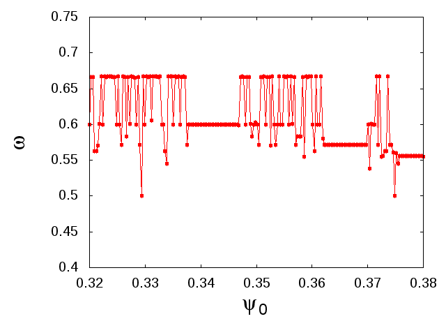
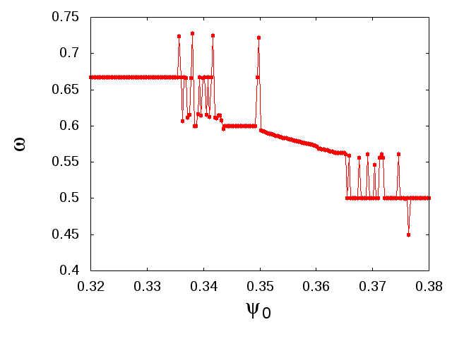
First we consider the dynamics determined by the Hamiltonian $H+v$ with $H$ and $v$ as in equations (2) and (3). We set $\varepsilon=0.0012$ and we compute the map relative to the interval $0.32<\psi_{0}<0.38$ , evenly distributed around $\Psi=0.35$ . Then we add the control term $f$ given by equation (10) and we repeat the analysis. The two FAMs are reported in figures and . In the case without control term the graphics is dominated by scattered points, which correspond to chaotic regions, and flat branches, corresponding to resonances. On the right (in presence of the control term), the graphics is also dominated mostly by resonances, but there is also a regularly decreasing region (where the behavior looks linear), approximately for $0.35\leq\psi_{0}\leq 0.365$ . According to the basics of the FAM method, this corresponds to a zone of the phase space that is filled with invariant (KAM) tori. We observe that, even though we localized the Hamiltonian around $\Psi=0.35$ to compute the control term, the invariant tori do not appear around $\Psi$ , but they are displaced to its right. This is usually seen also in KAM theory.

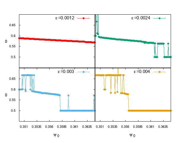
Next we computed different FAMs on the interval $0.35\leq\psi_{0}\leq 0.365$ , increasing the value of $\varepsilon$ . The results are reported in the four boxes of figure 3. As $\varepsilon$ is doubled from $0.0012$ to $0.0024$ , the width of the regular pattern is left nearly unchanged; then it slowly shrinks, as $\varepsilon$ increases, leaving space for more chaos and resonances. At $\varepsilon=0.003$ the width of the barrier is more than halved, while at $\varepsilon=0.004$ (the value considered in [7]) it is extremely small. Two similar plots (that we omit for the sake of brevity) allows us to fix to $\varepsilon^{*}\in(0.0045\,,\,0.0046)$ the threshold value for the disappearance of the invariant tori separating the chaotic regions. In particular, for $\varepsilon=0.0046$ the results provided by the FAM (in the case of the controlled Hamiltonian $H+v+f$ ) have the same look with respect to those reported in figure (corresponding to the uncontrolled case $H+v$ ).

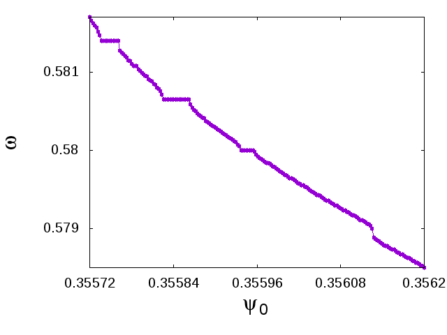
Finally, we perform a further magnification of the interval $0.35572\leq\psi_{0}\leq 0.3562$ in the case $\varepsilon=0.004$ ; this is reported in figure 4. At this value of the perturbation parameter we have a good compromise among being close to the breaking threshold of the invariant tori, and being able to distinguish the linear region of the FAM. In figure 4 there are four small plateau, corresponding to the (resonant) frequencies

\omega_{1}\,=\,\frac{25}{43}\,\approx\,0.5813968\,,\quad\omega_{2}\,=\,\frac{43}{74}\,\approx\,0.5810763\,,\quad\omega_{3}\,=\,\frac{18}{31}\,\approx\,0.5806491\,,\quad\omega_{4}\,=\,\frac{29}{50}\,\approx\,0.5799930

(11)

On the right we also see a vertical jump, denoting the presence of a hyperbolic point.

We are interested in the most robust tori (identified by their frequencies) of the controlled system. They should be the last to survive to the perturbation, and we want to target (one of) them with the CAP of the next section. By the method of the Farey tree [20] we can take two rational numbers and build a so called noble torus in between them, according to [24] it is expected to be the most robust in a local sense. The frequencies corresponding to the plateau are rational numbers (because they correspond to resonant orbits): so we pose that by the Farey tree, starting from the frequencies (11), we can find three robust tori of this dynamical system. Given two rational numers $n_{1}/d_{1}$ and $n_{2}/d_{2}$ , the “most noble” number in between is $(n_{1}+\sigma n_{2})/(d_{1}+\sigma d_{2})$ , being $\sigma=(\sqrt{5}+1)/2$ , the so-called golden mean.

By trial and error, we have seen that a robust frequency is

\omega_{D}\,=\,\frac{43+\sigma 18}{74+\sigma 31}\,\approx\,0.580905,

(12)

built by applying the Farey tree to the couple $\omega_{2},\,\omega_{3}$ .

3 CAP of the existence of a KAM torus

In this section we describe the scheme of a Computer Assisted Proof (based on KAM theory) to prove the existence of an invariant torus for a Hamiltonian system.

In the constext of classical mechanics, KAM theory denotes a set of methods to build invariant tori for perturbations of integrable Hamiltonian systems [14]. To be more precise, it is possible to show that a dense set of invariant tori of an integrable Hamiltonian are only deformed in presence of a (small) perturbation. Let us remark that the control theory of M. Vittot (that we used in section 1) is built in strong analogy with KAM theory, as discussed in [28].

The KAM algorithm we are going to use was introduced in [15] and [14]; it was used for a CAP in [6], and then also in [23] and [13]. It is based on classical series expansions for the Hamiltonian function, with no use of the so-called quadratic method. By applying this algorithm to a Hamiltonian of the type (5) for the model of the magnetic field, at the end of the $r$ -th step of the algorithm, we get

H^{(r)}\,=\,\omega\psi\,+\,P\,+\,\sum_{l=2}^{l_{\text{max}}}\sum_{s\geq 0}F_{l}^{(r,s)}\,+\,\sum_{s\geq r+1}\,\big(F_{0}^{(r,s)}\,+\,F_{1}^{(r,s)}\big)

(13)

with $F_{l}^{(r,s)}\in\mathbb{P}_{l,sK}$ , K can be defined as in section 1 as the trigonometric degree of the perturbation $v$ , or equivalently as the highest trigonometric degree of the terms $F_{0,1}^{(0,s)}$ . By an infinite number of transformations, the initial Hamiltonian $H^{(0)}$ can be transformed to its Kolmogorov Normal Form

H^{(\infty)}\,=\,\omega\psi\,+\,P\,+\,\sum_{l=2}^{l_{\text{max}}}\sum_{s\geq 0}F_{l}^{(\infty,s)}

(14)

that has a manifestly invariant torus $\psi=0$ on which the motion takes place with frequency $\omega$ .

In our CAP we begin by computing explicitly a finite number of KAM transformations, from $r=0$ to $r=R_{I}$ . Then, we iterate estimates on upper bounds for the coefficients of the transformed Hamiltonians, from $r=R_{I}+1$ up to $r=R_{I\!I}$ . In [6] it was discussed how a clever combination of the two techniques provides the best compromise between time-efficiency (the explicit computations are more demanding in terms of computing time) and numerical precision (in the iteration of the estimates we introduce a lot of approximations). Finally, we show that $H^{(R_{I\!I})}$ satisfies all the hypothesis of a KAM theorem, so it can be conjugated by an analytical canonical transformation to the Kolmogov Normal Form (14) of $H^{(0)}$ .

The present section just aims at giving a well defined procedure leading to a complete CAP, in such a way to perfectly fit with the present context. Therefore, in the following the justifications for both the formal algorithm and the scheme of the estimates will not be discussed at all. Their validity can be checked by referring to the already mentioned works dealing with CAPs that are designed in such a way to apply the KAM theorem.

In all of our codes that we wrote to perform the CAP we implemented validated numerics so as to ensure fully rigorous results. A detailed discussion of validated numerics was given in appendix A of [4]

The codes performing the CAP are freely available from the Mendeley Data repository. They are collected in a software package¹¹ 1 That software package can be freely downloaded from the web address http://dx.doi.org/10.17632/jdx22ysh2s.1, to which hereafter we will refer as the supplementary material that is related to this paper. In order to increase their readability, they are rather well commented and the structure of the whole software package should be easy to understand starting from the detailed explanations included in the file README.txt. We implemented the explicit KAM transformations in the program expl_trasf.c and the iteration of the estimates in the program iteration+proof.c; the latter also computes the parameters that appear in the statement of the KAM theorem. In the following, we will refer sometimes to the names of the functions that are written in C programming language and are included in the files making part of the supplementary material. These references will be done in order to eventually defer the reader to the algorithmic counterpart of our explanations, when this can be seen as convenient for a better understanding.

3.1 Description of the KAM algorithm

At the beginning of the $r$ -th step of the algorithm the Hamiltonian looks like

H^{(r-1)}\,=\,\omega\psi\,+\,P\,+\,\sum_{l=2}^{l_{\text{max}}}\,\sum_{s\geq 0}\,F_{l}^{(r-1,s)}\,+\,\sum_{s\geq r}\,\Big(F_{0}^{(r-1,s)}\,+\,F_{1}^{(r-1,s)}\Big)

(15)

where (again) $F_{l}^{(r-1,s)}\in\mathbb{P}_{l,sK}$ . In principle the Hamiltonian has an infinite number of coefficients, but in our code they are truncated to a maximum trigonometric degree²² 2 However, at each step we compute the norms of the terms whose trigonometric degree is bigger than $2KR_{I}$ . They are also exported and will be used as an input for the iteration of the estimates. of³³ 3 The factor $2$ stems from the number of angular variables that are considered in the system. $2KR_{I}$ . For the representation of the Taylor-Fourier coefficients we employed a technique based on the so-called “indexing functions” which is described in detail in [18]. From equation (15) (but also from equation (13)) it is evident that the main part of the angular average applied to the linear term of the Hamiltonian (i.e., $\omega\psi\,+\,P$ ) has a different role with respect to the other summands. Indeed, KAM algorithms are usually designed to preserve the frequency $\omega$ . In our code, this value is stored apart from the rest of the Hamiltonian, so it cannot be affected by numerical errors related to the performing of the Lie series⁴⁴ 4 Of course, it is still subject to the interval arithmetics. .

To the Hamiltonian (15) we apply three Lie series, according to the rule

e^{\{g\}}H\,=\,\sum_{j=0}^{\infty}\,\frac{1}{j!}\,{\{g\}^{j}}H

(16)

that is implemented in our code by calling the function $\mathtt{can\_transf\_ham}$ . The number of operations performed by this function is always finite because the functions are truncated so that the maximum trigonometric degree of the result does not exceed $2KR_{I}$ .

The first generating function $X^{(r)}\in\mathbb{P}_{0,rK}$ is given by

X^{(r)}\,=-\Gamma_{\omega}\,F_{0}^{(r-1,r)}.

(17)

As in section 1, the operator $\Gamma_{\omega}$ is well defined if the frequency $\omega$ is non-resonant⁵⁵ 5 This hypothesis is satisfied if $\omega$ is a Diophantine number, as we often assume in KAM theory. . Also, the operator $\Gamma_{\omega}$ is well defined on a zero-average function; the average of $F_{0}^{(r-1,r)}$ is a constant and can be safely ignored. The effect of the Lie transform generated by $\{X^{(r)}\}$ is exactly to erase $F_{0}^{(r-1,r)}$ .

The operator $\Gamma_{\omega}$ is implemented in our code by the function solve_homol_eq which moves the Fourier coefficients of $F_{0}^{(r-1,r)}$ from the Hamiltonian to the variable $\mathtt{target\_fn}$ , and use them to compute the coefficients of $X^{(r)}$ (stored in the variable $\mathtt{gen\_fn}$ ).

The second generating function is $\xi^{(r)}\theta$ , and the corresponding transform is a translation of the action $\psi$ by a quantity $\xi^{(r)}$ . The effect of this second transform is to erase $\langle F_{1}^{(r-1,r)}\rangle$ , where $\langle F_{l}^{(r,s)}\rangle$ is the average of a generic function $F_{l}^{(r,s)}$ with respect to the angle variables $\theta$ and $\varphi$ , for all $0\leq l\leq l_{\text{max}}$ and non-negative indexes $r,\,s$ . To fix the ideas, by referring to the decomposition described in equation (4), $\langle g\rangle$ is nothing but the coefficient $g_{l,0,0}$ corresponding to the harmonic $(k_{1}=0,k_{2}=0)$ appearing in the Taylor-Fourier expansion of $g\in\mathbb{P}_{l,s}\,$ . Let us define

C^{(r)}\,=\,\sum_{s=0}^{r}\partial_{\psi\psi}^{2}\langle F_{2}^{(r-1,s)}\rangle

(18)

and impose

C^{(r)}\,\xi^{(r)}\,+\,\langle F_{1}^{(r-1,r)}\rangle\,=\,0.

(19)

Equation (19) is solved in our code by the function $\mathtt{solve\_transl\_eq}$ . For a $1\tfrac{1}{2}$ d.o.f. system, $C$ is a scalar, but in general it is a matrix which needs to be inverted; this operation is performed by the function $\mathtt{calc\_inv\_matr\_C}$ , after removing the average of the quadratic term of the Hamiltonian through the function move_average_to. Finally we need a function readd_lie_series_csiq_average_terms to add back the average of the quadratic terms and the constant term that should have been produced by the action of the second Lie series on the average of the quadratric term, that instead we removed.

Sometimes the first two generating functions are grouped into⁶⁶ 6 This is expecially meaningful when the two trasforms are defined so as to commute; unfortunately, this is not our case, because to compute $\xi^{(r)}$ we also need the coefficient $F_{2}^{(r-1,r)}$ which is affected by the action of $X^{(r)}$ . Nevertheless we will use this type of notation because it is useful for the next section. $\chi_{1}^{(r)}\,=\,X^{(r)}+\xi^{(r)}\theta$ . Then, we introduce the intermediate Hamiltonian⁷⁷ 7 Note that, by the action of $e^{\{\chi_{1}^{(r)}\}}$ on a Hamiltonian with a finite expansion in all variables, we get another Hamiltonian with finite expansion. In fact, as $\{\chi_{1}^{(r)}\}g\,=\,\big(\partial_{\theta}X^{(r)}(\theta,\varphi)\,+\,\xi^{(r)}\big)\partial_{\psi}g$ when we act with $e^{\{\chi_{1}^{(r)}\}}$ on a Hamiltonian like (5), the Lie series can be applied $l_{\text{max}}$ times at most. In particular, if the trigonometric degree of the original Hamiltonian is $R_{h}K$ and that of the generating function is $R_{g}K$ , the transformed Hamiltonian has trigonometric degree $(R_{h}+l_{\text{max}}R_{g})K$ .

$\displaystyle\hat{H}^{(r)}$	$\displaystyle=\,e^{\{\chi_{1}^{(r)}\}}H^{(r-1)}$	(20)
	$\displaystyle=\,\omega\psi\,+\,P\,+\sum_{l=2}^{l_{\text{max}}}\,\sum_{s\geq 0}\hat{F_{l}}^{(r,s)}\,+\,\hat{F_{1}}^{(r,r)}\,+\,\sum_{s\geq r+1}\,\Big(\hat{F_{0}}^{(r,s)}+\,\hat{F_{1}}^{(r,s)}\Big)\,,$
$\displaystyle\hat{F_{1}}^{(r,r)}$	$\displaystyle=\,F_{1}^{(r-1,r)}\,-\,\langle F_{1}^{(r-1,r)}\rangle\,+\,\big(\partial_{\psi}\langle F_{2}^{(0)}\rangle\big)\big(\partial_{\theta}X^{(r)}\big).$

After an inspection of equation (20) we realize that we want to erase the term $\hat{F_{1}}^{(r,r)}$ . The latter is zero-average thanks to the translation by $\xi^{(r)}$ , so we can define the third generating function $\chi_{2}^{(r)}\in\mathbb{P}_{1,rK}$ by another homological equation,

\chi_{2}^{(r)}\,=\,-\Gamma_{\omega}\,\hat{F_{1}}^{(r,r)}.

(21)

The Lie series generated by $\chi_{2}^{(r)}$ maps $\hat{H}^{(r)}$ to the the Hamiltonian $H^{(r)}$ of equation (13). To solve this second homological equation we invoke again the function solve_homol_eq. In this second case, we still need the term $\hat{F_{1}}^{(r,r)}$ after its deletion. Indeed, we have

e^{\{\chi_{2}^{(r)}\}}\Big(\omega\psi\,+\,P\,+\,\hat{F_{1}}^{(r,r)}\Big)\,=\\ =\,\omega\psi\,+\,P\,+\{\chi_{2}^{(r)}\}(\omega\psi+P)\,+\,\hat{F_{1}}^{(r,r)}\,+\,\sum_{j\geq 1}\frac{1}{(j+1)!}\{\chi_{2}^{(r)}\}^{j}\Big(\{\chi_{2}^{(r)}\}(\omega\psi+P)\,+\,(j+1)\hat{F_{1}}^{(r,r)}\Big)\,=\\ =\,\omega\psi\,+\,P\,+\,\sum_{j\geq 1}\frac{j}{(j+1)!}\{\chi_{2}^{(r)}\}^{j}\hat{F_{1}}^{(r,r)}.

(22)

This means that we need $\hat{F_{1}}^{(r,r)}$ to transform the expansion of terms appearing in $\hat{H}^{(r)}$ to that corresponding to $H^{(r)}$ . This is why the function solve_homol_eq copied $\hat{F_{1}}^{(r,r)}$ to the variable $\mathtt{target\_fn}$ . The coefficients of the last term of equation (22) are computed by the function $\mathtt{readd\_lie\_series\_chi2\_target\_term}$ .

The terms appearing into the expansions of $\hat{H}^{(r)}$ and $H^{(r)}$ can be computed according to the formulae (28)-(31) of⁸⁸ 8 To translate to our notation it is sufficient to make the replacements $\displaystyle f_{l}^{(r,s)}\mapsto F_{l}^{(r,s)}\,,\quad l\geq 0\,,\,s\geq r+1$ (23) $\displaystyle h_{l}^{(s)}\mapsto F_{l}^{(r,s)}\,,\quad l\geq 2\,,\,0\leq s\leq r$ (24) and two analogous rules for hatted quantities. [23].

We recall here that all the computations are performed with interval arithmetics. The machine represents real numbers by floating point numbers, which however do not have the same properties of reals. As a consequence, to make numerical results rigorous, it is possible to replace a real number by two floating point numbers, representing the upper and lower bound of the original real number in its floating point representation. For this purpose, in our code we employed an aptly defined type called INTERVAL. Evidently, all the elementary operations have to be redefined for intervals; the principle to do so is explained in appendix A of [6] (short version) and also in appendix A of [4] (long version). In our code, the implementation of the operations for intervals is found in the file int_arit_lib.c.

3.2 Iteration of the Estimates

Given $g\in\mathbb{P}_{l,s}$ (see equation (4)) we introduce the norm

\|g\|\,=\,\sum_{\max(|k_{1}|,|k_{2}|)\leq s}|g_{l,k_{1},k_{2}}|.

(25)

So we introduce an upper bound for the norm of any function that we computed explicitly in the preceding section. First we define, for any $1\leq r\leq R_{I}$ , the four constants⁹⁹ 9 If the system was not degenerate in the variable $P$ , we would replace $\partial_{\theta}\mapsto\max\big(\partial_{\theta},\partial_{\varphi}\big)$ , $|\xi^{(r)}|\mapsto\max\big(|\xi_{1}^{(r)}|,|\xi_{2}^{(r)}|\big)$ , and finally $\partial_{\psi}\mapsto\max\big(\partial_{\psi}\,;\,\partial_{P}\big)$ .

\mathcal{G}_{1,1}^{(r)}\,=\,\big\|\partial_{\theta}X^{(r)}\big\|\,,\quad\mathcal{G}_{1,2}^{(r)}\,=\,|\xi^{(r)}|\,,\quad\mathcal{G}_{2,1}^{(r)}\,=\,\big\|\partial_{\theta}\chi_{2}^{(r)}\big\|\,,\quad\mathcal{G}_{2,2}^{(r)}\,=\,\big\|\partial_{\psi}\chi_{2}^{(r)}\big\|.

(26)

Second, we need sets of constants to bound from above the terms appearing in the expansions of the Hamiltonians $H^{(r)}$ and $\hat{H}^{(r)}$ ; for all $1\leq r\leq R_{I\!I}$ we call them $\mathcal{F}_{l}^{(r,s)}$ , $\hat{\mathcal{F}}_{l}^{(r,s)}$ , and $\mathcal{B}^{(r,s)}$ , and we define them so that, for all $1\leq r\leq R_{I}$ ,

		$\displaystyle\mathcal{F}_{l}^{(r,s)}\,=\,\\|F_{l}^{(r,s)}\\|\,,\quad\hat{\mathcal{F}}_{l}^{(r,s)}\,=\,\\|\hat{F_{l}}^{(r,s)}\\|\,,\qquad l=0,1,\,r\leq s\leq R_{I}\,,$		(27)
		$\displaystyle\mathcal{F}_{l}^{(r,s)}\,=\,\\|F_{l}^{(r,s)}\\|\,,\quad\hat{\mathcal{F}}_{l}^{(r,s)}\,=\,\\|\hat{F_{l}}^{(r,s)}\\|\,,\qquad 2\leq l\leq l_{\text{max}},\,0\leq s\leq R_{I}.$		(27)

The values of the right hand side of equation (26) and (27) are computed by the program expl_trasf.c and written on an output file bounds_expl_expans.bin, for all $1\leq r\leq R_{I}$ . The values written on this file are read in the program iteration+proof.c by the functions read_gen_fun_bounds and read_ham_bounds.

We have now to face the problem of providing upper bounds for all those terms that appear in the expansions of the Hamiltonians defined by the normalization algorithm and are of type $\mathbb{P}_{l,sK}$ with $0\leq l\leq l_{\text{max}}$ and $R_{I}<s\leq R_{I\!I}\,$ . Their representations in Taylor-Fourier series is still finite, but they include so many terms that such functions are hard to be explicitly calculated. Nevertheless, an efficient scheme of iterative estimates can be settled also for this kind of functions so to greatly improve the final accuracy of the results provided by the CAP, when $R_{I\!I}\gg R_{I}\gg 1$ , as it has been widely discussed in [6]. For such a purpose, we have to properly extend the definition of the multi-indicial finite sequencies $\mathcal{F}_{\cdot}^{(\cdot,\cdot)}$ and $\hat{\mathcal{F}}_{\cdot}^{(\cdot,\cdot)}$ so that the following inequalities hold true for all $1\leq r\leq R_{I\!I}\,$ :

		$\displaystyle\\|F_{l}^{(r,s)}\\|\,\leq\,\mathcal{F}_{l}^{(r,s)}\,,\quad\\|\hat{F_{l}}^{(r,s)}\\|\,\leq\,\hat{\mathcal{F}}_{l}^{(r,s)}\,,\qquad l=0,1\,,\,r\leq s\,,\,R_{I}<s\leq R_{I\!I}\,,$		(28)
		$\displaystyle\\|F_{l}^{(r,s)}\\|\,\leq\,\mathcal{F}_{l}^{(r,s)}\,,\quad\\|\hat{F_{l}}^{(r,s)}\\|\,\leq\,\hat{\mathcal{F}}_{l}^{(r,s)}\,,\qquad 2\leq l\leq l_{\text{max}}\,,\,0\leq s\leq R_{I\!I}.$		(28)

Moreover, it is also convenient to define another multi-indicial set of positive values $\mathcal{B}^{(\cdot,\cdot)}$ so that

\|<\hat{F_{1}}^{(r,s)}>\|\,\leq\,\mathcal{B}^{(r,s)}\,,\quad R_{I}\leq r\leq s\leq R_{I\!I}.

(29)

These three finite sequencies are fully defined according to the prescriptions given in the following two sections 3.2.1 and 3.2.2.

3.2.1 Bounds on the generating functions

To grant the solvability of the homological equation at each step, we assume that there exists, for each value of the step index $r$ , a positive constant $\alpha_{r}$ such that

\big|k_{1}\omega+k_{2}\big|\,\geq\,\alpha_{r}

(30)

and which can be simply computed by setting

\alpha_{r}\,=\,\min_{0<\max(|k_{1}|,|k_{2}|)\leq rK}\Big(\big|k_{1}\omega+k_{2}\big|\Big).

(31)

In both (30) and (31) $k_{1}$ and $k_{2}$ are integers numbers that cannot be simoultaneously zero. We recall that the constant $K$ was defined in section 1 as the trigonometric degree of the perturbation $v$ . Note that the existence of a positive constant $\alpha_{r}$ for $1\leq r\leq R_{I}$ is granted by the fact that the explicit computation can be performed. We need to compute its value only for $R_{I}<r\leq R_{I\!I}$ .

From equation (17), we find

\|X^{(r)}\|\,\leq\,\frac{1}{\alpha_{r}}\,\|F_{0}^{(r-1,r)}\|.

(32)

Therefore, by analogy with (26) we define, for all $R_{I}<r\leq R_{I\!I}$ ,

\mathcal{G}_{1,1}^{(r)}\,=\,\frac{rK}{\alpha_{r}}\mathcal{F}_{0}^{(r-1,r)}.

(33)

In a similar way, from equation (21) we can deduce

\|\chi_{2}^{(r)}\|\,\leq\,\frac{1}{\alpha_{r}}\|F_{1}^{(r-1,r)}\|\,\implies\,\mathcal{G}_{2,1}^{(r)}\,=\,\frac{rK\hat{\mathcal{F}}_{1}^{(r-1,r)}}{\alpha_{r}}\,,\quad\mathcal{G}_{2,2}^{(r)}\,=\,\frac{\hat{\mathcal{F}}_{1}^{(r-1,r)}}{\alpha_{r}}.

(34)

These equalities hold, again, for $R_{I}<r\leq R_{I\!I}$ .

Finally, let us assume that there exists a positive constant $m^{(r)}$ such that $m^{(r)}\leq|C^{(r)}|$ , then

|\xi^{(r)}|\,\leq\,(m^{(r)})^{-1}\,\|\langle F_{1}^{(r-1,r)}\rangle\|\implies\mathcal{G}_{1,2}^{(r)}\,=\,(m^{(r)})^{-1}\,\mathcal{B}^{(r,r)}.

(35)

The direct computation of $m^{(R_{I})}$ is obvious in our $1\tfrac{1}{2}$ d.o.f. example, and it could be also computed in dimension $n>1$ as the eigenvalue of the Hessian of $H^{(R_{I})}$ with the lowest modulus. Moreover, it is easy to show that this constant can be updated recursively according to the following rule

m^{(r)}\,=\,m^{(r-1)}\,-\,2\,\mathcal{F}_{2}^{(r-1,r)}\,,\quad\forall\,R_{I}<r\leq R_{I\!I}.

(36)

3.2.2 Bounds on the transformed Hamiltonian

Given the bounds on the generating functions, we can deduce those on the terms appearing in the expansion of a transformed Hamiltonian $H^{(r)}$ starting from that corresponding to $H^{(r-1)}$ for all $1\leq r\leq R_{I\!I}\,$ . In the case of the transformation generated by $\chi_{1}^{(r)}$ ,

\Big\|\frac{1}{j!}\,\{\chi_{1}^{(r)}\}^{j}g\Big\|\,\leq\,\binom{l}{j}\Big(\big\|\partial_{\theta}X^{(r)}\big\|\,+\,\big|\xi^{(r)}\big|\Big)^{j}\,\|g\|.

(37)

If we assume that $g\in\mathbb{P}_{l,sK}$ , then $\{\chi_{1}^{(r)}\}^{j}g\in\mathbb{P}_{l-j,(s+rj)K}$ . So we can update the upper bounds on the terms appearing in the expansion of the Hamiltonian $H^{(r-1)}$ (that appear in formula (15) and are assumed to be initialized when $r-1=0$ ) according to the following rules¹⁰¹⁰ 10 We introduce the symbol $\,\mathtt{+\!=}\,$ (familiar to the C programmers) so that $a\,\mathtt{+\!=}\,b$ is equivalent to a redefinition of the value of $a$ in such a way that $a\mapsto a+b$ . : $\hat{\mathcal{F}}_{l}^{(r,s)}=\mathcal{F}_{l}^{(r-1,s)}$ $\forall\,l,\,s$ , $\hat{\mathcal{F}}_{0}^{(r,r)}=0$ and

\begin{gathered}\hat{\mathcal{F}}_{l-j}^{(r,s+jr)}\,\,\mathtt{+\!=}\,\,\binom{l}{j}\Big(\mathcal{G}_{1,1}^{(r)}\,+\,\mathcal{G}_{1,2}^{(r)}\Big)^{j}\mathcal{F}_{l}^{(s,s)}\,,\qquad\forall\,l\geq 2,\,0\leq s<r,\,1\leq j\leq l,\,R_{I}<s+jr\leq R_{I\!I}\,,\\ \hat{\mathcal{F}}_{l-j}^{(r,s+jr)}\,\,\mathtt{+\!=}\,\,\binom{l}{j}\Big(\mathcal{G}_{1,1}^{(r)}\,+\,\mathcal{G}_{1,2}^{(r)}\Big)^{j}\mathcal{F}_{l}^{(r-1,s)}\,,\qquad\forall\,l\geq 1,\,s\geq r,\,1\leq j\leq l,\,R_{I}<s+jr\leq R_{I\!I}.\\ \end{gathered}

(38)

In the case of the trasformation generated by $\chi_{2}^{(r)}$ , the following inequality holds true for any $g\in\mathbb{P}_{l,sK}\,$ :

\Big\|\frac{1}{j!}\,\{\chi_{2}^{(r)}\}^{j}g\Big\|\,\leq\,\frac{1}{j!}\,\prod_{i=0}^{j-1}\Big[l\big\|\partial_{\theta}\chi_{2}^{(r)}\big\|\,+\,\big((s+ir)K\big)\big\|\partial_{\psi}\chi_{2}^{(r)}\big\|\Big]\,\|g\|.

(39)

Since $\{\chi_{2}^{(r)}\}^{j}g\in\mathbb{P}_{l,(s+rj)K}$ , a second set of rules easily follows: $\mathcal{F}_{l}^{(r,s)}=\hat{\mathcal{F}}_{l}^{(r,s)}$ $\forall\,l,\,s$ , $\mathcal{F}_{1}^{(r,r)}=0$ and

\begin{gathered}\mathcal{F}_{l}^{(r,s+jr)}\,\,\mathtt{+\!=}\,\,\frac{1}{j!}\,\prod_{i=0}^{j-1}\Big[l\mathcal{G}_{2,1}^{(r)}\,+\,\big((s+ir)K\big)\mathcal{G}_{2,2}^{(r)}\Big]\hat{\mathcal{F}}_{l}^{(s,s)}\,,\qquad\forall\,l\geq 2,\,0\leq s\leq r,\,j\geq 1,\,R_{I}<s+jr\leq R_{I\!I}\,,\\ \mathcal{F}_{l}^{(r,s+jr)}\,\,\mathtt{+\!=}\,\,\frac{1}{j!}\,\prod_{i=1}^{j}\Big[l\mathcal{G}_{2,1}^{(r)}\,+\,\big((s+ir)K\big)\mathcal{G}_{2,2}^{(r)}\Big]\hat{\mathcal{F}}_{l}^{(s,s)}\,,\qquad\forall\,l\geq 0,\,s>r,\,j\geq 1,\,\,R_{I}<s+jr\leq R_{I\!I}\,,\\ \mathcal{F}_{1}^{(r,(j+1)r)}\,\,\mathtt{+\!=}\,\,\frac{1}{j!}\,\prod_{i=1}^{j}\Big[\mathcal{G}_{2,1}^{(r)}\,+\,\big((i+1)rK\big)\mathcal{G}_{2,2}^{(r)}\Big]\hat{\mathcal{F}}_{1}^{(r,r)}\,,\qquad\forall\,j\geq 1,\,R_{I}<(j+1)r\leq R_{I\!I}.\end{gathered}

(40)

For what concerns the angular average of the perturbing terms that are linear in $\psi$ , we need to refine the iterative definitions with respect to those provided for $\mathcal{F}_{1}^{(r,s)}$ . This can be made by using sharper evaluations preventing a deterioration effect that would be due to the fact that the majorant $\mathcal{G}_{1,2}^{(r)}$ would contribute to the definition of $\mathcal{G}_{1,2}^{(s)}$ for any $s=r+1,\,\ldots\,2r-1$ . Indeed, a so strict recursion is artificious and can be avoided by slightly adapting the scheme of estimates in the following suitable way. After having recalled the equations (17)–(22), for every $r\geq R_{I}+1$ it is convenient to set

\begin{gathered}\mathcal{B}^{(r,s)}=\mathcal{F}_{1}^{(r,s)}\,,\qquad{\rm if}\ r=R_{I}+1\ \forall\,r\leq s\leq R_{I\!I}\,,\ {\rm else}\ \forall\,2r-2\leq s\leq R_{I\!I}\,,\\ \mathcal{B}^{(r,s+r)}\,=\,\mathcal{B}^{(r-1,s+r)}+2\mathcal{G}_{1,1}^{(r)}\mathcal{F}_{2}^{(r-1,s)}\,,\qquad\forall\,1\leq s<r,\,\,R_{I}<s+r\leq R_{I\!I}.\\ \end{gathered}

(41)

Formulae appearing in (38) and (40) are implemented in our program iteration+proof.c by the functions $\mathtt{calc\_estimates\_ham\_chi1}$ and $\mathtt{calc\_estimates\_ham\_chi2}$ , respectively. Both are invoked for all $1\leq r\leq R_{I\!I}$ . Here, let us recall that the constants $\mathcal{F}_{l}^{(r,s)}$ need not to be computed by the recursive relations for $r,s\leq R_{I}$ , because they are evaluated as norms of functions, whose expansions are explicitly computed according to the prescriptions described in subsection 3.1. Formulae appearing in (41) are implemented by the function $\mathtt{calc\_estimates\_ave\_ham\_chi1}$ that is invoked for all $R_{I}+1\leq r\leq R_{I\!I}\,$ .

3.2.3 The recursive relations defining the parameters $\mathcal{E}_{r}$ , $\zeta_{r}$ and $a_{r}$

Of course, the expansions of the Hamiltonians contain an infinite number of terms. Therefore, we need upper bounds also for the norms of the functions $F_{l}^{(r,s)}$ with $s>R_{I\!I}$ . We stress that this kind of terms is neither explicitly calculated according the algorithm described in subsection 3.1 nor estimated as it has been explained in the previous subsection 3.2.2. Therefore, we need to introduce three sequencies $(\mathcal{E}_{r},\zeta_{r},a_{r})_{1\leq r\leq R_{I\!I}}$ , defined so that¹¹¹¹ 11 see for instance [14], [6], and [23]. at any step $r=1\,,\,\ldots\,,\,R_{I\!I}$ of the KAM algorithm the following inequalities are satisfied:

\|F_{l}^{(r,s)}\|\,\leq\,\mathcal{E}_{r}\,\zeta_{r}^{l}\,a_{r}^{s}\,,\quad\forall\,s>R_{I\!I}\,,\,0\leq l\leq l_{\text{max}}.\\

(42)

It is possible to derive recursive rules to compute these sequencies from the algorithm of section 3.1 (see for instance [14], [6]). These rules, which are not unique, involve also the norms of the generating functions. For $1\leq r\leq R_{I}$ , these norms were computed explicitly. Therefore, the bounds that we determine by the recursive definition of $(\mathcal{E}_{r},\zeta_{r},a_{r})_{r=R_{I}+1}^{R_{I\!I}}$ . are likely to be less sharp than those that we find when the explicit computations of the generating functions are involved.

In the KAM algorithm of section 3.1, during the $r$ -th normalization step we transform $H^{(r-1)}$ into an intermediate Hamiltonian $\hat{H}^{(r-1)}$ by the action of the Lie series operator $e^{\{\chi_{1}^{(r)}\}}$ , then we transform $\hat{H}^{(r-1)}$ into $H^{(r)}$ by the action of $e^{\{\chi_{2}^{(r)}\}}$ . Accordingly, we choose to update twice also the recursive inequalities, at each step, in the following way. Given $\mathcal{E}_{r-1}$ , $\zeta_{r-1}$ and $a_{r-1}$ , we compute

\begin{gathered}\hat{\mathcal{E}}_{r}\,=\,\mathcal{E}_{r-1}\bigg(1+\frac{\big(\,\mathcal{G}_{1,1}^{(r)}+\mathcal{G}_{1,2}^{(r)}\,\big)\zeta_{r-1}}{a_{r-1}^{r}}\bigg)^{l_{\text{max}}}\,,\quad\hat{\zeta}_{r}\,=\,\zeta_{r-1}\,,\quad\hat{a}_{r}\,=\,a_{r-1}\,,\qquad{\rm when}\ r\leq R_{I}\,,\\ \hat{\mathcal{E}}_{r}\,=\,\mathcal{E}_{r-1}\,,\quad\hat{\zeta}_{r}\,=\,\zeta_{r-1}\,,\quad\hat{a}_{r}\,=\,a_{r-1}\bigg(1+l_{\text{max}}\,\frac{\big(\,\mathcal{G}_{1,1}^{(r)}+\mathcal{G}_{1,2}^{(r)}\,\big)\zeta_{r-1}}{a_{r-1}^{r}}\bigg)^{\frac{1}{r}}\,,\qquad{\rm if}\ R_{I}<r\leq R_{I\!I}\,.\end{gathered}

(43)

and then

\begin{gathered}\mathcal{E}_{r}\,=\,\hat{\mathcal{E}}_{r}\,,\\ \zeta_{r}\,=\,\hat{\zeta}_{r}\bigg(1+\frac{\max\big(\,rK\mathcal{G}_{2,2}^{(r)}\,,\,\mathcal{G}_{2,1}^{(r)}\,\big)}{{\hat{a}}_{r}^{r}}\bigg)\,,\quad a_{r}\,=\,\hat{a}_{r}\bigg(1+\frac{\max\big(\,rK\mathcal{G}_{2,2}^{(r)}\,,\,\mathcal{G}_{2,1}^{(r)}\,\big)}{{\hat{a}}_{r}^{r}}\bigg)^{\tfrac{1}{r}}\,,\qquad{\rm when}\ r\leq R_{I}\,,\\ \zeta_{r}\,=\,\hat{\zeta}_{r}\,,\quad a_{r}\,=\,\hat{a}_{r}\bigg(1+\frac{(l_{\text{max}}+1)\max\big(\,rK\mathcal{G}_{2,2}^{(r)}\,,\,\mathcal{G}_{2,1}^{(r)}\,\big)}{\hat{a}_{r}^{r}}\bigg)^{\tfrac{1}{r}}\,,\qquad{\rm if}\ R_{I}<r\leq R_{I\!I}\,.\end{gathered}

(44)

Let us remark that we could keep $\zeta_{r}$ constant at the price of introducing a factor $l_{\text{max}}$ in the rule for $a_{r}$ , but this choice is advantageous (because the contribution of such a factor is made negligible) only when the exponent $1/r$ is small.

The program iteration+proof.c also invokes orderly the functions $\mathtt{update\_estimates\_param\_chi1}$ and $\mathtt{update\_estimates\_param\_chi2}$ to compute, respectively, the values of $\hat{\mathcal{E}}_{r},\,\hat{\zeta}_{r},\,\hat{a}_{r}$ and of $\mathcal{E}_{r},\,\zeta_{r},\,a_{r}\,$ , for all $1\leq r\leq R_{I\!I}\,$ .

To define the initial values $a_{1}$ , $\zeta_{1}$ and $\mathcal{E}_{1}$ we exploit the fact that the original Hamiltonian has a finite degree in both actions and angles; let us recall that they are equal to ${l_{\text{max}}}$ and $R_{I}K$ , respectively. The sequence $\{a_{r}\}_{r}$ is the most threatening one to achieve convergence of the CAP; it is non-decreasing and we want to initialize it to the smallest value compatible with the inequalities in formula (42), when $r=1$ . Therefore, we set

a_{1}\,=\,\max\big(\,K\mathcal{G}_{2,2}^{(1)}\,,\,\mathcal{G}_{2,1}^{(1)}\,\big)\,,\qquad\zeta_{1}\,=\,1\,,\qquad\mathcal{E}_{1}\,=\,\max_{\{0\leq l\leq l_{\text{max}}\,,\,0\leq s\leq R_{I}+l_{\text{max}}\}}\bigg(\frac{\hat{\mathcal{F}}_{l}^{(1,s)}}{a_{1}^{s}\zeta_{1}^{l}}\bigg).

(45)

These values are computed by the function initialize_estimates_param.

3.3 Statement of a KAM theorem

The formulation of KAM theorem we are going to consider is the one reported in [27], that is adapted to a slightly larger class of dynamical models. Indeed, it applies to systems including also a particular type of dissipation that is proportional to a constant factor $\eta$ , but also the conservative case with $\eta=0$ is covered. Moreover, the framework of the proof of that version of the KAM theorem is different with respect to what is assumed here, therefore, a little of effort for the adaptation to the present context is mandatory. For instance, in [27] the weighted Fourier norms are considered. In order to properly introduce them, let us first define the following complex sets: $\mathbb{D}_{(\rho,\sigma)}\,=\,\mathbb{G}_{\rho}\times\mathbb{T}_{\sigma}^{2}\,$ , where

\mathbb{G}_{\rho}\,=\,\big\{z\in\mathbb{C}\,\colon\,|z|<\rho\big\}\ ,\qquad\mathbb{T}_{\sigma}^{2}\,=\,\big\{\,(\tilde{\theta},\tilde{\varphi})\in\mathbb{C}^{2}\,\colon\,\big(Re(\tilde{\theta}),Re(\tilde{\varphi})\big)\in\mathbb{T}^{2},\,|Im(\tilde{\theta})|\leq\rho,\,|Im(\tilde{\varphi})|\leq\rho\,\big\}\ ,

(46)

being $\rho$ and $\sigma$ two positive real parameters. On the set $\mathbb{D}_{(\rho,\sigma)}$ we can define the functional norms

\|g\|_{(\rho,\sigma)}\,=\,\sum_{(k_{1},k_{2})\in\mathbb{Z}_{2}/(0,0)}\sup_{\psi\in\mathbb{G}_{\rho}}|g_{l,k_{1},k_{2}}|e^{(|k_{1}|+|k_{2}|)\sigma}.

(47)

In order to concile our notations with those of [27] let us now introduce

F_{0,1}^{(R_{I\!I})}\,=\,\sum_{s\geq R_{I\!I}+1}F_{0,1}^{(R_{I\!I},s)}\,,\quad F_{l}^{(R_{I\!I})}\,=\,\sum_{s\geq 0}F_{l}^{(R_{I\!I},s)}\,,2\leq l\leq l_{\text{max}}\,.

(48)

Theorem 3.1 of [27] can now be stated in the following way to fit with the context of the present approach.

Theorem 1.

Consider a Hamiltonian $H^{(R_{I\!I})}=\omega\psi+P+\sum_{l\geq 0}F_{l}^{(R_{I\!I})}$ , that is analytic on the domain $\mathbb{D}_{(\rho,\sigma)}=\mathbb{G}_{\rho}\times\mathbb{T}_{\sigma}^{2}$ defined in formula (46). Let us assume that

•

there exist positive numbers $\rho,\sigma,\lambda,E$ such that

\big\|F_{0}^{(R_{I\!I})}\big\|_{(\rho,\sigma)}\,\leq\,\lambda E\,;\quad\big\|F_{1}^{(R_{I\!I})}\big\|_{(\rho,\sigma)}\,\leq\,\frac{\lambda E}{2}\,;\quad\big\|F_{l}^{(R_{I\!I})}\big\|_{(\rho,\sigma)}\,\leq\,\frac{E}{2^{l}}\,,\ \forall\,l\geq 0\ ;

(49)

•

there are two positive constants $\gamma$ and $\tau\geq 1$ such that¹²¹² 12 This is usually known as the Diophantine condition. $|k_{1}\omega+k_{2}|\geq\gamma/(|k_{1}|+|k_{2}|)^{\tau}$ $\forall\,(k_{1}\,,\,k_{2})\neq(0,0)$ ;
•

there exists a positive constant $m$ such that $\big|\partial_{\psi\psi}^{2}\langle F_{2}^{(R_{I\!I})}\rangle\big|\,\geq\,m$ ;

•

the parameter $\lambda$ is so small that

\lambda<\lambda^{*}\,=\,\min\bigg(\frac{1}{20^{25+9\tau}\,\bar{W}^{2}\,\bar{Z}^{2}}\,;\,9\Big(\frac{m\rho^{2}}{Ee^{\pi^{2}/3}}\Big)^{2}\bigg)

(50)

where

	$\displaystyle\bar{A}\,=\,\frac{Ee^{\pi^{2}/3}}{\gamma}\Big(\frac{\tau}{e\sigma}\Big)^{\tau}\,,\qquad\bar{B}\,=\,\Big(1+\frac{\bar{A}}{e\rho\sigma}\Big)\frac{Ee^{\pi^{2}/3}}{m\rho}\ ,$		(51)
	$\displaystyle\bar{W}\,=\,\max\bigg(\frac{e^{2}}{\rho}\Big(\frac{\bar{A}}{e\sigma}\,+\,\bar{B}\Big)\,,\,2\bigg)\,,\qquad\bar{Z}\,=\,\max\bigg(\frac{2e\bar{A}}{\rho\sigma}\,,\,2\bigg)\ .$		(52)

Therefore, there exists a canonical analytical change of variables ${\cal C}\colon\mathbb{D}_{\tfrac{1}{2}(\rho,\sigma)}\to\mathbb{D}_{\tfrac{3}{4}(\rho,\sigma)}$ , transforming $H^{(R_{I\!I})}$ in the Kolmogorov Normal Form of type (14).

In order to apply the statement above, we need to choose four values of the parameters $\sigma$ , $\rho$ , $E$ and $\lambda$ so that the inequalities in (49) are satisfied. For this purpose, we have to reconsider the upper bounds that we introduced in the previous section 3.2. Let us remark that

\big\|F_{l}^{(R_{I\!I},s)}\big\|_{(\rho,\sigma)}\,\leq\big\|F_{l}^{(R_{I\!I},s)}\big\|\,\rho^{l}\,(e^{2K\sigma})^{s}

(53)

(where the form of the last multiplying coefficient is due to the fact that when the norm of $F_{l}^{(R_{I\!I},s)}$ is evaluated according to (47) we have that $|k_{1}|+|k_{2}|\leq 2sK$ , being the number of degrees of freedom equal to $2$ ) and so

	$\displaystyle\big\\|F_{0}^{(R_{I\!I})}\big\\|_{(\rho,\sigma)}\,\leq\,\mathcal{E}_{R_{I\!I}}\sum_{s\geq R_{I\!I}+1}(a_{R_{I\!I}}e^{2K\sigma})^{s}\,=\,\mathcal{E}_{R_{I\!I}}\frac{(a_{R_{I\!I}}e^{2K\sigma})^{(R_{I\!I}+1)}}{1-a_{R_{I\!I}}e^{2K\sigma}}\,,$		(54)
	$\displaystyle\big\\|F_{1}^{(R_{I\!I})}\big\\|_{(\rho,\sigma)}\,\leq\,\mathcal{E}_{R_{I\!I}}\sum_{s\geq R_{I\!I}+1}\,(\rho\zeta_{R_{I\!I}})\,(a_{R_{I\!I}}e^{2K\sigma})^{s}\,=\,\mathcal{E}_{R_{I\!I}}\,(\rho\zeta_{R_{I\!I}})\,\frac{(a_{R_{I\!I}}e^{2K\sigma})^{(R_{I\!I}+1)}}{1-a_{R_{I\!I}}e^{2K\sigma}}\,,$		(55)
	$\displaystyle\big\\|F_{l}^{(R_{I\!I})}\big\\|_{(\rho,\sigma)}\,\leq\,\sum_{s=0}^{R_{I\!I}}\,\mathcal{F}_{l}^{(R_{I\!I},s)}\rho^{l}(e^{2K\sigma})^{s}\,+\,\sum_{s\geq R_{I\!I}+1}\,\mathcal{E}_{R_{I\!I}}\,(\rho\zeta_{R_{I\!I}})^{l}\,(a_{R_{I\!I}}e^{2K\sigma})^{s}\,,\quad 2\leq l\leq l_{\text{max}}\,.$		(56)

By comparison of the formulae (54)–(56) and (49), it looks quite natural to set $\rho\,=\,(2\zeta_{R_{I\!I}})^{-1}$ . Moreover, the summation of the geometric series

\sum_{s\geq R_{I\!I}+1}(a_{R_{I\!I}}e^{2K\sigma})^{s}\,=\,\frac{(a_{R_{I\!I}}e^{2K\sigma})^{R_{I\!I}+1}}{1-a_{R_{I\!I}}e^{2K\sigma}}

(57)

is well defined provided that

\sigma\,<\,-\frac{1}{2K}\,\log(a_{R_{I\!I}})\,.

(58)

In order to define more conveniently the relation among $\sigma$ and the other parameters, we try to minimize the value of $\lambda/\lambda^{*}$ with respect to $\sigma$ ; with minor approximations we end up with $\sigma=4/(KR_{I\!I})$ . Finally, on the r.h.s. of equation (56) we can group a factor $(\rho\zeta_{R_{I\!I}})^{l}=2^{-l}$ , and we are naturally lead to define

E\,=\,\max_{2\leq l\leq l_{\text{max}}}\left(\zeta_{R_{I\!I}}^{-l}\,\sum_{s=0}^{R_{I\!I}}\mathcal{F}_{l}^{(R_{I\!I},s)}(e^{2K\sigma})^{s}\,+\,\mathcal{E}_{R_{I\!I}}\,\frac{(a_{R_{I\!I}}e^{2K\sigma})^{(R_{I\!I}+1)}}{1-a_{R_{I\!I}}e^{2K\sigma}}\right)

(59)

and

\lambda\,=\,\frac{\mathcal{E}_{R_{I\!I}}}{E}\,\frac{(a_{R_{I\!I}}e^{2K\sigma})^{R_{I\!I}+1}}{1-a_{R_{I\!I}}e^{2K\sigma}}\,.

(60)

The parameter $\gamma$ (that is entering the Diophantine inequality reported in the statement of theorem 1) is also computed in the program iteration+proof.c, by the function calc_gamma. The parameter $m$ that is also appearing in the hypothesis of theorem 1, can be identified with $m^{(R_{I\!I})}$ computed according to equation (36). The value of $m^{(R_{I})}$ is computed by the program expl_transf.c with the name coef_nondeg_matr_C, and written to the output file bounds_expl_expans; then it is read by the program iteration+proof.c and stored in the variable m_nondeg and updated for all $R_{I}+1\leq r\leq R_{I\!I}$ . Moreover, the values of the four parameters $\sigma$ , $\rho$ , $E$ and $\lambda$ are all computed by the function calc_param_proof in the program iteration+proof.c.

Therefore, at the end of its execution, the program iteration+proof.c can check if theorem 1 applies to the Hamiltonian $H^{(R_{I\!I})}$ . This is done by simply comparing the small parameter $\lambda$ with its threshold value $\lambda^{*}$ that is computed by using the definitions appearing in formulae (50)–(52).

4 Application to the problem of the controlled magnetic field

Here we want to apply the CAP (described in the previous section 3) to the problem of the controlled magnetic field (described in section 1). The controlled Hamiltonian is $\tilde{H}+f$ , see equations (5), and (8).

In the qualitative analysis of section 2 we have shown that we expect there is an invariant torus having frequency $\omega=\omega_{D}$ (see equation (12)), which is not the frequency corresponding to the torus that is labelled by $\psi=0$ and is invariant with respect to the flow of an integrable approximation of $\tilde{H}+f$ . It is convenient that such a property will be satisfied by $H^{(0)}$ , i.e., the initial Hamiltonian that is provided as an input for the whole CAP, which is based on the KAM algorithm (see section 3.1). The second type of Lie series, that we apply at each step of the KAM algorithm, performs a translation of the action and so it yields also a change of the frequency for the torus corresponding to $\psi=0$ in the approximation provided by the Kolmogorov normal form. Therefore, we decided to define $H^{(0)}$ by applying to $\tilde{H}+f$ a normalization step of the KAM algorithm as follows

H_{c}\,=\,e^{\{\chi_{2}\}}e^{\{\xi_{\text{init}}\theta\}}e^{\{X\}}\big(\tilde{H}+f\big)\,.

(61)

The value of $\xi_{\text{init}}$ is defined to bring the frequency we can associate to the torus corresponding to $\psi=0$ for the integrable approximation of $H_{c}$ as close as possible to $\omega_{D}$ , as we explain in the next subsection 4.1. Moreover, the generating function $X$ is determined according to formula (7), while also $\chi_{2}$ is given by an equation that is similar to that reported in (7), but it is aiming to remove the terms that are linear in $\psi$ and with Fourier harmonics $(k_{1}\,,\,k_{2})$ such that $0<\max(|k_{1}|,|k_{2}|)\leq K$ .

We can now introduce

H^{(0)}\,=\,\omega_{D}\psi\,+\,P\,+\,\sum_{l=0}^{l_{\text{max}}}\sum_{s=0}^{R_{I}}F_{l}^{(0,s)}

(62)

where $F_{l}^{(0,s)}\in\mathbb{P}_{l,sK}$ . $H^{(0)}$ is meant to be a truncation of the controlled Hamiltonian $H_{c}$ in the following sense. Let us write the Taylor-Fourier expansion for both of them

H_{c}=\sum_{l=0}^{l_{\text{max}}}\,\sum_{(k_{1}\,,\,k_{2})\in\mathbb{Z}^{2}}\,c_{l,k_{1},k_{2}}\,\psi^{l}\,e^{ik_{1}\theta+ik_{2}\varphi}\ ,\qquad H^{(0)}=\sum_{l=0}^{l_{\text{max}}}\,\sum_{(k_{1}\,,\,k_{2})\in\mathbb{Z}^{2}}\,d_{l,k_{1},k_{2}}\,\psi^{l}\,e^{ik_{1}\theta+ik_{2}\varphi}\ .

(63)

Then

d_{l,k_{1},k_{2}}=\left\{\vbox{\halign{ $\hfil\displaystyle{#}\hfil$\quad&$\displaystyle{#}\hfil$\cr c_{l,k_{1},k_{2}}&{\rm if}\ \max(|k_{1}|,|k_{2}|)\leq R_{I}K\cr 0&{\rm otherwise}\cr}}\right.

(64)

so that we have truncated the Fourier coefficients in such a way that the maximum trigonometric degree of the terms appearing in $H^{(0)}$ is not larger than $2KR_{I}$ (see section 3.1) before its expansion is passed to the program expl_transf.c. In figure 5 we plot the magnitude of the norms of the terms $F_{l}^{(0,s)}$ as a function of $s$ : we see that the truncation of the Fourier harmonics at $2KR_{I}$ is not a big issue when $R_{I}$ is large enough. In fact, for $s>90$ the magnitude of $\|F_{l}^{(0,s)}\|$ is even smaller than $10^{-45}$ $\forall\,l=0\,,\,\ldots\,,\,l_{\text{max}}\,$ .

The initial Hamiltonian $H^{(0)}$ is preliminarly calculated by using X $\rho$ ó $\nu o\varsigma$ , that is a software package especially designed for doing computer algebra manipulations into the framework of Hamiltonian perturbation theory (see [18] for an introduction to its main concepts). Such a code allows to represent the complete (and finite) expansion in Taylor-Fourier series of $H^{(0)}$ , in such a way to store it in the input (ASCII) file initial_Ham0.inp, that is read by the function def_init_ham, which makes part of the program expl_transf.c. A couple of intervals including the components of the angular velocity vector $\big(\omega_{D}\,,\,1\big)$ are written in another input file, namely freq_intervals.inp. Also for the sake of the usability of the codes making part of the supplementary material, we think it is preferable to not include there any software package that is depending on X $\rho$ ó $\nu o\varsigma$ . Therefore, in that material we have been forced to include the input files, that are initial_Ham0.inp and freq_intervals.inp. More precisely, they are stored in a subfolder, while in the main folder there are two different versions of those input files, that refer to an example of a slightly perturbed forced pendulum model, which is studied in [6]. This has been made for the sake of the (re)usability of the package provided in the supplementary material. Since the Taylor-Fourier representation of that Hamiltonian system is extremely shorter with respect to $H^{(0)}$ , which is defined as discussed above, our choice should allow to easily understand how the input files must be structured and modified in order to design further different applications.

Our main result is summarized by the following statement.

Theorem 2.

[Computer-Assisted] Consider the value $\varepsilon=0.003$ and the corresponding Hamiltonian $H^{(0)}$ that has been introduced by the procedure described in the present section, starting from the Hamiltonian $\tilde{H}+f$ which is fully defined by the equations (2)–(3), (5) and (10). Then, there exists a torus which is both invariant with respect to the Hamiltonian flow induced by $H^{(0)}$ and travelled by quasi-periodic motions characterized by the angular velocity vector $\big(\omega_{D}\,,\,1\big)$ .

In order to perform the CAP of the previous statement, it has been necessary to execute the algorithm discussed in the previous section 3.3 with $R_{I}=150$ and $R_{I\!I}=8500$ . This required a total computational time of about 62 hours on a workstation equipped with 2 CPU Intel XEON-GOLD 5220 (2.2 GHz) and 384 GB of RAM. Most of the time has been necessary for the explicit computation of the (truncated) expansions of the Hamiltonians $H^{(r)}$ for $r=1\,,\,\ldots\,,\,R_{I}=150$ ; this task has been made by running the program expl_transf.c.

In order to fix the ideas, let us report here the parameters entering in the estimates of the Hamiltonian $H^{(R_{I\!I})}$ that has been produced after the execution of $R_{I\!I}=8500$ normalization steps. Their values are

$\displaystyle{\rho\,=\,0.024215\,,}$	$\displaystyle{\sigma\,=\,0.00015686\,,}$	$\displaystyle{\lambda\,=\,10^{-91.5}\,,}$
$\displaystyle{E\,=\,0.0061441\,,}$	$\displaystyle{\gamma\,=\,0.24999\,,}$	$\displaystyle{m\,=\,1.3809\ .}$

(65)

The definitions appearing in formulae (50)–(52) allows to straightforwardly compute the threshold value of $\lambda^{*}=10^{-85.7}$ . Since the perturbation is so small that also the crucial hypothesis of theorem 1 is satisfied, i.e., $\lambda<\lambda^{*}$ , then the program iteration+proof.c claims that the wanted (invariant) torus exists in the final part of the output that is produced at the end of its execution.

4.1 Determination of $\xi_{\text{init}}$

Let us consider the Hamiltonian $H_{c}$ that is defined in equation (61). In particular, we focus on a single coefficient, i.e., $B(\xi_{\text{init}})=\langle\frac{\partial H_{c}}{\partial\psi}\rangle\big|_{\psi=0}\,$ . We aim to determine the value of the initial shift on the action $\psi$ , i.e., $\xi_{\text{init}}\in\mathbb{R}$ so that $B(\xi_{\text{init}})$ is as near as possible to the wanted frequency $\omega_{\text{init}}\,$ ; for this purpose, we use a kind of Newton algorithm. We need a first approximation $\xi_{0}\,$ , that is accurate enough in order to start a successful search of $\xi_{\text{init}}\,$ . By comparing $e^{\{\xi_{\text{init}}\theta\}}e^{\{X\}}\big(\tilde{H}+f\big)$ with the expansions (5) and (10) of $\tilde{H}$ and $f$ , respectively, one can easily realize that the main terms that are linear in $\psi$ and with non-zero angular average are collected in the following expression:

\tilde{\omega}\psi+\,\frac{\partial\langle h_{2}\rangle}{\partial\psi}\,\xi_{0}\ .

(66)

Therefore, we impose that it is equal to $\omega_{\text{init}}\psi+P$ . This allows us to obtain a linear equation, i.e.,

\tilde{\omega}+\,\frac{\partial^{2}\langle h_{2}\rangle}{\partial\psi^{2}}\,\xi_{0}\,=\,\omega_{\text{init}}\ ,

(67)

that can be easily solved with respect to the unknown $\xi_{0}\,$ .

The first order expansion of the equation $B(\xi_{\text{init}})=\omega_{\text{init}}$ in the linear approximation centered about $\xi_{0}$ gives

\omega_{\text{init}}\,\simeq\,B(\xi_{0})\,+\,B^{\prime}(\xi_{0})\,(\xi_{\text{init}}-\xi_{0})\ .

(68)

This suggest to introduce a sequence $\{\xi_{s}\}_{s\geq 0}$ that is iteratively defined as follows:

\xi_{s+1}\,=\,\xi_{s}\,+\,\delta\xi_{s}\,,\quad\delta\xi_{s}\,=\,\frac{\omega_{\text{init}}\,-\,B(\xi_{s})}{\Delta_{\xi_{s}}B}\ ,

(69)

where $\Delta_{\xi_{s}}B$ is an approximate evaluation of the derivative $B^{\prime}(\xi_{s})$ , because we set $\Delta_{\xi_{s}}B=\big[B\big(\xi_{s}(1+dx)\big)-B(\xi_{s})\big]/(\xi_{s}\,dx)$ , being $dx$ a positive number such that $dx\ll 1$ . In order to complete the description of the Newton method, we have also to fix a tolerance $\Xi$ so that, when $|\delta\xi_{s}|<\Xi$ , we stop the algorithm by setting the value of $\xi_{\text{init}}=\xi_{s+1}\,$ . In all our computations dealing with the construction of the normal form for the invariant torus characterized by the angular velocity vector $\big(\omega_{D}\,,\,1\big)$ , after having set $dx=10^{-3}$ and $\Xi=10^{-8}$ , at most three iterations of the Newton method have been enough to determine the value of $\xi_{\text{init}}\,$ .

Of course, the explicit computations of the expansions of $e^{\{\chi_{2}\}}e^{\{\xi_{s}\theta\}}e^{\{X\}}\big(\tilde{H}+f\big)$ are performed by a code using the facilities for doing algebraic manipulations that are provided by the software package X $\rho$ ó $\nu o\varsigma$ .

5 Conclusions

In [7], a Hamiltonian model including a control term was introduced to study the problem of the confinement of a strong magnetic field with tearing modes. In this work we have studied some properties of that system by using an approach based on the Frequency Analysis, and we have also used these preliminary results as input for starting a rigorous Computer Assisted algorithm that is designed to construct invariant KAM tori. Both the Computer Assisted Proof (of which we join the whole code) and the preliminary analysis can be applied with small adaptations¹³¹³ 13 Let us emphasize that the codes that perform the CAP and are related to the present work (in the supplementary material) can apply to system with $n>2$ degrees of freedom, after having modified the evaluation of the Diophantine constant $\gamma$ . In the attached version of the codes, that computation is done by using the continued fraction algorithm. This is the only constraint restricting the applications to Hamiltonian models with $n=2$ degrees of freedom. to any model described by a quasi-integrable Hamiltonian $H(p,q)$ whose Taylor-Fourier expansion in the action-angle coordinates $(p,q)$ is finite.

By the Frequency Analysis, we have seen that the phase space of the perturbed, uncontrolled magnetic field is dominated by chaos already for $\varepsilon=0.0012$ . When we add the control term, a regular region appears, and it survives for up to $\varepsilon=0.0045$ , nearly 4 times the breaking threshold of the uncontrolled system. Therefore, the control term can create a bunch of invariant curves, that we may call a “transport barrier”; these curves are KAM tori. This is in agreement with a known result obtained by Morbidelli and Giorgilli [25] stating that KAM tori are not isolated, they fill nearly all the local region in the vicinity of some “chief torus”, which has the highest breaking threshold with respect to the perturbation parameter $\varepsilon$ .

We have also computed the frequency related to one of these “chief tori” and we have used our Computer Assisted Proof to ensure the persistence of the corresponding invariant surface for $\varepsilon=0.003$ , i.e., up to about $66$ % of the expected value concerning its breakdown threshold. Our result is not at same level of performance with respect to others existing in the literature. For instance, more than twenty years ago in [6] the existence of a KAM torus was proved up to values of the small parameter that are approximately equal to $92$ % of the numerical breakdown threshold, in the case of a $1\tfrac{1}{2}$ d.o.f. Hamiltonian model describing a forced pendulum. More recently, [12] the rigorous proof of the existence of invariant KAM tori was produced with an accuracy very close to the optimal value in the widely studied case of the standard mapping. However, we think that the problem considered here is extremely challenging: as discussed above, due to the presence of the control term, invariant tori can persist for much larger values of the perturbation. Therefore, proving the convergence of the whole computer assisted procedure is expected to be much harder than in problems without any control term. Applications of approaches based on other CAP techniques to the Hamiltonian model considered here could be interesting, also to compare the performances of different methods. In this context, let us emphasize that our approach is in a good position to obtain rigorous results about the stability in the vicinity of an invariant “chief torus”, because our algorithm is designed to construct Kolmogorov normal forms (see [16] and [17]).

Tearing modes can induce just a minor part of the zoo of instabilities and transport phenomena observed in plasma physics and concerning the field alone. It would be interesting to consider system representing the field interacting with a charged particle. The Hamiltonian control theory was applied also to a simple model of such a system in [9]. An interesting input in this direction may come from a new approach [10] to Guiding Centre Theory. It would be even more interesting to consider a system of many charged particles in mutual interaction. As shown recently [5], the application of Hamiltonian techniques to this type of systems can lead to novel and unexpected results.

Acknowledgments

This work was partially supported by the MIUR-PRIN project 20178CJA2B – “New Frontiers of Celestial Mechanics: theory and Applications” and the “Beyond Borders” programme of the University of Rome Tor Vergata through the project ASTRID (CUP E84I19002250005). The authors are indebted with prof. A. Giorgilli for the availability of the software package X $\rho$ ó $\nu o\varsigma$ and they acknowledge also the MIUR Excellence Department Project awarded to the Department of Mathematics of the University of Rome “Tor Vergata” (CUP E83C18000100006).

References

[1] S. S. Abdullaev. Construction of Mappings for Hamiltonian Systems and Their Applications. Lecture Notes in Physics. Spinger, Berlin Heidelberg, 2006.
[2] P. M. Bellan. Fundamentals of Plasma Physics. Cambridge University Press, July 2008. Google-Books-ID: v2dER3SUrtsC.
[3] G. Benettin, L. Galgani, A. Giorgilli, and J.-M. Strelcyn. A proof of Kolmogorov’s theorem on invariant tori using canonical transformations defined by the Lie method. Il Nuovo Cimento B (1971-1996), 79(2):201–223, 1984.
[4] C. Caracciolo and U. Locatelli. Computer-assisted estimates for Birkhoff normal forms. Journal of Computational Dynamics, 7(2):425, 2020.
[5] A. Carati, M. Zuin, A. Maiocchi, M. Marino, E. Martines, and L. Galgani. Transition from order to chaos, and density limit, in magnetized plasmas. Chaos: An Interdisciplinary Journal of Nonlinear Science, 22(3):033124, September 2012.
[6] A. Celletti, A. Giorgilli, and U. Locatelli. Improved Estimates on the Existence of Invariant Tori for Hamiltonian Systems. Nonlinearity, 13:397–412, 2000.
[7] C. Chandre, M. Vittot, G. Ciraolo, P. Ghendrih, and R. Lima. Control of stochasticity in magnetic field lines. Nuclear Fusion, 46(1):33–45, January 2006.
[8] G. Ciraolo, F. Briolle, C. Chandre, E. Floriani, R. Lima, M. Vittot, M. Pettini, C. Figarella, and P. Ghendrih. Control of Hamiltonian chaos as a possible tool to control anomalous transport in fusion plasmas. Physical Review E, 69(5):056213, May 2004. arXiv: nlin/0312037.
[9] G. Ciraolo, C. Chandre, R. Lima, M. Vittot, and M. Pettini. Control of chaos in Hamiltonian systems. Celestial Mechanics and Dynamical Astronomy, 90(1-2):3–12, September 2004. arXiv: nlin/0311009.
[10] C. Di Troia. From charge motion in general magnetic fields to the non perturbative gyrokinetic equation. Physics of Plasmas, 22(4):042103, 2015. arXiv: 1501.04353.
[11] D. F. Escande. Contributions of plasma physics to chaos and nonlinear dynamics. Plasma Physics and Controlled Fusion, 58(11):113001, November 2016. arXiv: 1604.06305.
[12] J. Figueras, A. Haro, and A. Luque. Rigorous Computer-Assisted Application of KAM Theory : A Modern Approach. Foundations of Computational Mathematics, 17(5):1123–1193, 2017. Publisher: SPRINGER.
[13] F. Gabern, A. Jorba, and U. Locatelli. On the construction of the Kolmogorov normal form for the Trojan asteroids. Nonlinearity, 18(4):1705–1734, July 2005.
[14] A. Giorgilli and U. Locatelli. Kolmogorov theorem and classical perturbation theory. Zeitschrift für angewandte Mathematik und Physik ZAMP, 48(2):220–261, March 1997.
[15] A. Giorgilli and U. Locatelli. On classical series expansions for quasi-periodic motions. MPEJ, 3(5):159–173, 1997.
[16] A. Giorgilli, U. Locatelli, and M. Sansottera. Kolmogorov and Nekhoroshev theory for the problem of three bodies. Celestial Mechanics and Dynamical Astronomy, 104(1):159–173, June 2009.
[17] A. Giorgilli, U. Locatelli, and M. Sansottera. Secular dynamics of a planar model of the Sun-Jupiter-Saturn-Uranus system; effective stability in the light of Kolmogorov and Nekhoroshev theories. Regular and Chaotic Dynamics, 22(1):54–77, January 2017.
[18] A. Giorgilli and M Sansottera. Methods of algebraic manipulation in perturbation theory. Workshop Series of the Asociacion Argentina de Astronomia, pages 147–183, January 2011.
[19] R. D. Hazeltine and J. D. Meiss. Plasma Confinement. Addison-Wesley Publishing Company, 2003.
[20] S. Kim and S. Ostlund. Simultaneous rational approximations in the study of dynamical systems. Physical Review A, 34(4):3426–3434, October 1986.
[21] J. Laskar. Introduction to Frequency Map Analysis. In C. Simó, editor, Hamiltonian Systems with Three or More Degrees of Freedom, NATO ASI Series, pages 134–150. Springer Netherlands, Dordrecht, 1999.
[22] E. Lega and C. Froeschlé. Numerical investigations of the structure around an invariant KAM torus using the frequency map analysis. Physica D: Nonlinear Phenomena, 95(2):97–106, August 1996.
[23] U. Locatelli and A. Giorgilli. Invariant Tori in the Secular Motions of the Three-Body Planetary Systems. Celestial Mechanics and Dynamical Astronomy, 78:47–74, January 2000.
[24] R. S. MacKay and J. Stark. Locally most robust circles and boundary circles for area-preserving maps. Nonlinearity, 5(4):867–888, July 1992. Publisher: IOP Publishing.
[25] A. Morbidelli and A. Giorgilli. Superexponential stability of KAM tori. Journal of Statistical Physics, 78(5-6):1607–1617, March 1995.
[26] T. Northrop. The Adiabatic Motion of Charged Particles. Interscience Publishers, Inc, 1963.
[27] L. Stefanelli and U. Locatelli. Kolmogorov’s normal form for equations of motion with dissipative effects. Discrete & Continuous Dynamical Systems - B, 17(7):2561, 2012.
[28] M. Vittot. Perturbation Theory and Control in Classical or Quantum Mechanics by an Inversion Formula. Journal of Physics A: Mathematical and General, 37(24):6337–6357, 2004. arXiv: math-ph/0303051.
[29] M. Vittot, C. Chandre, G. Ciraolo, and R. Lima. Localised control for non-resonant Hamiltonian systems. Nonlinearity, 18(1):423–440, January 2005. arXiv: nlin/0405056.