Leveraging Local Variation of Data in Supervised Deep Learning \authorheadP. Novello, G. Poette, D. Lugato, & P.M. Congedo \corrauthor[1,2,3]P. Novello \corremailpaul.novello@outlook.fr
mm/dd/yyyy \dataFmm/dd/yyyy
Leveraging Local Variation in Data: Sampling and Weighting Schemes for Supervised Deep Learning
Abstract
In the context of supervised learning of a function by a neural network, we claim and empirically verify that the neural network yields better results when the distribution of the data set focuses on regions where the function to learn is steep. We first traduce this assumption in a mathematically workable way using Taylor expansion and emphasize a new training distribution based on the derivatives of the function to learn. Then, theoretical derivations allow constructing a methodology that we call Variance Based Samples Weighting (VBSW). VBSW uses labels local variance to weight the training points. This methodology is general, scalable, cost-effective, and significantly increases the performances of a large class of neural networks for various classification and regression tasks on image, text, and multivariate data. We highlight its benefits with experiments involving neural networks from linear models to ResNet [19] and Bert [14].
keywords
Supervised learning, importance weighting, learning theory, designs of experimentsWhen a Machine Learning (ML) model is used to learn from data, the distribution of the training data set can have a substantial impact on its performance. More specifically, in Deep Learning (DL), several works have hinted at the importance of the training set. In [6, 37], the authors exploit the observation that a human will benefit more from easy examples than from harder ones at the beginning of a learning task. They construct a curriculum, inducing a change in the distribution of the training data set that makes a neural network achieve better results in an ML problem. With a different approach, Active Learning [46] modifies the distribution of the training data dynamically by selecting the data points that will make the training more efficient. Finally, in Reinforcement Learning, the distribution of experiments is crucial for the agent to learn efficiently. Moreover, the challenge of finding a good distribution is not specific to ML. Indeed, in the context of Monte Carlo estimation of a quantity of interest based on a random variable, Importance Sampling owes its efficiency to the construction of a second random variable, which is used instead to improve the estimation of this quantity. [23] even make a connection between the success of likelihood ratio policy gradients and importance sampling, which shows that ML and Monte Carlo estimation, both distribution-based methods, are closely linked.
In this paper, we leverage the importance of the training set distribution to improve the performances of neural networks in supervised deep learning. We formalize supervised learning as a task which aims at approximating a function with a model parametrized by using data points drawn from , . We build a new distribution from the training points and their labels, based on the observation that needs more data points to approximate on the regions where it is steep. We derive an illustrative generalization bound involving the derivatives of that theoretically corroborates this observation. Therefore, we build using Taylor expansion of the function , which links the local behavior of to its derivatives.
We first focus on the influence of using instead of in simple approximation problems. To that end, we build a methodology for constructing and exploiting , that we call Taylor Based sampling (TBS). We then apply TBS to a more realistic problem based on the approximation of the solution of Bateman equations. Solving these equations is an important part of many numerical simulations of several phenomena (neutronic [8, 15], combustion [9], detonic [34], computational biology [42], etc.).
Then, we study the benefits of this approach for more general machine learning problems. In these cases, exploiting is less straightforward. Indeed, we do not know the derivatives of , and we cannot obtain labels for new data points sampled from this distribution. To tackle these problems, we show that variance is an approximation of Taylor expansion up to a certain order. Then we leverage the link between sampling and weighting to construct a methodology called Variance Based Sample Weighting (VBSW). This methodology weights each training data point using the local variance of their neighbor labels to simulate the new distribution. We specifically investigate its application in deep learning, where we apply VBSW within the feature space of a pre-trained neural network. We validate VBSW for deep learning by obtaining performance improvements on various tasks like classification and regression of text, from Glue benchmark [51], image, from MNIST [32] and Cifar10 [29] and multivariate data, from UCI machine learning repository 11
1
http://archive.ics.uci.edu/ml, for several models ranging from linear regression to Bert [14] or ResNet20 [19]. We also conduct analyses on the complementarity of VBSW with other weighting techniques and its robustness to label noise.
1 Related works
This work introduces contributions that rely on different elements. First, many techniques aim to alter the training distribution to improve the prediction error of neural networks. Second, finding generalization bounds for neural networks is the goal of various works in machine learning research. Finally, the methodology of constructing a sampling distribution for statistical analysis is used for importance sampling and designs of experiments.
Modified learning distributions. Some works are dedicated to improving neural network performances by modifying the training distribution, either by weighting data points or by inducing sample selection. Active learning [46] adapts the training strategy to a learning problem by introducing an online data point selection rule. [16] uses the variational properties of Bayesian neural network to design a rule that focuses the training on points that will reduce the prediction uncertainty of the neural network. In [28], the construction of the selection rule is itself taken as a machine learning problem. See [46] for a review of more classical active learning methods. Unlike active learning, and similarly to VBSW, some other methods aim at introducing diverse a priori evaluations of sample importance. While curriculum learning [6, 37] starts the training with easier examples, self-paced learning [30, 22] downscales harder examples. However, some works have proven that focusing on harder examples at the beginning of the learning could accelerate it: [48] performs hard example mining to give more importance to harder examples by selecting them primarily. This work also focuses on defining hard examples but does so with an original, mathematical way based on derivatives and local variance. It also stands out from the aforementioned techniques for how it modifies the distribution based on this information. Indeed, it suggests and justifies that a neural network should spend more learning time on subspaces of which contain harder examples.
Generalization bounds. As an argument to motivate our approach, we derive a generalization bound. The construction of Generalization bounds for the learning theory of neural networks has motivated many works (see [21] for a review). In [5, 4], the authors focus on Vapnik Chervonenkis (VC) dimension, a measure that depends on the number of parameters of neural networks. [2] introduces a compression approach that aims at reducing the number of model parameters to investigate its generalization capacities. Probably Approximately Correct (PAC) Bayes analysis constructs generalization bounds using a priori and a posteriori distributions over the possible models. It is investigated, for example, in [40, 3]. [39, 53] links PAC-Bayes theory to the notion of sharpness of a neural network, i.e. its robustness to small perturbation. While previous works often mention the sharpness of the model, our bound includes the derivatives of , which can be seen as an indicator of the sharpness of the function to learn. Even if it uses elements of previous works, like the Lipschitz constant of , our work does not pretend to tighten and improve the already existing generalization bounds. It only emphasizes the intuition that the neural network would need more points to capture sharper functions. In a sense, it investigates the robustness to perturbations in the input space, not in the parameter space.
Examples weighting. VBSW can be categorized as an examples weighting, or importance weighting algorithm. The idea of weighting the data set has already been explored in different ways and for various purposes. Examples weighting is used in [13] to tackle the class imbalance problem by weighting rarer, so harder examples. On the contrary, in [33] it is used to solve the noisy label problem by focusing on cleaner, so easier examples. All these ideas show that depending on the application, examples weighting can be performed in an opposed manner. Some works aim at going beyond this opposition by proposing more general methodologies. In [11], the authors use the variance of the prediction of each point throughout the training to decide whether it should be weighted or not. A meta-learning approach is proposed in [44], where the authors choose the weights after an optimization loop included in the training. VBSW stands out from the previously mentioned examples weighting methods because it does not aim at solving dataset-specific problems like class imbalance or noisy labels. It is built on a more general assumption that a model would simply need more points to learn more complicated functions. The resulting weighting scheme verifies recent findings of [52] where authors conclude that in classification, a good set of weights would put importance on points close to the decision boundary.
Importance sampling. The challenge of finding a good distribution is not specific to machine learning. Indeed, in the context of Monte Carlo estimation of a quantity of interest based on a random variable, importance sampling owes its efficiency to the construction of a second random variable, which is used instead to improve the estimation of this quantity. [23] even make a connection between the success of likelihood ratio policy gradients and importance sampling, which shows that machine learning and Monte Carlo estimation, both distribution-based methods, are closely linked. Moreover, some previously mentioned methods use importance sampling to design the weights of the data set or to correct the bias induced by the sample selection [26]. In this work, we construct a new distribution that could be interpreted as an importance distribution. However, we weigh the data points to simulate this distribution. It does not aim at correcting a bias induced by this distribution.
Designs of experiments. Some methodologies are dedicated to the construction of data sets in the context of statistical analysis. These methodologies are called designs of experiments. In our case, the construction of a new training distribution could be seen as a design of experiments for learning. However, popular designs of experiments used for regression are either space-filling designs or model-based designs. Space-filling designs, like Latin hypercube sampling [38] or maximin designs [24], aims at spreading the learning points to cover the input space as much as possible. Model-based designs use characteristics of to adapt the training distribution. Such designs can look to maximize the entropy of the prediction [47] or minimize its uncertainty [25]. These last designs of experiments can be conducted sequentially, getting close to active learning [45, 35, 12]. Our methodology does not depend on , nor aims at filling the input space. Instead, its goal is to adapt the design of experiments to characteristics of in order to reduce the prediction error.
2 Link between local variations and learning
Let us first remind some basics on supervised machine learning. We formalize the supervised machine learning task as approximating a function with a machine learning model parametrized by , where is a measured sub-space of depending on the application. To this end, we are given a training data set of points, , drawn from and their point-wise values, or labels . Parameters have to be found in order to minimize an integrated loss function , with the loss function, . The data allow estimating by , with estimation weights, generally equal to . Then, an optimization algorithm is used to find a minimum of w.r.t. .
2.1 Illustration of the link using derivatives
In the following, we illustrate the intuition with a Generalization Bound (GB) that include the derivatives of , provided that these derivatives exist. The goal of the approximation problem is to be able to generalize to points not seen during the training. The generalization error thus needs to be as small as possible. Let , be some sub-spaces of such that , Ø, and . Suppose that is the squared error, , is differentiable, is -Lipschitz and satisfies the conditions of Hornik theorem [20]. Provided that , we show that
| (1) |
where is the volume of (). The proof can be found in Appendix A. We see that in the regions where is high, quantity has a stronger impact on the GB. This idea is illustrated in Figure 1, which visually shows that the generalization bound increases when and are high at the same time for approximating the function . Since can be seen as a metric for how close data points are around (the smaller is, the closer is to its neighbors), the GB can be reduced more efficiently by adding more points around in these regions. This bound also involves , the Lipschitz constant of the neural network, which has the same impact as . It also illustrates the link between the Lipschitz constant and the generalization error, which has been pointed out by several works like [17], [3] and [43].
2.2 A sampling scheme based on Taylor Approximation
Equation (1) formalizes a link between generalization error and derivatives of . These derivatives are expressed at order for analytical reasons, but in this work we explore the use of derivatives of order . Using Taylor expansion at order on and supposing that is times differentiable:
The quantity gives an indication on how much changes around . By neglecting the orders above , it is then possible to find the regions of interest by focusing on , defined as:
| (2) |
Where is a multi-index, i.e. is a vector of non negative integers, , , , . Note that is evaluated using instead of for derivatives not to cancel each other. To avoid these cancellations, the absolute could have been used, but we will see in Lemma 3.1 that the square value ensures interesting asymptotical properties. will be steeper and more irregular in the regions where is higher. To focus the training set on these regions, one can use to construct a probability density function (pdf) and sample new data points from it.
In this part, we empirically verify that using Taylor expansion to construct a new training distribution has a beneficial impact on the performances of a neural network. To this end, we construct a methodology, that we call Taylor Based Sampling (TBS), that generates a new training data set based on the metric equation (2). To focus the training set on the regions of interest, i.e. regions of high , we use this metric to construct a probability density function (pdf) - which is possible since for all . It remains to normalize it but in practice it is enough considering a distribution . Here, to approximate we use a Gaussian Mixture Model (GMM) with pdf that we fit to using the Expectation-Maximization (EM) algorithm. new data points , can be sampled, with . Finally, we obtain , add it to and train our neural network on the whole data set.
TBS is described in Algorithm 1. Line 1: The parameter , the number of Gaussian distribution and is chosen in order to avoid sparsity of over . Line 2: Without a priori information on , we sample the first points uniformly in a subspace . Line 3-7: We construct , and then to be able to sample points accordingly. Line 8: Because the support of a GMM is not bounded, some points can be sampled outside . We discard these points and sample until all points are inside . This rejection method is equivalent to sampling points from a truncated GMM. Line 9-10: We construct the labels and add the new points to the initial data set.
2.3 Taylor based sampling
2.3.1 Application to simple functions
To illustrate the benefits of TBS compared to a uniform, basic sampling (BS), we apply it to two simple functions: hyperbolic tangent and Runge function. We chose these functions because they are differentiable and have a clear distinction between flat and steep regions. These functions are displayed in Figure 2, as well as the map .
All neural networks have been implemented in Python, with Tensorflow [1]. We use the Python package scikit-learn [41] to construct . The network chosen for this experiment is a Multi Layer Perceptron (MLP) with one layer of neurons and relu activation function, that we trained alternatively with BS and TBS using Adam optimizer [27] with the defaults tensorflow implementation hyperparameters, and Mean Squared Error loss function. We first sample according to a regular grid. To compare the two methods, we add additional points sampled using BS to create the BS data set, and then other points sampled with TBS to construct the TBS data set. As a result, each data set have the same number of points . We repeated the method for several values of , and , to fine tune these parameters and finally selected , and .
| Sampling | error | error |
|---|---|---|
| : Runge | ||
| BS | ||
| TBS | ||
| : tanh | ||
| BS | ||
| TBS | ||
Table 1 summarizes the and the norm of the error of , obtained at the end of the training phase for , with . Those norms are estimated using the same test data set of points. The values are the means of the independent experiments displayed with a confidence interval. These results illustrate the benefits of TBS over BS. Table 1 shows that TBS does not significantly improve error, but does so for error, which may explain the good results of VBSW for classification that we describe in Section 5. Indeed, the accuracy will not be very sensitive to small output variations for a classification task since the output is rounded to 0 or 1. However, a high error increases the risk of misclassification, which can be limited by the reduction of .
2.3.2 Application to an ODE system
We apply TBS to a more realistic case: the approximation of the resolution of the Bateman equations, an ODE system. In this system, is the velocity of the reacting particles. Depending on the physical field of interest, may be distributed according to a Maxwellian distribution (dense gas with chemical reactions for example) or may be distributed according to a distribution computed by another part of the code (this is the case in general for neutronic reactions or collisions in a rarefied plasma).
with . Here, . For physical applications, ranges from tens to thousands, but we consider the particular case so that , with , and . The advantage of is that we have access to an analytic, cheap to compute solution for . Of course, this particular case can also be solved using a classical ODE solver, which allows us to test it end to end. It can thus be generalized to higher dimensions ().
All neural network training instances have been performed in Python, with Tensorflow. We used a fully connected neural network with hyperparameters chosen using a simple grid search. The final values are: 2 hidden layers, relu activation function, and 32 units for each layer, trained with the Mean Squared Error (MSE) loss function using Adam optimization algorithm with a batch size of 50000, for 40000 epochs and on points, with . We trained the model for , with the points sampled uniformly (BS), and compared it to TBS applied on after a uniform sampling of points (TBS). We did so for several values of , and , to fine tune these parameters. We finally select , and . The data points used in this case have been sampled with an explicit Euler scheme. Note that we used this scheme because it is a stable converging accurate scheme if the time steps for the resolution are fine enough (which we thoroughly checked). Depending on the application, other schemes could be used (faster ones, stabler ones etc.). As we here mainly aim at building a database of solution, we are not constrained by some computational restrictions. So we decided to use a very simple scheme, easy to handle which can easily produce accurate solutions, even if costly (as it is only an offline cost). This experiment has been repeated 50 times to ensure statistical significance of the results.
Table 2 summarizes the MSE, i.e. the norm of the error of and norm, with obtained at the end of the training phase. This last metric is important because the goal in computational physics is not only to be averagely accurate, which is measured with MSE, but to be accurate over the whole input space . Those norms are estimated using a same test data set of points. The values are the means of the independent experiments displayed with a confidence interval. These results reflect an error reduction of 6.6% for and of 45.3% for , which means that TBS mostly improves the error of . Moreover, the error confidence intervals do not intersect so the gain is statistically significant for this norm.
| Sampling | error | AEG | AEL | |
|---|---|---|---|---|
| BS | - | - | ||
| TBS |
Figure 3(a) shows how the neural network can perform for an average prediction. Figure 3(b) illustrates the benefits of TBS relative to BS on the error (Figure 2b). These 2 figures confirm the previous observation about the gain in error. Finally, Figure 3(c) displays w.r.t. and shows that increases when . TBS hence focuses on this region. Note that for the readability of these plots, the values are capped to . Otherwise only few points with high are visible. Figure 3(d) displays , with where and denote the parameters obtained after a training with BS and TBS, respectively. It can be interpreted as the error reduction achieved with TBS.

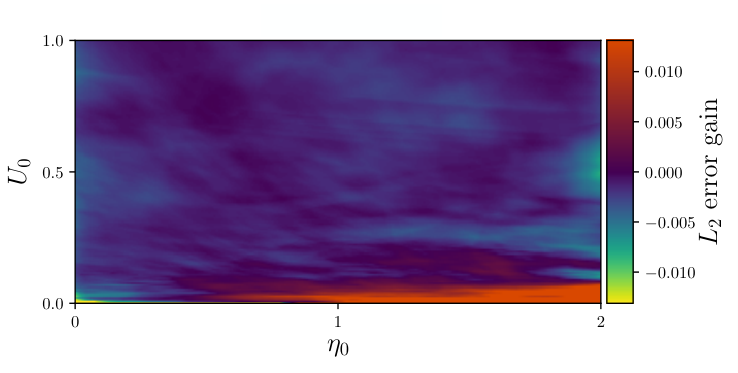
The highest error reduction occurs in the expected region. Indeed, more points are sampled where is higher. The error is slightly increased in the rest of , which could be explained by a sparser sampling on this region. However, as summarized in Table 2, the average error loss (AEL) of TBS is around six times lower than the average error gain (AEG), with and where . In practice, AEG and AEL are estimated using uniform grid integration, and averaged on the experiments.
3 Generalization of Taylor based Sampling
The previous section empirically validated the intuition behind the construction of a new, more efficient training distribution . However, this new distribution cannot always be applied as-is for two reasons. Problem 1: cannot be evaluated since it requires to compute the derivatives of , and it assumes that is differentiable, which is often not true. Moreover, the previously described setting, in which we focus on derivatives, is not suited to classification tasks where the notion of derivatives is not straightforward. Problem 2: even if could be computed and new points sampled, we could not obtain their labels to complete the training data set. In this section, we alleviate this concern to be able to use insights from in practice.
3.1 From Taylor expansion to local variance
To overcome problem 1, we construct a new metric based on statistical estimation. In this paragraph, but . The following derivations can be extended to by applying it to element-wise and then taking the sum across the dimensions.
Lemma 3.1.
Let with and the identity matrix of dimension . Let . Then,
The demonstration can be found in Appendix A. Using the unbiased estimator of variance, we thus define new indices by
| (3) |
with samples of . The metric and , so is a biased estimator of , with bias . Hence, when , becomes an unbiased estimator of . It is possible to compute from any set of points centered around . Therefore, we evaluate for each using the set of -nearest neighbors of . We note this metric , where we replace by , the values of for the neighbors of () and by , the average of on the neighbors of :
| (4) |
Equation (4) has several practical advantages. First, can even be applied to non-differentiable functions and for classification problems, unlike equation (2). Second, the definition of does not rely on , unlike equation (3). To compute , all we need are , the points used for the training of the neural network. In addition, equation (4) can even be applied when the data points are too sparse for the nearest neighbors of to be considered as close to , which is almost always the case in high dimension. It can thus be seen as a generalization of , which tends towards locally.
3.2 From sampling to weighting
To tackle problem 2, recall that the goal of the training is to find , with . With the new distribution based on previous derivations, the procedure is different. Since the training points are sampled using , we no longer minimize , but , with the new distribution. However, estimates
Let , be the pdfs of and (note that ). Then,
The straightforward Monte Carlo estimator for this expression of is
| (5) |
Thus, can be estimated with the same points as by weighting them with .
The expression of involves , the distribution of the data. Just like for , we do not have access to . The estimation of is a challenging task by itself, and standard density estimation techniques such as K-nearest neighbors or Gaussian Mixture density estimation led to extreme estimated values of in our experiments. Therefore, we decided to only apply as a first-order approximation. In practice, we re-scale the weights between and , a hyperparameter, and then divide them by their sum to avoid affecting the learning rate.
As a result, we obtain a new methodology based on weighting the training data set. We call this methodology Variance Based Sample Weighting (VBSW).
4 Variance Based Sample Weighting
In this part, we sum up Variance Based Sample Weighting (VBSW) to clarify its application to machine learning problems. We also study this methodology through toy experiments.
4.1 Methodology
Variance Based Samples Weighting (VBSW) is recapitulated in Algorithm 2. Line 1: and are hyperparameters that can be chosen jointly with all other hyperparameters, e.g. using a random search. Their effects and interactions are studied and discussed in Sections 4.2 and 5.4. Line 2-3: equation (4) is applied to compute the weights that are used to weight the data set. Notations denote that each is weighted by . To perform a nearest-neighbors search, we use an approximate nearest neighbor search technique called hierarchical navigable small world graphs [36] implemented by nmslib [10]. Line 4: Train on the weighted data set.
4.2 Toy experiments & hyperparameter study
VBSW is studied on a Double Moon (DM) classification problem, the Boston Housing (BH) regression, and Breast Cancer (BC) classification data sets.


For DM, Figure 4(b) shows that the points with higher (in red) are close to the boundary between the two classes. Indeed, in classification, VBSW can be interpreted as a local label agreement. This behavior verifies recent findings of [52] where authors conclude that in classification, a good set of weights would put importance on points close to the decision boundary.
We train a Multi-Layer Perceptron of layer of units, using Stochastic Gradient Descent (SGD) and binary cross-entropy loss function, on a points training data set for random seeds. In this experiment, VBSW, i.e. weighting the data set with is compared to the baseline where no weights are applied. The results of Table 3 show the improvement obtained with VBSW.
| VBSW | baseline | |
|---|---|---|
| DM | 99.4, | , |
| BH | 13.31, | , |
| BC | 99.12, | , |
For BH data set, a linear model is trained, and for BC data set, an MLP of layer and units, with a train-validation split of . Both models are trained with Adam [27]. Since these data sets are small and the models are light, we study the effects of and on the error. Moreover, BH is a regression task and BC a classification task, so it allows studying the effect of hyperparameters more extensively.
For BH and BC experiments, we conduct a grid search for VBSW on the values of and . As a reminder, is the ratio between the highest and the lowest weights, and is the number of neighbor points used to compute the local variance. We train a linear model for BH and a MLP with units for BC with VBSW on a grid of values of equally distributed between and and values of equally distributed between and . As a result, we train the model on pairs of values and with different random seeds for each pair.


These experiments, illustrated in Figure 5 show that the influence of and on the performances of the model can be different. For BH data set, low values of clearly lead to poorer performances. Hyperparameter seems to have less impact, although it should be chosen not too far from its lowest value, . For BC data set, on the contrary, the best performances are obtained for low values of , while a high value could be chosen for . These experiments highlight that the impact of and can be different between classification and regression, but it could also be different depending on the data set. Hence, we recommend considering these hyperparameters like many others involved in deep learning, selecting their values using hyperparameters optimization techniques.
It also shows that many different pairs lead to error improvement. It suggests that the weights approximation does not have to be exact for VBSW to be effective, as stated in Section 5.4.
4.3 Cost efficiency of VBSW
VBSW’s computational burden mostly relies on the complexity of the nearest neighbor search algorithm, which is independent and can be used as a third-party algorithm. When the data set is not too large, classical techniques like KDtree [7] can be used. However, when the number of points and the dimension of the data set increase, approximate nearest neighbors searches may be necessary to keep satisfying performances. In the previous examples, KDtree is more than sufficient. However, since we deal with more complex examples in the following, we directly use nmslib [10], an approximate nearest neighbors search library for homogeneity of the implementation.
5 VBSW for deep learning
The high dimensionality of many deep learning problems makes VBSW difficult to apply in the form previously described. In this part, we adapt VBSW to such problems and study its application to various real-world learning tasks. We also study the robustness of VBSW and its complementarity with other similar techniques.
5.1 Methodology
We mentioned that local variance could be computed using already existing points. This statement implies finding the nearest neighbors of each point. In extremely high-dimensional spaces like image spaces, the curse of dimensionality makes nearest neighbors vacuous. In addition, the data structure may be highly irregular, and the concept of nearest neighbor may be misleading. Thus, it would be irrelevant to evaluate directly on this data.
One of the strengths of deep learning is to construct good representations of the data embedded in lower-dimensional latent spaces. For instance, in Computer Vision, convolutional neural networks’ deeper layers represent more abstract features. We could leverage this representational power of neural networks and simply apply our methodology within this latent feature space.
Variance Based Samples Weighting (VBSW) for deep learning is recapitulated in Algorithm 3. Here, is the initial neural network whose feature space will be used to project the training data set and apply VBSW. Line 1: and are hyperparameters that can be chosen jointly with all other hyperparameters, e.g. using a random search. Their effects and interactions are studied and discussed in Sections 4.2 and 5.4. Line 2: The initial neural network, , is trained as usual. Notations is equivalent to , because all the weights are the same (). Line 3: The last fully connected layer is discarded, resulting in a new model , and the training data set is projected in the feature space. Line 4-5: equation (4) is applied to compute the weights that are used to weight the projected data set. Line 6: The last layer is re-trained (which is often equivalent to fitting a linear model) using the weighted data set and added to to obtain the final model . As a result, is a composition of the already trained model and trained using the weighted data set.
5.2 Image Classification
In this section, we study the performances of VBSW on MNIST [32] and Cifar10 [29] image classification data sets. For MNIST, we train LeNet [31], with different random seeds, and then apply VBSW for different random seeds, with Adam optimizer and categorical cross-entropy loss. Note that in the following, Adam is used with the default parameters of its keras implementation. We record the best value obtained from the VBSW training. We follow the same procedure for Cifar10, except that we train a ResNet20 for random seeds and with data augmentation and learning rate decay. The networks have been trained on 4 Nvidia K80 GPUs. The values of the hyperparameters used can be found in Appendix B. We compare the test accuracy between LeNet 5 + VBSW, ResNet20 + VBSW, and the initial test accuracies of LeNet 5 and ResNet20 (baseline) for each of the initial networks.
| VBSW | baseline | gain per model | |
|---|---|---|---|
| MNIST | 99.09, | , | 0.15, |
| Cifar10 | 91.30, | , | 1.65, |
The results statistics are gathered in Table 4, which also displays statistics about the gain due to VBSW for each model. The results on MNIST are slightly but consistently better than for the baseline, by for the best with up to of accuracy gain per model. For Cifar10, we get a accuracy improvement for the best model and up to accuracy gain, meaning that among the ResNet20s, there is one whose accuracy has been improved by using VBSW. Note that applying VBSW took less than 15 minutes on a laptop with an i7-7700HQ CPU. A visualization of the samples weighted by the highest is given in Figure 6.

5.3 Text Classification and Regression
In this section, we study the performances of VBSW on RTE and MRPC, two text classification data sets, and STS-B, a text classification data set, extracted from the glue benchmark [51]. For this application, we use Bert, a modern neural network based on transformers [50] that is the state-of-the-art of text-based machine learning tasks. We do not pre-train Bert, like in the previous experiments, since it has been originally built for Transfer Learning purposes. Therefore, its purpose is to be used as-is and then fine-tuned on any text data set see [14]. However, because of the small size of the data set and the high number of model parameters, we chose not to fine-tune the Bert model and only to use the representations of the data sets in its feature space to apply VBSW. More specifically, we use tiny-bert [49], which is a lighter version of the initial Bert. We train the linear model with TensorFlow to be able to add the trained model on top of the Bert model and obtain a unified model. RTE and MRPC are classification tasks, so we use binary cross-entropy loss function to train our models. STS-B is a regression task, so the model is trained with Mean Squared Error. All the models are trained with Adam optimizer. For each task, we compare the training of the linear model with VBSW and without VBSW (baseline). The results obtained with VBSW are better overall, except for Pearson Correlation in STS-B, which is slightly worse than baseline (Table 5).
| VBSW | baseline | |||
| m1 | m2 | m1 | m2 | |
| RTE | 61.73, | - | , | - |
| STS-B | 62.31, | 60.99, | , | , |
| MRPC | 72.30, | 82.64, | , | , |
5.4 Robustness of VBSW
In this section, we assess the robustness of VBSW. First, we focus on the robustness to label noise. To that end, we train a ResNet20 on Cifar10 with four different noise levels. We randomly change the label of training points for four different values of (, , and ). We then apply VBSW times and evaluate the obtained neural networks on a clean test set. The results are gathered in Table 6.
| noise | ||||
|---|---|---|---|---|
| original error | ||||
| VBSW | 87.76, | 86.03, | 84.35, | 82.48, |
The results show that VBSW is still effective despite label noise. This specificity must be related to the robustness of VBSW with respect to the choice of hyperparameters and , as seen in Section 4.2. Indeed, it shows that many combinations of and improves the performances of the neural network, and therefore that VBSW is actually robust to error in the weights evaluation. Its robustness to label noise hence stems from its robustness to weights evaluation error, since label noise essentially hurts the accuracy of the weights evaluation.
Although VBSW is robust to label noise, note that the goal of VBSW is not to address noisy label problem, like discussed in Section 1. It may be more effective to use a sampling technique tailored specifically for this situation.
5.5 Complementarity of VBSW
Existing techniques based on dataset processing can be used jointly with VBSW, by applying the first technique during the initial training of the neural network and then applying VBSW on its feature space. To illustrate this specificity, we compare VBSW with the recently introduced Active Bias (AB) [11] and transfer-learning-based curriculum learning (TCL) [18]. AB dynamically weights the samples based on the variance of the probability of prediction of each point throughout the training, and TCL creates a curriculum based on sample difficulty evaluated on previously trained neural networks. Here, we study the effects of AB and TCL combined with VBSW for the training of a ResNet20 on Cifar10. Table 7 gathers the results of experiments for different baselines: vanilla, for regular training with Adam optimizer, AB / TCL for training with AB / TCL, VBSW for the application of VBSW on top of regular training, and VBSW + AB / VBSW + CL for initial training with AB / TCL and the application of VBSW. Unlike in Section 5.2, we do not use data augmentation nor learning rate decay in order to simplify the experiments.
| accuracy () | VBSW gpm | |
|---|---|---|
| vanilla | , | - |
| AB | , | - |
| TCL | , | - |
| VBSW | , | , |
| AB + VBSW | , | , |
| TCL + VBSW | , | , |
The accuracy obtained with VBSW is quite similar to AB. While TCL yields better results than VBSW alone, the best accuracy is obtained when they are used jointly. Overall, the best neural networks are obtained when AB and TCL are used along with VBSW (AB + VBSW and TCL + VBSW), which demonstrates the complementarity of VBSW with other dataset processing techniques. Note that VBSW works much better when applied to a neural network initially trained with TCL. It means that TCL creates neural network features particularly suited to VBSW. This lead might be explored in future works.
6 Discussion and Perspectives
By studying the training distribution of the neural network, we explored a practical and classical question that naturally arises when performing surrogate modeling for approximating computer codes: how to construct the training set? We found that exploring this question led to findings that are also relevant for approximation theory, which is an important component of machine learning.
Hence, the results obtained in this paper are impactful both for machine learning in numerical simulations and machine learning in general.
6.1 Impact for numerical simulations
This work comes from the observation that, on our approximation problems, neural networks are more efficient when more data are sampled where the function to learn is steeper. It is an attempt to formalize this observation and to construct a workable methodology out of it. As a result, the methodologies for constructing the distribution can be used as new, principled designs of experiments.
In the context of numerical simulations, once is constructed, it is possible to sample new data from it. It alleviates Problem 2, described in Section 3.2. In theory, Problem 1 is also solved since we could have access to the derivatives - either by instrumenting the code with automatic differentiation if we have access to its implementation or by estimating them with finite differences. However, the implementation of automatic differentiation can be tedious, and if the computer code is slow and high dimensional, finite differences may be unaffordable. In that case, it is possible to use a third methodology based on the approximation of using local variance, like VBSW, and the sampling of new points, like TBS.
Finally, the method allows improving the error of neural networks without increasing the computational cost of their prediction. This achievement is of interest when they are intended to accelerate numerical simulations.
6.2 Impact for machine learning
VBSW is validated on several tasks, complementary with other training distribution modification frameworks, and robust to noise. It makes it quite versatile. Moreover, the problem of high dimensionality and irregularity of , which often arises in deep learning problems, is alleviated by focusing on the latent space of neural networks. This makes VBSW scalable. As a result, VBSW can be applied to complex neural networks such as ResNet, or Bert, for various machine learning tasks.
The experiments support an original view of the learning problem that involves the local variations of . The studies of Section 2.2, that use the derivatives of the function to learn to sample a more efficient training data set, support this approach as well. This view is also bolstered up by conclusions of [52]. VBSW allows extending this original view to problems where the derivatives of are not accessible and sometimes not defined. Indeed, VBSW comes from Taylor expansion, which is specific to differentiable functions, but in the end, it can be applied regardless of the properties of .
Finally, this method is cost-effective. In most cases, it allows to quickly improve the performances of a neural network using a regular CPU. It is better than carrying on entirely new training with a wider and deeper neural network.
6.3 Further studies
Although VBSW uses theoretically justified approximations concerning TBS, the actual effect of these approximations should be more thoroughly investigated. For instance, we could further study the impact of not explicitly using , the data distribution, in the weights definitions; the convergence of the estimator of , and in which context it is adequately approximated; and a more generic derivative-based generalization bound. In addition, VBSW demonstrated intriguing behaviors, like its impressive synergy with TCL [18], which would deserve more attention.
7 Conclusion
This work is based on the observation that, in supervised learning, a function is more difficult to approximate by a neural network in the regions where it is steep. We mathematically traduced this intuition, derived a generalization bound to illustrate it, and a methodology, Taylor Based Sampling, to test it empirically. In order to be able to use these insights for machine learning problems where is not available, we constructed a weighting scheme, Variance Based Samples Weighting (VBSW) that uses the variance of the training samples’ labels to weight the training data set. VBSW is simple to use and implement because it only requires computing statistics on the input space. In Deep Learning, applying VBSW on the data set projected in an already trained neural network feature space allows reducing its error by simply re-training its last layer. Although specifically investigated in deep learning, this method applies to any loss-function-based supervised learning problem and is scalable, cost-effective, robust, and versatile. It is validated on several applications, such as glue benchmark with bert for text classification and regression, and Cifar10 with ResNet for image classification.
Appendix A Appendix A: Proofs
A.1 Illustration of the link using derivatives
(Section 2.1)
We look at approximating , , with a NN . The goal of the approximation problem can be seen as being able to generalize to points not seen during the training. We thus want the generalization error to be as small as possible. Given an initial data set drawn from and , and the loss function being the squared error, recall that the integrated error , its estimation and the generalization error can be written:
| (6) |
where denotes the squared norm. In the following, we find an upper bound for . We start by finding an upper bound for and then for using equation (6).
Let , be some sub-spaces of a bounded space such that , Ø, and . Then,
Suppose that ( becomes and becomes x) and twice differentiable. Let . The volume since is a probability measure, and therefore for all . Using Taylor expansion at order 2, and since for all
To find an upper bound for , we can first find an upper bound for , with .
NN is Lipschitz, so since is bounded (so are ), for all , . Hence,
And finally, using triangular inequality,
Now, being the squared norm:
Hornik’s theorem [20] states that given a norm such that , with a probability measure, for any , there exists such that for a Multi Layer Perceptron, , ,
This theorem grants that for any , with , there exists such that
| (7) |
Let’s introduce such that . Note that for any , is . Now, let’s choose such that is . Then, equation (7) implies that
Thus, we have and therefore,
Finally,
| (8) |
We see that on the regions where is higher, quantity (the volume of ) has a stronger impact on the GB. Then, since can be seen as a metric for the local density of the data set (the smaller is, the denser the data set is), the Generalization Bound (GB) can be reduced more efficiently by adding more points around in these regions. This bound also involves , the Lipschitz constant of the NN, which has the same impact as . It also illustrates the link between the Lipschitz constant and the generalization error, which has been pointed out by several works like, for instance, [17], [3] and [43].
A.2 Problem 1: Unavailability of derivatives
(Section 3.1)
In this paragraph, we consider but . The following derivations can be extended to by applying it to element-wise. Let with , , i.e. and . Using Taylor expansion on at order gives
with and the gradient and the Hessian of w.r.t. . We now compute and make appear in its expression to establish a link between these two quantities:
Since , and with the cross derivatives of w.r.t. and ,
In this expression, three quantities have to be assessed : , and .
First, since are i.i.d.,
To assess , three cases have to be considered.
- •
If , because ,
- •
If or (we consider , and the result holds for by commutativity),
- •
If and , and are independent and so = 0.
Finally, to assess , four cases have to be considered:
- •
If ,
- •
If and , since and are independent.
- •
If and ,
- •
If and ,
All other possible cases can be assessed using the previous results, commutativity and symmetry of operator. Hence,
And finally,
| (9) |
Appendix B Appendix B: Hyperparameters spaces
The values chosen for the hyperparameters experiments are gathered in Table 8. For Adam optimizer hyperparameters, we kept the default values of Keras implementation. We chose these hyperparameters after simple grid searches.
| Experiment | learning rate | batch size | epochs | optimizer | random seeds | ||
|---|---|---|---|---|---|---|---|
| double moon | 100 | 20 | 100 | 10000 | SGD | 50 | |
| Boston housing | 8 | 35 | 404 | 50000 | Adam | 10 | |
| Breast Cancer | 50 | 35 | 455 | 250000 | Adam | 10 | |
| MNIST | 40 | 20 | 25 | 25 | Adam | 40 | |
| Cifar10 | 40 | 20 | 25 | 25 | Adam | 50 | |
| RTE | 20 | 10 | 8 | 10000 | Adam | 50 | |
| STS-B | 30 | 30 | 8 | 10000 | Adam | 50 | |
| MRPC | 75 | 25 | 16 | 10000 | Adam | 50 |
References
- [1] Martín Abadi, Ashish Agarwal, Paul Barham, Eugene Brevdo, Zhifeng Chen, Craig Citro, Greg S. Corrado, Andy Davis, Jeffrey Dean, Matthieu Devin, Sanjay Ghemawat, Ian Goodfellow, Andrew Harp, Geoffrey Irving, Michael Isard, Yangqing Jia, Rafal Jozefowicz, Lukasz Kaiser, Manjunath Kudlur, Josh Levenberg, Dan Mané, Rajat Monga, Sherry Moore, Derek Murray, Chris Olah, Mike Schuster, Jonathon Shlens, Benoit Steiner, Ilya Sutskever, Kunal Talwar, Paul Tucker, Vincent Vanhoucke, Vijay Vasudevan, Fernanda Viégas, Oriol Vinyals, Pete Warden, Martin Wattenberg, Martin Wicke, Yuan Yu, and Xiaoqiang Zheng. TensorFlow: Large-scale machine learning on heterogeneous systems, 2015. Software available from tensorflow.org.
- [2] Sanjeev Arora, Rong Ge, Behnam Neyshabur, and Yi Zhang. Stronger generalization bounds for deep nets via a compression approach. In Jennifer Dy and Andreas Krause, editors, Proceedings of the 35th International Conference on Machine Learning, volume 80 of Proceedings of Machine Learning Research, pages 254–263, Stockholmsmässan, Stockholm Sweden, 10–15 Jul 2018. PMLR.
- [3] Peter L Bartlett, Dylan J Foster, and Matus J Telgarsky. Spectrally-normalized margin bounds for neural networks. In I. Guyon, U. V. Luxburg, S. Bengio, H. Wallach, R. Fergus, S. Vishwanathan, and R. Garnett, editors, Advances in Neural Information Processing Systems 30, pages 6240–6249. Curran Associates, Inc., 2017.
- [4] Peter L. Bartlett, Nick Harvey, Christopher Liaw, and Abbas Mehrabian. Nearly-tight vc-dimension and pseudodimension bounds for piecewise linear neural networks. Journal of Machine Learning Research, 20(63):1–17, 2019.
- [5] Peter L. Bartlett, Vitaly Maiorov, and Ron Meir. Almost linear vc dimension bounds for piecewise polynomial networks. In Proceedings of the 11th International Conference on Neural Information Processing Systems, NIPS’98, page 190–196, Cambridge, MA, USA, 1998. MIT Press.
- [6] Yoshua Bengio, Jérôme Louradour, Ronan Collobert, and Jason Weston. Curriculum learning. In Proceedings of the 26th Annual International Conference on Machine Learning, ICML ’09, pages 41–48, New York, NY, USA, 2009. ACM.
- [7] Jon Louis Bentley. Multidimensional binary search trees used for associative searching. Commun. ACM, 18(9):509–517, September 1975.
- [8] Adrien Bernède and Gaël Poëtte. An unsplit monte-carlo solver for the resolution of the linear boltzmann equation coupled to (stiff) bateman equations. Journal of Computational Physics, 354:211–241, 02 2018.
- [9] M. Bisi and L. Desvillettes. From reactive boltzmann equations to reaction–diffusion systems. Journal of Statistical Physics, 124(2):881–912, Aug 2006.
- [10] Leonid Boytsov and Bilegsaikhan Naidan. Engineering efficient and effective non-metric space library. In Nieves R. Brisaboa, Oscar Pedreira, and Pavel Zezula, editors, Similarity Search and Applications - 6th International Conference, SISAP 2013, A Coruña, Spain, October 2-4, 2013, Proceedings, volume 8199 of Lecture Notes in Computer Science, pages 280–293. Springer, 2013.
- [11] Haw-Shiuan Chang, Erik Learned-Miller, and Andrew McCallum. Active bias: Training more accurate neural networks by emphasizing high variance samples. In I. Guyon, U. V. Luxburg, S. Bengio, H. Wallach, R. Fergus, S. Vishwanathan, and R. Garnett, editors, Advances in Neural Information Processing Systems 30, pages 1002–1012. Curran Associates, Inc., 2017.
- [12] David A. Cohn. Neural Network Exploration Using Optimal Experiment Design. Neural Networks, 9(6):1071–1083, August 1996.
- [13] Yin Cui, Menglin Jia, Tsung-Yi Lin, Yang Song, and Serge Belongie. Class-balanced loss based on effective number of samples. In The IEEE Conference on Computer Vision and Pattern Recognition (CVPR), June 2019.
- [14] Jacob Devlin, Ming-Wei Chang, Kenton Lee, and Kristina Toutanova. BERT: Pre-training of deep bidirectional transformers for language understanding. In Proceedings of the 2019 Conference of the North American Chapter of the Association for Computational Linguistics: Human Language Technologies, Volume 1 (Long and Short Papers), pages 4171–4186, Minneapolis, Minnesota, June 2019. Association for Computational Linguistics.
- [15] Jan Dufek, Dan Kotlyar, and Eugene Shwageraus. The stochastic implicit euler method – a stable coupling scheme for monte carlo burnup calculations. Annals of Nuclear Energy, 60:295 – 300, 10 2013.
- [16] Yarin Gal, Riashat Islam, and Zoubin Ghahramani. Deep bayesian active learning with image data. In Proceedings of the 34th International Conference on Machine Learning - Volume 70, ICML’17, pages 1183–1192. JMLR.org, 2017.
- [17] Henry Gouk, Eibe Frank, Bernhard Pfahringer, and Michael Cree. Regularisation of neural networks by enforcing lipschitz continuity. 04 2018.
- [18] Guy Hacohen and Daphna Weinshall. On the power of curriculum learning in training deep networks. In Kamalika Chaudhuri and Ruslan Salakhutdinov, editors, Proceedings of the 36th International Conference on Machine Learning, volume 97 of Proceedings of Machine Learning Research, pages 2535–2544. PMLR, 09–15 Jun 2019.
- [19] Kaiming He, Xiangyu Zhang, Shaoqing Ren, and Jian Sun. Deep residual learning for image recognition. 2016 IEEE Conference on Computer Vision and Pattern Recognition (CVPR), pages 770–778, 2015.
- [20] Kurt Hornik, Maxwell Stinchcombe, and Halbert White. Multilayer feedforward networks are universal approximators. Neural Networks, 2(5):359 – 366, 1989.
- [21] Daniel Jakubovitz, Raja Giryes, and Miguel R. D. Rodrigues. Generalization error in deep learning. CoRR, abs/1808.01174, 2018.
- [22] Lu Jiang, Deyu Meng, Qian Zhao, Shiguang Shan, and Alexander G. Hauptmann. Self-paced curriculum learning. In Proceedings of the Twenty-Ninth AAAI Conference on Artificial Intelligence, AAAI’15, page 2694–2700. AAAI Press, 2015.
- [23] Tang Jie and Pieter Abbeel. On a connection between importance sampling and the likelihood ratio policy gradient. In J. D. Lafferty, C. K. I. Williams, J. Shawe-Taylor, R. S. Zemel, and A. Culotta, editors, Advances in Neural Information Processing Systems 23, pages 1000–1008. Curran Associates, Inc., 2010.
- [24] M.E. Johnson, L.M. Moore, and D. Ylvisaker. Minimax and maximin distance designs. Journal of Statistical Planning and Inference, 26(2):131–148, October 1990.
- [25] Donald R. Jones, Matthias Schonlau, and William J. Welch. Efficient global optimization of expensive black-box functions. Journal of Global Optimization, 13(4):455–492, Dec 1998.
- [26] Angelos Katharopoulos and François Fleuret. Not all samples are created equal: Deep learning with importance sampling. In ICML, 2018.
- [27] Diederik P. Kingma and Jimmy Ba. Adam: A method for stochastic optimization. In ICLR (Poster), 2015.
- [28] Ksenia Konyushkova, Raphael Sznitman, and Pascal Fua. Learning active learning from data. In I. Guyon, U. V. Luxburg, S. Bengio, H. Wallach, R. Fergus, S. Vishwanathan, and R. Garnett, editors, Advances in Neural Information Processing Systems 30, pages 4225–4235. Curran Associates, Inc., 2017.
- [29] Alex Krizhevsky. Learning multiple layers of features from tiny images. Technical report, 2009.
- [30] M. P. Kumar, Benjamin Packer, and Daphne Koller. Self-paced learning for latent variable models. In J. D. Lafferty, C. K. I. Williams, J. Shawe-Taylor, R. S. Zemel, and A. Culotta, editors, Advances in Neural Information Processing Systems 23, pages 1189–1197. Curran Associates, Inc., 2010.
- [31] Y. Lecun, L. Bottou, Y. Bengio, and P. Haffner. Gradient-based learning applied to document recognition. Proceedings of the IEEE, 86(11):2278–2324, 1998.
- [32] Yann LeCun and Corinna Cortes. MNIST handwritten digit database. 2010.
- [33] Tongliang Liu and Dacheng Tao. Classification with noisy labels by importance reweighting. IEEE Trans. Pattern Anal. Mach. Intell., 38(3):447–461, March 2016.
- [34] D. Lucor, C. Enaux, H. Jourdren, and P. Sagaut. Stochastic design optimization: Application to reacting flows. Computer Methods in Applied Mechanics and Engineering, 196(49):5047 – 5062, 2007.
- [35] David J. C. MacKay. Information-Based Objective Functions for Active Data Selection. Neural Computation, 4(4):590–604, July 1992.
- [36] Yu A. Malkov and D. A. Yashunin. Efficient and Robust Approximate Nearest Neighbor Search Using Hierarchical Navigable Small World Graphs. IEEE Transactions on Pattern Analysis and Machine Intelligence, 42(4):824–836, April 2020.
- [37] Tambet Matiisen, Avital Oliver, Taco Cohen, and John Schulman. Teacher–student curriculum learning. IEEE Transactions on Neural Networks and Learning Systems, 31:3732–3740, 2020.
- [38] M. D. McKay, R. J. Beckman, and W. J. Conover. A Comparison of Three Methods for Selecting Values of Input Variables in the Analysis of Output from a Computer Code. Technometrics, 21(2):239, May 1979.
- [39] Behnam Neyshabur, Srinadh Bhojanapalli, David Mcallester, and Nati Srebro. Exploring generalization in deep learning. In I. Guyon, U. V. Luxburg, S. Bengio, H. Wallach, R. Fergus, S. Vishwanathan, and R. Garnett, editors, Advances in Neural Information Processing Systems 30, pages 5947–5956. Curran Associates, Inc., 2017.
- [40] Behnam Neyshabur, Srinadh Bhojanapalli, and Nathan Srebro. A PAC-bayesian approach to spectrally-normalized margin bounds for neural networks. In International Conference on Learning Representations, 2018.
- [41] F. Pedregosa, G. Varoquaux, A. Gramfort, V. Michel, B. Thirion, O. Grisel, M. Blondel, P. Prettenhofer, R. Weiss, V. Dubourg, J. Vanderplas, A. Passos, D. Cournapeau, M. Brucher, M. Perrot, and E. Duchesnay. Scikit-learn: Machine learning in Python. Journal of Machine Learning Research, 12:2825–2830, 2011.
- [42] Benoit Perthame. Transport Equations in Biology. 01 2007.
- [43] Haifeng Qian and Mark N. Wegman. L2-nonexpansive neural networks. In International Conference on Learning Representations, 2019.
- [44] Mengye Ren, Wenyuan Zeng, Bin Yang, and Raquel Urtasun. Learning to reweight examples for robust deep learning. CoRR, abs/1803.09050, 2018.
- [45] S. Seo, M. Wallat, T. Graepel, and K. Obermayer. Gaussian process regression: Active data selection and test point rejection. In Proceedings of the International Joint Conference on Neural Networks, 2000.
- [46] Burr Settles. Active Learning. Synthesis Lectures on Artificial Intelligence and Machine Learning. Morgan & Claypool Publishers, 2012.
- [47] M. C. Shewry and H. P. Wynn. Maximum entropy sampling. Journal of Applied Statistics, 14(2):165–170, January 1987.
- [48] Abhinav Shrivastava, Abhinav Gupta, and Ross B. Girshick. Training region-based object detectors with online hard example mining. CoRR, abs/1604.03540, 2016.
- [49] Iulia Turc, Ming-Wei Chang, Kenton Lee, and Kristina Toutanova. Well-read students learn better: On the importance of pre-training compact models. arXiv preprint arXiv:1908.08962v2, 2019.
- [50] Ashish Vaswani, Noam Shazeer, Niki Parmar, Jakob Uszkoreit, Llion Jones, Aidan N Gomez, Ł ukasz Kaiser, and Illia Polosukhin. Attention is all you need. In I. Guyon, U. V. Luxburg, S. Bengio, H. Wallach, R. Fergus, S. Vishwanathan, and R. Garnett, editors, Advances in Neural Information Processing Systems 30, pages 5998–6008. Curran Associates, Inc., 2017.
- [51] Alex Wang, Amanpreet Singh, Julian Michael, Felix Hill, Omer Levy, and Samuel R. Bowman. GLUE: A multi-task benchmark and analysis platform for natural language understanding. In International Conference on Learning Representations, 2019.
- [52] Da Xu, Yuting Ye, and Chuanwei Ruan. Understanding the role of importance weighting for deep learning. In International Conference on Learning Representations, 2021.
- [53] Huan Xu and Shie Mannor. Robustness and generalization. Machine Learning, 86(3):391–423, Mar 2012.