Stephen M. Griffies
\extraaffilNOAA/Geophysical Fluid Dynamics Laboratory and
Program in Atmospheric and Oceanic Sciences, Princeton University, Princeton, NJ, USA
On the Discrete Normal Modes of Quasigeostrophic Theory
Abstract
The discrete baroclinic modes of quasigeostrophic theory are incomplete and the incompleteness manifests as a loss of information in the projection process. The incompleteness of the baroclinic modes is related to the presence of two previously unnoticed stationary step-wave solutions of the Rossby wave problem with flat boundaries. These step-waves are the limit of surface quasigeostrophic waves as boundary buoyancy gradients vanish. A complete normal mode basis for quasigeostrophic theory is obtained by considering the traditional Rossby wave problem with prescribed buoyancy gradients at the lower and upper boundaries. The presence of these boundary buoyancy gradients activates the previously inert boundary degrees of freedom. These Rossby waves have several novel properties such as the presence of multiple modes with no internal zeros, a finite number of modes with negative norms, and their vertical structures form a basis capable of representing any quasigeostrophic state with a differentiable series expansion. Using this complete basis, we are able to obtain a differentiable series expansion to the potential vorticity of Bretherton (with Dirac delta contributions). We also examine the quasigeostrophic vertical velocity modes and derive a complete basis for such modes as well. A natural application of these modes is the development of a weakly non-linear wave-interaction theory of geostrophic turbulence that takes topography into account.
1 Introduction
1.1 Background
The vertical decomposition of quasigeostrophic motion into normal modes plays an important role in bounded stratified geophysical fluids (Charney 1971; Flierl 1978; Fu and Flierl 1980; Wunsch 1997; Chelton et al. 1998; Smith and Vallis 2001; Tulloch and Smith 2009; Lapeyre 2009; Ferrari et al. 2010; Ferrari and Wunsch 2010; de La Lama et al. 2016; LaCasce 2017; Brink and Pedlosky 2019, e.g.,). Most prevalent are the traditional baroclinic modes (Vallis 2017, e.g., section 6.5.2 in) that are the vertical structures of Rossby waves in a quiescent ocean with no topography or boundary buoyancy gradients. In a landmark contribution, Wunsch 1997 partitions the ocean’s kinetic energy into the baroclinic modes and finds that the zeroth and first baroclinic modes dominate over most of the extratropical ocean. Additionally, Wunsch 1997 concludes that the surface signal primarily reflects the first baroclinic mode and, therefore, the motion of the thermocline.
However, the use of baroclinic modes has come under increasing scrutiny in recent years (Lapeyre 2009; Roullet et al. 2012; Scott and Furnival 2012; Smith and Vanneste 2012). Lapeyre 2009 observes that the vertical shear of the baroclinic modes vanishes at the boundaries, thus leading to the concomitant vanishing of the boundary buoyancy. Consequently, Lapeyre 2009 proposes that the baroclinic modes cannot be complete11 1 A collection of functions is said to be complete in some function space, , if this collection forms a basis of . Specifying the underlying function space, , turns out to be crucial, as we see in section 22.4. due to their inability to represent boundary buoyancy. To supplement the baroclinic modes, Lapeyre 2009 includes a boundary-trapped exponential surface quasigeostrophic solution (Held et al. 1995, see) and suggests that the surface signal primarily reflects, not thermocline motion, but boundary-trapped surface quasigeostrophic dynamics (Lapeyre 2017, see also).
Appending additional functions to the collections of normal modes as in Lapeyre 2009 or Scott and Furnival 2012 does not result in a set of normal modes since the appended functions are not orthogonal to the original modes. It is only with Smith and Vanneste 2012 that a set of normal modes capable of representing arbitrary surface buoyancy is derived.
Yet it is not clear how the normal modes of Smith and Vanneste 2012 differ from the baroclinic modes or what these modes correspond to in linear theory. Indeed, Rocha et al. 2015, noting that the baroclinic series expansion of any sufficiently smooth function converges uniformly to the function itself, argues that the incompleteness of the baroclinic modes has been “overstated”. Moreover, de La Lama et al. 2016 and LaCasce 2017, motivated by the observation that the leading empirical orthogonal function of Wunsch 1997 vanishes near the ocean bottom, propose an alternate set of modes—the surface modes—that have a vanishing pressure at the bottom boundary.
We thus have a variety of proposed normal modes and it is not clear how their properties differ. Are the baroclinic modes actually incomplete? What about the surface modes? What does completeness mean in this context? The purpose of this paper is to answer these questions.
1.2 Normal modes and eigenfunctions
A normal mode is a linear motion in which all components of a system move coherently at a single frequency. Mathematically, a normal mode has the form
| (1) |
where describes the spatial structure of the mode and is its angular frequency. The function is obtained by solving a differential eigenvalue problem and hence is an eigenfunction. The collection of all eigenfunctions forms a basis of some function space relevant to the problem.
By an abuse of terminology, the spatial structure, , is often called a normal mode (e.g., the term “Fourier mode” is often used for where is a wavenumber). In linear theory, this misnomer is often benign as each corresponds to a frequency . For example, given some initial condition , we decompose as a sum of modes at ,
| (2) |
where the are the Fourier coefficients, and the time evolution is then given by
| (3) |
However, with non-linear dynamics, this abuse of terminology can be confusing. Given some spatial structure, , in a fluid whose flow is non-linear, we can still exploit the basis properties of the eigenfunctions to decompose as in equation (2). Whereas in a linear fluid only wave motion of the form (1) is possible, a non-linear flow admits a larger collection of solutions (e.g., non-linear waves and coherent vortices) and so the linear wave solution (3) no longer follows from the decomposition (2).
For this reason, we call the linear solution (1) a physical normal mode to distinguish it from the spatial structure , which is only an eigenfunction. Otherwise, we will use the terms “normal mode” and “eigenfunction” interchangeably to refer to the spatial structure , as is prevalent in the literature.
Our strategy here is then the following. We find the physical normal modes [of the form (1)] to various Rossby wave problems and examine the basis properties of their constituent eigenfunctions . Our goal is to find a collection of eigenfunctions (i.e., “normal modes” in the prevalent terminology) capable of representing every possible quasigeostrophic state.
1.3 Contents of this article
This article constitutes an examination of all collections of discrete (i.e., non-continuum22 2 Continuum modes appear once a sheared mean-flow is present, e.g., Drazin et al. 1982, Balmforth and Morrison 1994; Balmforth and Morrison 1995, and Brink and Pedlosky 2019. ) quasigeostrophic normal modes. We include the baroclinic modes, the surface modes of de La Lama et al. 2016 and LaCasce 2017, the surface-aware mode of Smith and Vanneste 2012, as well as various generalizations. To study the completeness of a set of normal modes, we must first define the underlying space in question. From general considerations, we introduce in section 2 the quasigeostrophic phase space, defined as the space of all possible quasigeostrophic states. Subsequently, in section 3 we use the general theory of differential eigenvalue problems with eigenvalue dependent boundary conditions, as developed in Yassin 2021, to study Rossby waves in an ocean with prescribed boundary buoyancy gradients (e.g., topography, see section 22.1). Intriguingly, in an ocean with no topography, we find that, in addition to the usual baroclinic modes, there are two additional stationary step-mode solutions that have not been noted before. The stationary step-modes are the limits of boundary-trapped surface quasigeostrophic waves as the boundary buoyancy gradient vanishes.
Our study of Rossby waves then leads us examine all possible discrete collections of normal modes in section 4. As shown in this section, the baroclinic modes are incomplete, as argued by Lapeyre 2009, and we point out that the incompleteness leads to a loss of information after projecting a function onto the baroclinic modes. In contrast, modes such as those suggested by Smith and Vanneste 2012 are complete in the quasigeostrophic phase space so that projecting a function onto such modes provides an equivalent representation of the function.
We offer discussion of our analysis in Section 5 and conclusions in Section 6. Appendix A summarizes the key mathematical results pertaining to eigenvalue problems where the eigenvalue appears in the boundary conditions. Appendix B then summarizes the polarization relations as well as the vertical velocity eigenvalue problem.
2 Mathematics of the quasigeostrophic phase space
2.1 The potential vorticity
Consider a three-dimensional region of the form
| (4) |
The area of the lower and upper boundaries is denoted by and is a rectangle of area while (lower boundary) and (upper boundary) are constants. The horizontal boundaries are either rigid or periodic.
The state of a quasigeostrophic fluid in is determined by a charge-like quantity known as the quasigeostrophic potential vorticity (Hoskins et al. 1985; Schneider et al. 2003). If the potential vorticity is distributed throughout the three-dimensional region , we are concerned with the volume potential vorticity density, , with related to the geostrophic streamfunction by [e.g., section 5.4 of Vallis 2017]
| (5) |
Here, the latitude dependent Coriolis parameter is
| (6) |
is the prescribed background buoyancy frequency, is the horizontal Laplacian operator, and
| (7) |
is the horizontal geostrophic velocity, .
Additionally, the potential vorticity may be distributed over a two-dimensional region, say the lower and upper boundaries , to obtain surface potential vorticity densities and . The surface potential vorticity densities are related to the streamfunction by
| (8) |
where is an imposed surface potential vorticity density at the lower or upper boundary and . The density corresponds to a prescribed buoyancy
| (9) |
at the th boundary [see equation (106)]. Alternatively, may be thought of as an infinitesimal topography through
| (10) |
where represents infinitesimal topography at the th boundary. Whereas has dimensions of inverse time, has dimensions of length per time.
2.2 Defining the quasigeostrophic phase space
We define the quasigeostrophic phase space to be the space of all possible quasigeostrophic states, with a quasigeostrophic state determined by the potential vorticity densities, , and . Note that the volume potential vorticity density, , is defined throughout the whole fluid region , so that . In contrast, the surface potential vorticity densities, and , are only defined on the two-dimensional lower and upper boundary surfaces, , so that .
It is useful to restate the previous paragraph with some added mathematical precision. For that purpose, let be the space of square-integrable functions33 3 The definition of is more subtle than presented here. Namely, elements of are not functions, but rather equivalence classes of functions leading to the unintuitive properties seen in this section. See Yassin 2021 and citations within for more details. in the fluid volume , and let be the space of square-integrable functions on the boundary area . Elements of are functions of three spatial coordinates whereas elements of are functions of two spatial coordinates. Hence, and .
Define the space by
| (11) |
where is the direct sum. Equation (11) states that any element of is a tuple of three functions, where is a function on the volume and hence element of , while the functions , for , are functions on the area and hence are elements of . We conclude that and that is the space of all possible quasigeostrophic states. We thus call the quasigeostrophic phase space.
2.3 The phase space in terms of the streamfunction
Given an element , we can reconstruct a continuous function that contains the same dynamical information as . By inverting the problem
| (12) | ||||
we obtain a function that is unique up to a gauge transformation (Schneider et al. 2003, see). Conversely, given a function , we can differentiate as in equations (12) to obtain . Thus, we can also consider the quasigeostrophic phase space to be the space of all possible streamfunctions .
Equations (12) motivate the definition of the relative potential vorticity densities, and , which are the portions of the potential vorticity providing a source for a streamfunction. Explicitly, the relative potential vorticity densities are
| (13a) | ||||||
| (13b) | ||||||
| (13c) | ||||||
2.4 The vertical structure phase space
Since the fluid region, , is separable, we can expand the potential vorticity density distribution, , and the streamfunction in terms of the eigenfunctions, , of the horizontal Laplacian. For a horizontal domain , the eigenfunction satisfies
| (14) |
where is the horizontal position vector, is the horizontal wavevector, and is the horizontal wavenumber. For example, in a horizontally periodic domain the eigenfunctions are proportional to complex exponentials, .
Projecting the relative potential vorticity density distribution, , onto the horizontal eigenfunctions, , yields
| (15a) | ||||||
| (15b) | ||||||
Thus the Fourier coefficients of are where is a function of and and are independent of . Hence, is an element of whereas and are elements of the space of complex numbers44 4 Since all physical fields must be real, only a single degree of freedom is gained from . Furthermore, when complex notation is used (e.g., complex exponentials for the horizontal eigenfunctions ) it is only the real part of the fields that is physical. , .
We conclude that the vertical structure of the potential vorticity, given by , is an element of
| (16) |
so that the vertical structures of the potential vorticity distribution are determined by a function, , in and two -independent elements, and , of . Similarly, the streamfunction can be represented as
| (17) |
where and are related by
| (18a) | |||
| (18b) | |||
As before, knowledge of the vertical structure of the streamfunction, , is equivalent to knowing the vertical structure of the potential vorticity distribution, . Thus is also the space of all possible streamfunction vertical structures.
That belongs to and not underlies much of the confusion over baroclinic modes. Assertions of completeness, based on Sturm-Liouville theory, assume that is an element of . However, as we have shown, that is an incorrect assumption. That belongs to will have consequences for the convergence and differentiability of normal mode expansions, as discussed in section 4. In the context of quasigeostrophic theory, the space first appeared in Smith and Vanneste 2012. More generally, appears in the presence of non-trivial boundary dynamics (Yassin 2021).
We call the vertical structure phase space, and for convenience we denote by for the remainder of the article. The vertical structure phase space is then written as the direct sum
| (19) |
2.5 Representing the energy and potential enstrophy
We find it convenient to represent several quadratic quantities in terms of the eigenfunctions of the horizontal Laplacian, . The energy per unit mass in the volume is given by
| (20) |
where the horizontal energy mode is given by the vertical integral
| (21) |
with the domain volume and the domain depth.
Similarly, for the relative volume potential enstrophy density, , we have
| (22) |
where
| (23) |
Finally, analogous to , we have the relative surface potential enstrophy densities, , on the area
| (24) |
where
| (25) |
3 Rossby waves in a quiescent ocean

In this section, we study Rossby waves in an otherwise quiescent ocean; in other words, we examine the physical normal modes of a quiescent ocean. The linear equations of motion are
| (26a) | ||||
| (26b) | ||||
We assume that the prescribed surface potential vorticity densities at the lower and upper boundaries, and , are linear, which ensures the resulting eigenvalue problem is separable. Moreover, as the ocean is quiescent, and must refer to topographic slopes, as in equation (10).
The importance of the linear problem (26) is that it provides all possible discrete Rossby wave normal modes in a quasigeostrophic flow. Substituting a wave ansatz of the form [compare with equation (1) for physical normal modes]
| (27) |
into the linear problem (26) renders
| (28) |
for , and
| (29) |
for .
3.1 Traditional Rossby wave problem
We first examine the traditional case of linear fluctuations to a quiescent ocean with isentropic lower and upper boundaries i.e., with no topography. Setting in the eigenvalue problem (28)–(29) gives
| (30a) | |||
| (30b) | |||
where and is a non-dimensional function. There are two cases to consider depending on whether vanishes.
3.1.1 Traditional baroclinic modes
Assuming in the eigenvalue problem (30) renders a Sturm-Liouville eigenvalue problem in
| (31a) | ||||
| (31b) | ||||
where the eigenvalue, , is given by
| (32) |
See figure 1 for an illustration of the dependence of on the wavevector .
From Sturm-Liouville theory (Brown and Churchill 1993, e.g.,), the eigenvalue problem (31) has infinitely many eigenfunctions, with distinct and ordered eigenvalues, , satisfying
| (33) |
The th mode, , has internal zeros in the interval . The eigenfunctions are orthonormal with respect to the inner product, , given by the vertical integral
| (34) |
with orthonormality meaning that
| (35) |
where is the Kronecker delta. A powerful and commonly used result of Sturm-Liouville theory is that the set forms an orthonormal basis of .
3.1.2 Stationary step-modes
There are two additional solutions to the Rossby wave eigenvalue problem (30) not previously noted in the literature. If then the eigenvalue problem (30) becomes
| (36a) | ||||
| (36b) | ||||
Consequently, if , then for . That is, must vanish in the interior of the interval. However, since in (30b), we obtain tautological boundary conditions (36b). As a result, can take arbitrary values at the lower and upper boundaries. Thus two solutions are
| (37) |
The two step-mode solutions (37) are independent of the traditional baroclinic modes, . An expansion of the step-mode in terms of the baroclinic modes will fail and produce a series that is identically zero.
The two stationary step-modes, and , correspond to the two inert degrees of freedom in the eigenvalue problem (30). These two solutions are neglected in the traditional eigenvalue problem (31) through the assumption that . Although dynamically trivial, we will see that these two step-waves are obtained as limits of boundary-trapped modes as the boundary buoyancy gradients become small.
3.1.3 The general solution
For a wavevector with , the vertical structure of the streamfunction must be of the form
| (38) |
where is a twice differentiable function satisfying for and are arbitrary constants. We can represent according to the expansion
| (39) |
and so the time-evolution is
| (40) |
It is this time-evolution expression, which is valid only in linear theory for a quiescent ocean, that gives the baroclinic modes a clear physical meaning. More precisely, equation (40) states that the vertical structure disperses into its constituent Rossby waves with vertical structures . Outside the linear theory of this section, baroclinic modes do not have a physical interpretation, although they remain a mathematical basis for .
3.2 The Rhines problem
We now examine the case with a sloping lower boundary, , and an isentropic upper boundary, . The special case of a meridional bottom slope and constant stratification was first investigated by Rhines 1970. Subsequently, Charney and Flierl 1981 extended the analysis to realistic stratification and Straub 1994 examined the dependence of the waves on the propagation direction. Yassin 2021 applies the mathematical theory of eigenvalue problems with -dependent boundary conditions and obtains various completeness and expansion results as well as a qualitative theory for the streamfunction modes. Below, we generalize these results, study the two limiting boundary conditions, and consider the corresponding vertical velocity modes.
3.2.1 The eigenvalue problem
Let where is a non-dimensional function. We then manipulate the eigenvalue problem (28)–(29) to obtain (assuming )
| (41a) | ||||||
| (41b) | ||||||
| (41c) | ||||||
where the length-scale is given by
| (42) | ||||
where and is the angle between the wavevector and measured counterclockwise from . The parameter depends only on the direction of the wavevector and not its magnitude . If , then the th boundary condition can be written as a -independent boundary condition [as in the upper boundary condition at of the eigenvalue problem (41)]. For now, we assume that .
Since the eigenvalue, , appears in the differential equation and one boundary condition in the eigenvalue problem (41), the eigenvalue problem takes place in .
3.2.2 Characterizing the eigen-solutions
The following is obtained by applying the theory summarized in appendix A to the eigenvalue problem (41).55 5 To apply the theory of Yassin 2021, summarized in Appendix A, let be the eigenvalue in place of ; the resulting eigenvalue problem for will then satisfy the positiveness conditions, equations (98) and (99), of Appendix A.
The eigenvalue problem (41) has a countable infinity of eigenfunctions with ordered and distinct non-zero eigenvalues satisfying
| (43) |
The inner product induced by the eigenvalue problem (41) is
| (44) |
which depends on the direction of the horizontal wavevector through . Moreover, is not necessarily positive66 6 That is not positive prevents us from applying the eigenvalue theory outlined in the appendix of Smith and Vanneste 2012., with one consequence being that some functions may have a negative square, . Orthonormality of the modes then takes the form
| (45) |
where at most one mode, , satisfies . The eigenfunctions form an orthonormal basis of under the inner product (44).
Appendix A provides the following inequality
| (46) |
which, using the dispersion relation (32), implies that modes with correspond to waves with a westward phase speed while modes with correspond to waves with an eastward phase speed (assuming ).
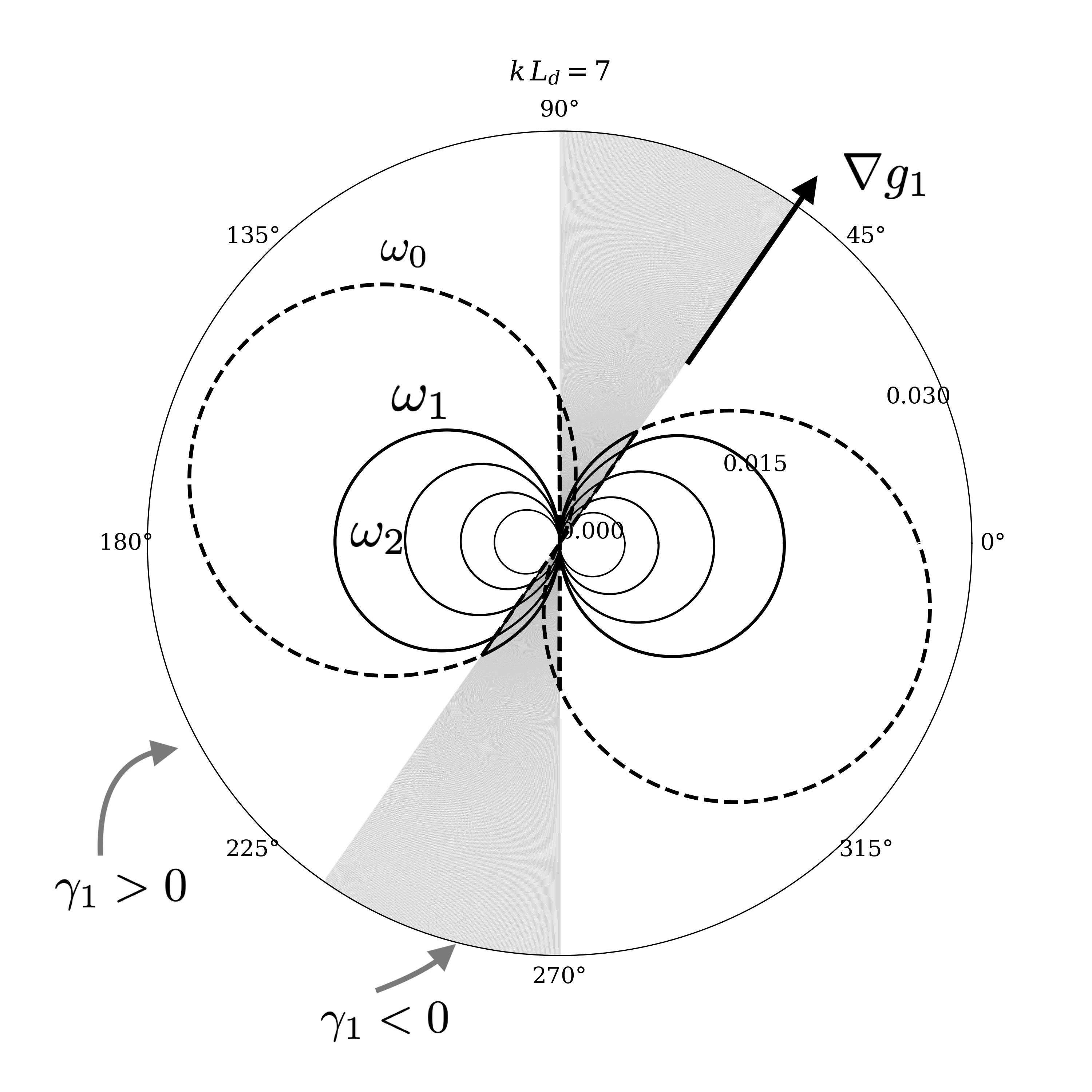
We distinguish the following cases depending on the sign of . In the following, we assume .
- i.
. All eigenvalues satisfy , all modes satisfy , and all waves propagate westward. The th mode, , has internal zeros (Binding et al. 1994). See the regions in white in figure 2.
- ii.
. There is one mode, , with a negative square, , corresponding to an eastward propagating wave. The eastward propagating wave nevertheless travels pseudowestward (to the left of the upslope direction for ). The associated eigenvalue, , satisfies . The remaining modes, for , have positive squares, , corresponding to westward propagating waves and have eigenvalues, , satisfying . Both and have no internal zeros whereas the remaining modes, , have internal zeros for (Binding et al. 1994). See the stippled regions in figures 2.
To elucidate the meaning of , note that a pure surface quasigeostrophic mode77 7 A pure surface quasigeostrophic mode is the mode found after setting with an upper boundary at . has . Thus means that the bottom-trapped mode decays away from the boundary more rapidly than a pure surface quasigeostrophic wave. Indeed, the limit of yields the bottom step-mode (37) of the previous subsection.

The step-mode limit is obtained as . This limit is found as either for propagation directions in which or as becomes parallel or anti-parallel to (whichever limit satisfies ). In this limit, we obtain a step-mode exactly confined at the boundary (that is, ) with zero phase speed [see figure 3(a)]. The remaining modes then satisfy the isentropic boundary condition
| (47) |
The other limit is that of which is obtained as the buoyancy gradient becomes large, . In this limit, the eigenvalue [see figure 3(b)]. Moreover, the phase speed of the bottom-trapped wave becomes infinite, an indication that the quasigeostrophic approximation breaks down. Indeed, the large buoyancy gradient limit corresponds to steep topographic slopes and so we obtain the topographically-trapped internal gravity wave of Rhines 1970, which has an infinite phase speed in quasigeostrophic theory. The remaining modes then satisfy the vanishing pressure boundary condition
| (48) |
as in the surface modes of de La Lama et al. 2016 and LaCasce 2017.
3.2.3 The general time-dependent solution
At some wavevector , the observed vertical structure now has the form
| (49) |
where is a twice continuously differentiable function satisfying . For such functions we can write (see appendix A)
| (50) |
so that the time-evolution is
| (51) |
Again, it is the above expression, which is valid only in linear theory with a quiescent background state, that gives the generalized Rhines modes physical meaning. Outside the linear theory of this section, the generalized Rhines modes do not have any physical interpretation and instead merely serve as a mathematical basis for .
Recall from section 33.1 that an expansion of a step-mode (37) in terms of the baroclinic modes produces a series that is identically zero. It follows that the step-modes are independent of the baroclinic modes—they constitute independent degrees of freedom. However, with the inclusion of bottom boundary dynamics, we may now expand the bottom step-mode, , in terms of the modes, , with the expansion given by
| (52) |
3.3 The generalized Rhines problem
The general problem with topography at both the upper and lower boundaries is
| (53a) | ||||
| (53b) | ||||
for , where the length-scale is given by equation (42). As the eigenvalue, , appears in both boundary conditions, the eigenvalue problem (53) takes place in . The inner product now has the form
| (54) |
which reduces to equation (44) when . Under this inner product, the eigenfunctions form a basis of .

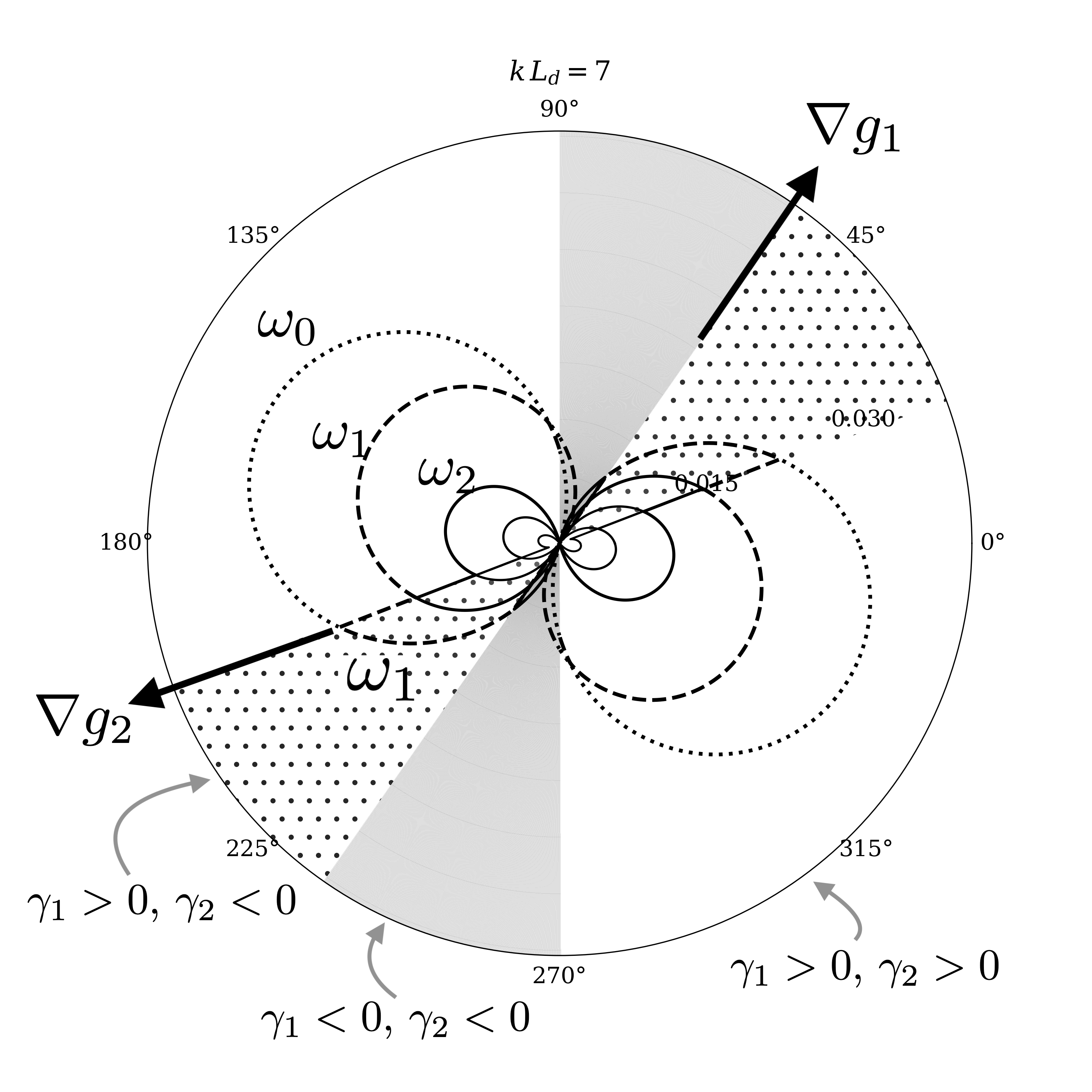
There are now three cases depending on the signs of and and as depicted in figures 4 and 5. In the following, we assume .
- i.
- ii.
- iii.
and . There are two modes and with negative squares, , that propagate eastward and have eigenvalues, , satisfying for . The remaining modes, , for have positive squares, , propagate westward, and have eigenvalues, , satisfying . The zeroth mode, , has one internal zero, the first and second modes, and , have no internal zeros, and the remaining modes, , have internal zeros for (Binding and Browne 1999). See the shaded regions in figures 2 and 4 and panels (e) and (f) in figure 5.
3.4 The vertical velocity eigenvalue problem
Let where is a non-dimensional function. For the Rossby waves with isentropic boundaries of section 33.1 (the traditional baroclinic modes), the corresponding vertical velocity modes satisfy
| (55) |
with vanishing vertical velocity boundary conditions
| (56) |
(see appendix B for details). The resulting modes form an orthonormal basis of with orthonormality given by
| (57) |
One can obtain the eigenfunctions, , by solving the eigenvalue problem (55)–(56) or by differentiating the streamfunction modes according to equation (108).
Quasigeostrophic boundary dynamics
As seen earlier, boundary buoyancy gradients activate boundary dynamics in the quasigeostrophic problem. In this case, boundary conditions for the quasigeostrophic vertical velocity problem (55) become
| (58) |
(see the appendix B). The resulting modes satisfy a peculiar orthogonality relation given by equation (114).

4 Eigenfunction expansions
Motivated by the Rossby waves of the previous section, we now investigate various sets of normal modes for quasigeostrophic theory. Let be a collection of normal modes, and assume is twice continuously differentiable in . Define the eigenfunction expansion of by
| (59) |
where
| (60) |
Because is a basis of , the eigenfunction expansion satisfies (Brown and Churchill 1993, e.g.,)
| (61) |
Significantly, the vanishing of the integral (61) does not imply because the two functions can still differ at some points .
In the following, we will only consider eigenfunctions expansions that diagonalize the energy and potential enstrophy integrals of section 22.5.
4.1 The four possible modes
There are only four bases in quasigeostrophic theory that diagonalize the energy and potential enstrophy integrals. All four sets of corresponding normal modes satisfy the differential equation
| (62) |
but differ in boundary conditions according to the following (recall that is the bottom and the surface).
- •
Baroclinic modes: Vanishing vertical velocity at both boundaries (Neumann),
(63) - •
Anti-baroclinic modes: Vanishing pressure88 8 Recall that the geostrophic streamfunction is proportional to pressure (e.g., Vallis 2017, section 5.4). at both boundaries (Dirichlet),
(64) - •
Surface modes: (mixed Neumann/Dirichlet)
(65) - •
Anti-surface modes: (mixed Neumann/Dirichlet)
(66)
All four sets of modes are missing two modes. Each boundary condition of the form
| (67) |
implies a missing step-mode while a boundary condition of the form
| (68) |
implies a missing boundary-trapped exponential mode [see the limit leading to equation (48)].
4.2 Expansions with modes
We here examine the pointwise convergence and the term-by-term differentiability of eigenfunction expansions in terms of modes. These properties of Sturm-Liouville expansions may be found in Brown and Churchill 1993 and Levitan and Sargsjan 1975.99 9 In particular, chapters 1 and 8 in Levitan and Sargsjan 1975 show that eigenfunction expansions have the same pointwise convergence and differentiability properties as the Fourier series with the analogous boundary conditions. The behaviour of Fourier series is discussed in Brown and Churchill 1993.
4.2.1 Pointwise equality on
For all four sets of modes, if is twice continuously differentiable in , we obtain pointwise equality in the interior
| (69) |
The behaviour at the boundaries depends on the boundary conditions the modes satisfy. If the satisfy the vanishing pressure boundary condition at the th boundary
| (70) |
then
| (71) |
regardless of the values of . It follows that will be continuous over and will generally have a jump discontinuity at the boundaries [unless for ]. In contrast, if the satisfy a zero vertical velocity boundary condition at the th boundary
| (72) |
then
| (73) |
Consequently, of the four sets of modes, only with the baroclinic modes do we obtain the pointwise equality on the closed interval .
However, even though converges pointwise to when the baroclinic modes are used, we are unable to represent the corresponding velocity in terms of the vertical velocity baroclinic modes since the modes vanish at both boundaries. Analogous considerations show that only the anti-baroclinic vertical velocity modes (see appendix B) can represent arbitrary vertical velocities.
4.2.2 Differentiability of the series expansion
Although we obtain pointwise equality on the whole interval with the streamfunction baroclinic modes, we have lost two degrees of freedom in the expansion process. Recall that the degrees of freedom in the quasigeostrophic phase space are determined by the potential vorticity. The volume potential vorticity, , is associated with the degrees of freedom while the surface potential vorticities, and , are associated with the degrees of freedom.
The series expansion of in terms of the baroclinic modes is differentiable in the interior . Consequently, we can differentiate the series for to recover , that is,
| (74) |
where
| (75) |
However, is not differentiable at the boundaries, , so we are unable to recover the surface potential vorticities, and . Two degrees of freedom are lost by projecting onto the baroclinic modes.1010 10 To see that is non-differentiable at , suppose that the series is differentiable and that for . But then which is a contradiction.
The energy at wavevector is indeed partitioned between the modes
| (76) |
and similarly for the potential enstrophy
| (77) |
However, as we have lost and in the projection process, the surface potential enstrophies and , defined in equation (25), are not partitioned.
4.3 Quasigeostrophic modes
Consider the eigenvalue problem
| (78a) | ||||
| (78b) | ||||
where and are non-zero real constants. This eigenvalue problem differs from the generalized Rhines eigenvalue problem (53) in that are generally not equal to the defined in equation (42). The inner product induced by the eigenvalue problem (78) is given by equation (54) with the replaced by the .
Smith and Vanneste 2012 investigate an equivalent eigenvalue problem to (78) and conclude that, when and are positive, the resulting eigenfunctions form a basis of . However, such a completeness result is insufficient for the Rossby wave problem of section 33.3, in which case and can be negative.
4.4 Expansion with modes
When in the eigenvalue problem (78) are finite and non-zero, the resulting eigenmodes form a basis for the vertical structure phase space . Thus, the projection
| (79) |
where
| (80) |
is an equivalent representation of . Not only do we have pointwise equality
| (81) |
but the series is also differentiable on the closed interval [the case of is due to Fulton 1977 whereas the case of is due to Yassin 2021.]. Thus given , we can differentiate to obtain both and and thereby recover all quasigeostrophic degrees of freedom. Indeed, we have
| (82) | ||||
| (83) |
where
| (84) | ||||
| (85) |
for .
In addition, the energy, , volume potential enstrophy, , and surface potential enstrophies, and , are partitioned (diagonalized) between the modes
| (86) | ||||
| (87) |
5 Discussion
The traditional baroclinic modes are useful since they are the vertical structures of linear Rossby waves in a resting ocean and they can be used for wave-turbulence studies such as in (Hua and Haidvogel 1986; Smith and Vallis 2001, e.g.,). Therefore, any basis we choose should not only be complete in , but should also represent the vertical structure of Rossby waves in the linear (quiescent ocean) limit. Such a basis would then amenable to wave-turbulence arguments and can permit a dynamical interpretation of field observations. The basis suggested by Smith and Vanneste 2012 does not correspond to Rossby waves in the linear limit. It is a mathematical basis with two-independent parameters that diagonalizes the energy and potential enstrophy integrals.
The Rhines modes of section 33.2 offer a basis of that corresponds to Rossby wave over topography in the linear limit. These Rhines modes do not contain any free parameters. Indeed, if we set in the eigenvalue problem (78) and let , we then obtain the Rhines modes. Note that since may be negative, the Smith and Vanneste 2012 modes do not apply. Instead, the case of negative is examined in this article and in Yassin 2021.
However, the Rhines modes, as a basis of are not a basis of the whole vertical structure phase space since they exclude surface buoyancy anomalies at the upper boundary. To solve this problem, we can use the modes of the eigenvalue problem (78) with but leaving arbitrary as in Smith and Vanneste 2012. Although this basis now only has one free parameter, , it still does not correspond to Rossby waves in the linear limit. We can even eliminate this free parameter by interpreting surface buoyancy gradients as topography e.g., by defining
| (88) |
where corresponds to the background flow, and using in place of in the generalized Rhines modes of section 33.3. However the waves resulting from topographic gradients generally differ from those resulting from vertically-sheared mean-flows (in particular, one must take into account advective continuum modes) and so this resolution is artificial.
Galerkin approximations with modes
Both the baroclinic modes and the modes have infinitely many degrees of freedom. In contrast, numerical simulations only contain a finite number of degrees of freedom. Consequently, it should be possible to use baroclinic modes to produce a Galerkin approximation to quasigeostrophic theory with non-trivial boundary dynamics. Such an approach has been proposed by Rocha et al. 2015.
Projecting onto the baroclinic modes produces a series expansion, , that is differentiable in the interior but not at the boundaries. By differentiating the series in the interior we obtain equation (75) for . If instead we integrate by parts twice and avoid differentiating , we obtain
| (89) |
The two expressions (75) and (89) are only equivalent when . For non-zero and , the singular nature of the expansion means we have a choice between equations (75) and (89).
By choosing equation (89) and avoiding the differentiation of , Rocha et al. 2015 produced a least-squares approximation to quasigeostrophic dynamics that conserves the surface potential enstrophy integrals (24). This is a conservation property underlying their approximation’s success.
6 Conclusion
In this article, we have studied all possible non-continuum collections of streamfunction normal modes that diagonalize the energy and potential enstrophy. There are four possible modes: the baroclinic modes, the anti-baroclinic modes, the surface modes, and the anti-surface modes. Additionally, we explored the properties of the family of bases introduced by Smith and Vanneste 2012 which contain two free parameters and generalized the family to allow for . This generalization is necessary for Rossby waves in the presence of bottom topography. If , where is given by equation (42) for , the resulting modes are the vertical structure of Rossby waves in a quiescent ocean with prescribed boundary buoyancy gradients (i.e., topography). We have also examined the associated and vertical velocity modes.
For the streamfunction modes, only the baroclinic modes are capable of converging pointwise to any quasigeostrophic state on the interval , whereas for the vertical velocity modes, only the anti-baroclinic modes are capable. However, in both cases, the resulting eigenfunction expansion is not differentiable at the boundaries, . Consequently, while we can recover the volume potential vorticity density, , we cannot recover the surface potential vorticity densities, and . Thus, we lose two degrees of freedom when projecting onto the baroclinic modes. In contrast, modes provide an equivalent representation of the function in question. Namely, the eigenfunction expansion is differentiable on the closed interval so that we can recover , , from the series expansion.
We have also introduced a new set of modes, the Rhines modes, that form a basis of and correspond to the vertical structures of Rossby waves over topography. A natural application of these normal modes is to the study of weakly non-linear wave-interaction theories of geostrophic turbulence found in Fu and Flierl 1980 and Smith and Vallis 2001, extending their work to include bottom topography.
Acknowledgements.
We offer sincere thanks to Stephen Garner, Robert Hallberg, Isaac Held, Sonya Legg, and Shafer Smith for comments and suggestions that greatly helped our presentation. We also thank Guillaume Lapeyre, William Young, one anonymous reviewer, and the editor (Joseph LaCasce) for their comments that helped us to further refine and focus the presentation, and to correct confusing statements. This report was prepared by Houssam Yassin under award NA18OAR4320123 from the National Oceanic and Atmospheric Administration, U.S. Department of Commerce. The statements, findings, conclusions, and recommendations are those of the authors and do not necessarily reflect the views of the National Oceanic and Atmospheric Administration, or the U.S. Department of Commerce. [A] \appendixtitleSturm-Liouville eigenvalue problems with -dependent boundary conditions Consider the differential eigenvalue problem| (90) |
in the interval with boundary conditions
| (91) |
for , where are real-valued integrable functions and are real numbers. Moreover, we assume , that and are twice continuously differentiable, that is continuous, and that .
Define the two boundary parameters for by
| (92) |
Then the natural inner product for the eigenvalue problem is given by
| (93) |
where the boundary operator is defined by
| (94) |
The eigenvalue problem takes place in the space where is the number of non-zero . Assume for the following that ; the case when is similar. If
| (95) |
for then the inner product (93) is positive definite—that is, all non-zero satisfy . Therefore , equipped with the inner product (93), is a Hilbert space. In this Hilbert space settings, the eigenfunctions form and orthonormal basis of and that the eigenvalues distinct and bounded below as in equation (43) (Evans 1970; Walter 1973; Fulton 1977). The appendix of Smith and Vanneste 2012 also proves this result in the case when . The convergence properties of normal mode expansions in this case are due to Fulton 1977.
However, as we observe in section 3, the case is not sufficient for the Rossby wave problem with topography. In general, the space with the indefinite inner product (93) is a Pontryagin space (Iohvidov and Krein 1960; Bognár 1974, see). Pontryagin spaces are analogous to Hilbert spaces except that they have a finite-dimensional subspace of elements satisfying . If is a Pontryagin space with inner product , then admits a decomposition
| (96) |
where is a Hilbert space under the inner product and is a finite-dimensional Hilbert space under the inner product . If is an orthonormal basis for the Pontryagin space , then an element can be expressed
| (97) |
Even though is normalized, the presence of in the denominator of equation (97) is essential since this term may be negative.
One can rewrite the eigenvalue problem (90)–(91) in the form for some operator (Langer and Schneider 1991, e.g.,). The operator is a positive operator if
- •
for the -dependent boundary conditions, we have
(98) - •
for the -independent boundary conditions, we have
(99)
Yassin 2021 has shown that, when is positive, the eigenfunctions of the eigenvalue problem (90)–(91) form an orthonormal basis of , that the eigenvalues are real, and that the eigenvalues are ordered as in equation (43). Moreover, since is positive, we have the relationship
| (100) |
Finally, Yassin 2021 shows that the normal mode expansion results of Fulton 1977 extend to this case as well.
[B] \appendixtitlePolarization relations and the vertical velocity eigenvalue problem
.1 Polarization relations
The linear quasigeostrophic vorticity and buoyancy equations, computed about a resting background state, are
| (101) | ||||
| (102) |
in the interior . The vorticity, , and buoyancy, , are given in terms of the geostrophic streamfunction via
| (103) | |||
| (104) |
The no-normal flow at the lower and upper boundaries implies
| (105) |
for . Substituting equation (105) into the linear buoyancy equation (102), yields the boundary conditions
| (106) |
.2 The vertical velocity eigenvalue problem
Taking the vertical derivative of (109) and using (108) yields
| (112) |
where and is non-dimensional. The boundary conditions at are
| (113) |
as obtained by using equations (109) and (108) in boundary conditions (53b). The orthonormality condition is
| (114) | ||||
where
| (115) |
When only one boundary condition is -dependent (e.g., ) the eigenvalue problem (112)–(113) satisfies equation (95) when and equations (98) and (99) when ; thus the reality of the eigenvalues and the completeness results follow. However, when both boundary conditions are -dependent the problem no longer satisfies these conditions for all . Instead, in this case, one exploits the relationship between the vertical velocity eigenvalue problem (112)–(113) and the streamfunction problem (53a)–(53b) given by equations (108) and (109) to conclude that the two problem have the identical eigenvalues (for ) and then use the simplicity of the eigenvalues to conclude that no generalized eigenfunctions can arise.
.3 The vertical velocity modes
Analogously with the streamfunction modes, we have the following sets of vertical velocity modes.
- •
Baroclinic modes: Vanishing vertical velocity at both boundaries,
(116) - •
Anti-baroclinic modes: Vanishing pressure at both boundaries,
(117) - •
Surface modes:
(118) - •
Anti-surface modes:
(119)
References
- Balmforth and Morrison (1994) Balmforth, N. J., and P. J. Morrison, 1994: Normal modes and continuous spectra. Tech. Rep. DOE/ET/53088–686, Texas University, 26 pp. https://inis.iaea.org/Search/search.aspx?orig˙q=RN:26051560.
- Balmforth and Morrison (1995) Balmforth, N. J., and P. J. Morrison, 1995: Singular eigenfunctions for shearing fluids I. Tech. Rep. DOE/ET/53088–692, Texas University, 79 pp. http://inis.iaea.org/Search/search.aspx?orig˙q=RN:26061992.
- Binding and Browne (1999) Binding, P. A., and P. J. Browne, 1999: Left definite Sturm-Liouville problems with eigenparameter dependent boundary conditions. Differential and Integral Equations, 12, 167–182.
- Binding et al. (1994) Binding, P. A., P. J. Browne, and K. Seddighi, 1994: Sturm–Liouville problems with eigenparameter dependent boundary conditions. Proc. Edinburgh Math. Soc., 37, 57–72.
- Bognár (1974) Bognár, J., 1974: Indefinite Inner Product Spaces, 223. Ergebnisse der Mathematik und ihrer Grenzgebiete. 2. Folge, Springer-Verlag.
- Brink and Pedlosky (2019) Brink, K. H., and J. Pedlosky, 2019: The Structure of Baroclinic Modes in the Presence of Baroclinic Mean Flow. J. Phys. Oceanogr., 50, 239–253, https://doi.org/10.1175/JPO-D-19-0123.1.
- Brown and Churchill (1993) Brown, J. W., and R. V. Churchill, 1993: Fourier Series and Boundary Value Problems, 348. 5th ed., International Series in Pure and Applied Mathematics, McGraw-Hill.
- Burns et al. (2020) Burns, K. J., G. M. Vasil, J. S. Oishi, D. Lecoanet, and B. P. Brown, 2020: Dedalus: A flexible framework for numerical simulations with spectral methods. Phys. Rev. Res., 2, 023068, https://doi.org/10.1103/PhysRevResearch.2.023068.
- Charney (1971) Charney, J. G., 1971: Geostrophic Turbulence. J. Atmos. Sci., 28, 1087–1095, https://doi.org/10.1175/1520-0469(1971)028¡1087:GT¿2.0.CO;2.
- Charney and Flierl (1981) Charney, J. G., and G. R. Flierl, 1981: Oceanic Analogues of Large-scale Atmospheric Motions. Evolution of Physical Oceanography, B. A. Warren, and C. Wunsch, Eds., MIT press, 448–504.
- Chelton et al. (1998) Chelton, D. B., R. A. deSzoeke, M. G. Schlax, K. El Naggar, and N. Siwertz, 1998: Geographical Variability of the First Baroclinic Rossby Radius of Deformation. J. Phys. Oceanogr., 28, 433–460, https://doi.org/10.1175/1520-0485(1998)028¡0433:GVOTFB¿2.0.CO;2.
- de La Lama et al. (2016) de La Lama, M. S., J. H. LaCasce, and H. K. Fuhr, 2016: The vertical structure of ocean eddies. Dynamics and Statistics of the Climate System, 1, dzw001, https://doi.org/10.1093/climsys/dzw001.
- Drazin et al. (1982) Drazin, P. G., D. N. Beaumont, and S. A. Coaker, 1982: On Rossby waves modified by basic shear, and barotropic instability. J. Fluid Mech., 124, 439–456, https://doi.org/10.1017/S0022112082002572.
- Evans (1970) Evans, W. D., 1970: A non-self-adjoint differentila operator in . Q. J. of Math., 21, 371–383.
- Ferrari et al. (2010) Ferrari, R., S. M. Griffies, A. J. Nurser, and G. K. Vallis, 2010: A boundary-value problem for the parameterized mesoscale eddy transport. Ocean Modelling, 32, 143–156, https://doi.org/10.1016/j.ocemod.2010.01.004.
- Ferrari and Wunsch (2010) Ferrari, R., and C. Wunsch, 2010: The distribution of eddy kinetic and potential energies in the global ocean. Tellus, 62, 92–108, https://doi.org/10.1111/j.1600-0870.2009.00432.x.
- Flierl (1978) Flierl, G. R., 1978: Models of vertical structure and the calibration of two-layer models. Dyn. Atmos. Oceans, 2, 341–381, https://doi.org/10.1016/0377-0265(78)90002-7.
- Fu and Flierl (1980) Fu, L.-L., and G. R. Flierl, 1980: Nonlinear energy and enstrophy transfers in a realistically stratified ocean. Dyn. Atmos. Oceans, 4, 219–246, https://doi.org/10.1016/0377-0265(80)90029-9.
- Fulton (1977) Fulton, C. T., 1977: Two-point boundary value problems with eigenvalue parameter contained in the boundary conditions. Proc. Royal Soc. Edinburgh Sec. A: Math., 77, 293–308.
- Held et al. (1995) Held, I. M., R. T. Pierrehumbert, S. T. Garner, and K. L. Swanson, 1995: Surface quasi-geostrophic dynamics. J. Fluid Mech., 282, 1–20, https://doi.org/10.1017/S0022112095000012.
- Hoskins et al. (1985) Hoskins, B. J., M. E. McIntyre, and A. W. Robertson, 1985: On the use and significance of isentropic potential vorticity maps. Quart. J. Roy. Meteor. Soc., 111, 877–946, https://doi.org/10.1002/qj.49711147002.
- Hua and Haidvogel (1986) Hua, B. L., and D. B. Haidvogel, 1986: Numerical Simulations of the Vertical Structure of Quasi-Geostrophic Turbulence. J. Atmos. Sci., 43, 2923–2936, https://doi.org/10.1175/1520-0469(1986)043¡2923:NSOTVS¿2.0.CO;2.
- Iohvidov and Krein (1960) Iohvidov, I. S., and M. G. Krein, 1960: Spectral theory of operators in spaces with an indefinite metric. I. Eleven Papers on Analysis, American Mathematical Society Translations: Series 2, Vol. 13, American Mathematical Society, 105–175.
- LaCasce (2017) LaCasce, J. H., 2017: The Prevalence of Oceanic Surface Modes. Geophys. Res. Lett., 44, 11,097–11,105, https://doi.org/10.1002/2017GL075430.
- Langer and Schneider (1991) Langer, H., and A. Schneider, 1991: On spectral properties of regular quasidefinite pencils . Results in Mathematics, 19, 89–109.
- Lapeyre (2009) Lapeyre, G., 2009: What Vertical Mode Does the Altimeter Reflect? On the Decomposition in Baroclinic Modes and on a Surface-Trapped Mode. J. Phys. Oceanogr., 39, 2857–2874, https://doi.org/10.1175/2009JPO3968.1.
- Lapeyre (2017) Lapeyre, G., 2017: Surface Quasi-Geostrophy. Fluids, 2, 7, https://doi.org/10.3390/fluids2010007.
- Levitan and Sargsjan (1975) Levitan, B. M., and I. S. Sargsjan, 1975: Introduction to Spectral Theory: Selfadjoint Ordinary Differential Operators, Translations of Mathematical Monographs, Vol. 39, 525. American Mathematical Society.
- Rhines (1970) Rhines, P. B., 1970: Edge-, bottom-, and Rossby waves in a rotating stratified fluid. Geophys. Astrophys. Fluid Dyn., 1, 273–302, https://doi.org/10.1080/03091927009365776.
- Rocha et al. (2015) Rocha, C. B., W. R. Young, and I. Grooms, 2015: On Galerkin Approximations of the Surface Active Quasigeostrophic Equations. J. Phys. Oceanogr., 46, 125–139, https://doi.org/10.1175/JPO-D-15-0073.1.
- Roullet et al. (2012) Roullet, G., J. C. McWilliams, X. Capet, and M. J. Molemaker, 2012: Properties of Steady Geostrophic Turbulence with Isopycnal Outcropping. J. Phys. Oceanogr., 42, 18–38, https://doi.org/10.1175/JPO-D-11-09.1.
- Schneider et al. (2003) Schneider, T., I. M. Held, and S. T. Garner, 2003: Boundary Effects in Potential Vorticity Dynamics. J. Atmos. Sci., 60, 1024–1040, https://doi.org/10.1175/1520-0469(2003)60¡1024:BEIPVD¿2.0.CO;2.
- Scott and Furnival (2012) Scott, R. B., and D. G. Furnival, 2012: Assessment of Traditional and New Eigenfunction Bases Applied to Extrapolation of Surface Geostrophic Current Time Series to Below the Surface in an Idealized Primitive Equation Simulation. J. Phys. Oceanogr., 42, 165–178, https://doi.org/10.1175/2011JPO4523.1.
- Smith and Vallis (2001) Smith, K. S., and G. K. Vallis, 2001: The Scales and Equilibration of Midocean Eddies: Freely Evolving Flow. J. Phys. Oceanogr., 31, 554–571, https://doi.org/10.1175/1520-0485(2001)031¡0554:TSAEOM¿2.0.CO;2.
- Smith and Vanneste (2012) Smith, K. S., and J. Vanneste, 2012: A Surface-Aware Projection Basis for Quasigeostrophic Flow. J. Phys. Oceanogr., 43, 548–562, https://doi.org/10.1175/JPO-D-12-0107.1.
- Straub (1994) Straub, D. N., 1994: Dispersive effects of zonally varying topography on quasigeostrophic Rossby waves. Geophys. Astrophys. Fluid Dyn., 75, 107–130, https://doi.org/10.1080/03091929408203650.
- Tulloch and Smith (2009) Tulloch, R., and K. S. Smith, 2009: Quasigeostrophic Turbulence with Explicit Surface Dynamics: Application to the Atmospheric Energy Spectrum. J. Atmos. Sci., 66, 450–467, https://doi.org/10.1175/2008JAS2653.1.
- Vallis (2017) Vallis, G. K., 2017: Atmospheric and Oceanic Fluid Dynamics: Fundamentals and Large-scale Circulation. 2nd ed., Cambridge University Press, 946 pp.
- Walter (1973) Walter, J., 1973: Regular eigenvalue problems with eigenvalue parameter in the boundary condition. Mathematische Zeitschrift, 133, 301–312.
- Wunsch (1997) Wunsch, C., 1997: The Vertical Partition of Oceanic Horizontal Kinetic Energy. J. Phys. Oceanogr., 27, 1770–1794, https://doi.org/10.1175/1520-0485(1997)027¡1770:TVPOOH¿2.0.CO;2.
- Yassin (2021) Yassin, H., 2021: Normal modes with boundary dynamics in geophysical fluids. J. Math. Phys., 62, doi:10.1063/5.0048273.