Spectral convergence of probability densities for forward problems in uncertainty quantification
Abstract.
The estimation of probability density functions (PDF) using approximate maps is a fundamental building block in computational probability. We consider forward problems in uncertainty quantification: the inputs or the parameters of a deterministic model are random with a known distribution. The scalar quantity of interest is a fixed measurable function of the parameters, and is therefore a random variable as a well. Often, the quantity of interest map is not explicitly known and difficult to compute, and so the computational problem is to design a good approximation (surrogate model) of the quantity of interest. For the goal of approximating the moments of the quantity of interest, there is a well developed body of research. One widely popular approach is generalized Polynomial Chaos (gPC) and its many variants, which approximate moments with spectral accuracy. However, it is not clear whether the quantity of interest can be approximated with spectral accuracy as well. This result does not follow directly from spectrally accurate moment estimation. In this paper, we prove convergence rates for PDFs using collocation and Galerkin gPC methods with Legendre polynomials in all dimensions. In particular, exponential convergence of the densities is guaranteed for analytic quantities of interest. In one dimension, we provide more refined results with stronger convergence rates, as well as an alternative proof strategy based on optimal-transport techniques.
Key words and phrases:
Density, Polynomial Chaos, Spectral, Uncertainty Quantification, Wasserstein, Legendre, pushforward.2010 Mathematics Subject Classification
33C47, 62G07, 65C50, 65D151. Introduction
In the modeling of physical phenomena, taking uncertainties into consideration is often done by introducing random parameters into deterministic models. If the quantity of interest (model output) is a measurable function of the inputs, then it is a random as well. In this problem, known as the forward problems in uncertainty quantification (UQ), the computational task is to compute the induced probability measure of the quantity of interest given a prescribed probability measure on the inputs and parameters. The type of relevant information varies between applications, but in many cases the full probability density function (PDF) is of interest; See e.g., [1, 10, 11, 17, 19, 27, 29, 33, 30, 42]. This paper will rigorously establish that there exist methods which approximate these PDFs with spectral accuracy.
One avenue to approximate the PDF in forward UQ problems is by nonparametric statistical approaches, e.g., a discretized cumulative distribution function, the histogram method, or kernel density estimators (KDE) [41, 48].
To obtain better accuracy, one needs to utilize the underlying structure of forward UQ problems. That is, denote the input Borel probability space by and the Borel measurable model-output map by . The measure of interest is the pushforward of by , i.e., for every Borel set . To take this structure into account, we turn to approximation-based methods (surrogate models). In this class of methods, is approximated by a simpler function for which the pushforward is easier to compute [20, 50]. For smooth quantities of interest with low- or moderate-dimensional domains, surrogate models have become the standard [20, 37], most prominently the polynomial-based methods known as generalized polynomial chaos (gPC) [21, 28, 36, 50] and their many variants, see e.g., [25, 39, 45]. The success of the gPC methods relies on their spectral convergence, when the original map is sufficiently smooth and specific domain and boundary conditions are met [51, 52]. By spectral accuracy we mean the following: let be the gPC polynomial of order (see Sec. 2). Then decays polynomially in and the order of decay improves with the order of regularity of . Crucially, the error decays exponentially in if is analytic. convergence implies convergence of the moments of to those of . Practically, this means that for analytic functions of interest , the moments converge exponentially fast in the order of approximation.
Question.
If is the gPC approximation of , does converge to with spectral accuracy?
That a sequence of functions converges to in does not guarantee that the resulting PDFs converge to in any norm, see counter-example in [15]. Despite its practical relevance, the problem of density estimation using surrogate models has so far received little theoretical treatment, see one notable example in [6]. We previously showed that convergence of to guarantees convergence of to in the Wasserstein- metric, see details in [32] and in Sec. 5. Convergence in the Wasserstein metric, however, is in general weaker than convergence of the PDFs [22, 26]. To guarantee PDF approximation, Ditkowski, Fibich, and the author [15] proved that more strict regularity conditions and convergence of to guarantee convergence of to in for all (see Theorem 4 below) and provided a spline-based method with provable convergence rates for the PDFs. Related, but not equivalent results, have also been obtained for certain monotonic triangular maps on [53], and for the approximation of stochastic PDEs [9]. From a practical standpoint, it is desirable to have a surrogate model with spectrally convergent PDFs. One would like to prove that a well-known trade-off in function approximation (e.g., in ) holds for PDF approximation as well: on the one hand, local methods (like splines) are more robust to high derivatives and non-smoothness than spectral methods (like gPC). On the other hand, local methods are usually restricted to a fixed polynomial order of convergence, whereas spectral methods converge extremely fast for smooth functions. The question of spectral PDF convergence is therefore open and interesting.
In this work, we answer the above question affirmatively for the gPC expansion with respect to Legendre polynomials. To the best of our knowledge, these are the first results of this kind. Under high regularity conditions, the PDFs obtained by the gPC method converge spectrally (Theorem 1), and in particular converge exponentially fast for analytic quantities of interest. In the one-dimensional case we prove a stronger result, that (Theorem 2), and provide an alternative spectral convergence result (Theorem 5), for which the proof relies on the weak Wasserstein- convergence combined with a recent result by Chae and Walker [7]. In all these results, the analysis relies on three main analytic components - the relation between and (5), the approximation power of gPC in Sobolev spaces (4), and Sobolev-Morrey embeddings in compact domains (10). In this work, we study pushforward measures induced by full-grid (or tensor-product grid) polynomial approximations. In high dimensions, the use of tensor-product grids becomes computationally expansive due to the so-called curse of dimensionality - the computational cost required to achieve a certain accuracy increases exponentially with the dimension. Several approaches have been developed to perform high-dimensional uncertainty propagation, such as sparse grids [3, 5, 50, 51] and adaptive methods [45]. While these methods are beyond the scope is of this work, our analysis lays the numerical analysis foundation to understand the pushforward measures they induce, and thus their adequacy for density estimation.
1.1. Paper structure
The remainder of the paper is organized as follows: Sec. 2 provides the preliminaries on the gPC method, pushforward measures and a more detailed account of previous results. Secs. 3 and 4 detail the paper’s main theoretical results and their proofs, respectively. We then turn in Sec. 5 to provide an alternative, optimal-transport based analysis of the measure pushforward problem. Finally, in Sec. 6 we present numerical experiments and outline open problems.
2. Preliminaries
2.1. Generalized Polynomial Chaos
We present a brief review of the gPC method, see [50] for a thorough introduction. For clarity, we first review the gPC method for the one-dimensional case. The Legendre polynomials are the set of orthogonal polynomials with respect to the Lebesgue measure on , see [38]
The Legendre polynomials constitute an orthonormal basis of , i.e.,
| (1) |
The Galerkin-gPC expansion of a function of order is the projection of to its first modes, i.e., . In the multidimensional case , the expansion of order of is defined as the projection of into the space of polynomials of maximal degree [8, 21, 52]
| (2) |
where is the tensor-product Legendre polynomial of multi-index and . If can only be evaluated at a discrete set of points, the integrals in expansion coefficients cannot be exactly computed. The collocation-gPC approach is to approximate these coefficients using the Gauss quadrature formula: Let be an integrable function, then the Gauss-Legendre quadrature formula of order is , where are the distinct and real roots of , are the weights, and are the Lagrange interpolation polynomials with respect at the quadrature points [14]. Taking yields the gPC collocation method in one dimension [51],
| (3a) | |||
| (3b) |
The generalization of (3) to multiple dimensions is a direct result of integration by tensor-grid Gauss quadratures, see [8, 14, 51] for details. We further note that the gPC-collocation polynomial (3) is also the polynomial interpolant of degree in the Guass-Legendre points, i.e., for all quadrature points [12].
2.2. The approximation power of Legendre polynomials
Recall that for or , and any pair of integers , the corresponding Sobolev space is defined as [2, 18]
where is a multi-index and . For we will adopt the conventional notation . Both the Galerkin (2) and the collocation expansion (3) converge spectrally in , where the underlying measure is the Lebsegue measure [24, 40, 47, 50]. By this we mean that if for some , then [8, 24, 50]
and if is analytic (in the multivariate sense), then decays exponentially in [13], See [53] and the references therein for details. From a probability and UQ point of view, the convergence in guarantees that the moments of converge to the moments of . Indeed, if is the Lebesgue measure on , a simple application of the Cauchy-Schwartz inequality shows that
and therefore for e.g., a smooth quantity of interest , the gPC method provides an accurate approximation of for a relatively low order . The convergence of other moments follow similarly, see e.g., [15].11 1 For measures which are not the Lebesgue measure, see [16]. Both gPC expansions (2) and (3) also converge in higher-regularity Sobolev spaces, as given by the now classical result:
Theorem (Canuto and Quarteroni [8]).
If is analytic (for ) on an ellipse in with foci at and with both axis summing to , then in one dimension [46, 47]. By Parseval identity (with respect to Legendre polynomials),
and so the approximation error is almost exponential as well. Furthermore, by uniform convergence of to on , one can differentiate term-wise, yielding faster than polynomial (exponential for all practical purposes) convergence of to in all Sobolev spaces with .
2.3. Pushforward measures and prior results
The pushforward of a Borel measure on by a measurable is a measure defined by for any Borel subset . If a measure on is absolutely continuous with respect to the Lebesgue measure, its probability density function (PDF) is its Radon-Nykodim derivative, i.e., which satisfies for any Borel set . Alternatively, if the cumulative distribution function (CDF) is differentiable, then . In the one-dimensional case, if is piecewise and piecewise monotonic, and is an absolutely continuous probability measure, then [15]
| (5) |
This relation is the source of many of the difficulties and peculiarities in understanding PDFs of pushforward measures. For example, if for some constant on an interval with , then has a singular part at and therefore has no PDF. Even for a non-constant smooth monotonic function such as and a simple such as the uniform measure on , then is singular. Analogously for , then , where is the -dimensional surface elements.
The practical goal of surrogate models in the context of PDF approximation is to approximate by with small error terms for some , while maintaining small, as is a good proxy to the computational cost. To see that, first note that since sampling arbitrarily many times from the polynomial is computationally cheap, approximating to arbitrary precision given is relatively cheap as well, see the analysis in [15]. Therefore, it is constructing which is costly. In the collocation gPC (3), the larger the degree of approximation is, the more evaluations of are required. If for example models the response of a partial differential equation (PDE), each such evaluation amounts to a solution of the PDE, which is usually computationally expansive. In the Galerkin-type gPC (2), one usually projects the original PDE with random parameters to several PDEs with deterministic parameters, the number of which also grows with the degree , see [50] for details. Therefore, in either case guaranteeing good accuracy for a small degree should be the goal of our analysis.
As noted in the introduction, convergence alone does not guarantee convergence of the pushforward PDFs. Indeed, one can construct a sequence such that in but for all [15]. Previously however [32], we proved that convergence is sufficient to establish convergence in the weaker Wasserstein metric, or more precisely, that (see relevant definitions in Sec. 5). Furthermore, we showed that uniform boundedness of combined with convergence guarantees Wasserstein- convergence for any , see (26) below. Since is equal to the convergence of the CDFs [34, 43], the convergence of the CDFs in is a corollary of our result. A result in the direction of PDF approximation by surrogate methods was obtain by Ditkowski, Fibich, and the author in [15]. If is taken to be the spline interpolant of of order , on e.g., a uniform grid with a total of grid points, then for any . The main characteristic of splines that is useful to establish this result is the pointwise convergence of to , see Theorem 4 below. We will use this tool tool later to prove Theorem 1.
2.4. Problem formulation
Let be equipped with an absolutely continuous probability measure . Consider a smooth function of interest and let be its generalized polynomial chaos (gPC) approximation - either its projection to the space of Legendre polynomials of order (Galerkin type) or its polynomial interpolant on the Gauss-Legendre quadrature points of order (collocation type). Consider the pushforward measures and and denote their respective probability density functions (PDF) by and . In what follows, we see under what conditions converges to in for , and find the convergence rates.
3. Main results
The convergence of the pushed-forward PDFs is guaranteed by the following:
Theorem 1.
Let for any , let where
| (6) |
let with , and assume that . Then for any ,
For the one-dimensional case, the result can be improved:
Theorem 2.
Let , let with and let with . If for finitely many points and there exist for each such that , then
| (7) |
where . In particular, if for all , then
| (8) |
Furthermore, if is analytic on an ellipse in with foci at and with both radius summing to , converges faster than any polynomial in .
Theorem 2 improves Theorem 1 in the case of in two ways - First, it allows for points with . Second, Theorem 2 improves the convergence rate by three orders, from to . Generally, Theorem 2 also yields much smaller constants. These improvements are owed to our ability to link the PDF convergence directly to convergence of to . Since the PDFs depend on , it is conjectured that convergence of to in is the weakest convergence that guarantees convergence of the PDFs, thus possibly leading to a sharp rate in (8). In Theorem 1, we use convergence of to , which by Sobolev embedding depends on the much stronger, and therefore much slower, convergence. The improvement of rates also implies the improvement of constants, as can be observed from the Canuto and Quarteroni result (4). Suppose one wishes to guarantee , and that . Since Theorem 2 uses convergence, the constant would increase with , whereas in Theorem 1 it would depend on .
That the convergence constants depend on high-regularity Sobolev norm is emblematic of global methods in general, and spectral methods in particular: To approximate a function with high derivatives well, i.e., in the asymptotically guaranteed rate, one has to to use a gPC polynomial of a relatively high order. This high threshold resolution is often embodied in the constants of the upper bound. Here one draws a distinction between the spline-based surrogate proposed in [15] and the spectral methods: splines guarantee polynomial convergence with low-sensitivity to high-derivatives. Global polynomial methods, such as gPC, can provide exponential accuracy if is very smooth in comparison to the sampling resolution. Another way in which even Theorem 2 depends on high-order Sobolev norms, is that it requires that is at least in . This is a technical requirement that is needed to guarantee that does not grow with , see Lemma 3. Simulations seem to suggest that this is not a sharp requirement, see Sec. 6.
4. Proofs of main results
Throughout this paper we need to establish the approximation of by , and that is uniformly bounded in .
Lemma 3.
Under the conditions of Theorem 1, is uniformly bounded for all , and
| (9) |
Proof.
Recall the Sobolev-Morrey embedding theorem [2, 18]: If , and , then
| (10) |
where is the lower integer value for any .22 2 In this study, we will not use a stronger version of these embeddings for Hölder norms , but just the integer-power norms. By (10), choosing yields
| (11) |
Applying the Sobolev approximation result (4) to (11) yields
| (12) |
To guarantee a uniform bound for all , it is sufficient to choose such that . Since , then
For , then in (12), and so . Hence, since , then
We proceed to prove the estimate (9). By Sobolev-Morrey inequality (10) and (4), we have that
where
which is positive for all . ∎
4.1. Proof of Theorem 1
Local convergence as established in Lemma 3 implies convergence of PDFs by the following result:
Theorem 4 (Corollary 5.5, [15]).
Let , and consider such that . Then if
| (13a) | |||
| for some constant and for all , and if | |||
| (13b) | |||
then for all but points, and therefore
for all . Furthermore, if and interpolates at the endpoints , then the uniform estimate holds.
4.2. Proof of Theorem 2
For brevity, we omit the subscripts, denoting and . First, we treat the case where . Suppose is monotonic increasing, i.e., . By the embedding theorem (10), that implies that and so
| (14) |
for every [15, Lemma 4.1]. Since is a polynomial, . Furthermore, by Lemma 3 we have that , and so for sufficiently large , for all . Therefore for every . It might be that the ranges of and , which are the supports of and , respectively, do not overlap. Assume for simplicity that but , the other cases can be treated similarly. Then
| (15) |
We begin with the second integral -
where the last inequality is due to the Sobolev-Morrey embedding (10). Therefore, we need only to consider the first integral in (15), and we therefore assume without loss of generality that , and so
| (16) |
Denote and , then by change of variables
Since and are differentiable, then for any
| (17) | ||||
| (18) | ||||
| (19) |
where . In general, as depends on , and might not be bounded. However, as in Lemma 3, and therefore are uniformly bounded for all . Since for sufficiently large , then substituting (17) in the integral yields
| (20) |
Since , then by the Cauchy-Schwartz inequality is bounded from above by
To bound in (20) from above, we first note that by Lagrange’s mean-value theorem, there exists between and such that , and therefore . From here, the process of bounding from above is the same as bounding , which yields . Therefore . Applying the relevant Sobolev approximation theorem (4), settles the case where .
We now turn to the case where and vanish at finitely many points. As we show, it does not matter whether these zero points coincide or not, and we will therefore treat the case where , and for all . Assume without loss of generality that .33 3 We showed how to treat the case where the ranges of and do not overlap above. Fix and divide the integral for on the left hand side of (16) into two domains - (1) isolating the singular point in the PDF, i.e., and (2) the rest of the domain, .
- (1)
On the first domain , we take a crude estimation
(21a) Taking, for example , by a change of variables we get (21b) - (2)
The integral on reads the same as (20), where is replaced by , yielding
(22) where is -independent. How does depend on ? Since in the worst case but , then by Taylor expansion, for sufficiently small .
By combining both upper bounds, we have that
This upper bound is minimized by equating its derivative to zero, which yields . Hence, for sufficiently small (i.e., for sufficiently large ), .
Finally, we reduce the general case where has finitely many nodal points . In the integral , we take out the intervals and treat them separately, as in (21). For value outside these intervals, we claim that and have the same sign, for sufficiently large . We split the discussion into two cases. First, if changes its sign at , then there are two points in the interval where is maximized and minimized. Taking to be sufficiently large, then has to be positive and negative at these points, respectively, due to the pointwise approximation (9). Therefore, must change its sign in between. It might be that changes its sign within this interval again, but outside of this interval, since , then has the same sign as there for sufficiently large . The second case is easier - if does not change its sign at , then outside the interval , and so by (9) .
5. A transport-based convergence result for
In this section, we present a different convergence result for the one-dimensional collocation gPC. This method of proof highlights the role that the “weaker” Wasserstein metric can play in understanding PDFs, and the potential such methods have for future works. The result only applied to the Gauss-Lobatto (GL), defined as the roots of , the derivative of the Legendre polynomial of order , plus the endpoints . The polynomial interpolant at GL quadrature points admits the same Sobolev approximation theory as stated in (4) for the Gauss-Legendre points, see [8] and [31, Chapter 10]. As we will see, the following result is restricted to the GL interpolant since the condition guarantees that .
Theorem 5.
Let . For any integer , and any function with and , let be its polynomial interpolant at the GL quadrature points of order , and suppose the where . Then
| (23) |
where .
For analytic functions, both Theorems 2 and 5 guarantee faster than polynomial convergence. For functions , however, Theorem 2 guarantees slightly better convergence rates. Theorem 5 does improve on Theorem 2 in that it relaxes the demand to . But as noted, the importance of Theorem 5 is the method of its proof, which relies on the Wasserstein distance.
Given two probability measures and on , the Wasserstein- distance is defined as44 4 To avoid confusion - denotes the Sobolev spaces of functions with derivatives which are integrable, and denotes the Wasserstein- distance (instead of the standard ).
| (24a) | |||
| where is the set of all measures on for which and are marginals, i.e., for any Borel , | |||
| (24b) | |||
Since , a minimizer of (24) exists, and so is finite, and it is a metric [35, 44]. Intuitively, the Wasserstein distance is often referred to as the earth-mover’s distance; computes the minimal work (distance times force) by which one can transfer a mound of earth in the mold of to a one that is in the mold of .
How does the Wasserstein distance relate to the problem of densities? In general, , but not the other way around [22]. This is why, in general, the Wasserstein distance induces a weaker topology on the space of probability measures than that induced by the distance between the PDFs. Moreover, the Wasserstein distance is even well-defined for singular measures, which do not have densities at all. A recent result due to Chae and Walker, however, shows that if the densities are sufficiently regular, the Wasserstein- metric bounds from above the distance between the densities.
Theorem (Chae and Walker [7]).
Let and be two Borel measures on with PDFs for some . Then
| (25) |
As we will show in Lemma 6, one can verify under what conditions and are sufficiently regular. Therefore, to prove convergence of to , it is sufficient to prove the convergence of . The weak convergence in the Wasserstein metric has recently been established under much more general conditions by the author:
Theorem ([32]).
For any compact Borel set , and for every ,
| (26) |
where the implicit constant depends only on , , and .
Proof of Theorem 5.
To apply (25) to and , we need to show that their densities are sufficiently regular.
Lemma 6.
Let and let with for all , and denote . Then , for sufficiently large , and
where the implicit constant does not depend on .
proof of lemma.
We begin, for simplicity, with . By (5), if is monotonic, formally,
| (27) |
By Sobolev-Morrey embedding (10), . Combined with the fact that , then . For , due to Lemma 3, on for all sufficiently large , and is also uniformly bounded for all ( is a polynomial, and therefore smooth). By the analog of (27) for and , we have that . Since is uniformly bounded in terms of and its derivatives, for all sufficiently large . Here it is key that our domain is one-dimensional, that interpolates at the endpoints , and that both functions are monotonic. These three facts ensure that
Suppose otherwise that, without loss of generality, . In this case would generically have a step-like discontinuity at , and therefore .
For a general , by direct differentiation one has that is a sum of rational functions where the numerators depend on and in , and the denominators are monomials in . One then generalizes Lemma 3 to show that adequately-high derivatives of are uniformly bounded in , which concludes the Lemma. ∎
Lemma 6 implies that (25) is applicable in our settings, and that , where the upper bound depends only on and its derivatives. Therefore
| (28) |
Since is compact, (26) can be applied to such that (28) yields
| (29) |
By the spectral convergence, , see (4). To bound the error, we use (10) in conjuction with (4) again, yielding . Applying both of these upper bounds to (29) than yields
∎
The following heuristic argument suggests that the condition is necessary for the proof of Theorem 5. Let be the uniform density, and suppose without loss of generality that is monotonic increasing, that , and that by Taylor expansion for some integer and as . Then and by direct substitution into (27)
which is not integrable in any neighborhood of . Hence, for any , and we cannot use (25).
6. Numerical experiments and open questions
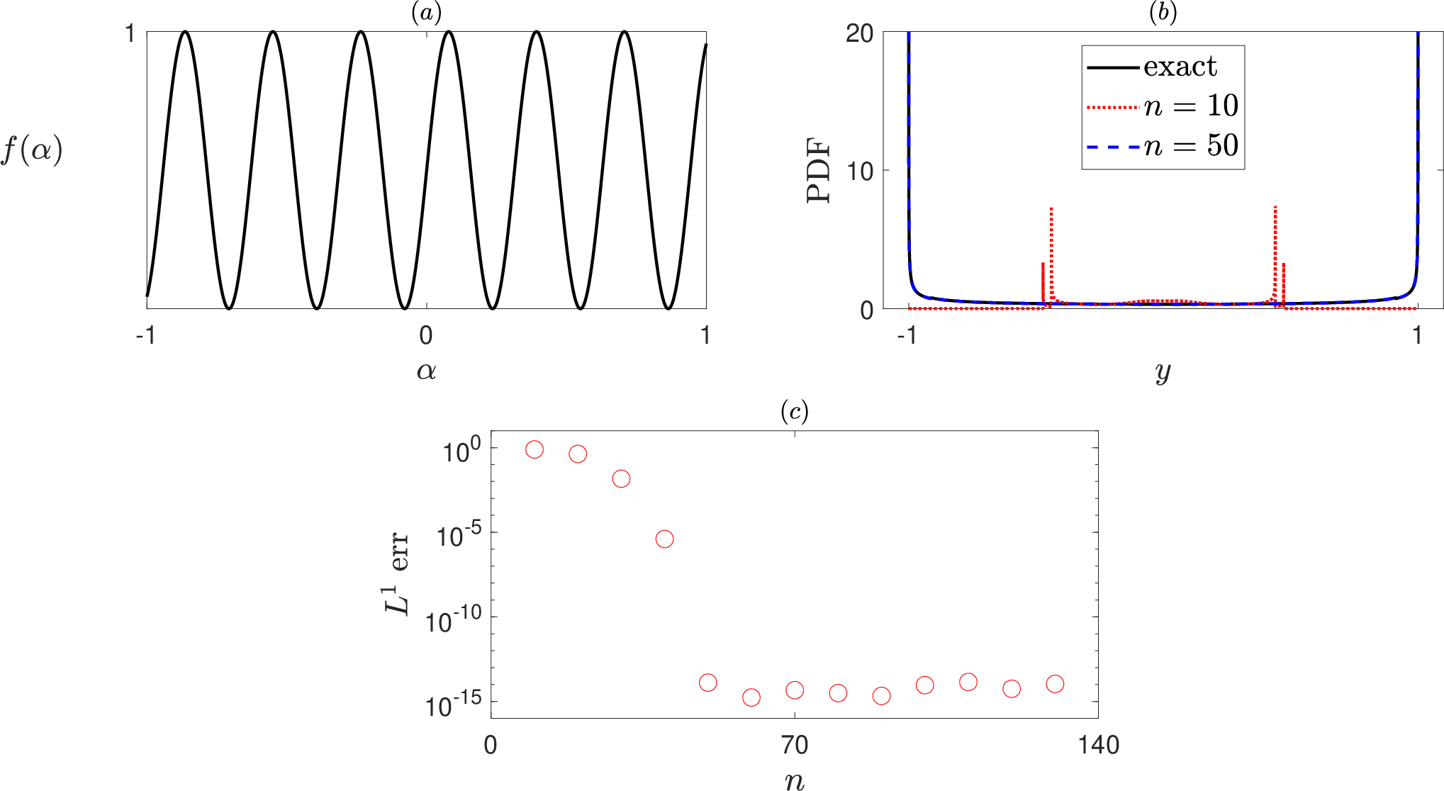
We highlight some aspects of density-approximation using the gPC collocation method (3) by numerical experiments on where is the uniform probability measure on . We first consider , see Fig. 1(a). The approximation in and of by polynomials is quite standard: a small number of collocation points (conversely, a low-order polynomial) does not suffice to resolve the oscillations of . Once is sufficiently large, since is analytic, we expect to converge to in exponentially fast, for every . For the PDF, we see that indeed approximates quite poorly, whereas is nearly indistinguishable from ; see Fig. 1(b). Quantitatively, the error between the PDFs follows the expected pattern - no convergence for , but then a sharp, exponential decay until machine-precision is reached; see Fig. 1(c). Another interesting facet of this example is that since at several points, is singular at , see (5). Theorem 2 therefore implies that since at the maximas and minimas, see (7). However, since decays exponentially with , the effect of this loss of accuracy is hardly noticeable.

We repeat the same experiment in higher dimension, using the gPC interpolant on the Gauss-Legendre tensor-product quadrature points (using the Sparse Grid Matlab Kit [3]). First, for , we test , for which we get similar behavior as we got for ; compare Fig. 1(c) with Fig. 2(a). Next, to observe “simpler” exponential convergence, we test in the functions and , in Figs. 2(b) and 2(c), respectively. Note that in all three figures the error convergence is plotted against , the maximal polynomial degree, see e.g., (2). The computational cost, however, as represented by the number of grid point, hence the number of evaluations of , scales is .

Our next two examples are of non-smooth functions. It is generally not advisable to approximate such functions with global polynomial methods such as gPC, and we do not promote this as a strategy in this work. Rather, we consider non-smooth functions to examine the sharpness and scope of our theory. In Fig. 3 we consider . This is case not covered by Theorem 2, as but not in . Notwithstanding, we observe numerically that , which is comparable to which by (4) converges as . Recall that the requirement in Theorem 2 that stems from our use of Sobolev embedding in Lemma 3 to guarantee that is uniformly bounded in . This boundedness is numerically satisfied in this example (results not shown), even though it is not guaranteed by our current theory.
Numerically, it seems that the -dependence of the upper bound (7) might not be tight. Since , by applying (7) with we expect that , which is much slower then what we observe in practice. Finally, consider a third function, , which is in but not in , see Fig. 4. While it is certainly not good practice to approximate such non-smooth functions with global polynomials, it is interesting to see that even so, . In comparison, since , the theoretically-predicted convergence rate of to by (4) is slower than , but was computed to be roughly (results not shown). That convergence is obtained implies that stronger mechanisms of PDF convergence at at play than what our current theory accounts for.

This work also lays the foundations to the study of pushforwards by sparse-grid representations, which are of great practical importance. A key impediment to approximation in the multidimensional case is the so-called curse of dimensionality - the computational cost of constructing grows exponentially with the dimension . For example, the collocation gPC on a tensor-grid of quadrature-points requires sampling at points, which becomes non-feasible already for relatively moderate dimensions. A common approach to this problem in approximation (which in the UQ context is equivalent to the approximation of moments) is by using sparse grid, which allow for superior orders of convergence [3, 5, 50, 51]. Applying our current analytic approach to sparse grids would require a detailed analysis of the convergence of sparse quadratures in high-order Sobolev spaces.55 5 Not to be confused with the more standard topic of or convergence sparse-representations of high-regularity functions for . To the best of our knowledge, there are few relevant results in this direction, see [23] and the references therein. However, as Theorem 2 suggests for , it might be that a sharper result is possible in as well. Such improvements of Theorem 1 might relax the dependence in high-order Sobolev norms to convergence, a widely studied and well understood topic [4, 5].
7. Acknowledgments
The author would like to thank A. Ditkowski, G. Fibich, S. Steinerberger, L. Tamellini, H. Wang, and M.I. Weinstein for useful comments and discussions. The author acknowledges the support of the AMS-Simons Travel Grant.
References
- [1] M.J. Ablowitz and T.P. Horikis. Interacting nonlinear wave envelopes and rogue wave formation in deep water, Phys. Fluids, 27 (2015), pp. 012107.
- [2] RA Adams and JJ Fournier, Sobolev Spaces, Elsevier, 2003.
- [3] J Bäck, F Nobile, L Tamellini, and R Tempone. Stochastic spectral Galerkin and collocation methods for PDEs with random coefficients: a numerical comparison. In J.S. Hesthaven and E.M. Ronquist, editors, Spectral and High Order Methods for Partial Differential Equations, volume 76 of Lecture Notes in Computational Science and Engineering, pages 43–62. Springer, 2011.
- [4] V Berthelmann, E Novak, and K Ritter, High dimensional polynomial interpolation on sparse grids, Adv. Comput. Math., 12, 1999, pp. 273–288.
- [5] HJ Bungartz and M Griebel, Sparse grids, Acta Numerica, 13, 2004, pp. 147–269.
- [6] T Butler, J Jakeman, and T Widely, Convergence of probability densities using approximate models for forward and inverse problems in uncertainty quantification, SIAM J. Sci. Comput., 40, 2018, A3523–A3548.
- [7] Chae M and Walker SG, Wasserstein upper bounds of the total variation for smooth densities, Stats. Probab. Lett., 163 (2020), pp. 108771.
- [8] C Canuto and A Quanteroni, Approximation results for orthogonal polynomials in Sobolev spaces, Math. Comput., 38 (1982), pp. 67–86.
- [9] G Capodaglio, M Gunzburger, and HP Wynn, Approximation of probability density functions for SPDEs using truncated series expansions, arXiv preprint arXiv:1810.01028, 2018.
- [10] Q.Y Chen, D. Gottlieb, and J.S. Hesthaven. Uncertainty analysis for the steady-state flows in a dual throat nozzle, J. Comput. Phys., 204 (2005), pp. 378–398.
- [11] I. Colombo, F. Nobile, G. Porta, A. Scotti, and L. Tamellini. Uncertainty quantification of geochemical and mechanical compaction in layered sedimentary basins, Comput. Methods Appl. Mech. Engrg., 328 (2018), pp. 122–146.
- [12] PG Constantine, MS Eldred, and ET Phipps, Sparse pseudospectral approximation method, Comput. Methods Appl. Mech. Engrg., 229 (2012), pp. 1–12.
- [13] PJ Davis, Interpolation and Approximation, Dover, 1975.
- [14] PJ Davis and P Rabinowitz, Numerical Integration, Academic, New York, 1975.
- [15] A Ditkowski, G Fibich, and A Sagiv, Density estimation in uncertainty propagation problems using a surrogate model, SIAM/ASA J. Uncertain. Quantif., 8 (2020), pp. 261-300.
- [16] A Ditkowski and R Katz, On spectral approximations with nonstandard weight functions and their implementations to generalized chaos expansions, J. Sci. Comput., 79 (2019), pp. 1985–2005.
- [17] D Estep, A Malqvist, and S Tavener, Nonparametric density estimation for randomly perturbed elliptic problems I: computational methods, a posteriori analysis, and adaptive error control, SIAM J. Sci. Comput., 31, 2009, pp. 2935–2959.
- [18] LC Evans, Partial Differential Equations, (Vol. 19) American Mathematical Society, 2010.
- [19] B. Ganapathysubramanian and N. Zabaras. Sparse grid collocation schemes for stochastic natural convection problems, J. Comp. Phys., 225 (2007), pp. 652–685.
- [20] R. Ghanem, D. Higdon, and H. Owhadi. Handbook of Uncertainty Quantification, Springer, New York, 2017.
- [21] R. Ghanem and P.D. Spanos. Stochastic Finite Elements: a Spectral Approach, Springer-Verlag, New-York, 1991.
- [22] A.L. Gibbs and F.E. Su, On choosing and bounding probability metrics, Int. Stats. Rev., 70:419–435, 2002.
- [23] M Griebel and S Knapek, Optimized general sparse grid approximation spaces for operator equations, Math. Comput., 78, 2009, pp. 2223–2257.
- [24] J.S. Hesthaven, S. Gottlieb, and D. Gottlieb. Spectral Methods for Time-Dependent Problem, Cambridge, UK, 2007.
- [25] O.P. Le Maître, O.M. Knio, H.N. Najm, and R. Ghanem. Uncertainty propagation using Wiener–Haar expansions, J. Comp. Phys., 197 (2004), pp. 28–57.
- [26] L. Le Cam and G.L. Yang. Asymptotics in Statistics: Some Basic Concepts, Springer Science & Business Media, New York, 2012.
- [27] O.P. Le Maître, L. Mathelin, O.M. Knio, and M.Y. Hussaini. Asynchronous time integration for polynomial chaos expansion of uncertain periodic dynamics, Discrete Contin. Dyn. Syst, 28 (2010), pp. 199–226.
- [28] A. O’Hagan. Polynomial chaos: A tutorial and critique from a statistician’s perspective. SIAM/ASA J. Uncertain. Quantif., 20 (2013), pp. 1–20.
- [29] G. Patwardhan, X. Gao, A. Sagiv, A. Dutt, J. Ginsberg, A. Ditkowski, G. Fibich, and A.L. Gaeta. Loss of polarization of elliptically polarized collapsing beams. Phys. Rev. A, 99 (2019), pp. 033824.
- [30] Piazzola C, Tamellini L, Pellegrini R, Broglia R, Serani A, and Diez M, Uncertainty quantification of ship resistance via multi-index stochastic collocation and radial basis function surrogates: a comparison, AIAA Aviation 2020 Forum, pp. 3160, 2020.
- [31] A Quarteroni, R Sacco, and F Salero, Numerical Mathematics, Springer-Verlag, New York NY, USA, 2000.
- [32] A Sagiv, The Wasserstein distances between pushed-forward measures with applications to uncertainty quantification, arXiv preprints, arXiv:1902.05451 (to appear in Comm. Math. Sci.)
- [33] A Sagiv, A Ditkowski, and G Fibich, Loss of phase and universality of stochastic interactions between laser beams, Opt. Exp., 25 (2017), pp. 24387–24399.
- [34] T. Salvemini, Sul calcolo degli indici di concordanza tra due caratteri quantitativi, Atti della I Riunione della Soc. Ital. di Statistica, Roma, 1943.
- [35] F Santambrogio, Optimal Transport for Applied Mathematicians. Calculus of Variations, PDEs, and Modeling, Progress in Nonlinear Differential Equations and their Applications, Birkäuser, New York, 2015.
- [36] G. Stefanou. The stochastic finite element method: past, present and future, Comput. Methods Appl. Mech. Engrg., 198 (2009), pp. 1031–1051.
- [37] B. Sudret and A. Der Kiureghian. Stochastic Finite Element Methods and Reliability: a State-of-the-Art Report, Department of Civil and Environmental Engineering, University of California Berkeley, Berkeley, CA, 2000.
- [38] G. Szego. Orthogonal Polynomials, Amer. Math. Soc. Colloq. Publ., 23, American Mathematical Society, New York, 1939.
- [39] R Tipireddy and R Ghanem, Basis adaptation in homogeneous chaos spaces, J. Comput. Phys., 259, 2014, pp. 304–317.
- [40] L.N. Trefethen. Approximation Theory and Approximation Practice, SIAM, Philadelphia, PA, 2013.
- [41] A.B. Tsybakov. Introduction to Nonparametric Estimation, Springer, New York, 2009.
- [42] S. Ullmann and J. Lang. POD-Galerkin modeling and sparse-grid collocation for a natural convection problem with stochastic boundary conditions, in Sparse Grids and Applications, Munich, Spring (2012), pp. 295–315.
- [43] S.S. Vallender, Calculation of the Wassertein distance between probability distributions on the line, SIAM Theory Prob. Appl., 18:784–786, 1974.
- [44] C Villani, Topics in Optimal Transportation, American Mathematical Society, 2003.
- [45] X Wan and GE Karniadakis, An adaptive multi-element generalized polynomial chaos method for stochastic differential equations, J. Comput. Phys., 209 (2005), pp. 617–642.
- [46] H Wang, How fast does the best polynomial approximation converge than Legendre projection? Numer. Math., 147 (2021), pp. 481–583.
- [47] H. Wang and S. Xiang, On the convergence rates of Legendre approximation, Math. Comp., 81 (2012), pp. 861–877.
- [48] L Wasserman, All of Nonparametric Statistics, Springer Science & Business Media, 2006.
- [49] L Wasserman, All of Statistics: A Concise Course in Statistical Inference, Springer Science & Business Media, New York, 2004.
- [50] D. Xiu. Numerical Methods for Stochastic Computations: a Spectral Method Approach. Princeton University, Princeton, NJ, 2010.
- [51] D. Xiu and J.S. Hesthaven. High-order collocation methods for differential equations with random inputs. SIAM J. Sci. Comput., 27 (2005), pp. 1118–1139.
- [52] D. Xiu and G.E. Karniadakis. The Wiener–Askey polynomial chaos for stochastic differential equations, SIAM J. Sci. Comput., 24 (2002), pp. 619–644.
- [53] J Zech and Y. Marzouk, Sparse approximation of triangular transports on bounded domains, arXiv preprint arXiv:2006.06994, 2020.