Uplink Beam Management for Millimeter Wave Cellular MIMO Systems with Hybrid Beamforming

We consider a mmWave point-to-point communication system comprising one User Equipment (UE) having $N_{\rm ue}$ antennas and a Base Station (BS) equipped with $N_{\rm bs}$ antennas. The antenna elements at the UE are assumed to form a linear array, while the antenna elements at the BS are placed on planar panels. More specifically, the coplanar BS antennas are grouped into $M_{\rm bs}\ll N_{\rm bs}$ planar antenna packages, termed hereinafter as Antennas in Packages (AiPs) [26]. Each of these AiPs is comprised of one $N_{\rm bs,h}\times N_{\rm bs,v}$ planar array, where $N_{\rm bs,h}$ and $N_{\rm bs,v}$ denote the number of antenna elements in the horizontal and vertical directions, respectively; it clearly holds that $M_{\rm bs}N_{\rm bs,h}N_{\rm bs,v}=N_{\rm bs}$. The number of RF chains at the UE is assumed to be $N_{\rm ue}$ with each UE antenna connected to a distinct RF chain, and each AiP at the BS side is considered connected to a dedicated RF chain. Hence, $M_{\rm bs}$ RF chains in total are available at the BS, which possesses HBF capability, while the UE performs fully digital BF.

Among the available HBF architectures [8], belongs to the AiP-based (or partially connected) architecture, according to which the analog beamformer has a specific block diagonal structure. In this paper, we focus on UL communication and assume that the BS employs the following $N_{\rm bs}\times M_{\rm bs}$ analog combiner:

where the complex-valued $N_{\rm bs,h}N_{\rm bs,v}$-element column vector $\mathbf{u}_{i}$ with $i=1,2,\dots,M_{\rm bs}$ represents the BF vector at the BS’s $i$-th AiP, whose elements are assumed to have unit magnitude, i.e., $|[\mathbf{u}_{i}]_{n}|^{2}=1$ $\forall$$n=1,2,\ldots,N_{\rm bs,h}N_{\rm bs,v}$. In addition, we assume that $\mathbf{u}_{i}\in\mathbb{F}_{{\rm bs}}$ $\forall$$i$, which means that the BF vectors at all BS’s AiPs belong to a predefined beam codebook $\mathbb{F}_{{\rm bs}}$ including ${\rm card}(\mathbb{F}_{\rm bs})$ distinct vectors (beams). The $M_{\rm bs}$ outputs of the BS’s AiPs are finally connected to this node’s digital processing block whose operation is described by the digital BF $\mathbf{U}_{\rm BB}\in\mathbb{C}^{M_{\rm bs}\times N_{s}}$, where $N_{s}\leq\min(N_{\rm ue},M_{\rm bs})$ determines the number of data streams that can be concurrently communicated through the $N_{\rm bs}\times N_{\rm ue}$ UL MIMO channel, whose gains are included in $\mathbf{H}\in\mathbb{C}^{N_{\rm bs}\times N_{\rm ue}}$. The latter matrix is obtained by the matrix row concatenation $\mathbf{H}\triangleq[\mathbf{H}_{1};\mathbf{H}_{2};\cdots;\mathbf{H}_{M_{\rm bs}}]$, where $\mathbf{H}_{i}\in\mathbb{C}^{N_{\rm bs,h}N_{\rm bs,v}\times N_{\rm ue}}$ denotes the UL MIMO channel gain matrix between BS’s $i$-th AiP and the UE. We finally consider digital precoding of the transmitted signals represented by $\mathbf{V}_{\rm BB}\in\mathbb{C}^{N_{\rm ue}\times N_{s}}$ at the UE side.

The considered mmWave UL communication is realized on a block-by-block basis, where each block comprises of two distinct phases: i) a control phase for sounding the channel and establishing data communication, and ii) a data phase for communicating UE’s signal. The control phase further constitutes of distinct Control Time Slots (CTSs) during which UE’s and BS’s HBF matrices are jointly designed according to certain performance objectives. Following the latter definitions, the BaseBand (BB) received signal at the $M_{\rm bs}$ outputs of the BS AiPs can be mathematically expressed via the following expression:

where the complex-valued $N_{\rm ue}$-element column vector $\mathbf{x}$ contains the UE’s precoded information data or training symbols and $\mathbf{n}\in\mathbb{C}^{N_{\rm bs}\times 1}$ represents the zero-mean Additive White Gaussian Noise (AWGN) vector with covariance matrix $\sigma^{2}\mathbf{I}_{N_{\rm bs}}$. During the data communication phase, vector $\mathbf{x}$ is expressed as $\mathbf{x}\triangleq\mathbf{V}_{\rm BB}\mathbf{s}$ with the complex-valued $N_{s}$-element column vector $\mathbf{s}$ including the unit power data symbols chosen from a discrete modulation set. In the channel sounding phase, training symbols known at both communications ends are transmitted in the place of data. Before data detection or channel estimation at the BS side, the received UE symbols in (2) are processed as $\mathbf{U}_{\rm BB}^{\rm H}\mathbf{y}$ using the digital BF matrix $\mathbf{U}_{\rm BB}\in\mathbb{C}^{N_{\rm bs}\times N_{s}}$.

In this paper, we adopt the NYU mmWave channel model [25] for the $N_{\rm bs}\times N_{\rm ue}$ UL MIMO matrix $\mathbf{H}$, which is based on extensive real-world measurement campaigns in New York City in the $28\,{\rm GHz}$ frequency band. This model is actually based on the WINNER II model [27] and considers that each wireless link comprises $K$ clusters, corresponding to macro-level scattering paths, each composed of $L$ sub-paths. To this end, the mmWave MIMO channel $\mathbf{H}$ is modeled at an arbitrary coherent time instant as [25, eq. (9)]

where $g_{k,\ell}$ represents the small-scale fading gain of the $\ell$-th sub-path in the $k$-th cluster, and $\mathbf{a}_{\rm bs}(\cdot)\in\mathbb{C}^{N_{\rm bs}\times 1}$ and $\mathbf{a}_{\rm ue}(\cdot)\in\mathbb{C}^{N_{\rm ue}\times 1}$ denote the $3$-Dimensional (3D) responses of the BS and UE antenna arrays, respectively, for each sub-path of every channel cluster. The angles $\theta^{\rm bs}_{k,\ell}$ and $\phi^{\rm bs}_{k,\ell}$ refer respectively to the vertical and horizontal Angles of Arrival (AoA) of the $\ell$-th sub-path in the $k$-th cluster, while $\theta^{\rm ue}_{k,\ell}$ and $\phi^{\rm ue}_{k,\ell}$ are respectively the vertical and horizontal angles of departure of the $k$-th cluster’s $\ell$-th sub-path. The sub-path gain $g_{k,\ell}$ is further modeled as

where $P_{k,\ell}$ denotes the power gain of the $\ell$-th sub-path in the $k$-th cluster, $\tau_{k,\ell}$ is the delay spread induced by different sub-path distances, and $f_{c}$ indicates the carrier frequency.

Ideal FTBs are equivalent to rectangular pulses in the angular domain. Since the array angular response is obtained from the Fourier transform of the weight distribution of the array’s elements, one can generate analog beams through the inverse DFT. However, with this approach, the resulting weight distribution follows a sinc function, which imposes amplitude control on the weights. This contrasts with the HBF hardware constraints for analog BF, which only allows setting the phase of the antenna elements or deactivating them, but does not allow to fine tune the amplitude of the weight of any element.

To overcome the constant amplitude limitation for the analog beams, we commence by noting that errors in a node’s position estimation are more common in the azimuth rather than in inclination. We therefore impose the flat part of the beam to be only in the azimuth plain, while keeping the standard DFT beam shape for inclination. The basic idea of the proposed technique stems from the fact that the angular response of a rectangular array on the azimuth is equivalent to the one of a linear array, whose weights are the sum of the antenna elements on the vertical axis of the rectangular array. Hence, it is possible to approximate the sine cardinal values resulting in a FTB only in the azimuth. More specifically, the array angular response for the case of isotropic radiators as antenna elements is known as the Array Factor (AF) and is defined for the $N_{\rm bs}$-element antenna array at the BS as [28]

where $j\triangleq\sqrt{-1}$ and $\theta,\phi\in[0,2\pi]$ are the inclination and azimuth angles, respectively, while $\mathbf{k}\in\mathbb{R}^{3\times 1}$ and $\mathbf{r}_{n}\in\mathbb{R}^{3\times 1}$ are respectively the wavevector and the 3D position of the $n$-th ($n=1,2,\ldots,N_{\rm bs}$) radiating antenna element. AF captures an array’s angular response as a function of its geometrical properties. It is possible to state the following equivalence between the AF of a Uniform Rectangular Array (URA), ${\rm AF}_{\rm R}(\theta,\phi)$, with weights $[\mathbf{w}_{\rm R}]_{n,m}$ where $n=0,1,\ldots,N_{\rm bs,h}-1$ and $m=0,1,\ldots,N_{\rm bs,v}-1$ and the AF of a Uniform Linear Array (ULA), ${\rm AF}_{\rm L}(\theta,\phi)$, with weights $[\mathbf{w}_{\rm L}]_{n}$.

Proposition 1 indicates that the problem of designing particular angular responses for $N_{\rm bs,h}\times N_{\rm bs,v}$ URAs with constant amplitude weights can be transformed into the design of the same angular response with $N_{\rm bs,h}$-element ULAs having weights with tunable amplitude and phase values. We hence refer to $[\mathbf{w}_{\rm L}]_{n}$ as the linear equivalent of the $[\mathbf{w}_{\rm R}]_{n,m}$ URA weight. The design of the URA weights for a FTB can hence follow the two-step procedure: i) design a FTB for a ULA by sampling an appropriate sinc; and ii) approximate the derived samples with the weights of the URA such that $\sum_{m=0}^{N_{\rm bs,v}-1}[\mathbf{w}_{\rm R}]_{n,m}\cong[\mathbf{w}_{\rm L}]_{n}$, where $[\mathbf{w}_{\rm L}]_{n}$ is obtained as

In the latter expression, $a\in\mathbb{R}$ is a tuning parameter for the width of the sinc controlling the FTB’s width. Finally, on each column of the URA, a number of antenna elements is turned on until $\sum_{m=0}^{N_{\rm bs,v}-1}[\mathbf{w}_{\rm R}]_{n,m}\geq[\mathbf{w}_{\rm L}]_{n}$. This beam design procedure creates centered FTBs of variable width, whose steering vectors can be easily obtained by multiplying the resulting weights with a steering matrix.

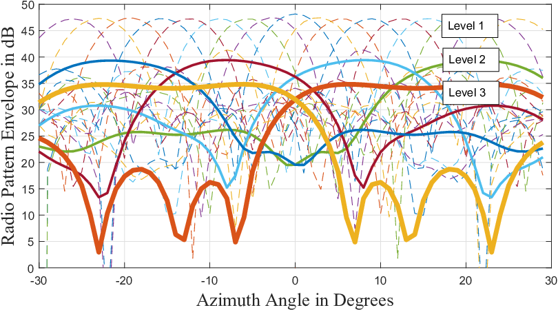
In this paper, we consider a hierarchical beam codebook with $L$ levels of different beam widths for each $i$-th BS AiP and use the notation $\varphi_{k}^{[\ell]}\in[-\pi,\pi]$ with $\ell=1,2,\ldots,L$ and $k=1,2,\ldots,K_{\ell}$ to represent the center angle of the $k$-th beam at the $\ell$-th level. The latter angles at each $\ell$-th level are assumed indexed in increasing values in the angle set $\mathbb{K}_{\ell}$; clearly, ${\rm card}(\mathbb{K}_{\ell})=K_{\ell}$ and $\sum_{\ell=1}^{L}K_{\ell}={\rm card}(\mathbb{F}_{\rm bs})$. We also use hereinafter the notation $\mathbf{u}_{i}(\varphi_{k}^{[\ell]})$ to represent the BF vector realizing the beam in the $\ell$-th level centered at $\varphi_{k}^{[\ell]}$. Without loss of generality, we assume that the first level contains the beams in the hierarchical beam codebook with the narrowest widths (e.g., DFT beams), while the $L$-th level includes the FTBs with the largest widths. Beams resulting from angles of the lower levels are usually included into beams centered at upper levels’ angles. We use notation $\mathbb{M}_{k,i}^{[\ell]}$ to represent the angle set in the $\ell$-th codebook covered by the $k$-th FTB of the $(\ell+1)$-th level codebook at $\varphi_{k}^{[\ell+1]}$. Figure 2 depicts an example hierarchical beam codebook with $L=3$ including two levels of FTBs with different widths and steering angles for a $16\times 16$ URA. As shown in the figure, each beam resulting from angles in $\mathbb{K}_{3}$ shares common coverage with approximately $2$ beams from angles in $\mathbb{K}_{2}$, which in turn have overlapping coverage with $4$ beams from angles in $\mathbb{K}_{1}$. For example, the weights for the second from the left FTB centered at the $\mathbb{K}_{2}$ angle $\varphi_{2}^{[2]}=-8^{\circ}$ were obtained using the following $16\times 16$ weight matrix:

which highlights the link between a radiating element position and its corresponding weight. The analog BF vector for this URA beam can be obtained by simply stacking $\mathbf{W}(\varphi_{2}^{[2]})$’s elements into a column vector with $16^{2}=256$ elements. If this analog beam is deployed in all $M_{\rm bs}$ BS AiPs, then it suffices to set $\mathbf{u}_{i}(\varphi_{2}^{[2]})={\rm vec}(\mathbf{W}(\varphi_{2}^{[2]}))$ in (1) $\forall$$i=1,2,\dots,M_{\rm bs}$.

By considering reciprocal UL and DL communications, we assume that at the first TTI (i.e., upon BM initialization), the beam searching commences in the DL direction using the $K_{1}$ narrow beams of the first level for each BS AiP. Specifically, at the first CTS of this TTI, all $M_{\rm bs}$ AiPs transmit simultaneously orthogonal pilot symbols (i.e., SRSs) to the UE using a narrow beam centered at $\varphi_{1}^{[1]}$; in particular, each $i$-th BS AiP beamforms in the analog domain its pilot symbols with $\mathbf{u}_{i}(\varphi_{1}^{[1]})$. Consequently, the UE measures the SNR at each of its $N_{\rm ue}$ antenna branches for the pilot symbols received by each BS AiP. Then, it computes the summation of the SNR values from all UE antennas referring to each $\mathbf{u}_{i}(\varphi_{1}^{[1]})$ of the $i$-th BS AiP. We term each of the latter summations as $\gamma_{i}(\varphi_{1}^{[1]})$, which actually represents the output SNR with Maximal Ratio Combining (MRC) at the UE. Finally, the quantity $\sum_{i=1}^{M_{\rm bs}}\gamma_{i}(\varphi_{1}^{[1]})$ is compared to the SNR threshold $\gamma_{{\rm th}}$, which refers to the link’s Quality-of-Service (QoS) requirement. In general, $\gamma_{{\rm th}}$ may change with the evolution of TTIs, implying time varying QoS requirements; this can be straightforwardly incorporated to the proposed approach. If $\gamma_{{\rm th}}$ is met with the latter AiPs’ configuration, beam alignment is achieved at this first CTS of the first TTI, and the UE notifies the BS to realize $\mathbf{u}_{i}(\varphi_{1}^{[1]})$ at each $i$-th BS AiP for the upcoming UL data transmission. For this data communication, the UE first estimates the beamformed DL MIMO channel $\mathbf{H}^{\rm H}\mathbf{U}_{\rm RF}\in\mathbb{C}^{N_{\rm ue}\times M_{\rm bs}}$ from pilot symbols and then applies Maximal Ratio Transmission (MRT). However, if $\gamma_{\rm th}$ is not satisfied with $\mathbf{u}_{i}(\varphi_{1}^{[1]})$’s, the remaining $K_{1}-1$ beams of $\mathbb{K}_{1}$ are searched sequentially until an acceptable AiPs’ configuration is identified, or the maximum allowable number of CTSs is reached. During the latter repetitive procedure, the UE is considered capable of storing $\gamma_{i}(\varphi_{j}^{[1]})$ for each $i$-th BS AiP and for each $j$-th realized angle (with $j=1,2,\ldots$) within each TTI. It hence considers, at each $j$-th CTS, the AiPs’ configuration yielding the maximum received SNR up to this slot in the comparison with the SNR threshold $\gamma_{{\rm th}}$.

The previously described BM initialization resulted in the BS AiPs’ configuration $\mathbf{u}_{i}(\varphi_{\nu_{i,1}}^{[1]})$ for each $i$-th BS AiP, where notation $\nu_{i,\ell}$ represents the angle index in the $\ell$-th level angle set $\mathbb{K}_{\ell}$. This analog combining is used till an UL beam misalignment event is identified, which means that the QoS requirement is not met. Suppose that this happens at the $(t+1)$-th TTI triggering the proposed multi-level BM approach summarized in Algorithm 1 for $L=3$, which incorporates an UL phase with narrow beam sweeping followed by a DL phase with $3$-level hierarchical beam searching, if necessary. It is noted that the latter phase can be trivially modified to $L$-level beam searching with $L=2$ or $L>3$. As per the 5G NR limitations [29], UL beam sweeping spans the first $4$ CTSs of each $(t+1)$-th TTI, during which the BS searches over $4$ analog combining vectors in the first level beam codebook for all its AiPs. The sequence of the $4$ angles to be swept for the latter vectors is designed using Algorithm 2, which targets analog combining searching over adjacent angles to those decided for the previous $t$-th TTI. In particular, for each $i$-th AiP, this algorithm computes the angle sweeping sequence vector $\mathbf{m}_{i}^{[\ell]}$ having ${\rm card}\left(\mathbb{K}_{\ell}\right)-1$ elements referring to the angles’ indices; the angle index used in the previous $t$-th TTI is excluded.

In Step $4$ of Algorithm 1, the instantaneous received SNR at the end of each $j$-th CTS at each $i$-th BS AiP that realizes the analog BF vector $\mathbf{u}_{i}(\varphi_{[\mathbf{m}_{i}]_{j}}^{[1]})$ is calculated as

Next, at the end of each $4$-th CTS of each $(t+1)$-th TTI, the maximum received SNR for each $i$-th BS AiP is obtained as

and the quantity $\sum_{i=1}^{M_{\rm bs}}\gamma_{i}$ is calculated and finally compared to the SNR threshold value $\gamma_{\rm th}$. If this performance threshold is met, beam alignment is achieved with the BS AiPs’ configuration yielding $\gamma_{i}$’s; we denote the first level beam angle yielding $\gamma_{i}$ for the $i$-th BS AiP by $\varphi_{[\mathbf{m}_{i}]_{\rm max}}^{[1]}$. Otherwise, the DL BM phase of Algorithm 1 is followed, which includes our novel $3$-level hierarchical beam searching.

References

- [1] T. S. Rappaport, S. Sun, R. Mayzus, H. Zhao, Y. Azar, K. Wang, G. Wong, J. K. Schulz, M. Samim, and F. Gutierrez, “Millimeter wave mobile communications for 5G cellular: It will work!” IEEE Access, vol. 1, pp. 335–349, May 2013.
- [2] I. F. Akyildiz, C. Han, and S. Nie, “Combating the distance problem in the millimeter wave and terahertz frequency bands,” IEEE Commun. Mag., vol. 55, no. 6, pp. 102–108, Jun. 2018.
- [3] “IEEE wireless LAN MAC and PHY specifications– Amendment 3: Enhancements for very high throughput in the 60 GHz band,” IEEE Std. 802.11ad, 2012.
- [4] 3GPP, “Study on New Radio (NR) Access Technology- Physical Layer Aspects- Release 14,” TR 38.802, 2017.
- [5] V. Venkateswaran and A.-J. van der Veen, “Analog beamforming in MIMO communications with phase shift networks and online channel estimation,” IEEE Trans. Signal Process., vol. 58, no. 8, pp. 4131–4143, Aug. 2010.
- [6] C. H. Doan, S. Emami, D. A. Sobel, A. M. Niknejad, and R. W. Brodersen, “Design considerations for 60 GHz CMOS radios,” IEEE Commun. Mag., vol. 42, no. 12, pp. 132–140, Dec. 2004.
- [7] X. Zhang, A. F. Molisch, and S.-Y. Kung, “Variable-phase-shift-based RF-baseband codesign for MIMO antenna selection,” IEEE Trans. Signal Process., vol. 53, no. 11, pp. 4091–4103, Nov. 2005.
- [8] A. F. Molisch, V. V. Ratnam, S. Han, Z. Li, S. L. H. Nguyen, L. Li, and K. Haneda, “Hybrid beamforming for massive MIMO: A survey,” IEEE Commun. Mag., vol. 55, no. 9, pp. 134–141, Sep. 2017.
- [9] A. Alkhateeb, O. E. Ayach, G. Leus, and R. W. Heath, Jr., “Channel estimation and hybrid precoding for millimeter wave cellular systems,” IEEE J. Sel. Topics Signal Process., vol. 8, no. 5, pp. 831–846, Oct. 2014.
- [10] Z. Marzi, D. Ramasamy, and U. Madhow, “Compressive channel estimation and tracking for large arrays in mm-wave picocells,” IEEE Trans. Signal Process., vol. 11, no. 3, pp. 514–527, Apr. 2016.
- [11] A. Bazzi, D. T. M. Slock, L. Meilhac, and S. Panneerselvan, “A comparative study of sparse recovery and compressed sensing algorithms with application to AoA estimation,” in Proc. IEEE SPAWC, Edinburgh, UK, 3-6 Jul. 2016, pp. 1–5.
- [12] G. C. Alexandropoulos and S. Chouvardas, “Low complexity channel estimation for millimeter wave systems with hybrid A/D antenna processing,” in Proc. IEEE GLOBECOM, Washington D.C., USA, 4-8 Dec. 2016, pp. 1–6.
- [13] E. Vlachos, G. C. Alexandropoulos, and J. Thompson, “Massive MIMO channel estimation for millimeter wave systems via matrix completion,” IEEE Signal Process. Lett., vol. 25, no. 11, pp. 1675–1679, Nov. 2018.
- [14] ——, “Wideband MIMO channel estimation for hybrid beamforming millimeter wave systems via random spatial sampling,” IEEE J. Sel. Topics Signal Process., vol. 13, no. 5, pp. 1136–1150, Sep. 2019.
- [15] H. Zhang, S. Venkateswaran, and U. Madhow, “Channel modeling and MIMO capacity for outdoor millimeter wave links,” in Proc. IEEE WCNC, Sydney, Australia, 18-21 Apr. 2010, pp. 1–6.
- [16] S. Hur, T. Kim, D. J. Love, J. V. Krogmeier, T. A. Thomas, and A. Ghosh, “Millimeter wave beamforming for wireless backhaul and access in small cell networks,” IEEE Trans. Commun., vol. 61, no. 10, pp. 4391–4403, Oct. 2013.
- [17] K. Hosoya, N. Prasad, K. Ramachandran, N. Orihashi, S. Kishimoto, S. Rangarajan, and K. Maruhashi, “Multiple sector ID capture (MIDC): A novel beamforming technique for 60 GHz band multi-Gbps WLAN/PAN systems,” IEEE Trans. Antennas Propag., vol. 63, no. 1, pp. 81–96, Jan. 2015.
- [18] J. Wang, Z. Lan, C.-W. Pyo, T. Baykas, C.-S. Sum, M. A. Rahman, J. Gao, R. Funada, F. Kojima, H. Harada, and S. Kato, “Beam codebook based beamforming protocol for multi-Gbps millimeter-wave WPAN systems,” IEEE J. Sel. Areas Commun., vol. 27, no. 8, pp. 1390–1399, Oct. 2009.
- [19] C. Jeong, J. Park, and H. Yu, “Random access in millimeter-wave beamforming cellular networks: Issues and approaches,” IEEE Commun. Mag., vol. 53, no. 1, pp. 180–185, Jan. 2015.
- [20] C. Barati, S. A. Hosseini, S. Rangan, P. Liu, T. Korakis, S. S. Panwar, and T. S. Rappaport, “Directional cell discovery in millimeter wave cellular networks,” IEEE Trans. Wireless Commun., vol. 14, no. 12, pp. 6664–6678, Dec. 2015.
- [21] V. Raghavan, J. Cezanne, S. Subramanian, A. Sampath, and O. Koymen, “Beamforming tradeoffs for initial UE discovery in millimeter-wave MIMO systems,” IEEE J. Sel. Topics Signal Process., vol. 10, no. 3, pp. 543–559, Apr. 2016.
- [22] G. C. Alexandropoulos, “Position aided beam alignment for millimeter wave backhaul systems with large phased arrays,” in Proc. IEEE CAMSAP, Curaçao, Dutch Antilles, 10-13 Dec. 2017, pp. 1–5.
- [23] I. Aykin and M. Krunz, “Efficient beam sweeping algorithms and initial access protocols for millimeter-wave networks,” IEEE Trans. Wireless Commun., vol. 19, no. 4, pp. 2504–2514, Apr. 2020.
- [24] J. Song, J. Choi, and D. J. Love, “Common codebook millimeter wave beam design: Designing beams for both sounding and communication with uniform planar arrays,” IEEE Trans. Wireless Commun., vol. 65, no. 4, pp. 1859–1872, Apr. 2017.
- [25] M. Akdeniz, Y. Liu, M. Samimi, S. Sun, S. Rangan, T. Rappaport, and E. Erkip, “Millimeter wave channel modeling and cellular capacity evaluation,” IEEE J. Sel. Areas Commun, vol. 32, no. 6, pp. 1164–1179, June 2014.
- [26] Y. P. Zhang and D. Liu, “Antenna-on-chip and antenna-in-package solutions to highly integrated millimeter-wave devices for wireless communications,” IEEE Trans. Antennas Propag., vol. 57, no. 10, pp. 2830–2841, Oct. 2009.
- [27] P. Kyosti et al., “WINNER II channel model,” Technical Report IST-WINNER D1.1.2 ver 1.1, Sept. 2007.
- [28] R. J. Mailloux, Phased Array Antenna Handbook, New York, 2004.
- [29] M. Giordani, M. Polese, A. Roy, D. Castor, and M. Zorzi, “A tutorial on beam management for 3GPP NR at mmWave frequencies,” IEEE Commun. Surveys Tuts, vol. 21, no. 1, pp. 173–196, 2019.
- [30] M. Rebato, L. Rose, and M. Zorzi, “Performance assessment of MIMO precoding on realistic mmWave channels,” in Proc. IEEE ICC, Shanghai, China, 20-24 May 2019, pp. 1–6.
- [31] C. Huang, A. Zappone, G. C. Alexandropoulos, M. Debbah, and C. Yuen, “Reconfigurable intelligent surfaces for energy efficiency in wireless communication,” IEEE Trans. Wireless Commun., vol. 18, no. 8, pp. 4157–4170, Aug. 2019.
- [32] N. Shlezinger, G. C. Alexandropoulos, M. F. Imani, Y. C. Eldar, and D. R. Smith, “Dynamic metasurface antennas for 6G extreme massive MIMO communications,” to appear, 2021, [online] https://arxiv.org/abs/2006.07838.