Graph complements of circular graphs
Abstract.
In this report, we study graph complements of cyclic graphs or graph complements of path graphs. are circulant, vertex-transitive, claw-free, strongly regular, Hamiltonian graphs with a symmetry and Shannon capacity . Also the Wiener and Harary index are known. The explicitly known adjacency matrix spectrum leads to explicit spectral zeta function and tree or forest quantities. The forest-tree ratio of converge to in the limit when goes to infinity. The graphs are all Cayley graphs and so Platonic in the sense that they all have isomorphic unit spheres . The graphs are homotop to wedge sums of two -spheres and are homotop to -spheres, are contractible, are homotop to -spheres. Since disjoint unions are dual to Zykov joins, graph complements of all -dimensional discrete manifolds are homotop to either a point, a sphere or a wedge sums of spheres. If the length of every connected component of a 1-manifold is not divisible by , the graph complement of must be a sphere. In general, the graph complement of a forest is either contractible or a sphere. It also follows that all induced strict subgraphs of are either contractible or homotop to spheres. The f-vectors or satisfy a hyper Pascal triangle relation, the total number of simplices are hyper Fibonacci numbers. The simplex generating functions are Jacobsthal polynomials, generating functions of -king configurations on a circular chess board. While the Euler curvature of circle complements is constant by symmetry, the discrete Gauss-Bonnet curvature of path complements can be expressed explicitly from the generating functions. There is now a non-trivial -periodic Gauss-Bonnet curvature universality in the complement of Barycentric limits. The Brouwer-Lefschetz fixed point theorem produces a -periodicity of the Lefschetz numbers of all graph automorphisms of . There is also a -periodicity of Wu characteristic. This corresponds to -periodicity in dimension as is homotop to a suspension. These are all manifestations of stable homotopy features, but purely combinatorial.
Key words and phrases:
Complements of Cyclic graphs, Graph Homotopy1991 Mathematics Subject Classification
57M15, 68R10,05C501. Introduction


1.1.
Graph complements of circular graphs are Cayley graphs of the circular group that exhibit surprisingly rich combinatorial, geometric, topological and spectral features. They allow to illustrate results which in the continuum are more technical, like Lefschetz or Gauss-Bonnet theory. Spectral theoretical questions relate to zeta functions and harmonic analysis and eigenvalue problems for various circular matrices associated to the geometry. Fourier theory makes there everything explicit, allowing also to understand graph limits. Combinatorial problems come in when counting subgraphs, like the number of simplices the number of trees or forests or finding numerical quantities like the chromatic number or independence number or when establishing capacity quantities which are pivotal in information theory. The graph complements of cyclic graphs share the symmetry and regularity of the circle graphs but also always have the homotopy types of large dimensional spheres or a wedge sum of two large dimensional spheres. Unit spheres in these graphs are complements of path graphs and are always contractible or spheres. This is exactly what happens in realistic implementations of manifolds like in a computer using floating point arithmetic: if a small accuracy threshold is given, then the spheres of this radius are either homotopy spheres or then contractible. At rational or typical algebraic numbers in an interval for example, the spheres of accuracy are 0-spheres, while for most other numbers the spheres are contractible the simple reason being that a computer can only have represent a finite amount of numbers.
1.2.
Circle graph complements behave in many respects like manifolds or manifolds with boundary; but they are also models in which we allow for homotopy deviations. It is more subtle than homotopy alone as we look also at the homotopy of unit spheres. We deal then with a class of metric spaces which share with Euclidean round spheres or round balls the property that arbitrary intersections of geodesic spheres are either spheres or points. More generally, the union of path graphs or circle graphs each of length not divisible by three all have as graph complement a single high dimensional sphere, always homotopically speaking of course. A consequence is that graph complements of forests are always contractible or spheres. These spaces topologically behave like manifolds or manifolds with boundary. An example is the Moebius strip which is the graph complement of the heptagon which however is homotopically a circle as removing a contractible part renders it contractible. Most amazingly, the Gauss-Bonnet curvature distribution of the graph complement of a large linear graphs show a non-trivial periodic universality. This is a stable homotopy property in that this curvature attractor is invariant under the suspension operation. It is completely unexpected to see an attracting period-6 cycle which consists of non-trivial smooth functions. It leads a period-2 attractor under the Barycentric refinement renormalization map. In general, the curvature on a graph complement of a path graph has three different regions on each of which the curvature converges to a smooth limiting function in the limit. We have not yet analyzed the limiting functions carefully yet but they are given explicitly as hyperelliptic functions for each .
1.3.
Our results are all located entirely within combinatorics. Geometric realizations of the objects could produce classical topological spaces and would allow to see the results into the hart of stable homotopy questions in topology. We would like to stress however that we never really need the continuum. Also the integrals which appear are integrals of polynomials and so could be done without invoking the real line. The linear algebra part entering when looking at cohomology groups or Lefschetz numbers could be done over discrete fields like rational numbers, the eigenfunctions are in finite field extensions of the rationals. Many questions are open. We do not understand yet for example for which trees the graph complement is contractible or what happens for general with graph complements of triangle-free graphs. We know that for forests, the graph complement is either contractible or a sphere. The cyclic graphs are an example and one can look at more general Cayley graphs. If the cyclic graphs which are Cayley graphs of the cyclic group is replaced by graphs which are Cayley graphs of dihedral groups, and which we only looked at briefly yet, we observe a similar story: we get again spheres and wedge sums of spheres. The combinatorial data are still given by more complicated recursions and there is a curvature renormalization limit. The dihedral groups are already non-Abelian. In general, one can look at the graph complements of any finite simple Cayley graph (in a frame work where generators always come also with their inverse so that we have undirected graphs). A natural case not yet studied are the Cayley graphs of product groups equipped with their natural generators producing a grid graph. We then look at the graph complement of such grid graphs. The case is the tesseract. Its graph dual is a wedge sum of six -spheres as the Betti vector of is . But in general, it can be more complex: for already, the graph complement is no more a sphere, nor a bouquet of spheres, as it has Betti vector .
1.4.
This work started with the observation that graph complements of circle graphs are either wedge sums of spheres or spheres. We saw that by computing the cohomology groups for the first few dozen cases. These data can be obtained as null spaces of the Hodge Laplacian for the graph, which is already a square of the Dirac operator [31, 36, 52]. The Hodge method is swiftly done: order the maximal simplices in the Whitney complex of the graph arbitrarily, write down the incidence matrices then build the matrix and look at the kernels of each block. The block corresponding to -functions is the Kirchhoff matrix , where is the diagonal vertex degree matrix and is the adjacency matrix of the graph. Discrete versions of calculus have been reinvented and refined many times, especially in the computer science literature. The basic idea however is already in the original approach of pioneers like Betti or Poincaré, using incidence matrices. Hodge theory brings it down to linear algebra. There is no need for Clifford matrices in the discrete because the Dirac operator is the square root of the Laplacian. The functor giving from an algebra its Clifford algebra is in the discrete implemented by Barycentric refinement, a process which transforms simplices into points on a new level giving rise then to new simplices. In the discrete the exterior algebra is already given in terms of functions on complete subgraphs. The situation is trickier in the continuum, because lower-dimensional parts of a space like a manifold or variety have to be accessed sheaf theoretically.
1.5.
Given an automorphism of the graph , one can look at the action which induces on the kernels on -forms. The later are anti-symmetric functions on -simplices. We can then compute the trace of each block and super sum it up. This gives the Lefschetz number of the graph. By applying the heat operators on the Koopman operator defined by the map, one can immediately see that is the sum of the indices of the simplices (which we think of as points) fixed by . The reason is that by McKean-Singer symmetry, [76, 4, 28], the super trace of for so that is constant in . We have and by Hodge and the fact that the eigenspaces of corresponding to non-zero eigenvalues are washed away, which is a result of having the non-zero eigenvalues being positive. This works without any assumptions whatsoever on the graph and is the reason why the Lefschetz fixed point theory is so simple here. In [29] we gave a different proof closer to Hopf.
1.6.
To digress a bit more, the story looked at first suitable for studying homotopy groups of spheres numerically: when adding two homotopies on a sphere, we realize the two on the two sides of the wedge sum, then lift it to the sphere which can be seen as a ramified cover of the wedge sum along the equator. A naive idea is to place sphere structures onto groups and have so spheres act more conveniently on spheres. We indeed see here sphere structures on Cayley graphs of cyclic groups and since can act on , we can have spheres acting on spheres. It seems not yet to help to compute the homotopy groups of spheres but this is also not to be expected as homotopy groups of spheres are a difficult problem. However, the story is of independent interest in graph theory. We also want to use it to illustrate the use of graphs to study topology. The already mentioned Lefschetz story. It implies for example that if is a contractible graph, then any automorphism must have a fixed simplex. This is a discrete Brouwer fixed point theorem. Verifying Brouwer using discrete models has tradition [12].
1.7.
The study of the topology of graph complements in general appears to be a vastly unexplored area. That graph complements of cyclic graphs are already rich can surprise. In the future, we would like to know what happens in general with graph complements of times Barycentric refined graphs . In one dimension, there is a limited class of topological spaces which appear: we get spheres and points (meaning contractible spaces). The topology is much richer in higher dimensions and still deserves to be explored further. The Betti vectors of for example is , for already and for the Betti vector is and the Euler characteristic is . Also for general circulant graphs like the self-complementary Paley graphs (quadratic reciprocity), rich topologies can appear. The Paley graph to the prime p=13 is a flat discrete torus is a manifold with zero curvature and so a discrete Clifford torus. We have not found larger Paley graphs yet that produce discrete manifolds. Which graph complements of forests are points, which are spheres? Observed and not proven is also that the normalized spectrum of the Hodge operator of converges. It does so for the [43]. Also the structure of spectral zeta functions deserves more attention. There are inverse problem of relating the spectrum to the graph. An example of a result is that is the ratio of rooted forests over rooted trees, a direct consequence of the matrix tree and matrix forests theorems. We plan to write about this more in the future but will mention the tree-forest ratio already here as it diverges for in the limit but converges to in the case of its complement for .
1.8.
In order to illustrate the upcoming story, let us in this introduction take a concrete example and look at the graph complement of . This graph is obtained by drawing all the diagonals in a -gon. The graph is a pretty inauspicious geometric object, consisting of vertices and edges. It can be seen as the Cayley graph of , where we take as generators the complement of the usual generators . There is more structure beyond this one-dimensional simplicial complex skeleton of . There are triangles, tetrahedra (complete subgraphs with 4 vertices) and 11 hyper tetrahedra (complete subgraphs of 5 vertices). As we will see below, the f-vector is a row in a hyper Pascal triangle and the sum , counting all the simplices in the graph is a hyper Fibonacci number satisfying the recursion with initial condition . The Euler characteristic of is . In general, we will see . Gauss-Bonnet tells that this is the sum of curvatures but because of the transitive automorphism group the curvature at every vertex of is constant . By the general Gauss-Bonnet result, the curvature is an anti-derivative of the simplex generating function of the unit sphere . In our case, the unit spheres are all complements of graph paths .
1.9.
Let us dwell on this a bit more as it also brings us to the hart of the matter. First of all, the curvature of itself is not that interesting because it is constant: we have a transitive symmetry group on and so a constant Gauss-Bonnet curvature , because is the number of vertices. In some sense, behaves like a round sphere in the continuum, where in the even-dimensional case, we can write down immediately the Gauss-Bonnet-Chern integrand without computing the Riemann curvature tensor simply because by symmetry, the curvature is constant. For odd-dimensional manifolds, the Gauss-Bonnet-Chern curvature is not even defined and usually assumed to be zero, as the Euler characteristic is zero for manifolds for which Poincaré-Duality holds. We were 10 years ago first puzzled to see the discrete curvature always to be constant zero for odd-dimensional discrete manifolds [23].We proved it soon after with integral geometric methods seeing curvature as an expectation of Poincaré-Hopf indices and quite recently also saw it as a simple manifestation of Dehn-Sommerville [59]. In our case, we have unit spheres in which are graph complements of path graphs which even in the odd-dimensional case have a non-trivial curvature (which actually is universal in the limit ). This is not a contradiction, because we deal in the case of or with “fuzzy spheres” which mathematically means that we have spheres modulo homotopy. But not only that also the unit spheres of these spaces are either spheres or contractible.
1.10.
From a differential geometric point of view, the graphs are more interesting: the curvature is not constant. We therefore started also to investigate more the curvature of the path graph complements . Curvature is most elegantly described using the simplex generating functions. In full generality, the simplex generating function of a graph is the sum of the anti-derivatives of the simplex generating functions of the unit spheres. The later are the curvature functions which when evaluated at the parameter produce Euler characteristic and so the Gauss-Bonnet theorem. One might now have the impression that this curvature is a discrete combinatorial oddity. But it actually is the real thing. Integral geometric considerations show that this curvature is the analogue of Gauss-Bonnet-Chern in the case when the graphs are triangulations of an even-dimensional compact Riemannian manifold. If we make a finer Regge triangulation of a compact Riemannian manifold and realize both the graph as well as the manifold in a larger dimensional Euclidean space which is possible by Nash’s embedding theorem, then we can look at the curvature obtained by the index expectation of Morse functions given by linear functions in . There is a natural Haar measure making this a nice rotationally symmetric probability measure of functions. The induced curvature on is Gauss-Bonnet-Chern. The induced curvature on is an index expectation curvature on the graph. High dimensional embedding considerations lead to the Levitt curvature we consider.
1.11.
In our case, for the graphs or , the simplex generating functions satisfy a recursion relation and will be identified as Jacobsthal polynomials. The recursion for is with [17, 82] For , we have the same recursion with . We also know in the same way the simplex generating functions of the unit spheres of . As the graphs have constant curvature and the Euler characteristic is known, it follows from Gauss-Bonnet that . For example, (there are three vertices and one edge) integrates to on . But is the unit sphere of , a graph that is homotopic to the figure 8 and so has Euler characteristic with curvatures . It is curious that Gauss-Bonnet produces a relation for a sequence of recursively defined polynomials.


1.12.
We have already mentioned that the unit spheres in are all graph complements of linear graphs with vertices. While are wedge sums of two -spheres and are -spheres, the unit spheres of are -spheres and are contractible. All unit sphere of for example are homotopic to -spheres. Any intersection of two or more disjoint unit spheres in is always a -sphere or contractible. If we look at unit spheres of unit spheres in , then these are graph complements of disjoint unions of linear graphs and therefore joins of spheres or contractible graphs and so spheres or contractible graphs. In other words, intersections of an arbitrary collection of unit spheres in always are either spheres or points. One can rephrase this and say that these are spaces of Lusternik-Schnirelmann category 1 or 2 [18]. Since we also know that the graph complements of star graphs are -spheres, we can glue star graphs linear graphs and circular graphs together and get the topology of the total. For trees of forests, the graph complements always are either contractible or spheres, graphs of category 1 or 2. We deal with a class of graphs for which the unit spheres are in the same class.
1.13.
Let us add a bit more on the use of graph theory in topology. Maybe because the origins of graph theory were “humble, even frivolous” to quote [78], it is tempting to dismiss higher dimensional topological features in graphs at first. Already Euler, who first considered graphs as a tool to study topological features of a two-dimensional map of St Petersburg and so looked beyond one dimension and seen graph theory as part of topology. Also early topologists like Hassler Whitney who worked both in graph theory as well as the foundations for modern differential topology would not look at a graph as just one-dimensional simplicial complex but think about the clique complex it defines. Indeed, the simplicial clique complex consisting of all subsets of the vertex set of a graph is today also called the Whitney complex of the graph. For , it produces a -dimensional topological space if realized in Euclidean space. From the homotopy point of view, it is a three dimensional sphere.
1.14.
The hyper hyper-tetrahedra in do not generate the topological realization yet. The space is not “manifold-like”. But if we include the tetrahedra which are not contained in maximal hyper-tetrahedra, then this generates the full simplicial complex , the geometric realization of the Whitney complex of . 11 1 We usually do not bother with geometric realizations but stay within finite combinatorics. The smallest example of a graph with an impure simplicial complex is the graph , It features vertices, edges and triangles. The two triangles as well as the 3 edges connecting them generate the complex. They form a prism. Traditionally, one would look at this as a model for a -sphere but this is not what it is when looking at the Whitney complex. The three squares are not present in the geometric realization of the Whitney complex. Including such faces comes natural in the context of topological graph theory [13] but especially in higher dimensions has led to much confusion. We have which reflects the fact that we have a 2-sphere in which 3 holes are present. The book [73] is dedicated to the confusion and [80, 15] explains this further. Things are crystal clear if one insists on looking at simplices (complete subgraphs) as the faces of a polyhedron and refer to discrete CW complex structures when building up polyhedra more effectively with as few cells as possible (i.e. appearing in [66].


1.15.
If we shrink the triangles in to a point, we get a graph with two squares glued together. The shrinking process is what one calls a homotopy. Unlike homeomorphisms, homotopies can transcend dimension. The maximal dimension of is but it is homotopic to a curve of maximal dimension . You might have noticed that the topological space is homotopic to a figure complex which is a lemniscate. It is a curve which is a variety and not a manifold. Its Euler characteristic is as should be for a curve of genus as there are two holes. One calls the figure graph also the wedge sum of two circles or a “bouquet of circles”. The wedge sum of spheres is important as it is the crux to define the addition in the homotopy groups of spheres. If are continuous maps from a pointed topological space to the pointed topological space , then one has a natural map . As is a branched cover of where the ramification happens on the equator, one can lift to getting again a continuous map from . This addition is the operation in the homotopy groups . The structure of these groups is still not fully understood. Having small models for spheres and wedge sums of spheres can be a major motivation for what we do here.
1.16.
All the cohomology groups of can be computed quickly finite linear algebra. The ’th cohomology group is the kernel of the Hodge Laplacian matrix , where is the Dirac operator which is in the case a matrix. The matrix is the exterior derivative. It maps functions on -simplices to functions on -simplices. We have to chose an order on each simplex to define the map, but changing such an order on a simplex is just a change of the coordinates and so a base change which does not affect the kernel and so the cohomology. The Hodge approach to cohomology is rewarding because we get more than just an abstract answer but concrete harmonic forms, solutions to the Laplace equation . In the case , there is a harmonic form on -forms, the constant function. All connected graphs just have one such harmonic form. But then there is the harmonic -form. Because is an integer matrix, it can be represented by an integer vector. In this case it takes values in .
1.17.
The exterior derivatives were called incidence matrices by Poincaré and have all the same properties than the exterior derivatives in the continuum. For a scalar function of the graph , it produces the gradient For a function , the exterior derivative is the curl , where is the set of triangles. The matrix is block diagonal, where each block operators on -forms. The operator is the Kirchhoff Laplacian, the analogue of the scalar in calculus. We have studied graph complements of cyclic graphs first in order to compute cohomology groups and spectra of . We notice for example that the Hodge spectrum converges to a limit for but we have not yet proven such a sphere central limit theorem.
1.18.
Triangulations of -spheres can be realized as finite abstract simplicial complexes which are Whitney complexes of graphs defined by points. The -sphere for example is realized by the octahedron graph, the -sphere, also known as the -cell is realized on a set with points. These small simplicial complexes are the smallest triangulations of these manifolds and so most economical. (-simplices are not spheres in this frame work because simplices are contractible and so points. Only the -skeleton complex of the Whitney complex of a simplex is a sphere.) The cross polytopes just mentioned are models of spheres that have high symmetry. They are Platonic solids in arbitrary dimension and constant curvature , where and is the set of dimensional simplices in a graph and is the unit sphere of . In the case of a -sphere realized by the graph we have on each vertex. The graphs share with cross polytopes the property that they are very small and also have a lot of symmetry. The cross polytopes are circulant graphs obtained by taking the complete graph and deleting the large diagonals. Cross polytopes are graphs complements of -dimensional graphs. They are the complement graphs of disjoint graphs. But we have more with the graphs as we also have small implementations of wedge sums.
1.19.
As in classical topology, the wedge sum of two spheres is no more a manifold. in classical frame works it can be realized as a variety with one singular point, the point where the spheres touch. For , we get the lemniscate. When discretizing this, we can glue two cross polytopes together at a point and so get a simplicial complex complex with points. If we look at homotopic equivalents only, one can even do with points. For the circle for example one can glue together two circular graphs along an edge and get the digital figure-8 curve. But this implementation does not have constant curvature. It is on the two middle points and else, adding up to the Euler characteristic . This persists in higher dimensions. Note that Gauss-Bonnet works for arbitrary graphs and that just in the case of even dimensional discrete manifolds, it goes in a limit to the Gauss-Bonnet-Chern theorem known in differential geometry.
1.20.
It might surprise a bit that we realize a homotopy -sphere or a wedge sum in such a way that the curvature is constant and even keep the Platonic property of having isomorphic unit spheres everywhere with a transitive symmetry group. The graphs are constant curvature graphs and the ability to look at homotopic graphs allowed to get more symmetry. For every notion of sectional curvature which only depends on unit spheres we have the same curvature spectrum at every vertex. The graph for example which is homotopic to a wedge sum , has constant Euler curvature because the wedge sum of two spheres has Euler characteristic and the curvatures must be constant on each of the 12 vertices. There is therefore a differential geometric angle to the story. We will also see a differential topological aspect when building up the graphs or the dual graphs of linear graphs. Indeed, curvature can be seen as the expectation of Poincaré-Hopf indices and the later can be seen as Euler characteristic changes when adding cells during a build-up. In our case, we can see the sequence as a Morse build-up as the change of Euler characteristic is or there.
1.21.
Euclid’s geometry of the Euclidean space is primarily a story of circles and lines. If graph theory is used as a tool to study geometry in arbitrary dimensions, there is no natural notion of “lines” or linear spaces or tangent spaces. Even geodesics are in general not unique already for points of distance two apart. There is however a theory of spheres. Given a graph, there is a notion of unit spheres which are the subgraphs generated by the vertices adjacent to a vertex . As a consequence of the fact that the graphs and have diameter for the intersection of two unit spheres is always non-empty and of the form which are homotopic to balls of spheres. The graphs share an important property which holds in Euclidean spaces or round spheres: the intersection of an arbitrary number of geodesic unit spheres is either a point or a sphere. In the discrete, this is a property we know from discrete manifolds. If we define a -manifold as a graph which has the property that every unit sphere is a -sphere and a -sphere is a -manifold which becomes contractible when removing a vertex, then by induction, the intersection of an arbitrary number of unit spheres is either a point or a sphere.
2. Combinatorics
2.1.
The graph complements of cyclic graphs are circulant graphs of diameter . It is usually denoted as but we write . We can see every circulant graph as the undirected Cayley graph of a presentation of in which a set of generators together with its inverses are given. Then is with generators while is with generators . Whenever we look at the topology and homotopy of the finite simple graph , we refer to the topology of the Whitney complex of this graph. This is the finite abstract simplicial complex formed by the complete subgraphs of . The maximal dimension of is then the dimension of the largest simplex in . It is . For for example, where the maximal dimension is while for the maximal dimension is already because two triangles appear. A topological question for is equivalent to asking the same question for a geometric realization of in Euclidean space. Then is a circle and consists of two triangles with corresponding vertices connected. Examples of quantitative numbers are the Betti numbers, the dimensions of the cohomology groups, the homotopy groups. For for example which is homotopic to a figure 8 and so a wedge sum of two circles, the Betti vector is and the fundamental group is the free group with two generators.
2.2.
Let us first look at the combinatorial question to determine the number of -dimensional faces (simplices, cliques) in . We can build up the simplices inductively. If we know the -simplices in , they produce also -simplices in . Additionally, any -simplex in can be joined with a new vertex to get a simplex in . This immediately leads to the recursion
They are known as hyper Pascal triangle relations. It is a direct consequence from the set-up. We can build the Whitney complex recursively by joining the Whitney complex of and adding an augmented version of the complex of because there is then space for a new vertex. The number facets=maximal simplices=maximal cliques is either or , depending on whether is even or odd. The numbers giving the number of complete subgraphs of forms a sequence called the hyper Fibonacci numbers. They satisfy the recursion
In our case, the initial condition are which gives etc. Unlike the Euler characteristic formula which is periodic for only, the numbers make sense as the total clique number for all with . For we have with and for , we have the empty graph with . For as is the 2 point graph which is the -sphere and on as is the 3-point graph without edges which is .
| 0 | 1 | 0 | |||||
| 1 | 1 | 0 | 1 | ||||
| 2 | 2 | 2 | 2 | ||||
| 3 | 3 | 3 | 3 | ||||
| 4 | 4 | 2 | 6 | 2 | |||
| 5 | 5 | 5 | 10 | 0 | |||
| 6 | 6 | 9 | 2 | 17 | -1 | ||
| 7 | 7 | 14 | 7 | 28 | 0 | ||
| 8 | 8 | 20 | 16 | 2 | 46 | 2 | |
| 9 | 9 | 27 | 30 | 9 | 75 | 3 | |
| 10 | 10 | 35 | 50 | 25 | 2 | 122 | 2 |
| 11 | 11 | 44 | 77 | 55 | 11 | 198 | 0 |
2.3.
In the above table, is the only non-sphere or non-wedge sum of spheres. The formula only starts to apply for and only really makes sense geometrically for as for we have the complement of which is the graph with 3 vertices and no edges. Let us summarize this
Theorem 1 (Hyper Pascal).
The components of the vector of satisfy the hyper Pascal relation. The total number of simplices in is the ’th hyper Fibonacci number.
Proof.
Use induction with respect to . When going from to , we pick a polar pair , add the edge , add a new vertex and connect it to all points except . All the old -simplices from remain. Additionally there is a -simplex for any -simplex in . ∎
2.4.
A consequence is that we know the Euler characteristic
explicitly for :
Corollary 1 (6-periodicity of Euler characteristic).
The Euler characteristic of is for .
The Euler characteristic of is for .
Proof.
Also this can be obtained by induction using the explicit recursion.
The formula only makes geometric sense for . For , we think of
as the 0-sphere, a 2-vertex graph without edges.
An other proof can be done by using the explicit formula for the
Jacobsthal polynomial to which we come next.
The 6-periodicity comes from the fact that is
homotopic to a suspension and that the Euler characteristic of spheres is
2-periodic switching between and . The least common denominator of
and is then .
∎
2.5.
For a general graph , the simplex generating function
has the property that it multiplies , if is the join of the graphs and . The join in graph theory is often denoted as the Zykov join because it was first introduced by Zykov into graph theory [85] but it does exactly have the same properties as in topology. The join with the zero sphere, a 2-point graph without vertices, is then a suspension.
2.6.
The simplex generating function of and the simplex generating function of are given by Jacobsthal polynomials:
Lemma 1 (Jacobsthal).
The simplex generating functions of and of satisfy the recursion
They are solved by the explicit formulas
Proof.
This follows from the Hyper-Pascal relations. While the values for and do not have a direct interpretation, they can back traced from the relation. The explicit formulas are obtained using linear algebra similarly as the explicit Binet formula for Fibonacci numbers are obtained: with an Ansatz one gets a basis solution or . One can then fix the constants to match the initial condition. ∎
3. Homotopy spheres and wedge sums
3.1.
A topological question is to determine the homotopy type of the topological space obtained from when we realize it as a Whitney complex. For more on discrete graph homotopy see [64]. The graphs are a test case to see how far we can go with computing all the cohomology groups using Hodge theory. That is how we got to these graphs. When we looked at small cases and computed the cohomology up to , we noticed that in all cases we have homology spheres or homology wedge sums of two spheres. We proved then the following theorem:
Theorem 2 (Sphere bouquet theorem).
is homotopic to a wedge sum of two -spheres while and are both homotopic to -spheres.
Proof.
Since in the dual picture is an edge refinement and the suspension is (adding two disjoint points), we see that the two operations commute. Indeed, modulo homotopies the operation is a cube root of the suspension as the suspension of the wedge sum of two spheres is a wedge sum of two higher dimensional spheres. To prove this, look at the transitions for to . Now pick a and look at its equator obtained by removing the vertices , then this is by induction either a lower dimensional sphere or lower dimensional wedge sum of two spheres. If we make the extension the by induction transforms to a higher dimensional space of the same type. Since is a suspension of and is a suspension of we by induction know that also on level , the correct extension is done also on the next level.
In order to see what happens we split up the transition and verify that it is a composition of suspension and homotopies. Since the transition happens for by taking a disjoint union of with the path graph (which has a dual which is homotopic to a 0-sphere so that we have in the dual a suspension), then snapping one of the edges in and connecting , then (which are all homotopies when seen on the side), we see that is a suspension modulo homotopies. ∎

3.2.
Observe that if we take any unit sphere in and remove the edge , if was the sphere of radius in we end up with a graph which is isomorphic to . It so happens that and are homotopic in the case and that is contractible if . This fact shows with induction that all unit spheres are homotopic to dimensional spheres or a wedge sum of -spheres.
3.3.
Let us look at the duals of path graphs now. They are the unit spheres of a vertex in
Theorem 3.
The graphs are contractible, the graph and are homotopic to -spheres.
Proof.
The proof is the same. We also have here that is a suspension modulo homotopies. Since is a sphere and is contractible (it is the unit sphere of the Moebius strip ) and is a sphere (the unit sphere of a point in the circle ), we have now a dichotomy for the and not the trinity as in . ∎
3.4.
Since disjoint unions of graphs become joins and joins of spheres are spheres and all path graphs of length not divisible by and all cycle graphs of length not divisible by are spheres, we have:
Corollary 2.
A graph complement of an arbitrary disjoint union of linear graphs or cycle graphs which all have lengths not divisible by are homotopy to some -sphere, where is expressible through the lengths of the parts.
Proof.
The disjoint union becomes joins. If are homotopic and are homotopic, then the joins of and is homotopic to the join of and . If the length of a circular graph is divisible by , then we deal with a wedge sum of two spheres. If the length of a linear graph is divisible by 3, we deal with a contractible space. In all other cases, we have spheres and joins of spheres are spheres. ∎
3.5.
There are more graphs which can be included and still are part of the sphere monoid in the dual: any star graph with spikes has a complement which is a -sphere as it is the disjoint union of a point and a graph .


3.6.
Homotopy as a much rougher equivalence relation than homeomorphism. It does not honor dimension for example. In order to capture also a discrete version of homeomorphism which works in arbitrary dimensions, we explored a definition of homeomorphism based on homotopy which also incorporates dimension, the inductive dimension of the nerve graph of the open covering defining the topology [39]. The topology of is in general more complicated because the simplicial complexes appearing for are non-pure for already. The self-dual case is the only positive-dimensional discrete manifold without boundary. The graph is a discrete Moebius strip (not to be confused with the discrete Moebius ladder which is also given by circulant graphs but is not a discrete manifold with boundary). In our case, the graph is besides the only positive dimensional discrete manifold with boundary among the graphs . The graph is a non-pure prism-graph homotopic to the figure graph. The graph which is a homotopy -sphere has as unit spheres house graphs which are homotopy -spheres.
4. Subgraphs
4.1.
Given a graph and a subset of the vertex set, we get a graph , where is the subset of edges such that . It is called the induced subgraph of . What kind of subgraphs can occur? We know that as a consequence of the complement of or being triangle-free that or are claw-free. This does not mean of course that there are no claw graphs as subgraphs, but it means that every claw graph generates a larger graph. This in particular means that if is a tree inside which is not a point (a seed) or path graph (a grass), then generates a larger graph. In other words, the only induced trees in a claw free graph are path graphs or points. We can also look at the dual and look at the graph generated by the set in . This is a finite collection of path graphs or points. Because the dual of such a disjoint union is the join of the corresponding duals and the join of spheres is a sphere and the join of anything with a contractible graph is contractible, we have:
Theorem 4.
Any strict induced subgraph of or is either a sphere or a contractible graph.
Special cases are the induced graphs of vertex sets with vertices in which produce or the unit spheres of a vertex which are generated by a set with three points missing and so is . The induced graph of a set of point is always contractible.
4.2.
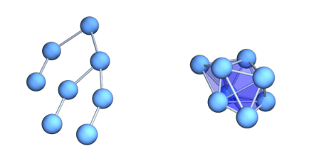
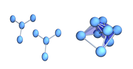
A graph without closed loops (including triangles) is also called a forest. The connected components of a forest are trees. This includes one point graphs which can be considered seeds of a tree. Forests are triangle free graphs and so have maximal dimension . Forests which do not consist entirely of seeds define simplicial complexes for which the Euler characteristic is equal to the number of trees. This is a consequence of the Euler-Poincaré formula and the fact that the contractibility of each component implies all Betti numbers to be zero for positive and especially the genus . One can also prove this by induction by seeing that adding branches to a tree does not change the Euler characteristic: any growth of the tree adds the same number of vertices and edges. Given a graph , one can look at spanning trees, trees within which have the same number of vertices or spanning forests. A rooted tree assigns to a tree also a base point, the root.
4.3.
Trees and forests in general are important structures in graph theory. The matrix tree theorem tells that the number of rooted spanning trees in a graph is the pseudo determinant (the product of the non-zero eigenvalues of ), of the Kirchhoff Laplacian of the graph. And is the number of rooted forests in the graph. The number of trees is then , where is the number of vertices. And the number of forests is . This is the matrix forest theorem of Chebotarev and Shamis [79]. Both the tree and forest results readily follow from a generalized Cauchy-Binet result. (See [35, 30] for some results and references.)
4.4.
The number of spanning trees of a graph is also called the tree complexity while the number of rooted spanning forests divided by is the forest complexity. In the ratio of the complexities the disappears and leads to the quantity
is interesting. The tree and forest numbers grow exponentially fast but the ration of their complexities has a chance to go to a limit. Let denote the number of rooted trees and the number of rooted forests in .
| n | Tree | Forest | Tree | Forest |
|---|---|---|---|---|
4.5.
The tree-forest complexity ratio of rooted forest and rooted
converges. This is the fraction of the pseudo determinant over the Fredholm determinant of the Kirchhoff matrix of the graph. In terms of eigenvalues, it is
Because the eigenvalues different from and are explicitly known
which is the same list than
we have
The next formula also will allow to study tree-forest ratios for manifolds, where we do not have a finite amount of trees or manifolds to count. For , where is the Riemann zeta function, we have , more generally if is the diameter of the circle.
Lemma 2.
The forest-tree ratio is equal to
where is the spectral zeta function of .
Proof.
The forest-tree ratio of is
This product limit exists if the limits
etc exist and decrease because
∎
Theorem 5.
The forest-tree ratio of converges
where is the Euler number.
Proof.
The limit exists for all . It is for and else. Because is the complement of , the nonzero eigenvalues of the Kirchhoff matrix of can also be written as , where are the eigenvalues of . The spectrum therefore is in the interval . So, and for all . ∎
4.6.
The limit exists actually surprisingly often for graph complements of sparse graphs, where the complement has diameter . The limit is usually . This is very robust. Take for example a fixed finite set of generators in , then look at the circular graph , which is the Cayley graph. Now, the graph complement still satisfies
We can even increase the cardinality of the generators when taking the limit as long as goes to infinity. Of course, for cyclic graphs , the result is no more true. In general, if the graph diameter grows, also the tree-forest ratio grows simply because we have more possibilities to plant forests than trees. We will explore this a bit more elsewhere as it has relations with topological invariants.
4.7.
Given a forest , we can look at the graph complement . As is a rather sparse graph when seen as an embedding in a complete graph, the graph are quite messy in general. A bit surprising is that there is interesting topology coming in. A bit more surprising is that the topology can not be too complicated. In the following, we mean with “is a point” rephrasing that it is homotopic to a point and “is a sphere“ with is homotophic to a sphere”.
Corollary 3.
The graph complement of a tree is a point or a sphere, (meaning as usual that it is either contractible or homotopic to a sphere).
4.8.
The proof is has three ingredients:
(i) The graph complement of a disjoint union is a join and the
union of points and spheres produce a monoid under the join addition.
These statements are true for homotopy points and homotopy spheres.
The addition of a contractible graph and any other graph
is contractible (as one can see by induction in the number of points in .
We still have to see that if is a homotopy sphere and is a homotopy sphere,
then the joint is a homotopy sphere. We can see this also by induction.
A homotopy sphere is characterized as a graph which allows a contractible part to
be taken away obtaining a contractible graph. In other words, a homotopy sphere
is a graph which is the union of two contractible graphs and which is not contractible
by itself. In other words, a homotopy sphere is a graph of Lusternik-Schnirelman
category 2 and this property is preserved under the Zykov join operation.
(ii) For star graphs or linear graphs, the graph complements are either
spheres or points.
(iii) If a linear graph with endpoints (leaves) is added to an other graph connecting to a leaf of , then the same properties like for disjoint sums hold except that the graph can collapse a sphere to a contractible one and a contractible one to a sphere. In other words, the wedge sum of two trees when done along leaves produces on the graph complement the same effect (modulo homotopies) than the disjoint sum.
Corollary 4.
The graph complement of a triangle free graph is either a point, a sphere or a wedge sum of spheres.
4.9.
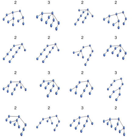
We just need to see when we add disconnected graphs together. Combining two one-dimensional graphs is done by the join followed by a removal of an edge. Both preserve the union of the set of contractible and sphere graphs. We so far have not yet been figured out which tree complements give spheres and which tree complements give contractible graphs. This is equivalent of knowing the cohomological dimension of a tree complement.
5. Morse build-up
5.1.
A sequence of graphs is a Morse filtration of if the subgraphs is obtained from by adding a vertex connected to either a contractible part of or to a subgraph which is homotopic to a -sphere. If is the numerical function on the vertex set of telling at which time the vertex has been added, then is the unit sphere and . We can then assign a Poincaré-Hopf index . Because -spheres have Euler characteristic , the indices on a graph with a Morse filtration are in .
Corollary 5.
The graphs admit a Morse filtration.
Proof.
This follows from the developments of the cohomologies and the fact that going from to produces a suspension. When we add a new vertex going from nothing changes, while going from either has index or . ∎
5.2.
Discrete Morse theory emerged in the 1990ies [10, 11]. A different take came from digital topology [16, 7]. But all this can be done conveniently also within pure graph theory. Topological features can now be observed in number theoretical contexts. In [46] we have looked at the graphs with vertex set and edges consisting of unordered pairs in , where either divides or divides . This produced a Morse filtration for . We had there with the Mertens function . The values of the Möbius function are Poincaré-Hopf indices of the counting function . This cell complex has been introduced already in [3].

5.3.
Every simplicial complex can be built up by starting adding vertices, then edges, then triangles etc until the entire complex is there. Each addition of a -simplex means to attach a -dimensional cell (handle) by attaching its boundary (a sphere) to the already given complex. More generally, with a notion of “sphere” as a complex which becomes contractible after removing a contractable part, we can define more general CW complexes in purely combinatorial manner. When attaching a new cell to a contractable part, we have a homotopy step.
5.4.
In the case of graphs, a Morse build-up is not always possible. In the cube graph for example, we can not remove any point because each point is attached to three vertices. In order to decompose the complex, we would have to treat it as a simplicial complex and remove edges first. The graphs are interesting graphs because we can build them up by adding vertices and so have a Morse build-up. What is remarkable that the Morse build-up is possible even with all stages to be spheres or wedge sums of spheres. Such deformations by adding points is certainly not possible for discrete manifolds. But here it is possible is a pentagon. It is deformed to which is which then is deformed to which is the Moebius strip and again .

5.5.
If is the linear graph with vertices obtained by snapping an edge from the cyclic graph , then its graph complement shall be denoted with because it is obtained from by adding an edge. The automorphism group of and so is , in comparison to the dihedral group symmetry which is the automorphism group of or .
Lemma 3.
The graphs contractible and are homotopic to -spheres. Two of the unit spheres of are , all other unit spheres are . All of the unit spheres of are .
5.6.
This means that we can build up as a Morse complex. One third of the time we have a homotopy extension, the other times, we alternating add even or odd dimensional cells. It follows that also is a Morse complex.
5.7.
We have seen that the unit spheres of are and that two unit spheres of are . Indeed we have
Corollary 6.
The intersection of two non-adjacent unit spheres in is . The intersection of two adjacent unit spheres in is .
6. Dimension
6.1.
The maximal dimension of a graph is one less than the clique number of and is the dimension of the largest complete subgraph which can occur in . The inductive dimension [24] of is the average over all dimensions of unit spheres. One has
with equality for discrete manifolds or complete graphs. The dimension expectation finally is defined as , the average simplex cardinality . We have proven the inequality
which is true for all graphs and sharp as we have equality for complete graphs [21]. Finally, we have the cohomology dimension which is defined in general as the largest for which the Betti number is non-zero. We also have
with equality for -sphere manifolds.
6.2.
Let us compute a few of these dimensions for the graph complements of the cyclic graphs .
6.3.
The average simplex cardinality is computable because are explicitly known hyper Fibonacci numbers and are multiples of standard Fibonacci numbers:
Lemma 4.
While is a hyper Fibonacci number, the derivative for is equal to , where is the ’th Fibonacci number. The average simplex cardinality therefore is
6.4.
Lets look at the dimensions for the graph complements of path graphs with vertices:
7. Cohomology
7.1.
One of our motivations to look at the graphs was to do use them for computations, like computing statistical properties or algebraic properties like cohomology groups and also higher order cohomology groups. This brings us often to the limit what a machine can do with current technology.
7.2.
When looking at the cohomology of , each Betti number stabilizes and eventually is zero except which remains always . Fr on, we have connected graphs , from on, we have simply connected graphs. From , on we have the second Betti number . When looking at the cohomology we noticed quickly that we have spaces homotopic to spheres or bouquets of two spheres. There is a “stable homotopy feature” in that modulo suspension we see a -periodicity: sphere-sphere-point-sphere-sphere-point etc.
7.3.
Here are the Euler characteristic and Betti numbers for the dual path graphs . There is again a -periodicity for the Euler characteristic and a -periodic pattern in the Betti number shift:
7.4.
On our off the shelve workstation, we were able to compute all the cohomology groups up to , where the simplicial complex of has simplices. We have then already to compute the kernel of matrices of this size. It is a computational challenge to go higher. Due to the cyclic symmetry, we know the nature of the harmonic forms in the sphere case. In the case of the wedge sum of spheres, the harmonic forms are more interesting. Since the kernel of an integer matrix always can be given by integer matrices, we could also wonder about the arithmetic of the individual entries of the harmonic forms. They are certainly of geometric interest
8. Wu characteristic
8.1.
We have seen . which is a 6 periodicity for Euler characteristic
summing over all complete subgraphs in , where with . There is now a 12 periodicity of the Wu characteristic
summing over all pairs of intersecting simplices in . Since , the notation is consistent. We see that the Wu characteristic is -periodic in . In the following table, we also compute the cubic Wu characteristic
which sums up all possible triple interactions. It is always equal to the Euler characteristic . The fourth order Wu characteristic
again agrees with .
8.2.
We believe that all agree and that all agree. This is a property which holds for discrete manifolds. In some sense, the graphs behave like manifolds or manifolds with boundary. In the case when is contractible which happens for , we deal with a manifold with boundary. In the other cases we have manifolds or a wedge product of manifolds .
8.3.
While Wu characteristic and its cohomology appear less regular [47] we again see a “stable homotopy” feature in that there is a -periodicity in which corresponds to a -periodicity in the cohomological dimension of . Here is the list for :
8.4.
We have computational power to compute the Wu Betti numbers of beyond yet, as the matrices get too large. The Wu Betti numbers behave already more erratic with respect to suspension. While the Betti vector just shifts , the Wu Betti numbers behave more interestingly. Examples of transitions under suspension are or .
8.5.
The f-matrix of a simplicial complex is counting the number of non-empty intersections of and dimensional simplices. Then
Lets denote with the f-matrix of . We have
In order to understand the periodicity of the Wu characteristic , we need to understand a recursion for the f-matrices . This needs still to be done. We see that each entry grows polynomially but we have still to understand the recursion. We have for example but already in the second row, we there are intersections possible which does not mean subsets.
9. Graph theory
9.1.
In this section, we collect now some graph theoretical notions of . They all pretty much follow from the definitions. The graphs have constant vertex degree and so in particular are all regular. Because are strongly regular (not only but for and for ), also are strongly regular. The graphs and are both claw free because they are graph complements of triangle free graphs. Bot and are connected and non-bipartite for . The graphs are also vertex transitive because the complement is. They are not edge transitive for . The graphs are never Eulerian as the vertex degrees are both or . The graphs Eulerian if and only is odd, by Euler-Hierholzer theorem which tells that even vertex degree everywhere is equivalent to the graph being Eulerian. The vertex degree of is which is the number of vertices in . The graphs are all Hamiltonian for all , and so are for . For even , the result for follows from the Nash-Williams theorem. Much simpler is just to write down a path: pick an integer with no common divisor with , then use the translation to get a closed Hamiltonian path . To compare, it is much harder to show that all combinatorial manifolds are Hamiltonian [53], a result which generalizes Whitney’s result for 2-spheres. A bridge-less graph (isthmus free graph) contains no graph bridges (edges which when removed make the graph disconnected). Here is a summary:
Theorem 6 (Graph properties).
The following properties hold:
- •
The graphs are strongly regular, and vertex transitive.
- •
The graphs are circulant graphs and for are biconnected and bridge-less.
- •
The graphs are connected for and disconnected for .
- •
The graphs are Hamiltonian for .
- •
The graphs are Eulerian, the graphs are not.
- •
The graphs and are always claw-free.
- •
The graphs are Cayley graphs of with two generators
- •
The graphs are the unit spheres of .
9.2.
The chromatic number of a graph in general is dual to the clique covering number. The independence number is dual to the clique number. The independence number of is because the clique number of is . The chromatic number of is , where denotes the integer part. In other words, the chromatic number of is . The independence number of is constant because the clique number of its graph complement is . The clique covering number is the chromatic number of which is equal to or depending on whether the graph is even or odd. Therefore, the graphs are perfect graphs while are not. The graphs are always perfect. By the perfect graph theorem is perfect if and only if is perfect. We know that are perfect while are not and that the path graph , the dual of is always perfect. The Shannon capacity of a graph is defined as , where is the ’th strong power of and the independence number. The Wiener index of a graph is where is the distance matrix. The graph distance matrix of is a circular matrix which has everywhere except in the side diagonal, where the value is and the diagonal, where the value is . The sum over all entries is therefore . The Harary index of a graph is . The Wiener and Harary indices are relevant for example in chemical graph theory [83]. The Harary index is for for for as can be seen by induction. Let us summarize these observations which all pretty much depend on the definitions:
Theorem 7 (Graph quantities).
The following quantities are known:
- •
The graphs have maximal dimension meaning clique number .
- •
The graphs have diameter for all .
- •
The Wiener index of is , for is , all for .
- •
The Harary index of is , for it is , all for .
- •
The graphs have maximal dimension , clique number .
- •
The graphs all have the independence number .
- •
The have chromatic number .
- •
The graphs have clique covering number , the graphs have clique covering number .
- •
The graphs are not perfect but all and all are perfect.
- •
The Shannon capacity of both and are always .
9.3.
When taking the strong product of cyclic graphs (introduce by Shannon in [81] in 1956 as the graph with Cartesian vertex set and edges which project on both factors to points or vertices), the clique number multiplies. It is under the large product (which is dual to the strong product) that we do no know what happens with the independence number. See [49, 51] for a bit more on the arithmetic of graphs. The large product of corresponds to the strong product of . While the Shannon capacity of is always , one only knows [75] among odd cyclic graphs and so far only has estimates for the Shannon capacity of . It is kind of funny that the Shannon capacity for cyclic graphs is a difficult vastly unsolved problem while the Shannon capacity for the dual graphs is easy. As complements of sparse graphs are pure communication error graphs. It is pretty much the worst case as independence number means that the graph is the dual of a graph with clique number and so must be a complete graph. Shannon capacity also characterizes complete graphs. Graphs with larger Shannon capacity have at least capacity . Already the cyclic graphs illustrate that the Shannon capacity computation for general circulant graphs is difficult in general.
9.4.
Lets look a bit about the metric space obtained by the geodesic shortest distance function as metric. Due to symmetry, the graph distance matrix of is a circulant matrix with in the side diagonal, in the diagonal and everywhere else. The diameter of is a consequence that two unit spheres always intersect for as there is then for any pair a third point such that the distances and are larger than so that are all connected in .
9.5.
If (which means that it is a -sphere), then the intersection is homotopic to a by -sphere or then is contractible. If (it is then a wedge sum ), then the intersection is either a -sphere, a -sphere or then contractible. If (which means it is a -sphere), then the intersection is either a sphere or contractible. What happens is that any intersection of unit spheres is always a smaller dimensional sphere or contractible. The Euler characteristic of any intersection of spheres in is always in . This property not only holds in . It also holds for Riemannian manifolds that are round spheres in Euclidean spaces or round spheres in Euclidean rotationally symmetric spheres. It also holds in homogeneous constant negative curvature manifolds. It fails in general for Riemannian manifolds, even flat ones like flat Clifford tori embedded in . So, the spaces behave very much like universal covers of Riemannian manifolds with constant sectional curvature. By the Killing-Hopf theorem, these are space forms, which are either spheres, Euclidean spaces or hyperbolic space. This will bring us to notions of curvature in the next section.
Theorem 8 (Space form property).
If are vertices in , then is the graph complement of a subgraph of in which the vertices are deleted. They are joins of spheres or contractible graphs and so themselves all either a sphere or contractible. The genus of is in .
Proof.
This is just obtained by seeing disjoint union into Zykov join in the graph complement. A unit sphere consists of all points in connected to . This means that the graph complement consists of all points in not connected to , meaning that has been taken off. More generally, the graph is the graph complement of in which the vertices are deleted. Under Zykov join the genus multiplies. Since spheres have genus in and contractible graphs have genus , we know the genus of all intersections of unit spheres. ∎
10. Differential geometry
10.1.
Differential geometric notions come in when looking at curvature in graph theory. In classical differential geometry, curvature is a rather technical notion involving the Riemann curvature tensor leading to the Gauss-Bonnet-Chern curvature which integrates on even dimensional manifolds to Euler characteristic. We have worked on this more recently [68, 69, 57] in the context of the open Hopf conjecture, a topic which also can be explored in the discrete. With a very strong sectional curvature assumption (all embedded wheel graphs have positive curvature), one gets spheres [63].
10.2.
In the discrete case, when looking at graphs, we have a much simpler task when looking at notions of curvature which add up to Euler characteristic. There are no technical assumption whatsoever necessary for an analogue of Gauss-Bonnet-Chern result and integral geometric considerations writing curvature as index expectation (which is possible both in the continuum as well as in the discrete) shows that the discrete case is the right analogue. We do not even have to worry about triangulations, as things are so robust. Take for example an dense set of points on the manifold then look at the intersection graph obtained by balls at these points. Averaging the discrete curvature over balls then produces the Gauss-Bonnet-Chern curvature in the limit. The graphs approximating are messy, have huge dimension but they are homotopic to for small enough and their unit spheres have diameter or and are either homotopy spheres or contractible. We pretty much have the frame-work we consider here in the case of .
10.3.
Lets look at the graphs now. The high symmetry given by a vertex transitive circle action produces a constant Euler-Levitt curvature
which is defined for all graphs and satisfies the Gauss-Bonnet relation . This curvature is always zero for odd-dimensional discrete manifolds because of Dehn-Sommerville. It is a discretization of the Gauss-Bonnet-Chern integrand for even-dimensional discrete manifold. One can see this by the fact that is the expectation of Poincaré-Hopf indices [25, 27] when averaging all locally injective functions and that the Gauss-Bonnet-Chern integrand of an even-dimensional manifold also is an average over Morse functions obtained by Nash embedding into an ambient Euclidean space and taking the Morse functions obtained by restricting linear functions on . This procedure can also be done on a graph with vertices. Embed it into then a random linear function in induces a coloring on the graph and so a Poincaré-Hopf index. The average is the Euler-Levitt curvature [74, 23] similarly as the Gauss-Bonnet-Chern curvature is the average over Morse indices.
Theorem 9.
While has constant curvature at every point, the graphs have nontrivial curvature distribution.
Proof.
The transitive automorphism group shows the constant curvature for . The curvature of is more interesting. It still adds up to of course. It can not be constant zero because some unit spheres are homotopic to spheres with positive Euler characteristic or contractible (with Euler characteristic ). ∎
10.4.
The curvatures of converge to something interesting. For example, for , we have the curvatures
The structure becomes only apparent however if one looks at large cases. The curvatures then converge to an attracting -period cycle.
10.5.
We see better what happens if we do not sort the curvature values. The next picture shows this:
10.6.
We have a convergence of curvature of in the limit because every unit sphere in is the join of two unit spheres of the form and so that we can give explicit formulas for the curvature. We can best formulate this using generating functions and using the functional Gauss-Bonnet theorem.
Theorem 10 (Curvature formula).
The curvature of at the vertex is
with .
Proof.
To compute the Euler-Levitt curvature at , we use the generating function at the vertex and get
The unit sphere of at is the dual graph of the disjoint union of two graphs and . In the graph complement, the disjoint union becomes the Zykov join. And for the Zykov join, the simplex generating functions multiply. ∎
10.7.
Now, for any fixed , the sequences
satisfies the same recursion. We also know from Gauss-Bonnet for that
10.8.
Using and and we get the explicit formula
We would still like to understand the limiting functions
10.9.
We see that we are able to compute the discrete analogue of the Gauss-Bonnet-Chern curvature for these high-dimensional spheres in a situation, where the curvature is not constant. Without this functional knowledge, computing the curvature directly is no more feasible already for numbers like where we deal with 12-dimensional spaces already. For , we have already simplices.
10.10.
While we see periodic attractor of a re-normalization map but we have not yet explicit expressions for the limiting attracting curvature functions. Similarly as in [40, 43] we get to a result which can be seen as a central limit theorem for Barycentric subdivision. Unlike in the cases studied, we do not look at the spectral distribution (the result there applies also here of course) but at the Euler-Levitt curvature distribution of graph complements of linear graphs in the Barycentric limit. The curvature distribution of the graph complements of of course is trivial because all unit spheres there are the isomorphic graphs.
11. Renormalization
11.1.
We have seen that for the one-dimensional interval when discretized as a linear graph , the graph complement is either a point or sphere. Let be the renormalization map, then has length and has vertices. Then is always a -sphere, where or .
11.2.
Lets look at examples with small . The graph complement of and the graph complement of is the house graph and so a -sphere, the path graph of length is a -sphere, the graph complement of the path graph of length is a -sphere and the graph complement of of length is already a sphere. For even we get odd dimensional spheres for odd we get even dimensional spheres .
11.3.
The discrete Euler curvatures of the graph complement can be attached to the vertices of and can be computed directly. This curvature is
with satisfying the recursion
While
does converge weakly to the Lebesgue measure along even subsequences and to along odd sub-sequences. But if we split it up, we see more structure.
11.4.
Define the functions on as
11.5.
If we do Barycentric refinements, then and we always have spheres. It is remarkable that we have now smooth non-trivial renormalization curvature limits. For each , there are three non-trivial functions which together add up to a constant function
These curvatures build up Gauss-Bonnet curvatures onthese large dimensional spheres.
Theorem 11 (Renormalization limit).
The curvature function limits exist on for .
Proof.
(Sketch) The explicit formula
with are integrals of polynomials in . These hyper-geometric functions can be written as sums of line integrals from to one of the ’the roots of unity. The fact that terms of the form and appear show that the limit is periodic in for any choice of . ∎
11.6.
We see that the limits are smooth functions and expect to prove this from explicit formulas for the limiting function. The curvature expressions are given by explicit hyper-geometric functions which are integrals of polynomials in .
11.7.
When looking at the story from the renormalization perspective, where we do Barycentric refinement , we can also generalize this to higher dimensions and make Barycentric refinements of higher dimensional graphs. This is very difficult to investigate numerically because things explode very fast. To illustrate this, take the complete graph which is a triangle. The graph complement is the three point graph without edges and Betti vector . The graph complement of the Barycentric refinement of has the -vector and Betti vector . The second Barycentric refinement of has as a graph complement a graph with f-vector which means a total of 16886 simplices. The Betti vector is . According to Euler-Poincaré, the super sum of both the Betti vector and the f-vector is the same. It is 22. We were unable to compute both the -vector and the Betti vector of the graph complement of the third Barycentric refinement.


12. Fixed point theory
12.1.
Since has a dihedral group symmetry generated by a translations and reflections . We can now look at the Lefschetz number of an automorphism . It is defined the super trace
of the induced action of on the cohomology groups which is by Hodge just the null space of the Hodge operator restricted to the -dimensional block of -forms.
12.2.
A special case is when is the identity map. The Lefschetz number is now which is the Euler characteristic. The Lefschetz fixed point theorem now becomes a special case, the discrete Euler-Poincaré theorem [5, 6]. In the case of the circular graphs, we have the Lefschetz number and consequently no fixed points. We can compute the Lefschetz number by looking at the fixed point and use the Lefschetz fixed point theorem [29]
where is the Lefschetz index.
12.3.
The Lefschetz numbers are defined for every . The average
can be interpreted as the Euler characteristic of the chain . (The simplest way to do that is to define the Euler characteristic of as such). The prototype example is , which has the same automorphism group like and where the Lefschetz number is zero for every translation but equal to for every reflection. The average Lefschetz number is then always . If we take only the subgroup of orientation preserving maps, then the chain has Euler characteristic which is indeed . If we factor out the dihedral group then and can be seen as a point.
12.4.
In our case, the Lefschetz numbers can not be too complicated because the cohomology groups are not. In the case when we have not divisible by , we deal with spheres and the Lefschetz number can only be in depending on whether the map switches the sign of the Harmonic -form (in the sphere case, the harmonic forms form a one dimensional space only). In the case , we can have Lefeschetz numbers in as we have harmonic -forms. The maximum is obtained if does not flip the sign of both forms. The minimum is obtained when switches both signs. Here is a computation of the Lefschetz numbers for all automorphisms of for small . We see the structure. For all cases where is homotopic to , all Lefschetz numbers zero. For even , the Lefschetz number of reflections are either or while for , the Lefschetz number of any reflection is . The story clearly only depends on whether is even or odd and what happens modulo for .
Theorem 12.
The possible Lefschetz numbers show a -periodic pattern. The average Lefschetz number is except for the cases and where the average Lefschetz number is .
The program computing these numbers by finding all fixed points and then adding up the Lefschetz indices is given below. We could push the computation to but needed to add graph specific code to find all the simplices in the graphs. Clique finding for graphs is already hard. Fortunately, there is a recursive way to generate all complete subgraphs of .
| n | Rotations | Reflections | average |
|---|---|---|---|
| 4 | (0,2,0,2) | (2,0,2,0) | 1 |
| 5 | (0,0,0,0,0) | (2,2,2,2,2) | 1 |
| 6 | (0,2,3,2,0,-1) | (1,1,1,1,1,1) | 1 |
| 7 | (0,0,0,0,0,0,0) | (2,2,2,2,2,2,2) | 1 |
| 8 | (0,2,0,2,0,2,0,2) | (0,2,0,2,0,2,0,2) | 1 |
| 9 | (0,0,3,0,0,3,0,0,3) | (1,1,1,1,1,1,1,1,1) | 1 |
| 10 | (0,2,0,2,0,2,0,2,0,2) | (0,2,0,2,0,2,0,2,0,2) | 1 |
| 11 | (0,0,0,0,0,0,0,0,0,0,0) | (0,0,0,0,0,0,0,0,0,0,0) | 0 |
| 12 | (0,2,3,2,0,-1,0,2,3,2,0,-1) | (1,1,1,1,1,1,1,1,1,1,1,1) | 1 |
| 13 | (0,0,0,0,0,0,0,0,0,0,0,0,0) | (0,0,0,0,0,0,0,0,0,0,0,0,0) | 0 |
| 14 | (0,2,0,2,0,2,0,2,0,2,0,2,0,2) | (2,0,2,0,2,0,2,0,2,0,2,0,2,0) | 1 |
| 15 | (0,0,3,0,0,3,0,0,3,0,0,3,0,0,3) | (1,1,1,1,1,1,1,1,1,1,1,1,1,1,1) | 1 |
| 16 | (0,2,0,2,0,2,0,2,0,2,0,2,0,2,0,2) | (2,0,2,0,2,0,2,0,2,0,2,0,2,0,2,0) | 1 |
| 17 | (0,0,0,0,0,0,0,0,0,0,0,0,0,0,0,0,0) | (2,2,2,2,2,2,2,2,2,2,2,2,2,2,2,2,2) | 1 |
| 18 | (0,2,3,2,0,-1,0,2,3,2,0,-1,0,2,3,2,0,-1) | (1,1,1,1,1,1,1,1,1,1,1,1,1,1,1,1,1,1) | 1 |
| 19 | (0,0,0,0,0,0,0,0,0,0,0,0,0,0,0,0,0,0,0) | (2,2,2,2,2,2,2,2,2,2,2,2,2,2,2,2,2,2,2) | 1 |
| 20 | (0,2,0,2,0,2,0,2,0,2,0,2,0,2,0,2,0,2,0,2) | (0,2,0,2,0,2,0,2,0,2,0,2,0,2,0,2,0,2,0,2) | 1 |
| 21 | (0,0,3,0,0,3,0,0,3,0,0,3,0,0,3,0,0,3,0,0,3) | (1,1,1,1,1,1,1,1,1,1,1,1,1,1,1,1,1,1,1,1,1) | 1 |
| 22 | (0,2,0,2,0,2,0,2,0,2,0,2,0,2,0,2,0,2,0,2,0,2) | (0,2,0,2,0,2,0,2,0,2,0,2,0,2,0,2,0,2,0,2,0,2) | 1 |
| 23 | (0,0,0,0,0,0,0,0,0,0,0,0,0,0,0,0,0,0,0,0,0,0,0) | (0,0,0,0,0,0,0,0,0,0,0,0,0,0,0,0,0,0,0,0,0,0,0) | 0 |
| 24 | (0,2,3,2,0,-1,0,2,3,2,0,-1,0,2,3,2,0,-1,0,2,3,2,0,-1) | (1,1,1,1,1,1,1,1,1,1,1,1,1,1,1,1,1,1,1,1,1,1,1,1) | 1 |
12.5.
And here are the Lefschetz numbers of all automorphisms of for small . The graph has the same automorphism group than the linear graph with vertices. There is no translation any more.
| n | Lefschetz of | average |
|---|---|---|
| 4 | (1 , 1) | 1 |
| 5 | (0 , 2) | 1 |
| 6 | (0 , 2) | 1 |
| 7 | (1 , 1) | 1 |
| 8 | (2 , 2) | 2 |
| 9 | (2 , 0) | 1 |
| 10 | (1 , 1) | 1 |
| 11 | (0 , 0) | 0 |
| 12 | (0 , 0) | 0 |
| 13 | (1 , 1) | 1 |
| 14 | (2 , 0) | 1 |
| 15 | (2 , 2) | 2 |
| 16 | (1 , 1) | 1 |
| 17 | (0 , 2) | 1 |
| 18 | (0 , 2) | 1 |
13. Code
13.1.
The following code generates the basis for all the cohomology groups of a simplicial complex (a finite set of sets closed under the operation of taking finite non-empty subsets). The Wolfram language serves well also as pseudo code. Since no libraries are used, it should be straightforward to rewrite the code in any other programming language. The programs can be accessed from the LaTeX source of the ArXiv submission. We give it here for the situation at hand. We first generate the complex for the graph . Then we compute the Betti vector. The last line in the following block finally prints the spectral picture of the Hodge operator. We always start with a clean slate, clearing all variables.
13.2.
And here is the code producing the connection cohomology groups which are more subtle and no more homotopy invariants. The following lines are independent of the above for the sake of clarity. It computes the Wu cohomology of the Moebius strip which is remarkably trivial. Having all cohomology groups trivial is not possible for simplicial cohomology.
13.3.
Here are the lines to compute the curvature of a complex. It works for arbitrary simplicial complexes and is done in a functional way. For more details, see [59]. What is new here is that we work directly with simplicial complexes and do need to generate Whitney complexes of unit sphere graphs. The unit sphere in a complex is now a set of sets and not a simplicial complex but still has a simplex generating function , where is the length of . Gauss-Bonnet is then a theorem about generating functions and tells for the simplex generating function of :
where is the anti-derivative and are the zero-dimensional parts of . The curvature at a vertex is then a function too . This functional generalization works also for Poincaré-Hopf [20].
13.4.
Because of the explicit formulas, we have a faster way to get the curvatures if we deal with . This is the curvature formula. The following code also is completely independent from any thing before. We then plot the list which produces the shape of the limiting functions
13.5.
Here are the lines to compute the Lefschetz numbers of . Also this code is independent from anything before in order to make it easier to port it to other programming languages. The Wolfram language is perfect for pseudo code but requires quite a bit of memory. We can not compute yet all the Lefschetz numbers for for example. The task is simple: make a list of fixed point simplices and add up the indices to get the Lefschetz number using the discrete Lefschetz fixed point theorem. In the following code, we have a custom fast computation of the Whitney copmlex of . We know from the recursion that it can be obtained by using the Whitney complexes of and and add a point to . What we essentially do when computing the Whitney complex of is compute all possible king configurations on a one-dimensional chess board of length . On board of length for example there are possible king configurations.
13.6.
And here is the computation of the limiting Euler curvatures of the graph complements of length (point) , (odd sphere), (odd sphere), (point) , (even sphere), (even sphere). In each case, the averaged curvature is constant whereas in reality, there are three separate parts of the graph in which the curvature function is different. This is a case, where we see much more structure than in the continuum: now, the curvature at a node depends on the number theoretical modulo 3 case and the nature of the geometry changes in a 6 periodic manner. We first compute the generating functions starting from so that is the third element. Then we compute the curvature at the node as and then get the limiting curvature functions
for in each of the cases .
13.7.
This separation of the curvature parts explains the discontinuous curvature distribution function obtained by just plotting an ordered list of curvatures of the graph complements. These curvature distribution functions converge in the limit . Who would think that a one dimensional path has such an interesting dual.
13.8.
Here is the code for computing the tree-forest ratio which the ratio between the Fredholm and Pseudo determinant of the Kichhhoff matrix. We also give the expression when taking the explicitly known eigenvalues. See [35] for more details on trees and forests and Cauchy-Binet.
14. Miscellanea
14.1.
In this quite inhomogeneous section, we collect a few mathematical parts and lose ends. It is presented a bit differently and in parts slightly more general than in previous attempts of talks [31, 36, 52] as some of the things have evolved a bit. We especially review the various generalizations of Gauss-Bonnet, Poincaré-Hopf or Lefschetz by either looking at valuations (energizations of the graph with some symmetry), or functionals (like simplex generating functions). Curvature becomes elegant in the functional frame work. Of course, all this needs to be organized once in a single monograph; at the moment however we are much more interested in experiments, finding new patterns and relations, rather than working on consolidation.
14.2.
Graphs and complexes. A finite simple graph is equipped with its Whitney complex, the simplicial complex consisting of the vertex sets of all complete subgraphs. Not all finite abstract simplicial complexes are Whitney complexes of finite simple graphs. An example is which is the -skeleton of the -dimensional complex . The Barycentric refinement of a complex is the order complex of consisting of all non-empty subsets of which are pairwise contained in each other. The refinement is the Whitney complex of the graph in which the vertices are the elements of and two are connected if one is contained in the other. We see that graph theory very well captures most interesting simplicial complexes.
14.3.
Homotopy. The notion of homotopy is based on the notion of contractibility which is inductively defined. A homotopy extension of a finite simple graph chooses a contractible subgraph in , adds a new vertex and adds all connections from to all . The reverse operation is a homotopy reduction. It picks a vertex for which the unit sphere is contractible and removes this vertex. Two graphs are homotopic if there exists a finite set of homotopy extension or homotopy reduction steps which brings to . Being homotopic to a point is difficult to check in general while contractibility, meaning that can be reduced to a point (without any extensions) can be done fast. The properties of graph homotopy are identical to the properties for classical homotopy deformations of nice topological spaces like CW complexes. One could use the geometric realizations of with Whitney complex to prove these things but all the mathematics can be done within combinatorics, meaning for example not having to use the infinity axiom. The valuation property for Euler characteristic immediately shows that an extension changes Euler characteristic by adding . This is zero for homotopy extensions as then. Simplicial cohomology remains the same under homotopy deformation: any cocycle on can modulo coboundaries on become a cocycle on . The homotopy on graphs produces a chain homotopy for the differential complex. Natural operations like edge refinements or Barycentric refinements are homotopies. The Wu cohomology however is not a homotopy invariant: for example, . The graph has all cohomology groups zero while the discrete cylinder has also non-zero Wu cohomology groups.
14.4.
Differential geometry. The -vector of a finite set of sets encodes the number of -dimensional sets in . The simplex generating function abbreviated as -function is defined as . Its anti-derivative is the curvature function. Let the set of -dimensional sets in , the sets of cardinality . It is also called the vertex set of the complex and if is the Whitney complex of a graph , then the vertex set is . When pushing the values from simplices equally to all vertices contained in , we get the Levitt curvature. This can now be formulated as a Gauss-Bonnet result [59]:
Theorem 13 (Gauss-Bonnet).
, with curvature .
14.5.
For , this gives the Gauss-Bonnet formula [23]. For graphs, this gives the Euler-Levitt curvature . In the special case when the graph has circular unit spheres at every point it reduces to the famous which has first been considered [1] in the context of the 4-color theorem. In the case of triangle free graphs, where Gauss-Bonnet becomes the Handshake formula , the number of edges as is then the Euler characteristic. The general Gauss-Bonnet formula corresponds to the Gauss-Bonnet-Chern formula for even dimensional compact Riemannian manifolds but does not require any assumptions on the graph. We get the curvature distribution of random networks for example if we know the distribution of the observables . We have in [22] seen that for random Erdös-Renyi graphs with edge probability , the expectation giving the formula
which allows to see for example that in exponentially large positive or very negative Euler characteristic is possible. If we assume that the unit spheres of a graph have unit spheres which have a known distribution, we would also get a curvature expectation .
14.6.
There are topological approaches to graph coloring [37, 41] builds on work of Fisk [8, 9]. For maximal planar 4-connected graphs, which are by a theorem of Whitney always 2-spheres (graphs for which every unit sphere is a circular graph and which when punctured becomes contractible), the total curvature is and the chromatic number or . In general, the chromatic number of a d-sphere is believed to be or the reason being that one write as a boundary of a ball then use edge refinements in the interior to make the interior Eulerian so that it can be colored with the minimal amount of colors. This then colors the boundary. Now, in our case we have spheres which are not discrete manifolds and have very small diameter . The chromatic number is which grows faster than the dimension . we need colors to color while a discrete manifold sphere needs . A 3-sphere should have chromatic number 5, while our 3-sphere has chromatic number . The join for example which is a -sphere with -function and Euler characteristic has chromatic number . The Eulerian graph (see [42, 55] for the Eulerian theme) has minimal chromatic number (discrete 3-manifolds always have chromatic number at least 4 because of the existence of 3-simplices with 4 vertices).
14.7.
Gauss-Bonnet can be generalized to valuations for subgraphs of which in the case is Euler characteristic. The theory of discrete valuations [19] is a combinatorial theory of valuations developed by Hadwiger and others which is now part of integral geometry or geometric probability theory. While in the continuum, one requires some structure for the theory to work (like convex sets), the discrete works for all graphs. We have to do some Buffon type gymnastics in the continuum which allows to measure dimensional content in a dimensional manifold for example (like the length of a surface for example, which is approached by cutting it with random planes and measuring the length) while in the discrete we just count .
14.8.
An even more general set-up, is a energized complex , where is any ring. This is a frame work which appears quite often also in graph theory, like when looking at weighted graphs or when using orthogonal graph presentations like the Lovasz umbrella which allows to get upper bounds for the Shannon capacity of a graph. The generality of assigning rather general data to any part of a simplical complex does not prevent to look at notions of c9urvature. Define for the curvature which means distributing the energy of equally to all zero-dimensional parts in . The Gauss-Bonnet formula is too obvious as moving the energy from a simplex equally to each of its zero dimensional parts of course does not change the energy. Adding up all the energies of all the contributing simplices at a vertex is then the curvature. This can be done also by using other distributions, the extreme case being when distributing the energy to a minimum of some ordering, like for example given by a scalar function on the vertices. This is then Poincaré-Hopf.
14.9.
Even more general is to generalize this to multi-linear valuations like Wu characteristic where is the number of pairs of simplices and simplices in which have non-empty intersection. One can then even look at even more generality and see as a self interaction generalizing a more general interaction part
where is the number of pairs of simplices in and in which intersect. It even generalizes further by not insisting on having the same “energy” value for every -simplex. See [60, 65, 67]. For all these notions there is a Gauss-Bonnet relation. For example, for the Wu characteristic
one has the curvature , where is the simplex curvature . We have seen earlier [44] that the Wu curvature is the same than the Euler characteristic curvature if is a discrete manifold. The Wu curvature is
Theorem 14 (Wu Gauss-Bonnet).
.
14.10.
Since we have a -periodicity in the Wu-characteristic, we expect a 12-periodic fixed cycle for the Wu curvature. Since we have no recursion yet for the f-matrix of , we can not compute the curvature yet for larger .
14.11.
Poincaré-Hopf angle. If is a function which is locally injective in that if or , then it defines an total order the -dimensional parts on every simplex with if . This defines a map . Given a function . we can send to the largest element in . All these values add together to the Poincaré-Hopf index . We have now a Poincaré-Hopf theorem for gradient vector fields again formulated for simplex generating functions . Let be the part of the unit sphere .
Theorem 15 (Poincaré=Hopf).
.
A special case is if is the Whitney complex of a graph and is a locally injective function. Then See [25, 61, 20]. Also this idea can be generalized to multi-linear valuations [44] and there is a link to Gauss-Bonnet. Gauss-Bonnet can be seen as an expectation of Poincar e-Hopf [27] when averaging over a probability space of functions like for example averaging over all coloring functions with a minimal amount of colors [38].
14.12.
Brouwer-Lefschetz angle. We have illustrated above the Brouwer-Lefschetz theme and seen how it relates with cohomology. If is a simplicial complex, and is an automorphism of , then we have also an induced map on cohomology. The Lefschetz number is defined as the super trace of on cohomology. Let denote the linear space of harmonic -forms n and the induced map on , then
By Euler-Poincaré, we have .
14.13.
The fixed point set consists of all simplices which are fixed by . The index of a fixed point is where the sign of on is the sign of the permutation induced on the finite set .
Theorem 16 (Brouwer Lefschetz).
The proof is in [29]. As pointed out in the introduction the simplest way to prove this is by applying a heat flow and use the McKean-Singer super symmetry [28] which tells that the set of non-zero eigenvalues on even-dimensional forms is the set of non-zero eigenvalues on odd-dimensional forms implying for all positive powers . The McKean-Singer formula for the Hodge Laplacian tells then
Theorem 17 (McKean Singer).
.
One can see this by taking the Dirac operator serious and use the analogous proof in the continuum [4]. It maps even forms to odd forms and vice versa.
14.14.
There is also a Lefschetz fixed point story for Wu characteristic. But the computation is harder and the Lefschetz numbers are richer because the cohomology is richer. What happens is that the super trace of an automorphism induced on Wu cohomology is the sum of the indices of the intersecting fixed point pairs with respect to . Let us denote the Wu Lefschetz number of with . Then
Theorem 18 (Wu Lefschetz).
For example, in the case , the Wu Lefschetz numbers are given by the 12 numbers
belonging to the automorphisms of . The Wu-Betti vector is here . For , all Lefschetz numbers are zero simply because the cohomology is trivial.
14.15.
We have pointed out in [48] that whenever we have a McKean-Singer symmetry given by a symmetry Dirac operator then there is both an Atiyah-Singer type result (which is Gauss-Bonnet like) as well as an Atiyah-Bott type result (which is Lefschetz-Brouwer) like). Wu characteristic and its cohomology are examples for such a general view. Other examples are obtained by Lax deforming the matrix using an isospectral flow [33]. In any of theses cases, the heat flow for the operator produces the proof. Euler-Poincaré for Euler characteristic or Wu characteristic is the special case for the identity transformation . Despite the simplicity of the set-up, we still do not understand well the Wu characteristic cohomology as well as the Lefschetz numbers there. We also do not know the periodicity yet for the Lefschetz story for quadratic simplicial cohomology. On can wonder whether there is a relation with other periodicity results known in stable homotopy theory. It is not so far fetched as the homotopy theory of orthogonal groups is closely related to the homotopy theory of spheres and in our case, we have spheres realized with a group structure which in principle could be used to act on other spheres.
14.16.
Hodge spectrum. When computing the spectrum of the Hodge Laplacian of the graphs for large , we see that the spectrum appears to converge to a nice smooth function for . We have investigated the same problem in the case of and there convergence as a consequence of a general central limit theorem where because of Fourier theory one has explicit eigenvalues both for forms and -forms. The spectrum of the -forms converges so, but in the limit of larger and larger dimensional spheres, this becomes less and less visible. The McKean super symmetry used in 1 dimensions shows that the -dimensional non-zero spectrum is the same than the -dimensional non-zero spectrum. The number of zero eigenvalues of is then the number of components and the number of zero eigenvalues of is the genus , the number of “loops”.
14.17.
Now, for the graphs , we see again convergence of the spectrum when rescaled properly, but the method used in the case of Barycentric refinements does not apply because now. The dimensions of the simplicial complexes increases in . In the Barycentric refinement, we had convergence of the spectral density of states on every sector of -forms. [40, 43]. There are more open questions which are spectral. Unrelated one can also ask what happens with the spectrum of the connection Laplacians of . We measured until that the connection graphs of have the same cohomology than
14.18.
Let us come back to the spectrum of the Hodge Laplacian of the graphs . Two blocks of the Hodge Laplacian are well known: the Kirchhoff Laplacian as well as the highest block are circulant matrices allowing Fourier theory to compute the eigenvalues. This works for -forms: in a Fourier basis, the eigenvalues of the Kirchhoff matrix of are explicitly given as
We have .

14.19.
Zeta function aspect. Th zeta function theme related to spectral questions. It relates to harmonic analysis and complex analysis because we deal with analytic functions. Given a matrix with non-negative spectrum, one can associate a Zeta function with the non-zero spectrum. In the case of the Hodge Laplacian we have to discard the zero spectrum which is associated to cohomology. The zeta function is
Already in the case of the circle , where the Dirac operator has spectrum with and the Laplacian has eigenvalues , we have to discard the eigenvalue and take the square to get non-negative eigenvalues. It is custom to replace with to get then the Riemann zeta function . For counting Laplacians or for connection Laplacians of one-dimensional complexes, we know that the zeta function satisfies a functional equation. We would like to understand of course the Zeta functions in the Barycentric limits. This has been explored so far only for complexes coming from cycle graphs.


14.20.
14.21.
Here are again two main questions related to Wu characteristic and the spectrum. What happens with the Wu characteristic and Wu cohomology of ? We also do not know why the normalized spectrum of the Hodge Laplacian converges and why the curvature function of has a normalized limit. The Hodge Laplacian in full generality satisfies the McKean-Singer super symmetry [76] also in the discrete as we had pointed out in [28] and this also applies here. This symmetry implies that if there is a limiting density of states of the spectrum for the Laplacian, then it is the same when restricted to even or odd dimensional discrete differential forms.
14.22.
Connection aspect.
When looking not at incidences but intersections, some connection
linear algebra comes in. Since connection Laplacians are always invertible
we do not have to throw away the zero eigenvalue. See [45, 58, 60, 65, 67].
Connection Laplacians of complexes encode in their spectrum
a lot of topological information even so we do not know all yet.
The number of negative eigenvalues is the number of odd dimensional
simplices in the complex.
14.23.
The connection matrix of a simplicial complex is the matrix if
intersect and else. The determinant depends on the number of odd
dimensional simplices in . We have if
and equal to else. We also have for and
else. The number of positive eigenvalues minus the number of negative eigenvalues
of is the Euler characteristic [50]. As for the
counting matrix [58], where counts the number of simplices in
we have positive definite quadratic forms which are isospectral to
the inverse matrix which is also a positive definite quadratic form.


The Hodge Laplacian and the connection Laplacian are not always unrelated. in [56] we pointed out that for 1-dimensional simplicial complexes, the hydrogen identity holds, where is the sign-less Hodge Laplacian defined by the sign-less incidence matrix and where is the connection Laplacian. This is useful for estimating the Laplacian spectral radius .
14.24.
Many classical theorems in mathematics have discrete analogues which are technically much simpler. There are already versions of Riemann-Roch available. We tried once to see how a discrete Atiyah-Singer theorem would look like [48] by using the McKean-Singer spectral symmetry as an analogue replacing technical assumptions like elliptic regularity. The reason is that McKean-Singer spectral symmetry is really what one needs for having a notion of analytic index. Atiyah-Singer generalizes Gauss-Bonnet, Athiah-Bott generalizes Brouwer-Lefschetz. An example of such an “elliptic complex” is the Wu cohomology for Wu characteristic
for a finite abstract simplicial complex, where and means that the intersection is not empty. Wu characteristic is one of many multi-linear valuations [44]. Multi-linear valuations, like valuations have a homogenity condition in that the values for isomorphic graphs is the same. This allows to define the valuation by giving the value on -dimensional simplex tuples. In the case of generalized Wu characteristic, one has the value for intersecting tuples of simplices. This can be vastly generalized by looking more generally at a function [65, 60], where is a ring (this is a frame work which sometimes is also considered in frame works like interaction models [2]).
14.25.
Statistical aspect.
Statistical questions come in when asking what happens typically?
In our case, we can look what typical Euler characteristic, dimension, or simplex
cardinality we get for the graph complement of
a one dimensional graph with nodes. We would like to know what Betti numbers
can occur or what Betti numbers occur most likely. What Euler characteristic
what dimension appears typically [22]? What size of the simplices
[21].
14.26.
Then there is the geometric probability or integral geometric aspect, where one averages over probability spaces of external quantities. One can see curvature as an expectation of indices [27, 38, 26]. We see for example that the graph complements of most trees appear to be contractible (their cohomological dimension is ). The cases where we have spheres is less frequent and one could suspect that in the limit the probability of getting contractible graph complements is one.
14.27.
Dynamical aspect. There is a dynamical theme. What happens with quantum mechanical evolutions or isospectral deformations on a graph. See [33, 32]. While these features work for any graph, the dynamics could become more interesting in special cases like for example when we deal with graph complements of cyclic graphs.
14.28.
Dynamics also comes in when looking at automorphisms. This is especially interesting if is a Cayley graph of a group . We have seen the case of a Cayley graph with the group , where we take the complement of the natural generators and . An other example is the dihedral group the symmetry group of the -gon which is non-abelian. We looked at the topology of the complement graphs of the natural Cayley graphs. For , we look at the complement graph of the cube graph. Let us call these graphs. There seems to be a parallel story in that now these graphs are homotopic to either spheres or wedge products of 3 spheres. The later happens for .


| for n= | ||
|---|---|---|
In the dihedral case, where we look at the graph complements of the Cayley graph of dihedral groups, the computation of the f-function is also recursive but a bit more complicated:
14.29.
Positive curvature aspect A complete classification of positive curvature manifolds is still missing. All known cases admit a effective continuous group of effective symmetries. Such a symmetry must be a Lie group [72]. A reduction theory sees the fixed point manifold of this group action is a union of smooth positive curvature manifolds, where each has even co-dimension. All known positive curvature manifolds admit a circle action. Circulant graphs come already with a symmetry and it is natural to try to use them for constructing positive curvature manifold. There are some interesting consequences coming directly from the reduction. See [71] on a theorem of Grove and Searle [14] and references.
14.30.
What other manifolds can be obtained like this? For the graphs one can not identify points to get from to . However, one can look at Barycentric refinements and then take the quotient. One gets so discrete geometries for which one has a circular symmetry but the Euler curvature must be averaged to become positive. Barycentric refinements in general already introduce negative curvature. The Barycentric refinement of an icosahedron graph for example has curvature at some points of vertex degree . The curvatures still add up to 2. After an identification of a polar map one can get models of the projective plane and now the curvatures add up to . In the spirit of what we have done here, it is natural to look for larger classes of models and circulant graphs are natural.
14.31.
The quest to push computation of cohomology groups further is also motivated by the story of positive curvature. We would like to understand the cohomology of positive curvature manifolds better because we have a strange (possibly only mathematical) affinity between positive curvature manifolds and Bosonic matter in physics [70]. The heavy bosons are related to positive curvature manifolds which have more elaborate cohomologies.

14.32.
Number theoretical aspects. The are many questions open like how many fixed points the automorphisms of have of each dimension, then about the factorization of the polynomials . We see that always have a factor which indicates to be a suspension. But it is not necessarily. For where we get an f-function which is the same than of the join of . We also see experimentally that we can always modify the largest power of by adding with so that we have a factorization and that this is -periodic.
14.33.
A class of circulant graphs that is interesting in number theory is are quadratic residue graphs or Paley graphs defined by a prime power with . Paley graphs are self-complementary. The edges are all pairs such that is a square (a quadratic residue). For one has the squares so that we have . The next one is which is actually a 2-dimensional torus and a 2-graph. For -graphs, the curvature has been been defined already early in graph theory in the context of graph coloring and is . The Paley graph is remarkable as it is a discrete analogue of the Clifford torus. It is flat. The curvature is constant everywhere. For the next ones we always see constant curvature and . But then has constant curvature , is not geometric because the unit spheres have and constant curvature and Betti vectors .

14.34.
A natural question is to look for graphs which are d-manifolds in the sense that all unit spheres 22 2 The term “neighborhood” in graph theory is misleading as it suggests the midpoint to be included if the graph is a metric space. We would call the later a unit ball. Unit balls as pyramid extensions of unit spheres are always contractible. are spheres, where -spheres are -manifolds with the property that removing a vertex produces a contractible graph. This is a notion which agrees with other notions of spheres like in discrete Morse theory [62]. So far, only have turned out to be manifolds. Also the Lefschetz story needs more investigations. In the torus case each of the 13 involutions in the automorphism group all have Lefschetz number while all 13 translations in have . The average Lefschetz number is therefore in this case. In the cyclic case , we have like in all cases the average Lefschetz number . This brings us to the still vexing case corresponding to -spheres and corresponding to spheres, where all Lefschetz numbers are zero.
14.35.
Homotopy aspect. Homotopy deformations allow to smooth out a discrete structure can help to make a geometric object more accessible and more symmetric. The prototype is which is homotopic to a wedge sum of spheres but which is a regular graph with vertex transitive symmetry. This surprises given that a lemniscate has a singularity. We have given examples of graphs homotopic to with or vertices which admit a transitive (ergodic) graph automorphism and even more remarkably can do with vertices realize a graph homotopic to but having also a transitive automorphism. The automorphism groups of and are both the dihedral group with elements. While the graphs are inhomogeneous in general, they implement remarkably symmetric and homogeneous simplicial complexes for or . For for example which is homotopic to , the figure 8 implementation costs 7 vertices. We need to glue together two circles along a simplex to reduce this to vertices which becomes regular by “padding” the graph with additional vertices. The homotopies can help to “round” a graph and make it more smooth. There is computational advantage if one has a vertex transitive graph.
14.36.
Here is something which has been a motivation throughout these investigation but where we have not yet gone further yet. We would like to get a tool to compute with a computer as many homotopy groups as possible. It is interesting that the wedge sum of arbitrary high dimensional spheres appears here. It is natural as the sum of two sphere homotopies of is defined using the projection from to . We have on leading to . The wedge sum also appears in the smash product of two graphs is .
14.37.
Group theme. Since the graph is homotopic which carries a Lie group structure, one can ask whether the graph carries an interesting finite group structure. But there is only one finite group of order , the cyclic group . The case of has been historically important as when the manifold is written as a Lie group , it acts by rotations on leading to the Hopf fibration which is the generator of the third homotopy group of the 2-sphere. Since when performing the addition of the homotopy groups the wedge sum and its ramified cover as well as the group action are given by very symmetric structures, we have had some hope at first to use these graphs as numerical tools to investigate the homotopy groups of spheres.
14.38.
Duality theme. Duality plays an important role in general in mathematics. There are a few notions which are relevant in graph theory: Alexandrof duality, graph complements, projective duality, then Poincaré Duality and its related Dehn-Sommerville symmetry. Alexandrof duality is a notion for simplicial complexes where one looks at the dual complex generated by the complement sets. It has has the feature that the cohomology groups of determine the cohomology groups of the dual. The combinatorial version is due to Kalai and Stanley. The graph complement on the other hand change the cohomology a lot. We have seen that the edge refinement is dual to a cube root of suspension when looking at homotopy classes because is homotopic to a suspension of . One can wonder whether this does generalize but composing edge refinements for general does in general not lead to suspensions. One of the oldest dualities are related to the symmetry in projective spaces replacing lines with hyperplanes etc. For 2-polyhedra, it resulted in switching facets with points. It is actually a symmetry among CW-complexes. The dodecahedron for example has 12 cells attached which do not belong to the Whitney complex generated by the graph. In higher dimensions, it can become more ambiguous what we want to call cells [15] so that the theory of polyhedra often refers to convex polytopes in Euclidean space like [84].
14.39.
Finally, one has Poincaré Duality which is a palindromic symmetry of the Betti vector. Discrete orientable manifolds have this property like d-spheres or tori which have as Betti vectors the rows of the Pascal triangle with Binomial coefficients . An example is the 2-torus with Betti vector . Non-orientability destroys this symmetry already. Related is the amazing Dehn-Sommerville symmetry which defines a class of complexes resembling spheres. It is the symmetry and implies like for spheres. Examples are even dimensional Bouquet of spheres [59]. The functional Gauss-Bonnet theorem mentioned above immediately establishes the unit spheres of Dehn-Sommerville spaces are Dehn-Sommerville. The symmetry also can happen for non-manifolds and suggests to look at generalized manifolds as simplicial complexes for which all unit spheres are Dehn Sommerville complexes of the same dimension similarly as discrete manifolds are defined as complexes, where all unit spheres are spheres.
15. Homotopy manifolds
15.1.
More general notions of “manifolds” can be obtained by using homotopy to “soften” the rigidity that comes from requiring the unit spheres in the graph to be spheres. Of course, this has to be done in a way that locally in such a universe, an observer still sees “spheres” for small geodesic spheres. One can now define a homotopy manifold as a complex (or Whitney complex of a graph to stay within graph theory) for which all unit spheres are homotopy spheres or contractible. This allows the manifold to be “thickened” and still get the right dimension. The Moebius strip is an example where all unit spheres are contractible. It is still not contractible itself. The graphs are models of -spheres which are homotopy spheres. An example is the homotopy 3-sphere we were considering in the introduction. Its unit spheres are which are homotopic to -spheres but which are of the weaker type as their unit spheres are either -spheres or contractible.
15.2.
It is informative to experiment with notions of “manifold” which are more close to what takes place if we look at data or computer implementations of Euclidean spaces, where rounding errors can happen when storing coordinate data which can come with errors or when looking at non-standard models of Euclidean space which defines from a compact d-manifold a graph by taking an (nonstandard small = infinitesimal in the terminology of IST [77]), a finite set of points in which have the property that the cover (by geodesic balls) centered at covers and where two vertices are connected if their distance is smaller than . We call this graph a discrete model of if it has has the same homotopy type than and if unit spheres are either contractible or homotopic to spheres.
15.3.
A homotopy -manifold model of a compact d-manifold as a finite simple graph such that all unit spheres are either contractible or homotopy -spheres. A homotopy sphere is a -manifold which has the property that it is not contractible and such that there is a vertex such that with the unit ball of this vertex removed renders it contractible. If all unit spheres are contractible and is a homotopy -sphere already, then it is a homotopy -manifold. This can happen even if all unit spheres are contractible. The spaces illustrates this. The spaces are homotopy manifolds with this notion. Discrete -manifolds or discrete -manifolds with boundary are of course homotopy -manifolds. For -manifolds, all unit spheres are spheres. For -manifolds with boundary, the unit spheres are either spheres or contractible. It makes sense to look at a notion of homotopy dimension which is if is a homotopy sphere or if all unit spheres are either contractible or homotopy spheres. It is different from the cohomological dimension which is the maximal for which the Betti number is not zero. For a discrete projective plane for example, the cohomological dimension is because the Betti vector is . But is a discrete -manifold so that the homotopy dimension is . There is an implementation of the projective plane with vertices which in which which all unit spheres have either or vertices and the curvature of the 6 vertices of vertex degree is each. A discrete Moebius strip like is an example of a homotopy manifold as it is already a sphere. But it is an example where all unit spheres are contractible. Taking away such a unit sphere or more generally a contractible part from changes the topology.
15.4.
The notion homotopy d-manifold notion is a realistic model in applied situations. For example, when we realize a 2-manifolds in nature in the form of a surface, they are not actual 2-manifolds because every surface in nature has a thickness. But they are still also are not just 3-dimensional solids. If we take a surface like a plastic bag or a soap bubble and rip a hole somewhere, the boundary of that hole is a unit sphere is a homotopy 1-sphere. Despite the fact that the plastic bag actually has a tiny thickness, it is a 2-dimensional surface and it is the homotopy of the unit spheres in the bag which determines this. While there are points on the plastic bag at the boundary where the unit spheres are contractible but at most points, puncturing the bag produces a topology change in that a new one dimensional circular boundary is introduced. When we deal with objects which are fatter like a cup, this becomes three dimensional because we can in principle drill a tiny cavity into the cup and have a 2-sphere boundary there. So, the plastic bag is a two-dimensional manifold but the cup is a three-dimensional manifold with boundary and the homotopy types of the unit spheres determines that. This is realistic because we have fundamental limits of thicknesses of surfaces visible already in nano-technology. There are surfaces with the thickness of one atom (examples are bucky balls). These surfaces are not 3-dimensional in nature because a unit sphere is a 1-sphere and not a 2-sphere.
15.5.
We should also point out that the just invoked notion of -manifold invokes also some sort of dimension which goes beyond homotopy alone. A wheel graph is contractible and so homotopic to a point. Its cohomological dimension is . But it has the property that all unit spheres are either 1-spheres or contractible. It is therefore considered a homotopy 2-manifold. The strong product of the wheel graph with is still a homotopy -manifold. This is not true any more for the strong product of a wheel graph with the linear graph of length . Similarly as are dimensional for and path graphs of length or higher are -dimensional (there are vertices for which the unit sphere is -dimensional), the product of the Wheel graph and is then a three dimensional manifold. Let us mention our earlier attempts to capture notions of homeomorphisms for graphs [39] which can be used completely within graph theory. There, we have suggested to look for a “nerve” subgraph in in a manifold and consider two graphs homeomorphic if their nerve graphs agree. The dimension notion then is used in the nerve graph. This notion is harder to check and it is better to loosen up a bit and allow for more general homotopy deformations, still keeping a notion of dimension which is realistic. We still think that [39] is valuable especially in case where the graphs model fractals in the continuum. What we look at there is more manifold like and so closer to differential geometry.
15.6.
Coming back to the floating point arithmetic model of an interval, this is clearly a one dimensional homotopy manifold because floating point arithmetic honors the Archimedean property of the real line if , then any implementation of an operation which is classically monotone () satisfies also in a floating point arithmetic implementation. This forces the existence of threshold points, where the unit sphere of the finite model which are no more contractible because there are point which are either strictly smaller or strictly larger than . In other words, the unit sphere is in general either a -sphere or contractible. Graphs which are discrete homotopy -manifolds behave like d-manifolds in many respect. It prevents to have singularities or have different type of dimensions together. A star graph with or more leaves is not in a one dimensional discrete manifold because there is a unit sphere which is not a sphere.
15.7.
Data always come with error margins. If we take such a data model of a manifold like a computer implementation which tells from a point whether it is in the manifold or not, then we have points where the unit spheres are contractible. These are boundary points. The other points are interior points where the unit spheres are spheres. In a computer implementation of real arithmetic, we use floating point implementations of a real number which when increased arbitrarily changes how the number is implemented. This can be subtle and has consequences like that floating point arithmetic is not distributive: iterating the logistic map or gives completely different results after 60 iterations with standard floating point arithmetic using 17 digits. We see that is of macroscopic order already after iterations even so and are formally the same. If we use machine accuracy with decimal digits we start to get deviations after iterations because Lyapunov exponent of the interval map is . Because the computer has a finite memory, the iteration is in reality implemented as a map on a finite set . Every computer implementation of such a laboratory defines a graph where is the set of pairs of points in for which the outcome remains the same. This graph is in . It is homotopic to an interval and every unit sphere of a point is either contractible or then a -sphere (consists of two contractible sets in ). In the allegory of the cave of Plato, the shadows we see of the real objects are blurred, already in mundane situations like real numbers dealt with in a computer. Objects like “points” are idealized notions which can also be described as “contractible shapes”. We hope to have shown that also notions of differential geometry like curvature or notions like Lefschetz fixed point theory are interesting for such shapes and that there are surprises like universality in the curvature and periodicity in the Lefschetz numbers.
References
- [1] H-G. Bigalke. Heinrich Heesch, Kristallgeometrie, Parkettierungen, Vierfarbenforschung. Birkhäuser, 1988.
- [2] N.L. Biggs. Interaction models, volume 30 of London Mathematical Society Lecture Note Series. Cambridge University Press, 1977.
- [3] A. Björner. A cell complex in number theory. Advances in Appl. Math., 46:71–85, 2011.
- [4] H.L. Cycon, R.G.Froese, W.Kirsch, and B.Simon. Schrödinger Operators—with Application to Quantum Mechanics and Global Geometry. Springer-Verlag, 1987.
- [5] B. Eckmann. The Euler characteristic - a few highlights in its long history. In Mathematical Survey Lectures: 1943-2004, 1999.
- [6] H. Edelsbrunner and J. Harer. Computational topology, An introduction. AMS, Providence, RI, 2010.
- [7] A.V. Evako. Dimension on discrete spaces. Internat. J. Theoret. Phys., 33(7):1553–1568, 1994.
- [8] S. Fisk. Geometric coloring theory. Advances in Math., 24(3):298–340, 1977.
- [9] S. Fisk. Variations on coloring, surfaces and higher-dimensional manifolds. Advances in Mathematics, pages 226–266, 1977.
- [10] R. Forman. Combinatorial differential topology and geometry. New Perspectives in Geometric Combinatorics, 38, 1999.
- [11] R. Forman. A user’s guide to discrete Morse theory. Séminaire Lotharingien de Combinatoire, 48, 2002.
- [12] D. Gale. The game of Hex and the Brouwer fixed point theorem. Amer. Math. Monthly, 86:818–827, 1979.
- [13] J.L. Gross and T.W. Tucker. Topological Graph Theory. John Wiley and Sons, 1987.
- [14] K. Grove and K. Searle. Positively curved manifolds with maximal symmetry-rank. J. of Pure and Applied Algebra., 91:137–142, 1994.
- [15] B. Grünbaum. Are your polyhedra the same as my polyhedra? In Discrete and computational geometry, volume 25 of Algorithms Combin., pages 461–488. Springer, Berlin, 2003.
- [16] A.V. Ivashchenko. Graphs of spheres and tori. Discrete Math., 128(1-3):247–255, 1994.
- [17] E. Jacobsthal. Fibonaccische polynome und kreisteilungsgleichungen. Sitzungsber. Berliner Math. Gesell., 17:43–57, 1919-1920.
- [18]
F. Josellis and O. Knill.
A Lusternik-Schnirelmann theorem for graphs.
http://arxiv.org/abs/1211.0750, 2012. - [19] D.A. Klain and G-C. Rota. Introduction to geometric probability. Lezioni Lincee. Accademia nazionale dei lincei, 1997.
- [20] O. Knill. More on poincare-hopf and gauss-bonnet. https://arxiv.org/abs/1912.00577.
- [21] O. Knill. The average simplex cardinality of a finite abstract simplicial complex. https://arxiv.org/abs/1905.02118, 1999.
- [22]
O. Knill.
The dimension and Euler characteristic of random graphs.
http://arxiv.org/abs/1112.5749, 2011. - [23]
O. Knill.
A graph theoretical Gauss-Bonnet-Chern theorem.
http://arxiv.org/abs/1111.5395, 2011. - [24] O. Knill. A discrete Gauss-Bonnet type theorem. Elemente der Mathematik, 67:1–17, 2012.
- [25]
O. Knill.
A graph theoretical Poincaré-Hopf theorem.
http://arxiv.org/abs/1201.1162, 2012. - [26]
O. Knill.
An index formula for simple graphs .
http://arxiv.org/abs/1205.0306, 2012. - [27]
O. Knill.
On index expectation and curvature for networks.
http://arxiv.org/abs/1202.4514, 2012. - [28]
O. Knill.
The McKean-Singer Formula in Graph Theory.
http://arxiv.org/abs/1301.1408, 2012. - [29] O. Knill. A Brouwer fixed point theorem for graph endomorphisms. Fixed Point Theory and Appl., 85, 2013.
- [30]
O. Knill.
Counting rooted forests in a network.
http://arxiv.org/abs/1307.3810, 2013. - [31]
O. Knill.
The Dirac operator of a graph.
http://arxiv.org/abs/1306.2166, 2013. - [32]
O. Knill.
An integrable evolution equation in geometry.
http://arxiv.org/abs/1306.0060, 2013. - [33]
O. Knill.
Isospectral deformations of the Dirac operator.
http://arxiv.org/abs/1306.5597, 2013. - [34]
O. Knill.
The zeta function for circular graphs.
http://arxiv.org/abs/1312.4239, 2013. - [35] O. Knill. Cauchy-Binet for pseudo-determinants. Linear Algebra Appl., 459:522–547, 2014.
- [36]
O. Knill.
Classical mathematical structures within topological graph theory.
http://arxiv.org/abs/1402.2029, 2014. - [37]
O. Knill.
Coloring graphs using topology.
http://arxiv.org/abs/1410.3173, 2014. - [38]
O. Knill.
Curvature from graph colorings.
http://arxiv.org/abs/1410.1217, 2014. - [39]
O. Knill.
A notion of graph homeomorphism.
http://arxiv.org/abs/1401.2819, 2014. - [40]
O. Knill.
The graph spectrum of barycentric refinements.
http://arxiv.org/abs/1508.02027, 2015. - [41]
O. Knill.
Graphs with Eulerian unit spheres.
http://arxiv.org/abs/1501.03116, 2015. - [42]
O. Knill.
Graphs with Eulerian unit spheres.
http://arxiv.org/abs/1501.03116, 2015. - [43]
O. Knill.
Universality for Barycentric subdivision.
http://arxiv.org/abs/1509.06092, 2015. - [44]
O. Knill.
Gauss-Bonnet for multi-linear valuations.
http://arxiv.org/abs/1601.04533, 2016. - [45]
O. Knill.
On Fredholm determinants in topology.
https://arxiv.org/abs/1612.08229, 2016. - [46] O. Knill. On primes, graphs and cohomology. https://arxiv.org/abs/1608.06877, 2016.
- [47]
O. Knill.
The cohomology for Wu characteristics.
http://arxiv.org/abs/1803.06788, 2017. - [48] O. Knill. On Atiyah-Singer and Atiyah-Bott for finite abstract simplicial complexes. https://arxiv.org/abs/1708.06070, 2017.
- [49]
O. Knill.
On the arithmetic of graphs.
https://arxiv.org/abs/1706.05767, 2017. - [50]
O. Knill.
One can hear the Euler characteristic of a simplicial complex.
https://arxiv.org/abs/1711.09527, 2017. - [51]
O. Knill.
The strong ring of simplicial complexes.
https://arxiv.org/abs/1708.01778, 2017. - [52]
O. Knill.
The amazing world of simplicial complexes.
https://arxiv.org/abs/1804.08211, 2018. - [53]
O. Knill.
Combinatorial manifolds are hamiltonian.
https://arxiv.org/abs/1806.06436, 2018. - [54]
O. Knill.
An elementary Dyadic Riemann hypothesis.
https://arxiv.org/abs/1801.04639, 2018. - [55]
O. Knill.
Eulerian edge refinements, geodesics, billiards and sphere coloring.
https://arxiv.org/abs/1808.07207, 2018. - [56]
O. Knill.
The Hydrogen identity for Laplacians.
https://arxiv.org/abs/1803.01464, 2018. - [57]
O. Knill.
Constant index expectation curvature for graphs or Riemannian
manifolds.
https://arxiv.org/abs/1912.11315, 2019. - [58]
O. Knill.
The counting matrix of a simplicial complex.
https://arxiv.org/abs/1907.09092, 2019. - [59]
O. Knill.
Dehn-Sommerville from Gauss-Bonnet.
https://arxiv.org/abs/1905.04831, 2019. - [60] O. Knill. Energized simplicial complexes. https://arxiv.org/abs/1908.06563, 2019.
- [61]
O. Knill.
Poincaré-Hopf for vector fields on graphs.
https://arxiv.org/abs/1911.04208, 2019. - [62]
O. Knill.
A Reeb sphere theorem in graph theory.
https://arxiv.org/abs/1903.10105, 2019. - [63]
O. Knill.
A simple sphere theorem for graphs.
https://arxiv.org/abs/1910.02708, 2019. - [64] O. Knill. Complexes, graphs, homotopy, products and shannon capacity. https://arxiv.org/abs/2012.07247, 2020.
- [65] O. Knill. Division algebra valued energized simplicial complexes. https://arxiv.org/abs/2008.10176, 2020.
- [66] O. Knill. The energy of a simplicial complex. Linear Algebra and its Applications, 600:96–129, 2020.
- [67] O. Knill. Green functions of energized complexes. https://arxiv.org/abs/2010.09152, 2020.
- [68] O. Knill. Integral geometric Hopf conjectures. https://arxiv.org/abs/2001.01398, 2020.
- [69] O. Knill. On index expectation curvature for manifolds. https://arxiv.org/abs/2001.06925, 2020.
- [70] O. Knill. Positive curvature and bosons. https://arxiv.org/abs/2006.15773, 2020.
- [71] Oliver Knill. On a theorem of grove and searle. https://arxiv.org/abs/2006.11973, 2020.
- [72] S. Kobayashi. Transformation groups in Differential Geometry. Springer, 1972.
- [73] I. Lakatos. Proofs and Refutations. Cambridge University Press, 1976.
- [74] N. Levitt. The Euler characteristic is the unique locally determined numerical homotopy invariant of finite complexes. Discrete Comput. Geom., 7:59–67, 1992.
- [75] L. Lovasz. On the Shannon capacity of a graph. IEEE Transactions on Information Theory, 25:1–7, 1979.
- [76] H.P. McKean and I.M. Singer. Curvature and the eigenvalues of the Laplacian. J. Differential Geometry, 1(1):43–69, 1967.
- [77] E. Nelson. Internal set theory: A new approach to nonstandard analysis. Bull. Amer. Math. Soc, 83:1165–1198, 1977.
- [78] R.J. Wilson N.L. Biggs, E.K. Lloyd. Graph Theory, 1736-1936. Clarendon Press, Oxford, second edition, 1998.
- [79] E.V. Shamis P.Yu, Chebotarev. A matrix forest theorem and the measurement of relations in small social groups. Avtomat. i Telemekh., 9:125–137, 1997.
- [80] D.S. Richeson. Euler’s Gem. Princeton University Press, Princeton, NJ, 2008. The polyhedron formula and the birth of topology.
- [81] C. Shannon. The zero error capacity of a noisy channel. IRE Transactions on Information Theory, 2:8–19, 1956.
- [82] M.N.S. Swamy. A generalization of jacobsthal polynomials. Fibonacci quarterly, 1999.
- [83] Hua Wagner, Stephan; Wang. Introduction to chemical graph theory. Discrete mathematics and its applications. CRC Press, 2019.
- [84] G.M. Ziegler. Lectures on Polytopes. Springer Verlag, 1995.
- [85] A.A. Zykov. On some properties of linear complexes. (russian). Mat. Sbornik N.S., 24(66):163–188, 1949.