Physics-Informed Deep Learning for
Traffic State Estimation
Abstract
Traffic state estimation (TSE), which reconstructs the traffic variables (e.g., density) on road segments using partially observed data, plays an important role on efficient traffic control and operation that intelligent transportation systems (ITS) need to provide to people. Over decades, TSE approaches bifurcate into two main categories, model-driven approaches and data-driven approaches. However, each of them has limitations: the former highly relies on existing physical traffic flow models, such as Lighthill-Whitham-Richards (LWR) models, which may only capture limited dynamics of real-world traffic, resulting in low-quality estimation, while the latter requires massive data in order to perform accurate and generalizable estimation. To mitigate the limitations, this paper introduces a physics-informed deep learning (PIDL) framework to efficiently conduct high-quality TSE with small amounts of observed data. PIDL contains both model-driven and data-driven components, making possible the integration of the strong points of both approaches while overcoming the shortcomings of either. This paper focuses on highway TSE with observed data from loop detectors, using traffic density as the traffic variables. We demonstrate the use of PIDL to solve (with data from loop detectors) two popular physical traffic flow models, i.e., Greenshields-based LWR and three-parameter-based LWR, and discover the model parameters. We then evaluate the PIDL-based highway TSE using the Next Generation SIMulation (NGSIM) dataset. The experimental results show the advantages of the PIDL-based approach in terms of estimation accuracy and data efficiency over advanced baseline TSE methods.
Index Terms:
Traffic state estimation, traffic flow models, physics-informed deep learning.I Introduction
Ttraffic state estimation (TSE) is one of the central components that supports traffic control, operations and other transportation services that intelligent transportation systems (ITS) need to provide to people with mobility needs. For example, the operations and planning of intelligent ramp metering, and traffic congestion management rely on overall understanding of road-network states. However, only a subset of traffic states can be observed using traffic sensing systems deployed on roads or probe vehicles moving along with the traffic flow. To obtain the overall traffic state profile from limited observed information defines the TSE problem. Formally, TSE refers to the data mining problem of reconstructing traffic state variables, including but not limited to flow (veh/h), density (veh/km), and speed (km/h), on road segments using partially observed data from traffic sensors [1].
TSE research can be dated back to late 1940s [2] in existing literature and has continuously gained great attention in recent decades. TSE approaches can be briefly divided into two main categories: model-driven and data-driven. A model-driven approach is based on a priori knowledge of traffic dynamics, usually described by a physical model, e.g., the Lighthill-Whitham-Richards (LWR) model [3, 4], to estimate the traffic state using partial observation. It assumes the model to be representative of the real-world traffic dynamics such that the unobserved values can be properly added using the model with less input data. The disadvantage is that existing models, which are provided by different modelers, may only capture limited dynamics of real-world traffic, resulting in low-quality estimation in the case of inappropriately-chosen models and poor model calibrations. Paradoxically, sometimes, verifying or calibrating a model requires a large amount of observed data, undermining the data efficiency of model-driven approaches.
A data-driven approach is to infer traffic states based on the dependence learned from historical data using statistical or machine learning (ML) methods. Approaches of this type do not use any explicit traffic models or other theoretical assumptions, and can be treated as a “black box” with no interpretable and deductive insights. The disadvantage is that in order to maintain a good generalizable inference to long-term unobserved values, massive and representative historical data are a prerequisite, leading to high demands on data collection infrastructure and enormous installation-maintenance costs.
To mitigate the limitations of the previous TSE approaches, this paper, for the first time (to the best of our knowledge), introduces a framework, physics-informed deep learning (PIDL), to the TSE problem for improved estimation accuracy and data efficiency. The PIDL framework is originally proposed for solving nonlinear partial differential equations (PDEs) in recent years [5, 6]. PIDL contains both a model-driven component (a physics-informed neural network for regularization) and a data-driven component (a physics-uninformed neural network for estimation), making possible the integration of the strong points of both model-driven and data-driven approaches while overcoming the weaknesses of either. This paper focuses on demonstrating PIDL for TSE on highways using observed data from inductive loop detectors, which are the most widely used sensors. We will show the benefit of using the LWR-based physics to inform deep learning. Grounded on the highway and loop detector setting, we made the following contributions: We
- •
Establish a PIDL framework for TSE, containing a physics-uninformed neural network for estimation and a physics-informed neural network for regularization. Specifically, the latter can encode a traffic flow model, which will have a regularization effect on the former, making its estimation physically consistent;
- •
Design two PIDL architectures for TSE with traffic dynamics described by Greenshields-based LWR and three-parameter-based LWR, respectively. We show the ability of PIDL-based method to estimate the traffic density in the spatio-temporal field of interest using initial data or limited observed data from loop detectors, and in addition, to discover model parameters;
- •
Demonstrate the robustness of PIDL using real data, i.e., the data of a highway scenario in the Next Generation SIMulation (NGSIM) dataset. The experimental results show the advantage of PIDL in terms of estimation accuracy and data efficiency over TSE baselines, i.e., an extended Kalman filter (EKF), a neural network, and a long short-term memory (LSTM) based method.
The rest of this paper is organized as follows. Section II briefs related work on TSE and PIDL. Section III formalizes the PIDL framework for TSE. Sections IV and V detail the designs and experiments of PIDL for Greenshields-based LWR and three-parameter-based LWR, respectively. Section VI evaluates the PIDL on NGSIM data over baselines. Section VII concludes our work.
II Related Work
II-A Traffic State Estimation Approaches
A number of studies tackling the problem of TSE have been published in recent decades. As discussed in the previous section, this paper briefly divides TSE approaches into two main categories: model-driven and data-driven. For more comprehensive categorization, we refer readers to [1].
Model-driven approaches accomplish their estimation process relying on traffic flow models, such as the LWR [3, 4], Payne-Whitham (PW) [7, 8], Aw-Rascle-Zhang (ARZ) [9, 10] models for one-dimensional traffic flow (link models) and junction models [11] for network traffic flow (node models). Most estimation approaches in this category are data assimilation (DA) based, which attempt to find “the most likely state”, allowing observation to correct the model’s prediction. Popular examples include the Kalman filter (KF) and its variants (e.g., extended KF [12, 13, 14], unscented KF [15], ensemble KF [16]), which find the state that maximizes the conditional probability of the next state given current estimate. Other than KF-like methods, particle filter (PF) [17] with improved nonlinear representation, adaptive smoothing filter (ASF) [18] for combining multiple sensing data, were proposed to improve and extend different aspects of the TSE process. In addition to DA-based methods, there have been many studies utilizing microscopic trajectory models to simulate the state or vehicle trajectories given some boundary conditions from data [19, 20, 21, 22, 23, 24, 25]. Among model-driven approaches, LWR model is of the most popular deterministic traffic flow models due to its relative simplicity, compactness, and success in capturing real-world traffic phenomena such as shockwave [1]. To perform filtering based statistical methods on an LWR model, we usually need to make a prior assumption about the distribution of traffic states. The existing practice includes two ways: one to add a Brownian motion on the top of deterministic traffic flow models, leading to Gaussian stochastic traffic flow models. and the other to derive intrinsic stochastic traffic flow models with more complex probabilistic distributions [26, 27, 28, 14, 29]. In this paper, we will use the stochastic LWR model with Gaussian noise (solved by EKF) as one baseline to validate the superior performance of our model.
Data-driven approaches estimate traffic states using historical data or streaming data without explicit traffic flow models. Early studies considered relatively simple statistical methods, such as heuristic imputation techniques using empirical statistics of historical data [30], linear regression model [31], and autoregressive moving average (ARMA) model for time series data analysis [32]. To handle more complicated traffic data, ML approaches were involved, including principal component analysis (PCA) and its variants [33, 34], k-nearest neighbors (kNN) [35], and probabilistic graphical models (i.e., Bayesian networks) [36]. Deep learning model [37], long short term memory (LSTM) model [38], deep embedded model [39] and fuzzy neural network (FNN) [40] have recently been applied for traffic flow prediction and imputation.
Each of these two approaches has disadvantages, and it is promising to develop a framework to integrate physics to ML, such that we can combine the strong points of both model-driven and data-driven approaches while overcoming the weaknesses of either. This direction has gained increasing interest in recent years. Hofleitner et al [41] and Wang et al [42] developed hybrid models for estimating travel time on links for the signalized intersection scenarios, combining Bayesian network and hydrodynamic theory. Jia et al [43] developed physics guided recurrent neural networks that learn from calibrated model predictions in addition to real data to model water temperature in lakes. Yuan et al [44] recently proposed to leverage a hybrid framework, physics regularized Gaussian process (PRGP) [45] for macroscopic traffic flow modeling and TSE. Our paper contributes to the trend of developing hybrid methods for transportation research, and explores the use of the PIDL framework to addressing the TSE problem.
II-B Physics-Informed Deep Learning for Solving PDEs
The concept of PIDL is firstly proposed by Raissi in 2018 as an effective alternative PDE solver to numerical schemes [5, 6]. It approximates the unknown nonlinear dynamics governed by a PDE with two deep neural networks: one for predicting the unknown solution and the other, in which the PDE is encoded, for evaluating whether the prediction is consistent with the given physics. Increasing attentions have been paid to the application of PIDL in scientific and engineering areas, to name a few, the discovery of constitutive laws for flow through porous media [46], the prediction of vortex-induced vibrations [47], 3D surface reconstruction [48], and the inference of hemodynamics in intracranial aneurysm [49]. In addition to PDEs, researchers have extended PIDL to solving space fractional differential equations [50] and space-time fractional advection-diffusion equations [51].
II-C Motivations of PIDL for TSE
This paper introduces the framework of PIDL to TSE problems. To be specific, we develop PIDL-based approaches to estimate the spatio-temporal traffic density of a highway segment over a period of time using observation from a limited number of loop detectors. As shown in Fig. 1, in contrast to model-driven and data-driven approaches, the proposed PIDL-based TSE approaches are able to combine the advantages of both approaches by makeing efficient use of traffic data and existing knowledge in traffic flow models. As real-world traffic is composed of both physical and random human behavioral components, a combination of model-driven and data-driven approaches has a great potential to handle such complex dynamics.
A PIDL-based TSE approach consists of one deep neural network to estimate traffic state (data-driven component), while encoding the traffic models into another neural network to regularize the estimation for physical consistency (model-driven component). A PIDL-based approach also has the ability to discover unknown model parameters, which is an important problem in transportation research. To the best of our knowledge, this is the first work of combining traffic flow models and deep learning paradigms for TSE.
III PIDL Framework Establishment for TSE
This section introduces the PIDL framework in the context of TSE at a high-level, and Section IV, V, VI will flesh out the framework for specific traffic flow models and their corresponding TSE problems.
The PIDL framework, which consists of a physics-uninformed neural network following by a physics-informed neural network, can be used for (1) approximating traffic states described by some traffic flow models in the form of nonlinear differential equations and (2) discovering unknown model parameters using observed traffic data.
III-A PIDL for TSE
Let be a general nonlinear differential operator and be a subset of . For one lane TSE, is one by default in this paper, i.e., . Then, the problem is to find the traffic state at each point in a continuous domain, such that the following PDE of a traffic flow model can be satisfied:
| (1) |
where . Accordingly, the continuous spatio-temporal domain is a set of points: . We represent this continuous domain in a discrete manner using grid points that are evenly deployed throughout the domain. We define the set of grid points as . The total number of grid points, , controls the fine-grained level of as a representation of the continuous domain.
PIDL approximates using a neural network with time and location as its inputs. This neural network is called physics-uninformed neural network (PUNN) (or estimation network in our TSE study), which is parameterized by . We denote the approximation of from PUNN as . During the learning phase of PUNN (i.e., to find the optimal for PUNN), the following residual value of the approximation is used:
| (2) |
which is designed according to the traffic flow model in Eq. (1). The calculation of residual is done by a physics-informed neural network (PINN). This network can compute directly using , the output of PUNN, as its input. When is closer to , the residual will be closer to zero. PINN introduces no new parameters, and thus, shares the same of PUNN.
In PINN, is calculated by automatic differentiation technique [53], which can be done by the function tf.gradient in Tensorflow11 1 https://www.tensorflow.org. The activation functions and the connecting structure of neurons in PINN are designed to conduct the differential operation in Eq. (2). We would like to emphasize that, the connecting weights in PINN have fixed values which are determined by the traffic flow model, and thus, from PINN is only parameterized by .
The training data for PIDL consist of (1) observation points , (2) target values (i.e., the true traffic states at the observation points), and (3) auxiliary points . and are the indexes of observation points and auxiliary points, respectively. One target value is associated with one observation point, and thus, and have the same indexing system (indexed by ). This paper uses the term, observed data, to denote . Both and are subsets of the grid points (i.e., and ). As will be seen in the future sections, if there are more equations other than Eq. (1) (such as boundary conditions) that are needed to fully define the traffic flow, then more types of auxiliary points, in addition to , will be created accordingly.
Observation points are usually limited to certain locations of , and other areas cannot be observed. In the real world, this could represent the case in which traffic measurements over time can be made at the locations where sensing hardware, e.g., sensors and probes, are equipped. Therefore, in general, only limited areas can be observed and we need estimation approaches to infer unobserved traffic values. In contrast to , auxiliary points have neither measurement requirements nor location limitations, and the number of , as well as their distributions, is controllable. Usually, are randomly distributed in the spatio-temporal domain (in implementation, is selected from ). As will be discussed later, auxiliary points are used for regularization purposes, making the PUNN’s approximation consistent with the PDE of the traffic flow model.
To train a PUNN for TSE, the loss is defined as follows:
| (3) |
where and are hyperparameters for balancing the contribution to the loss made by data discrepancy and physical discrepancy, respectively. The data discrepancy is defined as the mean square error (MSE) between approximation on and target values . The physical discrepancy is the MSE between residual values on and zero, quantifying the extent to which the approximation deviates from the traffic model.
Given the training data, we apply neural network training algorithms, such as backpropagation learning, to solve , and this learning process is regularized by PINN via physical discrepancy. The PUNN parameterized by can then be used to approximate the traffic state at each point of (in fact, each point in the continuous domain can also be approximated). The approximation is expected to be consistent with Eq. (1).
III-B PIDL for TSE and Model Parameter Discovery
In addition to TSE with known PDE traffic flow, PIDL can handle traffic flow models with unknown parameters, i.e., to discover the unknown parameters of the model that best describe the observed data. Let be a general nonlinear differential operator parameterized by some unknown model parameters . Then, the problem is to find the parameters in the traffic flow model:
| (4) |
that best describe the observed data, and at the same time, approximate the traffic state at each point in that satisfies this model.
For this problem, the residual value of traffic state approximation from PUNN is redefined as
| (5) |
The PINN, by which Eq. (5) is calculated, is related to both and . The way in which training data are obtained and distributed remains the same as Section III-A. The loss function for both discovering the unknown parameters of traffic flow model and solving the TSE is defined as:
| (6) |
Given the training data, we apply neural network training algorithms to solve . Then, the -parameterized traffic flow model of Eq. (4) is the most likely physics that generates the observed data, and the -parameterized PUNN can then be used to approximate the traffic states on , which are consistent with the discovered traffic flow model.
III-C Problem Statement Summary for PIDL-based TSE
This subsection briefly summarizes the problem statements for PIDL-based TSE. For a spatio-temporal domain represented by grid points , given observation points , target values , and auxiliary points (note defines the observed data)
| (7) |
with the design of two neural networks: a PUNN for traffic state approximation and a PINN for computing the residual of , then a general PIDL for TSE is to solve the problem:
| (8) |
The PUNN parameterized by the solution can then be used to approximate the traffic states on .
In contrast, a general PIDL for both TSE and model parameter discovery is to solve the problem:
| (9) |
where residual is related to both PUNN parameters and traffic flow model parameters . The PUNN parameterized by the solution can then be used to approximate the traffic states on , and solution is the most likely model parameters that describe the observed data.
In the next three sections, we will demonstrate PIDL’s ability to estimate traffic density dynamics and discover model parameters using two popular highway traffic flow models, Greenshields-based LWR and three-parameter-based LWR. Then, we extend the PIDL-based approach to a real-world highway scenario in the NGSIM data.
IV PIDL for Greenshields-Based LWR
This example aims to show the ability of our method to estimate the traffic dynamics governed by the LWR model based on Greenshields flux function.
Define flow rate to be the number of vehicles passing a specific position on the road per unit time, and traffic density to be the average number of vehicles per unit length of the road. By defining as the average speed of a specific position on the road, we can deduce . The traffic flux describes as a function of . We treat as the basic traffic state variable to estimate. Greenshields flux [54] is a basic and popular choice of flux function, which is defined as , where and are maximum velocity and maximum (jam) density, respectively. This flux function has a quadratic form with two coefficients and , which are usually fitted with data.
The LWR model [3, 4] describes the macroscopic traffic flow dynamics as , which is derived from a conservation law of vehicles. In order to reproduce more phenomena in observed traffic data, such as delayed driving behaviors due to drivers’ reaction time, diffusively corrected LWRs were introduced, by adding a diffusion term, containing a second-order derivative [55, 56, 57, 58, 59]. We focus on one version of the diffusively corrected LWRs: , where is the diffusion coefficient.
In this section, we study the Greenshields-based LWR traffic flow model of a “ring road”:
| (10) |
where , , and . and are usually determined by physical restrictions of the road and vehicles.
Given the bell-shape initial showed in Fig. 2, we apply the Godunov scheme [60] to solve Eqs. (10) on 960 (time) 240 (space) grid points evenly deployed throughout the domain. In this case, the total number of grid points is 960240. The numerical solution is shown in Fig. 3. From the figure, we can visualize the dynamics as follows: At , there is a peak density at the center of the road segment, and this peak evolves to propagate along the direction of , which is known as the phenomenon of traffic shockwave. Since this is a ring road, the shockwave reaching continues at . This numerical solution of the Greenshields-based LWR model is treated as the ground-truth traffic density. We will apply a PIDL-based approach method to estimate the entire traffic density field using observed data.


IV-A PIDL Architecture Design
Based on Eqs. (10), we define the residual value of PUNN’s traffic density estimation as
| (11) |
The residual value is calculated by a PINN.
Given the definition of , the corresponding PIDL architecture that encodes Greenshields-based LWR model is shown in Fig. 4. This architecture consists of a PUNN for traffic density estimation, followed by a PINN for calculating the residual Eq. (11). PUNN parameterized by is designed as a fully-connected feedforward neural network with 8 hidden layers and 20 hidden nodes in each hidden layer. Hyperbolic tangent function (tanh) is used as the activation function for each hidden neuron in PUNN. In contrast, in PINN, connecting weights are fixed and the activation function of each node is designed to conduct specific nonlinear operation for calculating an intermediate value of .
To customize the training of PIDL to Eqs. (10), in addition to the training data , and defined in Section III-A, we need to introduce boundary auxiliary points , for learning the two boundary conditions in Eqs. (10).
For experiments of state estimation without model parameter discovery, where the PDE parameters are known, we design the following loss:
| (12) |
where each value used by the loss is an output of certain node of the PINN (see Fig. 4). , scaled by , is the mean square error between estimations at the two boundaries and . , scaled by , quantifies the difference of first order derivatives at the two boundaries.
IV-B TSE using Initial Observation
We start with justifying the ability of PIDL in Fig. 4 for estimating the traffic density field in Fig. 3 using the observation of the entire road at (i.e., the initial traffic density condition). To be specific, 240 grid points along the space dimension at are used as the observation points with , and their corresponding densities constitute the target values for training. There are auxiliary points in randomly selected from grid points . out of 960 grid time points (i.e., the time points on the temporal dimension of ) are randomly selected to create boundary auxiliary points . A sparse version of the deployment of , and in the spatio-temporal domain is shown in Fig. 5. Each observation point is associated with a target value in . Note , and are all subsets of .

We train the proposed PIDL on an NVIDIA Titan RTX GPU with 24 GB memory. By default, we use the relative error on to quantify the estimation error of the entire domain:
| (13) |
The reason for choosing the relative error is to normalize the estimation inaccuracy, mitigating the influence from the scale of true density values.

We use the Xavier uniform initializer [61] to initialize of PUNN. This neural network initialization method takes the number of a layer’s incoming and outgoing network connections into account when initializing the weights of that layer, which may lead to a good convergence. Then, we train the PUNN through the PIDL architecture using a popular stochastic gradient descent algorithm, the Adam optimizer [62], for steps for a rough training. A follow-up fine-grained training is done by the L-BFGS optimizer [63] for stabilizing the convergence, and the process terminates until the loss change of two consecutive steps is no larger than . This training process converges to a local optimum that minimizes the loss in Eq. (12).
The results of applying the PIDL to Greenshields-based LWR is presented in Fig. 6, where PUNN is parameterized by the optimal . As shown in Fig. 6, the estimation is visually the same as the true dynamics in Fig. 3. By looking into the estimated and true traffic density over at certain time points, there is a good agreement between two traffic density curves. The relative error of the estimation to the true traffic density is . Empirically, the difference cannot be visually distinguished when the estimation error is smaller than .
IV-C TSE using Observation from Loop Detectors
We now apply PIDL to the same TSE problem, but using observation from loop detectors, i.e., only the traffic density at certain locations where loop detectors are installed can be observed. By default, loop detectors are evenly located along the road. We would like to clarify that in this paper, the training data are the observed data from detectors, i.e., the traffic states on the points at certain locations where loops are equipped. As implied by Eq. (13), the test data are the traffic states on the grid points , which represent the whole spatio-temporal domain of the selected highway segment (i.e., a fixed region). The test data consist of the observed data (i.e., the training data) and the data that are not observed (the test data is defined in this way per the definition of TSE used in this paper).
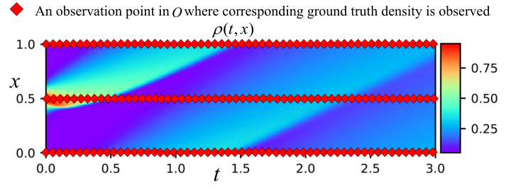
Fig. 7 shows the deployment of observation points for three loop detectors, where the detectors locate evenly on the road at , and . The traffic density records of those locations over time constitute the target values .
Using the same training process in Section IV-B, we conduct PIDL-based TSE experiments with different numbers of loop detectors. For each number of loop detectors, we make 100 trails with hyperparamters randomly selected between and . The minimal-achievable estimation errors of PIDL over the numbers of loop detectors are presented in Fig. 8, which are compared with the pure NN that is not regularized by the physics. The estimation errors of both methods decrease as more loop detectors are installed to collect data, and the PIDL outperforms the NN especially when the loop numbers are small. The results demonstrate that the PIDL-based approach is data efficient as it can handle the TSE task with fewer loop detectors for the traffic dynamics governed by the Greenshields-based LWR.
IV-D TSE and Parameter Discovery using Loop Detectors
This subsection justifies the ability of the PIDL architecture in Fig. 4 for dealing with both TSE and model parameter discovery. In this experiment, three model parameters , and are encoded as learning variables in PINN. We denote in this experiment. The residual and loss become
| (14) |
and
| (15) |
respectively. We use auxiliary points and other experimental configurations remain unchanged. We conduct PIDL-based TSE experiments using different numbers of loop detectors to solve . In addition to the traffic density estimation errors of , we evaluate the estimated model parameters using the relative error and present them in percentage. The results are shown in Table I, where the errors below the dashed line are acceptable.
| (%) | (%) | (%) | ||
|---|---|---|---|---|
| 2 | 6.007 | 982.22 | 362.50 | 1000 |
| 3 | 4.878 | 0.53 | 0.05 | 1.00 |
| 4 | 3.951 | 0.95 | 0.54 | 4.37 |
| 5 | 3.881 | 0.16 | 0.14 | 4.98 |
| 6 | 2.724 | 0.07 | 0.18 | 1.38 |
| 8 | 3.441 | 0.25 | 0.47 | 1.40 |
- •
stands for the number of loop detectors. are estimated parameters, compared to the true parameters .
From the table, we can see that the traffic density estimation errors improve as the number of loop detectors increases. When more than two loop detectors are used, the learning model parameters are able to converge to the true parameters . Specifically, for three loop detectors, in addition to a good traffic density estimation error of 4.878, the model parameters converge to , and , which are very close to the true ones. The results demonstrate that PIDL method can handle both TSE and model parameter discovery with three loop detectors for the traffic dynamics from the Greenshields-based LWR.
V PIDL for Three-Parameter-Based LWR
This example aims to show the ability of our method to handle the traffic dynamics governed by the three-parameter-based LWR.
The traffic flow model considered in this example is the same as Eqs. (10) except for a different flux function : three-parameter flux function [23, 64]. This flux function is triangle-shaped, which is a differentiable version of the piecewise linear Daganzo-Newell flux function [65, 66]. This function is defined as:
| (16) |
where , and are the three free parameters as the function is named. The parameters and control the maximum flow rate and critical density (where the flow is maximized), respectively. controls the roundness level of . In addition to the above-mentioned three parameters, and diffusion coefficient are also part of the model parameters.
Using the same domain and grid points setting in Section IV and initializing the dynamics with the bell-shaped density in Fig. 2, the numerical solution of three-parameter-based LWR is presented in Fig. 9. The parameters are given as , , , and . We treat the numerical solution as the ground truth and conduct our TSE experiments.

V-A PIDL Architecture Design
Using the definition of the residual value in Eq. (11), the corresponding PIDL architecture that encodes three-parameter-based LWR is shown in Fig. 10. Different from Fig. 4 where model parameters can be easily encoded as connecting weights, there are too many intermediate values involving the same model parameter, and thus, we cannot simply encode the model parameters as connecting weights. Instead, we use variable nodes (see the blue rectangular nodes in the graph) for holding model parameters, such that we can link the model parameter nodes to neurons that are directly related.
For the training loss, Eq. (12) is used, which includes the regularization of minimizing the residual and the difference between the density values at the two boundaries.
V-B TSE using Initial Observation
We justify the ability of the PIDL architecture in Fig. 10 for estimation of the traffic density field in Fig. 9 using the observation of the initial traffic density of the entire road at . The training data selection is the same as Section IV-B, except for that auxiliary points are used, because this is a relatively more complicated model.

The training process finds the optimal for PUNN, that minimizes the loss in Eq. (12). The results of applying the -parameterized PUNN to the three-parameter-based LWR dynamics estimation are presented in Fig. 11. The performance of the trained PUNN is satisfactory as the estimation achieves an relative error of , which is much smaller than the distinguishable error .
V-C TSE using Observation from Loop Detectors
We conduct PIDL-based TSE experiments with different numbers of loop detectors and compare the results with NN. Fig. 12 shows the PIDL approach achieves better errors than the pure NN, justifying the benefits of PIDL. A logarithmic error-axis is used for better visualizing the difference in estimation errors.
From the figure, we observe that the estimation errors decrease as more loop detectors are installed to collect data. A significant improvement in estimation quality is achieved when three loop detectors are installed, obtaining an error of compared to for two loop detectors. The NN needs more detectors to achieve these low errors.
V-D TSE and Parameter Discovery using Loop Detectors
This experiment focuses on using PIDL to address both TSE and model parameter discovery. Five learning variables need to be determined. The residual becomes:
| (17) |
and the in Eq. (15) is used in the training process. All experimental configurations and training process remain the same as Section V-C. We solve , and the results of traffic density estimation and model parameter discovery are presented in Table II. The errors below the dashed line are acceptable.
| (%) | (%) | (%) | (%) | (%) | ||
| 2 | 1.2040 | 58.19 | 153.72 | 1000 | 1000 | 99.98 |
| 3 | 7.550 | 54.15 | 124.52 | 1000 | 1000 | 99.95 |
| 4 | 1.004 | 59.07 | 72.63 | 381.31 | 14.60 | 6.72 |
| 5 | 3.186 | 2.75 | 4.03 | 6.97 | 0.29 | 3.00 |
| 6 | 1.125 | 0.69 | 2.49 | 2.26 | 0.49 | 7.56 |
| 8 | 7.619 | 1.03 | 2.43 | 3.60 | 0.30 | 7.85 |
| 12 | 5.975 | 1.83 | 1.65 | 1.24 | 0.82 | 5.70 |
- •
stands for the number of loop detectors. are estimated parameters, compared to the true parameters .
From the table, we observe that the PIDL architecture in Fig. 10 with five loop detectors can achieve a satisfactory performance on both traffic density estimation and model parameter discovery. In general, more loop detectors can help our model improve the TSE accuracy, as well as the convergence to the true model parameters. Specifically, for five loop detectors, an estimation error of is obtained, and the model parameters converge to , , , and , which are decently close to the ground truth. The results demonstrate that PIDL can handle both TSE and model parameter discovery with five loop detectors for the traffic dynamics governed by the three-parameter-based LWR.
VI PIDL-Based TSE on NGSIM Data
This section evaluates the PIDL-based TSE method using real traffic data, the Next Generation SIMulation (NGSIM) dataset22 2 www.fhwa.dot.gov/publications/research/operations/07030/index.cfm, and compares its performance to baselines.
VI-A NGSIM Dataset
NGSIM dataset provides detailed information about vehicle trajectories on several road scenarios. We focus on a segment of the US Highway 101 (US 101), monitored by a camera mounted on top of a high building on June 15, 2005. The locations and actions of each vehicle in the monitored region for a total of around 680 meters and 2,770 seconds were converted from camera videos. This dataset has gained a great attention in many traffic flow studies [67, 68, 69, 64].
We select the data from all the mainline lanes of the US 101 highway segment to calculate the average traffic density for approximately every 30 meters over a 30 seconds period. After preprocessing to remove the time when there are non-monitored vehicles running on the road (at the beginning and end of the video), there are 21 and 89 valid cells on the spatial and temporal dimensions, respectively. We treat the center of each cell as a grid point. Fig. 13 shows the spatio-temporal field of traffic density in the dataset. From the figure, we can observe that shockwaves backpropagate along the highway.

For TSE experiments in this section, loop detectors are used to provide observed data with a recording frequency of 30 seconds. By default, they are evenly installed on the highway segment. Since no ground-truth model parameters are available for NGSIM, we skip the parameter discovery experiments.
VI-B TSE Methods for Real Data
We first introduce the PIDL-based method for the real world TSE problem, and then, describe the baseline TSE methods.
VI-B1 PIDL-based Method
This method is based on a three-parameter-based LWR model introduced by [64], which is shown to be more accurate in describing the NGSIM data than the Greenshields-based LWR. To be specific, their model sets the diffusion coefficient to , and the traffic flow becomes , with the three-parameter flux defined in Eq. (16). The PIDL architecture is Fig. 10 is used. Because this is not a ring road, no boundary conditions are involved.
The three-parameter flux is calibrated using the data from loop detectors, which measure the traffic density (veh/km) and flow rate (veh/h) over time. Specifically, as shown in Fig. 14, we use fundamental diagram (FD) data (i.e., flow-density data points) to fit the three-parameter flux function (an FD curve). Least-squares fitting [64] is used to determine model parameters , , , and . The calibrated model is then encoded into PIDL.

We select auxiliary points from the grid (80%). The loss in Eq. (3) (with boundary terms removed) is used for training the PUNN using the observed data from loop detectors (i.e., both observation points and corresponding target density values ). After hyperparamter tuning, we present the minimal-achievable estimation errors. The same for other baselines by default.
VI-B2 Neural Netowrk (NN) Method
VI-B3 Long Short Term Memory (LSTM) based Method
This baseline method employs the LSTM architecture, which is customized from the LSTM-based TSE proposed by [38]. This model can be applied to our problem by leveraging the spatial dependency, i.e., to use the information of previous cells to estimate the traffic density of the next cell along the spatial dimension. We use the loss in Eq. (3) to train the LSTM-based model for TSE.
VI-B4 Extended Kalman Filter (EKF) Method
This method applies the extended Kalman filter (EKF), which is a nonlinear version of the Kalman filter that linearizes the models about the current estimation [70]. We use EKF to (1) estimate the whole spatio-temporal domain based on calibrated three-parameter-based LWR and (2) update its estimation based on the observed data from loop detectors.
To show the advantages of the proposed PIDL-based method, we limit our prior knowledge about the traffic flow to LWR and investigate that on top of this physical model, how well PIDL can take advantage of it. Under this setting, the TSE baselines we designed are either model-free (e.g., NN, LSTM) or LWR-based (e.g., EKF). TSE methods related to other traffic flow models, such as PW, ARZ and METANET will be left for future research.
VI-C Results and Discussion
We apply PIDL-based and baseline methods to TSE on the NGSIM dataset with different numbers of loop detectors. The results are presented in Fig. 15.
From Fig. 15, we can observe that the PIDL-based method can achieve satisfactory estimation (with an error below ) using eight loop detectors. In contrast, other baselines need twelve or more to reach acceptable errors. The EKF method performs better than the NN/LSTM-based methods when the number of loop detectors is , and NN/LSTM-based methods outperform EKF when sufficient data are available from more loop detectors.
The results are reasonable as EKF is a model-driven approach, making sufficient use of the traffic flow model to appropriately estimate unobserved values when limited data are available. However, the model cannot fully capture the complicated traffic dynamics in the real world, and as a result, the EKF’s performance flattens out. NN/LSTM-based methods are data-driven approaches which can make ample use of data to capture the dynamics. However, their data efficiency is low and large amounts of data are needed for accurate TSE. The PIDL-based method’s errors are generally below the baselines, because it can make efficient use of both the traffic flow model and observed data.
In addition to data efficiency, PIDL has the advantage to flexibly adjust the extent to which each of the data-driven and model-driven components will affect the training process. This flexibility is made possible by the hyperparamters and in the loss Eq. (3). Fig. 16 shows the ratios corresponding to the minimal-achievable estimation errors of the PIDL method presented in Fig. 15. When the number of loop detectors is small, more priorities should be given to the model-driven component (i.e., larger ratio) as the model is the only knowledge for making the estimation generalizable to the unobserved domain. When sufficient data are made available by a large number of loop detectors, more priorities should be given to the data-driven component (i.e., smaller ratio) as the traffic flow model model could be imperfect and can make counter effect to the estimation.
Computation time for training and estimation is another topic that TSE practitioners may concern. The results of computation time corresponding to Fig. 15 are presented in Fig. 17. Note that the training time and estimation time of EKF are the same because it conducts training and estimation simultaneously. For training, ML methods (NN and LSTM) consume more time than EKF because it takes thousands of iterations for ML methods to learn and converge, while EKF makes the estimation of the whole space per time step forward, which involves no iterative learning. PIDL takes the most time for training because it has to additionally backpropagete through the operations in PINN for computing the residual loss. For estimation, both PIDL and NN map the inputs directly to the traffic states and take the least computation time. LSTM operates in a recurrent way which takes more time to estimate. EKF needs to update the state transition and observation matrices for estimation at each time step, and thus, consumes the most time to finish the estimation.
VII Conclusion
In this paper, we introduced the PIDL framework to the TSE problem on highways using loop detector data and demonstrate the significant benefit of using LWR-based physics to inform the deep learning. This framework can be used to handle both traffic state estimation and model parameter discovery. The experiments on real highway traffic data show that PIDL-based approaches can outperform baseline methods in terms of estimation accuracy and data efficiency. Our work may inspire extended research on using sophisticated traffic models for more complicated traffic scenarios in the future.
Future work is threefold: First, we will consider to integrate more sophisticated traffic models, such as the PW, METANET and ARZ models, to PIDL for further improving TSE and model parameter discovery. Second, we will explore another type of observed data collected by probe vehicles, and study whether PIDL can conduct a satisfactory TSE task using these mobile data. Third, in practice, it is important to determine the optimal hyperparameters of the loss given the observed data. We will explore hyperparameters finding strategies, such as cross validations, to mitigate this issue.
Acknowledgment
The authors would like to thank Data Science Institute at Columbia University for providing a seed grant for this research.
References
- [1] T. Seo, A. M. Bayen, T. Kusakabe, and Y. Asakura, “Traffic state estimation on highway: A comprehensive survey,” Annual Reviews in Control, vol. 43, pp. 128–151, 2017.
- [2] D. S. Berry and F. H. Green, “Techniques for measuring over-all speeds in urban areas,” Highway Research Board Proceedings, vol. 29, pp. 311–318, 1949.
- [3] M. J. Lighthill and G. B. Whitham, “On kinematic waves II. A theory of traffic flow on long crowded roads,” Proceedings of the Royal Society of London. Series A. Mathematical and Physical Sciences, vol. 229, no. 1178, pp. 317–345, 1955.
- [4] P. I. Richards, “Shock waves on the highway,” Operations Research, vol. 4, no. 1, pp. 42–51, 1956.
- [5] M. Raissi, “Deep hidden physics models: Deep learning of nonlinear partial differential equations,” Journal of Machine Learning Research, vol. 19, no. 1, pp. 932–955, Jan. 2018.
- [6] M. Raissi and G. E. Karniadakis, “Hidden physics models: Machine learning of nonlinear partial differential equations,” Journal of Computational Physics, vol. 357, pp. 125–141, Mar. 2018.
- [7] H. J. Payne, “Model of freeway traffic and control,” Mathematical Model of Public System, pp. 51–61, 1971.
- [8] G. B. Whitham, “Linear and nonlinear waves,” John Wiley & Sons, vol. 42, 1974.
- [9] A. Aw, A. Klar, M. Rascle, and T. Materne, “Derivation of continuum traffic flow models from microscopic follow-the-leader models,” SIAM Journal on Applied Mathematics, vol. 63, no. 1, pp. 259–278, 2002.
- [10] H. M. Zhang, “A non-equilibrium traffic model devoid of gas-like behavior,” Transportation Research Part B: Methodological, vol. 36, no. 3, pp. 275–290, 2002.
- [11] M. Garavello, K. Han, and B. Piccoli, Models for vehicular traffic on networks. Springfield, MO: American Institute of Mathematical Sciences (AIMS), 2016, vol. 9.
- [12] Y. Wang, M. Papageorgiou, and A. Messmer, “Real-time freeway traffic state estimation based on extended Kalman filter: Adaptive capabilities and real data testing,” Transportation Research Part A: Policy and Practice, vol. 42, no. 10, pp. 1340–1358, 2008.
- [13] Y. Wang, M. Papageorgiou, A. Messmer, P. Coppola, A. Tzimitsi, and A. Nuzzolo, “An adaptive freeway traffic state estimator,” Automatica, vol. 45, no. 1, pp. 10–24, 2009.
- [14] X. Di, H. X. Liu, and G. A. Davis, “Hybrid extended Kalman filtering approach for traffic density estimation along signalized arterials: Use of global positioning system data,” Transportation Research Record, vol. 2188, no. 1, pp. 165–173, 2010.
- [15] L. Mihaylova, R. Boel, and A. Hegiy, “An unscented Kalman filter for freeway traffic estimation,” in Proceedings of the 11th IFAC Symposium on Control in Transportation Systems, Delft, Netherlands, 2006.
- [16] S. Blandin, A. Couque, A. Bayen, and D. Work, “On sequential data assimilation for scalar macroscopic traffic flow models,” Physica D: Nonlinear Phenomena, vol. 241, no. 17, pp. 1421–1440, 2012.
- [17] L. Mihaylova and R. Boel, “A particle filter for freeway traffic estimation,” in 43rd IEEE Conference on Decision and Control (CDC), Nassau, Bahamas, 2004, pp. 2106–2111.
- [18] M. Treiber and D. Helbing, “Reconstructing the spatio-temporal traffic dynamics from stationary detector data,” Cooperative Transportation Dynamics, vol. 1, no. 3, pp. 3.1–3.24, 2002.
- [19] B. Coifman, “Estimating travel times and vehicle trajectories on freeways using dual loop detectors,” Transportation Research Part A: Policy and Practice, vol. 36, no. 4, pp. 351–364, 2002.
- [20] J. A. Laval, Z. He, and F. Castrillon, “Stochastic extension of Newell’s three-detector method,” Transportation Research Record, vol. 2315, no. 1, pp. 73–80, 2012.
- [21] M. Kuwahara and et al, “Estimating vehicle trajectories on a motorway by data fusion of probe and detector data,” in 20th ITS World Congress, Tokyo 2013. Proceedings, Tokyo, Japan, 2013.
- [22] S. Blandin, J. Argote, A. M. Bayen, and D. B. Work, “Phase transition model of non-stationary traffic flow: Definition, properties and solution method,” Transportation Research Part B: Methodological, vol. 52, pp. 31–55, 2013.
- [23] S. Fan, M. Herty, and B. Seibold, “Comparative model accuracy of a data-fitted generalized Aw-Rascle-Zhang model,” Networks and Heterogeneous Media, vol. 9, no. 2, pp. 239–268, 2014.
- [24] K. Kawai, A. Takenouchi, M. Ikawa, and M. Kuwahara, “Traffic state estimation using traffic measurement from the opposing lane-error analysis based on fluctuation of input data,” Intelligent Transport Systems for Everyone’s Mobility, pp. 247–263, 2019.
- [25] S. E. G. Jabari, D. M. Dilip, D. Lin, and B. T. Thodi, “Learning traffic flow dynamics using random fields,” IEEE Access, vol. 7, pp. 130 566–130 577, 2019.
- [26] S. Paveri-Fontana, “On boltzmann-like treatments for traffic flow: a critical review of the basic model and an alternative proposal for dilute traffic analysis,” Transportation research, vol. 9, no. 4, pp. 225–235, 1975.
- [27] G. A. Davis and J. G. Kang, “Estimating destination-specific traffic densities on urban freeways for advanced traffic management,” Transportation Research Record, no. 1457, pp. 143–148, 1994.
- [28] J.-G. Kang, Estimation of destination-specific traffic densities and identification of parameters on urban freeways using Markov models of traffic flow. University of Minnesota, 1995.
- [29] S. E. Jabari and H. X. Liu, “A stochastic model of traffic flow: Theoretical foundations,” Transportation Research Part B: Methodological, vol. 46, no. 1, pp. 156–174, 2012.
- [30] B. L. Smith, W. T. Scherer, and J. H. Conklin, “Exploring imputation techniques for missing data in transportation management systems,” Transportation Research Record, vol. 1836, no. 1, pp. 132–142, 2003.
- [31] C. Chen, J. Kwon, J. Rice, A. Skabardonis, and P. Varaiya, “Detecting errors and imputing missing data for single-loop surveillance systems,” Transportation Research Record, vol. 1855, no. 1, pp. 160–167, 2003.
- [32] M. Zhong, P. Lingras, and S. Sharma, “Estimation of missing traffic counts using factor, genetic, neural, and regression techniques,” Transportation Research Part C: Emerging Technologies, vol. 12, no. 2, pp. 139–166, 2004.
- [33] L. Li, Y. Li, and Z. Li, “Efficient missing data imputing for traffic flow by considering temporal and spatial dependence,” Transportation Research Part C: Emerging Technologies, vol. 34, pp. 108–120, 2013.
- [34] H. Tan, Y. Wu, B. Cheng, W. Wang, and B. Ran, “Robust missing traffic flow imputation considering nonnegativity and road capacity,” Mathematical Problems in Engineering, 2014.
- [35] S. Tak, S. Woo, and H. Yeo, “Data-driven imputation method for traffic data in sectional units of road links,” IEEE Transactions on Intelligent Transportation Systems, vol. 17, no. 6, pp. 1762–1771, 2016.
- [36] D. Ni and J. D. Leonard, “Markov chain Monte Carlo multiple imputation using Bayesian networks for incomplete intelligent transportation systems data,” Transportation Research Record, vol. 1935, no. 1, pp. 57–67, 2005.
- [37] N. G. Polson and V. O. Sokolov, “Deep learning for short-term traffic flow prediction,” Transportation Research Part C: Emerging Technologies, vol. 79, pp. 1–17, 2017.
- [38] W. Li, J. Hu, Z. Zhang, and Y. Zhang, “A novel traffic flow data imputation method for traffic state identification and prediction based on spatio-temporal transportation big data,” in Proceedings of International Conference of Transportation Professionals (CICTP), Shanghai, China, 2017, pp. 79–88.
- [39] Z. Zheng, Y. Yang, J. Liu, H.-N. Dai, and Y. Zhang, “Deep and embedded learning approach for traffic flow prediction in urban informatics,” IEEE Transactions on Intelligent Transportation Systems, vol. 20, no. 10, pp. 3927–3939, 2019.
- [40] J. Tang, X. Zhang, W. Yin, Y. Zou, and Y. Wang, “Missing data imputation for traffic flow based on combination of fuzzy neural network and rough set theory,” Journal of Intelligent Transportation Systems, pp. 1–16, 2020.
- [41] A. Hofleitner, R. Herring, and A. Bayen, “Arterial travel time forecast with streaming data: A hybrid approach of flow modeling and machine learning,” Transportation Research Part B: Methodological, vol. 46, no. 9, pp. 1097–1122, 2012.
- [42] S. Wang, W. Huang, and H. K. Lo, “Traffic parameters estimation for signalized intersections based on combined shockwave analysis and Bayesian network,” Transportation Research Part C: Emerging Technologies, vol. 104, pp. 22–37, 2019.
- [43] X. Jia, A. Karpatne, J. Willard, M. Steinbach, J. Read, P. C. Hanson, H. A. Dugan, and V. Kumar, “Physics guided recurrent neural networks for modeling dynamical systems: Application to monitoring water temperature and quality in lakes,” arXiv preprint arXiv:1810.02880, 2018.
- [44] Y. Yuan, X. T. Yang, Z. Zhang, and S. Zhe, “Macroscopic traffic flow modeling with physics regularized gaussian process: A new insight into machine learning applications,” arXiv preprint arXiv:2002.02374, 2020.
- [45] Z. Wang, W. Xing, R. Kirby, and S. Zhe, “Physics regularized gaussian processes,” arXiv preprint arXiv:2006.04976, 2020.
- [46] Y. Yang and P. Perdikaris, “Adversarial uncertainty quantification in physics-informed neural networks,” Journal of Computational Physics, vol. 394, pp. 136–152, 2019.
- [47] M. Raissi, Z. Wang, M. S. Triantafyllou, and G. E. Karniadakis, “Deep learning of vortex-induced vibrations,” Journal of Fluid Mechanics, vol. 861, pp. 119–137, 2019.
- [48] Z. Fang and J. Zhan, “Physics-informed neural network framework for partial differential equations on 3D surfaces: Time independent problems,” IEEE Access, 2020.
- [49] M. Raissi, A. Yazdani, and G. E. Karniadakis, “Hidden fluid mechanics: Learning velocity and pressure fields from flow visualizations,” Science, vol. 367, no. 6481, pp. 1026–1030, 2020.
- [50] M. Gulian, M. Raissi, P. Perdikaris, and G. Karniadakis, “Machine learning of space-fractional differential equations,” SIAM Journal on Scientific Computing, vol. 41, no. 4, pp. A2485–A2509, 2019.
- [51] G. Pang, L. Lu, and G. E. Karniadakis, “fPINNs: Fractional physics-informed neural networks,” SIAM Journal on Scientific Computing, vol. 41, no. 4, pp. A2603–A2626, 2019.
- [52] A. Karpatne, G. Atluri, and et al, “Theory-guided data science: A new paradigm for scientific discovery from data,” IEEE Transactions on Knowledge and Data Engineering, vol. 29, no. 10, pp. 2318–2331, 2017.
- [53] A. G. Baydin, B. A. Pearlmutter, A. A. Radul, and J. M. Siskind, “Automatic differentiation in machine learning: A survey,” Journal of Machine Learning Research, vol. 18, no. 1, pp. 5595–5637, 2017.
- [54] B. Greenshields, W. Channing, and H. Miller, “A study of traffic capacity,” Highway Research Board Proceedings, vol. 14, pp. 448–477, 1935.
- [55] P. Nelson, “Traveling-wave solutions of the diffusively corrected kinematic-wave model,” Mathematical and Computer Modelling, vol. 35, pp. 561–579, 2002.
- [56] J. Li, H. Wang, Q.-Y. Chen, and D. Ni, “Traffic viscosity due to speed variation: Modeling and implications,” Mathematical and Computer Modelling, vol. 52, pp. 1626–1633, 2010.
- [57] R. Burger, P. Mulet, and L. M. Villada, “Regularized nonlinear solvers for IMEX methods applied to diffusively corrected multispecies kinematic flow models,” SIAM Journal on Scientific Computing, vol. 35, no. 3, pp. B751–B777, 2013.
- [58] C. D. Acosta, R. Burger, and C. E. Mejia, “Efficient parameter estimation in a macroscopic traffic flow model by discrete mollification,” Transportmetrica A: Transport Science, vol. 11, no. 8, pp. 702–715, 2015.
- [59] R. Burger and I. Kroker, “Hybrid stochastic Galerkin finite volumes for the diffusively corrected Lighthill-Whitham-Richards traffic model,” in Finite Volumes for Complex Applications VIII - Hyperbolic, Elliptic and Parabolic Problems. Cham: Springer International Publishing, 2017, pp. 189–197.
- [60] S. K. Godunov, “A difference method for numerical calculation of discontinuous solutions of the equations of hydrodynamics,” Matematicheskii Sbornik, vol. 89, no. 3, pp. 271–306, 1959.
- [61] X. Glorot and Y. Bengio, “Understanding the difficulty of training deep feedforward neural networks,” in Proceedings of the 30th International Conference on Artificial Intelligence and Statistics (AISTATS), Chia Laguna, Sardinia, Italy, 2010, pp. 249–256.
- [62] O. Konur, D. P. Kingma, and J. Ba, “Adam: A method for stochastic optimization,” in Proceedings of the International Conference on Learning Representations (ICLR), San Diego, CA, USA, 2015.
- [63] R. H. Byrd, P. Lu, J. Nocedal, and C. Zhu, “A limited memory algorithm for bound constrained optimization,” SIAM Journal on Scientific Computing, vol. 16, no. 5, pp. 1190–1208, 1995.
- [64] S. Fan and B. Seibold, “Data-fitted first-order traffic models and their second-order generalizations: Comparison by trajectory and sensor data,” Transportation Research Record, vol. 2391, no. 1, pp. 32–43, 2013.
- [65] C. Daganzo, “The cell transmission model: A dynamic representation of highway traffic consistent with the hydrodynamic theory,” Transportation Research Part B: Methodological, vol. 28, no. 4, pp. 269–287, 1994.
- [66] G. F. Newell, “A simplified theory of kinematic waves in highway traffic, part II: Queueing at freeway bottlenecks,” Transportation Research Part B: Methodological, vol. 27, no. 4, pp. 289–303, 1993.
- [67] N. Chiabaut, L. Leclercq, and C. Buisson, “From heterogeneous drivers to macroscopic patterns in congestion,” Transportation Research Part B: Methodological, vol. 44, no. 2, pp. 299–308, 2010.
- [68] J. A. Laval and L. Leclercq, “A mechanism to describe the formation and propagation of stop-and-go waves in congested freeway traffic,” Philosophical Transactions of the Royal Society A: Mathematical, Physical and Engineering Sciences, vol. 368, no. 1928, pp. 4519–4541, 2010.
- [69] M. Montanino and V. Punzo, “Making NGSIM data usable for studies on traffic flow theory: Multistep method for vehicle trajectory reconstruction,” Transportation Research Record, vol. 2390, no. 1, pp. 99–111, 2013.
- [70] Y. Kim and H. Bang, “Introduction to Kalman filter and its applications,” in Kalman Filter. London, UK: IntechOpen, 2018, pp. 1–9.