Scale factor point spread function matching: beyond aliasing in image resampling

Observed samples (pixels/voxels) in medical images are not direct Dirac impulse measurements of a biological scene, but are typically samples from the convolution of the unobservable biological scene with an observation kernel, i.e. they have an associated point spread function (PSF). This PSF is commonly a property of the acquisition or reconstruction system. For example, 3D MRI images have approximately Gaussian PSFs due to several factors, including the low-pass filters in the receiver coils, while CT and PET images have spatially variant PSFs dependent on many parameters including the image reconstruction algorithm.

In this work, we propose to associate a PSF to each image, whether it directly arises from an imaging device or is the result of further transformation or processing, and refer to this as the scale factor PSF (sfPSF) by analogy with the scale factor used in scale space theory [4]. In the case where the image directly arises from an imaging device with known PSF, the sfPSF is simply taken as the closest Gaussian approximation. When the actual PSF associated with a given image is unkown, without loss of generality the nominal sfPSF is assumed to be a Gaussian $\mathcal{G}_{\Sigma}$, where the covariance matrix $\Sigma$ is diagonal and the full-width-half-maximum (FWHM) of the Gaussian PSF is matched to the voxel size $D=\{D_{x},D_{y},D_{z}\}$: $\Sigma=(2\sqrt{2\log 2})^{-2}\diag(D_{x}^{2},D_{y}^{2},D_{z}^{2})$. The relevance of the sfPSF will become clear in the following section. Intuitively, when an image with an associated sfPSF is smoothed, the resulting smoothed image will have larger sfPSF. Conversely, when an image is upsampled, the resulting image will be associated with the same sfPSF as the source image (in world coordinates).

In medical images, frequencies commonly approach the Nyquist limit of their representation (e.g. full k-space sampling in MRI). If one affinely transforms an image onto its own grid with an affine transformation which has a determinant greater than 1, i.e. spatially compressing the samples, or transforms an image into a lower resolution grid, then the Nyquist criterion is not satisfied with typical interpolation. This sub-Nyquist sampling introduces frequency aliasing and loss of information.

In scale-space and pyramidal approaches, when downsampling an image by a factor of $k=2$, the original image is typically pre-convolved with a Gaussian filter with variance $\sigma_{P}=0.7355$. Applying the notion of sfPSF and the notations introduced above, we specify $\mathcal{G}_{{\Sigma}_{S}}$ and $\mathcal{G}_{{\Sigma}_{T}}$ as the source image and target grid nominal sfPSFs respectively. Following the scale space methodology [4], sfPSF matching consists of finding the best scale-matching PSF $\mathcal{G}_{{\Sigma}_{P}}$ that, when combined with the source sfPSF, provides the best approximation of the target sfPSF. If the sfPSFs are Gaussian, then the covariance of $\mathcal{G}_{{\Sigma}_{P}}$ can be obtained through simple covariance addition ${{{\Sigma}_{T}}={{\Sigma}_{S}}}+{{\Sigma}_{P}}$. In the downsampling example above, without additional knowledge, we have $\FWHM_{T}=k=2$ and $\FWHM_{S}=1$. We therefore get $\Sigma_{P}=\Sigma_{T}-\Sigma_{S}=(k^{2}-1^{2})(2\sqrt{2\log{2}})^{-2}\Id$ or, in this case, $\sigma_{P}=0.7355$. This is equivalent to finding the best Fourier domain filter that limits the bandwidth of the source image frequencies to the representable Nyquist frequencies on the target grid. Similar filtering would be necessary to avoid aliasing when rigidly resampling high resolution images to a lower resolution, e.g. high resolution anatomical MRI and CT images or binary segmentations are transformed to lower resolution MRI (2D FLAIR), metabolic (PET), microstructural (DWI) and functional (fMRI) images. In this work we propose to compensate for the differences in sfPSF when resampling to arbitrary grid sizes under global (affine) or local (non-linear) spatial transformations.

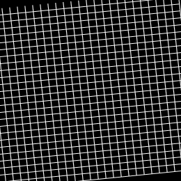
Before presenting our methodological contribution in detail, we illustrate the sfPSF performance in comparison with standard interpolation on a synthetic phantom (Fig. 1) with a low frequency object (square) overlaid on a high-frequency pattern (to highlight aliasing). This phantom is resampled to a grid with 3 times less resolution per axis. Note that the proposed sfPSF method appropriately integrates out high frequencies without introducing aliasing.

In the affine transformation $\mathcal{A}$ scenario from the space of $T$ to $S$, the source image can be pre-convolved with an anti-aliasing filter with covariance $\Sigma_{P}^{S}+\Sigma_{S}=\mathcal{A}\cdot\Sigma_{T}\cdot\mathcal{A}^{\intercal}$ and then resampled using classical interpolation. Note that $\Sigma_{P}^{S}$ is now defined in the space of $S$.

In the general non-linear spatial transformation case, a similar but spatially-variant pre-filtering procedure could be applied by relying on a local affine approximation of the spatial transformation, i.e. using the jacobian matrix. This solution might provide useful results but because the sfPSF matching, or smoothing, is performed before the spatial transformation, and the sfPSF potentially has a large spatial extent, it can be seen as disregarding the non-homogeneous distribution of the samples in target space $T$. Instead, we propose to model and perform the sfPSF matching in the space of $T$ and thus rely on $\Sigma_{P}^{T}$.

Let $\mathcal{F}_{S\leftarrow T}(\mathbf{v})$ be a spatial transformation mapping the location $\mathbf{v}=(v_{x},v_{y},v_{z})$ from the space of $T$ to that of $S$, given either an affine or non-linear transformation. Let $\mathcal{A}_{S\leftarrow T}(\mathbf{v})$ be the jacobian matrix of $\mathcal{F}$ at $\mathbf{v}$ which provides the best linear approximation of $\mathcal{F}$ at $\mathbf{v}$. Following our previous derivations we have $\Sigma_{P}^{S}(\mathbf{v})+\Sigma_{S}\approx\mathcal{A}_{S\leftarrow T}(\mathbf{v})\cdot\Sigma_{T}\cdot\mathcal{A}_{S\leftarrow T}^{\intercal}(\mathbf{v})$. Thus, given $\Sigma_{P}^{S}(\mathbf{v})=\mathcal{A}_{S\leftarrow T}(\mathbf{v})\cdot\Sigma_{P}^{T}(\mathbf{v})\cdot\mathcal{A}_{S\leftarrow T}^{\intercal}(\mathbf{v})$ we now want $\Sigma_{P}^{T}(\mathbf{v})+\mathcal{A}_{S\leftarrow T}^{-1}(\mathbf{v})\cdot\Sigma_{S}\cdot\mathcal{A}_{S\leftarrow T}^{-\intercal}(\mathbf{v})\approx\Sigma_{T}$. In other words, we want to find a symmetric positive semi-definite covariance $\Sigma_{P}^{T}(\mathbf{v})$ that, when combined with the affinely transformed covariance $\Sigma_{S}^{T}(\mathbf{v})=\mathcal{A}_{S\leftarrow T}^{-1}(\mathbf{v})\cdot\Sigma_{S}\cdot\mathcal{A}_{S\leftarrow T}^{-\intercal}(\mathbf{v})$, best approximates $\Sigma_{T}$. Under the typical assumption that the nominal sfPSF $\Sigma_{T}$ is diagonal, this approximation is given by $\tilde{\Sigma_{P}^{T}}(\mathbf{v})=\max(\Sigma_{T}-\lambda(\mathbf{v}),0)$ with $\lambda(\mathbf{v})$ being a diagonal scaling matrix containing the components of $\Sigma_{S}^{T}(\mathbf{v})$ obtained through polar decomposition and $max(\cdot,\cdot)$ is the element-wise maximum operator between two matrices. It is important to note that under regimes where the Nyquist limit is not violated, e.g. upsampling and rigid transformation between isotropic grids, the proposed method reverts to standard resampling as the sfPSF would become a Dirac.

Under the sampling theorem, replacing the Gaussian in Eq.1 with Sinc should produce the theoretically best alias-free results. Knowing that this work focuses on obtaining realistic PSF’s rather than the least aliased one, we note 3 problems with Sinc resampling that are addressed with the proposed method: First, Sinc is only optimal if the discretised sampling scheme of Eq.1 is replaced with an integral. Second, sincs are optimal from a bandlimit point of view, but are poor approximations of real PSFs, e.g. PET images have aproximate Gaussian PSF larger than the voxel size. Finally, sincs cannot be used for signal-limited images (probabilistic segmentations bounded from 0 to 1), as it would produce negative probabilities. Conversely, Gaussians do not have this problem.

30 healthy control subjects were obtained from the ADNI2 database. All subjects had an associated T1-weighted MRI image, acquired at 1.1$\times$1$\times$1$mm$ voxel size, and a ¹⁸F-FDG PET image, reconstructed at 3$\times$3$\times$3$mm$. For this selected subset of ADNI2, all data (MRI and PET) were acquired on the same scanner with the same scanning parameters, thus removing acquisition confounds. While the effective PSF of PET images can be between 3 and 6$mm$ FWHM, in these experiments we will assume a PSF with 3$mm$ FWHM.

Frequency domain analysis was used to assess whether resampling images under non-linear transformation respects the Nyquist limit and to test whether the proposed method can mitigate any error. The 30 T1 MRIs were zero padded by a factor of 2 in the frequency domain (0.55$\times$0.5$\times$0.5$mm$ voxel size), doubling the representable frequencies. Fig. 2 shows two upsampled images and their frequency magnitude. Note the empty power spectrum outside the Nyquist band (white box).

29 upsampled T1 images were affinely [7] and then non-rigidly [8] registered to the remaining image using standard algorithms. Each upsampled image was resampled to the space of the remaining image using both a three-lobed truncated sinc resampling, and the proposed Gaussian sfPSF method (see Fig. 2). The Gaussian sfPSF was set to 1.1$\times$1$\times$1$mm$ FWHM for both $\Sigma_{S}$ and $\Sigma_{T}$. Note that, as expected, supra-Nyquist frequencies are created when using sinc interpolation. These frequencies are greatly suppressed when using the proposed method. Analysis of the power spectra of the 29 resampled images showed an average power suppression of 94.4% for frequencies above the Nyquist band when using the Gaussian PSF instead of sinc interpolation. This power suppression results in an equivalent reduction of aliasing at the original resolution.

To demonstrate clinically relevant consequences of aliasing, we tested the effect of resampling within the context of segmentation propagation and partial volume estimation. Specifically, T1 images are segmented into 98 different regions using multi-atlas label propagation and fusion [9] based on the Neuromorphometrics, Inc. labels. The T1 images were then rigidly registered [7] to the PET data, and each one of the segmented regions was resampled to the PET data using both linear interpolation and the Gaussian sfPDF. Linear was chosen here due to the signal-limited $[0,1]$ nature of probabilities. Example results are shown in Fig. 3.

As all the segmentations are probabilistic, volume was estimated as the sum of all probabilities for all voxels $\mathbf{v}$ times the voxel size $\mathcal{V}$. The volume was estimated in the original T1 space ($V_{HR}$), and in the PET space after linear ($V_{TRI}$) and the Gaussian sfPSF ($V_{sfPSF}$) resampling. Similar volumes were obtained when the probabilistic segmentations were thresholded at 0.5. The relative volume difference RVD$=(V_{sfPSF}-V_{HR})/V_{HR}$ and its absolute value, ARVD $=|$RVD$|$, were estimated for each of the 30 subjects, 98 cortical regions and 2 resampling methods. The RVD and ARVD were averaged over all subjects for each region, resulting in 98 mean RVD and ARVD values per region, per method. These values are plotted in Fig. 4. A Parzen window mean and STD are also plotted in the same figure. Both resampling methods are unbiased according to the mean RVD. However, the Gaussian sfPSF method provides significantly lower ($p<10^{-4}$ - Wilcoxon signed-rank test) errors in terms of mean ARVD for all regions, especially in smaller regions where linear resampling can introduce up to 8% mean absolute volume difference. An 8% mean difference implies even larger local errors, resulting in detrimental effects in partial volume/ compartment modelling, and when estimating biomarkers that rely on structural segmentations.

This work was supported by the EPSRC (EP/H046410/1, EP/J020990/1, EP/K005278), the MRC (MR/J01107X/1), the EU-FP7 (FP7-ICT-2011-9-601055), the NIHR BRC UCLH/UCL HII (BW.mn.BRC10269), and the UCL Leonard Wolfson Experimental Neurology Centre (PR/ylr/18575).

References

- [1] Meijering, E.H.W., Niessen, W.J., Pluim, J.P.W., Viergever, M.A.: Quantitative comparison of sinc-approximating kernels for medical image interpolation. In: Proc. MICCAI’99. Springer Berlin Heidelberg (1999) 210–217
- [2] Pluim, J.P., Maintz, J.B.A., Viergever, M.A.: Mutual information matching and interpolation artifacts. In: SPIE Medical Imaging. Volume 3661., SPIE Press (May 1999) 56–65
- [3] Aganj, I., Yeo, B.T.T., Sabuncu, M.R., Fischl, B.: On removing interpolation and resampling artifacts in rigid image registration. IEEE Trans. Image Process. 22(2) (February 2013) 816–827
- [4] Lindeberg, T.: Scale-space for discrete signals. IEEE Trans. Pattern Anal. Mach. Intell. 12(3) (1990) 234–254
- [5] Unser, M., Neimark, M., Lee, C.: Affine transformations of images: a least squares formulation. In: Proc. ICIP’94. Volume 3. (1994) 558–561
- [6] Arigovindan, M., Sühling, M., Hunziker, P., Unser, M.: Variational image reconstruction from arbitrarily spaced samples: A fast multiresolution spline solution. IEEE Trans. Image Process. 14(4) (2005) 450–460
- [7] Modat, M., Cash, D.M., Daga, P., Winston, G.P., Duncan, J.S., Ourselin, S.: Global image registration using a symmetric block-matching approach. Journal of Medical Imaging 1(2) (July 2014) 024003–024003
- [8] Modat, M., Ridgway, G.R., Taylor, Z.A., Lehmann, M., Barnes, J., Hawkes, D.J., Fox, N.C., Ourselin, S.: Fast free-form deformation using graphics processing units. Computer Methods and Programs in Biomedicine 98(3) (June 2010) 278–284
- [9] Cardoso, M., Modat, M., Wolz, R., Melbourne, A., Cash, D., Rueckert, D., Ourselin, S.: Geodesic information flows: Spatially-variant graphs and their application to segmentation and fusion. IEEE TMI (in press) (2015)
- [10] Higham, N.J.: Computing a nearest symmetric positive semidefinite matrix. Linear Algebra Appl. 103 (1988) 103–118
- [11] Schröcker, H.P.: Uniqueness results for minimal enclosing ellipsoids. Comput. Aided Geom. Des. 25(9) (2008) 756–762
Draft Appendix
Let and be 2 symmetric positive definite (SPD) matrices representing covariance matrices. We are looking for the smallest symmetric positive semi-definite (SPSD) matrix such that is larger than .
Some useful tools and properties
A matrix is SPSD if