GEO: Enhancing Combinatorial Optimization with Classical and Quantum Generative Models
Abstract
We introduce a new framework that leverages machine learning models known as generative models to solve optimization problems. Our Generator-Enhanced Optimization (GEO) strategy is flexible to adopt any generative model, from quantum to quantum-inspired or classical, such as Generative Adversarial Networks, Variational Autoencoders, or Quantum Circuit Born Machines, to name a few. Here, we focus on a quantum-inspired version of GEO relying on tensor-network Born machines, and referred to hereafter as TN-GEO. We present two prominent strategies for using TN-GEO. The first uses data points previously evaluated by any quantum or classical optimizer, and we show how TN-GEO improves the performance of the classical solver as a standalone strategy in hard-to-solve instances. The second strategy uses TN-GEO as a standalone solver, i.e., when no previous observations are available. Here, we show its superior performance when the goal is to find the best minimum given a fixed budget for the number of function calls. This might be ideal in situations where the cost function evaluation can be very expensive. To illustrate our results, we run these benchmarks in the context of the portfolio optimization problem by constructing instances from the S&P 500 and several other financial stock indexes. We show that TN-GEO can propose unseen candidates with lower cost function values than the candidates seen by classical solvers. This is the first demonstration of the generalization capabilities of quantum-inspired generative models that provide real value in the context of an industrial application. We also comprehensively compare state-of-the-art algorithms in a generalized version of the portfolio optimization problem. The results show that TN-GEO is among the best compared to these state-of-the-art algorithms; a remarkable outcome given the solvers used in the comparison have been fine-tuned for decades in this real-world industrial application. We see this as an important step toward a practical advantage with quantum-inspired models and, subsequently, with quantum generative models.
I Introduction
Along with machine learning and the simulation of materials, combinatorial optimization is one of top candidates for practical quantum advantage. That is, the moment where a quantum-assisted algorithm outperforms the best classical algorithms in the context of a real-world application with a commercial or scientific value. There is an ongoing portfolio of techniques to tackle optimization problems with quantum subroutines, ranging from algorithms tailored for quantum annealers (e.g., Refs. Kadowaki and Nishimori 1998; Farhi et al. 2001), gate-based quantum computers (e.g., Refs. Edward Farhi 2014; Hadfield et al. 2019) and quantum-inspired (QI) models based on tensor networks (e.g., Ref. Mugel et al. 2020).
Regardless of the quantum optimization approach proposed to date, there is a need to translate the real-world problem into a polynomial unconstrained binary optimization (PUBO) expression – a task which is not necessarily straightforward and that usually results in an overhead in terms of the number of variables. Specific real-world use cases illustrating these PUBO mappings are depicted in Refs. Perdomo-Ortiz et al. 2012 and Perdomo-Ortiz et al. 2019. Therefore, to achieve practical quantum advantage in the near-term, it would be ideal to find a quantum optimization strategy that can work on arbitrary objective functions, bypassing the translation and overhead limitations raised here.
In our work, we offer a solution to these challenges by proposing a novel generator-enhanced optimization (GEO) framework which leverage the power of (quantum or classical) generative models. This family of solvers can scale to large problems where combinatorial problems become intractable in real-world settings. Since our optimization strategy does not rely on the details of the objective function to be minimized, it is categorized in the group of so-called black-box solvers. Another highlight of our approach is that it can utilize available observations obtained from attempts to solve the optimization problem. These initial evaluations can come from any source, from random search trials to tailored state-of-the-art (SOTA) classical or quantum optimizers for the specific problem at hand.
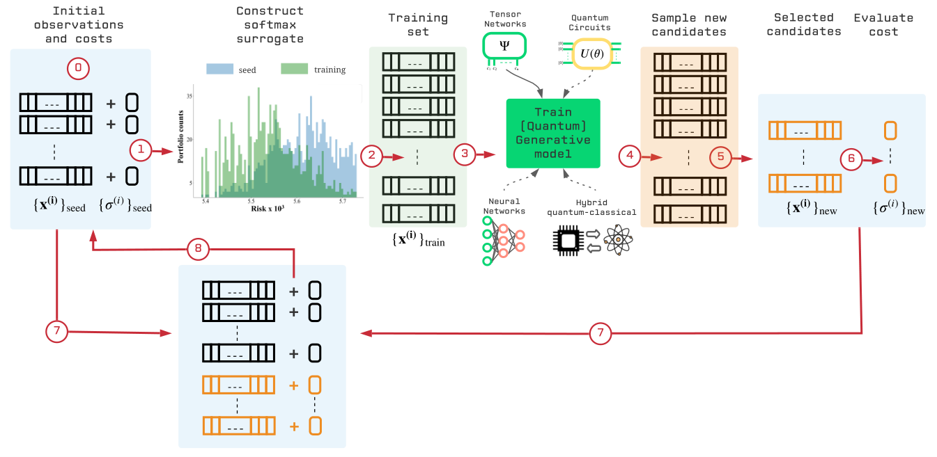
Our GEO strategy is based on two key ideas. First, the generative-modeling component aims to capture the correlations from the previously observed data (step 0-3 in Fig. 1). Second, since the focus here is on a minimization task, the (quantum) generative models need to be capable of generating new “unseen” solution candidates which have the potential to have a lower value for the objective function than those already “seen” and used as the training set (step 4-6 in Fig. 1). This exploration towards unseen and valuable samples is by definition the fundamental concept behind generalization: the most desirable and important feature of any practical ML model. We will elaborate next on each of these components and demonstrate these two properties in the context of the tensor-network-based generative models and its application to a non-deterministic polynomial-time hard (NP-hard) version of the portfolio optimization in finance.
To the best of our knowledge, this is the first optimization strategy proposed to do an efficient blackbox exploration of the objective-function landscape with the help of generative models. Although other proposal leveraging generative models as a subroutine within the optimizer have appeared recently since the publication of our manuscript (e.g., see GFlowNets Bengio et al. 2021 and the variational neural annealing Hibat-Allah et al. 2021 algorithms), our framework is the only capable of both, handling arbitrary cost functions and also with the possibility of swapping the generator for a quantum or quantum-inspired implementation. GEO also has the enhanced feature that the more data is available, the more information can be passed and used to train the (quantum) generator.
In this work, we highlight the different features of GEO by performing a comparison with alternative solvers, such as Bayesian optimizers and generic solvers like simulated annealing. In the case of the specific real-world large-scale application of portfolio optimization, we compare against the SOTA optimizers and show the competitiveness of our approach. These results are presented in Sec. III. Next, in Sec. II, we present the GEO approach and its range of applicability.
II Quantum-Enhanced Optimization with Generative Models
As shown in Fig. 1, depending on the GEO specifics we can construct an entire family of solvers whose generative modeling core range from classical, QI or quantum circuit (QC) enhanced, or hybrid quantum-classical model. These options can be realized by utilizing, for example, Boltzmann machines Cheng et al. 2018 or Generative Adversarial Networks (GAN) Goodfellow et al. 2014, Tensor-Network Born Machines (TNBM) Cheng et al. 2017, Quantum Circuit Born Machines (QCBM)Benedetti et al. 2018 or Quantum-Circuit Associative Adversarial Networks (QC-AAN)Rudolph et al. 2020 respectively, to name just a few of the many options for this probabilistic component.
QI algorithms come as an interesting alternative since these allow one to simulate larger scale quantum systems with the help of efficient tensor-network (TN) representations. Depending on the complexity of the TN used to build the quantum generative model, one can simulate from thousands of problem variables to a few tens, the latter being the limit of simulating an universal gate-based quantum computing model. This is, one can control the amount of quantum resources available in the quantum generative model by choosing the QI model.
Therefore, from all quantum generative model options, we chose to use a QI generative model based on TNs to test and scale our GEO strategy to instances with a number of variables commensurate with those found in industrial-scale scenarios. We refer to our solver hereafter as TN-GEO. For the training of our TN-GEO models we followed the work of Han et al. Han et al. 2018 where they proposed to use Matrix Product States (MPS) to build the unsupervised generative model. The latter extends the scope from early successes of quantum-inspired models in the context of supervised ML Stoudenmire and Schwab 2016; Efthymiou et al. 2019; Roberts et al. 2019; Fishman et al. 2020.
In this paper we will discuss two modes of operation for our family of quantum-enhanced solvers:
- •
In TN-GEO as a ”booster” we leverage past observations from classical (or quantum) solvers. To illustrate this mode we use observations from simulated annealing (SA) runs. Simulation details are provided in Appendix A.5.
- •
In TN-GEO as a stand-alone solver all initial cost function evaluations are decided entirely by the quantum-inspired generative model, and a random prior is constructed just to give support to the target probability distribution the MPS model is aiming to capture. Simulation details are provided in Appendix A.6.
III Results and Discussion
To illustrate the implementation for both of these settings we tested their performance on an NP-hard version of the portfolio optimization problem with cardinality constraints. The selection of optimal investment on a specific set of assets, or portfolios, is a problem of great interest in the area of quantitative finance. This problem is of practical importance for investors, whose objective is to allocate capital optimally among assets while respecting some investment restrictions. The goal of this optimization task, introduced by Markowitz Markowitz 1952, is to generate a set of portfolios that offers either the highest expected return (profit) for a defined level of risk or the lowest risk for a given level of expected return. In this work, we focus in two variants of this cardinality constrained optimization problem. The first scenario aims to choose portfolios which minimize the volatility or risk given a specific target return (more details are provided in Appendix A.1.) To compare with the reported results from the best performing SOTA algorithms, we ran TN-GEO in a second scenario where the goal is to choose the best portfolio given a fixed level of risk aversion. This is the most commonly used version of this optimization problem when it comes to comparison among SOTA solvers in the literature (more details are provided in Appendix A.2).
III.1 TN-GEO as a booster for any other combinatorial optimization solver
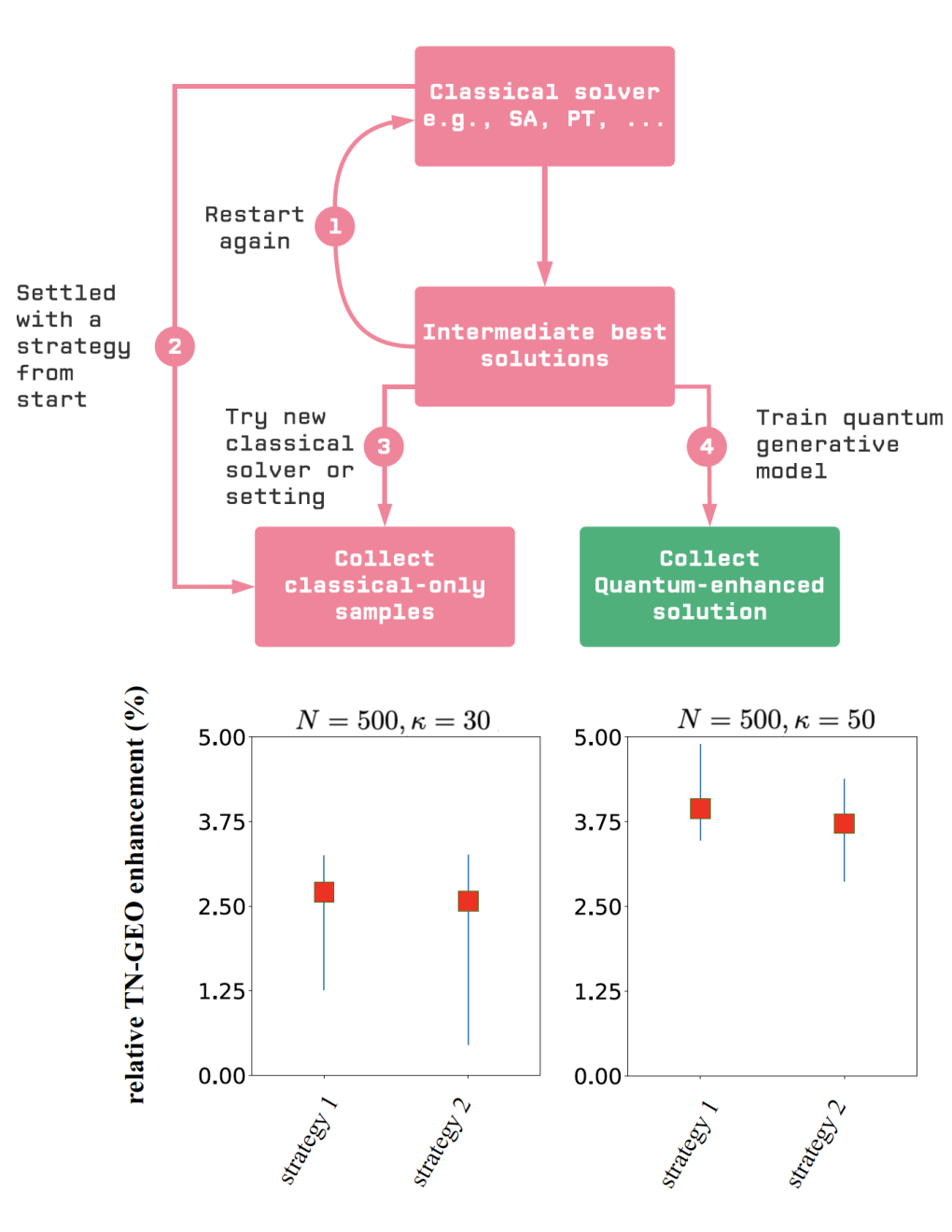
In Fig. 2 we present the experimental design and the results obtained from using TN-GEO as a booster. In these experiments we illustrate how using intermediate results from simulated annealing (SA) can be used as seed data for our TN-GEO algorithm. As described in Fig. 2, there are two strategies we explored (strategies 1 and 2) to compare with our TN-GEO strategy (strategy 4). To fairly compare each strategy, we provide each with approximately the same computational wall-clock time. For strategy 2, this translates into performing additional restarts of SA with the time allotted for TN-GEO. In the case of strategy 1, where we explored different settings for SA from the start compared to those used in strategy 2, this amounts to using the same total number of number of cost functions evaluations as those allocated to SA in strategy 2. For our experiments this number was set to 20,000 cost function evaluations for strategies 1 and 2. In strategy 4, the TN-GEO was initialized with a prior consisting of the best 1,000 observations out of the first 10,000 coming from strategy 2 (see Appendix A.5 for details). To evaluate the performance enhancement obtained from the TN-GEO strategy we compute the relative TN-GEO enhancement , which we define as
| (1) |
Here, is the lowest minimum value found by the classical strategy (e.g., strategies 1-3) while corresponds to the lowest value found with the quantum-enhanced approach (e.g., with TN-GEO). Therefore, positive values reflect an improvement over the classical-only approaches, while negative values indicate cases where the classical solvers outperform the quantum-enhanced proposal.
As shown in the Fig. 2, we observe that TN-GEO outperforms on average both of the classical-only strategies implemented. The quantum-inspired enhancement observed here, as well as the trend for a larger enhancement as the number of variables (assets) becomes larger, is confirmed in many other investment universes with a number of variables ranging from to (see Appendix B for more details). Although we show an enhancement compared to SA, similar results could be expected when other solvers are used, since our approach builds on solutions found by the solver and does not compete with it from the start of the search. Furthermore, the more data available, the better the expected performance of TN-GEO is. An important highlight of TN-GEO as a booster is that these previous observations can come from a combination of solvers, as different as purely quantum or classical, or hybrid.
The observed performance enhancement compared with the classical-only strategy must be coming from a better exploration of the relevant search space, i.e., the space of those bitstring configurations representing portfolios which could yield a low risk value for a specified expected investment return. That is the intuition behind the construction of TN-GEO. The goal of the generative model is to capture the important correlations in the previously observed data, and to use its generative capabilities to propose similar new candidates.
Generating new candidates is by no means a trivial task in ML and it determines the usefulness and power of the model since it measure its generalization capabilities. In this setting of QI generative models, one expects that the MPS-based generative model at the core of TN-GEO is not simply memorizing the observations given as part of the training set, but that it will provide new unseen candidates. This is an idea which has been recently tested and demonstrated to some extent on synthetic data sets (see e.g., Refs. Bradley et al. 2020, Stokes and Terilla 2019 and Miller et al. 2020. In Fig. 3 we demonstrate that our quantum-inspired generative model is generalizing to new samples and that these add real value to the optimization search. To the best of our knowledge this is the first demonstration of the generalization capabilities of quantum generative models in the context of a real-world application in an industrial scale setting, and one of our main findings in our paper.
Note that our TN-based generative model not only produces better minima than the classical seed data, but it also generates a rich amount of samples in the low cost spectrum. This bias is imprinted in the design of our TN-GEO and it is the purpose of the softmax surrogate prior distribution shown in Fig. 1. This richness of new samples could be useful not only for the next iteration of the algorithm, but they may also be readily of value to the user solving the application. In some applications there is value as well in having information about the runners-up. Ultimately, the cost function is just a model of the system guiding the search, and the lowest cost does not translate to the best performance in the real-life investment strategy.
III.2 Generator-Enhanced Optimization as a Stand-Alone Solver

Next, we explore the performance of our TN-GEO framework as a stand-alone solver. The focus is in combinatorial problems whose cost functions are expensive to evaluate and where finding the best minimum within the least number of calls to this function is desired. In Fig. 4 we present the comparison against four different classical optimization strategies. As the first solver, we use the random solver, which corresponds to a fully random search strategy over the bitstrings of all possible portfolios, where is the number of assets in our investment universe. As second solver, we use the conditioned random solver, which is a more sophisticated random strategy compared to the fully random search. The conditioned random strategy uses the a priori information that the search is restricted to bitstrings containing a fixed number of assets. Therefore the number of combinatorial possibilities is , which is significantly less than . As expected, when this information is not used the performance of the random solver over the entire search space is worse. The other two competing strategies considered here are SA and the Bayesian optimization library GPyOpt authors 2016. In both of these classical solvers, we adapted their search strategy to impose this cardinality constraint with fixed as well (details in Appendix. A.4). This raises the bar even higher for TN-GEO which is not using that a priori information to boost its performance 11 1 Specific adaptions of the MPS generative model could be implemented such that it conserves the number of assets by construction, borrowing ideas from condensed matter physics where one can impose MPS a conservation in the number of particles in the quantum state.. As explained in Appendix A.6, we only use this information indirectly during the construction of the artificial seed data set which initializes the algorithm (step 0, Fig. 1) , but it is not a strong constraint during the construction of the QI generative model (step 3, Fig. 1) or imposed to generate the new candidate samples coming from it (step 4, Fig. 1). Post selection can be applied a posteriori such that only samples with the right cardinality are considered as valid candidates towards the selected set (step 5, Fig. 1).
In Fig. 4 we demonstrate the advantage of our TN-GEO stand-alone strategy compared to any of these widely-used solvers. In particular, it is interesting to note that the gap between TN-GEO and the other solvers seems to be larger for larger number of variables.
III.3 Comparison with state-of-the-art algorithms
Finally, we compare TN-GEO with nine different leading SOTA optimizers covering a broad spectrum of algorithmic strategies for this specific combinatorial problem, based on and referred hereafter as: 1) GTS Chang et al. 2000, the genetic algorithms, tabu search, and simulated annealing; 2) IPSO Deng et al. 2012, an improved particle swarm optimization algorithm Deng et al. 2012; 3) IPSO-SA Mozafari et al. 2011, a hybrid algorithm combining particle swarm optimization and simulated annealing; 4) PBILD Lwin and Qu 2013, a population-based incremental learning and differential evolution algorithm; 5) GRASP Baykasoğlu et al. 2015, a greedy randomized adaptive solution procedure; 6) ABCFEIT Kalayci et al. 2017, an artificial bee colony algorithm with feasibility enforcement and infeasibility toleration procedures; 7) HAAG Kalayci et al. 2020, a hybrid algorithm integrating ant colony optimization, artificial bee colony and genetic algorithms; 8) VNSQP Akbay et al. 2020, a variable neighborhood search algorithm combined with quadratic programming; and, 9) RCABC Cura 2021, a rapidly converging artificial bee colony algorithm.
The test data used by the vast majority of researchers in the literature who have addressed the problem of cardinality-constrained portfolio optimization come from OR-Library Beasley 1990, which correspond to the weekly prices between March 1992 and September 1997 of the following indexes: Hang Seng in Hong Kong (31 assets); DAX 100 in Germany (85 assets); FTSE 100 in the United Kingdom (89 assets); S&P 100 in the United States (98 assets); and Nikkei 225 in Japan (225 assets).
Here we present the results obtained with TN-GEO and its comparison with the nine different SOTA metaheuristic algorithms mentioned above and whose results are publicly available from the literature. Table 1 shows the results of all algorithms and all performance metrics for each of the 5 index data sets (for more details on the evaluation metrics, see Appendix A.2). Each algorithm corresponds to a different column, with TN-GEO in the rightmost column. The values are shown in red if the TN-GEO algorithm performed better or equally well compared to the other algorithms on the corresponding performance metric. The numbers in bold mean that the algorithm found the best (lowest) value across all algorithms.
From all the entries in this table, 67% of them correspond to red entries, where TN-GEO either wins or draws, which is a significant percentage giving that these optimizers are among the best reported in the last decades.
In Table 2 we show a pairwise comparison of TN-GEO against each of the SOTA optimizers. This table reports the number of times TN-GEO wins, loses, or draws compared to results reported for the other optimizer, across all the performance metrics and for all the 5 different market indexes. Note that since not all the performance metrics are reported for all the solvers and market indexes, the total number of wins, draws, or losses varies. Therefore, we report in the same table the overall percentage of wins plus draws in each case. We see that this percentage is greater than 50% in all the cases.
Furthermore, in Table 2, we use the Wilcoxon signed-rank test Wilcoxon 1992, which is a widely used nonparametric statistical test used to evaluate and compare the performance of different algorithms in different benchmarks Demšar 2006. Therefore, to statistically validate the results, a Wilcoxon signed-rank test is performed to provide a meaningful comparison between the results from TN-GEO algorithm and the SOTA metaheuristic algorithms. The Wilcoxon signed-rank test tests the null hypothesis that the median of the differences between the results of the algorithms is equal to 0. Thus, it tests whether there is no significant difference between the performance of the algorithms. The null hypothesis is rejected if the significance value () is less than the significance level (), which means that one of the algorithms performs better than the other. Otherwise, the hypothesis is retained.
As can be seen from the table, the TN-GEO algorithm significantly outperforms the GTS and PBILD methods on all performance metrics rejecting the null hypothesis at the significance level. On the other hand, the null hypotheses are accepted at for the TN-GEO algorithm over the other remaining algorithms. Thus, in terms of performance on all metrics combined, the results show that there is no significant difference between TN-GEO and these remaining seven SOTA optimizers (IPSO, IPSO-SA, GRASP, ABCFEIT, HAAG, VNSQP, and RCABC)
Overall, the results confirm the competitiveness of our quantum-inspired proposed approach against SOTA metaheuristic algorithms. This is remarkable given that these metaheuristics have been explored and fine-tuned for decades.
| Data Set | Performance Indicator | GTS | IPSO | IPSO-SA | PBILD | GRASP | ABCFEIT | HAAG | VNSQP | RCABC | TN-GEO |
|---|---|---|---|---|---|---|---|---|---|---|---|
| Hang Seng | Mean | 1.0957 | 1.0953 | - | 1.1431 | 1.0965 | 1.0953 | 1.0965 | 1.0964 | 1.0873 | 1.0958 |
| Median | 1.2181 | - | - | 1.2390 | 1.2155 | 1.2181 | 1.2181 | 1.2155 | 1.2154 | 1.2181 | |
| Min | - | - | - | - | 0.0000 | 0.0000 | 0.0000 | 0.0000 | 0.0000 | 0.0000 | |
| Max | - | - | - | - | 1.5538 | 1.5538 | 1.5538 | 1.5538 | 1.5538 | 1.5538 | |
| MEUCD | - | - | 0.0001 | - | 0.0001 | 0.0001 | 0.0001 | 0.0001 | 0.0001 | 0.0001 | |
| VRE | - | - | 1.6368 | - | 1.6400 | 1.6432 | 1.6395 | 1.6397 | 1.6342 | 1.6392 | |
| MRE | - | - | 0.6059 | - | 0.6060 | 0.6047 | 0.6085 | 0.6058 | 0.5964 | 0.6082 | |
| DAX100 | Mean | 2.5424 | 2.5417 | - | 2.4251 | 2.3126 | 2.3258 | 2.3130 | 2.3125 | 2.2898 | 2.3142 |
| Median | 2.5466 | - | - | 2.5866 | 2.5630 | 2.5678 | 2.5587 | 2.5630 | 2.5629 | 2.5660 | |
| Minimum | - | - | - | - | 0.0059 | 0.0023 | 0.0023 | 0.0059 | 0.0059 | 0.0023 | |
| Maximum | - | - | - | - | 4.0275 | 4.0275 | 4.0275 | 4.0275 | 4.0275 | 4.0275 | |
| MEUCD | - | - | 0.0001 | - | 0.0001 | 0.0001 | 0.0001 | 0.0001 | 0.0001 | 0.0001 | |
| VRE | - | - | 6.7806 | - | 6.7593 | 6.7925 | 6.7806 | 6.7583 | 6.8326 | 6.7540 | |
| MRE | - | - | 1.2770 | - | 1.2769 | 1.2761 | 1.2780 | 1.2767 | 1.2357 | 1.2763 | |
| FTSE100 | Mean | 1.1076 | 1.0628 | - | 0.9706 | 0.8451 | 0.8481 | 0.8451 | 0.8453 | 0.8406 | 0.8445 |
| Median | 1.0841 | - | - | 1.0841 | 1.0841 | 1.0841 | 1.0841 | 1.0841 | 1.0841 | 1.0841 | |
| Minimum | - | - | - | - | 0.0016 | 0.0047 | 0.0006 | 0.0045 | 0.0016 | 0.0047 | |
| Maximum | - | - | - | - | 2.0576 | 2.0638 | 2.0605 | 2.0669 | 2.0670 | 2.0775 | |
| MEUCD | - | - | 0.0000 | - | 0.0000 | 0.0000 | 0.0000 | 0.0000 | 0.0000 | 0.0000 | |
| VRE | - | - | 2.4701 | - | 2.4350 | 2.4397 | 2.4350 | 2.4349 | 2.4149 | 2.4342 | |
| MRE | - | - | 0.3247 | - | 0.3245 | 0.3255 | 0.3186 | 0.3252 | 0.3207 | 0.3254 | |
| S&P100 | Mean | 1.9328 | 1.6890 | - | 1.6386 | 1.2937 | 1.2930 | 1.2930 | 1.2649 | 1.3464 | 1.2918 |
| Median | 1.1823 | - | - | 1.1692 | 1.1420 | 1.1369 | 1.1323 | 1.1323 | 1.1515 | 1.1452 | |
| Minimum | - | - | - | - | 0.0009 | 0.0000 | 0.0000 | 0.0000 | 0.0009 | 0.0000 | |
| Maximum | - | - | - | - | 5.4551 | 5.4422 | 5.4642 | 5.4551 | 5.4520 | 5.4422 | |
| MEUCD | - | - | 0.0001 | - | 0.0001 | 0.0001 | 0.0001 | 0.0001 | 0.0001 | 0.0001 | |
| VRE | - | - | 2.6281 | - | 2.5211 | 2.5260 | 2.5255 | 2.5105 | 2.5364 | 2.5269 | |
| MRE | - | - | 0.7846 | - | 0.9063 | 0.8885 | 0.7044 | 0.9072 | 0.8858 | 0.9117 | |
| Nikkei | Mean | 0.6066 | 0.6870 | - | 0.5972 | 0.5782 | 0.5781 | 0.5781 | 0.5904 | 0.5665 | 0.5793 |
| Median | 0.6093 | - | - | 0.5896 | 0.5857 | 0.5856 | 0.5854 | 0.5857 | 0.5858 | 0.5855 | |
| Minimum | - | - | - | - | 0.0000 | 0.0000 | 0.0000 | 0.0000 | 0.0000 | 0.0000 | |
| Maximum | - | - | - | - | 1.1606 | 1.1606 | 1.1607 | 1.1606 | 1.1606 | 1.1606 | |
| MEUCD | - | - | 0.0000 | - | 0.0000 | 0.0000 | 0.0000 | 0.0000 | 0.0000 | 0.0000 | |
| VRE | - | - | 0.9583 | - | 0.8359 | 0.8396 | 0.8191 | 0.8561 | 0.8314 | 0.8353 | |
| MRE | - | - | 1.7090 | - | 0.4184 | 0.4147 | 0.4233 | 0.4217 | 0.4042 | 0.4229 |
TN-GEO vs Other: GTS IPSO IPSO-SA PBILD GRASP ABCFEIT HAAG VNSQP RCABC Wins(+) 6 4 6 9 12 10 11 11 8 Loss(-) 2 1 4 0 12 9 11 12 16 Ties 2 0 5 1 11 16 13 12 11 (Wins+Ties)/Total 80% 80% 67% 100% 66% 74% 69% 66% 54% Asymptotic significance () .036 .080 .308 .008 .247 .888 .363 .594 .110 Decision Reject Retain Retain Reject Retain Retain Retain Retain Retain
IV Outlook
Compared to other quantum optimization strategies, an important feature of TN-GEO is its algorithmic flexibility. As shown here, unlike other proposals, our GEO framework can be applied to arbitrary cost functions, which opens the possibility of new applications that cannot be easily addressed by an explicit mapping to a polynomial unconstrained binary optimization (PUBO) problem. Our approach is also flexible with respect to the source of the seed samples, as they can come from any solver, possibly more efficient or even application-specific optimizers. The demonstrated generalization capabilities of the generative model that forms its core, helps TN-GEO build on the progress of previous experiments with other state-of-the-art solvers, and it provides new candidates that the classical optimizer may not be able to achieve on its own. We are optimistic that this flexible approach will open up the broad applicability of quantum and quantum-inspired generative models to real-world combinatorial optimization problems at the industrial scale.
Although we have limited the scope of this work to tensor network-based generative quantum models, it would be a natural extension to consider other generative quantum models as well. For example, hybrid classical quantum models such as quantum circuit associative adversarial networks (QC-AAN) Rudolph et al. 2020 can be readily explored to harness the power of generative quantum models with so-called noisy intermediate-scale quantum (NISQ) devices Preskill 2018. In particular, the QC-AAN framework opens up the possibility of working with a larger number of variables and going beyond discrete values (e.g., variables with continuous values). Both quantum-inspired and hybrid quantum-classical algorithms can be tested in this GEO framework in even larger problem sizes of this NP-hard version of the portfolio optimization problem or any other combinatorial optimization problem. As the number of qubits in NISQ devices increases, it would be interesting to explore generative models that can utilize more quantum resources, such as Quantum Circuit Born Machines (QCBM)Benedetti et al. 2018: a general framework to model arbitrary probability distributions and perform generative modeling tasks with gate-based quantum computers.
Increasing the expressive power of the quantum-inspired core of MPS to other more complex but still efficient QI approaches, such as tree-tensor networks Cheng et al. 2019, is another interesting research direction. Although we have fully demonstrated the relevance and scalability of our algorithm for industrial applications by increasing the performance of classical solvers on industrial scale instances (all 500 assets in the S&P 500 market index), there is a need to explore the performance improvement that could be achieved by more complex TN representations or on other combinatorial problems.
Although the goal of GEO was to show good behavior as a general black-box algorithm without considering the specifics of the study application, it is a worthwhile avenue to exploit the specifics of the problem formulation to improve its performance and runtime. In particular, for the portfolio optimization problem with a cardinality constraint, it is useful to incorporate this constraint as a natural MPS symmetry, thereby reducing the effective search space of feasible solutions from the size of the universe to the cardinality size.
Finally, our thorough comparison with SOTA algorithms, which have been fine-tuned for decades on this specific application, shows that our TN-GEO strategy manages to outperform a couple of these and is on par with the other seven optimizers. This is a remarkable feat for this new approach and hints at the possibility of finding commercial value in these quantum-inspired strategies in large-scale real-world problems, as the instances considered in this work. Also, it calls for more fundamental insights towards understanding when and where it would be beneficial to use this TN-GEO framework, which relies heavily on its quantum-inspired generative ML model. For example, understanding the intrinsic bias in these models, responsible for their remarkable performance, is another important milestone on the road to practical quantum advantage with quantum devices in the near future. The latter can be asserted given the tight connection of these quantum-inspired TN models to fully quantum models deployed on quantum hardware. And this question of when to go with quantum-inspired or fully quantum models is a challenging one that we are exploring in ongoing future work.
Acknowledgements.
The authors would like to acknowledge Manuel S. Rudolph, Marta Mauri, Matthew J.S. Beach, Yudong Cao, Luis Serrano, Jhonathan Romero-Fontalvo, and Brian Dellabetta for their feedback on an early version of this manuscriptReferences
- Kadowaki and Nishimori (1998) Tadashi Kadowaki and Hidetoshi Nishimori, “Quantum annealing in the transverse ising model,” Phys. Rev. E. 58, 5355 (1998).
- Farhi et al. (2001) Edward Farhi, Jeffrey Goldstone, Sam Gutmann, Joshua Lapan, Andrew Lundgren, and Daniel Preda, “A quantum adiabatic evolution algorithm applied to random instances of an NP-Complete problem,” Science 292, 472–475 (2001).
- Edward Farhi (2014) Sam Gutmann Edward Farhi, Jeffrey Goldstone, “A quantum approximate optimization algorithm,” arXiv:1411.4028 (2014).
- Hadfield et al. (2019) Stuart Hadfield, Zhihui Wang, Bryan O’Gorman, Eleanor G Rieffel, Davide Venturelli, and Rupak Biswas, “From the quantum approximate optimization algorithm to a quantum alternating operator ansatz,” Algorithms 12, 34 (2019).
- Mugel et al. (2020) Samuel Mugel, Carlos Kuchkovsky, Escolastico Sanchez, Samuel Fernandez-Lorenzo, Jorge Luis-Hita, Enrique Lizaso, and Roman Orus, “Dynamic portfolio optimization with real datasets using quantum processors and quantum-inspired tensor networks,” (2020), arXiv:2007.00017 [quant-ph] .
- Perdomo-Ortiz et al. (2012) A. Perdomo-Ortiz, N. Dickson, M. Drew-Brook, G. Rose, and A. Aspuru-Guzik, “Finding low-energy conformations of lattice protein models by quantum annealing,” Sci. Rep. 2, 571 (2012).
- Perdomo-Ortiz et al. (2019) Alejandro Perdomo-Ortiz, Alexander Feldman, Asier Ozaeta, Sergei V. Isakov, Zheng Zhu, Bryan O’Gorman, Helmut G. Katzgraber, Alexander Diedrich, Hartmut Neven, Johan de Kleer, Brad Lackey, and Rupak Biswas, “Readiness of quantum optimization machines for industrial applications,” Phys. Rev. Applied 12, 014004 (2019).
- Bengio et al. (2021) Emmanuel Bengio, Moksh Jain, Maksym Korablyov, Doina Precup, and Yoshua Bengio, “Flow network based generative models for non-iterative diverse candidate generation,” (2021).
- Hibat-Allah et al. (2021) Mohamed Hibat-Allah, Estelle M. Inack, Roeland Wiersema, Roger G. Melko, and Juan Carrasquilla, “Variational neural annealing,” Nature Machine Intelligence 3, 952–961 (2021).
- Cheng et al. (2018) Song Cheng, Jing Chen, and Lei Wang, “Information perspective to probabilistic modeling: Boltzmann machines versus born machines,” Entropy 20, 583 (2018).
- Goodfellow et al. (2014) Ian J. Goodfellow, Jean Pouget-Abadie, Mehdi Mirza, Bing Xu, David Warde-Farley, Sherjil Ozair, Aaron Courville, and Yoshua Bengio, “Generative adversarial networks,” (2014), arXiv:1406.2661 [stat.ML] .
- Cheng et al. (2017) Song Cheng, Jing Chen, and Lei Wang, “Information perspective to probabilistic modeling: Boltzmann machines versus Born machines,” Entropy 20 (2017).
- Benedetti et al. (2018) Marcello Benedetti, Delfina Garcia-Pintos, Yunseong Nam, and Alejandro Perdomo-Ortiz, “A generative modeling approach for benchmarking and training shallow quantum circuits,” npj Quantum Information 5 (2018), 10.1038/s41534-019-0157-8.
- Rudolph et al. (2020) Manuel S. Rudolph, Ntwali Toussaint Bashige, Amara Katabarwa, Sonika Johr, Borja Peropadre, and Alejandro Perdomo-Ortiz, “Generation of high resolution handwritten digits with an ion-trap quantum computer,” (2020), arXiv:2012.03924 [quant-ph] .
- Han et al. (2018) Zhao-Yu Han, Jun Wang, Heng Fan, Lei Wang, and Pan Zhang, “Unsupervised generative modeling using matrix product states,” Phys. Rev. X 8, 031012 (2018).
- Stoudenmire and Schwab (2016) Edwin Stoudenmire and David J Schwab, “Supervised learning with tensor networks,” in Advances in Neural Information Processing Systems 29, edited by D. D. Lee, M. Sugiyama, U. V. Luxburg, I. Guyon, and R. Garnett (Curran Associates, Inc., 2016) pp. 4799–4807.
- Efthymiou et al. (2019) Stavros Efthymiou, Jack Hidary, and Stefan Leichenauer, “TensorNetwork for machine learning,” (2019), arXiv:1906.06329 [cs.LG] .
- Roberts et al. (2019) Chase Roberts, Ashley Milsted, Martin Ganahl, Adam Zalcman, Bruce Fontaine, Yijian Zou, Jack Hidary, Guifre Vidal, and Stefan Leichenauer, “TensorNetwork: A library for physics and machine learning,” (2019), arXiv:1905.01330 [physics.comp-ph] .
- Fishman et al. (2020) Matthew Fishman, Steven R. White, and E. Miles Stoudenmire, “The ITensor software library for tensor network calculations,” (2020), arXiv:2007.14822 [cs.MS] .
- Markowitz (1952) Harry Markowitz, “Portfolio selection,” The Journal of Finance 7, 77–91 (1952).
- Bradley et al. (2020) Tai-Danae Bradley, E M Stoudenmire, and John Terilla, “Modeling sequences with quantum states: a look under the hood,” Machine Learning: Science and Technology 1, 035008 (2020).
- Stokes and Terilla (2019) James Stokes and John Terilla, “Probabilistic modeling with matrix product states,” Entropy 21 (2019).
- Miller et al. (2020) Jacob Miller, Guillaume Rabusseau, and John Terilla, “Tensor networks for probabilistic sequence modeling,” (2020), arXiv:2003.01039 [cs.LG] .
- authors (2016) The GPyOpt authors, “Gpyopt: A bayesian optimization framework in python,” http://github.com/SheffieldML/GPyOpt (2016).
- (25) Specific adaptions of the MPS generative model could be implemented such that it conserves the number of assets by construction, borrowing ideas from condensed matter physics where one can impose MPS a conservation in the number of particles in the quantum state.
- Chang et al. (2000) T-J Chang, Nigel Meade, John E Beasley, and Yazid M Sharaiha, “Heuristics for cardinality constrained portfolio optimisation,” Computers & Operations Research 27, 1271–1302 (2000).
- Deng et al. (2012) Guang-Feng Deng, Woo-Tsong Lin, and Chih-Chung Lo, “Markowitz-based portfolio selection with cardinality constraints using improved particle swarm optimization,” Expert Systems with Applications 39, 4558–4566 (2012).
- Mozafari et al. (2011) M Mozafari, F Jolai, and S Tafazzoli, “A new ipso-sa approach for cardinality constrained portfolio optimization,” International Journal of Industrial Engineering Computations 2, 249–262 (2011).
- Lwin and Qu (2013) Khin Lwin and Rong Qu, “A hybrid algorithm for constrained portfolio selection problems,” Applied intelligence 39, 251–266 (2013).
- Baykasoğlu et al. (2015) Adil Baykasoğlu, Mualla Gonca Yunusoglu, and F Burcin Özsoydan, “A grasp based solution approach to solve cardinality constrained portfolio optimization problems,” Computers & Industrial Engineering 90, 339–351 (2015).
- Kalayci et al. (2017) Can B Kalayci, Okkes Ertenlice, Hasan Akyer, and Hakan Aygoren, “An artificial bee colony algorithm with feasibility enforcement and infeasibility toleration procedures for cardinality constrained portfolio optimization,” Expert Systems with Applications 85, 61–75 (2017).
- Kalayci et al. (2020) Can B Kalayci, Olcay Polat, and Mehmet A Akbay, “An efficient hybrid metaheuristic algorithm for cardinality constrained portfolio optimization,” Swarm and Evolutionary Computation 54, 100662 (2020).
- Akbay et al. (2020) Mehmet Anil Akbay, Can B Kalayci, and Olcay Polat, “A parallel variable neighborhood search algorithm with quadratic programming for cardinality constrained portfolio optimization,” Knowledge-Based Systems 198, 105944 (2020).
- Cura (2021) Tunchan Cura, “A rapidly converging artificial bee colony algorithm for portfolio optimization,” Knowledge-Based Systems 233, 107505 (2021).
- Beasley (1990) John E Beasley, “Or-library: distributing test problems by electronic mail,” Journal of the operational research society 41, 1069–1072 (1990).
- Wilcoxon (1992) Frank Wilcoxon, “Individual comparisons by ranking methods,” in Breakthroughs in statistics (Springer, 1992) pp. 196–202.
- Demšar (2006) Janez Demšar, “Statistical comparisons of classifiers over multiple data sets,” Journal of Machine Learning Research 7, 1–30 (2006).
- Preskill (2018) John Preskill, “Quantum computing in the NISQ era and beyond,” Quantum 2, 79 (2018).
- Cheng et al. (2019) Song Cheng, Lei Wang, Tao Xiang, and Pan Zhang, “Tree tensor networks for generative modeling,” Phys. Rev. B 99, 155131 (2019).
- Martin Andersen and Vandenberghe (2020) Joachim Dahl Martin Andersen and Lieven Vandenberghe, “Python software for convex optimization,” http://cvxopt.org (2020).
- Cura (2009) Tunchan Cura, “Particle swarm optimization approach to portfolio optimization,” Nonlinear analysis: Real world applications 10, 2396–2406 (2009).
- Cirac et al. (2020) Ignacio Cirac, David Perez-Garcia, Norbert Schuch, and Frank Verstraete, “Matrix product states and projected entangled pair states: Concepts, symmetries, and theorems,” (2020), arXiv:2011.12127 [quant-ph] .
- cod (2018) “Code for unsupervised generative modeling using matrix product states,” https://github.com/congzlwag/UnsupGenModbyMPS (2018).
- Perry and Wagner (2019) Matthew T. Perry and Richard J. Wagner, “Python module for simulated annealing,” https://github.com/perrygeo/simanneal (2019).
- Alcazar et al. (2020) Javier Alcazar, Vicente Leyton-Ortega, and Alejandro Perdomo-Ortiz, “Classical versus quantum models in machine learning: insights from a finance application,” Machine Learning: Science and Technology 1, 035003 (2020).
Appendix A Methods
A.1 Generation of portfolio optimization instances
The portfolio optimization problem aims at determining the fractions of a given capital to be invested in each asset of a universe of assets, such that the risk for a given level of the expected return is minimized, constrained to . The problem can be formulated as:
| (2) |
where the vectors and have dimensionality , is the sample covariance matrix obtained from the return time series of pair of asset and , and is the vector of average return of the time series for each asset, with each daily return, , calculated as the relative increment in asset price from its previous day (i.e., , with as the price for a particular asset at time ). The solution to Eq. 2 for a given return level corresponds to the optimal portfolio strategy and the minimal value of this objective function correspond to the portfolio risk and will be denoted by .
Note that the optimization task in Eq. 2 has the potential outcome of investing small amounts in a large number of assets as an attempt to reduce the overall risk by ”over diversifying” the portfolio. This type of investment strategy can be challenging to implement in practice: portfolios composed of a large number of assets are difficult to manage and may incur in high transaction costs. Therefore, several restrictions are usually imposed on the allocation of capital among assets, as a consequence of market rules and conditions for investment or to reflect investor profiles and preferences. For instance, constraints can be included to control the amount of desired diversification, i.e., modifying bound limits per asset , denoted by , to the proportion of capital invested in the investment on individual assets or a group of assets, thus the constraint could be considered.
Additionally, a more realistic and common scenario is to include in the optimization task a cardinality constraint, which limits directly the number of assets to be transacted to a pre-specified number . Therefore, the number of different sets to be treated is . In this scenario, the problem can be formulated as a Mixed-Integer Quadratic Program (MIQP) with the addition of binary variables per asset, for , which are set to “1” when the -th asset is included as part of the assets, or “0” if it is left out of this selected set. Therefore, valid portfolios would have a number of ’s, as specified in the cardinality constraint. For example, for and , the six different valid configurations can be encoded as .
The optimization task can then be described as follows
| (3) | |||||
In this reformulated problem we denote by the minimum portfolio risk outcome from Eq. 3 for a given return level and cardinality . The optimal solution vectors and define the portfolio investment strategy. Adding the cardinality constraint and the investment bound limits transforms a simple convex optimization problem (Eq. 2) into a much harder non-convex NP-hard problem . For all the problem instance generation in this work we chose and the combinatorial nature of the problems lies in the growth of the search space associated with the binary vector , which makes it intractable to exhaustively explore for a number of assets in the few hundreds. The size of the search space here is
It is important to note that given a selection of which assets belong to the portfolio by instantiating (say with a specific ), solving the optimization problem in Eq. 3 to find the respective investment fractions and risk value can be efficiently achieved with conventional quadratic programming (QP) solvers. In this work we used the python module cvxopt Martin Andersen and Vandenberghe 2020 for solving this problem. Note that we exploit this fact to break this constrained portfolio optimization problem into a combinatorial intractable one (find best asset selection ), which we aim to solve with GEO, and a tractable subroutine which can be solved efficiently with available solvers.
The set of pairwise , dubbed as the efficient frontier, is no longer convex neither continuous in contrast with the solution to problem in Eq. (2).
A.2 Problem formulation for comparison with state-of-the-art algorithms
To carry out the comparison with State-of-the-Art Algorithms, in line with the formulation used there, we generalizes the problem in Eq. 3 releasing the constraint of a fix level of portfolio return, instead directly incorporating the portfolio return in the objective function, encompassing now two terms: the one on the left corresponding to the portfolio risk as beforeand the one on the right corresponding to the portfolio return. The goal is to balance out both terms such that return is maximized and risk minimized. Lambda is a hyperparameter, named risk averse, that controls if an investor wants to give more weight to risk or return. The new formulation reads as follows,
| (4) |
With the rest of constraints and variables definition as in Appendix A.1.
A.2.1 Performance Metrics
To compare the performance of the proposed GEO with the SOTA metaheuristic algorithms in the literature, the most commonly used performance metrics for the cardinality constrained portfolio optimization problem are used. These metric formulations compute the distance between the heuristic efficient frontier and the unconstrained efficient frontier. Thus, the performance of the algorithms can be evaluated.
Four of these performance metrics (the Mean, Median, Minimum and Maximum in Table 1) are based on the so-called Performance Deviation Errors (). These metrics were formulated by Chang Chang et al. 2000 as follows:
| (5) |
| (6) |
where the pair represents the point on the standard efficient frontier and the pair represents the point on the heuristic efficient frontier. Here, denotes the number of points on the standard efficient frontier while denotes the number of points on the heuristic efficient frontier. The mean, median, minimum, and maximum of the can be used to compare the performance of the algorithms.
Later, three additional performance measures (MEUCD: Mean Euclidean Distance, VRE: Variance of Return Error, MRE: Mean Return Error) were formulated by Cura Cura 2009 as follows:
| (7) |
| (8) |
| (9) |
where is the standard point closest to the heuristic point . Figure 5 shows a graphical representation of the indices used to calculate the performance metrics for the convenience of the reader and the values for TN-GEO and all the other SOTA optimizers are reported in Table 1.

A.3 Quantum-Inspired Generative Model in TN-GEO
The addition of a probabilistic component is inspired by the success of Bayesian Optimization (BO) techniques, which are among the most efficient solvers when the performance metric aims to find the lowest minimum possible within the least number of objective function evaluations. For example, within the family of BO solvers, GPyOpt authors 2016 uses a Gaussian Process (GP) framework consisting of multivariate Gaussian distributions. This probabilistic framework aims to capture relationships among the previously observed data points (e.g., through tailored kernels), and it guides the decision of where to sample the next evaluation with the help of the so called acquisition function. GPyOpt is one of the solvers we use to benchmark the new quantum-enhanced strategies proposed here.
Although the GP framework in BO techniques is not a generative model, we explore here the powerful unsupervised machine learning framework of generative modeling in order to capture correlations from an initial set of observations and evaluations of the objective function (step 1-4 in Fig. 1).
For the implementation of the quantum-inspired generative model at the core of TN-GEO we follow the procedure proposed and implemented in Ref. Han et al. 2018. Inspired by the probabilistic interpretation of quantum physics via Born’s rule, it was proposed that one can use the Born probabilities over the states of an qubit system to represent classical target probability distributions which would be obtained otherwise with generative machine learning models. Hence,
| (10) |
with and are in one-to-one correspondence with decision variables over the investment universe with assets in our combinatorial problem of interest here. In Ref. Han et al. 2018 these quantum-inspired generative models were named as Born machines, but we will refer to them hereafter as tensor-network Born machines (TNBM) to differentiate it from the quantum circuit Born machines (QCBM) proposal Benedetti et al. 2018 which was developed independently to achieve the same purpose but by leveraging quantum wave functions from quantum circuits in NISQ devices. As explained in the main text, either quantum generative model can be adapted for the purpose of our GEO algorithm.
On the grounds of computational efficiency and scalability towards problem instances with large number of variables (in the order of hundreds or more), following Ref. Han et al. 2018 we implemented the quantum-inspired generative model based on Matrix Product States (MPS) to learn the target distributions .
MPS is a type of TN where the tensors are arranged in a one-dimensional geometry. Despise its simple structure, MPS can efficiently represent a large number of quantum states of interest extremely well Cirac et al. 2020. Learning with the MPS is achieved by adjusting its parameters such that the distribution obtained via Born’s rule is as close as possible to the data distribution. MPS enjoys a direct sampling method that is more efficient than other Machine Learning techniques, for instance, Boltzmann machines, which require Markov chain Monte Carlo (MCMC) process for data generation.
The key idea of the method to train the MPS, following the algorithm on paper Han et al. 2018, consists of adjusting the value of the tensors composing the MPS as well as the bond dimension among them, via the minimization of the negative log-likelihood function defined over the training dataset sampled from the target distribution. For more details on the implementation see Ref. Han et al. 2018 and for the respective code see Ref. cod 2018.
A.4 Classical Optimizers
A.4.1 GPyOpt Solver
GPyOpt authors 2016 is a Python open-source library for Bayesian Optimization based on GPy and a Python framework for Gaussian process modelling. For the comparison exercise in TN-GEO as a stand-alone solver here are the hyperparameters we used for the GPyOpt solver:
- •
Domain: to deal with the exponential growth in dimensionality, the variable space for number of assets was partitioned as the cartesian product of 1-dimensional spaces.
- •
Constraints: we added two inequalities in the number of assets in a portfolio solution to represent the cardinality condition.
- •
Number of initial data points: 10
- •
Acquisition function: Expected Improvement
A.4.2 Simulated Annealing Solver
For simulated annealing (SA) we implemented a modified version from Ref. Perry and Wagner 2019. The main change consists of adapting the update rule such that new candidates are within the valid search space with fixed cardinality. The conventional update rule of single bit flips will change the Hamming weight of which translates in a portfolio with different cardinality. The hyperparameters used are the following:
- •
Max temperature in thermalization: 1.0
- •
Min temperature in thermalization: 1e-4
A.4.3 Conditioned Random Solver
This solver corresponds to the simplest and most naive approach, while still using the cardinality information of the problem. In the conditioned random solver, we generate, by construction, bitstrings which satisfy the cardinality constraint. Given the desired cardinality used here, one starts from the bitstring with all zeros, , and flips only bits at random from positions containing ’s, resulting in a valid portfolio candidate with cardinality .
A.4.4 Random Solver
This solver corresponds to the simplest approach without even using the cardinality information of the problem. In the random solver, we generate, by construction, bitstrings randomly selected from the bitstrings of all possible portfolios, where is the number of assets in our investment universe.
A.5 Algorithm Methodology for TN-GEO as a booster
As explained in the main text, in this case it is assumed that the cost of evaluating the objective function is not the major computational bottleneck, and consequently there is no practical limitations in the number of observations to be considered.
Following the algorithmic scheme in Fig. 1, we describe next the details for each of the steps in our comparison benchmarks:
- 0
Build the seed data set, { and {. For each problem instance defined by and a random subset with assets from the S&P 500, gather all initial available data obtained from previous optimization attempts with classical solver(s). In our case, for each problem instances we collected 10,000 observations from the SA solver. These 10,000 observations corresponding to portfolio candidates { and their respective risk evaluations { were sorted and only the first portfolio candidates with the lowest risks were selected as the seed data set. This seed data set is the one labeled as { and { in the main text and hereafter. The idea of selecting a percentile of the original data is to provide the generative model inside GEO with samples which are the target samples to be generated. This percentile is a hyperparameter and we set it 10% of the initial data for our purposes.
- 1
Construct of the softmax surrogate distribution: Using the seed data from step 0, we construct a softmax multinomial distribution with classes - one for each point on the seed data set. The probabilities outcome associated with each of these classes in the multinomial is calculated as a Boltzmann weight, . Here, , and is a “temperature” hyperparameter. In our simulations, was computed as the standard deviation of the risk values of this seed data set. In Bayesian optimization methods the surrogate function tracks the landscape associated with the values of the objective function (risk values here). This softmax surrogate constructed here by design as a multinomial distribution from the seed data observations serves the purpose of representing the objective function landscape but in probability space. That is, it will assign higher probability to portfolio candidates with lower risk values. Since we will use this softmax surrogate to generate the training data set, this bias imprints a preference in the quantum-inspired generative model to favor low-cost configurations.
- 2
Sample from softmax surrogate. We will refer to these samples as the training set since these will be used to train the MPS-based generative model. For our experiments here we used samples.
- 3
Use the samples from the previous step to train the MPS generative model.
- 4
Obtain samples from the generative model which correspond to the new list of potential portfolio candidates. In our experiments, . For the case of 500 assets, as sampling takes sensibly longer because of the problem dimension, this value was reduced to 400 to match the time in SA.
- 5
Select new candidates: From the samples, select only those who fulfill the cardinality condition, and which have not been evaluated. These new portfolio candidates are saved for evaluation in the next step.
- 6
Obtain risk value for new selected samples: Solve Eq. 3 to evaluate the objective function (portfolio risks) for each of the new candidates . We will denote refer to the new cost function values by .
- 7
Merge the new portfolios, , and their respective cost function evaluations, with the seed portfolios, , and their respective cost values, , from step 0 above. This combined super set is the new initial data set.
- 8
Use the new initial data set from step 7 to start the algorithm from step 1. If a desired minimum is already found or if no more computational resources are available, one can decide to terminate the algorithm here. In all of our benchmark results reported here when using TN-GEO as a booster from SA intermediate results, we only run the algorithm for this first cycle and the minima reported for the TN-GEO strategy is the lowest minimum obtained up to step 7 above.
A.6 Algorithm Methodology for TN-GEO as a stand-alone solver
This section presents the algorithm for the TN-GEO scheme as a stand-alone solver. In optimization problems where the objective function is inexpensive to evaluate, we can easily probe it at many points in the search for a minimum. However, if the cost function evaluation is expensive, e.g., tuning hyperparameters of a deep neural network, then it is important to minimize the number of evaluations drawn. This is the domain where optimization technique with a Bayesian flavour, where the search is being conducted based on new information gathered, are most useful, in the attempt to find the global optimum in a minimum number of steps.
The algorithmic steps for TN-GEO as a stand-alone solver follows the same logic as that of the solver as a booster described Sec. A.5. The main differences between the two algorithms rely on step 0 during the construction of the initial data set and seed data set in step 0, the temperature use in the softmax surrogate in step 1, and a more stringent selection criteria in step 5. Since the other steps remain the same, we focus here to discuss the main changes to the algorithmic details provided in Sec. A.5.
- 0
Build the seed data set: since evaluating the objective function could be the major bottleneck (assumed to be expensive) then we cannot rely on cost function evaluations to generate the seed data set. The strategy we adopted is to initialize the algorithm with samples of bitstrings which satisfy the hard constraints of the problem. In our specific example, we can easily generate random samples, , which satisfy the cardinality constraint. Since all the elements in this data set hold the cardinality condition, then maximum length of is . In our experiments, we set the number of samples , for all problems considered here up to assets
- 1
Construct the softmax surrogate distribution: start by constructing a uniform multinomial probability distribution where each sample in has the same probability. Therefore, for each point in the seed data set its probability is set to . As in TN-GEO as a booster, we will attempt to generate a softmax-like surrogate which favors samples with low cost value, but we will slowly build that information as new samples are evaluated. In this first iteration of the algorithm, we start by randomly selecting a point from , and we evaluate the value of its objective function (its risk value in our specific finance example). To make this point stand out from the other unevaluated samples, we set its probability to be twice that of any of the remaining points in . Since we increase the probability of one of the points, we need to adjust the probability of the from to , and if we assume the probability weights for observing each point follows a multinomial distribution with Boltzmann weights, under these assumptions, and making by fixing the temperature hyperparameter we can solve for the reference “risk” value associated to all the other points as shown below. It is important to note that is an artificial reference value which is calculated analytically and does not require a call to the objective function (in contrast to ). Here, is the normalization factor of the multinomial and is the temperature hyperparameter which, as in the case of TN-GEO as a booster, can be adjusted later in the algorithm as more data is seen. Due to the lack of initial cost function values, in order to set a relevant typical “energy” scale in this problem, we follow the procedure in Ref. Alcazar et al. 2020 where it is set to be the square root of the mean of the covariance matrix defined in Eq. 2, as this matrix encapsulates the risk information (volatility) as stated in the Markowitz’s model.
(11) - 2
Generate training set: same as in TN-GEO as a booster (see Appendix A.5).
- 3
Train MPS: same as in TN-GEO as a booster (see Appendix A.5).
- 4
Generate samples from trained MPS: same as in TN-GEO as a booster (see Appendix A.5).
- 5
Select new candidates from trained MPS: In contrast to TN-GEO as a booster we cannot afford to evaluate all new candidates coming from the MPS samples. In our procedure we selected only two new candidates which must meet the cardinality constraint. For our procedure these two candidates correspond to the most frequent sample (“exploitation”) and the least frequent sample (“exploration”). If all new samples appeared with the same frequency, then we can select two samples at random. In the case where no new samples were generated, we choose them from the unevaluated samples of the original seed data set in
- 6
Obtain risk value for new selected samples: same as in TN-GEO as a booster (see Appendix A.5).
- 7
Merge the new portfolios with seed data set from step 0 same as in TN-GEO as a booster (see Appendix A.5).
- 8
Restart next cycle of the algorithm with the merge data set as the new seed data set: same as in TN-GEO as a booster (see Appendix A.5).
Appendix B Relative TN-GEO Enhancement
Figure 6 represents the relative performance within the strategies 1 and 2 referred to subsection III.1.
