APEX-Net: Automatic Plot Extractor Network

Assume that we are given $\mathcal{I}\in[0,1]^{m\times n\times 3}$, which is an RGB image of size $m\times n$, containing multiple 2D line plots and let $K$ denote the total number of plots contained in $\mathcal{I}$. Let the combined plot data for all the $K$ plots be represented as $\mathcal{D}=\Big\{\big\{(x_{i}^{j},y_{i}^{j})\big\}_{i=1}^{N_{j}}\Big\}_{j=1}^{K}$, where $x_{i}^{j}$ and $y_{i}^{j}$ denote the value of the independent variable and the dependent variable, respectively, for the $i^{th}$ sample in the $j^{th}$ plot. Here, $N_{j}$ denotes the number of sampled points used in the construction of the $j^{th}$ plot. Given $\mathcal{I}$, our objective is to extract the plot data $\mathcal{D}$.

We assume that the image $\mathcal{I}$ was generated by a source user $\mathcal{U}$. Let us imagine that $\mathcal{U}$ wants to visualize the dependence of an entity $y$ on another entity $x$, where $x$ and $y$ are real valued. Let the underlying relationship between $x$ and $y$ be denoted as $y=f(x)$, where $f$ is a real valued function unknown to $\mathcal{U}$. In order to acquire an approximation of $f$, $\mathcal{U}$ measures the value of $y$ on finite discrete instances of $x$ obtaining the finite collection $\left\{(x_{i},y_{i})\right\}_{i=1}^{N}$. Here, $N$ is the number of discrete instances of $x$ . Using an interpolation scheme, $\mathcal{U}$ obtains an approximation $\hat{f}$ and then renders the plot image depicting $\hat{f}$. In a general case, $\mathcal{U}$ wants to simultaneously visualize $K$ different functions. Using the above mentioned sampling and interpolation process, $\mathcal{U}$ generates the data $\mathcal{D}$ and then renders all the $K$ plots in a single image $\mathcal{I}$. Given $\mathcal{I}$, obtaining $\mathcal{D}$ exactly is not possible in general, because $\mathcal{U}$ may or may not have used markers while rendering the plot. However, our true goal is not to extract $\mathcal{D}$, but to extract the functions obtained by interpolating the sampled points contained in $\mathcal{D}$. Next, we summarize the strategy employed by us for solving this problem.

Let $\mathcal{B}=(x_{\min},x_{\max},y_{\min},y_{\max})$ denote the rectangular bounding box on the 2D plane containing all the plots, where, $x_{\min}=\min(\{x_{i}^{j}\})$, $x_{\max}=\max(\{x_{i}^{j}\})$, $y_{\min}=\min(\{y_{i}^{j}\})$, and $y_{\max}=\max(\{y_{i}^{j}\})$. Upon visual inspection, a human can easily extract $\mathcal{B}$ from the image $\mathcal{I}$. However, due to high variability involved in the nature of the plot image $\mathcal{I}$, it becomes difficult for a computer to address this task. Thus, we invoke a human intervention for obtaining $\mathcal{B}$. For obtaining the plot data we assume that the plots lie inside a unit square box $\mathcal{B}_{S}=(0,1,0,1)$. This gives us the normalized plot data. After that, we just have to unnormalize $\mathcal{B}_{S}$ to fit it inside $\mathcal{B}$ through the standard transformation $\hat{x}=x\times x_{\max}+(1-x)\times x_{\min}$ and $\hat{y}=y\times y_{\max}+(1-y)\times y_{\min}$. Here $(x,y)$ denotes the normalized output obtained from our network and $(\hat{x},\hat{y})$ denotes the coordinates obtained after performing unnormalization. Our method assumes that the raw data was plotted on a linear scale. If the scale of the x-axis or the y-axis is non-linear then appropriate transformation needs to be applied to the output data. For instance, if the scale of the x-axis is logarithmic, then we need to apply the transformation $\hat{x}=x_{\min}\times(\frac{x_{\max}}{x_{min}})^{x}$. Now, in order to extract the plot data, we assume that each plot contains $N$ sample points. The x-coordinates of these $N$ points are pre-decided and only the y-coordinates are predicted by the proposed network. We choose $N$ equally spaced points between $0$ and $1$. Let the x-coordinates be denoted as $X=(x_{1},x_{2},\cdots,x_{N})$, in which, $x_{i}=\frac{i-1}{N-1}$, where $i$ is an integer varying from $1$ to $N$. Let the corresponding y-coordinates predicted by the network be denoted as $Y=(y_{1},y_{2},\cdots,y_{N})$. In our approach we choose $N=1024$.

There is a high variability inherent to real world plot images mainly due to varying shape of the curves in a plot. Moreover, the appearance of the plot image varies a lot depending on the size, style, and color of the line and marker. Some other aspects that contribute to this variability are the background style, aspect ratio, padding, margin, and location of the legend. To train a deep learning architecture, we require a large scale curated dataset of plot images that contain the ground-truth information about the curves used in the plot. However, such a dataset is not publicly available. Hence, we create a synthetic dataset for this purpose, which we refer to as the APEX-1M dataset. For the network to be able to generalize well, our synthetic dataset should be close enough to the real world plot distribution. To attain this, we randomize the following parameters associated with the plot image: (a) Number of plots in the image ($K$) - we choose $K$ between 1 and 10; (b) Shape of each plot (plot data) - we randomly choose a function $f:[0,1]\to[0,1]$ using the following mechanism. First, we choose a positive integer $c$ between $4$ and $32$ .Then, we generate $X_{c}=(\frac{i-1}{c-1})_{i=1}^{c}$ a list of equally spaced points on the x-axis between $0$ and $1$. For each x value in $X_{c}$, we randomly assign a y value between $0$ and $1$ to obtain $Y_{c}$. Combining $X_{c}$ and $Y_{c}$, we get a list of $c$ points in the 2D plane, to which, we apply cubic spline interpolation to obtain the function $f$. We further sample $N$ points from $f$, corresponding to $x$ values in $X$, to obtain $Y^{gt}$, where $N=1024$ and $X$ is the same as mentioned in section 2.1. This process gives us a single plot data. Applying this $K$ times gives us the ground truth data $\mathcal{Y}^{gt}=(Y^{gt}_{1},Y^{gt}_{2},\cdots,Y^{gt}_{K})$; (c) Color - we choose colors randomly for plot lines and marker faces used in each plot; (d) Style - we randomly choose the line style and the marker shape from a predefined list; (e) Size - width of the line and the size of the marker face is varied; (f) Title - random sequence of characters are generated for the main title and also for the label of x and y axis. Moreover, the location of title, font size and font style of the text are also varied; (g) Axis ticks - size of ticks used for representing values on the axis and the orientation of the values are varied; (h) Legend - the location and size of the legend along with the text label of each plot are randomized ; (i) Background - the background style is varied using the predefined templates and the grid-lines are displayed with half probability; (j) Spacing and image properties - we give variable padding and margin to the plot image. We also vary the resolution and aspect ratio of the image so that the network can handle low as well as high quality images. We use Matplotlib library [16] for generating APEX-1M dataset with one million examples and split it into two parts: train $(80\%)$ and test $(20\%)$.

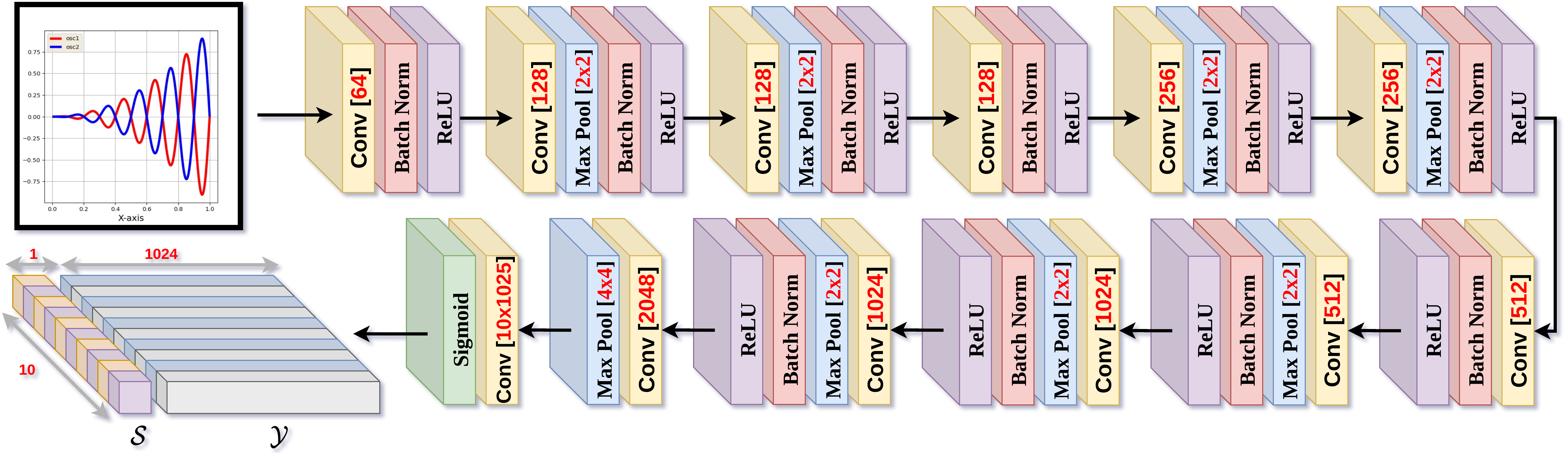
Given $\mathcal{I}$, we have two goals to accomplish: predicting the number of plots contained in the image and estimating $Y$ for each of these plots. We accomplish both of these goals simultaneously using a unified framework - APEX-Net. We first make an assumption about the maximum number of plots that can be contained in the image and denote it by $\hat{K}$. We choose $\hat{K}=10$, since most of the real world multiple plot images generally tend to contain less than $10$ plots. However, this is just a design parameter chosen for our network and is not a limitation of our framework. In order to accommodate images with higher number of plots, $\hat{K}$ can be increased. In our unified framework, given an image $\mathcal{I}$, our network produces two outputs $\mathcal{Y}$ and $\mathcal{S}$, where, $\mathcal{Y}=(Y_{1},Y_{2},\cdots,Y_{\hat{K}})$ and $\mathcal{S}=(s_{1},s_{2},\cdots,s_{\hat{K}})$. Here, $Y_{i}$ and $s_{i}$ denote the estimated y-coordinates and the confidence score of the $i^{th}$ predicted plot, respectively. The confidence score $s_{i}$ is a real value between $0$ and $1$, which denotes the probability of the $i^{th}$ predicted plot actually being present in the image. During inference, we only select those plots whose score is greater than $0.5$ and discard the rest.

Given an input image $\mathcal{I}$ of size $m\times n$, we first resize the image to a fixed size of $512\times 512$. We then pass the image through a sequence of blocks as depicted in Figure 1. Each block consists of a convolution layer, a batch normalization layer, and an activation function. The last block uses the sigmoid activation function to scale the values between $0$ and $1$. Apart from that, all the other blocks use ReLU (Rectified Linear Unit) as the activation function. Most of the blocks contain a max-pooling layer, which helps in progressively reducing the size of the feature maps. The network outputs $\mathcal{Y}$ and $\mathcal{S}$, which are tensors of size $10\times 1024$ and $10\times 1$, respectively.

Let $(\mathcal{I},\mathcal{Y}^{gt})$ be an example from the training dataset, where $\mathcal{Y}^{gt}=(Y^{gt}_{1},Y^{gt}_{2},\cdots,Y^{gt}_{K})$ is a tensor of size $K\times N$ denoting the y-coordinates of the ground-truth plot data. $K$ denotes the number of plots contained in $\mathcal{I}$ and $N=1024$. Let $\mathcal{Y}=(Y_{1},Y_{2},\cdots,Y_{\hat{K}})$ and $\mathcal{S}=(s_{1},s_{2},\cdots,s_{\hat{K}})$ be the output obtained after passing $\mathcal{I}$ through the network. The network is trained using two loss functions $\mathcal{L}_{plot}$ and $\mathcal{L}_{score}$ jointly, defined in Equation 1 and 2, respectively, where, $\left\lVert\cdot\right\rVert_{2}$ denotes the $\ell_{2}$ norm and $\chi_{A}$ is the characteristic function of $A$, where $A$ is given by Equation 3

The intuition behind using these loss functions is as follows: To each of the $K$ ground-truth plot, we assign the closest amongst the $\hat{K}$ predicted plot. To facilitate the extraction of accurate raw plot data, we minimize the distance between the obtained closest pairs. Further, if a predicted plot gets assigned to a ground-truth plot, we would prefer its score to be close to $1$ and $0$ otherwise.

Absence of deep learning methods for plot extraction prevents us from performing a detailed metric comparison. However, we mention the metric scores that our framework attains, which would serve as a baseline for other future works in this direction. Table 1 demonstrates the performance of our network on the test set of APEX-1M dataset. $\mathcal{E}_{plot}$ represents the plot loss $\mathcal{L}_{plot}$ (described in Equation 1) averaged over the entire test set. $\mathcal{E}_{count}$ denotes the relative count error averaged over the entire test set, where relative count error for a single example is given by $\frac{|K-\hat{K}|}{K}$. Visual results of our network on an example from the test set is shown in Figure 2(a). Results on unseen data, which are not a part of the APEX-1M dataset, are shown in Figure 2(b) and 2(c). We develop a GUI tool for providing the community with an easy to use plot extractor. Snippets of tool are shown in Figure 2(d) and 2(e).

References

- [1] Ankit Rohatgi, “Webplotdigitizer: Version 4.3,” 2020, Available at https://automeris.io/WebPlotDigitizer, Accessed on October 20, 2020.
- [2] Jiro Doke, “Grabit,” 2020, Available at https://www.mathworks.com/matlabcentral/fileexchange/7173-grabit, Accessed on October 20, 2020.
- [3] “Digitizeit,” Available at https://www.digitizeit.de/, Accessed on October 20, 2020.
- [4] “Getdatagraphdigitizer,” Available at http://getdata-graph-digitizer.com/index.php, Accessed on October 20, 2020.
- [5] “Plotdigitizer,” Available at http://plotdigitizer.sourceforge.net/, Accessed on October 20, 2020.
- [6] Mark Mitchell, Baurzhan Muftakhidinov, Tobias Winchen, et al., “Engauge digitizer software,” Webpage: http://markummitchell. github. io/engauge-digitizer. Accessed on October 20, 2020, vol. 11, 2017.
- [7] Peter Uwer, “Easyndata: A simple tool to extract numerical values from published plots,” arXiv preprint arXiv:0710.2896, 2007, Accessed on October 20, 2020.
- [8] “Quintessa graph grabber,” Available at https://www.quintessa.org/software/downloads-and-demos/graph-grabber-2.0.2, Accessed on October 20, 2020.
- [9] “Graph digitizer comparison – 16 ways to digitize your data,” Available at http://www.ifsc.usp.br/~lavfis/images/dados/digitalizarGrafico.pdf, Accessed on October 20, 2020.
- [10] Alex Krizhevsky, Ilya Sutskever, and Geoffrey E Hinton, “Imagenet classification with deep convolutional neural networks,” in Advances in neural information processing systems, 2012, pp. 1097–1105.
- [11] Ross Girshick, Jeff Donahue, Trevor Darrell, and Jitendra Malik, “Rich feature hierarchies for accurate object detection and semantic segmentation,” in Proceedings of the IEEE conference on computer vision and pattern recognition, 2014, pp. 580–587.
- [12] Jonathan Long, Evan Shelhamer, and Trevor Darrell, “Fully convolutional networks for semantic segmentation,” in Proceedings of the IEEE conference on computer vision and pattern recognition, 2015, pp. 3431–3440.
- [13] Ian Goodfellow, Jean Pouget-Abadie, Mehdi Mirza, Bing Xu, David Warde-Farley, Sherjil Ozair, Aaron Courville, and Yoshua Bengio, “Generative adversarial nets,” in Advances in neural information processing systems, 2014, pp. 2672–2680.
- [14] Shaoqing Ren, Kaiming He, Ross Girshick, and Jian Sun, “Faster r-cnn: Towards real-time object detection with region proposal networks,” in Advances in neural information processing systems, 2015, pp. 91–99.
- [15] Alexey Bochkovskiy, Chien-Yao Wang, and Hong-Yuan Mark Liao, “Yolov4: Optimal speed and accuracy of object detection,” arXiv preprint arXiv:2004.10934, 2020.
- [16] John D Hunter, “Matplotlib: A 2d graphics environment,” Computing in science & engineering, vol. 9, no. 3, pp. 90–95, 2007.