Efficient Semi-Implicit Variational Inference

Vincent Moens Affiliation: Huawei R&D UK Email: vincent.moens@huawei.com Hang Ren Affiliation: Huawei R&D UK Email: hang.ren1@huawei.com Alexandre Maraval Affiliation: Huawei R&D UK Email: alexandre.maravel@huawei.com Rasul Tutunov Affiliation: Huawei R&D UK Email: rasul.tutunov@huawei.com Jun Wang Affiliation: Huawei R&D UK Affiliation: University College London Email: w.j@huawei.com Haitham Ammar Thanks: Honorary position at UCL. Affiliation: Huawei R&D UK Affiliation: University College London Email: haitham.ammar@huawei.com

Abstract

In this paper, we propose CI-VI an efficient and scalable solver for semi-implicit variational inference (SIVI). Our method, first, maps SIVI’s evidence lower bound (ELBO) to a form involving a nonlinear functional nesting of expected values and then develops a rigorous optimiser capable of correctly handling bias inherent to nonlinear nested expectations using an extrapolation-smoothing mechanism coupled with gradient sketching. Our theoretical results demonstrate convergence to a stationary point of the ELBO in general non-convex settings typically arising when using deep network models and an order of $\mathcal{O}(t^{-\nicefrac{{4}}{{5}}})$ gradient-bias-vanishing rate. We believe these results generalise beyond the specific nesting arising from SIVI to other forms. Finally, in a set of experiments, we demonstrate the effectiveness of our algorithm in approximating complex posteriors on various data-sets including those from natural language processing.

1 Introduction

Variational Inference (VI) is an approximate Bayesian inference framework that recasts reasoning about latent variable models as an instance of numerical optimisation [15, 34]. This is achieved by positing a class of variational distributions and optimising an evidence lower-bound (ELBO) that involves log-joint densities rather than intractable posteriors. Classical VI introduces simplifying assumptions (e.g., mean-field and/or conditional conjugacy) to allow for tractable optimisation leading to algorithms that ascend to a stationary point of the ELBO [3, 15]. Though successful in many applications [21, 40, 49], such assumptions, unfortunately, restrict “representation-power” and thus, lead to models that underestimate the variance of the posterior.

Realising this problem, numerous frameworks aiming at expanding expressiveness of variational families have been proposed. Works in [10, 11, 12, 13, 15, 24, 31, 33, 34, 37, 38], for instance, relax mean-field assumptions and attempt to restore some dependencies in variational distributions but still require analytical probability density functions. Others in [14, 22, 25, 35, 38], moreover, introduce implicit models by sampling noise vectors and propagating these through deep networks [36]. These techniques do lead to distributions that are implicit but render computing log-variational densities and their gradients intractable. For this reason, authors resort to density ratio estimation; a methodology hard-to-scale and stabilise in high-dimensional settings.

To avoid density ratio estimation, recent work in [46] proposed semi-implicit variational inference (SIVI) as a hierarchical framework that obtains variational distributions through a mixing parameter accompanied by known-noise priors [36]. Exploiting this definition, original SIVI optimises a sequence of lower bounds that asymptotically converge to the original ELBO. Rather than focusing on approximate lower (upper) bounds, an unbiased estimator of the exact gradient of SIVI’s ELBO has been newly achieved [36] through a Hamiltonian Monte-Carlo simulator that draws samples from a reverse conditional acquiring state-of-the-art status. Though achieving better results than previous works, unbiased estimators based on Markov Chain Monte Carlo (MCMC) easily become computationally expensive in high-dimensional regimes. Hence, an efficient solver for models supporting semi-implicit variational family distributions, largely, remains an open problem to which we contribute in this paper.

Tackling the above problem, we present CI-VI, an efficient semi-implicit solver with rigorous theoretical guarantees capable of scaling to high-dimensional scenarios. Our method first maps the ELBO in SIVI to a nonlinear nested expectation (or compositional) form¹¹ 1 Please notice the decoupling between the inner and outer functions $f_{\nu}(\cdot)$ and $g_{\omega}(\cdot)$ . This requires us to further analyse SIVI’s ELBO; see Section 2.3., i.e., $\mathbb{E}_{\nu}[f_{\nu}\left(\mathbb{E}_{\omega}[\bm{g}_{\omega}(\bm{\theta})]\right)]$ with $\nu$ and $\omega$ being random variables²² 2 Please note we do not assume any independence between $\nu$ and $\omega$ , $f_{\nu}:\mathbb{R}^{n}\to\mathbb{R}$ , $\bm{g}_{w}:\mathbb{R}^{p}\to\mathbb{R}^{n}$ are smooth, not necessarily convex functions, and $\bm{\theta}$ the optimisation parameter – and then devises an algorithm capable of handling the bias resulting from the non-linear composition of $\mathbb{E}_{\omega}[\cdot]$ and $\mathbb{E}_{\nu}[\cdot]$ through $f_{\nu}(\cdot)$ . To do so, we introduce an extrapolation-smoothing step to an ADAM-like [18, 41] solver and, in turn, show vanishing gradient bias in the order of $\mathcal{O}(t^{-\nicefrac{{4}}{{5}}})$ ultimately enabling convergence to a stationary point. Our resulting algorithm shares similarities to recent work from [41] but unlocks novel theoretical results analysing gradient-bias terms. Though similar in spirit to [41], we realise that the original version presented in Algorithm 1 fails to scale to high-dimensions due to the need of computing large matrix-vector products (see Gradients’ instructions in Algorithm 1). Rectifying this problem, we lastly anchor a gradient-sketching mechanism allowing for batched matrix-vector products, and, further, study the theoretical outcomes of such a combination. Finally, we conduct an in-depth empirical study demonstrating that CI-VI outperforms other algorithms from SIVI, nested Monte-Carlo [30], and compositional optimisation [41, 44] literature.

2 Compositional implicit variational inference (CI-VI):

In this section, we demonstrate the connection between semi-implicit variational inference and compositional stochastic optimisation³³ 3 We use compositional and nested stochastic optimisation interchangeably.. We, first, present the semi-implicit inference framework as detailed in [36, 46], and then link to compositional optimisation in Section 2.2. We, finally, feature an efficient adaptive solver and provide its relevant theoretical guarantees in Section 2.3.

2.1 Semi-implicit variational inference

To approximate the posterior $p(\bm{z}|\bm{x})$ of a probabilistic model $p(\bm{x},\bm{z})$ , we define a semi-implicit variational distribution $q_{\bm{\theta}}(\bm{z})$ in a hierarchical fashion using a mixing parameter as introduced in [36]:

\bm{\epsilon}\sim q(\bm{\epsilon}),\ \ \ \ \bm{z}\sim q_{\bm{\theta}}(\bm{z}|\bm{\epsilon})\ \ \ \ \implies\ \ \ \ q_{\bm{\theta}}(\bm{z})=\underbrace{\int q_{\bm{\theta}}(\bm{z}|\bm{\epsilon})q(\bm{\epsilon})d\bm{\epsilon}}_{\text{intractable}}.

(1)

Equation 1 reveals the reason behind $q_{\bm{\theta}}(\bm{z})$ being implicit as we can obtain latent variable samples through $\bm{\epsilon}$ but can not (tractably) compute the integral especially when using deep networks in representing $q_{\bm{\theta}}(\bm{z}|\bm{\epsilon})$ . In this work, we impose two standard assumptions on the nature of the variational distribution as previously explained in [36, 46]. The first assumes that $q_{\bm{\theta}}(\bm{z}|\bm{\epsilon})$ is reparameterisable. That is, to obtain samples from $\bm{z}\sim q_{\bm{\theta}}(\bm{z}|\bm{\epsilon})$ , one can draw an auxiliary variable $\bm{u}$ and then set $\bm{z}$ as a deterministic function $h_{\bm{\theta}}(\cdot)$ of the sampled $\bm{u}$ i.e., $\bm{u}\sim q(\bm{u}),\ \bm{z}=h_{\bm{\theta}}(\bm{u};\bm{\epsilon})\ \equiv\ \bm{z}\sim q_{\bm{\theta}}(\bm{z}|\bm{\epsilon})$ . The second, moreover, assumes that we can evaluate the log-density of the conditional i.e., $\log q_{\bm{\theta}}(\bm{z}|\bm{\epsilon})$ as well as its gradient. As noted in [36], such an assumption is not strong in that it holds for many reparameterisable distributions, e.g., Gaussian, Laplace, exponential, and many others. Analogous to standard variational inference, model parameters are fit by minimising the negate of an evidence-lower (ELBO) bound that can be derived as follows:

\log p(\bm{x})=\log\int\frac{q_{\bm{\theta}}(\bm{z})}{q_{\bm{\theta}}(\bm{z})}p(\bm{x},\bm{z})d\bm{z}\geq\int q_{\bm{\theta}}(\bm{z})\log\left[\frac{p(\bm{x},\bm{z})}{q_{\bm{\theta}}(\bm{z})}\right]d\bm{z}=\mathbb{E}_{q_{\bm{\theta}}(\bm{z})}\left[\log\frac{p(\bm{x},\bm{z})}{q_{\bm{\theta}}(\bm{z})}\right].

(2)

Contrary to classical VI that assumes tractable expectations, SIVI introduces additional intractability (e.g., in the entropy term) due to the implicit nature of the variational distribution defined in Equation 1. To tackle such intractability, recently the authors in [36] proposed writing the gradient of the entropy term as an expectation and following an MCMC sampler [42], e.g., Hamiltonian Monte Carlo [2] to estimate the gradient of the ELBO. MCMC methods, however, are known to be computationally expensive and can exhibit high variance as they assume no model – see Section 3 for a detailed comparison. Rather than following MCMC, in this paper we contribute by showing that the semi-implicit ELBO can be written as an instance of compositional optimisation and devise an adaptive and efficient solver with rigorous theoretical guarantees.

2.2 SIVI in a compositional nested form

In this section, we present a novel connection mapping implicit variational inference to compositional stochastic optimisation, paving-the-way for an efficient and scalable solver that we later develop in Section 2.3. To do so, we start by plugging-in the variational distribution from Equation 1 in the inner-part of the ELBO (i.e., Equation 2) to get: $\log p(\bm{x})\geq\mathbb{E}_{\bm{z}\sim q_{\bm{\theta}}(\bm{z})}\left[\log\frac{p(\bm{x},\bm{z})}{q_{\bm{\theta}}(\bm{z})}\right]=\mathbb{E}_{\bm{z}\sim q_{\bm{\theta}}(\bm{z})}\left[\log\frac{p(\bm{x},\bm{z})}{\mathbb{E}_{\bm{\hat{\epsilon}}\sim q(\bm{\epsilon})}[q_{\bm{\theta}}(\bm{z}|\bm{\hat{\epsilon}})]}\right]$ , where we used $\bm{\hat{\epsilon}}$ to denote an inner-random variable also sampled according to $q(\bm{\epsilon})$ . As noted earlier, we assume that the conditional $q_{\bm{\theta}}(\bm{z}|\bm{\epsilon})$ is reparameterisable through an auxiliary variable $\bm{u}$ and a deterministic function $h_{\bm{\theta}}(\bm{u};\bm{\epsilon})$ with $\bm{\epsilon}\sim q(\bm{\epsilon})$ but independent from $\bm{\hat{\epsilon}}$ . Rather than reparametrising both inner and outer expectations, we only reparameterise the outer expectation leading us to:

	$\displaystyle\mathbb{E}_{\bm{z}\sim q_{\bm{\theta}}(\bm{z})}\left[\log\frac{p(\bm{x},\bm{z})}{\mathbb{E}_{\bm{\hat{\epsilon}}\sim q(\bm{\epsilon})}[q_{\bm{\theta}}(\bm{z}\|\bm{\hat{\epsilon}})]}\right]$	$\displaystyle=\mathbb{E}_{\bm{u}\sim q(\bm{u}),\bm{\epsilon}\sim q(\bm{\epsilon})}\left[\log\frac{p(\bm{x}\|h_{\bm{\theta}}(\bm{u};\bm{\epsilon}))p(h_{\bm{\theta}}(\bm{u};\bm{\epsilon}))}{\mathbb{E}_{\bm{\hat{\epsilon}}\sim q(\bm{\epsilon})}[q_{\bm{\theta}}\left(h_{\bm{\theta}}(\bm{u};\bm{\epsilon})\|\bm{\hat{\epsilon}}\right)]}\right]$
		(reparam.)

Remembering that in variational inference one minimises the negate of the ELBO, we can further write:

	$\displaystyle-\mathbb{E}_{\bm{u}\sim q(\bm{u}),\bm{\epsilon}\sim q(\bm{\epsilon})}\left[\log\frac{p(\bm{x}\|h_{\bm{\theta}}(\bm{u};\bm{\epsilon}))p(h_{\bm{\theta}}(\bm{u};\bm{\epsilon}))}{\mathbb{E}_{\bm{\hat{\epsilon}}}[q_{\bm{\theta}}\left(h_{\bm{\theta}}(\bm{u};\bm{\epsilon})\|\bm{\hat{\epsilon}}\right)]}\right]$	$\displaystyle=\mathbb{E}_{q(\bm{u}),q(\bm{\epsilon})}\left[\log\frac{\mathbb{E}_{\bm{\hat{\epsilon}}\sim q(\bm{\epsilon})}[q_{\bm{\theta}}\left(h_{\bm{\theta}}(\bm{u};\bm{\epsilon})\|\bm{\hat{\epsilon}}\right)]}{p(\bm{x}\|h_{\bm{\theta}}(\bm{u};\bm{\epsilon}))p(h_{\bm{\theta}}(\bm{u};\bm{\epsilon}))}\right]$
		$\displaystyle=\mathbb{E}_{\bm{\mu}\sim q(\bm{\mu})}[\log\mathbb{E}_{\bm{\hat{\epsilon}}}[\mathcal{J}_{\bm{\mu},\bm{\hat{\epsilon}}}(\bm{\theta})]],$

where we used $\bm{\mu}=\{\bm{u},\bm{\epsilon}\}$ to concatenate outer random variables with $q(\bm{\mu})=q(\bm{u},\bm{\epsilon})=q(\bm{u})q(\bm{\epsilon})$ . Hence, the optimisation problem involved in SIVI can be written as: $\min_{\bm{\theta}}\mathbb{E}_{\bm{\mu}}[\log\mathbb{E}_{\bm{\hat{\epsilon}}}[\mathcal{J}_{\bm{\mu},\bm{\hat{\epsilon}}}(\bm{\theta})]]$ . Superficially, the aforementioned problem looks compositional in nature due to the non-linear (through the logarithm) nesting of both expectations. It is worth emphasizing, however, that the standard nested form introduced in Section 1 assumes an inherent decoupling between the inner and outer expectations, i.e., $\mathbb{E}_{\nu}[f_{\nu}\left(\mathbb{E}_{\omega}[\bm{g}_{\omega}(\bm{\theta})]\right)]$ . In light of this realisation, we now introduce a formalisation capable of achieving this decoupling. To do so, we consider a pool of $n$ - $\bm{\mu}$ samples distributed according to $q(\bm{\mu})$ : $\text{Pool}=\{\bm{\mu}_{i}=\left\langle\bm{u}_{i},\bm{\epsilon}_{i}\right\rangle\}_{i=1}^{n}$ . Now, we define a vector-valued function, $\bm{g}_{\bm{\hat{\epsilon}}}(\bm{\theta})$ , of size $n$ corresponding to the evaluations of $\mathcal{J}_{\bm{\mu},\bm{\hat{\epsilon}}}(\bm{\theta})$ on each of the samples from the pool, i.e., $\forall j\in[1,n]$ we have: $\bm{g}_{\bm{\hat{\epsilon}}}(\bm{\theta})=[\mathcal{J}_{\bm{\mu}_{1},\bm{\hat{\epsilon}}}(\bm{\theta}),\dots,\mathcal{J}_{\bm{\mu}_{n},\bm{\hat{\epsilon}}}(\bm{\theta})]^{\mathsf{T}},\ \text{with $\mathcal{J}_{\bm{\mu}_{j},\bm{\hat{\epsilon}}}(\bm{\theta})=\frac{q_{\bm{\theta}}\left(h_{\bm{\theta}}(\bm{u}_{j};\bm{\epsilon}_{j})|\bm{\hat{\epsilon}}\right)}{p(\bm{x}|h_{\bm{\theta}}(\bm{u}_{j};\bm{\epsilon}_{j}))p(h_{\bm{\theta}}(\bm{u}_{j};\bm{\epsilon}_{j}))}$.}$ To achieve the decoupling between inner an outer expectations, we allow $f_{\nu}(\bm{y})=[\log\bm{y}]^{\mathsf{T}}\bm{e}_{\nu}$ with $\bm{e}_{\nu}$ being the $\nu$ ’th basis vector in $\mathbb{R}^{n}$ , i.e., a vector of all zeros except a value of one in the $\nu$ ’th position. Sampling uniformly from the pool, we can finally write SIVI’s optimisation problem in a compositional form as:

\min_{\bm{\theta}}\mathbb{E}_{\nu\sim\text{Uniform}[1,n]}\left[f_{\nu}\left(\mathbb{E}_{\bm{\hat{\epsilon}}\sim q(\bm{\epsilon})}[\bm{g}_{\bm{\hat{\epsilon}}}(\bm{\theta})]\right)\right]\equiv\min_{\bm{\theta}}\mathcal{L}(\bm{\theta}),

(3)

with $f_{\nu}(\bm{y})=[\log\bm{y}]^{\mathsf{T}}\bm{e}_{\nu}$ and $\bm{g}_{\bm{\hat{\epsilon}}}(\bm{\theta})=[\mathcal{J}_{\bm{\mu}_{1},\bm{\hat{\epsilon}}}(\bm{\theta}),\dots,\mathcal{J}_{\bm{\mu}_{n},\bm{\hat{\epsilon}}}(\bm{\theta})]^{\mathsf{T}}$ . Clearly, our problem becomes exact only when assuming an infinite number of samples, i.e., $n\rightarrow\infty$ . As such, one would naturally choose $n$ to be large-enough for a small variance estimator of the loss. This, in turn, adds complexity in designing a solver that now has to handle nested expectations and high-dimensional regimes. In the next section, we introduce such an algorithm through a novel combination of extrapolation-smoothing and gradient sketching mechanisms.

2.3 An adaptive solver

When designing a solver for the optimisation problem in Equation 3, we consider three essential criteria. First, we would like a simple-to-implement (i.e., single loop) yet effective and scalable algorithm. Second, we aim to have a bias-controlling procedure⁴⁴ 4 Here, it is to be understood that bias is due to estimating nonlinear nested expectations. and third, we need a rigorous and theoretically-grounded solver. When surveying optimisation literature, we realise that a promising direction is a first-order method as opposed to zero [9] or second-order [39] ones. Such a realisation is grounded in the fact that first-order methods only require gradient information, are typically simple to implement through a single-loop, and perform competitively in large-scale machine learning applications [6, 18, 26]. Among first-order methods, one can further categorise adaptive [6, 26, 48] and momentum-based [20, 28] algorithms. In spite of numerous theoretical developments [1, 7, 23], ADAM – an adaptive optimiser originally proposed in [18], and then theoretically grounded in [32, 47] – (arguably) retains state-of-the-art status. Therefore, following an adaptive-like update scheme to solving the problem in Equation 3 promises ease of implementation and scalability to real-world scenarios.

Though meeting two out of the three criteria above, a simple adaptation of standard optimisation techniques to a compositional problem of the form in Equation 3 is challenging due to the bias incurred from a naive Monte-Carlo sampling of non-linear nested expectations; see [30] for a detailed discussion. Of course, such a problem is not unique to this paper and has been previously studied in [30, 43]. Current methods, however, are either not-scalable to high-dimensional large-data problems [4, 27] (e.g., require full gradients -- over all data -- for variance reduction), or solve a relaxed version that presumes a finite sum empirical-risk-minimisation⁵⁵ 5 Please note that relaxed empirical-risk versions target a different problem all-together [43]. In other words, solving a finite-sum approximation does not guarantee convergence for the nested expectation problem presented in Equation 3. problem [30, 43]. To meet our requirements, we next present a novel solver that combines extrapolation-smoothing for bias-reduction and gradient-sketching for efficiency and scalability. It is worth noting that our optimiser shares similarities to the work by [41] but refines analysis to derive bias-handling results (Equation 5) and introduces additional constructs (e.g., gradient-sketching mechanisms). Such additions require new proof foundations and re-derivations that we present in the appendix for completeness.

Algorithmic development

We aim to offer an adaptive algorithm that exhibits similar (theoretical and practical) performance guarantees to ADAM but that is also capable of correctly handling the bias inherent to the problem in Equation 2. To do so, we introduce an update scheme that resembles ADAM but incorporates auxiliary variables that are updated in a subsequent step. Being at an iteration $t$ , our algorithm first executes the following updates:

		$\displaystyle\bm{m}_{t}=\gamma_{t}^{(1)}\bm{m}_{t-1}+\left(1-\gamma_{t}^{(1)}\right)\overline{\nabla\mathcal{L}(\bm{\theta}_{t})}\ ,\ \bm{v}_{t}=\gamma_{t}^{(2)}\bm{v}_{t-1}+\left(1-\gamma_{t}^{(2)}\right)[\overline{\nabla\mathcal{L}(\bm{\theta}_{t})}]^{2}$
		$\displaystyle\hskip 110.99927pt\rightsquigarrow\bm{\theta}_{t+1}=\bm{\theta}_{t}-\alpha_{t}\frac{\bm{m}_{t}}{\sqrt{\bm{v}_{t}}+\xi},$
		with $\alpha_{t}$ being a learning rate, $\xi\in\mathbb{R}_{>0}$ , $\gamma_{t}^{(1)}$ and $\gamma_{t}^{(2)}$ denoting hyper-parameters.

Assuming the availability of sub-sampled gradients of the loss (i.e., $\overline{\nabla\mathcal{L}(\bm{\theta}_{t})}$ ), the above set of instructions simply performs an ADAM-like update on the model’s free parameters⁶⁶ 6 It is worth noting that later in our theoretical analysis we provide a rigorous scheme for tuning all hyper-parameters. We also follow such a schedule in our experiments. $\bm{\theta}$ starting from an initialisation for $\bm{m}_{t}$ and $\bm{v}_{t}$ . The problem, however, arises when aiming to acquire unbiased gradients of the objective in Equation 3 [30, 36, 46]. To illustrate this, consider computing the actual gradient of $\mathcal{L}(\bm{\theta})$ at some iteration $t$ . This can be written as: $\nabla\mathcal{L}(\bm{\theta}_{t})=\mathbb{E}_{\bm{\hat{\epsilon}}}[\nabla\bm{g}_{\bm{\hat{\epsilon}}}(\bm{\theta}_{t})]^{\mathsf{T}}\mathbb{E}_{\nu}[\nabla f_{\nu}\left(\mathbb{E}_{\bm{\hat{\epsilon}}}[\bm{g}_{\bm{{\hat{\epsilon}}}}(\bm{\theta}_{t})]\right)]$ . It is clear that one can easily implement a Monte-Carlo estimator of the first part of the gradient, i.e., $\mathbb{E}_{\bm{\hat{\epsilon}}}[\nabla\bm{g}_{\bm{\hat{\epsilon}}}(\bm{\theta}_{t})]$ . The second term, on the other hand, is much harder to estimate due to its nested nature:

\mathbb{E}_{\nu}[\nabla f_{\nu}\left(\mathbb{E}_{\bm{\hat{\epsilon}}}[\bm{g}_{\bm{{\epsilon}}_{2}}(\bm{\theta}_{t})]\right)]=\mathbb{E}_{\nu}\left[\frac{1}{\left(\mathbb{E}_{\bm{\hat{\epsilon}}}[\bm{g}_{\bm{\hat{\epsilon}}}(\bm{\theta}_{t})]\right)_{\nu}}\right],\ \ \text{where $(\bm{v})_{\nu}$ denotes the $\nu^{th}$ component of $\bm{v}$.}

(4)

Of course, a simple Monte-Carlo estimator⁷⁷ 7 We mean by a simple estimator the following: $\mathbb{E}_{\nu}\left[\frac{1}{\left(\mathbb{E}_{\bm{\hat{\epsilon}}}[\bm{g}_{\bm{\hat{\epsilon}}}(\bm{\theta}_{t})]\right)_{\nu}}\right]\approx\frac{1}{N}\sum_{i=1}^{N}\left[\frac{1}{\left(\frac{1}{M}\sum_{j=1}^{M}\bm{g}_{j}(\bm{\theta}_{t})\right)_{i}}\right]$ . of the gradient’s second part is biased. Our methodology in tackling this challenge is to find an “unbiased” approximation with properties allowing us to control such a bias at appropriate rates. To do so, we follow an extrapolation-smoothing scheme [41, 43, 44] originally established in time series [45] and differential equations literature [17]. These methods introduce a two-step procedure to approximate an unknown quantity, e.g., $\mathbb{E}_{\nu}[\nabla f_{\nu}\left(\mathbb{E}_{\bm{\hat{\epsilon}}}[\bm{g}_{\bm{{\hat{\epsilon}}}}(\bm{\theta}_{t})]\right)]$ in our case. In the first step, a linear extrapolation query vector, $\bm{z}$ , is computed while in the second, a smoothed average is evaluated around the extrapolated $\bm{z}$ . Precisely, given two model parameter updates $\bm{\theta}_{t}$ and $\bm{\theta}_{t+1}$ we execute the following:

		$\displaystyle\bm{z}_{t+1}=\underbrace{\left(1-\nicefrac{{1}}{{\beta}}_{t}\right)\bm{\theta}_{t}+\nicefrac{{1}}{{\beta_{t}}}\bm{\theta}_{t+1}}_{\text{Extrapolation}}\ \ \text{and}\ \ \bm{y}_{t+1}=\underbrace{(1-\beta_{t})\bm{y}_{t}+\beta_{t}\overline{\bm{g}_{t}(\bm{z}_{t+1})}}_{\text{Smoothing}},$
		$\displaystyle\text{with $\beta_{t}$ being a free parameter, and $\overline{\bm{g}_{t}(\bm{z}_{t+1})}$ is a sampled estimator of $\mathbb{E}_{\bm{\hat{\epsilon}}}[{\bm{g}}_{\bm{\hat{\epsilon}}}\left(\bm{z}_{t+1}\right)]$}.$

Simply, the smoothing step is attempting to track $\mathbb{E}_{\bm{\hat{\epsilon}}}[{\bm{g}}_{\bm{\hat{\epsilon}}}\left(\bm{z}_{t+1}\right)]$ which can then be substituted in Equation 4 to approximate the second term of the gradient. Interestingly, we evaluate this smoothing step around a linearly extrapolated vector $\bm{z}_{t+1}$ and not only on the updated model parameters $\bm{\theta}_{t+1}$ . Though an evaluation around $\bm{\theta}_{t+1}$ can guarantee convergence [43], we demonstrate that following the above extrapolation scheme leads to faster convergence rates by enabling a better control of the bias. Informally, we can, under further technical consideration, demonstrate that the difference between true and sub-sampled gradients abides by:

\mathbb{E}_{\text{total}}[||\nabla\mathcal{L}(\bm{\theta}_{t})-\overline{\nabla\bm{g}_{t}(\bm{\theta}_{t})}^{\mathsf{T}}\overline{\nabla f_{t}(\bm{y}_{t})}||_{2}^{2}]\approx\mathcal{O}(t^{-\nicefrac{{4}}{{5}}}),

(5)

where $\overline{\nabla\bm{g}_{t}(\bm{\theta}_{t})}$ and $\overline{\nabla f_{t}(\bm{y}_{t})}$ denote estimate gradients of the functions $\bm{g}_{\bm{\hat{\epsilon}}}(\cdot)$ and $f_{\nu}(\cdot)$ , and $\mathbb{E}_{\text{total}}[\cdot]$ the expectation under all incurred randomness in the algorithm. Importantly, the result in Equation 5 shows that the bias in our gradient estimator vanishes with an increased number of iterations. This, in turn, allows us to prove convergence of the resulting algorithm as studied in Section 2.3. We now introduce the complete algorithm combining both of the above primary and auxiliary steps. To that end, we assume a schedule of learning rates $\eta\text{-schedule}=\{\langle\alpha_{t},\beta_{t},\gamma^{(1)}_{t},\gamma_{t}^{(2)}\rangle\}_{t=1}^{T}$ , and a time-varying set of batch-sizes $K\text{-size}=\{\langle K_{t}^{(1)},K_{t}^{(2)},K_{t}^{(3)}\rangle\}$ needed to mini-batch $\nabla f_{\nu}(\cdot)$ , $\nabla\bm{g}_{\bm{\hat{\epsilon}}}(\cdot)$ , and $\mathbb{E}_{\bm{\hat{\epsilon}}}[\bm{g}_{\bm{\hat{\epsilon}}}(\cdot)]$ respectively. Our computations are achieved through two oracles that can return gradients and function values when needed⁸⁸ 8 Please note that in Section 2.3 we provide explicit schedules for each of the hyper-parameters introduced.:

	$\displaystyle\text{Oracle}_{f}\left(\bm{y}_{t},K_{t}^{(1)}\right)$	$\displaystyle=\{\langle\nu_{t_{i}},\nabla f_{\nu_{t_{i}}}(\bm{y}_{t})\rangle\}_{i=1}^{K_{t}^{(1)}},\ \ \text{with $\{\nu_{t_{i}}\}_{i=1}^{K_{t}^{(1)}}$ being i.i.d.}$
	$\displaystyle\text{Oracle}_{g}\left(\bm{z}_{t},K_{t}^{(2)}\right)$	$\displaystyle=\{\langle\bm{\hat{\epsilon}}_{t_{i}},\bm{g}_{\bm{\hat{\epsilon}}_{t_{i}}}(\bm{z}_{t}),\nabla\bm{g}_{\bm{\hat{\epsilon}}_{t_{i}}}(\bm{z}_{t})\rangle\}_{i=1}^{K_{t}^{(2)}},\ \ \text{with $\{\bm{\hat{\epsilon}}_{t_{i}}\}_{i=1}^{K_{t}^{(2)}}$ also i.i.d.}$

In addition, we define $\delta\in(0,1)$ used to measure solution accuracy and a small positive constant $\xi$ for numerical stability. The overall procedure is practical requiring only one implementation loop and is summarised in Algorithm 1. It operates in three main steps. In the first, sub-sampled gradients are computed by calling $\text{Oracle}_{f}(\cdot)$ and $\text{Oracle}_{g}(\cdot)$ . When estimated, the second step computes primary updates leading to improved model parameters $\bm{\theta}_{t+1}$ . Given $\bm{\theta}_{t}$ and $\bm{\theta}_{t+1}$ , the third step executes extrapolation-smoothing to update an estimate of $\mathbb{E}_{\bm{\hat{\epsilon}}}[\bm{g}_{\bm{\hat{\epsilon}}}(\cdot)]$ guaranteeing vanishing bias with increased iterations. It is to be noted that the smoothing step requires an additional call to $\text{Oracle}_{g}(\cdot)$ to sample $\overline{\bm{g}_{t}(\bm{z}_{t+1})}$ . The updated smoothed variable $\bm{y}_{t+1}$ is then used in subsequent iterations where the overall process repeats.

Algorithm 1 CI-VI: Compositional Implicit Variational Inference

Inputs: Initial variable

\bm{\theta}_{1}

\delta\in(0,1)

\xi

T=\mathcal{O}(\delta^{-\nicefrac{{5}}{{4}}})

\eta\text{-schedule}

and

K\text{-size}

Initialisation: Initialise

\bm{z}_{1}=\bm{\theta}_{1}

\bm{y}_{1}=\bm{0}

, and

\bm{m}_{0}=\bm{v}_{0}=0

for

t=1

T

do:

Compute sub-sampled gradients by calling oracles:

\triangleright\ \text{Gradients}

	$\displaystyle\overline{\nabla f_{t}(\bm{y}_{t})}$	$\displaystyle=\nicefrac{{1}}{{K_{t}^{(1)}}}\sum_{i=1}^{K_{t}^{(1)}}\nabla f_{\nu_{t_{i}}}(\bm{y}_{t})$		$\displaystyle\raisebox{-24.0pt}[1.0pt][1.0pt]{ \text{$\implies\overline{\nabla\mathcal{L}(\bm{\theta}_{t})}=\overline{\nabla\bm{g}_{t}(\bm{\theta}_{t})}^{\mathsf{T}}\overline{\nabla f_{t}(\bm{y}_{t})}$} }$
	$\displaystyle\overline{\nabla\bm{g}_{t}(\bm{\theta}_{t})}$	$\displaystyle=\nicefrac{{1}}{{K_{t}^{(2)}}}\sum_{j=1}^{K_{t}^{(2)}}\nabla\bm{g}_{\bm{\hat{\epsilon}}_{t_{j}}}(\bm{\theta}_{t})$

Perform the following primary updates:

\triangleright\ \text{Primary Update}

	$\displaystyle\bm{m}_{t}$	$\displaystyle=\gamma_{t}^{(1)}\bm{m}_{t-1}+\left(1-\gamma_{t}^{(1)}\right)\color[rgb]{1,0.5,0}\overline{\nabla\mathcal{L}(\bm{\theta}_{t})}$		$\displaystyle\raisebox{-7.20007pt}[1.0pt][1.0pt]{ \text{$\implies\bm{\theta}_{t+1}=\bm{\theta}_{t}-\alpha_{t}\frac{\bm{m}_{t}}{\sqrt{\bm{v}_{t}}+\xi}$} }$
	$\displaystyle\bm{v}_{t}$	$\displaystyle=\gamma_{t}^{(2)}\bm{v}_{t-1}+\left(1-\gamma_{t}^{(2)}\right)\color[rgb]{1,0.5,0}[\overline{\nabla\mathcal{L}(\bm{\theta}_{t})}]^{2}$

Perform the following auxiliary updates:

\triangleright\ \text{Auxiliary Update}

\bm{z}_{t+1}=\underbrace{\left(1-\nicefrac{{1}}{{\beta}}_{t}\right)\bm{\theta}_{t}+\nicefrac{{1}}{{\beta_{t}}}\bm{\theta}_{t+1}}_{\text{Extrapolation}}\ \ \text{and}\ \ \bm{y}_{t+1}=\underbrace{(1-\beta_{t})\bm{y}_{t}+\beta_{t}\overline{\bm{g}_{t}(\bm{z}_{t+1})}}_{\text{Smoothing}}

Output: Return solution as a uniform sample from

\left\{\bm{\theta}_{t}\right\}_{t=1}^{T}

On practicability

Algorithm 1, though successful, assumes an idealised setting in which computing products of gradient estimates is feasible. In most reasonably-sized problems, however, such products are prohibitively expensive due to the problem’s dimensionality and number of samples available (e.g., order of thousands). To remedy this problem, we next present a matrix-sketching mechanism (not introduced previously in both variational inference and compositional optimisation literature) from randomised linear algebra [5] enabling scalability. Here, we simply replace gradient computations (in orange) in Algorithm 1 with the set of instructions⁹⁹ 9 In Algorithm 2, we use $\bm{A}(:,k)$ to denote the $k^{th}$ column of some matrix $\bm{A}$ , and $\boldsymbol{b}(k)$ the $k^{th}$ component of a vector $\bm{b}$ . in Algorithm 2 that eases implementation in that it allows for randomised matrix-vector products which come-in handy in big-data problems. Rather than needing to sum overall entries in the corresponding product, we can now simply enable a batch-like version through sketching. Chiefly, as we show in Section 3, we can further specialise Algorithm 2 by accounting for the sparsity pattern of our gradients for improved adjustability to the SIVI setting.

Algorithm 2 Gradient-Sketching for Large-Scale SIVI

Inputs:

\text{Oracle}_{f}(\bm{y}_{t},K_{t}^{(1)})

\text{Oracle}_{g}(\bm{\theta}_{t},K_{t}^{(2)})

, #-samples

d_{t}\in[1,n]

Sample subset

S_{t}\subseteq[1,\ldots,n]

of size

d_{t}

, where

\mathbb{P}\text{r}(k\in S_{t})=\nicefrac{{1}}{{n}}

for all

k=1,\ldots,n

Return:

\overline{\nabla\mathcal{L}(\bm{\theta}_{t})}=\nicefrac{{1}}{{K^{(1)}_{t}}}\sum_{a=1}^{K^{(1)}_{t}}[\nicefrac{{q}}{{d_{t}}}\sum_{k\in S_{t}}\nabla\boldsymbol{g}_{\bm{\hat{\epsilon}}_{t_{a}}}^{\mathsf{T}}(\bm{\theta}_{t})(:,k)\nabla f_{\nu_{t_{a}}}(\boldsymbol{y}_{t})(k)]

Of course, sketching mechanisms can affect speeds of convergence due to additionally induced randomness. To gain insight into such phenomena, we next provide rigorous theoretical guarantees demonstrating convergence of the resulting algorithm (i.e., Algorithm 1 with Sketching for gradient computation) and quantifying oracle complexities.

Theoretical guarantees

We demonstrate that Algorithm 1 converges to a stationary point of the non-convex objective¹⁰¹⁰ 10 Non-convexity is abundant in our problem due to the usage of neural networks. In these scenarios, one aims at a stationary point as even assessing a local-minimum is NP-Hard [16]. in Equation 3. As is standard in optimisation literature, we provide our results in terms of the number of oracle calls needed to convergence¹¹¹¹ 11 Please note that analysing other metrics, e.g., generalisation bounds is an interesting avenue for future research.. Due to space constraints, we defer the proof to the appendix. Here, we provide the statement of the main theorem. Our main results are based on the following common assumptions:

Assumption 1.

We make the following assumptions¹²¹² 12 Please note that for additional clarity, our assumptions are further elaborated in the appendix.: 1) $\left|f_{\nu}(\bm{y})\right|\leq B_{f}$ , and $\left|\left|\nabla f_{\nu}(\bm{y})\right|\right|\leq M_{f}$ , for all $\bm{y}$ and $\nu$ ; 2) $f_{\nu}(\cdot)$ is $L_{f}$ -smooth, and $\bm{g}_{\bm{\hat{\epsilon}}}(\bm{x})$ is $M_{g}$ - Lipschitz continuous, and $L_{g}$ -smooth; 3) oracle sample-pairs are independent; and 4) oracles return unbiased gradient estimates with bounded variances.

Now, we present the main theorem analysing convergence and oracle complexities of Algorithm 1:

Theorem 1 (Convergence & Oracle Complexities).

Consider a parameter setup given by: $\alpha_{t}=\nicefrac{{C_{\alpha}}}{{t^{\frac{1}{5}}}},\beta_{t}=C_{\beta},K_{t}^{(1)}=C_{1}t^{\frac{4}{5}},K_{t}^{(2)}=C_{2}t^{\frac{4}{5}},K_{t}^{(3)}=C_{3}t^{\frac{4}{5}},\gamma_{t}^{(1)}=C_{\gamma}\mu^{t},\ \gamma_{2}^{(t)}=1-\nicefrac{{C_{\alpha}}}{{t^{\frac{2}{5}}}}(1-C_{\gamma}\mu^{t})^{2}$ , for some positive constants $C_{\alpha},C_{\beta},C_{1},C_{2},C_{3},C_{\gamma},\mu$ such that $C_{\beta}<1$ and $\mu\in(0,1)$ . For any $\delta\in(0,1)$ , Algorithm 1 running gradient-sketching (i.e., using Algorithm 2 to compute gradient products) with a sample-size $d_{t}=\mathcal{O}(1)$ outputs, in expectation, a $\delta$ -approximate first-order stationary point $\tilde{\bm{\bm{\theta}}}$ of $\mathcal{L}(\bm{\bm{\theta}})$ . That is: $\mathbb{E}_{\textrm{total}}[||\nabla\mathcal{L}(\tilde{\bm{\theta}})||_{2}^{2}]\leq\delta$ , with “total” representing all incurred randomness. Moreover, Algorithm 1 acquires $\tilde{\bm{\theta}}$ with an overall oracle complexity of the order $\mathcal{O}\left(\delta^{-\nicefrac{{9}}{{4}}}\right)$ .

3 Experiments and results

In this section, we present an empirical study demonstrating the effectiveness of CI-VI that we implement in PyTorch [29]. We benchmark on three broad tasks covering toy examples, Bayesian logistic regression and variational autoencoders. Of course, our derivations need to be specialised to each of these tasks. We provide such constructs in the appendix due to space constraints. We compare against standard semi-implicit variational inference algorithms (e.g., SIVI and UIVI) in addition to methods from nested Monte-Carlo [30] and compositional optimisation [43, 44]. To improve stability and computational efficiency, our implementation of CI-VI tracks log-gradients instead of $\overline{\nabla\mathcal{L}(\bm{\theta}_{t}})$ . Furthermore, due to the special structures of $f_{\nu}(\cdot)$ (e.g., logarithmic function) and $g_{\hat{\bm{\epsilon}}}$ , we can further improve gradient sketching by only (uniformly) sampling non-zero elements from $\nabla g_{\bm{\hat{\epsilon}}}(\cdot)$ rather than the whole $d_{t}$ -set $S_{t}$ in Algorithm 2. Due to space constraints, such adaptations in addition to exact experimental settings can be found in the appendix. We ran all experiments on a single NVIDIA GeForce RTX 2080 GPU. Crucially, CI-VI is highly efficient consuming 30 seconds for toy experiments and, at most, 1.5 hours for text modelling when using variational autoencoders.

Toy Experiments: In this set of experiments, we apply our method to minimise a KL-divergence between semi-implicit and ground truth distributions on two-modal, star, and banana as taken from [36].

Figure 1: Results demonstrating that CI-VI can approximate sophisticated distributions from [36]. Left: Two-Modal distribution, Middle: Star distribution, and Right: Banana distribution.

For all semi-implicit distributions, we chose $q(\bm{\epsilon})$ to be a multi-variate zero-mean identity-covariance-matrix Gaussian, i.e., $q(\bm{\epsilon})=\mathcal{N}(\bm{0},\bm{I}_{3\times 3})$ . The conditional distribution $q_{\bm{\theta}}(\bm{z}|\bm{\epsilon})$ , is also assumed Gaussian with a neural network (two layers 50 by 50 hidden units) parameterised mean and a parameterised diagonal covariance matrix, where $q_{\bm{\theta}}(\bm{z}|\epsilon)=\mathcal{N}(\bm{\mu}_{\bm{\theta}_{1}}(\bm{\epsilon}),\text{diag}(\bm{\theta}_{2}))$ with $\bm{\theta}_{1}$ denoting neural network parameters, and $\bm{\theta}_{2}$ another set of free parameters. Figures 1 compares the contour plots of the optimised variational distribution with ground-truth. We can clearly see that CI-VI can accurately capture sophisticated patterns like skewness, kurtosis and multi-modality.

Bayesian Logistic Regression: With our method performing well on toy examples, we ran CI-VI in Bayesian logistic regression that aims to acquire posteriors on classification tasks. Given a data-set $\mathcal{D}=\{\bm{x}_{i},y_{i}\}_{i=1}^{N}$ where $\bm{x}_{i}=(\bm{x}_{i1},\dots,\bm{x}_{iD})^{\mathsf{T}}$ is a $D$ -dimensional feature vector and $y_{i}\in\{0,1\}$ a binary label, Bayesian logistic regression considers a probabilistic model $p(\mathcal{D},z)=p(\bm{z})\prod_{i=1}^{N}p(y_{i}|\bm{x}_{i},\bm{z})=p(\bm{z})\prod_{i=1}^{N}\text{Bernoulli}\left[(1+\exp(-\bm{x}_{i}^{\mathsf{T}}\bm{z}))^{-1}\right]$ and infers the posterior of $\bm{z}$ given the observed $\mathcal{D}$ . We experimented with the Waveform, Spam, and Nodal data-sets from [46].

Refer to caption — Figure 2: Results depicting performance of CI-VI on both Bayesian logistic regression (top 2 rows) and variational autoenconders (bottom row). We realise that CI-VI is closer in its estimation to MCMC than is mean-field variational Bayes (MFVB). On the variational autoencoders side, we realise the CI-VI outperforms others on MNIST, Fashion-MNIST, and PBT. We use NMC-1, NMC-2, NMC-3 to denote nested-Monte-Carlo algorithms that use ADAM [18], RMS-Prop [32], and SGD respectively.

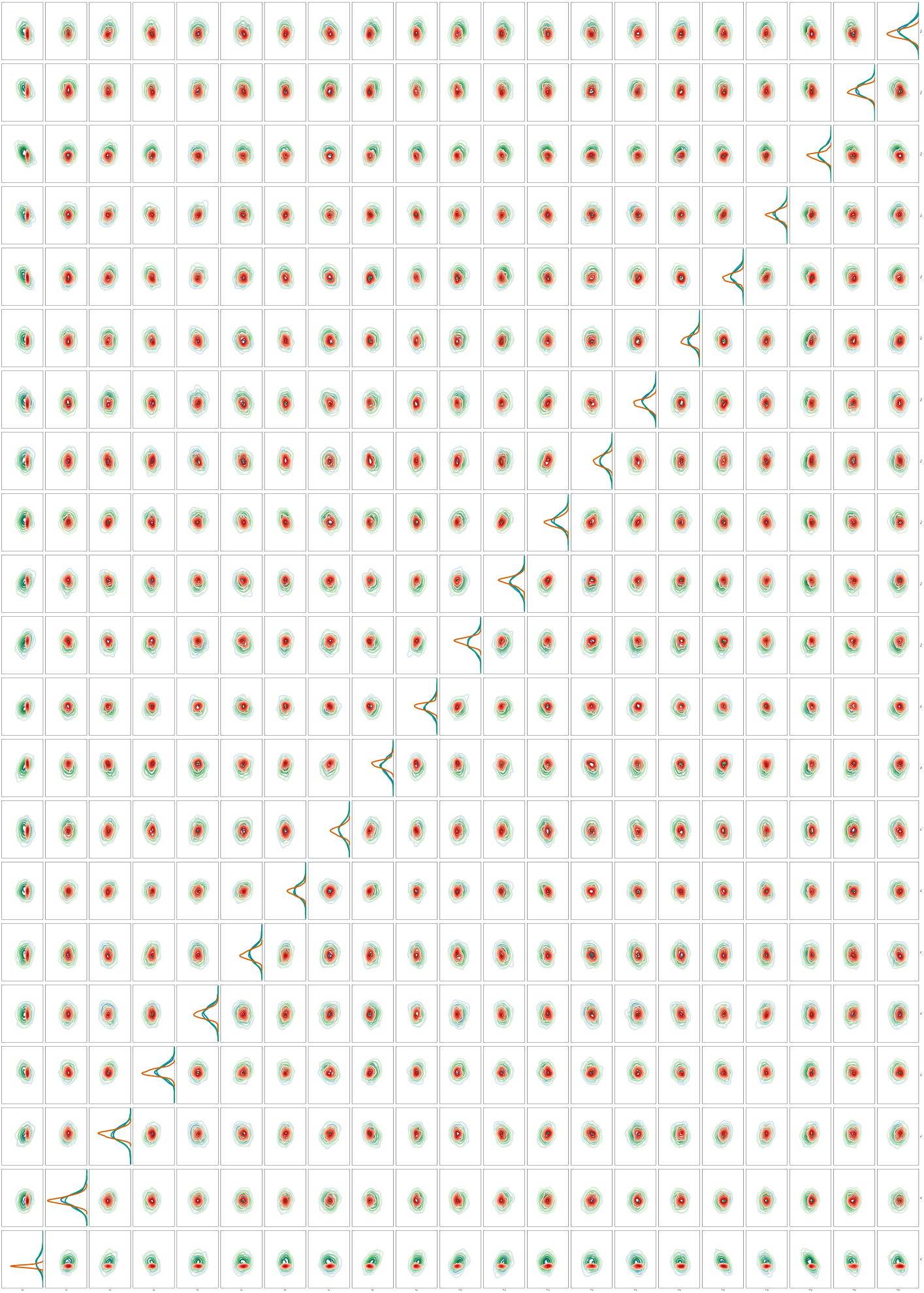
We fixed the prior $p(\bm{z})$ to be a zero-mean Gaussian given by: $p(\bm{z})=\mathcal{N}(\bm{0},100\times\bm{I}_{D\times D})$ . For the semi-implicit setting, $\bm{\epsilon}$ followed a standard Gaussian whose dimension varied across data-sets. $q_{\bm{\theta}}(\bm{z}|\bm{\epsilon})$ was again a Gaussian with parameterised mean (two layer neural network with 200 units each) but with a full covariance matrix: $q_{\bm{\theta}}(\bm{z}|\bm{\epsilon})=\mathcal{N}(\bm{\mu}_{\bm{\theta}_{1}}(\bm{\epsilon}),\bm{L}_{\bm{\theta}_{2}}\bm{L}_{\bm{\theta}_{2}}^{\mathsf{T}})$ . Due to space constraints, the full set of results can be found in the appendix. In the first two rows in Figures 1, we demonstrate violin plots on all three data-sets. Clearly CI-VI captures the variance better than Mean-Field Variational Bias (MFVB in the figure) when compared to MCMC distributions ¹³¹³ 13 Please note we also show a marginalised pair-wise posterior plot in the appendix. across all latent variables.

Semi-implicit Variational Autoencoders: In our final evaluation, we extensively experimented with variational autoencoders [19] but ones that exhibited semi-implicit variational distributions. In fact, it has been shown that upon the usage of semi-implicit variational distributions, the gap between the ELBO and marginal data likelihood can further be reduced [36, 46]. We experimented with three data-sets, two of which are standard (MNIST and Fashion-MNIST), while the third considered a text modelling task with the Penn-Tree-Bank (PTB) as presented in [8]. All structural details in each of these scenarios can be found in the appendix. Our results depicted in Figures 2 (bottom-row) compare CI-VI with semi-implicit solvers [36, 46], nested Monte-Carlo algorithms, and compositional optimisers. Again, it is clear that CI-VI outperforms others in terms of the number of epochs needed for convergence. Interestingly, such a gap is further signified on the PBT data-set¹⁴¹⁴ 14 Please note that we do not show the results of SIVI and UIVI in Figure 1 (h) as it was hard to get these to correctly operate on NLP tasks due to their source implementations. Staying fair to these methods, we opted-out of demonstrating their performance..

4 Conclusions and Future Work

We proposed CI-VI, a compositional solver for scalable and efficient semi-implicit variational inference. Our method rewrites SIVI as an instance of a compositional optimisation and devises a solver that correctly handles nested bias through an extrapolation-smoothing and a gradient sketching mechanism. We tested our method on a variety of tasks, including text modelling from natural language processing. In all these instances, we showed CI-VI’s effectiveness. In papers to follow, we plan to further scale our method to dialogue problems from NLP and to extend our analysis to time-series models. We also think our nested-expectation theoretical results can be broadly applied beyond this paper to cover topics from experimental design. We will also tackle this direction in the future.

References

[1] Zeyuan Allen Zhu and Elad Hazan. Variance Reduction for Faster Non-Convex Optimization. In Proceedings of the 33nd International Conference on Machine Learning, ICML 2016, volume 48, pages 699–707, 2016.
[2] Michael Betancourt. A Conceptual Introduction to Hamiltonian Monte Carlo. arXiv preprint arXiv:1701.02434, 2017.
[3] David M. Blei, Alp Kucukelbir, and Jon D. McAuliffe. Variational Inference: A Review for Statisticians. Journal of the American Statistical Association, 112(518):859–877, 2017.
[4] P.J. Davis and P. Rabinowitz. Methods of Numerical Integration. Dover Books on Mathematics Series. Dover Publications, 2007.
[5] Petros Drineas, Ravi Kannan, and Michael W. Mahoney. Fast Monte Carlo Algorithms for Matrices I: Approximating Matrix Multiplication. SIAM J. Comput., 36(1):132–157, July 2006.
[6] John Duchi, Elad Hazan, and Yoram Singer. Adaptive Subgradient Methods for Online Learning and Stochastic Optimization. J. Mach. Learn. Res., page 2121–2159, 2011.
[7] Cong Fang, Chris Junchi Li, Zhouchen Lin, and Tong Zhang. SPIDER: Near-Optimal Non-Convex Optimization via Stochastic Path-Integrated Differential Estimator. In Advances in Neural Information Processing Systems 31, NeurIPS 2018, pages 687–697, 2018.
[8] Hao Fu, Chunyuan Li, Ke Bai, Jianfeng Gao, and Lawrence Carin. Flexible Text Modeling with Semi-Implicit Latent Representations.
[9] Victor Gabillon, Rasul Tutunov, Michal Valko, and Haitham Bou Ammar. Derivative-Free & Order-Robust Optimisation. arXiv preprint arXiv:1910.04034, 2019.
[10] Ryan Giordano, Tamara Broderick, and Michael I. Jordan. Linear Response Methods for Accurate Covariance Estimates from Mean Field Variational Bayes. In Advances in Neural Information Processing Systems 28, NeurIPS 2015, pages 1441–1449, 2015.
[11] Karol Gregor, Ivo Danihelka, Alex Graves, Danilo Rezende, and Daan Wierstra. DRAW: A Recurrent Neural Network For Image Generation. In Proceedings of the 32nd International Conference on Machine Learning, ICML 2015, volume 37, pages 1462–1471, 2015.
[12] Shaobo Han, Xuejun Liao, David B. Dunson, and Lawrence Carin. Variational Gaussian Copula Inference. In Proceedings of the 19th International Conference on Artificial Intelligence and Statistics, AISTATS 2016, volume 51, pages 829–838, 2016.
[13] Matthew D. Hoffman, David M. Blei, Chong Wang, and John Paisley. Stochastic Variational Inference. J. Mach. Learn. Res., 14(1):1303–1347, 2013.
[14] Ferenc Huszár. Variational Inference using Implicit Distributions. CoRR, abs/1702.08235, 2017.
[15] Tommi S. Jaakkola and Michael I. Jordan. Variational Probabilistic Inference and the QMR-DT Network. J. Artif. Intell. Res., 10:291–322, 1999.
[16] Chi Jin, Rong Ge, Praneeth Netrapalli, Sham M. Kakade, and Michael I. Jordan. How to Escape Saddle Points Efficiently. In Proceedings of the 34th International Conference on Machine Learning, ICML 2017, volume 70, pages 1724–1732, 2017.
[17] D. C. Joyce. Survey of Extrapolation Process in Numerical Analysis. SIAM Review, 13(4):435–490, 1971.
[18] Diederik P. Kingma and Jimmy Ba. ADAM: A Method for Stochastic Optimization. In 3rd International Conference on Learning Representations, ICLR 2015, 2015.
[19] Diederik P. Kingma and Max Welling. Auto-Encoding Variational Bayes. In 2nd International Conference on Learning Representations, ICLR 2014, 2014.
[20] Huan Li and Zhouchen Lin. Accelerated Proximal Gradient Methods for Nonconvex Programming. In Advances in Neural Information Processing Systems 28, NeurIPS 2015, pages 379–387, 2015.
[21] Minne Li, Lisheng Wu, Jun Wang, and Haitham Bou-Ammar. Multi-View Reinforcement Learning. In Advances in Neural Information Processing Systems 32, NeurIPS 2019, pages 1418–1429, 2019.
[22] Yingzhen Li and Richard E. Turner. Gradient Estimators for Implicit Models. In 6th International Conference on Learning Representations, ICLR 2018, 2018.
[23] Liu Liu, Ji Liu, Cho-Jui Hsieh, and Dacheng Tao. Stochastically controlled stochastic gradient for the convex and non-convex composition problem, 2018.
[24] Lars Maaløe, Casper Kaae Sønderby, Søren Kaae Sønderby, and Ole Winther. Auxiliary Deep Generative Models. In Proceedings of The 33rd International Conference on Machine Learning, ICML 2016, volume 48, pages 1445–1453, 2016.
[25] Shakir Mohamed and Balaji Lakshminarayanan. Learning in Implicit Generative Models. CoRR, abs/1610.03483, 2016.
[26] Mahesh Chandra Mukkamala and Matthias Hein. Variants of RMSProp and Adagrad with Logarithmic Regret Bounds. In Proceedings of the 34th International Conference on Machine Learning, ICML 2017, page 2545–2553, 2017.
[27] Yuji Nakatsukasa. Approximate and Integrate: Variance Reduction in Monte Carlo Integration via Function Approximation. arXiv preprint arXiv:1806.05492, 2018.
[28] Yurii Nesterov. Introductory Lectures on Convex Optimization: A Basic Course. Springer Publishing Company, Incorporated, first edition, 2014.
[29] Adam Paszke, Sam Gross, Francisco Massa, Adam Lerer, James Bradbury, Gregory Chanan, Trevor Killeen, Zeming Lin, Natalia Gimelshein, Luca Antiga, Alban Desmaison, Andreas Kopf, Edward Yang, Zachary DeVito, Martin Raison, Alykhan Tejani, Sasank Chilamkurthy, Benoit Steiner, Lu Fang, Junjie Bai, and Soumith Chintala. PyTorch: An Imperative Style, High-Performance Deep Learning Library. In Advances in Neural Information Processing Systems 32, NeurIPS 2019, pages 8024–8035. 2019.
[30] Tom Rainforth, Robert Cornish, Hongseok Yang, and Andrew Warrington. On Nesting Monte Carlo Estimators. In Proceedings of the 35th International Conference on Machine Learning, ICML 2018, volume 80, pages 4264–4273, 2018.
[31] Rajesh Ranganath, Dustin Tran, and David M. Blei. Hierarchical Variational Models. 33rd International Conference on Machine Learning, ICML 2016, 1:515–528, 2016.
[32] Sashank J. Reddi, Satyen Kale, and Sanjiv Kumar. On the Convergence of ADAM and Beyond. In 6th International Conference on Learning Representations, ICLR 2018, 2018.
[33] Danilo Jimenez Rezende and Shakir Mohamed. Variational Inference with Normalizing Flows. In 32nd International Conference on Machine Learning, ICML 2015, volume 2, pages 1530–1538, 2015.
[34] Lawrence K. Saul and Michael Jordan. Exploiting Tractable Substructures in Intractable Networks. In Advances in Neural Information Processing Systems 8, NeurIPS 1996, pages 486–492, 1996.
[35] Jiaxin Shi, Shengyang Sun, and Jun Zhu. Kernel Implicit Variational Inference. 6th International Conference on Learning Representations, ICLR 2018, 2018.
[36] Michalis K. Titsias and Francisco J. R. Ruiz. Unbiased Implicit Variational Inference. In The 22nd International Conference on Artificial Intelligence and Statistics, AISTATS 2019, volume 89, pages 167–176, 2019.
[37] Dustin Tran, Rajesh Ranganath, and David M. Blei. The Variational Gaussian Process. In 4th International Conference on Learning Representations, ICLR 2016, pages 1–14, 2016.
[38] Dustin Tran, Rajesh Ranganath, and David M. Blei. Hierarchical Implicit Models and Likelihood-Free Variational Inference. In Advances in Neural Information Processing Systems 30, NeurIPS 2017, pages 5523–5533, 2017.
[39] Rasul Tutunov, Haitham Bou-Ammar, and Ali Jadbabaie. Distributed Newton Method for Large-Scale Consensus Optimization. IEEE Trans. Autom. Control., 64(10):3983–3994, 2019.
[40] Rasul Tutunov, Dongho Kim, and Haitham Bou Ammar. Distributed Multitask Reinforcement Learning with Quadratic Convergence. In Advances in Neural Information Processing Systems 31, NeurIPS 2018, pages 8907–8916. 2018.
[41] Rasul Tutunov, Minne Li, Jun Wang, and Haitham Bou-Ammar. Compositional ADAM: An Adaptive Compositional Solver. CoRR, abs/2002.03755, 2020.
[42] Don van Ravenzwaaij, Peter Cassey, and Scott Brown. A Simple Introduction to Markov Chain Monte–Carlo Sampling. Psychonomic Bulletin & Review, 25, 03 2016.
[43] Mengdi Wang, Ethan X. Fang, and Han Liu. Stochastic Compositional Gradient Descent: Algorithms for Minimizing Compositions of Expected-value Functions. Math. Program., 161(1-2):419–449, 2017.
[44] Mengdi Wang, Ji Liu, and Ethan Fang. Accelerating Stochastic Composition Optimization. In Advances in Neural Information Processing Systems 29, NeurIPS 2016, pages 1714–1722. 2016.
[45] Norbert Wiener. Extrapolation, Interpolation, and Smoothing of Stationary Time Series. The MIT Press, 1964.
[46] Mingzhang Yin and Mingyuan Zhou. Semi-Implicit Variational Inference. In Proceedings of the 35th International Conference on Machine Learning, ICML 2018, volume 80, pages 5646–5655, 2018.
[47] Manzil Zaheer, Sashank Reddi, Devendra Sachan, Satyen Kale, and Sanjiv Kumar. Adaptive Methods for Nonconvex Optimization. In Advances in Neural Information Processing Systems 31, NeurIPS 2018, pages 9793–9803. 2018.
[48] Matthew D. Zeiler. Adadelta: An Adaptive Learning Rate Method. CoRR, abs/1212.5701, 2012.
[49] Cheng Zhang, Judith Bütepage, Hedvig Kjellström, and Stephan Mandt. Advances in Variational Inference. IEEE Trans. Pattern Anal. Mach. Intell., 41(8):2008–2026, 2019.

Appendix A Practical implementation

To improve numerical stability and computational efficiency, our implementation of CI-VI has been adapted to properties of functions $f_{\nu}(\cdot)$ and $g_{\bm{\hat{\epsilon}}}(\cdot)$ defined in Section 2.2. These adaptions are clarified below:

Log trick:

The output from $g_{\bm{\hat{\epsilon}}}(\cdot)$ is a vector of density ratios whose value can be extreme, especially when the $\bm{z}$ and $\bm{x}$ are high-dimensional rvs. In order to do inference in such probabilistic model, we propose a CI-VI implementation which conducts most of the computations in log-scale. The sub-sampled gradient $\overline{\nabla\mathcal{L}(\bm{\theta}_{t})}$ in Algorithm 1 can be reformulated as:

	$\displaystyle\overline{\nabla\mathcal{L}(\bm{\theta}_{t})}=\overline{\nabla\bm{g}_{t}(\bm{\theta}_{t})}^{\mathsf{T}}\overline{\nabla f_{t}(\bm{y}_{t})}$	$\displaystyle=[\nabla\log\overline{\bm{g}_{t}(\bm{\theta}_{t})}^{\mathsf{T}}]_{p\times n}\cdot\underbrace{\exp\left[\log\overline{\bm{g}_{t}(\bm{\theta}_{t})}+\log\overline{\nabla f_{t}(\bm{y}_{t})}\right]_{n\times 1}}_{\bm{k}_{t}}$
	$\displaystyle\text{where}\quad\overline{f_{t}(\bm{y}_{t})}$	$\displaystyle=\nicefrac{{1}}{{K_{t}^{(1)}}}\sum_{i=1}^{K_{t}^{(1)}}[\log\bm{y}_{t}]^{\mathsf{T}}\bm{e}_{\nu_{t_{i}}}$

The $j$ -th element of $\bm{k}_{t}$ is then given by Equation 6. Since $\bm{y}_{t}$ is a smoothed average of $\overline{\bm{g}_{t}(\bm{\theta}_{t})}$ , their logarithms will cancel each other before the exponentiation is taken.

\displaystyle(\bm{k}_{t})_{j}=\begin{cases}0,\quad\textit{if}\ \ \sum_{i=1}^{K_{t}^{(1)}}\mathcal{I}(\nu_{t_{i}}=j)=0\\ \exp(\log\overline{\bm{g}_{t}(\bm{\theta}_{t})}_{j}-\log{K_{t}^{(1)}}-{\log(\bm{y}_{t}})_{j}+\log\sum_{i=1}^{K_{t}^{(1)}}\mathbb{I}(\nu_{t_{i}}=j)),\quad\textit{otherwise}\\ \end{cases}

(6)

Finalising this log-scale implementation, we track the value of $\log\bm{y}_{t}$ instead of $\bm{y}_{t}$ for the auxiliary update as follow:

\displaystyle\bm{a}\coloneqq\log(1-\beta_{t})+\log\bm{y}_{t},\quad\bm{b}\coloneqq\log\beta_{t}+\log\overline{\bm{g}_{t}(\bm{z}_{t+1})},\quad\log\bm{y}_{t+1}=\log[\exp(\bm{a})+\exp(\bm{b})]

The update of $\log\bm{y}_{t}$ may encounter numerical overflow, which can be handled by Taylor series approximation. For the $j$ -th overflowed dimension, $\bm{r}_{j}\coloneqq\exp[\max(\bm{a}_{j},\bm{b}_{j})-\min(\bm{a}_{j},\bm{b}_{j})],\ \ \log(\bm{y}_{t+1})_{j}=\max(\bm{a}_{j},\bm{b}_{j})+\sum_{i=1}^{N}\frac{(-1)^{i-1}\bm{r}_{j}^{i}}{i}+\mathcal{O}(\bm{r}_{j}^{N+1})$ .

For large-scale CI-VI, updating all dimensions of $\log\bm{y}_{t}$ is challenging due to computational and memory constraints. Rather than performing a full update for $\log\bm{y}_{t}$ , we follow a batch-like mechanism that proved effective in our experiments. Namely, we split the index set $[1,n]$ into smaller chunks and sample $\nu_{t}$ from one of these chunks to execute the updates. This way, only those dimensions indexed by the current chunk need to be updated rather than the whole high-dimensional vector $\log\bm{y}_{t}$ . Of course, such chunks have to vary across iterations so as to guarantee the update of $\log\bm{y}_{t}$ . To do so, we switch to a new chunk occasionally and re-initialize the dimensions of $\log\bm{y}_{t}$ indexed by the new chunk using the value of $\log\overline{\bm{g}_{t}(\bm{z}_{t})}$ .

Sparse gradient-sketching:

Another insight from Equation 6 is that the $\bm{k}_{t}$ is a sparse vector with non-zero elements indexed by sampled $\nu_{t}$ . The gradient-sketching in Algorithm 2 can be adapted by removing the zero elements in $\bm{k}_{t}$ and corresponding columns in $[\nabla\log\overline{\bm{g}_{t}(\bm{\theta}_{t})}^{\mathsf{T}}]_{p\times n}$ first. The set $S_{t}$ is then sampled uniformly from the left indices.

Appendix B Experimental settings and results

Toy Experiments:

In toy experiments, we minimize the KL-divergence between semi-implict variational distributions $q_{\bm{\theta}}(\bm{z})$ and ground-truth distributions $p(\bm{z})$ . The compositional objective can be written as:

\displaystyle\mathcal{KL}[q_{\bm{\theta}}(\bm{z})||p(\bm{z})]=\mathbb{E}_{\bm{u}\sim q(\bm{u}),\bm{\epsilon}\sim q(\bm{\epsilon})}\left[\log\mathbb{E}_{\bm{\hat{\epsilon}}\sim q(\bm{\epsilon})}\left[\frac{q_{\bm{\theta}}(h_{\bm{\theta}}(\bm{u};\bm{\epsilon})|\bm{\hat{\epsilon}})}{p(h_{\bm{\theta}}(\bm{u};\bm{\epsilon}))}\right]\right].

Bayesian Logistic Regression:

Given a data-set $\mathcal{D}=\{\bm{x}_{i},y_{i}\}_{i=1}^{N}$ , we can write the compositional form of negative ELBO as:

	$\displaystyle-ELBO$	$\displaystyle=\mathbb{E}_{q_{\bm{\theta}}(\bm{z})}\left[\log\frac{q_{\bm{\theta}}(\bm{z})}{p(\mathcal{D}\|\bm{z})p(\bm{z})}\right]$
		$\displaystyle=\mathbb{E}_{\bm{u}\sim q(\bm{u}),\bm{\epsilon}\sim q(\bm{\epsilon})}\left[\log\mathbb{E}_{\bm{\hat{\epsilon}}\sim q(\bm{\epsilon})}\left[\frac{q_{\bm{\theta}}(h_{\bm{\theta}}(\bm{u};\bm{\epsilon})\|\bm{\hat{\epsilon}})}{p(\mathcal{D}\|h_{\bm{\theta}}(\bm{u};\bm{\epsilon}))\cdot p(h_{\bm{\theta}}(\bm{u};\bm{\epsilon}))}\right]\right],$

where $p(\mathcal{D}|\bm{z})=\prod_{i=1}^{N}p(y_{i}|\bm{x}_{i},\bm{z})=\prod_{i=1}^{N}\text{Bernoulli}\left[(1+\exp(-\bm{x}_{i}^{\mathsf{T}}\bm{z}))^{-1}\right]$ .

Semi-implicit Variational Autoencoder:

Given a dataset $\mathcal{D}=\{{\bm{x}_{i}}\}_{i=1}^{N}$ , the negative ELBO of a single datapoint $\bm{x}_{i}$ is given by:

\displaystyle-ELBO(\bm{x}_{i})=\mathbb{E}_{\bm{u}_{i}\sim q(\bm{u}),\bm{\epsilon}_{i}\sim q(\bm{\epsilon})}\left[\log\mathbb{E}_{\bm{\hat{\epsilon}}_{i}\sim p({\bm{\hat{\epsilon}}_{i}})}\left[\frac{q_{\bm{\theta}}(h_{\bm{\theta}}(\bm{u}_{i};\bm{\epsilon}_{i})|\bm{\hat{\epsilon}}_{i},\bm{x}_{i})}{p_{\bm{\hat{\theta}}}(\bm{x}_{i}|h_{\bm{\theta}}(\bm{u}_{i};\bm{\epsilon}_{i}))\cdot p(h_{\bm{\theta}}(\bm{u}_{i};\bm{\epsilon}_{i}))}\right]\right],

in which the encoder parameter $\bm{\theta}$ and decoder parameter $\bm{\hat{\theta}}$ are optimized jointly. We can further construct an estimator of the negative ELBO of the full data-set:

\displaystyle-ELBO(\mathcal{D})=N\cdot\mathbb{E}_{\bm{x}_{i}\sim\text{Uniform}(\mathcal{D}),\bm{u}_{i}\sim q(\bm{u}),\bm{\epsilon}_{i}\sim q(\bm{\epsilon})}\left[\log\mathbb{E}_{\bm{\hat{\epsilon}}_{i}\sim p({\bm{\hat{\epsilon}}_{i}})}\left[\frac{q_{\bm{\theta}}(h_{\bm{\theta}}(\bm{u}_{i};\bm{\epsilon}_{i})|\bm{\hat{\epsilon}}_{i},\bm{x}_{i})}{p_{\bm{\hat{\theta}}}(\bm{x}_{i}|h_{\bm{\theta}}(\bm{u}_{i};\bm{\epsilon}_{i}))\cdot p(h_{\bm{\theta}}(\bm{u}_{i};\bm{\epsilon}_{i}))}\right]\right],

All the experimental settings are listed below:

Two-Modal	Star	Banana
$\begin{aligned} &0.5\mathcal{N}\left(\begin{bmatrix}-2\\ 0\end{bmatrix},I_{2\times 2}\right)+\\ &0.5\mathcal{N}\left(\begin{bmatrix}2\\ 0\end{bmatrix},I_{2\times 2}\right)\end{aligned}$	$\begin{aligned} &0.5\mathcal{N}\left(0,\begin{bmatrix}2&1.8\\ 1.8&2\end{bmatrix}\right)+\\ &0.5\mathcal{N}\left(0,\begin{bmatrix}2&-1.8\\ -1.8&2\end{bmatrix}\right)\end{aligned}$	$\begin{aligned} &\bm{z}=\begin{bmatrix}\bm{z}_{1}\\ \bm{z}_{2}-\bm{z}_{1}^{2}-1\end{bmatrix}\\ \begin{bmatrix}\bm{z}_{1}\\ \bm{z}_{2}\end{bmatrix}&\sim\mathcal{N}\left(0,\begin{bmatrix}1&0.9\\ 0.9&1\end{bmatrix}\right)\end{aligned}$

Table 1: Ground-truth distributions used in toy experiments

	Two-Modal	Star	Banana
$q(\bm{\epsilon})$	$\mathcal{N}\left(\bm{0},I_{3\times 3}\right)$	$\mathcal{N}\left(\bm{0},I_{3\times 3}\right)$	$\mathcal{N}\left(\bm{0},I_{3\times 3}\right)$
$q_{\bm{\theta}}(\bm{z}\|\bm{\epsilon})$	$\mathcal{N}(\bm{\mu}_{\bm{\theta}_{1}}(\bm{\epsilon}),diag(\bm{\theta}_{2}))$	$\mathcal{N}(\bm{\mu}_{\bm{\theta}_{1}}(\bm{\epsilon}),diag(\bm{\theta}_{2}))$	$\mathcal{N}(\bm{\mu}_{\bm{\theta}_{1}}(\bm{\epsilon}),diag(\bm{\theta}_{2}))$
$\bm{\mu}_{\bm{\theta}_{1}}$	Hidden units: (50, 50) Hidden activation: ReLU Initializer: Xavier_normal	Hidden units: (50, 50) Hidden activation: ReLU Initializer: Xavier_normal	Hidden units: (50, 50) Hidden activation: ReLU Initializer: Xavier_normal
Hyper params	$K^{(1)}_{t}=1\cdot 10^{2}$ $K^{(2)}_{t}=1\cdot 10^{3}$ $C_{\alpha}=3\cdot 10^{-4}$ $C_{\beta}=0.99$ $C_{\gamma}=0.9$ $\mu=0.999$	$K^{(1)}_{t}=2\cdot 10^{2}$ $K^{(2)}_{t}=2\cdot 10^{3}$ $C_{\alpha}=2\cdot 10^{-4}$ $C_{\beta}=0.999$ $C_{\gamma}=0.9$ $\mu=0.999$	$K^{(1)}_{t}=2\cdot 10^{2}$ $K^{(2)}_{t}=2\cdot 10^{3}$ $C_{\alpha}=3\cdot 10^{-4}$ $C_{\beta}=0.999$ $C_{\gamma}=1.0$ $\mu=0.999$
Time elapsed	0.037 sec/iter $\times$ 200 iters 7.432 sec	0.040 sec/iter $\times$ 300 iters 11.972 sec	0.042 sec/iter $\times$ 300 iters 12.604 sec

Table 2: Experimental settings for toy examples

	Spam	Nodal	Waveform
$q(\bm{\epsilon})$	$\mathcal{N}\left(\bm{0},100\cdot I_{3\times 3}\right)$	$\mathcal{N}\left(\bm{0},100\cdot I_{3\times 3}\right)$	$\mathcal{N}\left(\bm{0},100\cdot I_{10\times 10}\right)$
$q_{\bm{\theta}}(\bm{z}\|\bm{\epsilon})$	$\mathcal{N}(\bm{\mu}_{\bm{\theta}_{1}}(\bm{\epsilon}),\bm{L}_{\bm{\theta}_{2}}\bm{L}_{\bm{\theta}_{2}}^{\mathsf{T}}),\penalty\ \bm{z}\in\mathbb{R}^{3}$	$\mathcal{N}(\bm{\mu}_{\bm{\theta}_{1}}(\bm{\epsilon}),\bm{L}_{\bm{\theta}_{2}}\bm{L}_{\bm{\theta}_{2}}^{\mathsf{T}}),\penalty\ \bm{z}\in\mathbb{R}^{6}$	$\mathcal{N}(\bm{\mu}_{\bm{\theta}_{1}}(\bm{\epsilon}),\bm{L}_{\bm{\theta}_{2}}\bm{L}_{\bm{\theta}_{2}}^{\mathsf{T}}),\penalty\ \bm{z}\in\mathbb{R}^{22}$
$\bm{\mu}_{\bm{\theta}_{1}}(\bm{\epsilon})$	Hidden units: (200, 200) Hidden activation: ReLU Initializer: Xavier_normal	Hidden units: (200, 200) Hidden activation: ReLU Initializer: Xavier_normal	Hidden units: (200, 200) Hidden activation: ReLU Initializer: Xavier_normal
Hyper params	$K^{(1)}_{t}=5\cdot 10^{1}$ $K^{(2)}_{t}=5\cdot 10^{2}$ $C_{\alpha}^{(\bm{\theta}_{1})}=1.5\cdot 10^{-4}$ $C_{\alpha}^{(\bm{\theta}_{2})}=2\cdot 10^{-1}$ $C_{\beta}=0.999$ $C_{\gamma}^{(\bm{\theta}_{1})}=0.7$ $C_{\gamma}^{(\bm{\theta}_{2})}=0.6$ $\mu=0.999$	$K^{(1)}_{t}=2\cdot 10^{2}$ $K^{(2)}_{t}=2\cdot 10^{3}$ $C_{\alpha}^{(\bm{\theta}_{1})}=1.7\cdot 10^{-4}$ $C_{\alpha}^{(\bm{\theta}_{2})}=1.7\cdot 10^{-4}$ $C_{\beta}=0.99$ $C_{\gamma}^{(\bm{\theta}_{1})}=0.75$ $C_{\gamma}^{(\bm{\theta}_{2})}=0.85$ $\mu=0.999$	$K^{(1)}_{t}=1\cdot 10^{2}$ $K^{(2)}_{t}=1\cdot 10^{3}$ $C_{\alpha}^{(\bm{\theta}_{1})}=3\cdot 10^{-4}$ $C_{\alpha}^{(\bm{\theta}_{2})}=2.5\cdot 10^{-4}$ $C_{\beta}=0.999$ $C_{\gamma}^{(\bm{\theta}_{1})}=0.85$ $C_{\gamma}^{(\bm{\theta}_{2})}=0.85$ $\mu=0.999$
Time elapsed	0.024 sec/iter $\times$ 600 iters 14.180 sec	0.015 sec/iter $\times$ 600 iters 8.986 sec	0.015 sec/iter $\times$ 3000 iters 45.761 sec

Table 3: Experimental settings for Bayesian logistic regression

Figure 3: Boxplot of marginal posteriors (left) and marginal & pairwise joint-posteriors (right) using MCMC, CIVI and MFVB on Spam data-set (top row) and Nodal data-set (bottom row). On the right (grid plots), MCMC is blue, CIVI is green and MFVB is orange.

Figure 4: Boxplot of marginal posteriors using MCMC, CIVI and MFVB on Waveform data-set.

	MNIST	FasionMNIST	PBT
$q(\bm{\epsilon})$	$\mathcal{N}\left(\bm{0},I_{10\times 10}\right)$	$\mathcal{N}\left(\bm{0},I_{10\times 10}\right)$	$\mathcal{N}\left(\bm{0},I_{10\times 10}\right)$
$q_{\bm{\theta}}(\bm{z}\|\bm{\epsilon},\bm{x}_{i})$	$\mathcal{N}(\bm{\mu}_{\bm{\theta}_{1}}(\bm{\epsilon},\bm{x}_{i}),diag(\bm{\theta}_{2}))$ $\bm{z}\in\mathbb{R}^{10}$	$\mathcal{N}(\bm{\mu}_{\bm{\theta}_{1}}(\bm{\epsilon},\bm{x}_{i}),diag(\bm{\theta}_{2}))$ $\bm{z}\in\mathbb{R}^{10}$	$\mathcal{N}(\bm{\mu}_{\bm{\theta}_{1}}(\bm{\epsilon},\bm{x}_{i}),diag(\bm{\theta}_{2}))$ $\bm{z}\in\mathbb{R}^{20}$
$\bm{\mu}_{\bm{\theta}_{1}}(\bm{\epsilon},\bm{x}_{i})$	Hidden units: (200, 200) Hidden activation: ReLU Initializer: Xavier_normal	Hidden units: (200, 200) Hidden activation: ReLU Initializer: Xavier_normal	Embedding dim: 256 LSTM hidden dim: 256 MLP hidden dim: 256 MLP activation: ReLU
$p_{\bm{\hat{\theta}}}(\bm{x}_{i}\|\bm{z})$	$\prod_{i=1}^{D}\text{Bernoulli}[\pi_{\bm{\hat{\theta}}}(\bm{z})]$	$\prod_{i=1}^{D}\text{Bernoulli}[\pi_{\bm{\hat{\theta}}}(\bm{z})]$	$\prod_{i=1}^{D}\text{Categorical}[\bm{\pi}_{\bm{\hat{\theta}}}(\bm{z})]$
$\bm{\pi}_{\bm{\hat{\theta}}}(\bm{z})$	Hidden units: (200, 200) Hidden activation: ReLU Initializer: Xavier_normal	Hidden units: (200, 200) Hidden activation: ReLU Initializer: Xavier_normal	Embedding dim: 256 LSTM hidden dim: 256
Hyper params	$K^{(1)}_{t}=300$ $K^{(2)}_{t}=30$ $C_{\alpha}^{(\bm{\theta}_{1})}=1\cdot 10^{-5}$ $C_{\alpha}^{(\bm{\theta}_{2})}=1\cdot 10^{-4}$ $C_{\alpha}^{(\bm{\hat{\theta}})}=5\cdot 10^{-4}$ $C_{\beta}=0.999$ $C_{\gamma}^{(\bm{\theta}_{1})}=0.2$ $C_{\gamma}^{(\bm{\theta}_{2})}=0.2$ $C_{\gamma}^{(\bm{\hat{\theta}})}=0.2$ $\mu=0.999$	$K^{(1)}_{t}=300$ $K^{(2)}_{t}=30$ $C_{\alpha}^{(\bm{\theta}_{1})}=1\cdot 10^{-5}$ $C_{\alpha}^{(\bm{\theta}_{2})}=1\cdot 10^{-4}$ $C_{\alpha}^{(\bm{\hat{\theta}})}=5\cdot 10^{-4}$ $C_{\beta}=0.999$ $C_{\gamma}^{(\bm{\theta}_{1})}=0.2$ $C_{\gamma}^{(\bm{\theta}_{2})}=0.2$ $C_{\gamma}^{(\bm{\hat{\theta}})}=0.2$ $\mu=0.999$	$K^{(1)}_{t}=320$ $K^{(2)}_{t}=100$ $C_{\alpha}^{(\bm{\theta}_{1})}=2\cdot 10^{-4}$ $C_{\alpha}^{(\bm{\theta}_{2})}=2\cdot 10^{-4}$ $C_{\alpha}^{(\bm{\hat{\theta}})}=5\cdot 10^{-4}$ $C_{\beta}=0.99$ $C_{\gamma}^{(\bm{\theta}_{1})}=0.1$ $C_{\gamma}^{(\bm{\theta}_{2})}=0.1$ $C_{\gamma}^{(\bm{\hat{\theta}})}=0.1$ $\mu=0.999$
Time elapsed	0.0218 sec/iter $\times$ 18000 iters 392 sec	0.0236 sec/iter $\times$ 18000 iters 425 sec	0.0989 sec/iter $\times$ 40000 iters 3956 sec

Table 4: Experimental settings for variational autoencoder.

Method	Time (ms) per iteration
SIVI	155
UIVI	69
ASCPG	157
SCGD	152
CI-VI [this paper]	56

Table 5: Average time per iteration for training VAE on Intel i9-9900X 3.50GHz CPU

Appendix C Detailed Descriptions of Assumptions

Due to the lack of space, we provide more detailed description of all assumptions required to establish theoretical convergence results for the proposed CI-VI Algorithm in this section.

Recall, we target the following nested optimisation problem:

\min_{\boldsymbol{\theta}\in\mathbb{R}^{p}}\mathcal{L}(\boldsymbol{\theta})=\mathbb{E}_{\nu}\left[f_{\nu}\left(\mathbb{E}_{\boldsymbol{\hat{\epsilon}}}\left[\boldsymbol{g}_{\boldsymbol{\hat{\epsilon}}}(\boldsymbol{\theta})\right]\right)\right]

(7)

where for any $\nu,\boldsymbol{\hat{\epsilon}}$ we have $f_{\nu}(\cdot):\mathbb{R}^{n}\to\mathbb{R}$ and $\boldsymbol{g}_{\boldsymbol{\hat{\epsilon}}}(\cdot):\mathbb{R}^{p}\to\mathbb{R}^{n}$ and random variables $\nu,\boldsymbol{\hat{\epsilon}}$ follow some unknown distributions $\nu\sim\text{p}_{\nu}(\cdot)$ and $\boldsymbol{\hat{\epsilon}}\sim\text{p}_{\boldsymbol{\hat{\epsilon}}}(\cdot)$ correspondingly. Please notice, we do not assume that these distributions are independent. For brevity, let us denote $f(\boldsymbol{y})=\mathbb{E}_{\nu}[f_{\nu}(\boldsymbol{y})]$ and $\boldsymbol{g}(\boldsymbol{\theta})=\mathbb{E}_{\boldsymbol{\hat{\epsilon}}}[\boldsymbol{g}_{\boldsymbol{\hat{\epsilon}}}(\boldsymbol{\theta})]$ , then it is easy to see:

		$\displaystyle\mathcal{L}(\boldsymbol{\theta})=f(\boldsymbol{g}(\boldsymbol{\theta})),$
		$\displaystyle\nabla\mathcal{L}(\boldsymbol{\theta})=\mathbb{E}_{\boldsymbol{\hat{\epsilon}}}[\nabla\boldsymbol{g}_{\boldsymbol{\hat{\epsilon}}}(\boldsymbol{\theta})^{\mathsf{T}}]\mathbb{E}_{\nu}[\nabla f_{\nu}(\mathbb{E}_{\boldsymbol{\hat{\epsilon}}}[\boldsymbol{g}_{\boldsymbol{\hat{\epsilon}}}(\boldsymbol{\theta})])]=\nabla\boldsymbol{g}(\boldsymbol{\theta})^{\mathsf{T}}\nabla f(\boldsymbol{g}(\boldsymbol{\theta})).$

Let the following assumption holds:

Assumption 1:

1.

Function $f_{\nu}(\cdot)$ is bounded, i.e. $\forall\boldsymbol{y}\in\mathbb{R}^{n}$ :

$|f_{\nu}(\boldsymbol{y})|\leq B_{f}.$

for any $v$ .

Function $f_{\nu}(\cdot)$ is $L_{f}-$ smooth. i.e. $\forall\boldsymbol{y}_{1},\boldsymbol{y}_{2}\in\mathbb{R}^{n}$ :

||\nabla f_{\nu}(\boldsymbol{y}_{1})-\nabla f_{\nu}(\boldsymbol{y}_{2})||_{2}\leq L_{f}||\boldsymbol{y}_{1}-\boldsymbol{y}_{2}||_{2}.

for any $v$ .

3.

Function $f_{\nu}(\cdot)$ has bounded gradient, i.e $\forall\boldsymbol{y}\in\mathbb{R}^{n}$ :

$\displaystyle||\nabla f_{\nu}(\boldsymbol{y})||_{2}\leq M_{f}.$

for any $v$ .

Mapping $\boldsymbol{g}_{\boldsymbol{\hat{\epsilon}}}(\boldsymbol{\theta})$ is $M_{g}$ Lipschitz continuous, i.e. $\forall\boldsymbol{\theta},\boldsymbol{z}\in\mathbb{R}^{p}$ :

||\boldsymbol{g}_{\boldsymbol{\hat{\epsilon}}}(\boldsymbol{\theta})-\boldsymbol{g}_{\boldsymbol{\hat{\epsilon}}}(\boldsymbol{z})||_{2}\leq M_{g}||\boldsymbol{\theta}-\boldsymbol{z}||_{2}.

for any ${\boldsymbol{\hat{\epsilon}}}$ .

Mapping $\boldsymbol{g}_{\boldsymbol{\hat{\epsilon}}}(\boldsymbol{\theta})$ is $L_{g}-$ smooth. i.e. $\forall\boldsymbol{\theta,z}\in\mathbb{R}^{p}$ :

||\nabla\boldsymbol{g}_{\boldsymbol{\hat{\epsilon}}}(\boldsymbol{\theta})-\nabla\boldsymbol{g}_{\boldsymbol{\hat{\epsilon}}}(\boldsymbol{z})||_{2}\leq L_{g}||\boldsymbol{\theta}-\boldsymbol{z}||_{2}.

for any ${\boldsymbol{\hat{\epsilon}}}$ .

Because distributions $\nu\sim\text{p}_{\nu}(\cdot)$ and $\boldsymbol{\hat{\epsilon}}\sim\text{p}_{\boldsymbol{\hat{\epsilon}}}(\cdot)$ are unknown, we assume the presence of two first order oracles $\mathcal{FOO}_{f}$ and $\mathcal{FOO}_{g}$ , such that given fixed vectors $\boldsymbol{z}_{t}\in\mathbb{R}^{p}$ , $\boldsymbol{y}_{t}\in\mathbb{R}^{n}$ and integer numbers $K^{(1)}_{t}$ and $K^{(2)}_{t}$ at time step $t$ they return the following collections:

		$\displaystyle\mathcal{FOO}_{f}[\boldsymbol{y}_{t},K^{(1)}_{t}]=\{\nu_{t_{a}},\nabla f_{\nu_{t_{a}}}(\boldsymbol{y}_{t})\}^{K^{(1)}_{t}}_{a=1},\ \ \ \ \ \text{where }\ \{\nu_{t_{a}}\}^{K^{(1)}_{t}}_{a=1}\ \ \ \text{are i.i.d}$		(8)
		$\displaystyle\mathcal{FOO}_{g}[\boldsymbol{z}_{t},K^{(2)}_{t}]=\{{\boldsymbol{\hat{\epsilon}}_{t_{a}}},\boldsymbol{g}_{{\boldsymbol{\hat{\epsilon}}_{t_{a}}}}(\boldsymbol{z}_{t}),\nabla\boldsymbol{g}_{{\boldsymbol{\hat{\epsilon}}_{t_{a}}}}(\boldsymbol{z}_{t})\}^{K^{(2)}_{t}}_{a=1},\ \ \ \ \ \text{where }\ \{{\boldsymbol{\hat{\epsilon}}_{t_{a}}}\}^{K^{(2)}_{t}}_{a=1}\ \ \ \text{are i.i.d}$

The complexity of the proposed algorithm will be evaluated in terms of total number of calls to first order oracles $\mathcal{FOO}_{f}[\cdot,\cdot]$ , $\mathcal{FOO}_{g}[\cdot,\cdot]$ .

Assumption 2: At any given time step $t$ , the oracles $\mathcal{FOO}_{f}[\boldsymbol{y}]_{t}$ and $\mathcal{FOO}_{g}[\boldsymbol{z}]_{t}$ satisfy the following two conditions for any $\boldsymbol{z}\in\mathbb{R}^{p}$ and $\boldsymbol{y}\in\mathbb{R}^{n}$ :

Sample collections

\displaystyle\left(\{\nu_{1_{a}}\}^{K^{(1)}_{1}}_{a=1},\{\boldsymbol{\hat{\epsilon}}_{1_{a}}\}^{K^{(2)}_{1}}_{a=1}\right),\left(\{\nu_{2_{a}}\}^{K^{(1)}_{2}}_{a=1},\{\boldsymbol{\hat{\epsilon}}_{2_{a}}\}^{K^{(2)}_{2}}_{a=1}\right),\ldots,\left(\{\nu_{t_{a}}\}^{K^{(1)}_{t}}_{a=1},\{{\boldsymbol{\hat{\epsilon}}_{t_{a}}}\}^{K^{(2)}_{t}}_{a=1}\right)

are independent.

Unbiased estimates: for any $\boldsymbol{\theta}\in\mathbb{R}^{p}$ , $\boldsymbol{y}\in\mathbb{R}^{n}$ :

		$\displaystyle\mathbb{E}_{{\boldsymbol{\hat{\epsilon}}_{t_{a}}}}\left[\boldsymbol{g}_{{\boldsymbol{\hat{\epsilon}}_{t_{a}}}}(\boldsymbol{\theta})\right]=\mathbb{E}_{\boldsymbol{\hat{\epsilon}}}\left[\boldsymbol{g}_{\boldsymbol{\hat{\epsilon}}}(\boldsymbol{\theta})\right],$
		$\displaystyle\mathbb{E}_{{\boldsymbol{\hat{\epsilon}}_{t_{a}}},\nu_{t_{b}}}\left[\nabla\boldsymbol{g}^{\mathsf{T}}_{{\boldsymbol{\hat{\epsilon}}_{t_{a}}}}(\boldsymbol{\theta})\nabla f_{\nu_{t_{b}}}(\boldsymbol{y})\right]=\mathbb{E}_{\boldsymbol{\hat{\epsilon}}}\left[\nabla\boldsymbol{g}^{\mathsf{T}}_{\boldsymbol{\hat{\epsilon}}}(\boldsymbol{\theta})\right]\mathbb{E}_{\nu}\left[\nabla f_{\nu}(\boldsymbol{y})\right].$

for any $t$ and $a\in[1,\ldots,K^{(2)}_{t}]$ , $b\in[1,\ldots,K^{(1)}_{t}]$ .

Bounded variance of stochastic gradients: for any $\boldsymbol{\theta}\in\mathbb{R}^{p}$ , $\boldsymbol{y}\in\mathbb{R}^{n}$ :

		$\displaystyle\mathbb{E}_{\nu_{t_{b}}}\|\|\nabla f_{\nu_{t_{b}}}(\boldsymbol{y})-\nabla\mathbb{E}_{\nu}\left[f_{\nu}(\boldsymbol{y})\right]\|\|^{2}_{2}\leq\sigma^{2}_{1},$
		$\displaystyle\mathbb{E}_{{\boldsymbol{\hat{\epsilon}}_{t_{a}}}}\|\|\nabla\boldsymbol{g}_{{\boldsymbol{\hat{\epsilon}}_{t_{a}}}}(\boldsymbol{\theta})-\nabla\mathbb{E}_{\boldsymbol{\hat{\epsilon}}}\left[\boldsymbol{g}_{\boldsymbol{\hat{\epsilon}}}(\boldsymbol{\theta})\right]\|\|^{2}_{2}\leq\sigma^{2}_{2},$
		$\displaystyle\mathbb{E}_{{\boldsymbol{\hat{\epsilon}}_{t_{a}}}}\left[\|\|\boldsymbol{g}_{{\boldsymbol{\hat{\epsilon}}_{t_{a}}}}(\boldsymbol{\theta})-\boldsymbol{g}(\boldsymbol{\theta})\|\|^{2}_{2}\right]\leq\sigma^{2}_{3}.$

for any $t$ and $a\in[1,\ldots,K^{(2)}_{t}]$ , $b\in[1,\ldots,K^{(1)}_{t}]$ .

Appendix D Theoretical Guarantees

In this section, we establish all theoretical results needed for proving the main theorem and then present its proof.

D.1 L-smoothness of function $\mathcal{L}(\cdot)$

Our first result provides the important property of the overall compositional function $\mathcal{L}(\cdot)$ which will be used later in the convergence analysis of the proposed CI-VI Algorithm.

Lemma: Let Assumptions 1 and 2 hold, then function $\mathcal{L}(\cdot)$ is $L-$ Lipschitz smooth, i,e:

||\nabla\mathcal{L}(\boldsymbol{\theta}_{1})-\nabla\mathcal{L}(\boldsymbol{\theta}_{2})||_{2}\leq L||\boldsymbol{\theta}_{1}-\boldsymbol{\theta}_{2}||_{2}\ \ \ \ \ \ \ \ \ \forall\boldsymbol{\theta}_{1},\boldsymbol{\theta}_{2}\in\mathbb{R}^{p}

(9)

with $L=M^{2}_{g}L_{f}+L_{g}M_{f}$ .

Proof.

Assumption 1 implies that $||\nabla\boldsymbol{g}_{\boldsymbol{\hat{\epsilon}}}(\boldsymbol{\theta})||_{2}\leq M_{g}$ for any $\boldsymbol{\theta}\in\mathbb{R}^{p}$ . Hence, using Jensen inequality as well as property of the norm we have:

		$\displaystyle\|\|\nabla\mathcal{L}(\boldsymbol{\theta}_{1})-\nabla\mathcal{L}(\boldsymbol{\theta}_{2})\|\|_{2}=$
		$\displaystyle\|\|\mathbb{E}_{\boldsymbol{\hat{\epsilon}}}\left[\nabla\boldsymbol{g}^{\mathsf{T}}_{\boldsymbol{\hat{\epsilon}}}(\boldsymbol{\theta}_{1})\right]\mathbb{E}_{\nu}\left[\nabla f_{\nu}\left(\mathbb{E}_{\boldsymbol{\hat{\epsilon}}}\left[\boldsymbol{g}_{\boldsymbol{\hat{\epsilon}}}(\boldsymbol{\theta}_{1})\right]\right)\right]-\mathbb{E}_{\boldsymbol{\hat{\epsilon}}}\left[\nabla\boldsymbol{g}^{\mathsf{T}}_{\boldsymbol{\hat{\epsilon}}}(\boldsymbol{x_{2}})\right]\mathbb{E}_{\nu}\left[\nabla f_{\nu}\left(\mathbb{E}_{\boldsymbol{\hat{\epsilon}}}\left[\boldsymbol{g}_{\boldsymbol{\hat{\epsilon}}}(\boldsymbol{\theta}_{2})\right]\right)\right]\|\|_{2}\leq$
		$\displaystyle\|\|\mathbb{E}_{\boldsymbol{\hat{\epsilon}}}\left[\nabla\boldsymbol{g}^{\mathsf{T}}_{\boldsymbol{\hat{\epsilon}}}(\boldsymbol{\theta}_{1})\right]\mathbb{E}_{\nu}\left[\nabla f_{\nu}\left(\mathbb{E}_{\boldsymbol{\hat{\epsilon}}}\left[\boldsymbol{g}_{\boldsymbol{\hat{\epsilon}}}(\boldsymbol{\theta}_{1})\right]\right)\right]-\mathbb{E}_{\boldsymbol{\hat{\epsilon}}}\left[\nabla\boldsymbol{g}^{\mathsf{T}}_{\boldsymbol{\hat{\epsilon}}}(\boldsymbol{\theta}_{1})\right]\mathbb{E}_{\nu}\left[\nabla f_{\nu}\left(\mathbb{E}_{\boldsymbol{\hat{\epsilon}}}\left[\boldsymbol{g}_{\boldsymbol{\hat{\epsilon}}}(\boldsymbol{\theta}_{2})\right]\right)\right]\|\|_{2}+$
		$\displaystyle\|\|\mathbb{E}_{\boldsymbol{\hat{\epsilon}}}\left[\nabla\boldsymbol{g}^{\mathsf{T}}_{\boldsymbol{\hat{\epsilon}}}(\boldsymbol{\theta}_{1})\right]\mathbb{E}_{\nu}\left[\nabla f_{\nu}\left(\mathbb{E}_{\boldsymbol{\hat{\epsilon}}}\left[\boldsymbol{g}_{\boldsymbol{\hat{\epsilon}}}(\boldsymbol{\theta}_{2})\right]\right)\right]-\mathbb{E}_{\boldsymbol{\hat{\epsilon}}}\left[\nabla\boldsymbol{g}^{\mathsf{T}}_{\boldsymbol{\hat{\epsilon}}}(\boldsymbol{x_{2}})\right]\mathbb{E}_{\nu}\left[\nabla f_{\nu}\left(\mathbb{E}_{\boldsymbol{\hat{\epsilon}}}\left[\boldsymbol{g}_{\boldsymbol{\hat{\epsilon}}}(\boldsymbol{\theta}_{2})\right]\right)\right]\|\|_{2}\leq$
		$\displaystyle\mathbb{E}_{\boldsymbol{\hat{\epsilon}}}\left[\|\|\nabla\boldsymbol{g}^{\mathsf{T}}_{\boldsymbol{\hat{\epsilon}}}(\boldsymbol{\theta}_{1})\|\|_{2}\right]\|\|\mathbb{E}_{\nu}\left[\nabla f_{\nu}\left(\mathbb{E}_{\boldsymbol{\hat{\epsilon}}}\left[\boldsymbol{g}_{\boldsymbol{\hat{\epsilon}}}(\boldsymbol{\theta}_{1})\right]\right)\right]-\mathbb{E}_{\nu}\left[\nabla f_{\nu}\left(\mathbb{E}_{\boldsymbol{\hat{\epsilon}}}\left[\boldsymbol{g}_{\boldsymbol{\hat{\epsilon}}}(\boldsymbol{\theta}_{2})\right]\right)\right]\|\|_{2}+$
		$\displaystyle\|\|\mathbb{E}_{\boldsymbol{\hat{\epsilon}}}\left[\nabla\boldsymbol{g}^{\mathsf{T}}_{\boldsymbol{\hat{\epsilon}}}(\boldsymbol{\theta}_{1})\right]-\mathbb{E}_{\boldsymbol{\hat{\epsilon}}}\left[\nabla\boldsymbol{g}^{\mathsf{T}}_{\boldsymbol{\hat{\epsilon}}}(\boldsymbol{x_{2}})\right]\|\|_{2}\mathbb{E}_{\nu}\left[\|\|\nabla f_{\nu}\left(\mathbb{E}_{\boldsymbol{\hat{\epsilon}}}\left[\boldsymbol{g}_{\boldsymbol{\hat{\epsilon}}}(\boldsymbol{\theta}_{2})\right]\right)\|\|_{2}\right]\leq$
		$\displaystyle M_{g}\mathbb{E}_{\nu}\left[\|\|\nabla f_{\nu}\left(\mathbb{E}_{\boldsymbol{\hat{\epsilon}}}\left[\boldsymbol{g}_{\boldsymbol{\hat{\epsilon}}}(\boldsymbol{\theta}_{1})\right]\right)-\nabla f_{\nu}\left(\mathbb{E}_{\boldsymbol{\hat{\epsilon}}}\left[\boldsymbol{g}_{\boldsymbol{\hat{\epsilon}}}(\boldsymbol{\theta}_{2})\right]\right)\|\|_{2}\right]+$
		$\displaystyle M_{f}\mathbb{E}_{\boldsymbol{\hat{\epsilon}}}\left[\|\|\nabla\boldsymbol{g}^{\mathsf{T}}_{\boldsymbol{\hat{\epsilon}}}(\boldsymbol{\theta}_{1})-\nabla\boldsymbol{g}^{\mathsf{T}}_{\boldsymbol{\hat{\epsilon}}}(\boldsymbol{\theta}_{2})\|\|_{2}\right]\leq M_{g}L_{f}\|\|\mathbb{E}_{\boldsymbol{\hat{\epsilon}}}\left[\boldsymbol{g}_{\boldsymbol{\hat{\epsilon}}}(\boldsymbol{\theta}_{1})\right]-\mathbb{E}_{\boldsymbol{\hat{\epsilon}}}\left[\boldsymbol{g}_{\boldsymbol{\hat{\epsilon}}}(\boldsymbol{\theta}_{2})\right]\|\|_{2}+$
		$\displaystyle M_{f}\mathbb{E}_{\boldsymbol{\hat{\epsilon}}}\left[\|\|\nabla\boldsymbol{g}^{\mathsf{T}}_{\boldsymbol{\hat{\epsilon}}}(\boldsymbol{\theta}_{1})-\nabla\boldsymbol{g}^{\mathsf{T}}_{\boldsymbol{\hat{\epsilon}}}(\boldsymbol{\theta}_{2})\|\|_{2}\right]\leq M_{g}L_{f}\mathbb{E}_{\boldsymbol{\hat{\epsilon}}}\left[\|\|\boldsymbol{g}_{\boldsymbol{\hat{\epsilon}}}(\boldsymbol{\theta}_{1})-\boldsymbol{g}_{\boldsymbol{\hat{\epsilon}}}(\boldsymbol{\theta}_{2})\|\|_{2}\right]+$
		$\displaystyle M_{f}\mathbb{E}_{\boldsymbol{\hat{\epsilon}}}\left[\|\|\nabla\boldsymbol{g}^{\mathsf{T}}_{\boldsymbol{\hat{\epsilon}}}(\boldsymbol{\theta}_{1})-\nabla\boldsymbol{g}^{\mathsf{T}}_{\boldsymbol{\hat{\epsilon}}}(\boldsymbol{\theta}_{2})\|\|_{2}\right]\leq M_{g}L_{f}\mathbb{E}_{\boldsymbol{\hat{\epsilon}}}\left[\|\|\boldsymbol{g}_{\boldsymbol{\hat{\epsilon}}}(\boldsymbol{\theta}_{1})-\boldsymbol{g}_{\boldsymbol{\hat{\epsilon}}}(\boldsymbol{\theta}_{2})\|\|_{2}\right]+M_{f}L_{g}\|\|\boldsymbol{\theta}_{1}-\boldsymbol{\theta}_{2}\|\|_{2}\leq$
		$\displaystyle M^{2}_{g}L_{f}\|\|\boldsymbol{\theta}_{1}-\boldsymbol{\theta}_{2}\|\|_{2}+M_{f}L_{g}\|\|\boldsymbol{\theta}_{1}-\boldsymbol{\theta}_{2}\|\|_{2}=\left(M^{2}_{g}L_{f}+M_{f}L_{g}\right)\|\|\boldsymbol{\theta}_{1}-\boldsymbol{\theta}_{2}\|\|_{2}=L\|\|\boldsymbol{\theta}_{1}-\boldsymbol{\theta}_{2}\|\|_{2}.$

∎

D.2 Upper Bound for $\mathbb{E}\left[\left|\left|\boldsymbol{g}(\boldsymbol{\theta}_{t+1})-\boldsymbol{y}_{t+1}\right|\right|^{2}_{2}\right]$ .

This lemma was adjusted for ADAM type algorithm based on techniques proposed in [43], and it shows the effect of an extrapolation smoothing technique (auxiliary variables $\boldsymbol{z}_{t},\boldsymbol{y}_{t}$ ) used in CI-VI Algorithm. The result of this lemma is crucial for evaluating the asymptotic behavior of the approximation error between $\boldsymbol{g}(\boldsymbol{\theta}_{t})$ and $\boldsymbol{y}_{t}$ .

Lemma: Consider auxiliary variable updates given by CI-VI Algorithm:

	$\displaystyle\boldsymbol{z}_{t+1}$	$\displaystyle=\left(1-\frac{1}{\beta_{t}}\right)\boldsymbol{\theta}_{t}+\frac{1}{\beta_{t}}\boldsymbol{\theta}_{t+1},$
	$\displaystyle\boldsymbol{y}_{t+1}$	$\displaystyle=(1-\beta_{t})\boldsymbol{y}_{t}+\beta_{t}\overline{\boldsymbol{g}_{t}(\boldsymbol{z}_{t+1})}.$

Let $\mathbb{E}[\cdot]$ denote the expectation with respect to all randomness incurred in iterations 1,…,T in Algorithm 1. For any $t$ , the following holds:

		$\displaystyle\mathbb{E}\left[\left\|\left\|\boldsymbol{g}(\boldsymbol{\theta}_{t+1})-\boldsymbol{y}_{t+1}\right\|\right\|^{2}_{2}\right]\leq\frac{L_{g}^{2}}{2}\mathbb{E}\left[\mathcal{D}_{t+1}^{2}\right]$		(10)
		$\displaystyle\hskip 150.00023pt+2\mathbb{E}\left[\left\|\left\|\boldsymbol{\mathcal{E}}_{t+1}\right\|\right\|_{2}^{2}\right],$

with $\mathcal{D}_{t+1}$ , $||\boldsymbol{\mathcal{E}}_{t+1}||^{2}_{2}$ satisfy the following recurrent inequalities:

		$\displaystyle\mathcal{D}_{t+1}\leq(1-\beta_{t})\mathcal{D}_{t}+\frac{2q^{2}M_{g}^{2}M_{f}^{2}}{\xi^{2}}\frac{\alpha_{t}^{2}}{\beta_{t}}+\beta_{t}\mathcal{F}_{t}^{2},$
		$\displaystyle\mathbb{E}\left[\left\|\left\|\boldsymbol{\mathcal{E}}_{t+1}\right\|\right\|_{2}^{2}\right]\leq\left(1-\beta_{t}\right)^{2}\mathbb{E}\left[\left\|\left\|\boldsymbol{\mathcal{E}}_{t}\right\|\right\|_{2}^{2}\right]+\frac{\beta_{t}^{2}}{K^{(2)}_{t}}\sigma_{3}^{2},$
		$\displaystyle\mathcal{F}_{t}^{2}\leq(1-\beta_{t-1})\mathcal{F}_{t-1}^{2}+\frac{4q^{2}M_{g}^{2}M_{f}^{2}}{\xi^{2}}\frac{\alpha_{t-1}^{2}}{\beta_{t-1}},$

and $\mathcal{D}_{1}=0,\ \ \mathbb{E}_{\text{total}}\left[||\boldsymbol{\mathcal{E}}_{1}||^{2}_{2}\right]=||\boldsymbol{g}(\boldsymbol{\theta}_{1})||^{2}_{2},\ \ \mathcal{F}_{1}=0$ .

Proof.

Let us introduce the sequence of coefficients $\{\theta\}^{t}_{j=1}$ such that

\theta^{(t)}_{j}=\begin{cases}\beta_{j}\prod_{i=j+1}^{t}(1-\beta_{i})&\text{if }1\leq j<t.\\ \beta_{t}&\text{if }j=t.\end{cases}

and we assume $\beta_{1}=1$ for simplicity. Denote $S_{t}=\sum_{j=1}^{t}\theta^{(t)}_{j}$ , then:

		$\displaystyle S_{t}=\sum_{j=1}^{t}\theta^{(t)}_{j}=$
		$\displaystyle\beta_{t}+(1-\beta_{t})\beta_{t-1}+(1-\beta_{t})(1-\beta_{t-1})\beta_{t-2}+\cdots+(1-\beta_{t})(1-\beta_{t-1})\ldots(1-\beta_{2})\beta_{1}=$
		$\displaystyle\beta_{t}+(1-\beta_{t})\left[\beta_{t-1}+(1-\beta_{t-1})\beta_{t-2}+\cdots+(1-\beta_{t-1})\ldots(1-\beta_{2})\beta_{1}\right]=\beta_{t}+(1-\beta_{t})S_{t-1}.$

and $S_{1}=\beta_{1}=1$ . Since $\beta_{1}=1$ it implies $S_{1}=S_{2}=\ldots=S_{t}=1$ . By assuming $\tilde{g}_{0}(\boldsymbol{z}_{1})=\boldsymbol{0}_{q}$ , one can represent $\boldsymbol{\theta}_{t+1}$ and $\boldsymbol{y}_{t+1}$ as a convex combinations of $\{\boldsymbol{z}_{j}\}^{t+1}_{j=1}$ and $\{\overline{\boldsymbol{g}_{j}(\boldsymbol{z}_{j+1})}\}^{t}_{j=1}$ respectively:

\displaystyle\boldsymbol{\theta}_{t+1}=\sum_{j=1}^{t}\theta^{(t)}_{j}\boldsymbol{z}_{j+1},\ \ \ \text{ and }\ \ \ \boldsymbol{y}_{t+1}=\sum_{j=1}^{t}\theta^{(t)}_{j}\overline{\boldsymbol{g}_{j}(\boldsymbol{z}_{j+1})}.

(11)

Hence, using Taylor expansion for mapping $\boldsymbol{g}(\boldsymbol{z}_{j+1})$ around $\boldsymbol{\theta}_{t+1}$ we have:

		$\displaystyle\boldsymbol{y}_{t+1}=\sum_{j=1}^{t}\theta^{(t)}_{j}\overline{\boldsymbol{g}_{j}(\boldsymbol{z}_{j+1})}=\sum_{j=1}^{t}\theta^{(t)}_{j}\left[\boldsymbol{g}(\boldsymbol{z}_{j+1})-\boldsymbol{g}(\boldsymbol{z}_{j+1})+\overline{\boldsymbol{g}_{j}(\boldsymbol{z}_{j+1})}\right]=\sum_{j=1}^{t}\theta^{(t)}_{j}\boldsymbol{g}(\boldsymbol{z}_{j+1})+$
		$\displaystyle\sum_{j=1}^{t}\theta^{(t)}_{j}\left[\overline{\boldsymbol{g}_{j}(\boldsymbol{z}_{j+1})}-\boldsymbol{g}(\boldsymbol{z}_{j+1})\right]=\sum_{j=1}^{t}\theta^{(t)}_{j}\left(\boldsymbol{g}(\boldsymbol{\theta}_{t+1})+\nabla\boldsymbol{g}(\boldsymbol{\theta}_{t+1})[\boldsymbol{z}_{j+1}-\boldsymbol{\theta}_{t+1}]+o\left(\|\|\boldsymbol{z}_{j+1}-\boldsymbol{\theta}_{t+1}\|\|^{2}_{2}\right)\right)+$
		$\displaystyle\sum_{j=1}^{t}\theta^{(t)}_{j}\left[\overline{\boldsymbol{g}_{j}(\boldsymbol{z}_{j+1})}-\boldsymbol{g}(\boldsymbol{z}_{j+1})\right]=\boldsymbol{g}(\boldsymbol{\theta}_{t+1})+\nabla\boldsymbol{g}(\boldsymbol{\theta}_{t+1})\left[\sum_{j=1}^{t}\theta^{(t)}_{j}\boldsymbol{z}_{j+1}-\sum_{j=1}^{t}\theta^{(t)}_{j}\boldsymbol{\theta}_{k+1}\right]+$
		$\displaystyle\sum_{j=1}^{t}\theta^{(t)}_{j}o\left(\|\|\boldsymbol{z}_{j+1}-\boldsymbol{\theta}_{t+1}\|\|^{2}_{2}\right)+\sum_{j=1}^{t}\theta^{(t)}_{j}\left[\overline{\boldsymbol{g}_{j}(\boldsymbol{z}_{j+1})}-\boldsymbol{g}(\boldsymbol{z}_{j+1})\right]=\sum_{j=1}^{t}\theta^{(t)}_{j}\left[\overline{\boldsymbol{g}_{j}(\boldsymbol{z}_{j+1})}-\boldsymbol{g}(\boldsymbol{z}_{j+1})\right]+$
		$\displaystyle\sum_{j=1}^{t}\theta^{(t)}_{j}o\left(\|\|\boldsymbol{z}_{j+1}-\boldsymbol{\theta}_{t+1}\|\|^{2}_{2}\right)+\boldsymbol{g}(\boldsymbol{\theta}_{t+1}).$

Therefore, using that $\boldsymbol{g}(\cdot)$ is $L_{g}-$ smooth function:

\displaystyle||\boldsymbol{y}_{t+1}-\boldsymbol{g}(\boldsymbol{\theta}_{t+1})||_{2}\leq\frac{L_{g}}{2}\sum_{j=1}^{t}\theta^{(t)}_{j}||\boldsymbol{z}_{j+1}-\boldsymbol{\theta}_{t+1}||^{2}_{2}+\left|\left|\sum_{j=1}^{t}\theta^{(t)}_{j}\left[\overline{\boldsymbol{g}_{j}(\boldsymbol{z}_{j+1})}-\boldsymbol{g}(\boldsymbol{z}_{j+1})\right]\right|\right|_{2}.

and, applying $(a+b)^{2}\leq 2a^{2}+2b^{2}$ :

\displaystyle||\boldsymbol{y}_{t+1}-\boldsymbol{g}(\boldsymbol{\theta}_{t+1})||^{2}_{2}\leq\frac{L^{2}_{g}}{2}\left(\underbrace{\sum_{j=1}^{t}\theta^{(t)}_{j}||\boldsymbol{z}_{j+1}-\boldsymbol{\theta}_{t+1}||^{2}_{2}}_{\mathcal{D}_{t+1}}\right)^{2}+2\left|\left|\underbrace{\sum_{j=1}^{t}\theta^{(t)}_{j}\left[\overline{\boldsymbol{g}_{j}(\boldsymbol{z}_{j+1})}-\boldsymbol{g}(\boldsymbol{z}_{j+1})\right]}_{\boldsymbol{\mathcal{E}}_{t+1}}\right|\right|^{2}_{2}.\ \ \

Taking expectation $\mathbb{E}$ from both sides gives:

\displaystyle\mathbb{E}\left[||\boldsymbol{y}_{t+1}-\boldsymbol{g}(\boldsymbol{\theta}_{t+1})||^{2}_{2}\right]\leq\frac{L^{2}_{g}}{2}\mathbb{E}\left[\mathcal{D}^{2}_{t+1}\right]+2\mathbb{E}\left[\left|\left|\boldsymbol{\mathcal{E}}_{t+1}\right|\right|^{2}_{2}\right].

(12)

where

\displaystyle\mathcal{D}_{t+1}=\sum_{j=1}^{t}\theta_{j}^{(t)}\left|\left|\boldsymbol{z}_{j+1}-\boldsymbol{\theta}_{t+1}\right|\right|_{2}^{2},\ \ \ \boldsymbol{\mathcal{E}}_{t+1}=\sum_{j=1}^{t}\theta_{j}^{(t)}\left[\overline{\boldsymbol{g}_{j}(\boldsymbol{z}_{j+1})}-\boldsymbol{g}(\boldsymbol{z}_{j+1})\right].

Let us bound both terms in expression (12). Due to $\theta^{t}_{j}=(1-\beta_{t})\theta^{(t-1)}_{j}$ for $j<t$ for the expression $\mathcal{D}_{t+1}$ we have:

		$\displaystyle\mathcal{D}_{t+1}=\sum_{j=0}^{t}\theta^{(t)}_{j}\|\|\boldsymbol{z}_{j+1}-\boldsymbol{\theta}_{t+1}\|\|^{2}_{2}=$
		$\displaystyle\sum_{j=1}^{t-1}\theta^{(t)}_{j}\|\|\boldsymbol{z}_{j+1}-\boldsymbol{\theta}_{t+1}\|\|^{2}_{2}+\beta_{t}\|\|\boldsymbol{z}_{t+1}-\boldsymbol{\theta}_{t+1}\|\|^{2}_{2}=(1-\beta_{t})\sum_{j=1}^{t-1}\theta^{(t-1)}_{j}\|\|\boldsymbol{z}_{j+1}-\boldsymbol{\theta}_{t+1}\|\|^{2}_{2}+\beta_{t}\|\|\boldsymbol{z}_{t+1}-\boldsymbol{\theta}_{t+1}\|\|^{2}_{2}$
		$\displaystyle=(1-\beta_{t})\sum_{j=1}^{t-1}\theta^{(t-1)}_{j}\|\|\boldsymbol{z}_{j+1}-\boldsymbol{\theta}_{t+1}\|\|^{2}_{2}+\frac{(1-\beta_{t})^{2}}{\beta_{t}}\|\|\boldsymbol{\theta}_{t+1}-\boldsymbol{\theta}_{t}\|\|^{2}_{2}=(1-\beta_{t})\sum_{j=1}^{t-1}\theta^{(t-1)}_{j}\|\|\boldsymbol{z}_{j+1}-\boldsymbol{\theta}_{t}\|\|^{2}_{2}+$
		$\displaystyle\frac{(1-\beta_{t})^{2}}{\beta_{t}}\|\|\boldsymbol{\theta}_{t+1}-\boldsymbol{\theta}_{t}\|\|^{2}_{2}+(1-\beta_{t})\sum_{j=1}^{t-1}\theta^{(t-1)}_{j}\left[\|\|\boldsymbol{z}_{j+1}-\boldsymbol{\theta}_{t+1}\|\|^{2}_{2}-\|\|\boldsymbol{z}_{j+1}-\boldsymbol{\theta}_{t}\|\|^{2}_{2}\right]=(1-\beta_{t})\mathcal{D}_{t}+$
		$\displaystyle\frac{(1-\beta_{t})^{2}}{\beta_{t}}\|\|\boldsymbol{\theta}_{t+1}-\boldsymbol{\theta}_{t}\|\|^{2}_{2}+(1-\beta_{t})\sum_{j=1}^{t-1}\theta^{(t-1)}_{j}\left[\|\|\boldsymbol{z}_{j+1}-\boldsymbol{\theta}_{t+1}\|\|_{2}-\|\|\boldsymbol{z}_{j+1}-\boldsymbol{\theta}_{t}\|\|_{2}\right]\times$
		$\displaystyle\left[\|\|\boldsymbol{z}_{j+1}-\boldsymbol{\theta}_{t+1}\|\|_{2}+\|\|\boldsymbol{z}_{j+1}-\boldsymbol{\theta}_{t}\|\|_{2}\right]\leq(1-\beta_{t})\mathcal{D}_{t}+\frac{(1-\beta_{t})^{2}}{\beta_{t}}\|\|\boldsymbol{\theta}_{t+1}-\boldsymbol{\theta}_{t}\|\|^{2}_{2}+$
		$\displaystyle(1-\beta_{t})\sum_{j=1}^{t-1}\theta^{(t-1)}_{j}\|\|\boldsymbol{\theta}_{t+1}-\boldsymbol{\theta}_{t}\|\|_{2}\left[\|\|\boldsymbol{\theta}_{t+1}-\boldsymbol{\theta}_{t}\|\|_{2}+2\|\|\boldsymbol{\theta}_{t}-\boldsymbol{z}_{j+1}\|\|_{2}\right]=(1-\beta_{t})\mathcal{D}_{t}+\frac{(1-\beta_{t})^{2}}{\beta_{t}}\|\|\boldsymbol{\theta}_{t+1}-\boldsymbol{\theta}_{t}\|\|^{2}_{2}$
		$\displaystyle+(1-\beta_{t})\|\|\boldsymbol{\theta}_{t+1}-\boldsymbol{\theta}_{t}\|\|^{2}_{2}+2(1-\beta_{t})\|\|\boldsymbol{\theta}_{t+1}-\boldsymbol{\theta}_{t}\|\|_{2}\sum_{j=1}^{t-1}\theta^{(t-1)}_{j}\|\|\boldsymbol{\theta}_{t}-\boldsymbol{z}_{j+1}\|\|_{2}=(1-\beta_{t})\mathcal{D}_{t}+$
		$\displaystyle\frac{1-\beta_{t}}{\beta_{t}}\|\|\boldsymbol{\theta}_{t+1}-\boldsymbol{\theta}_{t}\|\|^{2}_{2}+2(1-\beta_{t})\|\|\boldsymbol{\theta}_{t+1}-\boldsymbol{\theta}_{t}\|\|_{2}\sum_{j=1}^{t-1}\theta^{(t-1)}_{j}\|\|\boldsymbol{\theta}_{t}-\boldsymbol{z}_{j+1}\|\|_{2}.$

Applying $2ab\leq\frac{1}{\beta_{t}}a^{2}+\beta_{t}b^{2}$ :

		$\displaystyle\mathcal{D}_{t+1}\leq$
		$\displaystyle(1-\beta_{t})\mathcal{D}_{t}+\frac{1-\beta_{t}}{\beta_{t}}\|\|\boldsymbol{\theta}_{t+1}-\boldsymbol{\theta}_{t}\|\|^{2}_{2}+(1-\beta_{t})\left[\frac{\|\|\boldsymbol{\theta}_{t+1}-\boldsymbol{\theta}_{t}\|\|^{2}_{2}}{\beta_{t}}+\beta_{t}\left(\sum_{j=1}^{t-1}\theta^{(t-1)}_{j}\|\|\boldsymbol{\theta}_{t}-\boldsymbol{z}_{j+1}\|\|_{2}\right)^{2}\right]=$
		$\displaystyle(1-\beta_{t})\mathcal{D}_{t}+2\frac{1-\beta_{t}}{\beta_{t}}\|\|\boldsymbol{\theta}_{t+1}-\boldsymbol{\theta}_{t}\|\|^{2}_{2}+(1-\beta_{t})\beta_{t}\left(\sum_{j=1}^{t-1}\theta^{(t-1)}_{j}\|\|\boldsymbol{\theta}_{t}-\boldsymbol{z}_{j+1}\|\|_{2}\right)^{2}\leq$
		$\displaystyle(1-\beta_{t})\mathcal{D}_{t}+\frac{2}{\beta_{t}}\|\|\boldsymbol{\theta}_{t+1}-\boldsymbol{\theta}_{t}\|\|^{2}_{2}+\beta_{t}\left(\underbrace{\sum_{j=1}^{t-1}\theta^{(t-1)}_{j}\|\|\boldsymbol{\theta}_{t}-\boldsymbol{z}_{j+1}\|\|_{2}}_{\mathcal{F}_{t}}\right)^{2}.$

Applying the primal variable update with (24) gives:

		$\displaystyle\mathcal{D}_{t+1}\leq$		(13)
		$\displaystyle(1-\beta_{t})\mathcal{D}_{t}+\frac{2\alpha^{2}_{t}}{\beta_{t}}\left\|\left\|\frac{\boldsymbol{m}_{t}}{\sqrt{\boldsymbol{v}_{t}}+\xi}\right\|\right\|^{2}_{2}+\beta_{t}\mathcal{F}^{2}_{t}\leq(1-\beta_{t})\mathcal{D}_{t}+\frac{2q^{2}M^{2}_{g}M^{2}_{f}}{\xi^{2}}\frac{\alpha^{2}_{t}}{\beta_{t}}+\beta_{t}\mathcal{F}^{2}_{t}.$

Next, for expression $\mathcal{F}_{t}$ we have (using $\theta^{t-1}_{j}=(1-\beta_{t-1})\theta^{(t-2)}_{j}$ for $j<t-1$ ):

		$\displaystyle\mathcal{F}_{t}=\sum_{j=1}^{t-1}\theta^{(t-1)}_{j}\|\|\boldsymbol{\theta}_{t}-\boldsymbol{z}_{j+1}\|\|_{2}=$
		$\displaystyle\sum_{j=1}^{t-2}\theta^{(t-1)}_{j}\|\|\boldsymbol{\theta}_{t}-\boldsymbol{z}_{j+1}\|\|_{2}+\theta^{(t-1)}_{t-1}\|\|\boldsymbol{\theta}_{t}-\boldsymbol{z}_{t}\|\|_{2}=\sum_{j=1}^{t-2}\theta^{(t-1)}_{j}\|\|\boldsymbol{\theta}_{t}-\boldsymbol{z}_{j+1}\|\|_{2}+\beta_{t-1}\|\|\boldsymbol{\theta}_{t}-\boldsymbol{z}_{t}\|\|_{2}=$
		$\displaystyle(1-\beta_{t-1})\sum_{j=1}^{t-2}\theta^{(t-2)}_{j}\|\|\boldsymbol{\theta}_{t}-\boldsymbol{z}_{j+1}\|\|_{2}+\beta_{t-1}\|\|\boldsymbol{\theta}_{t}-\boldsymbol{z}_{t}\|\|_{2}\leq(1-\beta_{t-1})\|\|\boldsymbol{\theta}_{t}-\boldsymbol{\theta}_{t-1}\|\|_{2}+$
		$\displaystyle(1-\beta_{t-1})\sum_{j=1}^{t-2}\theta^{(t-2)}_{j}\left[\|\|\boldsymbol{\theta}_{t-1}-\boldsymbol{z}_{j+1}\|\|_{2}+\|\|\boldsymbol{\theta}_{t}-\boldsymbol{\theta}_{t-1}\|\|_{2}\right]=(1-\beta_{t-1})\left(\mathcal{F}_{t-1}+2\|\|\boldsymbol{\theta}_{t}-\boldsymbol{\theta}_{t-1}\|\|_{2}\right).$

and $\mathcal{F}_{1}=0$ . Hence, applying $(a+b)^{2}\leq(1+\alpha)a^{2}+(1+\frac{1}{\alpha})b^{2}$ for $\alpha=\beta_{t-1}>0$ and using primal variable update with (24).

		$\displaystyle\mathcal{F}^{2}_{t}\leq$		(14)
		$\displaystyle(1+\beta_{t-1})(1-\beta_{t-1})^{2}\mathcal{F}^{2}_{t-1}+4\left(1+\frac{1}{\beta_{t-1}}\right)(1-\beta_{t-1})^{2}\|\|\boldsymbol{\theta}_{t}-\boldsymbol{\theta}_{t-1}\|\|^{2}_{2}\leq$
		$\displaystyle(1-\beta_{t-1})\mathcal{F}^{2}_{t-1}+\frac{4}{\beta_{t-1}}\|\|\boldsymbol{\theta}_{t}-\boldsymbol{\theta}_{t-1}\|\|^{2}_{2}=(1-\beta_{t-1})\mathcal{F}^{2}_{t-1}+\frac{4\alpha^{2}_{t-1}}{\beta_{t-1}}\left\|\left\|\frac{\boldsymbol{m}_{t-1}}{\sqrt{\boldsymbol{v}_{t-1}}+\xi}\right\|\right\|^{2}_{2}\leq$
		$\displaystyle(1-\beta_{t-1})\mathcal{F}^{2}_{t-1}+\frac{4q^{2}M^{2}_{g}M^{2}_{f}}{\xi^{2}}\frac{\alpha^{2}_{t-1}}{\beta_{t-1}}.$

Finally, for $\boldsymbol{\mathcal{E}}_{t+1}$ we have (using $\theta^{t}_{j}=(1-\beta_{t})\theta^{(t-1)}_{j}$ for $j<t$ ):

		$\displaystyle\boldsymbol{\mathcal{E}}_{t+1}=$
		$\displaystyle\sum_{j=1}^{t}\theta^{(t)}_{j}\left[\overline{\boldsymbol{g}_{j}(\boldsymbol{z}_{j+1})}-\boldsymbol{g}(\boldsymbol{z}_{j+1})\right]=\sum_{j=1}^{t-1}\theta^{(t)}_{j}\left[\overline{\boldsymbol{g}_{j}(\boldsymbol{z}_{j+1})}-\boldsymbol{g}(\boldsymbol{z}_{j+1})\right]+\beta_{t}[\overline{\boldsymbol{g}_{t}(\boldsymbol{z}_{t+1})}-\boldsymbol{g}(\boldsymbol{z}_{t+1})]=$
		$\displaystyle\sum_{j=1}^{t-1}(1-\beta_{t})\theta^{(t-1)}_{j}\left[\overline{\boldsymbol{g}_{j}(\boldsymbol{z}_{j+1})}-\boldsymbol{g}(\boldsymbol{z}_{j+1})\right]+\beta_{t}[\overline{\boldsymbol{g}_{t}(\boldsymbol{z}_{t+1})}-\boldsymbol{g}(\boldsymbol{z}_{t+1})]=$
		$\displaystyle(1-\beta_{t})\sum_{j=1}^{t-1}\theta^{(t-1)}_{j}\left[\overline{\boldsymbol{g}_{j}(\boldsymbol{z}_{j+1})}-\boldsymbol{g}(\boldsymbol{z}_{j+1})\right]+\beta_{t}\left[\overline{\boldsymbol{g}_{t}(\boldsymbol{z}_{t+1})}-\boldsymbol{g}(\boldsymbol{z}_{t+1})\right]=$
		$\displaystyle(1-\beta_{t})\boldsymbol{\mathcal{E}}_{t}+\beta_{t}\left[\overline{\boldsymbol{g}_{t}(\boldsymbol{z}_{t+1})}-\boldsymbol{g}(\boldsymbol{z}_{t+1})\right].$

Due to the fact, that all samplings done at iteration $t_{1}$ are independent from samplings done at iteration $t_{2}\neq t_{1}$ , then consider expectation with all randomness induced at iteration $t$ (with fixed iterative value $\boldsymbol{\theta}_{t}$ ):

\mathbb{E}_{t}\left[\cdot\right]=\mathbb{E}_{K^{(1)}_{t},d_{t},K^{(2)}_{t}}\left[\cdot|\boldsymbol{\theta}_{t}\right].

(15)

for any $t$ . Using that $\boldsymbol{\mathcal{E}}_{t}$ is independent from the randomness induced at iteration $t$ we have:

		$\displaystyle\mathbb{E}_{t}\left[\left\|\left\|\boldsymbol{\mathcal{E}}_{t+1}\right\|\right\|^{2}_{2}\right]=$
		$\displaystyle\mathbb{E}_{t}\left[\left((1-\beta_{t})\boldsymbol{\mathcal{E}}^{\mathsf{T}}_{t}+\beta_{t}\left[\overline{\boldsymbol{g}_{t}(\boldsymbol{z}_{t+1})}-\boldsymbol{g}(\boldsymbol{z}_{t+1})\right]^{\mathsf{T}}\right)\left((1-\beta_{t})\boldsymbol{\mathcal{E}}_{t}+\beta_{t}\left[\overline{\boldsymbol{g}_{t}(\boldsymbol{z}_{t+1})}-\boldsymbol{g}(\boldsymbol{z}_{t+1})\right]\right)\right]=$
		$\displaystyle(1-\beta_{t})^{2}\left\|\left\|\boldsymbol{\mathcal{E}}_{t}\right\|\right\|^{2}_{2}+2\beta_{t}(1-\beta_{t})\boldsymbol{\mathcal{E}}^{\mathsf{T}}_{t}\mathbb{E}_{t}\left[\overline{\boldsymbol{g}_{t}(\boldsymbol{z}_{t+1})}-\boldsymbol{g}(\boldsymbol{z}_{t+1})\right]+\beta^{2}_{t}\mathbb{E}_{t}\left[\left\|\left\|\overline{\boldsymbol{g}_{t}(\boldsymbol{z}_{t+1})}-\boldsymbol{g}(\boldsymbol{z}_{t+1})\right\|\right\|^{2}_{2}\right]=$
		$\displaystyle(1-\beta_{t})^{2}\left\|\left\|\boldsymbol{\mathcal{E}}_{t}\right\|\right\|^{2}_{2}+\beta^{2}_{t}\mathbb{E}_{t}\left[\left\|\left\|\overline{\boldsymbol{g}_{t}(\boldsymbol{z}_{t+1})}-\boldsymbol{g}(\boldsymbol{z}_{t+1})\right\|\right\|^{2}_{2}\right].$

where $\mathbb{E}_{t}\left[\overline{\boldsymbol{g}_{t}(\boldsymbol{z}_{t+1})}-\boldsymbol{g}(\boldsymbol{z}_{t+1})\right]=\boldsymbol{0}$ due to Assumption 2.2. Assumption 2.3 implies $\mathbb{E}_{t}\left[\left|\left|\overline{\boldsymbol{g}_{t}(\boldsymbol{z}_{t+1})}-\boldsymbol{g}(\boldsymbol{z}_{t+1})\right|\right|^{2}_{2}\right]\leq\frac{1}{K^{(2)}_{t}}\sigma^{2}_{3}$ , therefore,

\displaystyle\mathbb{E}_{t}\left[\left|\left|\boldsymbol{\mathcal{E}}_{t+1}\right|\right|^{2}_{2}\right]\leq(1-\beta_{t})^{2}\left|\left|\boldsymbol{\mathcal{E}}_{t}\right|\right|^{2}_{2}+\frac{\beta^{2}_{t}}{K^{(2)}_{t}}\sigma^{2}_{3}.

Taking expectation $\mathbb{E}$ from both sides of the above inequality and using (15) and the law of total expectation, we have:

\displaystyle\mathbb{E}\left[\left|\left|\boldsymbol{\mathcal{E}}_{t+1}\right|\right|^{2}_{2}\right]\leq(1-\beta_{t})^{2}\mathbb{E}\left[\left|\left|\boldsymbol{\mathcal{E}}_{t}\right|\right|^{2}_{2}\right]+\frac{\beta^{2}_{t}}{K^{(2)}_{t}}\sigma^{2}_{3}.

(16)

Combining (12), (13), (14), and (16) gives the statement of the Lemma. ∎

D.3 Asymptotic rate for recurrent inequalities.

Next lemma provides a tool to upper-bound the recurrent expressions and it was established in [43]. We present it here for completeness.

Lemma: Let $\eta_{t}=\frac{C_{\eta}}{t^{a}}$ , $\zeta_{t}=\frac{C_{\zeta}}{t^{b}}$ , where $C_{\eta}>1+b-a$ , $C_{\zeta}>0$ , $(b-a)\notin(-1,0)$ and $0<a\leq 1$ . Consider the following recurrent inequality:

A_{t+1}\leq(1-\eta_{t}+C_{1}\eta^{2}_{t})A_{t}+C_{2}\zeta_{t}.

where $C_{1},C_{2}\geq 0$ . Then, there is a constant $C_{A}>0$ such that $A_{t}\leq\frac{C_{A}}{t^{b-a}}$ .

Proof.

Let us introduce constant $C_{A}$ such that

C_{A}=\max_{t\leq(C_{1}C^{2}_{\eta})^{\frac{1}{a}}+1}A_{t}t^{b-a}+\frac{C_{2}C_{\zeta}}{C_{\eta}-1-b+a}.

The claim will be proved by induction. Consider two cases here:

1.

If $t\leq(C_{1}C^{2}_{\eta})^{\frac{1}{a}}$ : Then, by from the definition of constant $C_{A}$ it follows immediately:

$\displaystyle A_{t}\leq C_{A}t^{a-b}=\frac{C_{A}}{t^{b-a}}.$

If $t>(C_{1}C^{2}_{\eta})^{\frac{1}{a}}$ : Assume that $A_{t}\leq\frac{C_{A}}{t^{b-a}}$ for some $t>(C_{1}C^{2}_{\eta})^{\frac{1}{a}}$ . Hence:

		$\displaystyle A_{t+1}\leq$		(17)
		$\displaystyle(1-\eta_{t}+C_{1}\eta^{2}_{t})A_{t}+C_{2}\zeta_{t}=\left(1-\frac{C_{\eta}}{t^{a}}+C_{1}\frac{C^{2}_{\eta}}{t^{2a}}\right)A_{t}+C_{2}\frac{C_{\zeta}}{t^{b}}\leq$
		$\displaystyle\left(1-\frac{C_{\eta}}{t^{a}}+C_{1}\frac{C^{2}_{\eta}}{t^{2a}}\right)\frac{C_{A}}{t^{b-a}}+C_{2}\frac{C_{\zeta}}{t^{b}}=\frac{C_{A}}{t^{b-a}}-\frac{C_{A}C_{\eta}}{t^{b}}+\frac{C_{1}C_{A}C^{2}_{\eta}}{t^{a+b}}+\frac{C_{2}C_{\zeta}}{t^{b}}=$
		$\displaystyle\frac{C_{A}}{(t+1)^{b-a}}-C_{A}\left[\underbrace{\frac{1}{(t+1)^{b-a}}-\frac{1}{t^{b-a}}+\frac{C_{\eta}}{t^{b}}-\frac{C_{1}C^{2}_{\eta}}{t^{a+b}}}_{\Delta_{t+1}}\right]+\frac{C_{2}C_{\zeta}}{t^{b}}=$
		$\displaystyle\frac{C_{A}}{(t+1)^{b-a}}-C_{A}\Delta_{t+1}+\frac{C_{2}C_{\zeta}}{t^{b}}=\frac{C_{A}}{(t+1)^{b-a}}-\Delta_{t+1}\left(C_{A}-\frac{C_{2}C_{\zeta}}{\Delta_{t+1}t^{b}}\right).$

Since function $f(t)=\frac{1}{t^{c}}$ is convex for $c\notin(-1,0)$ and $t>0$ one can apply the first order condition of convexity:

\displaystyle f(t+1)\geq f(t)+f^{{}^{\prime}}(t)\ \ \Longrightarrow\ \ \ \frac{1}{(t+1)^{c}}\geq\frac{1}{t^{c}}-c\frac{1}{t^{c+1}}.

Hence, using $a\leq 1$ and $t>(C_{1}C^{2}_{\eta})^{\frac{1}{a}}$ for $\Delta_{t+1}$ we have:

		$\displaystyle\Delta_{t+1}=\frac{1}{(t+1)^{b-a}}-\frac{1}{t^{b-a}}+\frac{C_{\eta}}{t^{b}}-\frac{C_{1}C^{2}_{\eta}}{t^{a+b}}\geq-(b-a)\frac{1}{t^{b-a+1}}+\frac{C_{\eta}}{t^{b}}-\frac{C_{1}C^{2}_{\eta}}{t^{a+b}}\geq$
		$\displaystyle-\frac{b-a}{t^{b-a+1}}+\frac{C_{\eta}}{t^{b}}-\frac{1}{t^{b}}\geq-\frac{b-a}{t^{b}}+\frac{C_{\eta}}{t^{b}}-\frac{1}{t^{b}}=\left(C_{\eta}-1-b+a\right)\frac{1}{t^{b}}>0.$

Moreover,

\displaystyle\frac{C_{2}C_{\zeta}}{\Delta_{t+1}t^{b}}\leq\frac{C_{2}C_{\zeta}}{C_{\eta}-1-b+a}\leq C_{A}

Combining these two result in (17) gives:

A_{t+1}\leq\frac{C_{A}}{(t+1)^{b-a}}-\Delta_{t+1}\left(C_{A}-\frac{C_{2}C_{\zeta}}{\Delta_{t+1}t^{b}}\right)\leq\frac{C_{A}}{(t+1)^{b-a}}.

which proves the induction step.

∎

D.4 Asymptotic upper bound on $\mathbb{E}\left[||\boldsymbol{g}(\boldsymbol{\theta}_{t})-\boldsymbol{y}_{t}||^{2}_{2}\right]$ .

Combining the results of Lemmas D.2 and D.3 immediately gives the following we establish the asymptotic bound on the accuracy of approximation of $\boldsymbol{g}(\boldsymbol{\theta}_{t})$ by $\boldsymbol{y}_{t}$ :

Corollary: Consider Algorithm 1 with step sizes $\alpha_{t}=\frac{C_{\alpha}}{t^{a}}$ , $\beta_{t}=\frac{C_{\beta}}{t^{b}}$ and $K^{(2)}_{t}=C_{2}t^{e}$ for some constants $C_{\alpha},C_{\beta},C_{2},a,b,e>0$ such that $(2a-2b)\notin(-1,0)$ , $0<b\leq 1$ . Let $\mathbb{E}\left[\cdot\right]$ be an expectation with respect to all randomness induced in Algorithm 1. Then

\displaystyle\mathbb{E}\left[||\boldsymbol{g}(\boldsymbol{\theta}_{t})-\boldsymbol{y}_{t}||^{2}_{2}\right]\leq\frac{L^{2}_{g}C^{2}_{\mathcal{D}}}{2}\frac{1}{t^{4a-4b}}+2C^{2}_{\mathcal{E}}\frac{1}{t^{b+e}}.

(18)

for some constants $C_{\mathcal{D}},C_{\mathcal{E}}>0$ .

Proof.

Using $\alpha_{t}=\frac{C_{\alpha}}{t^{a}}$ , $\beta_{t}=\frac{C_{\beta}}{t^{b}}$ in the recurrent inequalities for $\mathcal{F}^{2}_{t},\mathcal{D}_{t}$ and $\mathbb{E}\left[\left|\left|\boldsymbol{\mathcal{E}}_{t+1}\right|\right|^{2}_{2}\right]$ gives:

For $\mathcal{F}^{2}_{t+1}$ :

		$\displaystyle\mathcal{F}^{2}_{t+1}\leq$
		$\displaystyle(1-\beta_{t})\mathcal{F}^{2}_{t}+\frac{4q^{2}M^{2}_{g}M^{2}_{f}}{\xi^{2}}\frac{\alpha^{2}_{t}}{\beta_{t}}=\left(1-\frac{C_{\beta}}{t^{b}}\right)\mathcal{F}^{2}_{t}+\frac{4q^{2}M^{2}_{g}M^{2}_{f}C^{2}_{\alpha}}{\xi^{2}C_{\beta}}\frac{1}{t^{2a-b}}.$

and applying Lemma D.3 gives

\mathcal{F}^{2}_{t}\leq\frac{C_{\mathcal{F}}}{t^{2a-2b}}\ \ \ \ \ \text{ where }\ \ \ \ \ C_{\mathcal{F}}=\frac{4q^{2}M^{2}_{g}M^{2}_{f}C^{2}_{\alpha}}{\xi^{2}C_{\beta}(C_{\beta}-1-2a+2b)}.

(19)

For $\mathcal{D}_{t+1}$ :

		$\displaystyle\mathcal{D}_{t+1}\leq$
		$\displaystyle\left(1-\frac{C_{\beta}}{t^{b}}\right)\mathcal{D}_{t}+\frac{2q^{2}M^{2}_{g}M^{2}_{f}C^{2}_{\alpha}}{\xi^{2}C_{\beta}}\frac{1}{t^{2a-b}}+C_{\beta}C_{\mathcal{F}}\frac{1}{t^{2a-b}}=$
		$\displaystyle\left(1-\frac{C_{\beta}}{t^{b}}\right)\mathcal{D}_{t}+\left[\frac{2q^{2}M^{2}_{g}M^{2}_{f}C^{2}_{\alpha}}{\xi^{2}C_{\beta}}+C_{\beta}C_{\mathcal{F}}\right]\frac{1}{t^{2a-b}}.$

and applying Lemma D.3 gives

\mathcal{D}_{t}\leq\frac{C_{\mathcal{D}}}{t^{2a-2b}}\ \ \ \ \ \text{ where }\ \ \ \ \ C_{\mathcal{D}}=\frac{2q^{2}M^{2}_{g}M^{2}_{f}C^{2}_{\alpha}+\xi^{2}C^{2}_{\beta}C_{\mathcal{F}}}{\xi^{2}C_{\beta}(C_{\beta}-1-2a+2b)}.

(20)

For $\mathbb{E}\left[\left|\left|\boldsymbol{\mathcal{E}}_{t+1}\right|\right|^{2}_{2}\right]$ :

		$\displaystyle\mathbb{E}\left[\left\|\left\|\boldsymbol{\mathcal{E}}_{t+1}\right\|\right\|^{2}_{2}\right]\leq(1-\beta_{t})^{2}\mathbb{E}\left[\left\|\left\|\boldsymbol{\mathcal{E}}_{t}\right\|\right\|^{2}_{2}\right]+\frac{\beta^{2}_{t}}{K^{(2)}_{t}}\sigma^{2}_{3}=$
		$\displaystyle\left(1-\frac{2C_{\beta}}{t^{b}}+\frac{C^{2}_{\beta}}{t^{2b}}\right)\mathbb{E}\left[\left\|\left\|\boldsymbol{\mathcal{E}}_{t}\right\|\right\|^{2}_{2}\right]+\frac{C^{2}_{\beta}\sigma^{2}_{3}}{C_{2}}\frac{1}{t^{2b+e}}=$
		$\displaystyle\left(1-\frac{\tilde{C}_{\beta}}{t^{b}}+\frac{\tilde{C}^{2}_{\beta}}{4t^{2b}}\right)\mathbb{E}\left[\left\|\left\|\boldsymbol{\mathcal{E}}_{t}\right\|\right\|^{2}_{2}\right]+\frac{C^{2}_{\beta}\sigma^{2}_{3}}{C_{2}}\frac{1}{t^{2b+e}}.$

and applying Lemma D.3 gives:

\mathbb{E}\left[\left|\left|\boldsymbol{\mathcal{E}}_{t}\right|\right|^{2}_{2}\right]\leq\frac{C_{\mathcal{E}}}{t^{b+e}}\ \ \text{ where }\ \ C_{\mathcal{E}}=\max_{t\leq(C^{2}_{\beta})^{\frac{1}{b}}+1}\mathbb{E}\left[\left|\left|\boldsymbol{\mathcal{E}}_{t}\right|\right|^{2}_{2}\right]t^{b+e}+\frac{C^{2}_{\beta}\sigma^{2}_{3}}{C_{2}(2C_{\beta}-1-b-e)}.

(21)

Next, combining results (20) and (21) in (10) gives:

		$\displaystyle\mathbb{E}\left[\|\|\boldsymbol{g}(\boldsymbol{\theta}_{t})-\boldsymbol{y}_{t}\|\|^{2}_{2}\right]\leq$
		$\displaystyle\frac{L^{2}_{g}}{2}\mathbb{E}\left[\mathcal{D}^{2}_{t}\right]+2\mathbb{E}\left[\left\|\left\|\boldsymbol{\mathcal{E}}_{t}\right\|\right\|^{2}_{2}\right]\leq\frac{L^{2}_{g}C^{2}_{\mathcal{D}}}{2}\frac{1}{t^{4a-4b}}+2C^{2}_{\mathcal{E}}\frac{1}{t^{b+e}}.$

∎

D.5 Proof of the Main Theorem

Finally, combing the result of Lemma D.1 and Corollary D.4 we establish the convergence properties of CI-VI Algorithm:

Theorem: Consider a parameter setup given by: $\alpha_{t}=\nicefrac{{C_{\alpha}}}{{t^{\frac{1}{5}}}},\beta_{t}=C_{\beta},K_{t}^{(1)}=C_{1}t^{\frac{4}{5}},K_{t}^{(2)}=C_{2}t^{\frac{4}{5}},K_{t}^{(3)}=C_{3}t^{\frac{4}{5}},\gamma_{t}^{(1)}=C_{\gamma}\mu^{t},\ \gamma_{2}^{(t)}=1-\nicefrac{{C_{\alpha}}}{{t^{\frac{2}{5}}}}(1-C_{\gamma}\mu^{t})^{2}$ , for some positive constants $C_{\alpha},C_{\beta},C_{1},C_{2},C_{3},C_{\gamma},\mu$ such that $C_{\beta}<1$ and $\mu\in(0,1)$ . For any $\delta\in(0,1)$ , Algorithm 1 running gradient-sketching (i.e., using Algorithm 2 to compute gradient products) with a sample-size $d_{t}=\mathcal{O}(1)$ outputs, in expectation, a $\delta$ -approximate first-order stationary point $\tilde{\bm{\bm{\theta}}}$ of $\mathcal{L}(\bm{\bm{\theta}})$ . That is: $\mathbb{E}_{\textrm{total}}[||\nabla\mathcal{L}(\tilde{\bm{\theta}})||_{2}^{2}]\leq\delta$ , with “total” representing all incurred randomness. Moreover, Algorithm 1 acquires $\tilde{\bm{\theta}}$ with an overall oracle complexity of the order $\mathcal{O}\left(\delta^{-\nicefrac{{9}}{{4}}}\right)$ .

Proof.

Let us study the change of the function between two consecutive iterations. Using, that function $\mathcal{L}(\cdot)$ is Lipschitz continuous (see Lemma D.1):

		$\displaystyle\mathcal{L}(\boldsymbol{\theta}_{t+1})\leq\mathcal{L}(\boldsymbol{\theta}_{t})+\nabla\mathcal{L}(\boldsymbol{\theta}_{t})^{\mathsf{T}}(\boldsymbol{\theta}_{t+1}-\boldsymbol{\theta}_{t})+\frac{L}{2}\|\|\boldsymbol{\theta}_{t+1}-\boldsymbol{\theta}_{t}\|\|^{2}_{2}=$		(22)
		$\displaystyle\mathcal{L}(\boldsymbol{\theta}_{t})-\alpha_{t}\sum_{i=1}^{p}\left[\nabla\mathcal{L}(\boldsymbol{\theta}_{t})\right]_{i}\frac{[\boldsymbol{m}_{t}]_{i}}{\sqrt{[\boldsymbol{v}_{t}]_{i}}+\xi}+\frac{L\alpha^{2}_{t}}{2}\sum_{i=1}^{p}\frac{[\boldsymbol{m}_{t}]^{2}_{i}}{\left(\sqrt{[\boldsymbol{v}_{t}]_{i}}+\xi\right)^{2}}.$

Now, let us introduce mathematical expectation with respect to all randomness at iteration $t$ given a fixed iterative value $\boldsymbol{\theta}_{t}$ as $\mathbb{E}_{t}\left[\cdot\right]=\mathbb{E}_{K^{(1)}_{t},d_{t},K^{(2)}_{t}}\left[\cdot\Big|\boldsymbol{\theta}_{t}\right]$ . This expectation taking into account all samplings which is done on iteration $t$ of Algorithm 1. Then, it is easy to see that the following variables will be $t-\text{ measurable}$ : ${\nabla}\mathcal{L}(\boldsymbol{\theta}_{t}),\boldsymbol{m}_{t},\boldsymbol{v}_{t},\boldsymbol{\theta}_{t+1},\boldsymbol{z}_{t+1},\boldsymbol{y}_{t+1}$ . On the other hand, the following variables will be independent from randomness introduced at iteration $t$ : $\nabla\mathcal{L}(\boldsymbol{\theta}_{t-1}),\boldsymbol{m}_{t-1},\boldsymbol{v}_{t-1},\boldsymbol{\theta}_{t},\boldsymbol{z}_{t},\boldsymbol{y}_{t}$ . Hence, taking expectation $\mathbb{E}_{t}\left[\right]$ from the both sides of equation (22) gives:

		$\displaystyle\mathbb{E}_{t}\left[\mathcal{L}(\boldsymbol{\theta}_{t+1})\right]\leq$		(23)
		$\displaystyle\mathcal{L}(\boldsymbol{\theta}_{t})-\alpha_{t}\sum_{i=1}^{p}\left[\nabla\mathcal{L}(\boldsymbol{\theta}_{t})\right]_{i}\mathbb{E}_{t}\left[\frac{[\boldsymbol{m}_{t}]_{i}}{\sqrt{[\boldsymbol{v}_{t}]_{i}}+\xi}\right]+\frac{L\alpha^{2}_{t}}{2}\sum_{i=1}^{p}\mathbb{E}_{t}\left[\frac{[\boldsymbol{m}_{t}]^{2}_{i}}{\left(\sqrt{[\boldsymbol{v}_{t}]_{i}}+\xi\right)^{2}}\right].$

Now, let us focus on the second term in the above expression:

		$\displaystyle\sum_{i=1}^{p}\left[\nabla\mathcal{L}(\boldsymbol{\theta}_{t})\right]_{i}\mathbb{E}_{t}\left[\frac{[\boldsymbol{m}_{t}]_{i}}{\sqrt{[\boldsymbol{v}_{t}]_{i}}+\xi}\right]=$
		$\displaystyle\sum_{i=1}^{p}\left[\nabla\mathcal{L}(\boldsymbol{\theta}_{t})\right]_{i}\mathbb{E}_{t}\left[\frac{[\boldsymbol{m}_{t}]_{i}}{\sqrt{[\boldsymbol{v}_{t}]_{i}}+\xi}-\frac{[\boldsymbol{m}_{t}]_{i}}{\sqrt{\gamma^{(2)}_{t}[\boldsymbol{v}_{t-1}]_{i}}+\xi}+\frac{[\boldsymbol{m}_{t}]_{i}}{\sqrt{\gamma^{(2)}_{t}[\boldsymbol{v}_{t-1}]_{i}}+\xi}\right]=$
		$\displaystyle\underbrace{\sum_{i=1}^{p}\left[\nabla\mathcal{L}(\boldsymbol{\theta}_{t})\right]_{i}\mathbb{E}_{t}\left[\frac{[\boldsymbol{m}_{t}]_{i}}{\sqrt{\gamma^{(2)}_{t}[\boldsymbol{v}_{t-1}]_{i}}+\xi}\right]}_{\mathcal{A}}+\underbrace{\sum_{i=1}^{p}\left[\nabla\mathcal{L}(\boldsymbol{\theta}_{t})\right]_{i}\mathbb{E}_{t}\left[\frac{[\boldsymbol{m}_{t}]_{i}}{\sqrt{[\boldsymbol{v}_{t}]_{i}}+\xi}-\frac{[\boldsymbol{m}_{t}]_{i}}{\sqrt{\gamma^{(2)}_{t}[\boldsymbol{v}_{t-1}]_{i}}+\xi}\right]}_{\mathcal{B}}.$

Please notice, from Assumptions 1.3 and 1.4 it follows immediately:

		$\displaystyle\|\|\nabla\mathcal{L}(\boldsymbol{\theta}_{t})\|\|_{2}\leq\mathbb{E}_{\boldsymbol{\hat{\epsilon}}}\left[\left\|\left\|\nabla\boldsymbol{g}_{\boldsymbol{\hat{\epsilon}}}(\boldsymbol{\theta}_{t})^{\mathsf{T}}\right\|\right\|_{2}\right]\mathbb{E}_{\nu}\left[\left\|\left\|\nabla f_{\nu}(\mathbb{E}_{\boldsymbol{\hat{\epsilon}}}[\boldsymbol{g}_{\boldsymbol{\hat{\epsilon}}}(\boldsymbol{\theta}_{t})])\right\|\right\|_{2}\right]\leq M_{g}M_{f}$
		$\displaystyle\|\|\overline{\nabla\mathcal{L}(\boldsymbol{\theta}_{t})}\|\|_{2}=\left\|\left\|\frac{n}{d_{t}K^{(1)}_{t}}\sum_{a=1}^{K^{(1)}_{t}}\sum_{j=1}^{d_{t}}\nabla\boldsymbol{g}_{{\boldsymbol{\hat{\epsilon}}_{t_{a}}}}^{\mathsf{T}}(\boldsymbol{\theta}_{t})(:,i_{j})\nabla f_{\nu_{t_{a}}}(\boldsymbol{y}_{t})(i_{j})\right\|\right\|_{2}\leq$
		$\displaystyle\frac{n}{d_{t}K^{(1)}_{t}}\sum_{a=1}^{K^{(1)}_{t}}\sum_{j=1}^{d_{t}}\left\|\left\|\nabla\boldsymbol{g}_{{\boldsymbol{\hat{\epsilon}}_{t_{a}}}}^{\mathsf{T}}(\boldsymbol{\theta}_{t})(:,i_{j})\right\|\right\|_{2}\left\|\left\|\nabla f_{\nu_{t_{a}}}(\boldsymbol{y}_{t})(i_{j})\right\|\right\|_{2}\leq nM_{g}M_{f}.$

and applying induction we have:

		$\displaystyle\|\|\boldsymbol{m}_{t}\|\|_{2}\leq\gamma^{(1)}_{t}nM_{g}M_{f}+\left(1-\gamma^{(1)}_{t}\right)nM_{g}M_{f}=nM_{g}M_{f},\ \ \ \ \ \ \forall t$		(24)
		$\displaystyle\|\|\boldsymbol{v}_{t}\|\|_{2}\leq\gamma^{(2)}_{t}n^{2}M^{2}_{g}M^{2}_{f}+\left(1-\gamma^{(2)}_{t}\right)n^{2}M^{2}_{g}M^{2}_{f}=n^{2}M^{2}_{g}M^{2}_{f},\ \ \ \ \ \ \forall t$

Now, let us apply (24) for the expression $\mathcal{A}$ :

		$\displaystyle\mathcal{A}=\sum_{i=1}^{p}\left[\nabla\mathcal{L}(\boldsymbol{\theta}_{t})\right]_{i}\frac{\mathbb{E}_{t}[\boldsymbol{m}_{t}]_{i}}{\sqrt{\gamma^{(2)}_{t}[\boldsymbol{v}_{t-1}]_{i}}+\xi}=\sum_{i=1}^{p}\left[\nabla\mathcal{L}(\boldsymbol{\theta}_{t})\right]_{i}\frac{\mathbb{E}_{t}\left[\gamma^{(1)}_{t}[\boldsymbol{m}_{t-1}]_{i}+\left(1-\gamma^{(1)}_{t}\right)[\overline{\nabla\mathcal{L}(\boldsymbol{\theta}_{t})}]_{i}\right]}{\sqrt{\gamma^{(2)}_{t}[\boldsymbol{v}_{t-1}]_{i}}+\xi}=$
		$\displaystyle\sum_{i=1}^{p}\left[\nabla\mathcal{L}(\boldsymbol{\theta}_{t})\right]_{i}\frac{\gamma^{(1)}_{t}[\boldsymbol{m}_{t-1}]_{i}+\left(1-\gamma^{(1)}_{t}\right)\mathbb{E}_{t}\left[[\overline{\nabla\mathcal{L}(\boldsymbol{\theta}_{t})}]_{i}\right]}{\sqrt{\gamma^{(2)}_{t}[\boldsymbol{v}_{t-1}]_{i}}+\xi}=\gamma^{(1)}_{t}\nabla\mathcal{L}(\boldsymbol{\theta}_{t})^{\mathsf{T}}\frac{\boldsymbol{m}_{t-1}}{\sqrt{\gamma^{(2)}_{t}\boldsymbol{v}_{t-1}}+\xi}+$
		$\displaystyle\left(1-\gamma^{(1)}_{t}\right)\nabla\mathcal{L}(\boldsymbol{\theta}_{t})^{\mathsf{T}}\frac{\mathbb{E}_{t}\left[\overline{\nabla\mathcal{L}(\boldsymbol{\theta}_{t})}\right]}{\sqrt{\gamma^{(2)}_{t}\boldsymbol{v}_{t-1}}+\xi}.$

Adding and subtracting the term $\nabla\mathcal{L}(\boldsymbol{\theta}_{t})$ gives:

		$\displaystyle\mathcal{A}=\gamma^{(1)}_{t}\nabla\mathcal{L}(\boldsymbol{\theta}_{t})^{\mathsf{T}}\frac{\boldsymbol{m}_{t-1}}{\sqrt{\gamma^{(2)}_{t}\boldsymbol{v}_{t-1}}+\xi}+\left(1-\gamma^{(1)}_{t}\right)\nabla\mathcal{L}(\boldsymbol{\theta}_{t})^{\mathsf{T}}\frac{\mathbb{E}_{t}\left[\nabla\mathcal{L}(\boldsymbol{\theta}_{t})-\nabla\mathcal{L}(\boldsymbol{\theta}_{t})+\overline{\nabla\mathcal{L}(\boldsymbol{\theta}_{t})}\right]}{\sqrt{\gamma^{(2)}_{t}\boldsymbol{v}_{t-1}}+\xi}=$
		$\displaystyle\gamma^{(1)}_{t}\nabla\mathcal{L}(\boldsymbol{\theta}_{t})^{\mathsf{T}}\frac{\boldsymbol{m}_{t-1}}{\sqrt{\gamma^{(2)}_{t}\boldsymbol{v}_{t-1}}+\xi}+\left(1-\gamma^{(1)}_{t}\right)\sum_{i=1}^{p}\frac{[\nabla\mathcal{L}(\boldsymbol{\theta}_{t})]^{2}_{i}}{\sqrt{\gamma^{(2)}_{t}[\boldsymbol{v}_{t-1}]_{i}}+\xi}-\left(1-\gamma^{(1)}_{t}\right)\times$
		$\displaystyle\nabla\mathcal{L}(\boldsymbol{\theta}_{t})^{\mathsf{T}}\frac{\mathbb{E}_{t}\left[\nabla\mathcal{L}(\boldsymbol{\theta}_{t})-\overline{\nabla\mathcal{L}(\boldsymbol{\theta}_{t})}\right]}{\sqrt{\gamma^{(2)}_{t}\boldsymbol{v}_{t-1}}+\xi}=\gamma^{(1)}_{t}\nabla\mathcal{L}(\boldsymbol{\theta}_{t})^{\mathsf{T}}\frac{\boldsymbol{m}_{t-1}}{\sqrt{\gamma^{(2)}_{t}\boldsymbol{v}_{t-1}}+\xi}+\left(1-\gamma^{(1)}_{t}\right)\sum_{i=1}^{p}\frac{[\nabla\mathcal{L}(\boldsymbol{\theta}_{t})]^{2}_{i}}{\sqrt{\gamma^{(2)}_{t}[\boldsymbol{v}_{t-1}]_{i}}+\xi}-$
		$\displaystyle\left(1-\gamma^{(1)}_{t}\right)\underbrace{\frac{\mathbb{E}_{t}\left[\nabla\mathcal{L}(\boldsymbol{\theta}_{t})^{\mathsf{T}}\left(\nabla\mathcal{L}(\boldsymbol{\theta}_{t})-\overline{\nabla\mathcal{L}(\boldsymbol{\theta}_{t})}\right)\right]}{\sqrt{\gamma^{(2)}_{t}\boldsymbol{v}_{t-1}}+\xi}}_{\mathcal{A}1}.$

Let us study the expression $\mathcal{A}1$ more carefully. Let us denote $\hat{\nabla}\mathcal{L}(\boldsymbol{\theta}_{t})=\frac{n}{K^{(1)}_{t}d_{t}}\sum_{a=1}^{K^{(1)}_{t}}\sum_{j=1}^{d_{t}}\nabla\boldsymbol{g}_{{\boldsymbol{\hat{\epsilon}}_{t_{a}}}}^{\mathsf{T}}(\boldsymbol{\theta}_{t})(:,i_{j})\nabla f_{\nu_{t_{a}}}(\boldsymbol{g}(\boldsymbol{\theta}_{t}))(i_{j})$ , then:

\displaystyle\mathcal{A}1=\frac{\mathbb{E}_{t}\left[\nabla\mathcal{L}(\boldsymbol{\theta}_{t})^{\mathsf{T}}\left(\nabla\mathcal{L}(\boldsymbol{\theta}_{t})-\hat{\nabla}\mathcal{L}(\boldsymbol{\theta}_{t})\right)\right]}{\sqrt{\gamma^{(2)}_{t}\boldsymbol{v}_{t-1}}+\xi}+\frac{\mathbb{E}_{t}\left[\nabla\mathcal{L}(\boldsymbol{\theta}_{t})^{\mathsf{T}}\left(\hat{\nabla}\mathcal{L}(\boldsymbol{\theta}_{t})-\overline{\nabla\mathcal{L}(\boldsymbol{\theta}_{t})}\right)\right]}{\sqrt{\gamma^{(2)}_{t}\boldsymbol{v}_{t-1}}+\xi}.

Let us denote $\boldsymbol{D}^{(j)}_{t}\in\mathbb{R}^{n\times n}$ be a diagonal matrix defined as follows:

\left[\boldsymbol{D}^{(j)}_{t}\right]_{kk}=\left\{\begin{array}[]{ll}1&\text{ if }k=i_{j},\\ 0&\text{ otherwise }\end{array}\right.

then notice that $\boldsymbol{D}^{(j)}_{t}$ is random matrix such that $\mathbb{E}_{t}\left[\boldsymbol{D}^{(j)}_{t}\right]=\frac{1}{n}\boldsymbol{I}_{n\times n}$ . Using Assumption 2 and independentness of sampling in Gradient Sketching Algorithm from samplings in CI-VI Algorithm we have

		$\displaystyle\mathbb{E}_{t}\left[\hat{\nabla}\mathcal{L}(\boldsymbol{\theta}_{t})\right]=\mathbb{E}_{t}\left[\frac{n}{K^{(1)}_{t}d_{t}}\sum_{a=1}^{K^{(1)}_{t}}\sum_{j=1}^{d_{t}}\nabla\boldsymbol{g}_{{\boldsymbol{\hat{\epsilon}}_{t_{a}}}}^{\mathsf{T}}(\boldsymbol{\theta}_{t})(:,i_{j})\nabla f_{\nu_{t_{a}}}(\boldsymbol{g}(\boldsymbol{\theta}_{t}))(i_{j})\right]=$
		$\displaystyle\frac{n}{K^{(1)}_{t}d_{t}}\sum_{a=1}^{K^{(1)}_{t}}\sum_{j=1}^{d_{t}}\mathbb{E}_{t}\left[\nabla\boldsymbol{g}_{{\boldsymbol{\hat{\epsilon}}_{t_{a}}}}^{\mathsf{T}}(\boldsymbol{\theta}_{t})(:,i_{j})\nabla f_{\nu_{t_{a}}}(\boldsymbol{g}(\boldsymbol{\theta}_{t}))(i_{j})\right]=\frac{n}{K^{(1)}_{t}d_{t}}\sum_{a=1}^{K^{(1)}_{t}}\sum_{j=1}^{d_{t}}\mathbb{E}_{t}\left[\nabla\boldsymbol{g}_{{\boldsymbol{\hat{\epsilon}}_{t_{a}}}}^{\mathsf{T}}(\boldsymbol{\theta}_{t})\boldsymbol{D}^{(j)}_{t}\nabla f_{\nu_{t_{a}}}(\boldsymbol{g}(\boldsymbol{\theta}_{t}))\right]$
		$\displaystyle=\frac{n}{K^{(1)}_{t}d_{t}}\sum_{a=1}^{K^{(1)}_{t}}\sum_{j=1}^{d_{t}}\mathbb{E}_{t}\left[\nabla\boldsymbol{g}_{{\boldsymbol{\hat{\epsilon}}_{t_{a}}}}^{\mathsf{T}}(\boldsymbol{\theta}_{t})\sum_{k=1}^{q}[\boldsymbol{D}^{(j)}_{t}]_{kk}\boldsymbol{e}_{k}\left[\nabla f_{\nu_{t_{a}}}(\boldsymbol{g}(\boldsymbol{\theta}_{t}))\right]_{k}\right]=$
		$\displaystyle\frac{n}{K^{(1)}_{t}d_{t}}\sum_{a=1}^{K^{(1)}_{t}}\sum_{j=1}^{d_{t}}\sum_{k=1}^{n}\mathbb{E}_{t}\left[[\boldsymbol{D}^{(j)}_{t}]_{kk}\right]\mathbb{E}_{t}\left[\nabla\boldsymbol{g}_{{\boldsymbol{\hat{\epsilon}}_{t_{a}}}}^{\mathsf{T}}(\boldsymbol{\theta}_{t})\boldsymbol{e}_{k}\left[\nabla f_{\nu_{t_{a}}}(\boldsymbol{g}(\boldsymbol{\theta}_{t}))\right]_{k}\right]=$
		$\displaystyle\frac{1}{K^{(1)}_{t}d_{t}}\sum_{a=1}^{K^{(1)}_{t}}\sum_{j=1}^{d_{t}}\mathbb{E}_{t}\left[\nabla\boldsymbol{g}_{{\boldsymbol{\hat{\epsilon}}_{t_{a}}}}^{\mathsf{T}}(\boldsymbol{\theta}_{t})\nabla f_{\nu_{t_{a}}}(\boldsymbol{g}(\boldsymbol{\theta}_{t}))\right]=\frac{1}{d_{t}}\sum_{j=1}^{d_{t}}\nabla\mathcal{L}(\boldsymbol{\theta}_{t})=\nabla\mathcal{L}(\boldsymbol{\theta}_{t}).$

where we used and $\mathbb{E}_{t}\left[[\boldsymbol{D}^{(j)}_{t}]_{kk}\right]=\frac{1}{n}$ . Hence, for the term $\mathcal{A}1$ we have:

		$\displaystyle\mathcal{A}1=\frac{\mathbb{E}_{t}\left[\nabla\mathcal{L}(\boldsymbol{\theta}_{t})^{\mathsf{T}}\left(\hat{\nabla}\mathcal{L}(\boldsymbol{\theta}_{t})-\overline{\nabla\mathcal{L}(\boldsymbol{\theta}_{t})}\right)\right]}{\sqrt{\gamma^{(2)}_{t}\boldsymbol{v}_{t-1}}+\xi}=$
		$\displaystyle\frac{\mathbb{E}_{t}\left[\nabla\mathcal{L}(\boldsymbol{\theta}_{t})^{\mathsf{T}}\left(\frac{n}{d_{t}K^{(1)}_{t}}\sum_{a=1}^{K^{(1)}_{t}}\sum_{j=1}^{d_{t}}\left[\nabla\boldsymbol{g}_{{\boldsymbol{\hat{\epsilon}}_{t_{a}}}}^{\mathsf{T}}(\boldsymbol{\theta}_{t})\boldsymbol{D}^{(j)}_{t}\nabla f_{\nu_{t_{a}}}(\boldsymbol{g}(\boldsymbol{\theta}_{t}))-\nabla\boldsymbol{g}_{{\boldsymbol{\hat{\epsilon}}_{t_{a}}}}^{\mathsf{T}}(\boldsymbol{\theta}_{t})\boldsymbol{D}^{(j)}_{t}\nabla f_{\nu_{t_{a}}}(\boldsymbol{y}_{t})\right]\right)\right]}{\sqrt{\gamma^{(2)}_{t}\boldsymbol{v}_{t-1}}+\xi}$
		$\displaystyle=\frac{\mathbb{E}_{t}\left[\nabla\mathcal{L}(\boldsymbol{\theta}_{t})^{\mathsf{T}}\left(\frac{n}{d_{t}K^{(1)}_{t}}\sum_{a=1}^{K^{(1)}_{t}}\sum_{j=1}^{d_{t}}\nabla\boldsymbol{g}_{{\boldsymbol{\hat{\epsilon}}_{t_{a}}}}^{\mathsf{T}}(\boldsymbol{\theta}_{t})\boldsymbol{D}^{(j)}_{t}\left[\nabla f_{\nu_{t_{a}}}(\boldsymbol{g}(\boldsymbol{\theta}_{t}))-\nabla f_{\nu_{t_{a}}}(\boldsymbol{y}_{t})\right]\right)\right]}{\sqrt{\gamma^{(2)}_{t}\boldsymbol{v}_{t-1}}+\xi}.$

Hence, using $ab\leq\frac{1}{2}a^{2}+\frac{1}{2}b^{2}$ and $||\boldsymbol{a}_{1}+\ldots+\boldsymbol{a}_{r}||^{2}_{2}\leq r(||\boldsymbol{a}_{1}||^{2}_{2}+\ldots+||\boldsymbol{a}_{r}||^{2}_{2})$ :

		$\displaystyle\mathcal{A}1=\sum_{i=1}^{p}\mathbb{E}_{t}\left[\frac{\left[\nabla\mathcal{L}(\boldsymbol{\theta}_{t})\right]_{i}}{\sqrt{\sqrt{\gamma^{(2)}_{t}\left[\boldsymbol{v}_{t-1}\right]_{i}}+\xi}}\frac{\frac{n}{d_{t}K^{(1)}_{t}}\sum_{a=1}^{K^{(1)}_{t}}\sum_{j=1}^{d_{t}}\left[\nabla\boldsymbol{g}_{{\boldsymbol{\hat{\epsilon}}_{t_{a}}}}^{\mathsf{T}}(\boldsymbol{\theta}_{t})\boldsymbol{D}^{(j)}_{t}\left[\nabla f_{\nu_{t_{a}}}(\boldsymbol{g}(\boldsymbol{\theta}_{t}))-\nabla f_{\nu_{t_{a}}}(\boldsymbol{y}_{t})\right]\right]_{i}}{\sqrt{\sqrt{\gamma^{(2)}_{t}\left[\boldsymbol{v}_{t-1}\right]_{i}}+\xi}}\right]\leq$
		$\displaystyle\mathbb{E}_{t}\left[\frac{1}{2}\sum_{i=1}^{p}\frac{\left[\nabla\mathcal{L}(\boldsymbol{\theta}_{t})\right]^{2}_{i}}{\sqrt{\gamma^{(2)}_{t}\left[\boldsymbol{v}_{t-1}\right]_{i}}+\xi}\right]+\frac{1}{2\xi}\mathbb{E}_{t}\left[\left\|\left\|\frac{n}{d_{t}K^{(1)}_{t}}\sum_{a=1}^{K^{(1)}_{t}}\sum_{j=1}^{d_{t}}\nabla\boldsymbol{g}_{{\boldsymbol{\hat{\epsilon}}_{t_{a}}}}^{\mathsf{T}}(\boldsymbol{\theta}_{t})\boldsymbol{D}^{(j)}_{t}\left[\nabla f_{\nu_{t_{a}}}(\boldsymbol{g}(\boldsymbol{\theta}_{t}))-\nabla f_{\nu_{t_{a}}}(\boldsymbol{y}_{t})\right]\right\|\right\|^{2}_{2}\right]\leq$
		$\displaystyle\mathbb{E}_{t}\left[\frac{1}{2}\sum_{i=1}^{p}\frac{\left[\nabla\mathcal{L}(\boldsymbol{\theta}_{t})\right]^{2}_{i}}{\sqrt{\gamma^{(2)}_{t}\left[\boldsymbol{v}_{t-1}\right]_{i}}+\xi}\right]+\frac{n^{2}}{2\xi d_{t}K^{(1)}_{t}}\mathbb{E}_{t}\left[\sum_{a=1}^{K^{(1)}_{t}}\sum_{j=1}^{d_{t}}\left\|\left\|\nabla\boldsymbol{g}_{{\boldsymbol{\hat{\epsilon}}_{t_{a}}}}^{\mathsf{T}}(\boldsymbol{\theta}_{t})\boldsymbol{D}^{(j)}_{t}\left[\nabla f_{\nu_{t_{a}}}(\boldsymbol{g}(\boldsymbol{\theta}_{t}))-\nabla f_{\nu_{t_{a}}}(\boldsymbol{y}_{t})\right]\right\|\right\|^{2}_{2}\right]\leq$
		$\displaystyle\mathbb{E}_{t}\left[\frac{1}{2}\sum_{i=1}^{p}\frac{\left[\nabla\mathcal{L}(\boldsymbol{\theta}_{t})\right]^{2}_{i}}{\sqrt{\gamma^{(2)}_{t}\left[\boldsymbol{v}_{t-1}\right]_{i}}+\xi}\right]+\frac{n^{2}}{2\xi d_{t}K^{(1)}_{t}}\mathbb{E}_{t}\left[\sum_{a=1}^{K^{(1)}_{t}}\sum_{j=1}^{d_{t}}\left\|\left\|\nabla\boldsymbol{g}_{{\boldsymbol{\hat{\epsilon}}_{t_{a}}}}^{\mathsf{T}}(\boldsymbol{\theta}_{t})\right\|\right\|^{2}_{2}\left\|\left\|\nabla f_{\nu_{t_{a}}}(\boldsymbol{g}(\boldsymbol{\theta}_{t}))-\nabla f_{\nu_{t_{a}}}(\boldsymbol{y}_{t})\right\|\right\|^{2}_{2}\right]\leq$
		$\displaystyle\mathbb{E}_{t}\left[\frac{1}{2}\sum_{i=1}^{p}\frac{\left[\nabla\mathcal{L}(\boldsymbol{\theta}_{t})\right]^{2}_{i}}{\sqrt{\gamma^{(2)}_{t}\left[\boldsymbol{v}_{t-1}\right]_{i}}+\xi}\right]+\frac{n^{2}M^{2}_{g}}{2\xi d_{t}K^{(1)}_{t}}\mathbb{E}_{t}\left[\sum_{a=1}^{K^{(1)}_{t}}\sum_{j=1}^{d_{t}}\left\|\left\|\nabla f_{\nu_{t_{a}}}(\boldsymbol{g}(\boldsymbol{\theta}_{t}))-\nabla f_{\nu_{t_{a}}}(\boldsymbol{y}_{t})\right\|\right\|^{2}_{2}\right]\leq$
		$\displaystyle\frac{1}{2}\sum_{i=1}^{p}\frac{\left[\nabla\mathcal{L}(\boldsymbol{\theta}_{t})\right]^{2}_{i}}{\sqrt{\gamma^{(2)}_{t}\left[\boldsymbol{v}_{t-1}\right]_{i}}+\xi}+\frac{n^{2}M^{2}_{g}L^{2}_{f}}{2\xi}\mathbb{E}_{t}\left[\left\|\left\|\boldsymbol{g}(\boldsymbol{\theta}_{t})-\boldsymbol{y}_{t}\right\|\right\|^{2}_{2}\right].$

where we used $||\boldsymbol{D}^{(j)}_{t}||^{2}_{2}=1$ and Assumption 1 to bound $||\nabla\boldsymbol{g}_{{\boldsymbol{\hat{\epsilon}}_{t_{a}}}}^{\mathsf{T}}(\boldsymbol{\theta}_{t})||^{2}_{2}\leq M^{2}_{g}$ . Hence, we arrive at the following expression for $\mathcal{A}$ :

		$\displaystyle-\mathcal{A}=$		(25)
		$\displaystyle-\gamma^{(1)}_{t}\nabla\mathcal{L}(\boldsymbol{\theta}_{t})^{\mathsf{T}}\frac{\boldsymbol{m}_{t-1}}{\sqrt{\gamma^{(2)}_{t}\boldsymbol{v}_{t-1}}+\xi}-\left(1-\gamma^{(1)}_{t}\right)\sum_{i=1}^{p}\frac{[\nabla\mathcal{L}(\boldsymbol{\theta}_{t})]^{2}_{i}}{\sqrt{\gamma^{(2)}_{t}[\boldsymbol{v}_{t-1}]_{i}}+\xi}+\left(1-\gamma^{(1)}_{t}\right)\mathcal{A}1$
		$\displaystyle-\gamma^{(1)}_{t}\nabla\mathcal{L}(\boldsymbol{\theta}_{t})^{\mathsf{T}}\frac{\boldsymbol{m}_{t-1}}{\sqrt{\gamma^{(2)}_{t}\boldsymbol{v}_{t-1}}+\xi}-\left(1-\gamma^{(1)}_{t}\right)\sum_{i=1}^{p}\frac{[\nabla\mathcal{L}(\boldsymbol{\theta}_{t})]^{2}_{i}}{\sqrt{\gamma^{(2)}_{t}[\boldsymbol{v}_{t-1}]_{i}}+\xi}+\left(1-\gamma^{(1)}_{t}\right)\times$
		$\displaystyle\left[\frac{1}{2}\sum_{i=1}^{p}\frac{\left[\nabla\mathcal{L}(\boldsymbol{\theta}_{t})\right]^{2}_{i}}{\sqrt{\gamma^{(2)}_{t}\left[\boldsymbol{v}_{t-1}\right]_{i}}+\xi}+\frac{n^{2}M^{2}_{g}L^{2}_{f}}{2\xi}\mathbb{E}_{t}\left[\left\|\left\|\boldsymbol{g}(\boldsymbol{\theta}_{t})-\boldsymbol{y}_{t}\right\|\right\|^{2}_{2}\right]\right]=$
		$\displaystyle-\gamma^{(1)}_{t}\nabla\mathcal{L}(\boldsymbol{\theta}_{t})^{\mathsf{T}}\frac{\boldsymbol{m}_{t-1}}{\sqrt{\gamma^{(2)}_{t}\boldsymbol{v}_{t-1}}+\xi}-\frac{\left(1-\gamma^{(1)}_{t}\right)}{2}\sum_{i=1}^{p}\frac{[\nabla\mathcal{L}(\boldsymbol{\theta}_{t})]^{2}_{i}}{\sqrt{\gamma^{(2)}_{t}[\boldsymbol{v}_{t-1}]_{i}}+\xi}+\frac{\left(1-\gamma^{(1)}_{t}\right)n^{2}}{2\xi}M^{2}_{g}L^{2}_{f}\left\|\left\|\boldsymbol{g}(\boldsymbol{\theta}_{t})-\boldsymbol{y}_{t}\right\|\right\|^{2}_{2}.$

Now, let us consider more carefully the second term:

		$\displaystyle-\mathcal{B}=-\sum_{i=1}^{p}\left[\nabla\mathcal{L}(\boldsymbol{\theta}_{t})\right]_{i}\mathbb{E}_{t}\left[\frac{[\boldsymbol{m}_{t}]_{i}}{\sqrt{[\boldsymbol{v}_{t}]_{i}}+\xi}-\frac{[\boldsymbol{m}_{t}]_{i}}{\sqrt{\gamma^{(2)}_{t}[\boldsymbol{v}_{t-1}]_{i}}+\xi}\right]\leq$
		$\displaystyle\sum_{i=1}^{p}\left\|\left[\nabla\mathcal{L}(\boldsymbol{\theta}_{t})\right]_{i}\right\|\mathbb{E}_{t}\left[\underbrace{\left\|\frac{[\boldsymbol{m}_{t}]_{i}}{\sqrt{[\boldsymbol{v}_{t}]_{i}}+\xi}-\frac{[\boldsymbol{m}_{t}]_{i}}{\sqrt{\gamma^{(2)}_{t}[\boldsymbol{v}_{t-1}]_{i}}+\xi}\right\|}_{\mathcal{B}1}\right]$

For the expression $\mathcal{B}1$ we have:

		$\displaystyle\mathcal{B}1=\left\|\frac{[\boldsymbol{m}_{t}]_{i}}{\sqrt{[\boldsymbol{v}_{t}]_{i}}+\xi}-\frac{[\boldsymbol{m}_{t}]_{i}}{\sqrt{\gamma^{(2)}_{t}[\boldsymbol{v}_{t-1}]_{i}}+\xi}\right\|=\|[\boldsymbol{m}_{t}]_{i}\|\times\left\|\frac{1}{\sqrt{[\boldsymbol{v}_{t}]_{i}}+\xi}-\frac{1}{\sqrt{\gamma^{(2)}_{t}[\boldsymbol{v}_{t-1}]_{i}}+\xi}\right\|=$
		$\displaystyle\frac{\|[\boldsymbol{m}_{t}]_{i}\|}{(\sqrt{[\boldsymbol{v}_{t}]_{i}}+\xi)(\sqrt{\gamma^{(2)}_{t}[\boldsymbol{v}_{t-1}]_{i}}+\xi)}\times\left\|\frac{(1-\gamma^{(2)}_{t})[\overline{\nabla\mathcal{L}(\boldsymbol{\theta}_{t})}]^{2}_{i}}{\sqrt{[\boldsymbol{v}_{t}]_{i}}+\sqrt{\gamma^{(2)}_{t}[\boldsymbol{v}_{t-1}]_{i}}}\right\|=\frac{(1-\gamma^{(2)}_{t})\|[\boldsymbol{m}_{t}]_{i}\|}{(\sqrt{[\boldsymbol{v}_{t}]_{i}}+\xi)(\sqrt{\gamma^{(2)}_{t}[\boldsymbol{v}_{t-1}]_{i}}+\xi)}\times$
		$\displaystyle\frac{[\overline{\nabla\mathcal{L}(\boldsymbol{\theta}_{t})}]^{2}_{i}}{\sqrt{\gamma^{(2)}_{t}[\boldsymbol{v}_{t-1}]_{i}+(1-\gamma^{(2)}_{t})[\overline{\nabla\mathcal{L}(\boldsymbol{\theta}_{t})}]^{2}_{i}}+\sqrt{\gamma^{(2)}_{t}[\boldsymbol{v}_{t-1}]_{i}}}.$

Using update for $\boldsymbol{m}_{t}$ and $|ab|\leq\frac{1-\gamma^{(1)}_{t}}{\gamma^{(1)}_{t}}a^{2}+\frac{\gamma^{(1)}_{t}}{1-\gamma^{(1)}_{t}}b^{2}$ we have:

		$\displaystyle\mathcal{B}1\leq\frac{\sqrt{1-\gamma^{(2)}_{t}}\|[\boldsymbol{m}_{t}]_{i}\|\|[\overline{\nabla\mathcal{L}(\boldsymbol{\theta}_{t})}]_{i}\|}{\xi\left(\sqrt{\gamma^{(2)}_{t}[\boldsymbol{v}_{t-1}]_{i}}+\xi\right)}\leq\sqrt{1-\gamma^{(2)}_{t}}\frac{\|\gamma^{(1)}_{t}[\boldsymbol{m}_{t-1}]_{i}\|+(1-\gamma^{(1)}_{t})\|[\overline{\nabla\mathcal{L}(\boldsymbol{\theta}_{t})}]_{i}\|}{\xi\left(\sqrt{\gamma^{(2)}_{t}[\boldsymbol{v}_{t-1}]_{i}}+\xi\right)}\|[\overline{\nabla\mathcal{L}(\boldsymbol{\theta}_{t})}]_{i}\|=$
		$\displaystyle\frac{(1-\gamma^{(1)}_{t})\sqrt{1-\gamma^{(2)}_{t}}}{\xi\left(\sqrt{\gamma^{(2)}_{t}[\boldsymbol{v}_{t-1}]_{i}}+\xi\right)}[\overline{\nabla\mathcal{L}(\boldsymbol{\theta}_{t})}]^{2}_{i}+\frac{\gamma^{(1)}_{t}\sqrt{1-\gamma^{(2)}_{t}}}{\xi\left(\sqrt{\gamma^{(2)}_{t}[\boldsymbol{v}_{t-1}]_{i}}+\xi\right)}\|[\overline{\nabla\mathcal{L}(\boldsymbol{\theta}_{t})}]_{i}\|\|[\boldsymbol{m}_{t-1}]_{i}\|\leq 2\frac{(1-\gamma^{(1)}_{t})\sqrt{1-\gamma^{(2)}_{t}}}{\xi\left(\sqrt{\gamma^{(2)}_{t}[\boldsymbol{v}_{t-1}]_{i}}+\xi\right)}\times$
		$\displaystyle[\overline{\nabla\mathcal{L}(\boldsymbol{\theta}_{t})}]^{2}_{i}+\frac{\left(\gamma^{(1)}_{t}\right)^{2}\sqrt{1-\gamma^{(2)}_{t}}}{\xi(1-\gamma^{(1)}_{t})\left(\sqrt{\gamma^{(2)}_{t}[\boldsymbol{v}_{t-1}]_{i}}+\xi\right)}[\boldsymbol{m}_{t-1}]^{2}_{i}$

Therefore, for the term $\mathcal{B}$ we have:

		$\displaystyle-\mathcal{B}\leq$		(26)
		$\displaystyle\sum_{i=1}^{p}\|[\nabla\mathcal{L}(\boldsymbol{\theta}_{t})]_{i}\|\mathbb{E}_{t}\left[2\frac{(1-\gamma^{(1)}_{t})\sqrt{1-\gamma^{(2)}_{t}}}{\xi\left(\sqrt{\gamma^{(2)}_{t}[\boldsymbol{v}_{t-1}]_{i}}+\xi\right)}[\overline{\nabla\mathcal{L}(\boldsymbol{\theta}_{t})}]^{2}_{i}+\frac{\left(\gamma^{(1)}_{t}\right)^{2}\sqrt{1-\gamma^{(2)}_{t}}}{\xi(1-\gamma^{(1)}_{t})\left(\sqrt{\gamma^{(2)}_{t}[\boldsymbol{v}_{t-1}]_{i}}+\xi\right)}[\boldsymbol{m}_{t-1}]^{2}_{i}\right]=$
		$\displaystyle\frac{\left(\gamma^{(1)}_{t}\right)^{2}\sqrt{1-\gamma^{(2)}_{t}}}{\xi(1-\gamma^{(1)}_{t})}\sum_{i=1}^{p}\frac{\|[\nabla\mathcal{L}(\boldsymbol{\theta}_{t})]_{i}\|[\boldsymbol{m}_{t-1}]^{2}_{i}}{\left(\sqrt{\gamma^{(2)}_{t}[\boldsymbol{v}_{t-1}]_{i}}++\xi\right)}+\frac{2(1-\gamma^{(1)}_{t})\sqrt{1-\gamma^{(2)}_{t}}}{\xi}\sum_{i=1}^{p}\frac{\|[\nabla\mathcal{L}(\boldsymbol{\theta}_{t})]_{i}\|\mathbb{E}_{t}\left[[\overline{\nabla\mathcal{L}(\boldsymbol{\theta}_{t})}]^{2}_{i}\right]}{\left(\sqrt{\gamma^{(2)}_{t}[\boldsymbol{v}_{t-1}]_{i}}+\xi\right)}.$

Using that $[\boldsymbol{v}_{t}]_{i}\geq 0$ for any $t$ and applying (24) we get immediately:

		$\displaystyle-\mathcal{B}\leq$
		$\displaystyle\frac{\left(\gamma^{(1)}_{t}\right)^{2}\sqrt{1-\gamma^{(2)}_{t}}}{\xi(1-\gamma^{(1)}_{t})}\sum_{i=1}^{p}\frac{\|[\nabla\mathcal{L}(\boldsymbol{\theta}_{t})]_{i}\|[\boldsymbol{m}_{t-1}]^{2}_{i}}{\left(\sqrt{\gamma^{(2)}_{t}[\boldsymbol{v}_{t-1}]_{i}}+\xi\right)}+\frac{2(1-\gamma^{(1)}_{t})\sqrt{1-\gamma^{(2)}_{t}}}{\xi}\sum_{i=1}^{p}\frac{\|[\nabla\mathcal{L}(\boldsymbol{\theta}_{t})]_{i}\|\mathbb{E}_{t}\left[[\overline{\nabla\mathcal{L}(\boldsymbol{\theta}_{t})}]^{2}_{i}\right]}{\left(\sqrt{\gamma^{(2)}_{t}[\boldsymbol{v}_{t-1}]_{i}}+\xi\right)}\leq$
		$\displaystyle\frac{nM_{g}M_{f}\left(\gamma^{(1)}_{t}\right)^{2}\sqrt{1-\gamma^{(2)}_{t}}}{\xi(1-\gamma^{(1)}_{t})}\sum_{i=1}^{p}\frac{\|[\nabla\mathcal{L}(\boldsymbol{\theta}_{t})]_{i}[\boldsymbol{m}_{t-1}]_{i}\|}{\sqrt{\gamma^{(2)}_{t}[\boldsymbol{v}_{t-1}]_{i}}+\xi}+\frac{2M_{g}M_{f}(1-\gamma^{(1)}_{t})\sqrt{1-\gamma^{(2)}_{t}}}{\xi}\sum_{i=1}^{p}\frac{\mathbb{E}_{t}\left[[\overline{\nabla\mathcal{L}(\boldsymbol{\theta}_{t})}]^{2}_{i}\right]}{\sqrt{\gamma^{(2)}_{t}[\boldsymbol{v}_{t-1}]_{i}}+\xi}.$

Finally, we have the bound for the second term in the expression (23):

		$\displaystyle-\sum_{i=1}^{p}\left[\nabla\mathcal{L}(\boldsymbol{\theta}_{t})\right]_{i}\mathbb{E}_{t}\left[\frac{[\boldsymbol{m}_{t}]_{i}}{\sqrt{[\boldsymbol{v}_{t}]_{i}}+\xi}\right]=-\mathcal{A}-\mathcal{B}\leq$		(27)
		$\displaystyle-\gamma^{(1)}_{t}\nabla\mathcal{L}(\boldsymbol{\theta}_{t})^{\mathsf{T}}\frac{\boldsymbol{m}_{t-1}}{\sqrt{\gamma^{(2)}_{t}\boldsymbol{v}_{t-1}}+\xi}-\frac{\left(1-\gamma^{(1)}_{t}\right)}{2}\sum_{i=1}^{p}\frac{[\nabla\mathcal{L}(\boldsymbol{\theta}_{t})]^{2}_{i}}{\sqrt{\gamma^{(2)}_{t}[\boldsymbol{v}_{t-1}]_{i}}+\xi}+\frac{\left(1-\gamma^{(1)}_{t}\right)n^{2}M^{2}_{g}L^{2}_{f}}{2\xi}\left\|\left\|\boldsymbol{g}(\boldsymbol{\theta}_{t})-\boldsymbol{y}_{t}\right\|\right\|^{2}_{2}$
		$\displaystyle+\frac{nM_{g}M_{f}\left(\gamma^{(1)}_{t}\right)^{2}\sqrt{1-\gamma^{(2)}_{t}}}{\xi(1-\gamma^{(1)}_{t})}\sum_{i=1}^{p}\frac{\|[\nabla\mathcal{L}(\boldsymbol{\theta}_{t})]_{i}[\boldsymbol{m}_{t-1}]_{i}\|}{\sqrt{\gamma^{(2)}_{t}[\boldsymbol{v}_{t-1}]_{i}}+\xi}+\frac{2M_{g}M_{f}(1-\gamma^{(1)}_{t})\sqrt{1-\gamma^{(2)}_{t}}}{\xi}\sum_{i=1}^{p}\frac{\mathbb{E}_{t}\left[[\overline{\nabla\mathcal{L}(\boldsymbol{\theta}_{t})}]^{2}_{i}\right]}{\sqrt{\gamma^{(2)}_{t}[\boldsymbol{v}_{t-1}]_{i}}+\xi}.$

Now, we can focus on the third term in the expression (23). Applying that $[\boldsymbol{v}_{t}]_{i}\geq\gamma^{(2)}_{t}[\boldsymbol{v}_{t-1}]_{i}$ we have:

		$\displaystyle\sum_{i=1}^{p}\mathbb{E}_{t}\left[\frac{[\boldsymbol{m}_{t}]^{2}_{i}}{\left(\sqrt{[\boldsymbol{v}_{t}]_{i}}+\xi\right)^{2}}\right]\leq\sum_{i=1}^{p}\mathbb{E}_{t}\left[\frac{[\boldsymbol{m}_{t}]^{2}_{i}}{\left(\sqrt{\gamma^{(2)}_{t}[\boldsymbol{v}_{t-1}]_{i}}+\xi\right)^{2}}\right]=\sum_{i=1}^{p}\frac{\mathbb{E}_{t}\left[[\boldsymbol{m}_{t}]^{2}_{i}\right]}{\left(\sqrt{\gamma^{(2)}_{t}[\boldsymbol{v}_{t-1}]_{i}}+\xi\right)^{2}}=$
		$\displaystyle\sum_{i=1}^{p}\frac{\mathbb{E}_{t}\left[[\gamma^{(1)}_{t}\boldsymbol{m}_{t-1}+\left(1-\gamma^{(1)}_{t}\right)\overline{\nabla\mathcal{L}(\boldsymbol{\theta}_{t})}]^{2}_{i}\right]}{\left(\sqrt{\gamma^{(2)}_{t}[\boldsymbol{v}_{t-1}]_{i}}+\xi\right)^{2}}\leq\sum_{i=1}^{p}\frac{2\left(\gamma^{(1)}_{t}\right)^{2}\mathbb{E}_{t}\left[[\boldsymbol{m}_{t-1}]^{2}_{i}\right]+2\left(1-\gamma^{(1)}_{t}\right)^{2}\mathbb{E}_{t}\left[[\overline{\nabla\mathcal{L}(\boldsymbol{\theta}_{t})}]^{2}_{i}\right]}{\left(\sqrt{\gamma^{(2)}_{t}[\boldsymbol{v}_{t-1}]_{i}}+\xi\right)^{2}}$
		$\displaystyle=2\left(\gamma^{(1)}_{t}\right)^{2}\sum_{i=1}^{p}\frac{[\boldsymbol{m}_{t-1}]^{2}_{i}}{\left(\sqrt{\gamma^{(2)}_{t}[\boldsymbol{v}_{t-1}]_{i}}+\xi\right)^{2}}+2\left(1-\gamma^{(1)}_{t}\right)^{2}\sum_{i=1}^{p}\frac{\mathbb{E}_{t}\left[[\overline{\nabla\mathcal{L}(\boldsymbol{\theta}_{t})}]^{2}_{i}\right]}{\left(\sqrt{\gamma^{(2)}_{t}[\boldsymbol{v}_{t-1}]_{i}}+\xi\right)^{2}}\leq$
		$\displaystyle 2\left(\gamma^{(1)}_{t}\right)^{2}\sum_{i=1}^{p}\frac{[\boldsymbol{m}_{t-1}]^{2}_{i}}{\left(\sqrt{\gamma^{(2)}_{t}[\boldsymbol{v}_{t-1}]_{i}}+\xi\right)^{2}}+2\frac{\left(1-\gamma^{(1)}_{t}\right)^{2}}{\xi}\sum_{i=1}^{p}\frac{\mathbb{E}_{t}\left[[\overline{\nabla\mathcal{L}(\boldsymbol{\theta}_{t})}]^{2}_{i}\right]}{\sqrt{\gamma^{(2)}_{t}[\boldsymbol{v}_{t-1}]_{i}}+\xi}\leq$
		$\displaystyle\frac{2\left(\gamma^{(1)}_{t}\right)^{2}}{\xi}\sum_{i=1}^{p}\frac{[\boldsymbol{m}_{t-1}]^{2}_{i}}{\sqrt{\gamma^{(2)}_{t}[\boldsymbol{v}_{t-1}]_{i}}+\xi}+2\frac{\left(1-\gamma^{(1)}_{t}\right)^{2}}{\xi}\sum_{i=1}^{p}\frac{\mathbb{E}_{t}\left[[\overline{\nabla\mathcal{L}(\boldsymbol{\theta}_{t})}]^{2}_{i}\right]}{\sqrt{\gamma^{(2)}_{t}[\boldsymbol{v}_{t-1}]_{i}}+\xi}.$

Hence, denoting $\hat{M}=M_{g}M_{f}$ we arrive at the following expression for change in the function between two consecutive iterations:

		$\displaystyle\mathbb{E}_{t}\left[\mathcal{L}(\boldsymbol{\theta}_{t+1})\right]-\mathcal{L}(\boldsymbol{\theta}_{t})\leq-\alpha_{t}\gamma^{(1)}_{t}\nabla\mathcal{L}(\boldsymbol{\theta}_{t})^{\mathsf{T}}\frac{\boldsymbol{m}_{t-1}}{\sqrt{\gamma^{(2)}_{t}\boldsymbol{v}_{t-1}}+\xi}-$
		$\displaystyle\frac{\alpha_{t}\left(1-\gamma^{(1)}_{t}\right)}{2}\sum_{i=1}^{p}\frac{[\nabla\mathcal{L}(\boldsymbol{\theta}_{t})]^{2}_{i}}{\sqrt{\gamma^{(2)}_{t}[\boldsymbol{v}_{t-1}]_{i}}+\xi}+\frac{\alpha_{t}\left(1-\gamma^{(1)}_{t}\right)n^{2}M^{2}_{g}L^{2}_{f}}{2\xi}\left\|\left\|\boldsymbol{g}(\boldsymbol{\theta}_{t})-\boldsymbol{y}_{t}\right\|\right\|^{2}_{2}+$
		$\displaystyle\frac{\alpha_{t}n\hat{M}\left(\gamma^{(1)}_{t}\right)^{2}\sqrt{1-\gamma^{(2)}_{t}}}{\xi(1-\gamma^{(1)}_{t})}\sum_{i=1}^{p}\frac{\|[\nabla\mathcal{L}(\boldsymbol{\theta}_{t})]_{i}[\boldsymbol{m}_{t-1}]_{i}\|}{\sqrt{\gamma^{(2)}_{t}[\boldsymbol{v}_{t-1}]_{i}}+\xi}+\frac{2\alpha_{t}\hat{M}(1-\gamma^{(1)}_{t})\sqrt{1-\gamma^{(2)}_{t}}}{\xi}\sum_{i=1}^{p}\mathbb{E}_{t}\left[\frac{[\overline{\nabla\mathcal{L}(\boldsymbol{\theta}_{t})}]^{2}_{i}}{\sqrt{\gamma^{(2)}_{t}[\boldsymbol{v}_{t-1}]_{i}}+\xi}\right]+$
		$\displaystyle\frac{L\alpha_{t}^{2}\left(\gamma^{(1)}_{t}\right)^{2}}{\xi}\sum_{i=1}^{p}\frac{[\boldsymbol{m}_{t-1}]^{2}_{i}}{\sqrt{\gamma^{(2)}_{t}[\boldsymbol{v}_{t-1}]_{i}}+\xi}+\frac{L\alpha_{t}^{2}\left(1-\gamma^{(1)}_{t}\right)^{2}}{\xi}\sum_{i=1}^{p}\frac{\mathbb{E}_{t}\left[[\overline{\nabla\mathcal{L}(\boldsymbol{\theta}_{t})}]^{2}_{i}\right]}{\sqrt{\gamma^{(2)}_{t}[\boldsymbol{v}_{t-1}]_{i}}+\xi}.$

After re-grouping terms in the above expression we have:

		$\displaystyle\mathbb{E}_{t}\left[\mathcal{L}(\boldsymbol{\theta}_{t+1})\right]-\mathcal{L}(\boldsymbol{\theta}_{t})\leq$		(28)
		$\displaystyle-\frac{\alpha_{t}\left(1-\gamma^{(1)}_{t}\right)}{2}\sum_{i=1}^{p}\frac{[\nabla\mathcal{L}(\boldsymbol{\theta}_{t})]^{2}_{i}}{\sqrt{\gamma^{(2)}_{t}[\boldsymbol{v}_{t-1}]_{i}}+\xi}+\frac{\alpha_{t}\left(1-\gamma^{(1)}_{t}\right)n^{2}M^{2}_{g}L^{2}_{f}}{2\xi}\left\|\left\|\boldsymbol{g}(\boldsymbol{\theta}_{t})-\boldsymbol{y}_{t}\right\|\right\|^{2}_{2}+\sum_{i=1}^{p}\frac{\mathbb{E}_{t}\left[[\overline{\nabla\mathcal{L}(\boldsymbol{\theta}_{t})}]^{2}_{i}\right]}{\sqrt{\gamma^{(2)}_{t}[\boldsymbol{v}_{t-1}]_{i}}+\xi}\times$
		$\displaystyle\left[\frac{L\alpha^{2}_{t}\left(1-\gamma^{(1)}_{t}\right)^{2}}{\xi}+\frac{2\alpha_{t}\hat{M}(1-\gamma^{(1)}_{t})\sqrt{1-\gamma^{(2)}_{t}}}{\xi}\right]-\alpha_{t}\gamma^{(1)}_{t}\nabla\mathcal{L}(\boldsymbol{\theta}_{t})^{\mathsf{T}}\frac{\boldsymbol{m}_{t-1}}{\sqrt{\gamma^{(2)}_{t}\boldsymbol{v}_{t-1}}+\xi}+$
		$\displaystyle\frac{L\alpha^{2}_{t}\left(\gamma^{(1)}_{t}\right)^{2}}{\xi}\sum_{i=1}^{p}\frac{[\boldsymbol{m}_{t-1}]^{2}_{i}}{\sqrt{\gamma^{(2)}_{t}[\boldsymbol{v}_{t-1}]_{i}}+\xi}+\frac{\alpha_{t}n\hat{M}\left(\gamma^{(1)}_{t}\right)^{2}\sqrt{1-\gamma^{(2)}_{t}}}{\xi(1-\gamma^{(1)}_{t})}\sum_{i=1}^{p}\frac{\|[\nabla\mathcal{L}(\boldsymbol{\theta}_{t})]_{i}[\boldsymbol{m}_{t-1}]_{i}\|}{\sqrt{\gamma^{(2)}_{t}[\boldsymbol{v}_{t-1}]_{i}}+\xi}.$

Let us focus on the term $\mathbb{E}_{t}\left[[\overline{\nabla\mathcal{L}(\boldsymbol{\theta}_{t})}]^{2}_{i}\right]$ . Using Assumption 2 and independentness of sampling in Gradient Sketching Algorithm from samplings of $\mathcal{FOO}_{f}(\boldsymbol{y}_{t},K^{(1)}_{t}),\mathcal{FOO}_{\boldsymbol{g}}(\boldsymbol{\theta}_{t},K^{(1)}_{t})$ we have:

		$\displaystyle\mathbb{E}_{t}\left[\overline{\nabla\mathcal{L}(\boldsymbol{\theta}_{t})}\right]=\mathbb{E}_{t}\left[\frac{n}{K^{(1)}_{t}d_{t}}\sum_{a=1}^{K^{(1)}_{t}}\sum_{j=1}^{d_{t}}\nabla\boldsymbol{g}_{{\boldsymbol{\hat{\epsilon}}_{t_{a}}}}^{\mathsf{T}}(\boldsymbol{\theta}_{t})(:,i_{j})\nabla f_{\nu_{t_{a}}}(\boldsymbol{y}_{t})(i_{j})\right]=$
		$\displaystyle\frac{n}{d_{t}K^{(1)}_{t}}\sum_{a=1}^{K^{(1)}_{t}}\sum_{j=1}^{d_{t}}\mathbb{E}_{t}\left[\nabla\boldsymbol{g}_{{\boldsymbol{\hat{\epsilon}}_{t_{a}}}}^{\mathsf{T}}(\boldsymbol{\theta}_{t})\boldsymbol{D}^{(j)}_{t}\nabla f_{\nu_{t_{a}}}(\boldsymbol{y}_{t})\right]=\frac{n}{d_{t}K^{(1)}_{t}}\sum_{a=1}^{K^{(1)}_{t}}\sum_{j=1}^{d_{t}}\sum_{k=1}^{n}\mathbb{E}_{t}\left[[\boldsymbol{D}^{(j)}_{t}]_{kk}\nabla\boldsymbol{g}_{{\boldsymbol{\hat{\epsilon}}_{t_{a}}}}^{\mathsf{T}}(\boldsymbol{\theta}_{t})\boldsymbol{e}_{k}\left[\nabla f_{\nu_{t_{a}}}(\boldsymbol{y}_{t})\right]_{k}\right]$
		$\displaystyle=\frac{1}{d_{t}K^{(1)}_{t}}\sum_{a=1}^{K^{(1)}_{t}}\sum_{j=1}^{d_{t}}\mathbb{E}_{t}\left[\nabla\boldsymbol{g}_{{\boldsymbol{\hat{\epsilon}}_{t_{a}}}}^{\mathsf{T}}(\boldsymbol{\theta}_{t})\nabla f_{\nu_{t_{a}}}(\boldsymbol{y}_{t})\right]=\nabla\boldsymbol{g}^{\mathsf{T}}(\boldsymbol{\theta}_{t})\nabla f(\boldsymbol{y}_{t}).$

Hence, for the variance of the above expression we have:

\displaystyle\mathbb{E}_{t}\left[\left([\overline{\nabla\mathcal{L}(\boldsymbol{\theta}_{t})}]_{i}-\left[\nabla\boldsymbol{g}(\boldsymbol{\theta}_{t})^{\mathsf{T}}\nabla f(\boldsymbol{y}_{t})\right]_{i}\right)^{2}\right]=\mathbb{E}_{t}\left[[\overline{\nabla\mathcal{L}(\boldsymbol{\theta}_{t})}]^{2}_{i}\right]-\left[\nabla\boldsymbol{g}(\boldsymbol{\theta}_{t})^{\mathsf{T}}\nabla f(\boldsymbol{y}_{t})\right]^{2}_{i}.

(29)

On the other hand, using $\mathbb{E}_{t}\left[q\nabla\boldsymbol{g}_{{\boldsymbol{\hat{\epsilon}}_{t_{a}}}}^{\mathsf{T}}(\boldsymbol{\theta}_{t})\boldsymbol{D}^{(j)}_{t}\nabla f_{\nu_{t_{a}}}(\boldsymbol{y}_{t})\right]=\nabla\boldsymbol{g}^{\mathsf{T}}(\boldsymbol{\theta}_{t})\nabla f(\boldsymbol{y}_{t})$ :

		$\displaystyle\mathbb{E}_{t}\left[\left([\overline{\nabla\mathcal{L}(\boldsymbol{\theta}_{t})}]_{i}-[\nabla\boldsymbol{g}^{\mathsf{T}}(\boldsymbol{\theta}_{t})\nabla f(\boldsymbol{y}_{t})]_{i}\right)^{2}\right]=$
		$\displaystyle\mathbb{E}_{t}\left[\left[\frac{n}{d_{t}K^{(1)}_{t}}\sum_{a=1}^{K^{(1)}_{t}}\sum_{j=1}^{d_{t}}\left[\nabla\boldsymbol{g}_{{\boldsymbol{\hat{\epsilon}}_{t_{a}}}}^{\mathsf{T}}(\boldsymbol{\theta}_{t})\boldsymbol{D}^{(j)}_{t}\nabla f_{\nu_{t_{a}}}(\boldsymbol{y}_{t})\right]_{i}-[\nabla\boldsymbol{g}^{\mathsf{T}}(\boldsymbol{\theta}_{t})\nabla f(\boldsymbol{y}_{t})]_{i}\right]^{2}\right]=$
		$\displaystyle\mathbb{E}_{t}\left[\left[\frac{1}{K^{(1)}_{t}d_{t}}\sum_{a=1}^{K^{(1)}_{t}}\sum_{j=1}^{d_{t}}\left[n\nabla\boldsymbol{g}_{{\boldsymbol{\hat{\epsilon}}_{t_{a}}}}^{\mathsf{T}}(\boldsymbol{\theta}_{t})\boldsymbol{D}^{(j)}_{t}\nabla f_{\nu_{t_{a}}}(\boldsymbol{y}_{t})-\nabla\boldsymbol{g}^{\mathsf{T}}(\boldsymbol{\theta}_{t})\nabla f(\boldsymbol{y}_{t})\right]_{i}\right]^{2}\right]=$
		$\displaystyle\frac{1}{\left(K^{(1)}_{t}d_{t}\right)^{2}}\sum_{a=1}^{K^{(1)}_{t}}\sum_{j=1}^{d_{t}}\mathbb{E}_{t}\left[\left[n\nabla\boldsymbol{g}_{{\boldsymbol{\hat{\epsilon}}_{t_{a}}}}^{\mathsf{T}}(\boldsymbol{\theta}_{t})\boldsymbol{D}^{(j)}_{t}\nabla f_{\nu_{t_{a}}}(\boldsymbol{y}_{t})-\nabla\boldsymbol{g}^{\mathsf{T}}(\boldsymbol{\theta}_{t})\nabla f(\boldsymbol{y}_{t})\right]^{2}_{i}\right]+\frac{1}{\left(d_{t}K^{(1)}_{t}\right)^{2}}\sum_{a=1}^{K^{(1)}_{t}}\sum_{j=1}^{d_{t}}\sum_{\mathcal{L}=1,\mathcal{L}\neq j}^{d_{t}}$
		$\displaystyle\mathbb{E}_{t}\left[\left[n\nabla\boldsymbol{g}_{{\boldsymbol{\hat{\epsilon}}_{t_{a}}}}^{\mathsf{T}}(\boldsymbol{\theta}_{t})\boldsymbol{D}^{(j)}_{t}\nabla f_{\nu_{t_{a}}}(\boldsymbol{y}_{t})-\nabla\boldsymbol{g}^{\mathsf{T}}(\boldsymbol{\theta}_{t})\nabla f(\boldsymbol{y}_{t})\right]_{i}\left[n\nabla\boldsymbol{g}_{{\boldsymbol{\hat{\epsilon}}_{t_{a}}}}^{\mathsf{T}}(\boldsymbol{\theta}_{t})\boldsymbol{D}^{(j)}_{t}\nabla f_{\nu_{t_{a}}}(\boldsymbol{y}_{t})-\nabla\boldsymbol{g}^{\mathsf{T}}(\boldsymbol{\theta}_{t})\nabla f(\boldsymbol{y}_{t})\right]_{i}\right]+$
		$\displaystyle\frac{\sum_{i=1}^{K^{(1)}_{t}}\sum_{b=1,b\neq a}^{K^{(1)}_{t}}}{\left(d_{t}K^{(1)}_{t}\right)^{2}}\sum_{j=1}^{d_{t}}\mathbb{E}_{t}\left[\left[n\nabla\boldsymbol{g}_{{\boldsymbol{\hat{\epsilon}}_{t_{a}}}}^{\mathsf{T}}(\boldsymbol{\theta}_{t})\boldsymbol{D}^{(j)}_{t}\nabla f_{\nu_{t_{a}}}(\boldsymbol{y}_{t})-\nabla\boldsymbol{g}^{\mathsf{T}}(\boldsymbol{\theta}_{t})\nabla f(\boldsymbol{y}_{t})\right]_{i}\right]\times$
		$\displaystyle\sum_{\mathcal{L}=1}^{d_{t}}\mathbb{E}_{t}\left[\left[n\nabla\boldsymbol{g}_{{\boldsymbol{\hat{\epsilon}}_{t_{a}}}}^{\mathsf{T}}(\boldsymbol{\theta}_{t})\boldsymbol{D}^{(j)}_{t}\nabla f_{\nu_{t_{a}}}(\boldsymbol{y}_{t})-\nabla\boldsymbol{g}^{\mathsf{T}}(\boldsymbol{\theta}_{t})\nabla f(\boldsymbol{y}_{t})\right]_{i}\right]=$
		$\displaystyle\frac{1}{\left(K^{(1)}_{t}d_{t}\right)^{2}}\sum_{a=1}^{K^{(1)}_{t}}\sum_{j=1}^{d_{t}}\mathbb{E}_{t}\left[\left[n\nabla\boldsymbol{g}_{{\boldsymbol{\hat{\epsilon}}_{t_{a}}}}^{\mathsf{T}}(\boldsymbol{\theta}_{t})\boldsymbol{D}^{(j)}_{t}\nabla f_{\nu_{t_{a}}}(\boldsymbol{y}_{t})-\nabla\boldsymbol{g}^{\mathsf{T}}(\boldsymbol{\theta}_{t})\nabla f(\boldsymbol{y}_{t})\right]^{2}_{i}\right]+\frac{1}{\left(d_{t}K^{(1)}_{t}\right)^{2}}\sum_{a=1}^{K^{(1)}_{t}}\sum_{j=1}^{d_{t}}\sum_{\mathcal{L}=1,\mathcal{L}\neq j}^{d_{t}}$
		$\displaystyle\mathbb{E}_{t}\left[\left[n\nabla\boldsymbol{g}_{{\boldsymbol{\hat{\epsilon}}_{t_{a}}}}^{\mathsf{T}}(\boldsymbol{\theta}_{t})\boldsymbol{D}^{(j)}_{t}\nabla f_{\nu_{t_{a}}}(\boldsymbol{y}_{t})-\nabla\boldsymbol{g}^{\mathsf{T}}(\boldsymbol{\theta}_{t})\nabla f(\boldsymbol{y}_{t})\right]_{i}\left[n\nabla\boldsymbol{g}_{{\boldsymbol{\hat{\epsilon}}_{t_{a}}}}^{\mathsf{T}}(\boldsymbol{\theta}_{t})\boldsymbol{D}^{(j)}_{t}\nabla f_{\nu_{t_{a}}}(\boldsymbol{y}_{t})-\nabla\boldsymbol{g}^{\mathsf{T}}(\boldsymbol{\theta}_{t})\nabla f(\boldsymbol{y}_{t})\right]_{i}\right].$

Using Cauchy–Bunyakovsky–Schwarz inequality, we have:

		$\displaystyle\mathbb{E}_{t}\left[\left[n\nabla\boldsymbol{g}_{{\boldsymbol{\hat{\epsilon}}_{t_{a}}}}^{\mathsf{T}}(\boldsymbol{\theta}_{t})\boldsymbol{D}^{(j)}_{t}\nabla f_{\nu_{t_{a}}}(\boldsymbol{y}_{t})-\nabla\boldsymbol{g}^{\mathsf{T}}(\boldsymbol{\theta}_{t})\nabla f(\boldsymbol{y}_{t})\right]_{i}\left[n\nabla\boldsymbol{g}_{{\boldsymbol{\hat{\epsilon}}_{t_{a}}}}^{\mathsf{T}}(\boldsymbol{\theta}_{t})\boldsymbol{D}^{(j)}_{t}\nabla f_{\nu_{t_{a}}}(\boldsymbol{y}_{t})-\nabla\boldsymbol{g}^{\mathsf{T}}(\boldsymbol{\theta}_{t})\nabla f(\boldsymbol{y}_{t})\right]_{i}\right]\leq$
		$\displaystyle\sqrt{\mathbb{E}_{t}\left[\left[n\nabla\boldsymbol{g}_{{\boldsymbol{\hat{\epsilon}}_{t_{a}}}}^{\mathsf{T}}(\boldsymbol{\theta}_{t})\boldsymbol{D}^{(j)}_{t}\nabla f_{\nu_{t_{a}}}(\boldsymbol{y}_{t})-\nabla\boldsymbol{g}^{\mathsf{T}}(\boldsymbol{\theta}_{t})\nabla f(\boldsymbol{y}_{t})\right]^{2}_{i}\right]}\times$
		$\displaystyle\sqrt{\mathbb{E}_{t}\left[\left[n\nabla\boldsymbol{g}_{{\boldsymbol{\hat{\epsilon}}_{t_{a}}}}^{\mathsf{T}}(\boldsymbol{\theta}_{t})\boldsymbol{D}^{(j)}_{t}\nabla f_{\nu_{t_{a}}}(\boldsymbol{y}_{t})-\nabla\boldsymbol{g}^{\mathsf{T}}(\boldsymbol{\theta}_{t})\nabla f(\boldsymbol{y}_{t})\right]^{2}_{i}\right]}.$

Let us study the term $\mathbb{E}_{t}\left[\left[n\nabla\boldsymbol{g}_{{\boldsymbol{\hat{\epsilon}}_{t_{a}}}}^{\mathsf{T}}(\boldsymbol{\theta}_{t})\boldsymbol{D}^{(j)}_{t}\nabla f_{\nu_{t_{a}}}(\boldsymbol{y}_{t})-\nabla\boldsymbol{g}^{\mathsf{T}}(\boldsymbol{\theta}_{t})\nabla f(\boldsymbol{y}_{t})\right]^{2}_{i}\right]$ :

		$\displaystyle\mathbb{E}_{t}\left[\left[n\nabla\boldsymbol{g}_{{\boldsymbol{\hat{\epsilon}}_{t_{a}}}}^{\mathsf{T}}(\boldsymbol{\theta}_{t})\boldsymbol{D}^{(j)}_{t}\nabla f_{\nu_{t_{a}}}(\boldsymbol{y}_{t})-\nabla\boldsymbol{g}^{\mathsf{T}}(\boldsymbol{\theta}_{t})\nabla f(\boldsymbol{y}_{t})\right]^{2}_{i}\right]=$
		$\displaystyle\mathbb{E}_{t}\left[\left[n\nabla\boldsymbol{g}_{{\boldsymbol{\hat{\epsilon}}_{t_{a}}}}^{\mathsf{T}}(\boldsymbol{\theta}_{t})\boldsymbol{D}^{(j)}_{t}\nabla f_{\nu_{t_{a}}}(\boldsymbol{y}_{t})-\nabla\boldsymbol{g}^{\mathsf{T}}(\boldsymbol{\theta}_{t})\nabla f_{\nu_{t_{a}}}(\boldsymbol{y}_{t})+\nabla\boldsymbol{g}^{\mathsf{T}}(\boldsymbol{\theta}_{t})\nabla f_{\nu_{t_{a}}}(\boldsymbol{y}_{t})-\nabla\boldsymbol{g}^{\mathsf{T}}(\boldsymbol{\theta}_{t})\nabla f(\boldsymbol{y}_{t})\right]^{2}_{i}\right]$
		$\displaystyle 2\mathbb{E}_{t}\left[\left[n\nabla\boldsymbol{g}_{{\boldsymbol{\hat{\epsilon}}_{t_{a}}}}^{\mathsf{T}}(\boldsymbol{\theta}_{t})\boldsymbol{D}^{(j)}_{t}\nabla f_{\nu_{t_{a}}}(\boldsymbol{y}_{t})-\nabla\boldsymbol{g}^{\mathsf{T}}(\boldsymbol{\theta}_{t})\nabla f_{\nu_{t_{a}}}(\boldsymbol{y}_{t})\right]^{2}_{i}\right]+2\mathbb{E}_{t}\left[\left[\nabla\boldsymbol{g}^{\mathsf{T}}(\boldsymbol{\theta}_{t})\nabla f_{\nu_{t_{a}}}(\boldsymbol{y}_{t})-\nabla\boldsymbol{g}^{\mathsf{T}}(\boldsymbol{\theta}_{t})\nabla f(\boldsymbol{y}_{t})\right]^{2}_{i}\right].$

The first summation in the above expression can be bounded using Assumption 1 in the following way (using $[\boldsymbol{a}]^{2}_{i}\leq||\boldsymbol{a}||^{2}_{2}$ , $||\boldsymbol{A}+\boldsymbol{B}||^{2}_{2}\leq 2||\boldsymbol{A}||^{2}_{2}+2||\boldsymbol{B}||^{2}_{2}$ and $||\boldsymbol{A}||^{2}_{2}\leq||\boldsymbol{A}||^{2}_{F}=\text{Tr}(\boldsymbol{A}^{\mathsf{T}}\boldsymbol{A})$ ):

		$\displaystyle\mathbb{E}_{t}\left[\left[n\nabla\boldsymbol{g}_{{\boldsymbol{\hat{\epsilon}}_{t_{a}}}}^{\mathsf{T}}(\boldsymbol{\theta}_{t})\boldsymbol{D}^{(j)}_{t}\nabla f_{\nu_{t_{a}}}(\boldsymbol{y}_{t})-\nabla\boldsymbol{g}^{\mathsf{T}}(\boldsymbol{\theta}_{t})\nabla f_{\nu_{t_{a}}}(\boldsymbol{y}_{t})\right]^{2}_{i}\right]\leq$
		$\displaystyle\mathbb{E}_{t}\left[\left\|\left\|n\nabla\boldsymbol{g}_{{\boldsymbol{\hat{\epsilon}}_{t_{a}}}}^{\mathsf{T}}(\boldsymbol{\theta}_{t})\boldsymbol{D}^{(j)}_{t}\nabla f_{\nu_{t_{a}}}(\boldsymbol{y}_{t})-\nabla\boldsymbol{g}^{\mathsf{T}}(\boldsymbol{\theta}_{t})\nabla f_{\nu_{t_{a}}}(\boldsymbol{y}_{t})\right\|\right\|^{2}_{2}\right]\leq$
		$\displaystyle\mathbb{E}_{t}\left[\left\|\left\|n\nabla\boldsymbol{g}_{{\boldsymbol{\hat{\epsilon}}_{t_{a}}}}^{\mathsf{T}}(\boldsymbol{\theta}_{t})\boldsymbol{D}^{(j)}_{t}-\nabla\boldsymbol{g}^{\mathsf{T}}(\boldsymbol{\theta}_{t})\right\|\right\|^{2}_{2}\left\|\left\|\nabla f_{\nu_{t_{a}}}(\boldsymbol{y}_{t})\right\|\right\|^{2}_{2}\right]\leq M^{2}_{f}\mathbb{E}_{t}\left[\left\|\left\|n\nabla\boldsymbol{g}_{{\boldsymbol{\hat{\epsilon}}_{t_{a}}}}^{\mathsf{T}}(\boldsymbol{\theta}_{t})\boldsymbol{D}^{(j)}_{t}-\nabla\boldsymbol{g}^{\mathsf{T}}(\boldsymbol{\theta}_{t})\right\|\right\|^{2}_{2}\right]=$
		$\displaystyle M^{2}_{f}\mathbb{E}_{t}\left[\left\|\left\|n\nabla\boldsymbol{g}_{{\boldsymbol{\hat{\epsilon}}_{t_{a}}}}^{\mathsf{T}}(\boldsymbol{\theta}_{t})\boldsymbol{D}^{(j)}_{t}-n\nabla\boldsymbol{g}^{\mathsf{T}}(\boldsymbol{\theta}_{t})\boldsymbol{D}^{(j)}_{t}+n\nabla\boldsymbol{g}^{\mathsf{T}}(\boldsymbol{\theta}_{t})\boldsymbol{D}_{t}^{(j)}-\nabla\boldsymbol{g}^{\mathsf{T}}(\boldsymbol{\theta}_{t})\right\|\right\|^{2}_{2}\right]\leq$
		$\displaystyle 2M^{2}_{f}\mathbb{E}_{t}\left[\left\|\left\|n\nabla\boldsymbol{g}_{{\boldsymbol{\hat{\epsilon}}_{t_{a}}}}^{\mathsf{T}}(\boldsymbol{\theta}_{t})\boldsymbol{D}^{(j)}_{t}-n\nabla\boldsymbol{g}^{\mathsf{T}}(\boldsymbol{\theta}_{t})\boldsymbol{D}_{t}^{(t)}\right\|\right\|^{2}_{2}\right]+2M^{2}_{f}\mathbb{E}_{t}\left[\left\|\left\|n\nabla\boldsymbol{g}^{\mathsf{T}}(\boldsymbol{\theta}_{t})\boldsymbol{D}^{(j)}_{t}-\nabla\boldsymbol{g}^{\mathsf{T}}(\boldsymbol{\theta}_{t})\right\|\right\|^{2}_{2}\right]\leq$
		$\displaystyle 2n^{2}M^{2}_{f}\mathbb{E}_{t}\left[\left\|\left\|\nabla\boldsymbol{g}_{{\boldsymbol{\hat{\epsilon}}_{t_{a}}}}^{\mathsf{T}}(\boldsymbol{\theta}_{t})-\nabla\boldsymbol{g}^{\mathsf{T}}(\boldsymbol{\theta}_{t})\right\|\right\|^{2}_{2}\right]+2M^{2}_{f}M^{2}_{g}\mathbb{E}_{t}\left[\left\|\left\|n\boldsymbol{D}^{(j)}_{t}-\boldsymbol{I}\right\|\right\|^{2}_{2}\right]\leq$
		$\displaystyle 2n^{2}M^{2}_{f}\sigma^{2}_{2}+2M^{2}_{f}M^{2}_{g}\mathbb{E}_{t}\left[\text{Tr}\left[n\boldsymbol{D}^{(j)}_{t}-\boldsymbol{I}\right]^{2}\right]=2n^{2}M^{2}_{f}\sigma^{2}_{2}+2M^{2}_{f}M^{2}_{g}n(n-1).$

where in the last step we used $\mathbb{E}_{t}[\boldsymbol{D}^{(j)}_{t}]=\frac{1}{n}\boldsymbol{I}_{n\times n}$ . For the second term, we similarly can write:

		$\displaystyle\mathbb{E}_{t}\left[\left[\nabla\boldsymbol{g}^{\mathsf{T}}(\boldsymbol{\theta}_{t})\nabla f_{\nu_{t_{a}}}(\boldsymbol{y}_{t})-\nabla\boldsymbol{g}^{\mathsf{T}}(\boldsymbol{\theta}_{t})\nabla f(\boldsymbol{y}_{t})\right]^{2}_{i}\right]\leq\mathbb{E}_{t}\left[\left\|\left\|\nabla\boldsymbol{g}^{\mathsf{T}}(\boldsymbol{\theta}_{t})\nabla f_{\nu_{t_{a}}}(\boldsymbol{y}_{t})-\nabla\boldsymbol{g}^{\mathsf{T}}(\boldsymbol{\theta}_{t})\nabla f(\boldsymbol{y}_{t})\right\|\right\|^{2}_{2}\right]\leq$
		$\displaystyle M^{2}_{g}\mathbb{E}_{t}\left[\left\|\left\|\nabla f_{\nu_{t_{a}}}(\boldsymbol{y}_{t})-\nabla f(\boldsymbol{y}_{t})\right\|\right\|^{2}_{2}\right]\leq M^{2}_{g}\sigma^{2}_{1}.$

Hence, for the variance expression we immediately have:

\displaystyle\mathbb{E}_{t}\left[\left[n\nabla\boldsymbol{g}_{{\boldsymbol{\hat{\epsilon}}_{t_{a}}}}^{\mathsf{T}}(\boldsymbol{\theta}_{t})\boldsymbol{D}^{(j)}_{t}\nabla f_{\nu_{t_{a}}}(\boldsymbol{y}_{t})-\nabla\boldsymbol{g}^{\mathsf{T}}(\boldsymbol{\theta}_{t})\nabla f(\boldsymbol{y}_{t})\right]^{2}_{i}\right]\leq 4n^{2}M^{2}_{f}\sigma^{2}_{2}+4M^{2}_{f}M^{2}_{g}n(n-1)+2M^{2}_{g}\sigma^{2}_{1}.

Hence,

		$\displaystyle\mathbb{E}_{t}\left[\left([\overline{\nabla\mathcal{L}(\boldsymbol{\theta}_{t})}]_{i}-[\nabla\boldsymbol{g}^{\mathsf{T}}(\boldsymbol{\theta}_{t})\nabla f(\boldsymbol{y}_{t})]_{i}\right)^{2}\right]\leq$
		$\displaystyle\frac{1}{\left(K^{(1)}_{t}d_{t}\right)^{2}}\sum_{a=1}^{K^{(1)}_{t}}\sum_{j=1}^{d_{t}}\mathbb{E}_{t}\left[\left[n\nabla\boldsymbol{g}_{{\boldsymbol{\hat{\epsilon}}_{t_{a}}}}^{\mathsf{T}}(\boldsymbol{\theta}_{t})\boldsymbol{D}^{(j)}_{t}\nabla f_{\nu_{t_{a}}}(\boldsymbol{y}_{t})-\nabla\boldsymbol{g}^{\mathsf{T}}(\boldsymbol{\theta}_{t})\nabla f(\boldsymbol{y}_{t})\right]^{2}_{i}\right]+\frac{1}{\left(d_{t}K^{(1)}_{t}\right)^{2}}\sum_{a=1}^{K^{(1)}_{t}}\sum_{j=1}^{d_{t}}\sum_{\mathcal{L}=1,\mathcal{L}\neq j}^{d_{t}}$
		$\displaystyle\sqrt{\mathbb{E}_{t}\left[\left[n\nabla\boldsymbol{g}_{{\boldsymbol{\hat{\epsilon}}_{t_{a}}}}^{\mathsf{T}}(\boldsymbol{\theta}_{t})\boldsymbol{D}^{(j)}_{t}\nabla f_{\nu_{t_{a}}}(\boldsymbol{y}_{t})-\nabla\boldsymbol{g}^{\mathsf{T}}(\boldsymbol{\theta}_{t})\nabla f(\boldsymbol{y}_{t})\right]^{2}_{i}\right]\mathbb{E}_{t}\left[\left[n\nabla\boldsymbol{g}_{{\boldsymbol{\hat{\epsilon}}_{t_{a}}}}^{\mathsf{T}}(\boldsymbol{\theta}_{t})\boldsymbol{D}^{(j)}_{t}\nabla f_{\nu_{t_{a}}}(\boldsymbol{y}_{t})-\nabla\boldsymbol{g}^{\mathsf{T}}(\boldsymbol{\theta}_{t})\nabla f(\boldsymbol{y}_{t})\right]^{2}_{i}\right]}$
		$\displaystyle\leq\frac{4n^{2}M^{2}_{f}\sigma^{2}_{2}+4M^{2}_{f}M^{2}_{g}n(n-1)+2M^{2}_{g}\sigma^{2}_{1}}{K^{(1)}_{t}}.$

Combining this result with (29) gives:

\mathbb{E}_{t}\left[[\overline{\nabla\mathcal{L}(\boldsymbol{\theta}_{t})}]^{2}_{i}\right]\leq\frac{4n^{2}M^{2}_{f}\sigma^{2}_{2}+4M^{2}_{f}M^{2}_{g}n(n-1)+2M^{2}_{g}\sigma^{2}_{1}}{K^{(1)}_{t}}+\left[\nabla\boldsymbol{g}(\boldsymbol{\theta}_{t})^{\mathsf{T}}\nabla f(\boldsymbol{y}_{t})\right]^{2}_{i}

Moreover,

		$\displaystyle\left[\nabla\boldsymbol{g}(\boldsymbol{\theta}_{t})^{\mathsf{T}}\nabla f(\boldsymbol{y}_{t})\right]^{2}_{i}=\left[\nabla\boldsymbol{g}(\boldsymbol{\theta}_{t})^{\mathsf{T}}\nabla f(\boldsymbol{y}_{t})-\nabla\boldsymbol{g}(\boldsymbol{\theta}_{t})^{\mathsf{T}}\nabla f(\boldsymbol{g}(\boldsymbol{\theta}_{t}))+\nabla\boldsymbol{g}(\boldsymbol{\theta}_{t})^{\mathsf{T}}\nabla f(\boldsymbol{g}(\boldsymbol{\theta}_{t}))\right]^{2}_{i}=$
		$\displaystyle\left[\nabla\boldsymbol{g}(\boldsymbol{\theta}_{t})^{\mathsf{T}}\left[\nabla f(\boldsymbol{y}_{t})-\nabla f(\boldsymbol{g}(\boldsymbol{\theta}_{t}))\right]+\nabla\boldsymbol{g}(\boldsymbol{\theta}_{t})^{\mathsf{T}}\nabla f(\boldsymbol{g}(\boldsymbol{\theta}_{t}))\right]^{2}_{i}\leq 2\left[\nabla\boldsymbol{g}(\boldsymbol{\theta}_{t})^{\mathsf{T}}\nabla f(\boldsymbol{g}(\boldsymbol{\theta}_{t}))\right]^{2}_{i}+$
		$\displaystyle 2\left[\nabla\boldsymbol{g}(\boldsymbol{\theta}_{t})^{\mathsf{T}}\left[\nabla f(\boldsymbol{y}_{t})-\nabla f(\boldsymbol{g}(\boldsymbol{\theta}_{t}))\right]\right]^{2}_{i}\leq 2\left[\nabla\mathcal{L}(\boldsymbol{\theta}_{t})\right]^{2}_{i}+2\left\|\left\|\nabla\boldsymbol{g}(\boldsymbol{\theta}_{t})^{\mathsf{T}}\right\|\right\|^{2}_{2}\left\|\left\|\nabla f(\boldsymbol{y}_{t})-\nabla f(\boldsymbol{g}(\boldsymbol{\theta}_{t}))\right\|\right\|^{2}_{2}\leq$
		$\displaystyle 2\left[\nabla\mathcal{L}(\boldsymbol{\theta}_{t})\right]^{2}_{i}+2M^{2}_{g}L^{2}_{f}\left\|\left\|\boldsymbol{y}_{t}-\boldsymbol{g}(\boldsymbol{\theta}_{t})\right\|\right\|^{2}_{2}.$

Hence, we have:

		$\displaystyle\sum_{i=1}^{p}\frac{\mathbb{E}_{t}\left[[\overline{\nabla\mathcal{L}(\boldsymbol{\theta}_{t})}]^{2}_{i}\right]}{\sqrt{\gamma^{(2)}_{t}[\boldsymbol{v}_{t-1}]_{i}}+\xi}\leq\sum_{i=1}^{p}\frac{\frac{4n^{2}M^{2}_{f}\sigma^{2}_{2}+4M^{2}_{f}M^{2}_{g}n(n-1)+2M^{2}_{g}\sigma^{2}_{1}}{K^{(1)}_{t}}+\left[\nabla\boldsymbol{g}(\boldsymbol{\theta}_{t})^{\mathsf{T}}\nabla f(\boldsymbol{y}_{t})\right]^{2}_{i}}{\sqrt{\gamma^{(2)}_{t}[\boldsymbol{v}_{t-1}]_{i}}+\xi}=$		(30)
		$\displaystyle\frac{4n^{2}M^{2}_{f}\sigma^{2}_{2}+4M^{2}_{f}M^{2}_{g}n(n-1)+2M^{2}_{g}\sigma^{2}_{1}}{\xi K^{(1)}_{t}}p+\sum_{i=1}^{p}\frac{2\left[\nabla\mathcal{L}(\boldsymbol{\theta}_{t})\right]^{2}_{i}+2M^{2}_{g}L^{2}_{f}\left\|\left\|\boldsymbol{y}_{t}-\boldsymbol{g}(\boldsymbol{\theta}_{t})\right\|\right\|^{2}_{2}}{\sqrt{\gamma^{(2)}_{t}[\boldsymbol{v}_{t-1}]_{i}}+\xi}\leq$
		$\displaystyle\frac{4n^{2}M^{2}_{f}\sigma^{2}_{2}+4M^{2}_{f}M^{2}_{g}n(n-1)+2M^{2}_{g}\sigma^{2}_{1}}{\xi K^{(1)}_{t}}p+\frac{2pM^{2}_{g}L^{2}_{f}}{\xi}\left\|\left\|\boldsymbol{y}_{t}-\boldsymbol{g}(\boldsymbol{\theta}_{t})\right\|\right\|^{2}_{2}+2\sum_{i=1}^{p}\frac{\left[\nabla\mathcal{L}(\boldsymbol{\theta}_{t})\right]^{2}_{i}}{\sqrt{\gamma^{(2)}_{t}[\boldsymbol{v}_{t-1}]_{i}}+\xi}.$

Hence, expression (28) can be simplified as follows:

		$\displaystyle\mathbb{E}_{t}\left[\mathcal{L}(\boldsymbol{\theta}_{t+1})\right]-\mathcal{L}(\boldsymbol{\theta}_{t})\leq$		(31)
		$\displaystyle-\frac{\alpha_{t}\left(1-\gamma^{(1)}_{t}\right)}{2}\sum_{i=1}^{p}\frac{[\nabla\mathcal{L}(\boldsymbol{\theta}_{t})]^{2}_{i}}{\sqrt{\gamma^{(2)}_{t}[\boldsymbol{v}_{t-1}]_{i}}+\xi}+\frac{\alpha_{t}\left(1-\gamma^{(1)}_{t}\right)n^{2}M^{2}_{g}L^{2}_{f}}{2\xi d^{2}_{t}}\left\|\left\|\boldsymbol{g}(\boldsymbol{\theta}_{t})-\boldsymbol{y}_{t}\right\|\right\|^{2}_{2}+$
		$\displaystyle\sum_{i=1}^{p}\frac{\mathbb{E}_{t}\left[[\overline{\nabla\mathcal{L}(\boldsymbol{\theta}_{t})}]^{2}_{i}\right]}{\sqrt{\gamma^{(2)}_{t}[\boldsymbol{v}_{t-1}]_{i}}+\xi}\left[\frac{L\alpha^{2}_{t}\left(1-\gamma^{(1)}_{t}\right)^{2}}{\xi}+\frac{2\alpha_{t}\hat{M}(1-\gamma^{(1)}_{t})\sqrt{1-\gamma^{(2)}_{t}}}{\xi}\right]+$
		$\displaystyle\frac{\alpha_{t}n\gamma^{(1)}_{t}\hat{M}^{2}}{\xi}+\frac{L\alpha^{2}_{t}\left(\gamma^{(1)}_{t}\right)^{2}n^{2}\hat{M}^{2}}{\xi^{2}}+\frac{\alpha_{t}n^{3}\hat{M}^{3}\left(\gamma^{(1)}_{t}\right)^{2}\sqrt{1-\gamma^{(2)}_{t}}}{\xi^{2}(1-\gamma^{(1)}_{t})}.$

where we used (24):

		$\displaystyle-\alpha_{t}\gamma^{(1)}_{t}\nabla\mathcal{L}(\boldsymbol{\theta}_{t})^{\mathsf{T}}\frac{\boldsymbol{m}_{t-1}}{\sqrt{\gamma^{(2)}_{t}\boldsymbol{v}_{t-1}}+\xi}\leq\frac{\alpha_{t}\gamma^{(1)}_{t}}{\xi}\|\|\nabla\mathcal{L}(\boldsymbol{\theta}_{t})\|\|_{2}\|\|\boldsymbol{m}_{t-1}\|\|_{2}\leq\frac{\alpha_{t}n\gamma^{(1)}_{t}\hat{M}^{2}}{\xi},$
		$\displaystyle\frac{L\alpha^{2}_{t}\left(\gamma^{(1)}_{t}\right)^{2}}{\xi}\sum_{i=1}^{p}\frac{[\boldsymbol{m}_{t-1}]^{2}_{i}}{\sqrt{\gamma^{(2)}_{t}[\boldsymbol{v}_{t-1}]_{i}}+\xi}\leq\frac{L\alpha^{2}_{t}\left(\gamma^{(1)}_{t}\right)^{2}n^{2}\hat{M}^{2}}{\xi^{2}},$
		$\displaystyle\frac{\alpha_{t}n\hat{M}\left(\gamma^{(1)}_{t}\right)^{2}\sqrt{1-\gamma^{(2)}_{t}}}{\xi(1-\gamma^{(1)}_{t})}\sum_{i=1}^{p}\frac{\|[\nabla\mathcal{L}(\boldsymbol{\theta}_{t})]_{i}[\boldsymbol{m}_{t-1}]_{i}\|}{\sqrt{\gamma^{(2)}_{t}[\boldsymbol{v}_{t-1}]_{i}}+\xi}\leq\frac{\alpha_{t}n\hat{M}\left(\gamma^{(1)}_{t}\right)^{2}\sqrt{1-\gamma^{(2)}_{t}}}{\xi^{2}(1-\gamma^{(1)}_{t})}\sum_{i=1}^{p}\|[\nabla\mathcal{L}(\boldsymbol{\theta}_{t})]_{i}[\boldsymbol{m}_{t-1}]_{i}\|\leq$
		$\displaystyle\frac{\alpha_{t}n\hat{M}\left(\gamma^{(1)}_{t}\right)^{2}\sqrt{1-\gamma^{(2)}_{t}}}{2\xi^{2}(1-\gamma^{(1)}_{t})}(\|\|\nabla\mathcal{L}(\boldsymbol{\theta}_{t})\|\|^{2}_{2}+\|\|\boldsymbol{m}_{t-1}\|\|^{2}_{2})\leq\frac{\alpha_{t}n^{3}\hat{M}^{3}\left(\gamma^{(1)}_{t}\right)^{2}\sqrt{1-\gamma^{(2)}_{t}}}{\xi^{2}(1-\gamma^{(1)}_{t})}.$

Hence, applying (30) in (31) gives:

		$\displaystyle\mathbb{E}_{t}\left[\mathcal{L}(\boldsymbol{\theta}_{t-1})\right]-\mathcal{L}(\boldsymbol{\theta}_{t})\leq$		(32)
		$\displaystyle-\frac{\alpha_{t}\left(1-\gamma^{(1)}_{t}\right)}{2}\sum_{i=1}^{p}\frac{[\nabla\mathcal{L}(\boldsymbol{\theta}_{t})]^{2}_{i}}{\sqrt{\gamma^{(2)}_{t}[\boldsymbol{v}_{t-1}]_{i}}+\xi}+\frac{\alpha_{t}\left(1-\gamma^{(1)}_{t}\right)n^{2}M^{2}_{g}L^{2}_{f}}{2\xi d^{2}_{t}}\left\|\left\|\boldsymbol{g}(\boldsymbol{\theta}_{t})-\boldsymbol{y}_{t}\right\|\right\|^{2}_{2}+$
		$\displaystyle\frac{\alpha_{t}n\gamma^{(1)}_{t}\hat{M}^{2}}{\xi}\left[1+\frac{L\alpha_{t}n\gamma^{(1)}_{t}}{\xi}+\frac{n^{2}\hat{M}\gamma^{(1)}_{t}\sqrt{1-\gamma^{(2)}_{t}}}{\xi(1-\gamma^{(1)}_{t})}\right]+\left[\frac{L\alpha^{2}_{t}\left(1-\gamma^{(1)}_{t}\right)^{2}}{\xi}+\frac{2\alpha_{t}\hat{M}(1-\gamma^{(1)}_{t})\sqrt{1-\gamma^{(2)}_{t}}}{\xi}\right]\times$
		$\displaystyle\left[\frac{4n^{2}M^{2}_{f}\sigma^{2}_{2}+4M^{2}_{f}M^{2}_{g}n(n-1)+2M^{2}_{g}\sigma^{2}_{1}}{\xi K^{(1)}_{t}}p+\frac{2pM^{2}_{g}L^{2}_{f}}{\xi}\left\|\left\|\boldsymbol{y}_{t}-\boldsymbol{g}(\boldsymbol{\theta}_{t})\right\|\right\|^{2}_{2}+2\sum_{i=1}^{p}\frac{\left[\nabla\mathcal{L}(\boldsymbol{\theta}_{t})\right]^{2}_{i}}{\sqrt{\gamma^{(2)}_{t}[\boldsymbol{v}_{t-1}]_{i}}+\xi}\right].$

Grouping the terms in (32) gives:

		$\displaystyle\mathbb{E}_{t}\left[\mathcal{L}(\boldsymbol{\theta}_{t+1})\right]-\mathcal{L}(\boldsymbol{\theta}_{t})\leq$		(33)
		$\displaystyle-\frac{\alpha_{t}\left(1-\gamma^{(1)}_{t}\right)}{2}\left[1-\frac{8\left[L\alpha_{t}\left(1-\gamma^{(1)}_{t}\right)+\hat{M}\sqrt{1-\gamma^{(2)}_{t}}\right]}{\xi}\right]\sum_{i=1}^{p}\frac{[\nabla\mathcal{L}(\boldsymbol{\theta}_{t})]^{2}_{i}}{\sqrt{\gamma^{(2)}_{t}[\boldsymbol{v}_{t-1}]_{i}}+\xi}+$
		$\displaystyle\frac{\alpha_{t}\left(1-\gamma^{(1)}_{t}\right)}{2\xi}M^{2}_{g}L^{2}_{f}\left[\frac{n^{2}}{d^{2}_{t}}+\frac{8p\left[L\alpha_{t}\left(1-\gamma^{(1)}_{t}\right)+\hat{M}\sqrt{1-\gamma^{(2)}_{t}}\right]}{\xi}\right]\left\|\left\|\boldsymbol{g}(\boldsymbol{\theta}_{t})-\boldsymbol{y}_{t}\right\|\right\|^{2}_{2}+$
		$\displaystyle\frac{8\alpha_{t}\left(1-\gamma^{(1)}_{t}\right)}{\xi^{2}K^{(1)}_{t}}\left[L\alpha_{t}\left(1-\gamma^{(1)}_{t}\right)+\hat{M}\sqrt{1-\gamma^{(2)}_{t}}\right]\left(n^{2}pM^{2}_{f}\sigma^{2}_{2}+M^{2}_{f}M^{2}_{g}np(n-1)+M^{2}_{g}p\sigma^{2}_{1}\right)+$
		$\displaystyle\frac{\alpha_{t}n\gamma^{(1)}_{t}\hat{M}^{2}}{\xi}\left[1+\frac{\gamma^{(1)}_{t}n^{2}}{\xi(1-\gamma^{(1)}_{t})}\left[L\alpha_{t}(1-\gamma^{(1)}_{t})+\hat{M}\sqrt{1-\gamma^{(2)}_{t}}\right]\right]=$
		$\displaystyle-\frac{\alpha_{t}\left(1-\gamma^{(1)}_{t}\right)}{2}\left[1-8\mathcal{C}_{t}\right]\sum_{i=1}^{p}\frac{[\nabla\mathcal{L}(\boldsymbol{\theta}_{t})]^{2}_{i}}{\sqrt{\gamma^{(2)}_{t}[\boldsymbol{v}_{t-1}]_{i}}+\xi}+\frac{\alpha_{t}\left(1-\gamma^{(1)}_{t}\right)M^{2}_{g}L^{2}_{f}}{2\xi}\left[\frac{n^{2}}{d^{2}_{t}}+8p\mathcal{C}_{t}\right]\left\|\left\|\boldsymbol{g}(\boldsymbol{\theta}_{t})-\boldsymbol{y}_{t}\right\|\right\|^{2}_{2}+$
		$\displaystyle\frac{8\alpha_{t}\mathcal{C}_{t}\left(1-\gamma^{(1)}_{t}\right)}{\xi^{2}K^{(1)}_{t}}\left(n^{2}pM^{2}_{f}\sigma^{2}_{2}+M^{2}_{f}M^{2}_{g}np(n-1)+M^{2}_{g}p\sigma^{2}_{1}\right)+\frac{\alpha_{t}n\gamma^{(1)}_{t}\hat{M}^{2}}{\xi}\left[1+\frac{\gamma^{(1)}_{t}q^{2}\mathcal{C}_{t}}{\left(1-\gamma^{(1)}_{t}\right)}\right]\leq$
		$\displaystyle-\frac{\alpha_{t}\left(1-\gamma^{(1)}_{t}\right)}{2(n\hat{M}+\xi)}\left[1-8\mathcal{C}_{t}\right]\|\|\nabla\mathcal{L}(\boldsymbol{\theta}_{t})\|\|^{2}_{2}+\frac{\alpha_{t}\left(1-\gamma^{(1)}_{t}\right)M^{2}_{g}L^{2}_{f}}{2\xi}\left[\frac{n^{2}}{d^{2}_{t}}+8p\mathcal{C}_{t}\right]\left\|\left\|\boldsymbol{g}(\boldsymbol{\theta}_{t})-\boldsymbol{y}_{t}\right\|\right\|^{2}_{2}+$
		$\displaystyle\frac{8\alpha_{t}\mathcal{C}_{t}\left(1-\gamma^{(1)}_{t}\right)}{\xi^{2}K^{(1)}_{t}}\left(n^{2}pM^{2}_{f}\sigma^{2}_{2}+M^{2}_{f}M^{2}_{g}np(n-1)+M^{2}_{g}p\sigma^{2}_{1}\right)+\frac{\alpha_{t}n\gamma^{(1)}_{t}\hat{M}^{2}}{\xi}\left[1+\frac{\gamma^{(1)}_{t}n^{2}\mathcal{C}_{t}}{\left(1-\gamma^{(1)}_{t}\right)}\right].$

where we use notation $\mathcal{C}_{t}=\frac{L\alpha_{t}\left(1-\gamma^{(1)}_{t}\right)+\hat{M}\sqrt{1-\gamma^{(2)}_{t}}}{\xi}$ and $[\boldsymbol{v}_{t-1}]_{i}\leq n^{2}\hat{M}^{2}$ .
Next, let us denote $\mathbb{E}\left[\right]$ be the expectation with respect to all randomness in CI-VI Algorithm. By the low of total expectation:

\mathbb{E}\left[\mathbb{E}_{t}\left[\zeta_{t}\right]\right]=\mathbb{E}\left[\mathbb{E}_{K^{(1)}_{t},d_{t},K^{(2)}_{t}}\left[\zeta_{t}\Big|\boldsymbol{\theta}_{t}\right]\right]=\mathbb{E}\left[\zeta_{t}\right]

for any $t-$ measurable¹⁵¹⁵ 15 Random variable is called $t-$ measurable if its affected by the randomness induced in the first $t$ rounds. random variable $\zeta_{t}$ . Hence, taking expectation $\mathbb{E}$ from both sides of (33) gives:

		$\displaystyle\mathbb{E}\left[\mathcal{L}(\boldsymbol{\theta}_{t+1})-\mathcal{L}(\boldsymbol{\theta}_{t})\right]\leq$		(34)
		$\displaystyle-\frac{\alpha_{t}\left(1-\gamma^{(1)}_{t}\right)}{2(n\hat{M}+\xi)}\left[1-8\mathcal{C}_{t}\right]\mathbb{E}\left[\|\|\nabla\mathcal{L}(\boldsymbol{\theta}_{t})\|\|^{2}_{2}\right]+\frac{\alpha_{t}\left(1-\gamma^{(1)}_{t}\right)M^{2}_{g}L^{2}_{f}}{2\xi}\left[\frac{n^{2}}{d^{2}_{t}}+8p\mathcal{C}_{t}\right]\mathbb{E}\left[\left\|\left\|\boldsymbol{g}(\boldsymbol{\theta}_{t})-\boldsymbol{y}_{t}\right\|\right\|^{2}_{2}\right]+$
		$\displaystyle\frac{8\alpha_{t}\mathcal{C}_{t}\left(1-\gamma^{(1)}_{t}\right)}{\xi^{2}K^{(1)}_{t}}\left(n^{2}pM^{2}_{f}\sigma^{2}_{2}+M^{2}_{f}M^{2}_{g}np(n-1)+M^{2}_{g}p\sigma^{2}_{1}\right)+\frac{\alpha_{t}q\gamma^{(1)}_{t}\hat{M}^{2}}{\xi}\left[1+\frac{\gamma^{(1)}_{t}n^{2}\mathcal{C}_{t}}{\left(1-\gamma^{(1)}_{t}\right)}\right].$

Let $\alpha_{t}=\frac{C_{\alpha}}{t^{a}}$ , $\beta_{t}=\frac{C_{\beta}}{t^{b}}$ , $K^{(1)}_{t}=C_{1}t^{c}$ , and $K^{(2)}_{t}=C_{2}t^{e}$ for some constants $C_{\alpha},C_{\beta},C_{1},C_{3},a,b,c,e>0$ such that $(2a-2b)\notin(-1,0)$ , $0<b\leq 1$ . Following Corollary D.4 we have:

\mathbb{E}\left[\left|\left|\boldsymbol{g}(\boldsymbol{\theta}_{t})-\boldsymbol{y}_{t}\right|\right|^{2}_{2}\right]\leq\frac{L^{2}_{g}C^{2}_{\mathcal{D}}}{2}\frac{1}{t^{4a-4b}}+2C^{2}_{\mathcal{E}}\frac{1}{t^{b+e}}.

for some constants $C_{\mathcal{D}},C_{\mathcal{E}}>0$ , and, therefore, (34) can be written as:

		$\displaystyle\mathbb{E}\left[\mathcal{L}(\boldsymbol{\theta}_{t+1})-\mathcal{L}(\boldsymbol{\theta}_{t})\right]\leq$		(35)
		$\displaystyle-\frac{C_{\alpha}\left(1-\gamma^{(1)}_{t}\right)}{2t^{a}(n\hat{M}+\xi)}\left[1-8\mathcal{C}_{t}\right]\mathbb{E}\left[\|\|\nabla\mathcal{L}(\boldsymbol{\theta}_{t})\|\|^{2}_{2}\right]+\frac{C_{\alpha}\left(1-\gamma^{(1)}_{t}\right)M^{2}_{g}L^{2}_{f}}{2t^{a}\xi}\left[\frac{n^{2}}{d^{2}_{t}}+8p\mathcal{C}_{t}\right]\left[\frac{L^{2}_{g}C^{2}_{\mathcal{D}}}{2t^{4a-4b}}+\frac{2C^{2}_{\mathcal{E}}}{t^{b+e}}\right]+$
		$\displaystyle\frac{8C_{\alpha}\mathcal{C}_{t}\left(1-\gamma^{(1)}_{t}\right)}{t^{a+c}\xi^{2}C_{1}}\left(n^{2}pM^{2}_{f}\sigma^{2}_{2}+M^{2}_{f}M^{2}_{g}np(n-1)+M^{2}_{g}p\sigma^{2}_{1}\right)+\frac{C_{\alpha}n\gamma^{(1)}_{t}\hat{M}^{2}}{t^{a}\xi}\left[1+\frac{\gamma^{(1)}_{t}n^{2}\mathcal{C}_{t}}{\left(1-\gamma^{(1)}_{t}\right)}\right].$

with $\mathcal{C}_{t}=\frac{L\frac{C_{\alpha}}{t^{a}}\left(1-\gamma^{(1)}_{t}\right)+\hat{M}\sqrt{1-\gamma^{(2)}_{t}}}{\xi}$ . By choosing $\gamma^{(2)}_{t}=1-\frac{C^{2}_{\alpha}}{t^{2a}}(1-\gamma^{(1)}_{t})^{2}$ such that $\sqrt{1-\gamma^{(2)}_{t}}=\frac{C_{\alpha}}{t^{a}}(1-\gamma^{(1)}_{t})$ we have $\mathcal{C}_{t}=C_{\alpha}\frac{(L+\hat{M})}{\xi}\frac{1-\gamma^{(1)}_{t}}{t^{a}}\leq C_{\alpha}\frac{(L+\hat{M})}{\xi}$ . By choosing $C_{\alpha}\leq\frac{\xi}{16p(L+\hat{M})}$ we have $16p\mathcal{C}_{t}\leq 1$ , hence, (35) can be simplified as:

		$\displaystyle\mathbb{E}\left[\mathcal{L}(\boldsymbol{\theta}_{t+1})-\mathcal{L}(\boldsymbol{\theta}_{t})\right]\leq$		(36)
		$\displaystyle-\frac{C_{\alpha}\left(1-\gamma^{(1)}_{t}\right)}{2t^{a}(n\hat{M}+\xi)}\left[1-\frac{1}{2p}\right]\mathbb{E}\left[\|\|\nabla\mathcal{L}(\boldsymbol{\theta}_{t})\|\|^{2}_{2}\right]+\frac{C_{\alpha}\left(1-\gamma^{(1)}_{t}\right)M^{2}_{g}L^{2}_{f}}{2t^{a}\xi}\left[\frac{n^{2}}{d^{2}_{t}}+\frac{1}{2}\right]\left[\frac{L^{2}_{g}C^{2}_{\mathcal{D}}}{2t^{4a-4b}}+\frac{2C^{2}_{\mathcal{E}}}{t^{b+e}}\right]+$
		$\displaystyle\frac{C_{\alpha}\left(1-\gamma^{(1)}_{t}\right)}{2t^{a+c}\xi^{2}C_{1}}\left(n^{2}M^{2}_{f}\sigma^{2}_{2}+\hat{M}^{2}n^{2}+M_{g}^{2}\sigma^{2}_{1}\right)+\frac{C_{\alpha}n\hat{M}^{2}}{\xi}\left[1+\frac{n^{2}\gamma^{(1)}_{t}}{16p\left(1-\gamma^{(1)}_{t}\right)}\right]\frac{\gamma^{(1)}_{t}}{t^{a}}\leq$
		$\displaystyle-\frac{C_{\alpha}\left(1-\gamma^{(1)}_{t}\right)}{4t^{a}(n\hat{M}+\xi)}\mathbb{E}\left[\|\|\nabla\mathcal{L}(\boldsymbol{\theta}_{t})\|\|^{2}_{2}\right]+\frac{2n^{2}C_{\alpha}\left(1-\gamma^{(1)}_{t}\right)M^{2}_{g}L^{2}_{f}}{t^{a}\xi}\left[\frac{L^{2}_{g}C^{2}_{\mathcal{D}}}{2t^{4a-4b}}+\frac{2C^{2}_{\mathcal{E}}}{t^{b+e}}\right]+$
		$\displaystyle\frac{C_{\alpha}\left(n^{2}M^{2}_{f}\sigma^{2}_{2}+\hat{M}^{2}n^{2}+M_{g}^{2}\sigma^{2}_{1}\right)}{2\xi^{2}C_{1}}\frac{\left(1-\gamma^{(1)}_{t}\right)}{t^{a+c}}+\frac{C_{\alpha}n\hat{M}^{2}}{\xi(1-\gamma^{(1)}_{t})}\frac{\gamma^{(1)}_{t}}{t^{a}}.$

Assuming that $\gamma^{(1)}_{t}=C_{\gamma}\mu^{t}$ for some $C_{\gamma}\in\left(0,\frac{1}{2}\right)$ and $\mu\in[0,1)$ , then expression (36) can be simplified as:

		$\displaystyle\mathbb{E}\left[\mathcal{L}(\boldsymbol{\theta}_{t+1})-\mathcal{L}(\boldsymbol{\theta}_{t})\right]\leq$
		$\displaystyle-\frac{C_{\alpha}}{8t^{a}(n\hat{M}+\xi)}\mathbb{E}\left[\|\|\nabla\mathcal{L}(\boldsymbol{\theta}_{t})\|\|^{2}_{2}\right]+\frac{2n^{2}C_{\alpha}M^{2}_{g}L^{2}_{f}}{\xi}\left[\frac{L^{2}_{g}C^{2}_{\mathcal{D}}}{2t^{5a-4b}}+\frac{2C^{2}_{\mathcal{E}}}{t^{a+b+e}}\right]+$
		$\displaystyle\frac{C_{\alpha}\left(n^{2}M^{2}_{f}\sigma^{2}_{2}+\hat{M}^{2}n^{2}+M_{g}^{2}\sigma^{2}_{1}\right)}{2\xi^{2}C_{1}}\frac{1}{t^{a+c}}+\frac{C_{\alpha}n\hat{M}^{2}}{\xi}\frac{\mu^{t}}{t^{a}}.$

Finally, choosing

C_{\alpha}=\min\Big\{\frac{\xi}{16p(L+\hat{M})},\frac{e}{n^{2}M^{2}_{g}L^{2}_{f}L^{2}_{g}C^{2}_{\mathcal{D}}},\frac{e}{4n^{2}M^{2}_{g}L^{2}_{f}C^{2}_{\mathcal{E}}},\frac{2C_{1}\xi^{2}}{\left(n^{2}M^{2}_{f}\sigma^{2}_{2}+\hat{M}^{2}n^{2}+M_{g}^{2}\sigma^{2}_{1}\right)},\frac{\xi}{n\hat{M}^{2}}\Big\}.

we have:

		$\displaystyle\mathbb{E}\left[\mathcal{L}(\boldsymbol{\theta}_{t+1})-\mathcal{L}(\boldsymbol{\theta}_{t})\right]\leq$
		$\displaystyle-\frac{C_{0}}{t^{a}}\mathbb{E}\left[\|\|\nabla\mathcal{L}(\boldsymbol{\theta}_{t})\|\|^{2}_{2}\right]+\frac{1}{t^{5a-4b}}+\frac{1}{t^{a+b+e}}+\frac{1}{t^{a+c}}+\frac{\mu^{t}}{t^{a}}.$

where $C_{0}=\frac{C_{\alpha}}{8(q\hat{M}+\xi)}$ . Therefore,

		$\displaystyle\mathbb{E}\left[\|\|\nabla\mathcal{L}(\boldsymbol{\theta}_{t})\|\|^{2}_{2}\right]\leq$		(37)
		$\displaystyle\frac{t^{a}}{C_{0}}\mathbb{E}\left[\mathcal{L}(\boldsymbol{\theta}_{t})-\mathcal{L}(\boldsymbol{\theta}_{t+1})\right]+\frac{1}{C_{0}t^{4a-4b}}+\frac{1}{C_{0}t^{b+e}}+\frac{1}{C_{0}t^{c}}+\frac{\mu^{t}}{C_{0}}.$

Taking summation in (37) over $t=1,\ldots,T$ and dividing the result by $T$ gives:

		$\displaystyle\frac{\sum_{t=1}^{T}\mathbb{E}\left[\|\|\nabla\mathcal{L}(\boldsymbol{\theta}_{t})\|\|^{2}_{2}\right]}{T}\leq$		(38)
		$\displaystyle\frac{\sum_{t=1}^{T}t^{a}\mathbb{E}\left[\mathcal{L}(\boldsymbol{\theta}_{t})-\mathcal{L}(\boldsymbol{\theta}_{t+1})\right]}{C_{0}T}+\frac{1}{C_{0}T}\sum_{t=1}^{T}\left[\frac{1}{t^{4a-4b}}+\frac{1}{t^{b+e}}+\frac{1}{t^{c}}\right]+\frac{1}{C_{0}T(1-\mu)}.$

Notice, using first order concavity condition for function $f(t)=t^{a}$ (if $a\in[0,1]$ ) and Assumption 1:

		$\displaystyle\sum_{t=1}^{T}t^{a}\mathbb{E}\left[\mathcal{L}(\boldsymbol{\theta}_{t})-\mathcal{L}(\boldsymbol{\theta}_{t+1})\right]=$
		$\displaystyle\mathcal{L}(\boldsymbol{\theta}_{1})+\sum_{t=2}^{T}\left[(t+1)^{a}-t^{a}\right]\mathbb{E}\left[\mathcal{L}(\boldsymbol{\theta}_{t})\right]\leq B_{f}+\sum_{t=2}^{T}at^{a-1}\mathbb{E}\left[\mathcal{L}(\boldsymbol{\theta}_{t})\right]\leq\mathcal{L}(\boldsymbol{\theta}_{1})+B_{f}\sum_{t=2}^{T}at^{a-1}\leq$
		$\displaystyle B_{f}+B_{f}aT^{a}.$

Hence, for (38) we have:

		$\displaystyle\frac{\sum_{t=1}^{T}\mathbb{E}\left[\|\|\nabla\mathcal{L}(\boldsymbol{\theta}_{t})\|\|^{2}_{2}\right]}{T}\leq\frac{B_{f}}{C_{0}}\frac{1}{T}+\frac{aB_{f}}{C_{0}}\frac{1}{T^{1-a}}+\frac{1}{T}\mathcal{O}\left(T^{4b-4a+1}\mathbb{I}\{4a-4b<1\}\right)+$		(39)
		$\displaystyle\frac{1}{T}\mathcal{O}\left(\log T\mathbb{I}\{4a-4b=1\}\right)+\frac{1}{T}\mathcal{O}\left(T^{1-b-e}\mathbb{I}\{b+e\neq 1\}+\log T\mathbb{I}\{b+e=1\}\right)$
		$\displaystyle\frac{1}{T}\mathcal{O}\left(T^{1-c}\mathbb{I}\{c\neq 1\}+\log T\mathbb{I}\{c=1\}\right)+\frac{1}{C_{0}(1-\mu)}\frac{1}{T}=$
		$\displaystyle\left(\frac{B_{f}}{C_{0}}+\frac{1}{C_{0}(1-\mu)}\right)\frac{1}{T}+\frac{aB_{f}}{C_{0}}\frac{1}{T^{1-a}}+\mathcal{O}\left(\frac{1}{T^{4a-4b}}\mathbb{I}\{4a-4b\neq 1\}+\frac{1}{T^{b+e}}\mathbb{I}\{b+e\neq 1\}+\frac{1}{T^{c}}\mathbb{I}\{c\neq 1\}\right)+$
		$\displaystyle\mathcal{O}\left(\frac{\log T}{T}\right)\left[\mathbb{I}\{4a-4b=1\}+\mathbb{I}\{b+e=1\}+\mathbb{I}\{c=1\}\right].$

where $\mathbb{I}\{\textbf{\text{condition}}\}=1$ if condition is satisfied, and $0$ otherwise. Notice, that oracle complexity per iteration of Algorithm 1 is given by $\mathcal{O}(t^{\max\{c,e\}})$ . Hence, after $T$ iterations, the total first order oracles complexity is given by $\mathcal{O}\left(T^{1+\max\{c,e\}}\right)$ . Let us denote $\phi(a,b,c,e)=\min\{1-a,4a-4b,b+e,c\}$ . Then, ignoring logarithmic factors $\log T$ we have:

\frac{1}{T}\sum_{t=1}^{T}\mathbb{E}\left[||\nabla\mathcal{L}(\boldsymbol{\theta}_{t})||^{2}_{2}\right]\leq\mathcal{O}\left(\frac{1}{T^{\phi(a,b,c,e)}}\right)\leq\delta

implies $T=\mathcal{O}\left(\frac{1}{\delta^{\frac{1}{\phi(a,b,c,e)}}}\right)$ , and for the first oracles complexity we have the following expression $\Psi(a,b,e,c)=\frac{1}{\delta^{\frac{1+\max\{c,e\}}{\phi(a,b,c,e)}}}$ . Hence, we have the following optimisation problem to find the optimal setup of parameters $a,b,c,e$ :

		$\displaystyle\min_{a,b,c,e}\frac{1+\max\{c,e\}}{\min\{1-a,4a-4b,b+e,c\}}$		(40)
		$\displaystyle s.t.\ \ a\geq b$
		$\displaystyle 0\leq a\leq 1$
		$\displaystyle 0<b\leq 1$
		$\displaystyle 4a-4b\leq 1$
		$\displaystyle c\geq 0$
		$\displaystyle e\geq 0$

Introducing slackness parameter $\varkappa\in(0,0.001]$ let us consider the following setup:

\displaystyle a=\frac{1}{5+4\varkappa};\ \ c=\frac{4}{5+4\varkappa};\ \ e=\frac{4}{5+4\varkappa},\ \ b=\frac{\varkappa}{5+4\varkappa}.

(41)

then all inequality constraints are satisfied and the overall complexity is given by:

\Psi(a^{*},b^{*},c^{*},e^{*})=\delta^{-\frac{9+4\varkappa}{4-4\varkappa}}.

This implies that CI-VI Algorithm requires $\mathcal{O}\left(\frac{1}{\delta^{\frac{5+4\varkappa}{4}}}\right)$ and in expectation outputs $\delta-$ approximate first order stationary point of function $\mathcal{L}(\boldsymbol{\theta})$ and requires $\mathcal{O}\left(\delta^{-\frac{9+4\varkappa}{4-4\varkappa}}\right)$ calls to the oracles $\mathcal{FOO}_{f}[\cdot,\cdot]$ and $\mathcal{FOO}_{g}[\cdot,\cdot]$ . Choosing $\varkappa$ close to $0$ establishes the statement of the theorem. ∎

		$\displaystyle\|\|\nabla\mathcal{L}(\boldsymbol{\theta}_{1})-\nabla\mathcal{L}(\boldsymbol{\theta}_{2})\|\|_{2}=$
		$\displaystyle\|\|\mathbb{E}_{\boldsymbol{\hat{\epsilon}}}\left[\nabla\boldsymbol{g}^{\mathsf{T}}_{\boldsymbol{\hat{\epsilon}}}(\boldsymbol{\theta}_{1})\right]\mathbb{E}_{\nu}\left[\nabla f_{\nu}\left(\mathbb{E}_{\boldsymbol{\hat{\epsilon}}}\left[\boldsymbol{g}_{\boldsymbol{\hat{\epsilon}}}(\boldsymbol{\theta}_{1})\right]\right)\right]-\mathbb{E}_{\boldsymbol{\hat{\epsilon}}}\left[\nabla\boldsymbol{g}^{\mathsf{T}}_{\boldsymbol{\hat{\epsilon}}}(\boldsymbol{x_{2}})\right]\mathbb{E}_{\nu}\left[\nabla f_{\nu}\left(\mathbb{E}_{\boldsymbol{\hat{\epsilon}}}\left[\boldsymbol{g}_{\boldsymbol{\hat{\epsilon}}}(\boldsymbol{\theta}_{2})\right]\right)\right]\|\|_{2}\leq$
		$\displaystyle\|\|\mathbb{E}_{\boldsymbol{\hat{\epsilon}}}\left[\nabla\boldsymbol{g}^{\mathsf{T}}_{\boldsymbol{\hat{\epsilon}}}(\boldsymbol{\theta}_{1})\right]\mathbb{E}_{\nu}\left[\nabla f_{\nu}\left(\mathbb{E}_{\boldsymbol{\hat{\epsilon}}}\left[\boldsymbol{g}_{\boldsymbol{\hat{\epsilon}}}(\boldsymbol{\theta}_{1})\right]\right)\right]-\mathbb{E}_{\boldsymbol{\hat{\epsilon}}}\left[\nabla\boldsymbol{g}^{\mathsf{T}}_{\boldsymbol{\hat{\epsilon}}}(\boldsymbol{\theta}_{1})\right]\mathbb{E}_{\nu}\left[\nabla f_{\nu}\left(\mathbb{E}_{\boldsymbol{\hat{\epsilon}}}\left[\boldsymbol{g}_{\boldsymbol{\hat{\epsilon}}}(\boldsymbol{\theta}_{2})\right]\right)\right]\|\|_{2}+$
		$\displaystyle\|\|\mathbb{E}_{\boldsymbol{\hat{\epsilon}}}\left[\nabla\boldsymbol{g}^{\mathsf{T}}_{\boldsymbol{\hat{\epsilon}}}(\boldsymbol{\theta}_{1})\right]\mathbb{E}_{\nu}\left[\nabla f_{\nu}\left(\mathbb{E}_{\boldsymbol{\hat{\epsilon}}}\left[\boldsymbol{g}_{\boldsymbol{\hat{\epsilon}}}(\boldsymbol{\theta}_{2})\right]\right)\right]-\mathbb{E}_{\boldsymbol{\hat{\epsilon}}}\left[\nabla\boldsymbol{g}^{\mathsf{T}}_{\boldsymbol{\hat{\epsilon}}}(\boldsymbol{x_{2}})\right]\mathbb{E}_{\nu}\left[\nabla f_{\nu}\left(\mathbb{E}_{\boldsymbol{\hat{\epsilon}}}\left[\boldsymbol{g}_{\boldsymbol{\hat{\epsilon}}}(\boldsymbol{\theta}_{2})\right]\right)\right]\|\|_{2}\leq$
		$\displaystyle\mathbb{E}_{\boldsymbol{\hat{\epsilon}}}\left[\|\|\nabla\boldsymbol{g}^{\mathsf{T}}_{\boldsymbol{\hat{\epsilon}}}(\boldsymbol{\theta}_{1})\|\|_{2}\right]\|\|\mathbb{E}_{\nu}\left[\nabla f_{\nu}\left(\mathbb{E}_{\boldsymbol{\hat{\epsilon}}}\left[\boldsymbol{g}_{\boldsymbol{\hat{\epsilon}}}(\boldsymbol{\theta}_{1})\right]\right)\right]-\mathbb{E}_{\nu}\left[\nabla f_{\nu}\left(\mathbb{E}_{\boldsymbol{\hat{\epsilon}}}\left[\boldsymbol{g}_{\boldsymbol{\hat{\epsilon}}}(\boldsymbol{\theta}_{2})\right]\right)\right]\|\|_{2}+$
		$\displaystyle\|\|\mathbb{E}_{\boldsymbol{\hat{\epsilon}}}\left[\nabla\boldsymbol{g}^{\mathsf{T}}_{\boldsymbol{\hat{\epsilon}}}(\boldsymbol{\theta}_{1})\right]-\mathbb{E}_{\boldsymbol{\hat{\epsilon}}}\left[\nabla\boldsymbol{g}^{\mathsf{T}}_{\boldsymbol{\hat{\epsilon}}}(\boldsymbol{x_{2}})\right]\|\|_{2}\mathbb{E}_{\nu}\left[\|\|\nabla f_{\nu}\left(\mathbb{E}_{\boldsymbol{\hat{\epsilon}}}\left[\boldsymbol{g}_{\boldsymbol{\hat{\epsilon}}}(\boldsymbol{\theta}_{2})\right]\right)\|\|_{2}\right]\leq$
		$\displaystyle M_{g}\mathbb{E}_{\nu}\left[\|\|\nabla f_{\nu}\left(\mathbb{E}_{\boldsymbol{\hat{\epsilon}}}\left[\boldsymbol{g}_{\boldsymbol{\hat{\epsilon}}}(\boldsymbol{\theta}_{1})\right]\right)-\nabla f_{\nu}\left(\mathbb{E}_{\boldsymbol{\hat{\epsilon}}}\left[\boldsymbol{g}_{\boldsymbol{\hat{\epsilon}}}(\boldsymbol{\theta}_{2})\right]\right)\|\|_{2}\right]+$
		$\displaystyle M_{f}\mathbb{E}_{\boldsymbol{\hat{\epsilon}}}\left[\|\|\nabla\boldsymbol{g}^{\mathsf{T}}_{\boldsymbol{\hat{\epsilon}}}(\boldsymbol{\theta}_{1})-\nabla\boldsymbol{g}^{\mathsf{T}}_{\boldsymbol{\hat{\epsilon}}}(\boldsymbol{\theta}_{2})\|\|_{2}\right]\leq M_{g}L_{f}\|\|\mathbb{E}_{\boldsymbol{\hat{\epsilon}}}\left[\boldsymbol{g}_{\boldsymbol{\hat{\epsilon}}}(\boldsymbol{\theta}_{1})\right]-\mathbb{E}_{\boldsymbol{\hat{\epsilon}}}\left[\boldsymbol{g}_{\boldsymbol{\hat{\epsilon}}}(\boldsymbol{\theta}_{2})\right]\|\|_{2}+$
		$\displaystyle M_{f}\mathbb{E}_{\boldsymbol{\hat{\epsilon}}}\left[\|\|\nabla\boldsymbol{g}^{\mathsf{T}}_{\boldsymbol{\hat{\epsilon}}}(\boldsymbol{\theta}_{1})-\nabla\boldsymbol{g}^{\mathsf{T}}_{\boldsymbol{\hat{\epsilon}}}(\boldsymbol{\theta}_{2})\|\|_{2}\right]\leq M_{g}L_{f}\mathbb{E}_{\boldsymbol{\hat{\epsilon}}}\left[\|\|\boldsymbol{g}_{\boldsymbol{\hat{\epsilon}}}(\boldsymbol{\theta}_{1})-\boldsymbol{g}_{\boldsymbol{\hat{\epsilon}}}(\boldsymbol{\theta}_{2})\|\|_{2}\right]+$
		$\displaystyle M_{f}\mathbb{E}_{\boldsymbol{\hat{\epsilon}}}\left[\|\|\nabla\boldsymbol{g}^{\mathsf{T}}_{\boldsymbol{\hat{\epsilon}}}(\boldsymbol{\theta}_{1})-\nabla\boldsymbol{g}^{\mathsf{T}}_{\boldsymbol{\hat{\epsilon}}}(\boldsymbol{\theta}_{2})\|\|_{2}\right]\leq M_{g}L_{f}\mathbb{E}_{\boldsymbol{\hat{\epsilon}}}\left[\|\|\boldsymbol{g}_{\boldsymbol{\hat{\epsilon}}}(\boldsymbol{\theta}_{1})-\boldsymbol{g}_{\boldsymbol{\hat{\epsilon}}}(\boldsymbol{\theta}_{2})\|\|_{2}\right]+M_{f}L_{g}\|\|\boldsymbol{\theta}_{1}-\boldsymbol{\theta}_{2}\|\|_{2}\leq$
		$\displaystyle M^{2}_{g}L_{f}\|\|\boldsymbol{\theta}_{1}-\boldsymbol{\theta}_{2}\|\|_{2}+M_{f}L_{g}\|\|\boldsymbol{\theta}_{1}-\boldsymbol{\theta}_{2}\|\|_{2}=\left(M^{2}_{g}L_{f}+M_{f}L_{g}\right)\|\|\boldsymbol{\theta}_{1}-\boldsymbol{\theta}_{2}\|\|_{2}=L\|\|\boldsymbol{\theta}_{1}-\boldsymbol{\theta}_{2}\|\|_{2}.$

		$\displaystyle\boldsymbol{y}_{t+1}=\sum_{j=1}^{t}\theta^{(t)}_{j}\overline{\boldsymbol{g}_{j}(\boldsymbol{z}_{j+1})}=\sum_{j=1}^{t}\theta^{(t)}_{j}\left[\boldsymbol{g}(\boldsymbol{z}_{j+1})-\boldsymbol{g}(\boldsymbol{z}_{j+1})+\overline{\boldsymbol{g}_{j}(\boldsymbol{z}_{j+1})}\right]=\sum_{j=1}^{t}\theta^{(t)}_{j}\boldsymbol{g}(\boldsymbol{z}_{j+1})+$
		$\displaystyle\sum_{j=1}^{t}\theta^{(t)}_{j}\left[\overline{\boldsymbol{g}_{j}(\boldsymbol{z}_{j+1})}-\boldsymbol{g}(\boldsymbol{z}_{j+1})\right]=\sum_{j=1}^{t}\theta^{(t)}_{j}\left(\boldsymbol{g}(\boldsymbol{\theta}_{t+1})+\nabla\boldsymbol{g}(\boldsymbol{\theta}_{t+1})[\boldsymbol{z}_{j+1}-\boldsymbol{\theta}_{t+1}]+o\left(\|\|\boldsymbol{z}_{j+1}-\boldsymbol{\theta}_{t+1}\|\|^{2}_{2}\right)\right)+$
		$\displaystyle\sum_{j=1}^{t}\theta^{(t)}_{j}\left[\overline{\boldsymbol{g}_{j}(\boldsymbol{z}_{j+1})}-\boldsymbol{g}(\boldsymbol{z}_{j+1})\right]=\boldsymbol{g}(\boldsymbol{\theta}_{t+1})+\nabla\boldsymbol{g}(\boldsymbol{\theta}_{t+1})\left[\sum_{j=1}^{t}\theta^{(t)}_{j}\boldsymbol{z}_{j+1}-\sum_{j=1}^{t}\theta^{(t)}_{j}\boldsymbol{\theta}_{k+1}\right]+$
		$\displaystyle\sum_{j=1}^{t}\theta^{(t)}_{j}o\left(\|\|\boldsymbol{z}_{j+1}-\boldsymbol{\theta}_{t+1}\|\|^{2}_{2}\right)+\sum_{j=1}^{t}\theta^{(t)}_{j}\left[\overline{\boldsymbol{g}_{j}(\boldsymbol{z}_{j+1})}-\boldsymbol{g}(\boldsymbol{z}_{j+1})\right]=\sum_{j=1}^{t}\theta^{(t)}_{j}\left[\overline{\boldsymbol{g}_{j}(\boldsymbol{z}_{j+1})}-\boldsymbol{g}(\boldsymbol{z}_{j+1})\right]+$
		$\displaystyle\sum_{j=1}^{t}\theta^{(t)}_{j}o\left(\|\|\boldsymbol{z}_{j+1}-\boldsymbol{\theta}_{t+1}\|\|^{2}_{2}\right)+\boldsymbol{g}(\boldsymbol{\theta}_{t+1}).$

		$\displaystyle\mathcal{D}_{t+1}=\sum_{j=0}^{t}\theta^{(t)}_{j}\|\|\boldsymbol{z}_{j+1}-\boldsymbol{\theta}_{t+1}\|\|^{2}_{2}=$
		$\displaystyle\sum_{j=1}^{t-1}\theta^{(t)}_{j}\|\|\boldsymbol{z}_{j+1}-\boldsymbol{\theta}_{t+1}\|\|^{2}_{2}+\beta_{t}\|\|\boldsymbol{z}_{t+1}-\boldsymbol{\theta}_{t+1}\|\|^{2}_{2}=(1-\beta_{t})\sum_{j=1}^{t-1}\theta^{(t-1)}_{j}\|\|\boldsymbol{z}_{j+1}-\boldsymbol{\theta}_{t+1}\|\|^{2}_{2}+\beta_{t}\|\|\boldsymbol{z}_{t+1}-\boldsymbol{\theta}_{t+1}\|\|^{2}_{2}$
		$\displaystyle=(1-\beta_{t})\sum_{j=1}^{t-1}\theta^{(t-1)}_{j}\|\|\boldsymbol{z}_{j+1}-\boldsymbol{\theta}_{t+1}\|\|^{2}_{2}+\frac{(1-\beta_{t})^{2}}{\beta_{t}}\|\|\boldsymbol{\theta}_{t+1}-\boldsymbol{\theta}_{t}\|\|^{2}_{2}=(1-\beta_{t})\sum_{j=1}^{t-1}\theta^{(t-1)}_{j}\|\|\boldsymbol{z}_{j+1}-\boldsymbol{\theta}_{t}\|\|^{2}_{2}+$
		$\displaystyle\frac{(1-\beta_{t})^{2}}{\beta_{t}}\|\|\boldsymbol{\theta}_{t+1}-\boldsymbol{\theta}_{t}\|\|^{2}_{2}+(1-\beta_{t})\sum_{j=1}^{t-1}\theta^{(t-1)}_{j}\left[\|\|\boldsymbol{z}_{j+1}-\boldsymbol{\theta}_{t+1}\|\|^{2}_{2}-\|\|\boldsymbol{z}_{j+1}-\boldsymbol{\theta}_{t}\|\|^{2}_{2}\right]=(1-\beta_{t})\mathcal{D}_{t}+$
		$\displaystyle\frac{(1-\beta_{t})^{2}}{\beta_{t}}\|\|\boldsymbol{\theta}_{t+1}-\boldsymbol{\theta}_{t}\|\|^{2}_{2}+(1-\beta_{t})\sum_{j=1}^{t-1}\theta^{(t-1)}_{j}\left[\|\|\boldsymbol{z}_{j+1}-\boldsymbol{\theta}_{t+1}\|\|_{2}-\|\|\boldsymbol{z}_{j+1}-\boldsymbol{\theta}_{t}\|\|_{2}\right]\times$
		$\displaystyle\left[\|\|\boldsymbol{z}_{j+1}-\boldsymbol{\theta}_{t+1}\|\|_{2}+\|\|\boldsymbol{z}_{j+1}-\boldsymbol{\theta}_{t}\|\|_{2}\right]\leq(1-\beta_{t})\mathcal{D}_{t}+\frac{(1-\beta_{t})^{2}}{\beta_{t}}\|\|\boldsymbol{\theta}_{t+1}-\boldsymbol{\theta}_{t}\|\|^{2}_{2}+$
		$\displaystyle(1-\beta_{t})\sum_{j=1}^{t-1}\theta^{(t-1)}_{j}\|\|\boldsymbol{\theta}_{t+1}-\boldsymbol{\theta}_{t}\|\|_{2}\left[\|\|\boldsymbol{\theta}_{t+1}-\boldsymbol{\theta}_{t}\|\|_{2}+2\|\|\boldsymbol{\theta}_{t}-\boldsymbol{z}_{j+1}\|\|_{2}\right]=(1-\beta_{t})\mathcal{D}_{t}+\frac{(1-\beta_{t})^{2}}{\beta_{t}}\|\|\boldsymbol{\theta}_{t+1}-\boldsymbol{\theta}_{t}\|\|^{2}_{2}$
		$\displaystyle+(1-\beta_{t})\|\|\boldsymbol{\theta}_{t+1}-\boldsymbol{\theta}_{t}\|\|^{2}_{2}+2(1-\beta_{t})\|\|\boldsymbol{\theta}_{t+1}-\boldsymbol{\theta}_{t}\|\|_{2}\sum_{j=1}^{t-1}\theta^{(t-1)}_{j}\|\|\boldsymbol{\theta}_{t}-\boldsymbol{z}_{j+1}\|\|_{2}=(1-\beta_{t})\mathcal{D}_{t}+$
		$\displaystyle\frac{1-\beta_{t}}{\beta_{t}}\|\|\boldsymbol{\theta}_{t+1}-\boldsymbol{\theta}_{t}\|\|^{2}_{2}+2(1-\beta_{t})\|\|\boldsymbol{\theta}_{t+1}-\boldsymbol{\theta}_{t}\|\|_{2}\sum_{j=1}^{t-1}\theta^{(t-1)}_{j}\|\|\boldsymbol{\theta}_{t}-\boldsymbol{z}_{j+1}\|\|_{2}.$

		$\displaystyle\mathcal{D}_{t+1}\leq$
		$\displaystyle(1-\beta_{t})\mathcal{D}_{t}+\frac{1-\beta_{t}}{\beta_{t}}\|\|\boldsymbol{\theta}_{t+1}-\boldsymbol{\theta}_{t}\|\|^{2}_{2}+(1-\beta_{t})\left[\frac{\|\|\boldsymbol{\theta}_{t+1}-\boldsymbol{\theta}_{t}\|\|^{2}_{2}}{\beta_{t}}+\beta_{t}\left(\sum_{j=1}^{t-1}\theta^{(t-1)}_{j}\|\|\boldsymbol{\theta}_{t}-\boldsymbol{z}_{j+1}\|\|_{2}\right)^{2}\right]=$
		$\displaystyle(1-\beta_{t})\mathcal{D}_{t}+2\frac{1-\beta_{t}}{\beta_{t}}\|\|\boldsymbol{\theta}_{t+1}-\boldsymbol{\theta}_{t}\|\|^{2}_{2}+(1-\beta_{t})\beta_{t}\left(\sum_{j=1}^{t-1}\theta^{(t-1)}_{j}\|\|\boldsymbol{\theta}_{t}-\boldsymbol{z}_{j+1}\|\|_{2}\right)^{2}\leq$
		$\displaystyle(1-\beta_{t})\mathcal{D}_{t}+\frac{2}{\beta_{t}}\|\|\boldsymbol{\theta}_{t+1}-\boldsymbol{\theta}_{t}\|\|^{2}_{2}+\beta_{t}\left(\underbrace{\sum_{j=1}^{t-1}\theta^{(t-1)}_{j}\|\|\boldsymbol{\theta}_{t}-\boldsymbol{z}_{j+1}\|\|_{2}}_{\mathcal{F}_{t}}\right)^{2}.$

		$\displaystyle\mathcal{F}_{t}=\sum_{j=1}^{t-1}\theta^{(t-1)}_{j}\|\|\boldsymbol{\theta}_{t}-\boldsymbol{z}_{j+1}\|\|_{2}=$
		$\displaystyle\sum_{j=1}^{t-2}\theta^{(t-1)}_{j}\|\|\boldsymbol{\theta}_{t}-\boldsymbol{z}_{j+1}\|\|_{2}+\theta^{(t-1)}_{t-1}\|\|\boldsymbol{\theta}_{t}-\boldsymbol{z}_{t}\|\|_{2}=\sum_{j=1}^{t-2}\theta^{(t-1)}_{j}\|\|\boldsymbol{\theta}_{t}-\boldsymbol{z}_{j+1}\|\|_{2}+\beta_{t-1}\|\|\boldsymbol{\theta}_{t}-\boldsymbol{z}_{t}\|\|_{2}=$
		$\displaystyle(1-\beta_{t-1})\sum_{j=1}^{t-2}\theta^{(t-2)}_{j}\|\|\boldsymbol{\theta}_{t}-\boldsymbol{z}_{j+1}\|\|_{2}+\beta_{t-1}\|\|\boldsymbol{\theta}_{t}-\boldsymbol{z}_{t}\|\|_{2}\leq(1-\beta_{t-1})\|\|\boldsymbol{\theta}_{t}-\boldsymbol{\theta}_{t-1}\|\|_{2}+$
		$\displaystyle(1-\beta_{t-1})\sum_{j=1}^{t-2}\theta^{(t-2)}_{j}\left[\|\|\boldsymbol{\theta}_{t-1}-\boldsymbol{z}_{j+1}\|\|_{2}+\|\|\boldsymbol{\theta}_{t}-\boldsymbol{\theta}_{t-1}\|\|_{2}\right]=(1-\beta_{t-1})\left(\mathcal{F}_{t-1}+2\|\|\boldsymbol{\theta}_{t}-\boldsymbol{\theta}_{t-1}\|\|_{2}\right).$

Efficient Semi-Implicit Variational Inference

Abstract

1 Introduction

2 Compositional implicit variational inference (CI-VI):

2.1 Semi-implicit variational inference

2.2 SIVI in a compositional nested form

2.3 An adaptive solver

Algorithmic development

On practicability

Theoretical guarantees

Assumption 1.

Theorem 1 (Convergence & Oracle Complexities).

3 Experiments and results

4 Conclusions and Future Work

References

Appendix A Practical implementation

Log trick:

Sparse gradient-sketching:

Appendix B Experimental settings and results

Toy Experiments:

Bayesian Logistic Regression:

Semi-implicit Variational Autoencoder:

Appendix C Detailed Descriptions of Assumptions

Appendix D Theoretical Guarantees

D.1 L-smoothness of function ℒ⁡(⋅)\mathcal{L}(\cdot)

Proof.

D.2 Upper Bound for 𝔼⁡[||𝒈⁡(𝜽t+1)−𝒚t+1||22]\mathbb{E}\left[\left|\left|\boldsymbol{g}(\boldsymbol{\theta}_{t+1})-\boldsymbol{y}_{t+1}\right|\right|^{2}_{2}\right].

Proof.

D.3 Asymptotic rate for recurrent inequalities.

Proof.

D.4 Asymptotic upper bound on 𝔼⁡[‖𝒈⁡(𝜽t)−𝒚t‖22]\mathbb{E}\left[||\boldsymbol{g}(\boldsymbol{\theta}_{t})-\boldsymbol{y}_{t}||^{2}_{2}\right].

Proof.

D.5 Proof of the Main Theorem

Proof.

D.1 L-smoothness of function $\mathcal{L}(\cdot)$

D.2 Upper Bound for $\mathbb{E}\left[\left|\left|\boldsymbol{g}(\boldsymbol{\theta}_{t+1})-\boldsymbol{y}_{t+1}\right|\right|^{2}_{2}\right]$ .

D.4 Asymptotic upper bound on $\mathbb{E}\left[||\boldsymbol{g}(\boldsymbol{\theta}_{t})-\boldsymbol{y}_{t}||^{2}_{2}\right]$ .