Ensemble Learning Based Classification Algorithm Recommendation
Abstract
Selecting an appropriate classification algorithm for a given data set remains a challenging problem in data mining and machine learning. Existing algorithm recommendation models are typically trained with individual learners and rely on only one type of meta-feature, which may limit their ability to capture the diverse characteristics of classification problems. This paper proposes a multi-view ensemble meta-learning framework for classification algorithm recommendation. The framework constructs base recommendation models from different combinations of heterogeneous meta-feature groups and combines them through an accuracy- and diversity-aware ensemble strategy. The main focus of this work is empirical: we evaluate the proposed method on 1,090 benchmark classification problems derived from 84 public data sets, using 13 widely used candidate classification algorithms and five types of meta-features. The experimental results show that the proposed ensemble recommendation method consistently improves ranking loss, average precision, and top-ranked recommendation precision over individual recommendation models. These results suggest that combining complementary meta-feature views is an effective strategy for robust classification algorithm recommendation.
Keywords:
Design, Algorithms, Performancekeywords
Classification algorithm recommendation, ensemble learning, meta-learning, multi-label learning, algorithm selection1 Introduction
Classification is one of the most fundamental and widely used techniques in data mining and machine learning. Over the past decades, many classification algorithms have been developed, and new variants continue to emerge. However, both empirical studies [10, 8, 3, 56, 65, 59, 50, 2, 36] and theoretical analyses [64] show that no single classification algorithm is best suited to all classification problems. Instead, the most appropriate algorithm often depends on the characteristics of the given data set. As a result, users are frequently faced with the difficult task of selecting an effective algorithm from a large set of candidates. This motivates the need for automatic classification algorithm recommendation methods that can help users identify suitable algorithms for new problems.
Algorithm recommendation aims to model the relationship between the characteristics of classification problems and the algorithms that perform well on them. The learned relationship can then be used to recommend appropriate algorithms for a new classification problem. To facilitate the presentation, we introduce the following notation.
-
= {, , , } denotes a collection of historical classification problems;
-
= {, , , } denotes a collection of candidate classification algorithms;
-
denotes a function that extracts characteristics from each classification problem as the meta-features of , where denotes the meta-feature space;
-
denotes the meta-features of the classification problems in collected by , where () is the meta-feature vector of , i.e., ;
-
denotes the meta-targets of the classification problems in , where represents the algorithms in that are appropriate for .
With this notation, algorithm recommendation can be formally defined as a two-step process: (i) learning a function that maps the characteristics of classification problems to appropriate classification algorithms; and (ii) for a new problem , recommending algorithms according to .
The key challenge is therefore to construct an accurate function , namely an algorithm recommendation model, that captures the relationship between the input meta-features and the output meta-targets . In algorithm recommendation, different representations of lead to different ways of learning . Common representations include single-label, algorithm-ranking, and multi-label meta-targets [63]. A single-label meta-target assumes that only the best-performing algorithm is appropriate for a given classification problem. An algorithm-ranking meta-target orders all candidate algorithms according to their performance. However, in practice, multiple classification algorithms are often statistically equivalent on the same problem under a given performance metric [63]. In such cases, neither the single-label nor the ranking-based representation is fully satisfactory. A multi-label meta-target provides a more natural representation because it allows multiple algorithms to be treated as appropriate for the same classification problem. Experimental results in [63] also show that recommendation models constructed from multi-label meta-data can achieve better performance. Therefore, this paper adopts the multi-label meta-target formulation and learns using multi-label learning methods.
A variety of supervised learning methods have been used to learn [45, 47, 35, 10, 3, 50, 59, 63], including single-label learning, k-nearest-neighbor methods, and multi-label learning. Most early recommendation models were constructed with individual learners, while more recent work has begun to explore ensemble-based algorithm recommendation. In particular, [70] proposed EML, an ensemble of ML-KNN models that leverages different meta-feature sets for classification algorithm recommendation. This paper follows the empirical motivation of using ensemble learning for algorithm recommendation, but studies a more general multi-view ensemble framework: base recommendation models are constructed from heterogeneous meta-feature combinations and are further selected through accuracy- and diversity-aware filtering before model combination.
Existing recommendation methods also typically learn from only one type of meta-feature. However, different types of meta-features characterize classification problems from different perspectives [10, 25, 23, 8, 45, 47, 7, 30, 59]. These meta-feature groups can be complementary: each may capture different aspects of a problem that are relevant to algorithm performance. By constructing recommendation models from different meta-feature combinations, we can obtain multiple complementary base models. Integrating these models provides an ensemble recommendation model that differs from existing single-feature and single-learner approaches. The experimental results reported in this paper demonstrate the effectiveness of the proposed ensemble learning-based recommendation method.
The main contributions of this paper are summarized as follows:
- •
We formulate classification algorithm recommendation as a multi-label meta-learning problem, allowing multiple statistically competitive algorithms to be recommended for the same data set.
- •
We propose a multi-view ensemble recommendation framework that constructs base models from different combinations of heterogeneous meta-feature groups.
- •
We introduce an accuracy- and diversity-aware filtering strategy for selecting base recommendation models before ensemble combination. The theoretical discussion is used as motivation for this design rather than as a universal guarantee of ensemble superiority.
- •
We conduct an extensive empirical study on 1,090 classification problems, 13 candidate algorithms, and five types of meta-features, and show that the proposed ensemble strategy improves recommendation performance over individual recommendation models.
The rest of this paper is organized as follows. Section 2 discusses related work. Section 3 introduces the preliminary study of ensemble learning-based algorithm recommendation. Section 4 presents the proposed ensemble learning-based recommendation method. Section 5 reports the experimental study. Section 6 concludes the paper.
2 Related Work
Algorithm recommendation has been formally studied as a meta-level learning problem since the 1970s [53, 2, 36]. This idea has since become a common framework for algorithm selection and meta-learning [56]. The input to this meta-level learning problem is a set of characteristics of a classification problem (i.e., “meta-features”), and the output is the set of candidate algorithms that are appropriate for the problem (i.e., the “meta-target”). The meta-features and meta-targets constitute the meta-data from which recommendation models are constructed. From a data-mining perspective, the effectiveness of an algorithm recommendation model depends mainly on the following two aspects.
- 1.
Meta-data preparation
The recommendation model is induced from the meta-data. The quality of the meta-features and meta-target is therefore critical for model construction, following the well-known principle of “Garbage In, Garbage Out” in data mining [43]. Improving the quality of meta-data has consequently been a major direction in algorithm recommendation, and much prior work has focused on high-quality meta-data collection.
- 2.
Model construction
The recommendation model is usually built with a given learning technique (e.g., classification) on the meta-data. Different learning techniques result in different recommendation models. In order to guarantee the generalization ability of the recommendation model, elaborate design of the learning schedule is another important research direction in algorithm recommendation.
Many studies have investigated how to construct more effective recommendation models [10, 25, 23, 8, 45, 47, 7, 33, 20, 9, 30, 22, 31, 59]. These works mainly focus on the first aspect, including i) extracting a set of high-quality meta-features to characterize a classification problem and ii) developing an effective form of meta-target to represent the appropriate algorithms on a classification problem.
For meta-feature collection, different types of data set characterization methods have been proposed from different perspectives of a classification problem, including i) statistical and information-theoretic methods, which extracts the statistic (e.g., mean value, standard deviation etc.) and information theory based measures (e.g., entropy, signal to noise ratio, etc.) as the meta-features [10, 25, 23]; ii) model structure based method, which first maps the classification problem into a special data structure (e.g., decision tree) and then extracts the properties of the structure as the meta-features [8, 45]; iii) land-marking based method, which characterizes a classification problem by the performance metrics of a set of simple learners (also referred to as land-marker) on the problem [47, 7, 33, 20]; iv) problem complexity based method, which extracts a set of measures reflecting the source of the difficulty to solve a classification problem as the meta-features [30, 22]; and v) structural information based method, which uses structural information based feature vectors to characterize the classification problems [59]. All these meta-features have been employed to construct algorithm recommendation models and given us some useful guidelines for picking up appropriate algorithms.
Nevertheless, these recommendation models are usually constructed on a single kind of meta-features by a single learner. As we know, an ensemble learner combining a set of single learners in a specific way (e.g., weighted or unweighted voting) is usually much more accurate than the single learners [19, 18, 21]. However, relatively little work has studied how to construct algorithm recommendation models using ensemble learners.
For meta-target preparation, the expression form of the meta-target has a great influence on the single learners used to build a recommendation model. Two most widely used forms are single-label [4, 3, 35, 34] and algorithm ranking [10, 12, 59]. The former assumes that there is a single optimal algorithm for a given classification problem and forms a single-label meta-data. Furthermore, the single-label learners are employed to build the recommendation models. The latter ranks all candidate algorithms according to their performance on a classification problem and further gets a rank list of these algorithms as the meta-target. Constrained by the ranking structure, the recommendation models on algorithm-ranking-based meta-data are usually constructed by k nearest neighbor method or its variants. Recently, Wang et al. [63] proposes a new and natural multi-label form to describe the meta-target due to the fact that there would be multiple algorithms that are appropriate for a given classification problem in practice, and further constructs the recommendation model by multi-label learning methods. The experimental results show that the multi-label-based meta-target is more effective than the single-label and ranking based ones. However, the multi-label learning methods used in [63] are still based on individual learners. This paper keeps the multi-label meta-target formulation but constructs the recommendation model using multi-label ensemble learning.
Zhu et al. [70] proposed EML, an ensemble of ML-KNN for classification algorithm recommendation. EML constructs a two-layer recommendation framework to leverage the diversity of different meta-feature sets and can automatically recommend different numbers of appropriate algorithms for different data sets. Their work is closely related to ours because both methods treat algorithm recommendation as a multi-label learning problem and exploit multiple meta-feature views. However, EML is built around ML-KNN as the underlying multi-label learner, whereas our framework constructs base recommendation models from different combinations of heterogeneous meta-feature groups and uses an accuracy- and diversity-aware filtering strategy before model combination. Thus, our method provides a more general ensemble construction strategy for multi-view algorithm recommendation.
Several studies have investigated ensemble learning for multi-label classification [24, 44, 54, 52, 55, 66]. These methods can be broadly grouped into two categories: data transformation [24, 44, 54] and ensemble adaptation [55, 69]. For the data transformation methods, a multi-label problem is usually divided into multiple single-label problems, then each base model of the ensemble is trained on one of the single-label problems. The representative method is RAndom k-labELsets (RAKEL) algorithm [24], which transforms a multi-label learning problem into an ensemble of a set of multi-class single-label learning problems. The ensemble adaptation methods extend the single-label ensemble learning method in order to handle the multi-label problem directly. For example, Shi et al. [55] proposed two multi-label-based criteria to evaluate the accuracy and diversity of multi-label learning models and then constructed an ensemble by optimizing these two criteria with an Evolutionary Algorithm (EA). Since different base learners will lead to different genetic representations and operations, and not all the multi-label base learners can be optimized by EA, the main weakness of their method is that it is mostly tailored for a specific multi-label learners (e.g., BP-MLL [68] and ML-RBF [67]), and thus lacks generality.
In this paper, we use a data transformation strategy to build multi-label learning-based algorithm recommendation models because it is simple to implement and is not tied to a specific learner. The multi-label meta-data are transformed into multiple single-label meta-data sets in both the meta-feature and meta-target spaces, and the recommendation models constructed on these transformed data sets serve as the base models of the ensemble.
3 Preliminary Study
This section motivates the use of ensemble learning for algorithm recommendation and introduces the accuracy- and diversity-based model selection criteria used by the proposed framework. The discussion is intended to guide the empirical design of the method rather than to provide a universal theoretical guarantee.
3.1 Rationality and Feasibility
Ensemble learning often improves generalization because it can partly alleviate two common limitations of individual learners: the statistical problem and the representational problem [19, 18]. Both limitations also arise when algorithm recommendation models are constructed from limited meta-data.
For example, most of the published studies in algorithm recommendation usually employed only dozens of classification problems in to explore the function [10, 37, 59, 11, 4, 3, 50, 45, 34, 35, 13, 47]. In some studies, comparing to the size of input (i.e., the number of the classification problems in ), its dimension (i.e., the number of meta-features) is usually relatively large. Such as, only 12 classification problems but up to 19 meta-features used in [37], and 32 classification problems and 8 meta-features used in [50], etc. With a limited number of classification problems in , the greater the number of meta-features used, the more difficult to find the true function . This is identified as the statistical problem encountered by the single learners. And this problem is usually very significant and serious in the field of algorithm recommendation. In order to overcome this issue and further get recommendation model with better generalization ability, ensemble learning will be a good choice.
Moreover, in practice, the performance of a classification algorithm on a given classification problem is related to many factors (or meta-features) of the problem, and different factors play different roles [63]. This results in that the true function might be quite complex. To approximate a complex function , the single learners usually might be limited by its representational ability. The ensemble learner can enrich the representational ability of the single learners by combining them in a special way, and further relieve the representational problem. Such as, the Fisher’s linear discriminant algorithm only searches in the linear space. However, an ensemble of multiple linear learners can approach a non-linear function. Consequently, in the circumstances without any prior knowledge of the form of , ensemble learning will be a sensible candidate.
The discussion above motivates ensemble learning as a practical design choice for algorithm recommendation. Based on standard observations in ensemble learning [19, 18, 28], we use the following sufficient condition as guidance for selecting base recommendation models.
Corollary 3.1.
A standard sufficient condition for constructing an effective ensemble learning model is that the base learning models are individually accurate and diverse11 1 In ensemble learning, independence among base learners is often discussed in terms of diversity..
According to Corollary 3.1, a key design goal is to select base recommendation models that are both reasonably accurate and sufficiently diverse. In this paper, we try to build different base recommendation models with respect to different types of meta-features, and then assemble these base recommendation models together to form the ensemble recommendation model. The feasibility of this idea is supported by the following observations.
- 1.
Accurate base model construction
There have been many different recommendation models constructed using different types of meta-features and single learning methods [10, 25, 23, 8, 45, 47, 7, 33, 20, 30, 22, 59]. And we can view these models as the base recommendation models of the ensemble. Ensemble learning model has one quite good property that it does not require all the base learning models to be highly accurate. That is, it is usually achieved by combining a set of weak base learning models [19, 18]. Although there exist some differences among the existing recommendation models, all these models can effectively narrow down the choices of the candidate classification algorithms, and have reasonable recommendation accuracy. This provides evidence that it is reasonable to construct a set of accurate base recommendation models of ensemble.
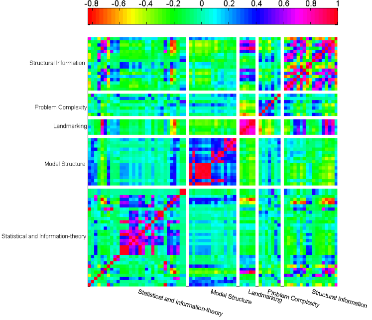
Figure 1: Correlation coefficients among different types of meta-features - 2.
Diverse base model construction
The literature has identified five different types of meta-features in the field of algorithm recommendation (See details in Appendix APPENDIX: Meta-features). These meta-features are extracted from different viewpoints of a classification problem independently. So it is reasonable to assume that, different types of meta-features are independent with each other. Fig. 1 gives the correlation coefficients among the five kinds of meta-features extracted from 1090 benchmark classification problems. From this figure, we can find that the correlation among different types of meta-features is usually quite low. This provides empirical evidence that different kinds of meta-features are independent of each other. Furthermore, it is more likely that different recommendation models constructed with these different types of meta-features will be independent/diverse.
3.2 Definitions of Accurate and Diverse Models
Let be an ensemble learning model constructed with base learning models {}, and () be the probability of to make an error prediction on a new coming instance. Then, for ensemble learning, an accurate learning model can be defined as follows.
Definition 3.2.
Accurate learning model. A base learning model () is accurate if and only if .
Definition 3.2 tells us that a base learning model is accurate if and only if its prediction error is less than 1/2. The rationality of this definition can be demonstrated as follows.
-
First, we construct another ensemble learning model over other base learning models {}, where each base model () has the identical probability to make an error prediction. And the probability is equal to the maximum value of {}. i.e, = ().
-
Then, by voting the predictions of the base learning models, we can get that since is constructed over a set of base models with lower possibility to make an error prediction. Suppose that the base learning models of the ensemble learning model ( or ) are independent of each other, we can get a discrete random variable following binomial distribution (, ), where indicates the number of models in {} which make an error prediction. According to binomial distribution, we can get:
(1) where denotes the smallest integer greater than (or equal to) .
-
Finally, according to Chernoff’s inequality [5], for binomial distribution (),
(2) where is the relative entropy between two Bernoulli distributions with parameters and , and defined as . Corresponding to ensemble learning model , , and so . Therefore, if and only if , by voting the predictions of {} as the prediction of , Eq. 2 will be always true. And will be bounded by . Moreover, in the case of , as increases, the value of will approach 0 since . That is, the more base learning models used, the smaller the probability of to make an error prediction. This will be a very good property for ensemble learning. In a word, all these conclusions will be true under ¡ . So in order to get an accurate ensemble learning model over {}, should be less than 1/2.
Without the independence/diversity22 2 In the field of ensemble learning, the independence of base learners is generally called diversity. among the base models {}, the random variable in Eq. 1 will not follow binomial distribution and further the Eq. 2 might be false. This will result in that might be non-convergent or converging too slowly. This phenomenon has been recognized in learner combination [15, 41]. And the diverse ensemble learner has a better potential to improve the accuracy than non-diverse ensemble learner [46, 14, 39]. Therefore, there will be a notable question: “How to define or evaluate the independence/diversity among the base learning models?”.
In the field of ensemble learning, it is usually difficult to evaluate the diversity between different learning models directly. Researchers usually resort to the prediction/classification results of the learning models on a given test data. There have been several metrics proposed based on the prediction results to assess the diversity between different models [39, 42, 15, 17]. These metrics can guide us to identify the diverse base models. Meanwhile, Kuncheva et al. [39] have stated that, in order to guarantee the improvement over the performance of base models, there exists a minimum threshold value for each of these diversity metrics to pick up the diverse base models for ensemble learning.
Following these ideas, suppose that and () are two different base models, and and are the prediction/classification results of and on a given test data set , we can give the definition of diverse learning model for ensemble learning as follows.
Definition 3.3.
Diverse learning model. Two base models and are diverse with each other if and only if , where is a function which computes the diversity between and based on and , and is a given minimum threshold.
In Definition 3.3, the computation of depends on the expression of the prediction results (e.g., ) of a learning model. There are three general expressions of the prediction results in the field of ensemble learning [39].
- 1.
- 2.
- 3.
For the numeric vector based expression, one of the assumptions is that a learning model outputs independent estimates of the posterior probabilities. However, this is usually not the case since all these posterior probabilities sum up to a constant 1. Moreover, not all the learning models can directly output the posterior probabilities of the class labels. In the field of ensemble learning, the researchers usually define the diversity function in terms of either class label or correct/incorrect decision [38, 17, 18, 40, 32, 26, 39]. In this paper, we propose a function, which makes full use of the prediction results and considers both of the class label and correct/incorrect decision, to pick up the diverse models for ensemble in next section.
3.3 Base Model Identification for Algorithm Recommendation
The definitions of accurate and diverse learning models in the previous section are stated for single-label learning and provide useful guidance for constructing ensembles over single-label learning problems. However, in this paper, we view algorithm recommendation as a multi-label learning problem and attempt to handle it by ensemble learning method.
Therefore, there will be a question: “How to identify the accurate and diverse base models for algorithm recommendation with respect to multi-label-based meta-data?” And this question can be answered by dividing it into the following ones.
-
Question 1: How to construct base recommendation models for ensemble on multi-label-based meta-data?
-
Question 2: How to identify an accurate recommendation model?
-
Question 3: How to identify a diverse recommendation model?
3.3.1 Answer to Question 1
This paper employs the frequently-used multi-label ensemble learning method, data transformation, to construct ensemble recommendation model on the multi-label-based meta-data. That is, we first transform the multi-label meta-data into multiple single-labeled meta-data, and then build recommendation models on these single-label meta-data as the base models of the ensemble.
Here, the process of multi-label meta-data transformation consists of two steps: i) in meta-feature space, a number of different sets of multi-label meta-data are generated with respect to different combinations of the existing meta-features (See details in Section 4.2); ii) in meta-target space, for each multi-label meta-data generated in i), multiple different sets of single-label meta-data are generated according to different labels of the meta-target in a specific way (See details in Section 4.3).
3.3.2 Answer to Question 2
Once we achieve the base models, it is straightforward to identify the accurate base models according to Definition 3.2. That is, for a given base model, if its classification error rate on test data is less than 1/2, it will be accurate, otherwise not.
3.3.3 Answer to Question 3
In order to identify the diverse models, according to Definition 3.3, two critical dimensions should be considered: one is to find a function to evaluate the diversity between two models, and the other is to set a proper threshold to pick up the diverse models. However, the existing researches usually just supply the function but no effective approach to preassign the threshold [39, 42, 15, 17].
In this paper, we present a statistical method that can not only quantify the diversity between two models but also adaptively set the threshold . Different from the existing diversity evaluation functions acting on the prediction results in terms of either the class labels or the direct/indirect decisions, the proposed diversity evaluation method concerning both of them, which will make full use of prediction results.
Suppose there are two different learning models and , and a data set with class labels {, , , } (), then we can construct a contingency table (see Table 1) based on the class labels and correct/incorrect decisions predicted by and on .
| Classified label | Total | ||||
|---|---|---|---|---|---|
| Total |
In Table 1, () is the number of test instances incorrectly classified as and by and , respectively. (), () and . is the total number of instances of which are incorrectly predicted by either or .
With this contingency table, we can get the diverse measure by Eq. 3. The greater the value of , the smaller the diversity between and .
| (3) |
where and .
According to the contingency table analysis, the joint frequency distribution of and predicted by and is , and and correspond to the marginal frequency distributions of and . The rationality of that can evaluate how strong the independence between and is demonstrated as follows.
- 1.
Suppose that and are independent of each other, the expected joint distribution of and would be . In Eq. 3, the numerator can also be represented as . Therefore, in the case that is independent of , will be quite close to 0 in practice.
- 2.
If the learner is positively related to , an instance being predicted as () by means that it is more likely that classifies the instance to as well. This will increase the value of , i.e., the elements on the main diagonal of the contingency table. Otherwise, if is negatively related to or independent with , the instance will be predicted as different classes by these two models. This will reduce the value of . So we can get that the value of can reflect the dependence of two different learners. That is why we define the metric by the elements on the main diagonal of the contingency table.
- 3.
The denominator of plays a role to limit the value of into the range . If the classification results on the test data are always identical, , so and achieves its maximum value 1. If and are independent of each other, will be 0 or quite near 0. And / means is negative/positive related to . The greater the value of , the stronger the dependence between and .
In practical application, the metric is estimated via the prediction results of the learning models on only a sample rather than the whole population. This might also be the reason that there needs a threshold in Definition 3.3. Therefore, we need to further understand the statistical significance of , including the statistical significance of and its confidence interval. And the confidence interval will be set as the threshold in Definition 3.3.
For this purpose, we need to find a statistic for significant test of . As we know, the distribution of the class labels predicted by a learner on a classification problem would follow either binomial () or multi-nominal () distribution. Both of binomial, multi-nominal distributions are derived from exponential family of distributions. Meanwhile, inspiring by the idea that the independence between two variables, which follow the well-known exponential distribution (i.e, normal distribution), is usually statistically tested by a -statistic, we attempt to employ a -statistic in Eq. 4 to test the significance of , and further determine whether two learning models and are independent with each other or not.
| (4) |
The statistic follows the Student’s t-distribution with freedom of degree under the null hypothesis that and are independent of each other. If the -statistic test accepts the null hypothesis under given significance level , we can conclude that the measure has no significant difference with 0, i.e., and are independent of each other.
According to Eq. 4, its inverse can be calculated as follow
| (5) |
where statistic follows student distribution with degree of freedom .
Let denote the critical value of student distribution with degree of freedom under a given significance level (e.g., = 0.05), then we can get the confidence interval of as . If calculated between two single learning models falls into this interval, we can conclude that these two models are statistically independent of each other under the given significance level . Based on this confidence interval, we can set the minimum threshold . And the diverse models can be detected by comparing with directly. That is, two models and are independent of each other if and only if .
4 Ensemble Learning Based Algorithm Recommendation
This section first shows the general view of the proposed ensemble learning-based recommendation method, then describes the process of model construction in detail.
4.1 General View
Firstly, different types of meta-features and the multi-labeled meta-target are collected over a set of historical classification problems; afterwards, by joining different combinations of these meta-features and the multi-labeled meta-target together, different sets of multi-label meta-data will be generated. Secondly, the base recommendation models are constructed on each of the generated multi-label meta-data. Thirdly, a multi-label ensemble learning recommendation model will be achieved by combining these base recommendation models together. Fig. 2 gives the general view of the proposed method which consists of three steps: i) meta-data preparation, ii) base recommendation model construction and iii) ensemble model construction.
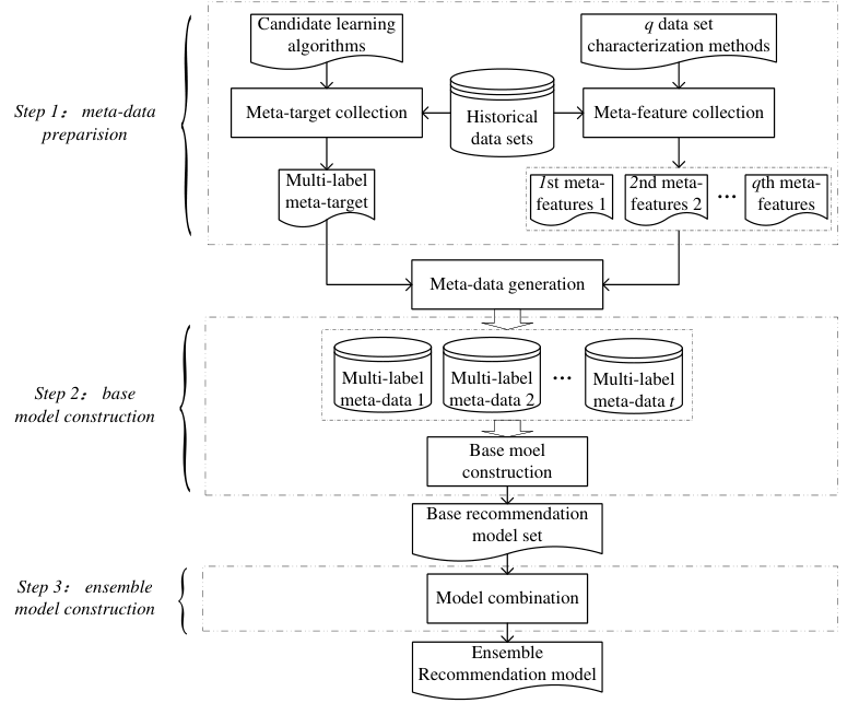
- 1)
Meta-data preparation
Meta-data is collected from a set of historical classification problems. i) For meta-feature collection, all the q different kinds of data characterization methods are utilized on the historical classification problems to get q groups of meta-features. ii) For meta-target collection, the appropriate algorithms of each historical classification problem are identified by statistically comparing all the candidate algorithms in terms of a given performance metric (such as, classification accuracy). And these appropriate algorithms form the multi-label-based meta-target.
Different types of meta-features reflect the properties of a classification problem in different viewpoints. Combinations of these meta-features will give us a more comprehensive understanding of the problem. Inspired by this idea, this paper attempts to construct the base recommendation models with respect to different combinations of these meta-features in a specific way. Firstly, q different sets of meta-features can be combined to generate combinations (See the generation process in Section 4.2). Then, by merging these combinations and the multi-labeled meta-target together, different sets of multi-label meta-data can be generated.
- 2)
Base recommendation model construction
For each multi-labeled meta data, firstly, the data transformation method is performed to transform the multi-labeled meta-data into multiple single-label meta-data, and then the base recommendation models will be generated from these single-label meta-data. The details of this process will be described in Section 4.3.
- 3)
Ensemble recommendation model construction
Once achieving the base recommendation models, the accurate and diverse base models are identified for constructing an ensemble recommendation model according to Section 3.3. For a new classification problem, the recommendations of these identified base models are combined in a specific way to form the recommended algorithms for the new problem. The detailed process of ensemble model construction will be introduced in Section 4.4.
4.2 Meta-data Preparation
Let be a set of candidate classification algorithms, be a set of historical classification problems, and be different data set characterization functions used for meta-feature extraction. denotes the meta-features extracted by () on the classification problem ().
Suppose that denotes a set of multi-label meta-instances, where is the meta-features extracted from the classification problem by the function(s) in , that is, , , , and here outputs all the possible combinations of the elements in . For example, let , then = {{}, {}, {}, {}, {}, {}, {}}; and represents the multi-label-based meta-target on and 1 or 0 indicates the algorithm is appropriate or inappropriate on .
It is noted that, there are many methods to generate different combinations of meta-features from the given kinds of meta-features. The combination function is chosen is because it can not only generate multiple different sets of meta-data for base model construction, but also help to find whether the combinations of different types of meta-features are better, and further discover the salient meta-features for algorithm recommendation.
With the combination function on different kinds of meta-features, we can generate different sets of meta-features and furthermore sets of multi-label meta-data.
4.3 Base Recommendation Model Construction
For each one of the sets of multi-label meta-data, the process to construct the base recommendation models is identical. This section will illustrate this process by taking one given multi-label meta-data as an example.

At first, the multi-label meta-data is transformed into multiple single-label data sets in meta-target space. The popular data transformation method, Binary Relevance (BR) [60], is performed. The BR method transforms into data sets which contain all the instances of labeled by whether algorithm is appropriate or not. This means that for each instance of , the corresponding instance of is . Fig. 3 shows the single-label data sets produced by BR on the multi-label meta-data .
Afterwards, recommendation models will be learned on these binary learning data sets by a specific classification algorithm (e.g, Decision Tree). These models constitute the base recommendation models on . Here, is a learning model which can output the probability () of the candidate algorithm being appropriate.
4.4 Combination of Base Recommendation Models
By combining the different types of meta-features, different sets of multi-label meta-data are achieved. After constructing base recommendation models on each one of the multi-label meta-data, we will get a learning model matrix , where denotes the model learned on the th data set transformed from th multi-label meta-data by BR method.
| (6) |
Let denote the th column of the matrix . According to the process of BR transformation method, consists of all the learning models with respect to the candidate algorithm . Thus, it is possible for us to construct the ensemble learning model improve the prediction of based on the models in .
According to Corollary 3.1, a useful practical strategy is to construct the ensemble from base models that are both accurate and diverse. Thus, ensemble model construction can be viewed as a process of selecting accurate and sufficiently diverse models from .
Algorithm 1 gives the filtering method on the models in . In this algorithm, besides , there are two other input variables and with respect to the models in , where () denotes the classification accuracy of on a validation data33 3 The validation data is drawn from the original meta-data and never used for model construction., and represents the outputs (i.e., predicted labels and correct/incorrect decisions) of on the validation data. records the filtering results, where and means that is filtered out/reserved for ensemble model construction.
Algorithm 1 consists of two filters: i) accuracy based filter (lines 2-3) and ii) diversity based filter (lines 5-14). The first filter is used to find out the accurate models. In this filter, the models whose classification accuracy being smaller than 1/2 are filtered out (i.e., set the corresponding flags in as 0) according to Definition 3.2 of accurate model. The second filter aims at finding out the diverse models. In this filter, if the between two specified models is greater than the predefined threshold according to Definition 3.3 of diverse model, the model with lower classification accuracy will be filtered out. Where the threshold is set according to Eq. 5.
With the help of Algorithm 1, we can get a flag matrix , where the column is achieved by applying Algorithm 1 on the models of the th column in the model matrix , (), and means the model is chosen for ensemble model construction.
| (7) |
Meanwhile, let be the th row of the model matrix , which consists of the models learned from the th multi-label meta-data. For a new coming classification problem , each model () predicts the probability to recommend the algorithm to . So we can further get a matrix of probabilities predicted by the model matrix on as follows.
| (8) |
With the predicted probability matrix and the flag matrix , the ensemble recommendation model will estimate the probability of the candidate algorithm that are appropriate on by the Eq. 9.
| (9) |
In Eq. 9, the denominator denotes the number of models chosen by Algorithm 1 on , i.e., the number of based models used for ensemble learning with respect to algorithm . The molecule of Eq. 9 can be viewed as a kind of weighted voting ensemble, where denotes the weight of model and it works if and only if , i.e., is picked up as a base model for ensemble learning.
Afterwards, the ensemble recommendation model can rank the candidate algorithms according to the estimated probabilitys . Meanwhile, the algorithm will be recommended as an appropriate one for if and only if is greater than a specific threshold (e.g., 1/2).
| Algorithm | |||||
|---|---|---|---|---|---|
| Probability value | 0.7 | 0.4 | 0.8 | 0.5 | 0.7 |
| Ranks | 2 | 5 | 1 | 4 | 3 |
| Ranks (considering ties) | 2.5 | 5 | 1 | 4 | 2.5 |
Meanwhile, these probabilitys can be further used to learn a ranking list of the candidate algorithms in on . The algorithm with the highest probability will be ranked first, the algorithm with the second highest probability will be ranked second, and so on. In case of ties, average ranks are assigned. This strategy can be illustrated by the example in Table 2 in which we give the estimated probability values of five candidate algorithms and corresponding ranks.
5 Experimental Study
This section presents the empirical evaluation of the proposed ensemble learning-based algorithm recommendation method. Because the main goal of this work is to demonstrate the effectiveness of combining heterogeneous meta-feature views, the experiments are organized around the following research questions:
- 1.
RQ1: Does the proposed ensemble recommendation model outperform individual recommendation models built from different meta-feature combinations?
- 2.
RQ2: Does combining heterogeneous meta-feature views improve recommendation performance compared with relying on a single view?
- 3.
RQ3: Does the proposed accuracy- and diversity-based filtering strategy improve the ensemble over simpler combination strategies?
- 4.
RQ4: Which types or combinations of meta-features contribute most to classification algorithm recommendation?
We first describe the experimental setup and then analyze the results in terms of these questions.
| ID | Name | # Attributes | # Instances | # Classes | ID | Name | # Attributes | # Instances | # Classes |
|---|---|---|---|---|---|---|---|---|---|
| 1 | anneal | 38 | 898 | 6 | 43 | liver-disorders | 6 | 345 | 2 |
| 2 | anneal.ORIG | 38 | 898 | 6 | 44 | lung-cancer | 56 | 32 | 3 |
| 3 | arrhythmia | 279 | 452 | 16 | 45 | lymph | 18 | 148 | 4 |
| 4 | audiology | 69 | 226 | 24 | 46 | mfeat-fourier | 76 | 2000 | 10 |
| 5 | australian | 14 | 690 | 2 | 47 | mfeat-karhunen | 64 | 2000 | 10 |
| 6 | autos | 25 | 205 | 7 | 48 | mfeat-morphological | 6 | 2000 | 10 |
| 7 | balance-scale | 4 | 625 | 3 | 49 | mfeat-zernike | 47 | 2000 | 10 |
| 8 | breast-cancer | 9 | 286 | 2 | 50 | molecular-biology_promoters | 58 | 106 | 2 |
| 9 | breast-w | 9 | 699 | 2 | 51 | monks-problems-1 | 6 | 556 | 2 |
| 10 | car | 6 | 1728 | 4 | 52 | monks-problems-2 | 6 | 601 | 2 |
| 11 | cleve | 11 | 303 | 2 | 53 | monks-problems-3 | 6 | 554 | 2 |
| 12 | cmc | 9 | 1473 | 3 | 54 | mushroom | 22 | 8124 | 2 |
| 13 | colic | 22 | 368 | 2 | 55 | nursery | 8 | 12960 | 5 |
| 14 | connect-4 | 42 | 13512 | 3 | 56 | optdigits | 64 | 5620 | 10 |
| 15 | credit-a | 15 | 690 | 2 | 57 | page-blocks | 10 | 5473 | 5 |
| 16 | credit-g | 20 | 1000 | 2 | 58 | pendigits | 16 | 10992 | 10 |
| 17 | crx | 15 | 690 | 2 | 59 | pima | 6 | 768 | 2 |
| 18 | cylinder-bands | 39 | 540 | 2 | 60 | postoperative-patient-data | 8 | 90 | 3 |
| 19 | dermatology | 34 | 366 | 6 | 61 | primary-tumor | 17 | 339 | 22 |
| 20 | diabetes | 8 | 768 | 2 | 62 | segment | 19 | 2310 | 7 |
| 21 | ecoli | 7 | 336 | 8 | 63 | shuttle-landing-control | 6 | 15 | 2 |
| 22 | flags | 29 | 194 | 8 | 64 | sick | 29 | 3772 | 2 |
| 23 | german | 15 | 1000 | 2 | 65 | solar-flare_1 | 12 | 323 | 2 |
| 24 | glass | 9 | 214 | 7 | 66 | solar-flare_2 | 12 | 1066 | 3 |
| 25 | haberman | 3 | 306 | 2 | 67 | sonar | 60 | 208 | 2 |
| 26 | hayes-roth | 4 | 132 | 3 | 68 | soybean | 35 | 683 | 19 |
| 27 | heart-c | 13 | 303 | 5 | 69 | spambase | 57 | 4601 | 2 |
| 28 | heart-h | 13 | 294 | 5 | 70 | spect | 22 | 267 | 2 |
| 29 | heart-statlog | 13 | 270 | 2 | 71 | spectrometer | 102 | 531 | 48 |
| 30 | hepatitis | 19 | 155 | 2 | 72 | splice | 61 | 3190 | 3 |
| 31 | horse-colic.ORIG | 21 | 368 | 2 | 73 | sponge | 45 | 76 | 3 |
| 32 | hypo | 23 | 3163 | 2 | 74 | tae | 5 | 151 | 3 |
| 33 | hypothyroid | 29 | 3772 | 4 | 75 | tic-tac-toe | 9 | 958 | 2 |
| 34 | ionosphere | 34 | 351 | 2 | 76 | trains | 32 | 10 | 2 |
| 35 | iris | 4 | 150 | 3 | 77 | transfusion | 3 | 748 | 2 |
| 36 | kdd_JapaneseVowels_1 | 14 | 5687 | 9 | 78 | vehicle | 18 | 846 | 4 |
| 37 | kdd_JapaneseVowels_2 | 13 | 4274 | 9 | 79 | vote | 16 | 435 | 2 |
| 38 | kdd_synthetic_control | 61 | 600 | 6 | 80 | vowel | 13 | 990 | 11 |
| 39 | kr-vs-kp | 36 | 3196 | 2 | 81 | waveform-5000 | 40 | 5000 | 3 |
| 40 | labor | 16 | 57 | 2 | 82 | wine | 13 | 178 | 3 |
| 41 | led7 | 7 | 3200 | 10 | 83 | yeast | 7 | 1484 | 10 |
| 42 | letter | 16 | 20000 | 26 | 84 | zoo | 17 | 101 | 7 |
5.1 Experimental Setup
To evaluate the effectiveness and practical applicability of the proposed ensemble learning-based algorithm recommendation method, we use the following experimental setup.
5.1.1 Benchmark Classification Problem
We use 84 widely used public classification problems from the UCI repository44 4 http://archive.ics.uci.edu/ml/datasets.html. in the experiments. Table 3 shows the statistical summary of these problems in terms of the number of attributes, the number of instances and the number of classes.
Moreover, in order to guarantee the reliability and soundness of the conclusion, more classification problems should be employed. Thus, with the help of the problem generation method, Datasetoids, which was proposed in [57] and aimed to obtain a large number of classification problems for algorithm recommendation [50, 49, 27, 51], we extend the 84 publicly UCI classification problems into 1090 (84 data sets and 1006 datasetoids) different classification problems. The Datasetoids method generates the new classification problems by exchanging role of each nominal attribute with that of a target concept, i.e., viewing the nominal attribute as the new target concept.
5.1.2 Meta-feature Collection
Five different types of meta-features are extracted from the 1090 classification problems. They are i) the statistical and information-theory based, ii) the model structure based, iii) the landmarking based, iv) the problem complexity based and v) the structural information based. See Appendix APPENDIX: Meta-features for the details.
5.1.3 Meta-target Collection
Meta-target tells us the appropriate candidate algorithms for each of the 1090 classification problems. Next, we introduce the candidate classification algorithms in the experiments and how to identify the appropriate algorithms for a given classification problem.
- 1.
Candidate classification algorithms
To improve the generality of the experimental results, 13 different types of classification algorithms are selected as candidates.
These algorithms include i) the probability based algorithm Bayes Network; ii) tree based algorithms C4.5, RandomTree and RandomForest; iii) rule-based algorithms PART, Ripper and NNge; iv) Gaussian function based algorithm RBFNetwork, and v) support vector machine based algorithm SMO.
Besides the above nine single classification algorithms, we also include two types of well-known ensemble classification algorithms: Boosting and Bagging. They are applied with the base classifiers Naive Bayes (NB) and C4.5, respectively.
- 2.
Appropriate algorithm identification
The multi-label-based meta-target indicating the appropriate algorithms for a classification problem can be expressed in terms of a binary value vector , where means that the corresponding candidate algorithm () is appropriate. The appropriate algorithms are identified by their performance metrics (i.e., classification accuracy) on as follows.
- (a)
Process of classification accuracy estimation on
In order to get a stable estimation of classification accuracy of the candidate algorithms on , -fold stratified cross-validation is performed as the following steps. i) The problem is randomly split into ten mutually exclusive subsets of equal size, and . ii) and () are used as the training and test sets, respectively. Each algorithm () is trained on , and its classification accuracy is estimated on . iii) Repeat i) and ii) five times on whose instances are randomly re-ordered. Afterwards, for each candidate algorithm (), we will get a vector with 50 classification accuracies.
- (b)
Binary-valued based meta-target identification
In order to identify the truly appropriate algorithms from 13 candidate algorithms according to the collected performance sets , , , on , the statistical algorithm selection is a reasonable and commonly-used approach [48].
To find out the superior algorithms from three or more candidate algorithms, the traditional statistical methods usually resort to multiple paired t-tests. However, it has been proved that this approach usually leads to high Type I error.55 5 The probability that we make a mistake to reject the null hypothesis, i.e., a misjudgement to say there exists significant difference but actually does not.
For solving this problem, we turn to the multiple comparison procedure. The multiple comparison procedure is a statistical test technique which helps us compare three or more groups of metrics (e.g., classification accuracy) while controlling the probability to make the statistical Type I error [48]. Moreover, it allows us to concern with a set of candidate algorithms not significantly different from the best one rather than a single algorithm. Therefore, the multiple comparison procedure is an effective method for multi-labeled meta-target collection.
Therefore, in our experiment, as suggested in [16], we employ the non-parametric multiple comparison procedure, Friedman followed by Holm’s procedure test, to obtain the binary-value based meta-target for the problem according to as follows.
- i.
Applying Friedman test on , the null hypothesis of Friedman test is there does not exist significant difference among these 13 algorithms. If the result of the test support the null hypothesis, all these 13 algorithms will be viewed as the appropriate ones. This means that of (), . And the multiple comparison procedure is over.
- ii.
Otherwise, there will exist significant difference among these candidate algorithms. In this case, we should apply the post-hoc Holm’s procedure test to further find the real appropriate algorithms. At first, the algorithm with the highest average classification accuracy is picked up as a reference. And the Holm’s procedure test is performed to identify the appropriate algorithms from the rest ones. The algorithms that have no significant differences with the reference are viewed as the appropriate algorithms. Of course, the reference is an appropriate one as well. Afterwards, for each value in , if the corresponding algorithm is identified as an appropriate one, , otherwise, .
- i.
- (a)
5.1.4 Recommendation model construction
The proposed ensemble multi-label learning-based recommendation model combines a set of base models constructed on different sets of meta-data. In order to demonstrate whether the proposed ensemble method is competitive in constructing the recommendation model, we compare the performance of the ensemble recommendation model with those of the base models.
When constructing the base model on a given multi-label meta-data, the data transformation method BR first transforms the multi-labeled meta-data into multiple single-label meta-data, and then the well-known classification algorithm, decision tree, is applied on these single-label meta-data to get the base recommendation models. The tree-based learner being used is due to the fact that the it is quite effective to be explored and has good explanation.
Moreover, one critical factor affecting the performance of ensemble learning is that whether the base models are accurate and diverse. In order to testify how the accurate and diverse base models affect the recommendation performance of the ensemble recommendation method in our experiment, we compare the recommendations of the ensemble models constructed with respect to four different sets of base models, including i) all learned base models ii) only accurate base models, iii) only diverse base models and iv) both of accurate and diverse models.
5.1.5 Metrics to Evaluate Recommendation Models
In order to measure the performance of the recommendation model, two metrics which have been used to evaluate the multi-label methods are defined as follows.
For a given classification problem , let represent the recommended rank list of candidate algorithms on . Meanwhile, suppose that () indicates whether a candidate algorithm is truly appropriate (i.e., ) or not (i.e., ) on , be the set of indexes of truly appropriate algorithms and be the set of indexes of the inappropriate algorithms on .
Ranking Loss represents the number of times that inappropriate algorithms are ranked higher than the truly appropriate algorithms. Ranking loss of the recommended rank list is defined as follow.
Definition 5.1.
Ranking Loss
| (10) |
For algorithm recommendation results in the form of ranking, in a practical application, the 1st ranked algorithm is usually in favor, then the 2nd ranked one, and so forth. Therefore, it is natural for the users to ask that whether the top ranked algorithms are true appropriate or not. In this case, precision of ranking results, which has been widely-used in the field of information retrieval to measure whether the top ranked records are true relevant [6], is employed as a measure to evaluate how well the algorithm-ranking-based recommendation results.
Precision at to measure the accuracy of the top recommended algorithms on problem is calculated by Eq. 11.
| (11) |
With precision at , average precision [6] to measure the accuracy of the recommendation result on problems is defined as follows.
Definition 5.2.
Average Precision
| (12) |
where denotes the number of the candidate algorithms, and is a binary function to indicate whether the th ranked algorithm in is truly appropriate () or not (). The numerator represents the number of the truly appropriate algorithms on .
5.1.6 Recommendation method validation
After the multi-label meta-data with 1090 instances is acquired, -fold cross-validation is applied to to empirically evaluate the proposed algorithm recommendation method as follows.
It is important to note that the meta-level evaluation uses held-out classification problems. During each outer split, the recommendation model is trained only on the meta-instances in the training fold, the base-model filtering step uses only the validation fold, and the final recommendation performance is evaluated only on the test fold. The meta-targets of the test-fold problems are used only for evaluation and are not used to train or select the recommendation model.
- 1.
is randomly divided into 10 sub data sets in the same size , and ().
- 2.
Each sub data set is viewed as the test data , and the union of rest sub data sets are randomly divided into two equal-size parts: training data and valid data .
- 3.
- 4.
Combine the filtered base recommendation models to form the ensemble recommendation model, and evaluate the ensemble model in terms of Ranking Loss and on the test data .
- 5.
Repeat the above four steps five times, for each time, the order of the 1090 instances in is rearranged randomly.
5.2 Results and Analysis
This section compares the proposed ensemble recommendation model with individual base recommendation models in terms of Ranking Loss, Average Precision, and top-ranked recommendation precision. The analysis emphasizes empirical behavior across the 1,090 classification problems rather than relying on theoretical guarantees.
For the sake of understanding the results, we denote the different combinations of the five different types of meta-features in Table 4, where numbers “1”, “2”, “3”, “4” and “5” appearing in column “Comment” represent five different kinds of meta-features, respectively.
| Notation | Comment | Notation | Comment | Notation | Comment | Notation | Comment |
|---|---|---|---|---|---|---|---|
| 1 | {1} | 9 | {1,5} | 17 | {1,2,4} | 25 | {3,4,5} |
| 2 | {2} | 10 | {2,3} | 18 | {1,2,5} | 26 | {1,2,3,4} |
| 3 | {3} | 11 | {2,4} | 19 | {1,3,4} | 27 | {1,2,3,5} |
| 4 | {4} | 12 | {2,5} | 20 | {1,3,5} | 28 | {1,2,4,5} |
| 5 | {5} | 13 | {3,4} | 21 | {1,4,5} | 29 | {1,3,4,5} |
| 6 | {1,2} | 14 | {3,5} | 22 | {2,3,4} | 30 | {2,3,4,5} |
| 7 | {1,3} | 15 | {4,5} | 23 | {2,3,5} | 31 | {1,2,3,4,5} |
| 8 | {1,4} | 16 | {1,2,3} | 24 | {2,4,5} |
-
“1” = statistical and information-theory based meta-features; “2” = model structure based meta-features; “3” = Landmarking Based meta-features; “4” = problem complexity based meta-features and “5” = structural information based meta-features.
5.2.1 Comparison on Ranking Loss
Fig. 4 compares the ensemble learning-based recommendation model with the models constructed on different combinations of meta-features in terms of Ranking Loss. The smaller the Hamming Loss, the better the corresponding recommendation model. In this figure, a separate box is produced by the “box plot” for each recommendation model according to its Ranking Loss values evaluated on the meta-data. The notch of each box denotes the comparison intervals of the median value of Ranking Loss estimated on the corresponding recommendation model. Two medians are significantly different at the 5% significance level if their intervals do not overlap. And the box marked as “En” denotes the ensemble learning-based recommendation model, and the th box denotes of the recommendation model constructed on the th combination of meta-features in Table 4. The same representation can be found in Figs. 5and 6. From Fig. 4, we can observe that:
- 1.
The Ranking Losses of different recommendation models are different. And the differences among some models are significant. This means that the recommended rankings of candidate algorithms vary with different recommendation models. Meanwhile, no matter under which kind of combinations of meta-features in Table 4, the recommendation model constructed on the combined meta-features performs equally or better than the single kind of meta-features. The reason is that different kinds of meta-features characterize the classification problems in different viewpoints and will be relatively complemented, so the combinations can give us more comprehensive understanding of the problem. Furthermore, it is possible to construct more precise decision tree model to distinguish the appropriate and inappropriate candidate algorithms.
- 2.
The Ranking Loss of ensemble learning-based model (i.e., the last box) is the lowest. And it is significantly smaller than that of any other recommendation model (i.e., any box numbered by ). For the other 31 recommendation models, the smallest/greatest median value of Ranking Loss is 0.2483/0.3047. However, by combining these 31 recommendation models together to form the ensemble recommendation model, the median value of Ranking Loss is only 0.17, and outperforms the best base recommendation model by 31.53%. This means that the proposed ensemble learning method is more effective to estimate the ranking of the candidate algorithms.
5.2.2 Comparison on Precision
Fig. 5 shows the comparison results of different recommendations in terms of average precision. From this figure, we can get that:
- 1.
The Average Precision varies with different recommendation models. For single kind of meta-features corresponding to the first five recommendation models, there exists distinctly significant difference among the Average Precision, such as the Average Precision of the models constructed on the statistic and information theory and structural information based meta-features is significantly greater than that of the models constructed on other three kinds of meta-features.
For the models constructed on the different combinations of the five kinds of meta-features, their Average Precisions are either statistically equal to or greater than that of model constructed on the corresponding single kind of meta-features. For example, the 10th box corresponds to the Average Precision of the model constructed on the combinations of 2nd and 3rd meta-features. And its median is statistically greater than that of either the 2nd or 3rd box.
- 2.
The average precision of ensemble learning-based model, which is achieved by integrating the 31 recommendation models together, is the highest and statistically better than that of any of the other 31 recommendation models. For the 31 base recommendation models, the greatest/smallest median value of Average Precision is 0.7097/0.6637. However, by combining these 31 base recommendation models together to form the ensemble recommendation model, the median value of Average Precision can be up to 0.7785, and outperforms the best base recommendation model by 9.69%. This indicates that combining the recommendation models constructed on different sets of meta-features together is an effective way to construct the more accurate recommendation model.
Besides the average precision, the user might be interested on the precision of the top ranked algorithm. That is, whether the first recommended algorithm is one of the truly appropriate algorithms. This can be measured by the metric Precision(1) of the recommendation model. Fig. 6 shows the Precision(1) of different recommendation models. From Fig. 6, we can observe that, the Precision of the top ranked algorithm recommended by different recommendation models is different. For the 31 base recommendation models, the greatest/smallest median value of Precision(1) is 0.6697/0.5871. However, by combining these 31 base recommendation models together to form the ensemble recommendation model, the median value of Precision(1) can be up to 0.7615, and outperforms the best base recommendation model by 13.71%.
In summary, no matter in terms of either Average Precision or Precision(1), the proposed ensemble learning-based algorithm recommendation method is significantly better than the existing recommendation models.
5.2.3 Sensitive Analysis of Ensemble Recommendation Model
A central empirical question is whether accuracy-based and diversity-based base-model filtering actually improves the ensemble recommendation model. This section therefore analyzes the contribution of these two factors to the final recommendation performance. Fig. 7 shows the sensitive analyses of these two aspects on the recommendation models in terms of Ranking Loss, Average Precision, Precision(1) and the number of base models used for ensemble learning, respectively. In this figure, i) “all” represents that all the 31 base recommendation models are used for ensemble model construction; ii) “accurate” denotes the 31 base models are only filtered by the Definition 3.2 of accurate learning model; iii) “diverse” denotes the 31 base models are only filtered by the Definition 3.3 of diverse learning model and iv) “accurate & diverse” means that the 31 base models are filtered by both Definitions 3.2 and 3.3.
From Fig. 7, we can get that:
- 1.
For each sub-figure, the four kinds of recommendation models can be grouped into two categories according to the box plots of their performance metrics. The models marked as “all” and “accurate” have statistically equal performance, and the other two models perform statistically equally as well.
This is because that during the base recommendation model construction, for most of the single-label learning problems transformed from the multi-label meta-data by BR transformation method, the classification accuracy of decision tree on them is greater than 0.5. Therefore, the classification accuracy based filter can just filter out quite a few decision trees. That mean, for recommendation models marked as “all” and “accurate”, the decision trees used for model construction are quite in common. This leads to that the performance of recommendation models marked as “all” and “accurate” are quite similar. Similarly, since the difference among the construction of models marked as “diverse” and “accurate & diverse” derives from the classification accuracy based filter, their performance is similar. This can be also confirmed by the Fig. 7 (d) showing the average number of trees used for ensemble learning-based algorithm recommendation. The recommendation models marked as “all” and “accurate” are constructed based on almost the same number of decision trees. So the same as the recommendation models marked as “diverse” and “accurate & diverse”.
- 2.
Since that the most decision trees used for algorithm recommendation model constructed are accurate according to Definition 3.2 of accurate learning model, the proposed ensemble learning-based algorithm recommendation method focuses on finding out the diverse base learning models. According to Fig. 7, after filtering out the decision trees by Definition 3.3 of diverse base model, we get better ensemble learning-based recommendation models with less number of decision trees. Such as, the model marked as “diverse” with diversity based filter outperforms the model marked as “all” in terms of all the performance metrics Ranking Loss, Average Precision and Precision(1); and the model marked as “accurate & diverse” is better than the model marked as “accurate”. This indicates that in Eq. 3 is a good choice to evaluate the diversity between different base models and can be used to detect diverse base models for ensemble learning based algorithm recommendation.
In summary, by the sensitive analysis of two important aspects (including accurate and diverse base learning models) in ensemble learning model construction, we can conclude that, for classification algorithm recommendation, the proposed definitions of accurate and diverse learning models are effective to find out a good set of base recommendation models to construct better ensemble recommendation model.
6 Conclusions
This paper proposed a multi-view ensemble meta-learning method for automatically recommending appropriate classification algorithms for new classification problems. The method formulates algorithm recommendation as a multi-label learning problem, reflecting the practical observation that multiple algorithms may be statistically competitive on the same data set.
The main contribution of the paper is empirical. Unlike existing recommendation methods that usually build a single model from one type of meta-feature, the proposed method constructs base recommendation models from different combinations of heterogeneous meta-feature groups and combines them through an accuracy- and diversity-aware ensemble strategy. This design allows the recommendation model to exploit complementary information from multiple views of the data.
We evaluated the proposed method on 1,090 benchmark classification problems, 13 candidate classification algorithms, and five types of meta-features. The experimental results show that the ensemble learning-based recommendation model improves ranking loss, average precision, and top-ranked recommendation precision compared with individual recommendation models. The sensitivity analysis further shows that both accuracy-based and diversity-based base-model filtering contribute to the final recommendation performance.
The proposed framework has several limitations. First, the current implementation uses Binary Relevance to transform the multi-label recommendation problem, which does not explicitly model dependencies among candidate algorithms. Second, the diversity threshold is derived from an approximate statistical criterion and may not be optimal for all data distributions. Third, the empirical study uses classification accuracy as the primary performance measure; other criteria, such as training time, inference cost, robustness, and interpretability, may lead to different recommendations. Finally, the current experiments focus on traditional classification algorithms, and extending the framework to modern AutoML pipelines and deep learning models is an important direction for future work.
Future work will investigate more flexible model-combination strategies, stronger multi-label transformation methods such as classifier chains or RAKEL, additional meta-feature representations, and broader algorithm-selection settings.
APPENDIX: Meta-features
Meta-features are measures extracted from a classification problem to describe its properties. These measures map each classification problem into a real-valued vector in the domain through the extraction function .
Meta-feature extraction is one of the most challenging aspects of algorithm recommendation. In principle, any measure that reflects a property of a classification problem can be viewed as a meta-feature. In practice, however, useful meta-features should be (i) related to the performance of classification algorithms, (ii) easy to compute, and (iii) applicable to different classification problems.
Researchers have proposed several data set characterization methods that describe classification problems from different perspectives. These meta-features can be broadly grouped into the following five categories.
| Measures | Definitions |
|---|---|
| Ins.Num | Number of instances |
| Attr.Num | Number of Attributes |
| Target.Num | Number of target concept values |
| Target.Min | Proportion of minority target |
| Target.Max | Proportion of majority target |
| Pro.Bin | Proportion of binary attributes |
| Pro.Nom | Proportion of nominal attributes |
| Pro.Num | Proportion of numeric attributes |
| Pro.MissIns | Proportion of instances with missing values |
| Pro.MissValues | Proportion of missing values |
| Mean.Geo | Geometric mean |
| Mean.Harm | Harmonic mean |
| Mean.Trim | Trim mean excluding the highest and lowest 5% |
| Mad | Mean absolute deviation |
| Var | Variance |
| Std | Standard deviation |
| Prcitile | Percentile 75% |
| Int.Range | Interquartile range |
| Prop.AttrWithOutlier | Proportion of numerical attributes with outliers over all numerical attributes |
| Skewness | Skewness of data based on numerical attributes |
| Kurtosis | Kurtosis of data based on numerical attributes |
| Max.eig | Maximum eigenvalue |
| Min.eig | Minimum eigenvalue |
| Can.corr | Canonical correlation |
| Grav.cent | Center of gravity |
| MeanAbsCoef | Mean absolute coefficient of attribute pairs |
| Entropy of classes | |
| Mean entropy of nominal attributes | |
| Mean mutual information of classes and attributes based on nominal attributes | |
| En.attr | Equivalent number of attributes |
| Ns.ratio | Noise-signal ratio |
| Measures | Definitions |
|---|---|
| Tree.Height | Height of tree (also referred as to number of levels in tree) |
| Tree.Wdith | Width of tree |
| Node.Num | Number of nodes in tree |
| Leaf.Num | Number of leaves in tree |
| Level.Max | Maximum number of nodes at one level |
| Level.Mean | Mean of the number of nodes on levels |
| Level.Dev | Standard deviation of the number of nodes on levels |
| Branch.Long | Length of the longest branch |
| Branch.Short | Length of the shortest branch |
| Branch.Mean | Mean of the branch lengths |
| Branch.Dev | Standard deviation of the branch lengths |
| Attr.Min | Minimum occurrence of attributes |
| Attr.Max | Maximum occurrence of attributes |
| Attr.Mean | Mean of the number of occurrences of attributes |
| Attr.Dev | Standard deviation of the number of occurrences of attributes |
| Measures | Definitions |
|---|---|
| Bound.Len | Length of class boundary |
| Adherence.Prop | Proportion of retained adherence subsets |
| Intra/Inter.Ratio | Ratio of average intra/interclass nearest neighbors |
| NN.Nonlinerity | Nonlinearity of Nearest Neighbors classifier |
| Linear.Nonlinerity | Nonlinearity of linear classifier |
| Fisher.Ratio | Maximum Fisher’s discriminant ratio |
| Ins/Attr | Training set size relative to feature space dimensionality |
- 1.
Statistical and Information-theory Based Measures
The statistical and information-theory based measures are the most widely-used in the field of classification algorithm recommendation [10, 58, 29, 1, 25, 23]. The prominent examples based on these measures are the projects ESPRIT Statlog (1991-1994) and METAL (1998-2001). These measures generally include the data set characteristics such as, number of features, number of instances, number of target concepts, ratio of instances to features, ratio of missing values, ratio of binary features, entropy of the target concept, information gain between the feature and the target concept, and correlation coefficient between features, etc. See Table 7 for details.
- 2.
Model Structure Based Measures
Firstly, a classification problem is represented in a special data structure embedding the complexity of the problem. Then, the characteristics of the structure are exploited to describe the classification problem.
In the field of algorithm recommendation, the induced decision tree is a well-known and commonly-used structure to model a classification problem. Bensusan [8] proposed to capture the information from the induced decision tree for describing the classification complexity. He extracted ten measures from the decision tree, such as the ratio of the number of nodes to the number of features, the ratio of the number of nodes to the number of instances, etc. Afterwards, Peng et al. [45] re-analyzed the characterization of decision trees, and proposed some new measures to characterize the structural properties of decision trees. See Table 7 for details.
- 3.
Landmarking Based Measures
This kind of measures falls within the concept of landmarking [47, 7, 33, 20]. This idea was proposed based on the assumption that the performance of the candidate algorithms could be predicted by the performance of a set of simple classifiers (also called landmarkers). So the performance (e.g., accuracy) of these landmarkers is used to describe a classification problem. Evidently, this kind of measures is closely related to the choice of landmarkers. In practice, it should be ensured that the chosen landmarkers have significant differences in terms of learning mechanism. Following the suggestions in [7, 47], the following six classifiers are selected as the landmark learners: i) Naive Bayes, ii) 1-NN (Nearest Neighbor), iii) Elite 1-NN, iv) a decision node tree, v) a random chosen node tree and vi) the worst node tree. Where the last three classifiers can be achieved based on the well-known classification algorithm C4.5.
- 4.
Problem Complexity Based Measures
The problem complexity based measures focus on the description of the geometrical complexity of the classification problem and emphasize the geometrical characteristics of the distributions of the classes by analyzing the source of difficulty in solving a classification problem [9, 30, 22, 31]. The measures reflecting the way in which different classes are separated or interleaved (and being relevant to classification performance) are identified as the measurement of the problem’s complexity. Such as Fisher’s discriminant ratio, the percentage of instances in the problem that linear the class boundary, and the nonlinearity of linear/non-linear classification algorithm, etc. See Table 7 for details.
- 5.
Structural Information Based Measures
Recently, Song et al. proposed a novel data characterization method to facilitate the algorithm recommendation [59]. The method utilizes structural information based feature vectors to characterize the classification problems, which is quite different from the existing ones. Specially, the two feature vectors, one-item feature vector and two-item feature vector, are extracted from a given classification problem. These two vectors consist of the frequencies of one-item sets and two-item sets, respectively. Afterwards, the minimum, 1/8 quantile, 2/8 quantile, 3/8 quantile, 4/8 quantile, 5/8 quantile, 6/8 quantile, 7/8 quantile and maximum are computed for these two vectors and form the final set of data set characteristics.
References
- [1] (1992) Generalizing from case studies: a case study. In Proceedings of the Ninth International Conference on Machine Learning, pp. 1–10. Cited by: item 1.
- [2] (2018) A case-based meta-learning and reasoning framework for classifiers selection. In Proceedings of the 12th International Conference on Ubiquitous Information Management and Communication, pp. 1–6. Cited by: §1, §2.
- [3] (2006) On learning algorithm selection for classification. Applied Soft Computing 6 (2), pp. 119–138. Cited by: §1, §1, §2, §3.1.
- [4] (2006) A meta-learning approach to automatic kernel selection for support vector machines. Neurocomputing 70 (1), pp. 173–186. Cited by: §2, §3.1.
- [5] (1989) Tutorial on large deviations for the binomial distribution. Bulletin of Mathematical Biology 51 (1), pp. 125–131. Cited by: item 3.
- [6] (1999) Modern information retrieval. ACM press New York. Cited by: §5.1.5, §5.1.5.
- [7] (2000) Casa batlo is in passeig de gracia or landmarking the expertise space. In Proceedings of the ECML’2000 workshop on Meta-Learning: Building Automatic Advice Strategies for Model Selection and Method Combination, pp. 29–47. Cited by: item 3, §1, §2, §2, item 1.
- [8] (1998) God doesn’t always shave with occam’s razor - learning when and how to prune. In Proceedigs of the 10th European Conference on Machine Learning, pp. 119–124. External Links: ISBN 3-540-64417-2 Cited by: item 2, §1, §1, §2, §2, item 1.
- [9] (2005) Domain of competence of XCS classifier system in complexity measurement space. IEEE Transactions on Evolutionary Computation 9 (1), pp. 82–104. Cited by: item 4, §2.
- [10] (2003) Ranking learning algorithms: using IBL and meta-learning on accuracy and time results. Machine Learning 50 (3), pp. 251–277. Cited by: item 1, §1, §1, §1, §2, §2, §2, item 1, §3.1.
- [11] (1994) Characterizing the applicability of classification algorithms using meta-level learning. In Proceedings of European Conference on Machine Learning, pp. 83–102. Cited by: §3.1.
- [12] (2000) A comparison of ranking methods for classification algorithm selection. pp. 63–75. Cited by: §2.
- [13] (1993) Addressing the selective superiority problem: automatic algorithm/model class selection. In Proceedings of the Tenth International Conference on Machine Learning, pp. 17–24. Cited by: §3.1.
- [14] (2005) Diversity creation methods: a survey and categorisation. Information Fusion 6 (1), pp. 5–20. Cited by: §3.2.
- [15] (2000) Diversity versus quality in classification ensembles based on feature selection. In The European Conference on Machine Learning and Principles and Practice of Knowledge Discovery in Databases, pp. 109–116. Cited by: §3.2, §3.2, §3.3.3.
- [16] (2006) Statistical comparisons of classifiers over multiple data sets. Journal of Machine Learning Research 7, pp. 1–30. Cited by: item 2b.
- [17] (2000) An experimental comparison of three methods for constructing ensembles of decision trees: bagging, boosting, and randomization. Machine Learning 40 (2), pp. 139–157. Cited by: item 2, §3.2, §3.2, §3.3.3.
- [18] (2000) Ensemble methods in machine learning. In Multiple Classifier Systems, pp. 1–15. Cited by: §2, item 1, item 2, §3.1, §3.1, §3.2.
- [19] (2002) Ensemble learning. The Handbook of Brain Theory and Neural Networks, pp. 405–408. Cited by: §2, item 1, §3.1, §3.1.
- [20] (2004) The characterization of classification problems by classifier disagreements. In Proceedings of the 17th International Conference on Pattern Recognition, Vol. 1, pp. 140–143. Cited by: item 3, §2, §2, item 1.
- [21] (2004) Is combining classifiers with stacking better than selecting the best one?. Machine Learning 54 (3), pp. 255–273. Cited by: §2.
- [22] (2009) Estimation of classification complexity. In Proceedings of International Joint Conference on Neural Networks, pp. 764–770. Cited by: item 4, §2, §2, item 1.
- [23] (1998) Using a data metric for preprocessing advice for data mining applications. In Proceedings of the European Conference on Artificial Intelligence, pp. 430–434. Cited by: item 1, §1, §2, §2, item 1.
- [24] (2007) Random k-labelsets: an ensemble method for multilabel classification. In 18th European Conference on Machine Learning (ECML 2007), pp. 406–417. Cited by: §2.
- [25] (2000) Cascade generalization. Machine Learning 41 (3), pp. 315–343. Cited by: item 1, §1, §2, §2, item 1.
- [26] (2001) Design of effective neural network ensembles for image classification processes. Image and Vision Computing 19, pp. 699–707. Cited by: item 3, §3.2.
- [27] (2012) Identifying characteristics of seaports for environmental benchmarks based on meta-learning. Knowledge Management and Acquisition for Intelligent Systems, pp. 350–363. Cited by: §5.1.1.
- [28] (1990) Neural network ensembles. IEEE Transactions on Pattern Analysis and Machine Intelligence 12, pp. 993–1001. Cited by: §3.1.
- [29] (1994) Methods for comparison. pp. 107–124. Cited by: item 1.
- [30] (2002) Complexity measures of supervised classification problems. IEEE Transactions on Pattern Analysis and Machine Intelligence 24 (3), pp. 289–300. Cited by: item 4, §1, §2, §2, item 1.
- [31] (2000) Complexity of classification problems and comparative advantages of combined classifiers. Multiple Classifier Systems, pp. 97–106. Cited by: item 4, §2.
- [32] (1998) The random subspace method for constructing decision forests. IEEE Transactions on Pattern Analysis and Machine Intelligence 20 (8), pp. 832–844. External Links: ISSN 0162-8828, Document Cited by: item 3, §3.2.
- [33] (2000) Statistical pattern recognition: a review. IEEE Transactions on Pattern Analysis and Machine Intelligence 22 (1), pp. 4–37. Cited by: item 3, §2, §2, item 1.
- [34] (2004) On data and algorithms: understanding inductive performance. Machine Learning 54 (3), pp. 275–312. Cited by: §2, §3.1.
- [35] (2002) Algorithm selection via meta-learning. Ph.D. Thesis. Cited by: §1, §2, §3.1.
- [36] (2020) A literature survey and empirical study of meta-learning for classifier selection. IEEE Access 8, pp. 10262–10281. Cited by: §1, §2.
- [37] (1995) Statlog: comparison of classification algorithms on large real-world problems. Applied Artificial Intelligence an International Journal 9 (3), pp. 289–333. Cited by: §3.1.
- [38] (1996) Bias plus variance decomposition for zero-one loss functions. In International Conference on Machine Learning, pp. 275–283. Cited by: item 2, §3.2.
- [39] (2003) Measures of diversity in classifier ensembles and their relationship with the ensemble accuracy. Machine Learning 51 (2), pp. 181–207. Cited by: §3.2, §3.2, §3.2, §3.2, §3.3.3.
- [40] (2003) Limits on the majority vote accuracy in classifier fusion. Pattern Analysis and Applications 6, pp. 22–31. External Links: Document Cited by: item 3, §3.2.
- [41] (2000) Classifier combinations: implementations and theoretical issues. In Multiple Classifier Systems, pp. 77–86. Cited by: §3.2.
- [42] (2013) Automatic selection of classification learning algorithms for data mining practitioners. Intelligent Data Analysis 17 (4), pp. 665–678. Cited by: §3.2, §3.3.3.
- [43] (1999) Cleansing data for mining and warehousing. In Proceedings of the 10th International Conference on Database and Expert Systems Applications, pp. 751–760. Cited by: item 1.
- [44] (2010) A Triple-Random Ensemble Classification Method for Mining Multi-label Data. In IEEE International Conference on Data Mining, pp. 49–56. External Links: Document Cited by: §2.
- [45] (2002) Improved dataset characterisation for meta-learning. In Discovery Science, pp. 193–208. Cited by: item 2, §1, §1, §2, §2, item 1, §3.1.
- [46] (2005) Estimating the potential for combining learning models. In Proceedings of the ICML workshop on meta-learning, pp. 68–75. Cited by: §3.2.
- [47] (2000) Meta-learning by landmarking various learning algorithms. In Proceedings of the Seventeenth International Conference on Machine Learning, pp. 743–750. Cited by: item 3, §1, §1, §2, §2, item 1, §3.1.
- [48] (2002) Multiple comparison procedures applied to model selection. Neurocomputing 48, pp. 155–173. Cited by: item 2b, item 2b.
- [49] (2011) Uncertainty sampling methods for selecting datasets in active meta-learning. In The 2011 International Joint Conference on Neural Networks (IJCNN), pp. 1082–1089. Cited by: §5.1.1.
- [50] (2011) Selecting machine learning algorithms using the ranking meta-learning approach. Meta-Learning in Computational Intelligence, pp. 225–243. Cited by: §1, §1, §3.1, §5.1.1.
- [51] (2011) Combining meta-learning and active selection of datasetoids for algorithm selection. Hybrid Artificial Intelligent Systems, pp. 164–171. Cited by: §5.1.1.
- [52] (2008) Multi-label Classification Using Ensembles of Pruned Sets. In IEEE International Conference on Data Mining, pp. 995–1000. External Links: Document Cited by: §2.
- [53] (1976) The Algorithm Selection Problem. Advances in Computers 15, pp. 65–118. Cited by: §2.
- [54] (2014) Ensemble methods for multi-label classification. Expert Systems with Applications 41 (16), pp. 7507–7523. Cited by: §2.
- [55] (2011) Multi-label ensemble learning. In Machine Learning and Knowledge Discovery in Databases, pp. 223–239. Cited by: §2.
- [56] (2008) Cross-disciplinary perspectives on meta-learning for algorithm selection. ACM Computing Surveys 41 (1), pp. 1–25. Cited by: §1, §2.
- [57] (2009) UCI++: improved support for algorithm selection using datasetoids. In Pacific-Asia Conference on Knowledge Discovery and Data Mining, pp. 499–506. Cited by: §5.1.1.
- [58] (1999) Meta analysis of classification algorithms for pattern recognition. IEEE Transactions on Pattern Analysis and Machine Intelligence 21 (11), pp. 1137–1144. Cited by: item 1.
- [59] (2012) Automatic recommendation of classification algorithm based on data set characteristics. Pattern Recognition 45 (7), pp. 2672–2689. Cited by: item 5, §1, §1, §1, §2, §2, §2, item 1, §3.1.
- [60] (2010) Mining multi-label data. In Data Mining and Knowledge Discovery Handbook, pp. 667–685. Cited by: §4.3.
- [61] (1996) Error Correlation and Error Reduction in Ensemble Classifiers. Connection Science 8, pp. 385–404. External Links: Document Cited by: item 1.
- [62] (1999) Linear and Order Statistics Combiners for Pattern Classification. Computing Research Repository cs.NE/9905. Cited by: item 1.
- [63] (2014) A generic multilabel learning-based classification algorithm recommendation method. ACM Transactions on Knowledge Discovery from Data, 9 (1), pp. 1–31. Cited by: §1, §1, §2, §3.1.
- [64] (2001) The supervised learning no-free-lunch theorems. In Proceedings of 6th Online World Conference on Soft Computing in Industrial Applications, pp. 25–42. Cited by: §1.
- [65] (2006) Algorithm selection: a quantitative approach. Algorithmic Trading II: Precision, Control, Execution. Institutional Investor Inc, pp. 26–34. Cited by: §1.
- [66] (2014) A review on multi-label learning algorithms. IEEE Transactions on Knowledge and Data Engineering 26 (8), pp. 1819–1837. Cited by: §2.
- [67] (2009) Ml-rbf: rbf neural networks for multi-label learning. Neural Processing Letters 29 (2), pp. 61–74. Cited by: §2.
- [68] (2006) Multilabel neural networks with applications to functional genomics and text. IEEE Transactions on Knowledge and Data Engineering, pp. 1338–1351. Cited by: §2.
- [69] (2020) Automatic recommendation of a distance measure for clustering algorithms. ACM Transactions on Knowledge Discovery from Data (TKDD) 15 (1), pp. 1–22. Cited by: §2.
- [70] (2021) Ensemble of ML-KNN for classification algorithm recommendation. Knowledge-Based Systems 221. Cited by: §1, §2.