An Evans function for the linearised 2D Euler equations using Hill’s determinant
Abstract.
We study the point spectrum of the linearisation of Euler’s equation for the ideal fluid on the torus about a shear flow. By separation of variables the problem is reduced to the spectral theory of a complex Hill’s equation. Using Hill’s determinant an Evans function of the original Euler equation is constructed. The Evans function allows us to completely characterise the point spectrum of the linearisation, and to count the isolated eigenvalues with non-zero real part. We prove that the number of discrete eigenvalues of he linearised operator for a specific shear flow is exactly twice the number of non-zero integer lattice points inside the so-called unstable disk.
1. Introduction
Euler’s fluid equations describe the flow of an incompressible inviscid Newtonian fluid. It is a non-linear partial differential equation that is a limit of the incompressible Navier-Stokes equations for vanishing viscosity. In the stream function formulation the equations read
| (1) |
where is the stream function of the velocity field, that is and are the and components of the velocity of an incompressible ideal fluid flow, and subscripts denote partial derivatives.
The simplest solutions of equation 1 are steady solutions for which the velocity field is constant in time. In a shear flow adjacent layers of fluid move parallel to each other, with possibly different speeds. Given such an equilibrium solution its stability is studied by linearising the Euler equations about this particular solution. When considering the equation with periodic boundary conditions in both directions it is natural to consider the linearised equations in Fourier space. The linear operator typically has continuous spectrum on the imaginary axis, and may have discrete spectrum outside the imaginary axis (see for example [Li00, SL03, LLS04] and the references therein). Due to the Hamiltonian symmetry, any spectrum with non-zero real part leads to linear instability through exponential growth.
We study the linearisation of equation 1 about the steady state with stream function for co-prime integers . For the linearised Euler equations in Fourier space, an integer lattice point represent the spatial Fourier mode . The linear operator obtained from linearising equation 1 about block-diagonalises into so-called classes. A class is an infinite collection of modes whose integer lattice points are located on a line with direction vector [Li00, LLS04, DMW16]. Different classes correspond to lines with different (signed) distance to the origin.
A theorem of Li [Li00] shows that classes which do not have an integer lattice point inside the ‘unstable disk’ of radius can not contribute to instability. A theorem of Latushkin, Li and Stanislavova [LLS04] shows that twice the number of non-zero integer lattice points inside the unstable disk is an upper bound for the number of discrete eigenvalues with non-zero real part. In this paper we show that this upper bound is sharp, so that the number of discrete eigenvalues is exactly equal to twice the number of non-zero integer lattice points inside the unstable disk.
This result has been difficult to achieve because the discrete spectrum typically contains complex eigenvalues. It has been shown by Worthington, Dullin and Marangell [DMW16], and Latushkin and Vasuvedan [LV19] that classes which contain a single integer lattice point inside the unstable disk correspond to a pair of real eigenvalues. In this manuscript we provide another proof of this fact, and we show that classes containing a pair of integer lattice points inside the unstable disk correspond to either two pairs of real eigenvalues or a complex quartet.
These new results about the (in)stability of the Euler equations are obtained through an approach different from [Li00, DMW16, LV19]. Instead of first going into Fourier space, then linearising the equation, and then block-diagonalising the operator, we first linearise the PDE, then separate variables, and then consider the resulting boundary value problem in (a different) Fourier space. The separation step is somewhat unusual because it uses a non-orthogonal coordinate system in order to preserve the periodicity. The resulting boundary value problem/dispersion relation is a Hill’s equation with quasi-periodic boundary conditions. The spectral theory of this equation is well developed and is based on Hill’s determinant, which is a Fredholm determinant. The Hill’s determinant is used to write down an Evans function for a class. In the final step all relevant Evans functions coming from Hill’s equation are combined into a single Evans function of the linearised 2D Euler equations. With the help of this Evans function we are able to prove that the upper bound from [LLS04] is actually always attained. The main ingredient in the proof of our result is the ability to differentiate the Hill’s determinant and hence the Evans function at vanishing spectral parameter. This allows us to treat questions about the number of unstable eigenvalues as a kind of bifurcation problem.
Our periodic Evans function for a class is a particular example of a periodic Evans function associated with Bloch-wave eigenvalue problems of PDEs in 1+1 dimensions. There are many other specific examples of such Evans functions constructed in the last 15 years or so, for various PDEs of note, including the Kuramoto-Sivashinsky equation [BNaKZ12], the Kawahara equation [TDK18], the sine and Klein-Gordon equations [CM20a, JMMP13, JMMP14], as well as linear and nonlinear Schrödinger equations [BR05, CM20b, GH07, JLM13, LBJM19] to name a few. For a description of periodic Evans functions along the lines of [Gar93], as well as for additional applications of the Evans function to periodic problems, see [KP13] and the references therein.
Our Evans function differs from the aforementioned references in that, rather than linearising around a periodic solution to a 1+1 dimensional travelling wave and considering arbitrary longitudinal perturbations, our eigenvalue problem, see Proposition 2.1, comes from the reduction of a 2+1 dimensional dispersion relation that is considering periodic perturbations in both directions. After separation of variables the temporal spectral parameter (or ) is now a parameter within the potential of the Hill’s equation, and what would typically be a range of Floquet exponents is reduced to a single Bloch mode, as it would be in the 1+1 dimensional case of periodic perturbations, but now the ‘eigenvalue’ parameter (what we call ), is a function of the Fourier mode of the periodic perturbation in the transverse direction. The upshot is that we can construct an Evans function for a 2+1 dimensional problem by multiplying together the Evans functions for the relevant classes, with Li’s theorem [Li00] ensuring that the relevant product is finite. The lack of continuity in the Floquet exponents considered means that we cannot exploit the analyticity of the periodic Evans function near the origin for a stability index, as in [BJK11, BJK14, BR05, JMMP13, JMMP14]. Instead we employ the Floquet-Fourier-Hill method of [DK06] (and [MW66]) in order to relate the Hill discriminant to the parameters in our original equation.
Evans functions for systems with more than one independent spatial variable are not common. To the best of our knowledge they have only been determined numerically twice: first, to examine the stability (or lack thereof) in large amplitude planar Navier-Stokes shocks [HLZ17] and then in the case of planar viscous strong detonation waves [BHLL18]. The first proofs of instability for the equilibria considered here were given in [DMW16] and [LV19, DLM+20], but the Evans function was not used in this approach. Here we use an Evans function for this dimensional problem to give a precise count of all unstable eigenvalues, including complex eigenvalues. Extensions to non-planar domains [DW18] and to dimensions [DW19, DMW19] have not been considered in the framework of Evans functions, and we hope to return to these problems in the future.
The structure of the paper is as follows. In section 2 we linearise the Euler equations about a shear flow solution, separate variables and derive a related Hill’s equation for the spectral problem. In sections 3 and 4 we consider the spectrum of the Hill’s equation via the Hill determinant and derive the Evans function for a single class of the linearised Euler equations on the torus. In section 5 we prove that we indeed have an Evans function for this class. In section 6 we extend the Evans function for a class to an Evans function for the linearised Euler equations.
2. Separation of the linearised Euler equations
Consider equation 1 on the torus . A simple steady shear flow in the -direction is given by , such that and . More generally, a doubly periodic steady state solution to equation 1 is given by , where is a real periodic function of the single variable with relatively prime integers. Such a solution is steady state solution to equation 1.
This particular solution is best described in a new coordinate system with as defined before, and with relatively prime integers , i.e. . When then there exist relatively prime integers with (see, e.g., [HW79, Thm25]), such that the vectors and are a basis of the lattice . The vector is unique up to adding multiples of . We choose the unique that makes the angle between and as large as possible, equivalently as small as possible. For given fixed this basis of is as close as possible to an orthogonal basis. The linear transformation from to preserves periodicity and volume. The Laplacian in the coordinates reads
where and . Note that the choice of implies that . The mixed term in the Laplacian appears because the chosen coordinate system is not in general orthogonal. For our purposes it is crucial to preserve periodicity and volume, so that instead of orthogonality we just require that the determinant of the linear map from to has determinant 1.
Now consider the linearisation of equation 1 about written in the new coordinate system. The perturbed solution is and considering only the first order terms in the linear governing equation for the perturbation is
| (2) |
where is denoted by ′. Two additional terms of the linearised equation vanish because . This is a linear PDE for with coefficients that depend periodically on and periodic boundary conditions .
Consider a single mode with wave number and temporal eigenvalue where is a -periodic function. Then and equation 2 separates into
| (3) |
For and this reduces to the usual equation for linearisation about a 2D shear flow, see, e.g., [Ach91], except that there the velocity is used to write the coefficient. The term proportional to in this second order linear equation can be transformed away by redefining the independent variable , at the expense of introducing quasiperiodic boundary conditions. Defining and we arrive at
Proposition 2.1.
The linearisation of Euler’s equation for the ideal incompressible fluid flow (1) on the torus around the steady state with periodic stream function where leads to the Hill’s equation
| (4) |
where and , with quasi-periodic boundary conditions
| (5) |
We have thus rewritten the dispersion relation for the linearised equation (2) on the torus as the quasi-periodic boundary value problem equation 4 with boundary conditions (5). There are temporal eigenvalue of the linearised Euler equation (about the shear flow ) when there exists a quasi-periodic solution to equation 4 satisfying the boundary condition in equation 5.
The spatial mode written in the original coordinates is , such that is the Fourier mode in the original coordinates. It is convenient to introduce yet another coordinates system in dual Fourier-mode space with orthogonal basis . The vector where is a rotation by . The vector in this coordinate system has coordinates denoted by , such that implies
| (6) |
This is obtained by taking scalar products with and and using . Notice that in the boundary condition (5) any integer part in is irrelevant, and this is the reason that can be considered as an angle . In this coordinate system the linearisation of equation 1 about directly leads to equation 4. The quantity measures the deviation of the basis from orthogonality. Conversely, when using the orthogonal basis the quantity determines the quasi-periodic boundary conditions.
For later reference we translate Li’s unstable disk theorem [Li00] into our setting. Li studied the case and decomposed the Fourier modes into subsets called “classes” with fixed integer and varying integer . The unstable disk theorem states that the class with given has no discrete spectrum when all modes in this class are outside the closed disk centred at the origin with radius . The mode in class that is closest to the origin has the smallest projection onto the -direction. Hence is minimal and dividing by we see that this occurs when is minimal. Thus we choose the angle to be such that . This determines a particular representative of the class with given for which is uniquely determined. Thus in our notation Li’s unstable disk theorem [Li00] reads
Theorem 2.2.
Consider the case where . If then there is no discrete eigenvalue of the linearised Euler’s equations and the solution is stable. Equivalently, if then there is no -quasiperiodic spectrum of Hill’s equation (4) for any .
The spectral parameter of Hill’s equation (4) satisfies . Coming from the Euler equation the parameters and are discrete for fixed given , labelled by the wave number in the direction in the mode ansatz for . Whenever convenient in the following we consider as continuous parameters.
In the linearised Euler equation the spectral parameter that determines instability is respectively with wave number , while the parameters of the equation are and determined by and . In the Hill’s equation (4) the spectral parameter is , while the parameter of the equation is , and the boundary conditions are determined by . Ultimately what we are interested in is the relation between , , and , and this relation is determined by the spectral theory of the complex Hill’s equation 4.
By multiplying equation 4 by and integrating, we recover Rayleigh’s criterion (integrating by parts once):
| (7) |
Thus for instability where it is necessary that is positive somewhere and negative somewhere else, hence somewhere . Usually this is written in terms of velocity , decreasing the number of derivatives by one, and hence the name inflection point criterion. In the periodic setting this criterion is not effective, since the derivative of a periodic function has zero average, and hence always changes sign. This paper is not meant as an elaboration on this criterion, but instead we give a complete description of the point spectrum of the linearised Euler equations for the case that .
3. A complex Hill’s Equation
We now study equation 4 in detail for the specific example where . Substituting this into equation 4 we obtain
| (8) |
Since this is a Hill’s equation with complex valued periodic potential of period . Much of the Hill’s equation theory (for example from [MW66]) is applicable, though a few key facts change. For example, the spectrum of the Hill’s equation, that is, the values where there exists a bounded solution (on all of ) to equation 8, is no longer real in general.
Writing Hill’s equation (8) as a first order system the general solution is given by the principal fundamental solution matrix . After one period the matrix is called the monodromy matrix, and the trace of the monodromy matrix is called Hill’s discriminant . Sometimes we will emphasise the dependence of the parameter that changes the function and will write . The boundaries of the intervals where bounded solutions exist are given by with Floquet multipliers and with Floquet multipliers . We are looking for solutions of equation 5 with quasi-periodic boundary conditions with Floquet multipliers , such that we require
| (9) |
In figure 1 we show the function for real and purely imaginary values of .
We are now going to discuss some properties of the spectrum of the complex Hill’s equation (8). First we recall the classical case with real (see figure 1). Then we consider the case of purely imaginary (see figures 2 and 4), and finally the case of complex (see figure 5).
3.1. Real
When then is a real valued -periodic function and the standard theory of the Hill’s equation applies when (or ) such that is smooth. 11 1 It is usually formulated for -periodic function with average zero; in our case the average is non-zero and shifts the spectral parameter . In particular we have (see, e.g., [MW66, DLMF])
Theorem 3.1.
For given the equation has infinitely many solutions. There is a largest solution such that for there are no solutions. For analytic the discriminant is an entire function of .
In the standard theory the so called region of stability is defined as those for which . Even though we are interested in the case of positive for the Euler equation, in figure 1 we include negative to connect to the classical theory of Hill’s equation.
3.2. Purely imaginary
As is evident in figure 1 right, the discriminant and the spectrum of the Hill’s equation is real even though is not real for purely imaginary . The potential has the property that which is called space-time or PT-symmetry [Ben07], which is a special case of so-called pseudo-hermiticity [SGH92], which means that there is a unitary involution that intertwines the operator with its adjoint [CGS04]. The special case of the PT-symmetric Hill’s equation has been studied in [BDM99]. The main conclusion from PT-symmetry in our case is that for purely imaginary Hill’s discriminant is real even though the potential is complex, which we will see in the next section. Note that as in [Shi04] this does not imply that the whole spectrum is real. Indeed, in figure 1 right, the local minimum of strictly between the lines indicates the presence of eigenvalues with both nonzero real and imaginary parts.
When is purely imaginary and sufficiently small there is some spectrum for , see, for example, figure 1 right. The change in with increasing purely imaginary is illustrated in figure 2. From these graphs we observe that for there is some spectrum with near for and none for . In the boundary case (figure 2 middle) we have . The condition for existence of some spectrum with is that , since asymptotically for .
The limiting case along the imaginary axis (and hence in the limit) is easily solvable because then . This limit corresponds to a case when the parameters of Euler’s equation are on the boundary of the unstable disk, compare theorem 2.2.
Lemma 3.2.
In the case the real spectrum of the Hill’s equation (8) with boundary conditions equation 5 satisfies for any integer .
Proof.
When we have , and the Hill’s equation (8) simplifies to
with solutions . The boundary condition equation 5 is and gives for integer . Squaring both sides and re-arranging gives the result. ∎
The equation for integer defines a sequences of circles of radius one in the -plane. The centres of the circles are at . Neighbouring circles intersect in two points, and circles whose ’s differ by 2 touch in one point, see figure 3. Considering as an angle with period 1 this becomes a picture of a single circle with diameter two wrapped around a cylinder with circumference 1. A convenient fundamental domain is and as indicated in figure 3. Since Floquet multipliers come in pairs one can restrict to non-negative . Since the spectral parameter we can restrict to .
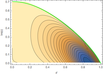
Combining graphs like those in figure 2 into a single diagram we obtain figure 4, where we use instead of on the horizontal axis. The regions of stability where are shaded and contourlines indicate constant and the constant boundary condition given by . Note that his diagram directly relates the spectral parameter of the Hill’s equation to the spectral parameter of Euler’s equation for the case of purely imaginary . Along the axis lemma 3.2 shows that . Hence the minimum occurs at corresponding to the intersection of the circles in figure 10.
The intersection of the contour with the boundary occurs at , as can also be seen in figure 2 (middle), where at . The following lemma proves this claim.
Lemma 3.3.
The derivative of with respect to at is
| (10) |
Proof.
Equation 8 is of the form with , or more generally from equation 4 where is a periodic stream function. Thus is a solution for and . Reduction of order gives a second solution . Following [MW66] the derivative is found by differentiating equation 8 with respect to where . The resulting ODE is again equation 8 but with a non-homogeneous term and can be solved using variations of constants. Defining the principal fundamental solution matrix
we apply formula (2.13) from [MW66]. Combining all of the terms into one integral, and using the facts that and that and are both periodic, formula (2.13) reduces to
| (11) |
The first integrals is elementary, and the second integral can be found using the method of residues, and hence the result follows. ∎
Remark 3.4.
We note here that equation 11 is somewhat general. All that is required for it to hold is the existence of a non-vanishing periodic solution to the Hill’s equation and formula (2.13) will reduce to equation 11.
The lemma shows that is indeed zero at , at the top left corner in figure 4. For , either real or purely imaginary, assuming that is real and negative (as shown in figure 1 right and figure 2 left), there are points of spectrum of the Hill’s equation nearby with real and positive . These satisfy some quasi-periodic boundary conditions, and hence there is some spectrum of equation 8 on the real axis. For imaginary , the derivative is negative for according to the lemma, and hence there is spectrum nearby, as can be seen in figure 4 to the right of the axis.
3.3. Complex
For complex the Hill’s equation (8) generally has a complex monodromy matrix, and hence also is complex in general. Our boundary conditions do imply, however, that needs to be real. This is a complex equation, so that we require , which is indicated by red lines in figure 5. Even though complex is irrelevant for the application to the Euler equation it is helpful to see how the spectrum with real positive (if it exists) extends to the complex -plane. In figure 5 we show a contourplot of on the complex -plane for fixed . Overlaid are the curves where in red. The reason to consider the curves of spectrum in the complex domain is that what we are looking for the special case when these curves intersect the axis of real for positive and with . In figure 5 middle such a case can be seen as the intersection of the red curve of spectrum with the positive real axis inside the shaded region where such that the boundary conditions are satisfied. This intersection means that the complex value of for which this figure is drawn is a complex eigenvalue of the Euler equation with wave number .


After this brief overview of the spectrum of the complex Hill’s equation we are now going to compute the Hill discriminant as a Fredholm determinant and using this formula construct an Evans function for the linearised Euler equation.
4. A Hill determinant
In order to prove facts about the spectrum of the linearised Euler equations via the discriminant of Hill’s equation we use Hill’s determinant. This is slightly more general than in [MW66] because here is a complex valued function, but this does not affect the computation of the Hill determinant. We need to first find the complex Fourier series of the function defined in equation 8. The Fourier series is conveniently expressed in terms of a parameter related to by
| (12) |
This is the well-known conformal Joukowski map that transforms the upper half-disk of radius 1 into the lower half plane. The upper half of the unit circle is mapped onto the unit interval , and circles of radius are mapped to ellipses with semi-major axis and semi-minor axis . The two solutions of the quadratic equation for in terms of are combined to produce a single-valued inverse map from such that for we have in the whole complex plane. The mapping is not continuous along the branch cut where the argument of the square root is negative, which occurs along the real interval . Later we will see that this interval corresponds to the continuous spectrum of the linearised Euler equation. The mapping is holomorphic on . One can check that this mapping from to implies everywhere and is attained along the branch cut. The inverse function satisfies and , and so it is sufficient to consider the positive quadrant of the -plane. Substituting into gives
| (13) |
Expanding this as geometric series in gives the Fourier series where
Because the Fourier coefficients decay exponentially and the series converges. Notice that because the factor is in the left half plane, . Expanding a solution of Hill’s equation as a Fourier series the solvability condition leads to the normalised Hill determinant. Following [MW66] in our particular case we find
Proposition 4.1.
This is Hill’s fundamental result which relates the trace of the principal fundamental solution matrix of equation 8 – the Hill discriminant – to the Hill determinant . In his original work [Hil78] Hill used these equations to determine the Floquet exponent and hence the stability of a particular solution. More generally Hill’s formula can be viewed as an equation for the spectral parameter for which quasiperiodic solutions with Floquet exponent exist. Instead in our setting the spectral parameter and the Floquet exponent are given, and we consider this as an equation for the parameter (or, equivalently ) for which such a solution exists. Here the Fourier coefficient and the higher order coefficients hidden in the definition of Hill’s determinant all depend on . This is a change of interpretation by which the original spectral parameter and hence of the linearised Euler equations becomes a parameter in Hill’s equation, while the spectral parameter in Hill’s equation is a parameter in the separated Euler’s equation.
The three cases discussed in the previous section now appear like this: 1) For real we have real and hence the Hill determinant is Hermitian and the Hill discriminant is real for real . 2) For purely imaginary we have purely imaginary , so that all are real because gives an even power of . Hence the Hill determinant is real and the Hill discriminant is real for real . 3) For complex also is complex and the Hill determinant and discriminant are complex.
The beauty of Hill’s formula is that it gives a very good approximation already for small truncation sizes. Instead of the determinant of a bi-infinite matrix denote by the determinant of the finite matrix truncated to . Thus the truncation of with (and hence matrix size ) becomes
| (16) |
The quality of approximation was important in Hill’s original application to the Moon, where he found good results already from determinants [Hil78]. Even for such severe truncation a figure similar to figure 4 computed from the approximation gives a qualitatively correct answer. This is particularly true when asking for which implies . Now factors because of discrete symmetry and expressing in terms of in the truncation of the Hill determinant gives
| (17) |
The vanishing of the last factor in the numerator is shown as a green line in figure 4. The two endpoints of the green line correspond to the roots of this factor where and hence and and hence . It should be noted that even though the result at the two endpoints is exact, for intermediate points along the boundary curve there are corrections from incorporating higher order approximations to the determinant. As already noted, along the lower boundary of figure 4 where the exact answer is obtained from Hill’s formula where since and hence . When we always have as a solution that is periodic, and hence . For the Hill discriminant this leads to , and hence . This surprising identity appears because for the three central columns of the Hill determinant are linearly dependent. It should be noted that the approximation to the Hill determinant produces the exact values at the edges and of figure 4.
In section 5 we show that when the circles in space from lemma 3.2 where are crossed in the correct direction then a pair of real eigenvalues is born. This is based on the following well-known formula, see, for example, [GK69]:
Theorem 4.2.
The derivative of a Fredholm determinant is given by
In general the computation of may of course be difficult, but in our case this turns out to be simple at .
Lemma 4.3.
The derivative of the Hill determinant with respect to at vanishes. The derivative of the Hill determinant with respect to at vanishes. In both cases it is assumed that for any integer .
Proof.
From [MW66] we have that is a Fredholm determinant. Indeed, there it is shown to be of Hill type, which means that the sum of the absolute values of the off-diagonal entries converges. A necessary condition for this is which holds for and for (so that ), and hence for all except for . The assumption that ensures that the denominators in equation 14 are non-zero. So in particular we can apply theorem 4.2 at as long as and . For this we need at . Now implies and , hence all Fourier coefficients and and are the identity. Thus the trace of needs to be computed. For either derivative the main observation is that the diagonal of is constant, and hence the diagonal of vanishes. Thus and both results follow. ∎
Note that this proof was easy because for we have for or , and hence the Fourier series of is trivial. For a more general periodic function has additional entries, and hence is more complicated, and even though the diagonal of still vanishes the result does not immediately follow.
Even though is excluded in the above proof, the Hill discriminant (and its derivatives) are of course well defined in this case as well. This is so because the Hill-determinant is multiplied by in equation 15, and for and .
5. An Evans function


Hill’s determinant allows us to compute Hill’s discriminant, which is the trace of the fundamental solution matrix of equation 8 after one period. In our setting this trace is given by . Unlike the Hill discriminant which foremost is a function of the spectral parameter of Hill’s equation, we define the Evans function as a function of the spectral parameter of the linearised Euler’s equation. Using Hill’s discriminant we can build an analytic function away from that vanishes when is in the discrete spectrum of the linearised Euler operator. Moreover, the degree of vanishing (in ) is the same as the algebraic multiplicity of 0 in the spectrum of equation 3, or equivalently, of in equation 4 with boundary conditions (5). For this reason, we call it an Evans function for equation 3, and (in a slight abuse of language) for the ‘class’ operator associated with it, which is one block of the block-diagonalised form from [Li00] of the linearised Euler equations.
Theorem 5.1.
The function
| (18) |
is an Evans function for the separated ODE (3) where is the Hill determinant depending on through the Fourier coefficients of . That is, is analytic in outside of and vanishes for values of where is in the spectrum of equation 3 with having periodic boundary conditions. The degree of vanishing of as a function of is the same as the algebraic multiplicity of as an eigenvalue of equation 3 or, equivalently of as an eigenvalue of equation 4 with boundary conditions (5).


Proof.
Equating equations (9) and (15) we see that by construction we have that when is in the discrete spectrum of the Euler equation. The rest of the proof is an application of Lemma 8.4.2 from [KP13]. In our notation, Lemma 8.4.2 from [KP13] says that the function
is entire in for fixed and it is entire in for fixed . Moreover, according to the lemma, the algebraic multiplicity of as an eigenvalue of equation 4 with boundary conditions (5) is equal to the degree of vanishing of (as a function of ). Differentiating equation 15 shows that
| (19) |
whence
because the other factor is non-vanishing,
Now suppose that . Differentiating again, we have that
and again
Repeating the procedure shows that the degree of vanishing of as a function of (and hence the degree of vanishing of on an isolated point of spectrum of the linearised Euler equations) is the same as the degree of as a function of , which by Lemma 8.4.2 from [KP13] is the same as the algebraic multiplicity of equation 4 with boundary conditions equation 5, or equivalently, the algebraic multiplicity of as a periodic eigenvalue of equation 3. ∎
For the Evans function and are parameters, and we are trying to find a (complex) such that . In figure 7 we show a contourplot of on the complex -plane for fixed . Overlaid are the curves where in red. Since the dependence of the Evans function on only appears in the single cosine term, this presentation gives the location of complex roots of the Evans function for fixed and varying .
We note that we recover the circles from lemma 3.2 from : When then and hence and which implies , such that
and thus on the circles the Evans function vanishes. A contour-plot of is shown in figure 8 left. At the minimum the value is , while at the maximum the value is 4. The critical point at the origin is degenerate. In the right part of figure 8 the eigenvalue is fixed to , and the 0-contour shows for which values of this eigenvalue occurs. Since the dependence of the Evans function on is simple the zero contour can be given explicitly by solving for such that
where the right hand side is considered as a function of for constant . The maximum of the 0-contour of occurs where . All 0-contours start at the origin because .
One property of an Evans function is that it limits to a constant for large arguments:
Lemma 5.2.
The function decays to a non-positive real constant for large
Proof.
When then and so so . Also and inserting these into equation 18 and using gives and the result follows. ∎
Notice that the limiting values of the Evans function at infinity is non-zero unless .
Lemma 5.3.
If and if , then is real for .
Proof.
When is real and then is bounded, real, and smooth on , and so has a real Fourier series, and hence must be real. All of the other terms in the expression for are real if and are. When is purely imaginary then by equation 12 is also purely imaginary. This implies that is real. Because of the particular form of the Fourier coefficients Hill’s matrix is Hermitian so that Hill’s determinant is real. The argument of in the last term may be either real of purely imaginary, but in either case the resulting value of is real. ∎
The first part of this lemma reflects the fact that if is real and then equation 8 with quasi-periodic boundary conditions represents a self adjoint operator, and so the spectrum must be real. The second part of this lemma is related to the fact that when is purely imaginary then equation 8 is PT-symmetric as discussed in Section 3.2.
The Euler equation is an infinite dimensional Hamiltonian system, and hence the spectrum must satisfy the symmetry of a Hamiltonian system. This leads to
Lemma 5.4.
Let be a root of the Evans function for fixed real . Then also , , and .
Proof.
Consider the potential in equation 8 and note that . Since is real equation 8 becomes its conjugate. Thus, if is a basis of solutions for the solution space to , then are a basis for . Thus we have that , that is, the Hill discriminant of the original equation (8), with is the complex conjugate of the original Hill discriminant (again provided ). This means that for real and . In particular, if then also . To consider what happens when we change the sign of , note that for the potential in equation 8 we have that . This means that a fundamental set of solutions (normalised to the identity) for is and , where and is a fundamental solution set to equation 8. In particular, we have that . Next we observe that Floquet’s theorem says that for any , where is a principal fundamental solution matrix to equation 8. Letting gives the result. ∎
Alternatively, note that and . The symmetry under can be seen directly in the Hill matrix. The factor is unchanged, hence is unchanged. In the Hill matrix every odd off-diagonal entry changes sign under . This can be compensated by conjugating by which leaves Hill’s determinant unchanged. Conjugating also conjugates , and . Further, since is real, in the Hill matrix every odd off-diagonal entry has the opposite sign compared to the complex conjugated matrix entry, so again provides a conjugacy to the original matrix such that . Together with the fact that , this implies as claimed.
We want to track the roots of as we move around in space. The circles where shown in figure 3 divide the parameter plane into 3 types of regions:
Definition 5.5.
- 0:
A point in region 0 is outside all circles
- I:
A point in region I is contained inside exactly one circle
- II:
A point in region II is contained inside exactly two circles
In order to show how the spectrum changes when the parameters cross from one region to another the derivatives of the Evans function are needed at the boundary circles where .
Lemma 5.6.
The derivative of the Evans function at satisfies
Proof.
Notice that implies . In lemma 4.3 we established that at and that any derivative of at vanishes. Thus computing the - or -derivative of the Evans function boils down to computing the derivative of . This gives
using at . Instead of the -derivative we start by computing the -derivate, using the same observation as before. The only difference is the final factor which comes from the chain rule, which now is
Using the result follows. ∎
The two different signs in the -derivative are related to the fact that is on the branch cut. Considering the pre-images under the Joukowski map equation 12 gives . When approaching from the inside of the unit disk in the -plane we find
so that corresponds to approaching the origin from below (for ) or from above (for ) the branch cut.
Lemma 5.7.
The directional derivative in the normal direction (from inside to out) at the circles , , where is
This is positive for and negative for .
Proof.
By Lemma 3.2 the circles are given by and the normalised gradient at the point is . Using lemma 5.6 the directional derivative of along the locus where thus is
and the result follows when putting this on the common denominator. The function changes sign when . In the limit the function approaches . ∎
The last lemma is describing the property of the contour-plot of as a function of shown in figure 8 left. On the upper arc of the circle where the Evans function is decreasing when crossing the circle towards its centre. On each of the lower arcs of the circles where the Evans function is increasing when crossing towards the respective centre. Now we show that when these circles are crossed, then a pair of pure imaginary roots appears at the origin.
Proposition 5.8.
When crossing the circle , , where from outside to in (i.e towards the centre point) and a pair of purely imaginary roots of is born out of the real axis at .
Proof.
Consider the Evans function along a curve in -parameter space that crosses the circle for in the normal direction with unit speed from the outside to the inside and define . The function defines a curve through at if the implicit function theorem holds, i.e. when the -derivative of is non-zero at . According to lemma 5.6 this holds as long as and . The derivative of the curve is given by the implicit function theorem as
using lemmas 5.6 and 5.7. As before the sign refers to the two sides of the branch cut at corresponding to . Thus two pure imaginary roots are created. ∎
The result fails at and at which are the points where circles intersect or are tangent. The propositions can be interpreted as describing a property of the contour-plot of as a function of shown in figure 8 right. In the right panel , and the contour-line is “moved” relative to the nearby circles in the direction of the inward normal of the circle. The result fails for technical reasons at because then lemma 4.3 does not hold.
In some sense the last proposition is a bifurcation result where a pair of imaginary roots bifurcates out of the origin. Note, however, that unlike in a bifurcation of roots of a polynomial where the derivative of the polynomial vanishes, here the derivative is non-zero.
Having described how a pair of purely imaginary eigenvalues (corresponding to a pair of real , hyperbolic and hence unstable) are created the last step is to make sure that they their imaginary part does not vanish. Pairs of purely imaginary eigenvalues can collide and form a complex quadruplet. In principle a complex quadruplet of eigenvalues may collide on the real -axis and form a pair of real eigenvalues (imaginary , elliptic and hence stable). The following lemma shows that this is impossible.
Lemma 5.9.
Let be real and such that there exists a quasiperiodic eigenvalue of equation 8 with a continuous eigenfunction. Then .
Proof.
If and , the potential is singular and unbounded, and so there are no positive eigenvalues with continuous eigenfunctions here. When equation 8 is a Hill’s equation with eigenvalue . We have that is a non-vanishing periodic eigenfunction on . Because it has no zeros, it is thus the eigenfunction corresponding to the largest periodic eigenvalue, and we can conclude that all of the Hill’s spectrum lies to the left of . Thus we can not have any bounded solutions for with with a positive eigenvalue either. Thus the only value of for which there exists positive quasiperiodic eigenvalues of equation 8 is . ∎
We are now ready to state the main result of this section. We have already established that there is an eigenvalue on the circles in lemma 3.2. Whenever two circles intersect the multiplicity doubles. In the following theorem we are counting all other isolated eigenvalues.
Theorem 5.10.
Consider the isolated eigenvalues as given by the zeroes of the Evans function other than . When is in region 0 there are no eigenvalues. When is in region I there is a pair of purely imaginary eigenvalues. When is in region II there are 4 eigenvalues, either two purely imaginary pairs, a single pair with multiplicity 2, or a complex quadruplet. On the boundary between region I and region II there is a pair of purely imaginary eigenvalues. For all cases half of the eigenvalues are unstable.
Proof.
We have been considering the quasiperiodic eigenvalue problem equation 8 with parameter and are looking for real positive eigenvalues with Floquet exponent . We have constructed an Evans function viewed as a function of with parameters and . By Li’s unstable disk theorem [Li00], see above theorem 2.2, there are no isolated eigenvalues in region 0. This implies that the Evans function has no zeroes when the parameters are in region 0. Consider a path of parameters from region 0 to region I that crosses the boundary circle away from . According to proposition 5.8 this creates a pair of purely imaginary roots. Hence there are 2 isolated eigenvalues in region I. Now consider a path of parameters from region I to region II. Crossing the boundary circle away from and another pair of purely imaginary roots is created. Hence there are 4 isolated eigenvalues in region II. Should the two pairs of eigenvalues coincide they are counted with multiplicity. This does in fact occur, and leads to a complex quadruplet of eigenvalues. Since we are counting with multiplicity there are always 4 isolated eigenvalues in region II. Because of lemma 5.9 it is not possible that the quadruplet of eigenvalues bifurcates onto the real axis and by Hamiltonian symmetry of the spectrum half of the eigenvalues correspond to unstable eigenvalues. ∎
To conclude this section we present some numerical results that show how the eigenvalues change in the fundamental domain in -space. Throughout we have considered as continuous parameters, such that the eigenvalues become functions of these parameters. For the case of purely imaginary curves of constant are plotted in the -plane, see figure 9. The blue curves are given in parametric form by where is determined by , or equivalently for constant purely imaginary value of . For the green curves consider for constant real part and the imaginary part as a parameter. For such given find such that . Then determine from as before and thus obtain the green curve in parametric form. The extremal values of the curve parameter are determined by . These occur at the origin in and at , respectively.
6. Back to Euler’s equations
So far we have constructed an Evans function for given parameters , determined by the wave number and the overall integer parameter vector . In the original Euler equations these are related to an integer mode number vector . When is inside the unstable disk corresponding perturbations have eigenvalues with non-zero real part. To find the unstable spectrum of the Euler equations linearised about the eigenvalues corresponding to all parameters inside the unstable disk need to be combined into a single Evans function. In the previous section it was convenient to define the Evans function to be a function of . Now putting them together we return to the original temporal spectral parameter .
Theorem 6.1.
An Evans function for the 2-dimensional Euler equations on the torus with coordinates linearised about the steady state for integers , with is given by
where .
Proof.
The wave number is an integer giving the periodicity of the perturbation in the -direction. It determines the parameters
As noted before is only defined . We choose a fundamental domain so that . 22 2 Even though the Evans function is even in , the set of points does not possess that symmetry. Thus for counting lattice points the domain is , while for considering the values of the Evans function is enough. By Li’s unstable disk theorem [Li00], see theorem 2.2, there are no unstable eigenvalues when . When we are on the boundary of the unstable disk when , and outside otherwise. When we are on the boundary of the unstable disk according to lemma 3.2 we have , and hence no eigenvalue with non-zero real part. To capture the point spectrum we can thus restrict to . Note that for large the corresponding point may be outside (or on the boundary of) the unstable disk.
When equation 3 becomes the trivial equation which has no periodic solutions other than the constant solution. So we can restrict to non-zero waver numbers with . Since in equation 18 is even in and in we can restrict to positive and instead square the Evans function. This shows that in every eigenvalue has at least multiplicity 2. So we end up with a product of over from 1 to where are functions of . Finally also is a function of , since the Evans function of the full Euler equations instead of the separated ODE is a function of .
Since the point spectrum has only finitely many elements there is no convergence problem with the product. Nevertheless, we note that using lemma 5.2 it is possible to normalise each Evans function such that its absolute value approaches 1 at infinity. ∎
Evans functions are only defined up to a non-zero multiplicative constant, so more, or fewer, terms could have been included in the product in Theorem 6.1. An obvious choice for more terms would have been to include all , while an obvious choice for fewer terms would be to remove any such that lie outside the unstable disk (see the leftmost panel of figure 10). Each of these choices would have produced an Evans function with the same roots as the one in Theorem 6.1. However, each of these choices has its own computational disadvantages. For example, choosing all requires one to normalise the Evans function for each class, in both , and , while choosing only the terms inside the unstable disk is cumbersome (and different) for different choices of , and so becomes convoluted to compute in practice. We have chosen this particular set of values of because it produces an Evans function that is readily computable, while still showcasing the importance of the unstable disk (and the lack of contribution from terms outside it).
In [LLS04, Theorem 3] it was proved that the number of non-imaginary isolated eigenvalues does not exceed twice the number of integer lattice points inside the unstable disk, not counting any lattice points on the line through (in particular not counting the origin). Numerical experiments in [Li00] and also in [DMW16] indicate that this upper bound is sharp.
For example for there are 128 lattice points in the open unstable disk of radius , not counting the origin. In this case let , and 11 times lies in region I, 26 times in region II, once (for ) on the inner boundary between region I and II, once (for ) on the boundary of the unstable disk, and once (for ) in region 0 (outside the unstable disk). On the inner boundary a pair is born at the origin, but at that moment it is not yet an unstable eigenvalue. Thus there are distinct eigenvalues with non-zero real part. The lattice points for and on and outside the unstable disk produce an Evans function factor that does not have any eigenvalues with non-zero imaginary part, in fact it is non-zero everywhere in . The 40 wave numbers are only half of the wave numbers that may have inside the unstable disk, the other half are obtained for negative . They sit in the opposite half of the circle, relative to the line through the lattice point . See [DMW16] for a few more examples of this type. Counting the number of lattice points inside a circle around the origin is a hard problem. But we don’t have to actually count this number, we just have to show that the Evans function has this number of zeroes. More precisely we have to establish that for each factor with 2 or 4 roots according to theorem 5.10 there are 2 or 4 lattice points inside the unstable disk. Combining all of the results about the Evans function we can now prove our main theorem.
Theorem 6.2.
The number of eigenvalues with non-zero real part for the 2-dimensional Euler equations on the torus linearised about the steady state with stream function for integers with is equal to twice the number of non-zero integer lattice points inside the disk of radius .
Proof.
By construction lattice points in the product that defines are inside the fundamental domain . The corresponding lattice points is which may or may not be inside the unstable disk defined by . Now consider the number of lattice points for given and arbitrary that are inside the unstable disk. We are going to show that when is in region I that number is 1, while when is in region II that number is 2. The main observation is that figure 10 and the regions it defines are translation invariant by in the direction. The unstable disk is the disk in the centre. Any point in region I in the unstable disk shifted by is again in region I, but outside the unstable disk. Thus for every in region I that point is the only lattice point in the unstable disk. For region II the situation is more interesting. Consider a lattice point (corresponding to ) inside region II in the unstable disk, say with . Shifting this lattice point by 1 to the right (corresponding to ) it is again in region II, and still inside the unstable disk. Similarly for and a shift by 1 to the left (corresponding to ). Thus for every lattice point inside region II in the unstable disk there are two lattice points inside the unstable disk.
Now according to theorem 5.10 for in region I the Evans function has two roots, while for in region II the Evans function has four roots. Combining this with the observation about lattice points just made we see that each lattice point accounts for two roots.
The exceptional case is when is on the boundary between region I and region II. As shown in theorem 5.10 this factor has two eigenvalues with non-zero real part. For this point (corresponding to ) is either outside or on the boundary of the unstable disk, and hence again the number of eigenvalues is twice the number of lattice points. Any points in region 0 are outside the unstable disk and the corresponding factor has no eigenvalues. Any points in the boundary between region 0 and region 1 are not lattice points inside the unstable disk and only have eigenvalue , and hence have no eigenvalue with non-zero real part. This exhausts all possible cases.
Finally, for every point in the fundamental domain inside the unstable disk there is another point inside the unstable disk. The Evans function is even in and , and this is why only positive are included, but each factor is squared. This doubles the number of lattice points, but also doubles the number of roots. Thus altogether the number of eigenvalues as given by roots of is equal to twice the number of non-zero lattice points inside the unstable disk. ∎
7. Summary and Discussion
We have constructed an Evans function for the linearised operator about shear flow solutions to the Euler equations of the form for relatively prime and , and have proven the sharpness of the upper bound of the number of points in the point spectrum found in [LLS04], that is the number of discrete eigenvalues of the operator is exactly twice the number of non-zero integer lattice points inside the so-called unstable disk. To compute the Evans function we separated variables in the linearisation and transformed the dispersion relation of a class into an equation of Hill’s type. We were then able to use properties of the Hill determinant to determine that points of spectrum for this class coincided with integer lattice points inside the unstable disk. Finally, we multiplied each of the relevant Evans functions for each class intersecting the unstable disk, resulting in the function given in the Evans function for the full 2+1 dimensional linear operator given in theorem 6.1.
We note that in theorems 6.1 and 6.2, we explicitly require . The reason is that otherwise we cannot conclude that there is a uni-modular transformation to our new coordinates in section 2. In particular, we are not allowed to treat . We expect that the computation can be repeated keeping the gcd as a factor so that the general statment from [LLS04] for non co-prime can be recovered.
Lastly, we note that while consider the original shear flow and its perturbations as being on the torus, we could have considered them on , and then the perturbations we have considered are those co-periodic in both and . Relaxing the conditions of co-periodicity in for example, we would get an additional parameter corresponding to the Floquet exponent of the (now only quasi-periodic) boundary conditions of equation 3, which would then filter through the calculations, effectively shifting the points of spectrum in the complex plane. Relaxing the co-periodicity condition in would do the same, only now the shifting parameter is the (now continuous) parameter . It remains to be seen which curves and/or surfaces would appear as the points of spectrum are plotted in terms of these additional parameters, as well as their relation to points in and on an “unstable disk”, which to the best of our knowledge, has yet to be defined for such boundary conditions.
8. Acknowledgements
The authors would like to thank G. Vasil for very useful discussions. RM would like to acknowledge the support of Australian Research Council under grant DP200102130. HRD and RM acknowledge support through the Australian Research Council grant DP210101102.
Appendix A Relation to Jacobi Operators
In previous papers [Li00, LLS04, DMW16] the analysis of the spectrum of the 2-dimensional Euler equations on the torus around a shear flow was done by analysing the operator in its representation in Fourier space, which after block-decomposition leads to so called classes which are represented by Jacobi operators. Let be the Fourier mode corresponding to the lattice point . Then the Jacobi operator of the class lead by is given by the difference equation
where is the spectral parameter. Since is rational in the recursion relation can be written in polynomial form as
This can be considered as coming from a Fourier transform, and to identify this we relabel the coefficients such that
Let’s start at the other end and consider a generalisation of a Hill’s equation in the form
where are periodic functions. In the simple case at hand they are just linear combinations of and . Now assuming a Fourier series solution and inserting this into the ODE and collecting coefficients in terms of gives a recursion relation for the coefficients . We obtain
Instead of derivatives we have multiplication by powers of . When multiplying the term in the Fourier series by a term of a periodic coefficient the product is . To get the recursion relation for the all exponential terms with a shifted exponent have to be relabelled to .
Since the Fourier transform turns differentiation into multiplication we see that the number of Fourier modes in the coefficients of the ODE determines the order of the DE, while the degree of the coefficients in the DE determines the number of derivatives in the ODE.
Note that the ODE can always be transformed into Hill’s form (different !)
where . However, this transformation changes the boundary conditions, which is why we need to consider quasi-periodic boundary conditions for a Hill’s equation in standard form.
Appendix B Counting Modes
We define the following map on classes. The class corresponding to the line is mapped to the point in the square given by
The coordinate is in the right range by construction, while the coordinate can be seen to be in the right class by substituting the equation for the class
into the equation for the unstable disk
and observing that points inside the unstable disk on the class have the roots of the corresponding quadratic. The discriminant of this quadratic is and so any (real) roots has .
For calculations it is easier to consider instead . This is of course the same as because of the lemma where the circles come from. The circles describe three regions in space which are described in figure 10. Now instead we consider two circles in space, one centred at and one centred at . Lemma 3.2 means that points on the unstable disk get mapped to points on the circles and in space.
We have the following three lemmata
Lemma B.1.
Suppose that and that . Then there are no integer lattice points on the line inside the unstable disk.
Lemma B.2.
Suppose that and that . Then there are two integer lattice points on the line inside the unstable disk.
Lemma B.3.
Suppose that either and that or and that . Then there is a single integer lattice point on the line inside the unstable disk.
Proof.
All three lemmas can be proved at once, by computing the intersection of the line of a class with the unstable disk in the coordinates set by and . That is we compute
where and are the intersection points of the class with the unstable disk . This gives
and so now the only thing left is to determine how many integers lie between for a fixed , but this is exactly what is described in the statement of the lemmata. That is if and then there are no integers between and and hence no integer lattice points of the class inside the unstable disk, & tc.
Expanding on this a bit, this is the number of integer points between (inclusive). This can be thought of as the number of integers such that with and . This has an upper bound of with and . The lower bound is clearly , which is achieved when , but more than that, if and then the roots of the quadratic lie in the interval , and we have exactly the statement of lemma B.1. The other two statements can be similarly arranged.
∎
References
- [Ach91] David J Acheson. Elementary fluid dynamics. Clardendon, Oxford, 1991.
- [BDM99] Carl M Bender, Gerald V Dunne, and Peter N Meisinger. Complex periodic potentials with real band spectra. Physics Letters A, 252(5):272–276, 1999.
- [Ben07] Carl M Bender. Making sense of non-hermitian hamiltonians. Reports on Progress in Physics, 70(6):947, 2007.
- [BHLL18] Blake Barker, Jeffrey Humpherys, Gregory Lyng, and Joshua Lytle. Evans function computation for the stability of travelling waves. Philosophical Transactions of the Royal Society A: Mathematical, Physical and Engineering Sciences, 376(2117):20170184, 2018.
- [BJK11] J. C. Bronski, M. A. Johnson, and T. Kapitula. An index theorem for the stability of periodic travelling waves of korteweg-de vries type. In Proc. Roy, pages 1141–1173, Soc. Edinburgh, 2011. Sect. A 141 no. 6.
- [BJK14] J. C. Bronski, M. A. Johnson, and T. Kapitula. An instability index theory for quadratic pencils and applications. Comm. Math, 327(2):521–550, 2014.
- [BNaKZ12] B. Barker, P. Noble, and L. Rodrigues adn K. Zumbrun. Stability of periodic Kuramoto-Sivashinsky waves. Appl. Math. Letters, 25(5):824–829, 2012.
- [BR05] J. Bronski and Z. Rapti. Modulational instability for nolinear Schrödinger equations with a periodic potential. Dyn. Part. Diff. Eq., 2(4):335–355, 2005.
- [CGS04] Emanuela Caliceti, Sandro Graffi, and Johannes Sjöstrand. Spectra of pt-symmetric operators and perturbation theory. Journal of Physics A: Mathematical and General, 38(1):185, 2004.
- [CM20a] W.A. Clarke and R. Marangell. A New Evans Function for Quasi-Periodic Solution of the Linearised Sine-Gordon Equation. Journal of Nonlinear Science, DOI: 10.1007/s00332-020-09655-4, 2020.
- [CM20b] W.A. Clarke and R. Marangell. Rigorous justification of the whitham modulation theory for equations of nls type. arXiv preprint arXiv:2011.09656, 2020.
- [DK06] B. Deconinck and J.N. Kutz. Computing spectra of linear operators using the Floquet-Fourier-Hill method. Journal of Computational Physics, 219:296–321, 2006.
- [DLM+20] Holger R. Dullin, Yuri Latushkin, Robert Marangell, Shibi Vasudevan, and Joachim Worthington. Instability of unidirectional flows for the 2D -Euler equations. Communnications on Pure and Applied Analysis, 19:2051–2079, 2020.
- [DLMF] NIST Digital Library of Mathematical Functions. http://dlmf.nist.gov/, Release 1.0.24 of 2019-09-15. F. W. J. Olver, A. B. Olde Daalhuis, D. W. Lozier, B. I. Schneider, R. F. Boisvert, C. W. Clark, B. R. Miller, B. V. Saunders, H. S. Cohl, and M. A. McClain, eds.
- [DMW16] Holger R Dullin, Robert Marangell, and Joachim Worthington. Instability of equilibria for the 2D Euler equations on the torus. SIAM J. Appl. Math., 76(4):1446–1470, 2016.
- [DMW19] Holger R Dullin, James D Meiss, and Joachim Worthington. Poisson structure of the three-dimensional Euler equations in Fourier space. Journal of Physics A: Mathematical and Theoretical, 52(36):365501, 2019.
- [DW18] Holger R Dullin and Joachim Worthington. Stability results for idealised shear flows on a rectangular periodic domain. J. Math. Fluid Mech., 20:473–484, 2018.
- [DW19] Holger R. Dullin and Joachim Worthington. Stability theory of the three-dimensional Euler equations. SIAM J. Appl. Math., 79(5):2168–2191, 2019.
- [Gar93] R. A. Gardner. On the structure of the spectra of periodic travelling waves. J. Math Pures Appl., 72(5):415–439, 1993.
- [GH07] T. Gallay and M. Hǎrǎguş. Stability of small periodic waves for the nonlinear Schrödinger equation. J. Differential Equations, 234:544–581, 2007.
- [GK69] Izrail Cudikovič Gohberg and M. G. Krein. Introduction to the theory of linear non-selfadjoint operators, volume 18 of Transl. Math. Monogr. Amer. Math. Soc., 1969.
- [Hil78] G. Hill. Researches in the lunar theory. Am. J. Math., 1(5):129–245, 1878.
- [HLZ17] Jeffrey Humpherys, Gregory Lyng, and Kevin Zumbrun. Multidimensional stability of large-amplitude navier–stokes shocks. Archive for Rational Mechanics and Analysis, 226(3):923–973, 2017.
- [HW79] G. H. Hardy and E. M. Wright. An Introduction to the Theory of Numbers. Clarendon Press, Oxford, 1979.
- [JLM13] C. Jones, Y. Latushkin, and R. Marangell. The Morse and Maslov indices for matrix Hill’s equations. Proceedings of Symposia in Pure Mathematics, 87:205–233, 2013.
- [JMMP13] C. K. R. T. Jones, R. Marangell, P. D. Miller, and R. G. Plaza. On the stability analysis of periodic sine-gordon traveling waves. Physica D: Nonlinear Phenomena, 251:63–74, 2013.
- [JMMP14] C. K. R. T. Jones, R. Marangell, P. D. Miller, and R. G. Plaza. Spectral and modulational stability of periodic wavetrains for the nonlinear klein-gordon equation. Journal of Differential Equations, 257(12):4632–4703, 2014.
- [KP13] Todd Kapitula and Keith Promislow. Spectral and dynamical stability of nonlinear waves. Springer, 2013.
- [LBJM19] K. P. Leisman, J. C. Bronski, M. A. Johnson, and R. Marangell. Stability of traveling wave solutions of nonlinear dispersive equations of nls type. arXiv preprint arXiv:1910.05392, 2019.
- [Li00] Y. C. Li. On 2D Euler equations. I. On the energy-Casimir stabilities and the spectra for linearized 2D Euler equations. Journal of Mathematical Physics, 41(2):728 – 758, 2000.
- [LLS04] Y. Latushkin, Y. C. Li, and M. Stanislavova. The spectrum of a linearized 2D Euler operator. Studies in Applied Mathematics, 112:259–270, 2004.
- [LV19] Y. Latushkin and S Vasudevan. Eigenvalues of the linearised 2D Euler equations via Birman-Schwinger and Lin’s operators. J. Math. Fluid Mech., 20(4):1667–1680, 2019.
- [MW66] W Magnus and S Winkler. Hill’s Equation. John Wiley, New York, 1966.
- [SGH92] FG Scholtz, HB Geyer, and FJW Hahne. Quasi-hermitian operators in quantum mechanics and the variational principle. Annals of Physics, 213(1):74–101, 1992.
- [Shi04] Kwang C Shin. On the shape of spectra for non-self-adjoint periodic schrödinger operators. Journal of Physics A: Mathematical and General, 37(34):8287, 2004.
- [SL03] R. Shvidkoy and Y. Latushkin. The essential spectrum of the linearized 2-d Euler operator is a vertical band. Contemporary Mathematics, 327:299–304, 2003.
- [TDK18] O. Trichtchenko, B. Deconinck, and R. Kollár. Stability of periodic traveling wave solutions to the kawahara equation. SIAM J. Appl. Dyn. Syst., 17(4):2761–2783, 2018.