Semiclassical fast-forward shortcuts to adiabaticity

Shortcuts to adiabaticity (STA) – strategies for attaining adiabatic outcomes in finite times – offer a set of tools for accelerating the dynamics of quantum systems, with important applications to atomic and chemical physics and quantum technologies Torrontegui et al. 2013; Masuda and Rice 2016; Guéry-Odelin et al. 2019. Considerable theoretical Demirplak and Rice 2005; Berry 2009; Masuda and Nakamura 2010; Masuda and Nakamura 2011; Ibáñez et al. 2011; Chen et al. 2011; Torrontegui et al. 2012; Ibáñez et al. 2012; del Campo 2013; Torosov et al. 2013; Vacanti et al. 2014; Torrontegui et al. 2014; Martínez-Garaot et al. 2014; Deffner et al. 2014; Takahashi 2015; Song et al. 2016; Deffner 2016; Muga et al. 2016; Martínez-Garaot et al. 2016; Mukherjee et al. 2016; Song et al. 2017; Sels and Polkovnikov 2017 and experimental Schaff et al. 2010; Schaff et al. 2011; Bason et al. 2011; Walther et al. 2012; Zhang et al. 2013; An et al. 2016; Wang et al. 2018 advances have been made in this emerging field, and have been extended to classical Hamiltonian Jarzynski 2013; Deng et al. 2013; Patra and Jarzynski 2017a; Okuyama and Takahashi 2016; Jarzynski et al. 2017; Torrontegui et al. 2017 and stochastic dynamics Tu 2014; Martínez et al. 2016; Li et al. 2017; Patra and Jarzynski 2017b; Chupeau et al. 2018.

For continuous systems with one degree of freedom, we formulate the problem of STA as follows (see Sec. V for a slightly different formulation). Consider a Hamiltonian

and let $|k(t)\rangle$ or $\phi_{k}(q,t)=\langle q|k(t)\rangle$ denote its $k$’th eigenstate, with eigenvalue $E_{k}(t)$. Here $\phi_{k}(q,t)$ is a real function and $\hat{H}_{0}(t)$ is time-dependent only in the interval $0\leq t\leq\tau$. Initializing the system in an energy eigenstate $\psi_{t\leq 0}=|n(0)\rangle$, we want it to evolve to the final eigenstate $\psi_{t\geq\tau}=|n(\tau)\rangle$. For slow driving ($\tau\rightarrow\infty$) the system naturally follows the adiabatic path $\psi_{t}=|n(t)\rangle$ at all times Griffiths 2004. But for rapid driving, additional measures – “shortcuts” – must be taken to prevent non-adiabatic transitions and guide the system to the desired final state. Here and below we suppress overall time-dependent phases when writing the state of our system.

In one STA approach, known as fast-forward (FF) driving Masuda and Nakamura 2010; Masuda and Nakamura 2011; Torrontegui et al. 2012, an auxiliary potential $U_{FF}(q,t)$ is added to $\hat{H}_{0}(t)$, where $U_{FF}$ is designed to guide the system to the final state $\psi_{\tau}=|n(\tau)\rangle$. This approach offers a promising tool for achieving the controlled acceleration of continuous quantum systems, towards desired ends such as the manipulation of Bose-Einstein condensates Torrontetui et al. 2012; Masuda 2012; Masuda et al. 2014; Masuda and Rice 2014; Masuda et al. 2018 or ions in trapping potentials Masuda and Rice 2015a; Kiely et al. 2015, or population transfer between vibrational molecular states Masuda and Rice 2015b; Masuda and Rice 2016.

Unfortunately the procedure for constructing $U_{FF}(q,t)$ generically leads to divergent behavior – “infinities” in the potential – at locations where the eigenstate $\phi_{n}(q,t)$ has nodes Martínez-Garaot et al. 2016; Patra and Jarzynski 2017b; Guéry-Odelin et al. 2019. As a result this method has been restricted to ground-state wavefunctions, which lack nodes, or else to situations in which special scale-invariant symmetries eliminate the divergences Deffner et al. 2014. Truncating divergences with finite cutoffs has proven useful when driving a system from its ground state to its first excited state (i.e. $|0(0)\rangle\rightarrow|1(\tau)\rangle$) Martínez-Garaot et al. 2016, but this strategy has not been explored for the STA problem formulated above ($|n(0)\rangle\rightarrow|n(\tau)\rangle$), and it is likely to lead to difficult-to-engineer potentials for eigenstates with many nodes.

In this paper we extend the fast-forward approach to excited states, by developing a semiclassical strategy that is free of divergences. In Sec. II we derive our main result: a semiclassically motivated recipe for constructing a divergence-free $U_{FF}(q,t)$ for excited energy eigenstates. In Sec. III we use numerical simulations to illustrate the effectiveness of this approach. We find that our fast-forward potential steers the wavefunction to the desired final eigenstate with high accuracy, with only a small amount of probability spilling out into sideband states. In Sec. IV we compare these results with corresponding classical simulations, and we develop a semiclassical theory for these sidebands. We end with a brief discussion in Sec. V. Several technical steps of our analysis are relegated to the Appendix, for clarity of presentation.

As in Refs. Jarzynski et al. 2017; Patra and Jarzynski 2017b, our starting point is a velocity field $v(q,t)$ (as yet undetermined) that vanishes for $t\notin[0,\tau]$. We then use $v(q,t)$ to define an acceleration field $a(q,t)$ from which the fast-forward potential is constructed, as follows:

Given $v(q,t)$, Eq. 2 defines $U_{FF}(q,t)$ up to an integration constant $u_{FF}(t)$, which is chosen so that $U_{FF}=0$ for $t\notin[0,\tau]$. Thus $v$, $a$ and $U_{FF}$ all vanish outside the interval $[0,\tau]$.

The task now is to design $v(q,t)$ so that $U_{FF}(q,t)$ (given by Eq. 2) generates the desired shortcut. To this end we define a function $S(q,t)$ via the relation

where the integration constant $s(t)$ is adjusted (see Appendix for details) so that $S$ obeys the Hamilton-Jacobi equation

By Eq. 3, $S(q,t)=S_{-}$ for $t\leq 0$ and $S(q,t)=S_{+}$ for $t\geq\tau$, for some constants $S_{\pm}$.

With these definitions in place we propose the ansatz

(for a given $n\geq 0$) as a solution to the time-dependent Schrödinger equation (TDSE)

Note that $\bar{\psi}_{t\leq 0}=|n(0)\rangle$ and $\bar{\psi}_{t\geq\tau}=|n(\tau)\rangle$. Substituting Eq. 5 into Eq. 6 yields (see Appendix)

where $\hat{p}=-i\hbar\partial_{q}$ and $\hat{v}(t)=v(\hat{q},t)$. Thus if we can find a function $v(q,t)$ that satisfies Eq. 7, then by construction our ansatz $\bar{\psi}$ (Eq. 5) will satisfy the TDSE, and will have the desired property of beginning and ending in the $n$’th energy eigenstate. In other words our ansatz converts the problem of constructing a potential $U_{FF}$ that satisfies Eq. 6, to that of constructing a velocity field $v$ that satisfies Eq. 7, for a given choice of $n$. We now explore strategies for accomplishing this task. In what follows, we drop the subscript $n$, and simply write $\phi(q,t)$ and $E(t)$ for the $n$’th eigenstate and eigenenergy of $\hat{H}_{0}(t)$.

Eq. 7 implies (see Appendix)

which is the continuity equation for a probability density $\phi^{2}(q,t)$ evolving under the deterministic flow $dq/dt=v(q,t)$. Thus it seems we should construct $v(q,t)$ to satisfy Eq. 8. Unfortunately the resulting velocity field generically diverges at the nodes of the eigenstate, where $\phi^{2}=0$ Patra and Jarzynski 2017b. In fact, constructing $U_{FF}$ via Eq. 8 is equivalent to previously proposed fast-forward approaches Masuda and Nakamura 2010; Masuda and Nakamura 2011; Torrontegui et al. 2012, and leads to the divergent behavior mentioned earlier. Let us therefore try a different strategy, motivated by semiclassical arguments.

In the WKB approximation, an excited eigenstate of $\hat{H}_{0}(t)$ is given by Griffiths 2004

where

Here we treat $t$ as a fixed parameter, and we consider a classical trajectory of energy $E=E(t)$ evolving under the Hamiltonian $H_{0}=p^{2}/2m+U_{0}(q,t)$. Then $q_{L}(t)$ is the left turning point of the trajectory; $\pm\bar{p}(q,t)$ are the momenta on the upper ($+$) and lower ($-$) branches of the energy shell (i.e. level set) $H_{0}(q,p,t)=E(t)$; and $\rho(q,t)$ is the position probability density sampled by the trajectory over one period of oscillation. In Eq. 10 and below, we replace the eigenenergy $E$ by its WKB approximation, determined by $\oint_{E}\bar{p}\,dq=2\pi\hbar[n+(1/2)]$.

The eigenstate probability distribution $\phi^{2}(q,t)$ oscillates with $q$ due to interference between $\phi_{+}$ and $\phi_{-}$ (Eq. 9), but after local averaging over these oscillations, $\phi^{2}(q,t)$ is semiclassically equivalent to $\rho(q,t)$ Griffiths 2004. Since the troublesome nodes in $\phi$ arise from destructive interference between $\phi_{+}$ and $\phi_{-}$, let us see what happens if we attempt to construct $v(q,t)$ to satisfy Eq. 7 separately for each term: $i\hbar\partial_{t}\phi_{\pm}=\hat{D}\phi_{\pm}$. Upon substitution and separation of real and imaginary parts (see Appendix) we obtain

To interpret these conditions, we observe that $\phi_{\pm}(q,t)$ reflects both a classical probability distribution $\rho(q,t)$ and a quantum phase $e^{\pm i(\Sigma/\hbar-\pi/4)}$. Eq. 11b is a continuity equation for $\rho(q,t)$ under the flow $dq/dt=v(q,t)$, whereas Eq. 11a implies that the phase remains constant, $d\Sigma/dt=0$, under this flow. By Eq. 9 the nodes $\{q_{\nu}(t)\}$ of $\phi(q,t)$ satisfy

thus the value of $\Sigma$ remains constant along a node $q_{\nu}(t)$, as the parameter $t$ is varied. Hence Eq. 11a implies that the field $v(q,t)$ describes the nodal “velocities” (with respect to $t$), as illustrated in Fig. 1.

Eqs. 11a and 11b are not generally satisfied by a single $v(q,t)$. We have thus replaced one condition, Eq. 8, that suffers from divergences, with a pair of conditions, Eq. 11, that cannot be simultaneously satisfied. To make further progress, we choose to satisfy Eq. 11a rather than Eq. 11b. Thus we take

and construct $U_{FF}$ using Eq. 2, in the hope that this fast-forward potential will accurately steer the wavefunction to the desired final adiabatic state. A posteriori justification of this choice will be provided later. First we describe a test of this approach, using numerical simulations of a model system evolving under the time-dependent Schrödinger equation.

We simulated a quantum particle of unit mass evolving in a potential

where $\lambda$ varies from $+16$ to $-16$ as $\lambda(t)=4\cos(\pi t/\tau)[5-\cos(2\pi t/\tau)]$, with $\tau=1.0$. The system was initialized in the state $\psi_{0}=|n(0)\rangle$, and then evolved under the time-dependent Schrödinger equation – first using the Hamiltonian $\hat{H}_{0}(t)$, then using $\hat{H}_{0}(t)+\hat{U}_{FF}(t)$, with the fast-forward potential determined by Eqs. 2 and 13 as described above.

Fig. 2 presents numerical results for $n=17$, setting $\hbar=2$. Each frame displays a histogram showing how the evolving wavefunction $\psi_{t}$ is distributed among the instantaneous eigenstates $|\phi_{k}(t)\rangle$, as quantified by the overlap $p_{k}(t)=|\langle\phi_{k}|\psi_{t}\rangle|^{2}$. Figs. 2 - 2 and 2 - 2 correspond to evolution under $\hat{H}_{0}$ and $\hat{H}_{0}+\hat{U}_{FF}$, respectively. In both cases the system evolves from $\psi_{0}=|17\rangle$ (Figs. 2, 2) to a superposition of energy eigenstates at intermediate times (Figs. 2, 2). While the system evolving under $\hat{H}_{0}(t)$ ends in a broad superposition of eigenstates, Fig. 2, the one evolving with the fast-forward shortcut reaches the final adiabatic state to a very good approximation: in Fig. 2, $p_{17}=0.91$ and $p_{16}+p_{17}+p_{18}=0.98$. Thus the potential $U_{FF}(q,t)$ constructed from Eqs. 2 and 13 achieves fast-forward driving with high accuracy. We have performed simulations using different parameter values, and have found that the potential $\hat{U}_{FF}$ consistently guides the system to a final state whose probability is concentrated in the target eigenstate $|n(\tau)\rangle$, along with a few sideband states such as $k=16,18$ in Fig. 2. (See Appendix for movies showing the evolving profile of $p_{k}(t)$ both without and with the fast forward potential.)

For evolution under $\hat{H}_{0}+\hat{U}_{FF}$, Fig. 3 shows the distributions $|\psi(q,\tau)|^{2}$ and $|\phi_{17}(q,\tau)|^{2}$. While the minima and maxima align nicely, the values of $|\psi|^{2}$ and $|\phi_{17}|^{2}$ differ visibly. This is understandable, as $v(q,t)$ was constructed to track the eigenstate’s phase $\Sigma$ (Eq. 11a) rather than its magnitude $\rho$ (Eq. 11b). The mismatch in Fig. 3 is reflected in the sidebands in Fig. 2. We now develop intuition by comparing our results with classical simulations, and we derive a semiclassical prediction for the sidebands (Eq. 15).

We first note that the potential $U_{FF}(q,t)$ determined by Eqs. 2 and 13 is identical to the one designed in Ref. Jarzynski et al. 2017 (see Eqs. 8-12 therein) for a purely classical fast-forward shortcut. This agreement reflects the Correspondence Principle (CP) and provides a measure of justification for choosing to satisfy Eq. 11a rather than Eq. 11b. Indeed, by invoking the CP we could have argued for constructing $U_{FF}(q,t)$ from Eqs. 2 and 13 directly from the classical results of Ref. Jarzynski et al. 2017, rather than by proceeding via the WKB approximation as done above. These considerations further motivate us to compare our quantum simulations with classical counterparts.

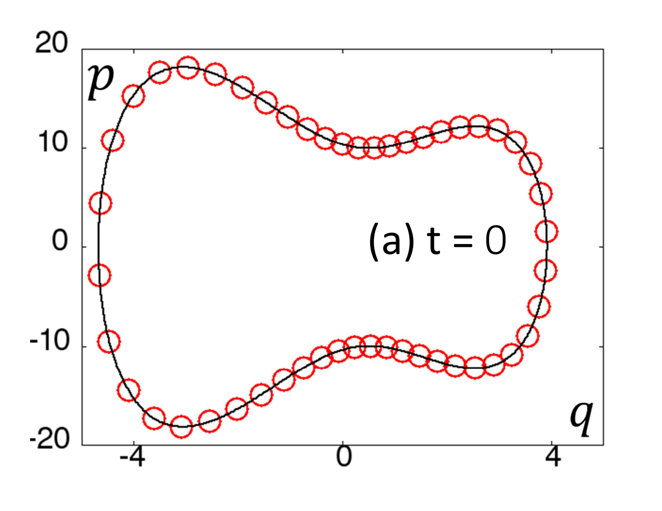
Fig. 4 depicts snapshots of 50 trajectories evolving under the classical counterpart of the Hamiltonian $\hat{H}_{0}+\hat{U}_{FF}$ used to generate Figs. 2 - 2 above, with $\tau=1.0$. Initial conditions were spaced uniformly, with respect to the angle $\theta$ of action-angle coordinates $(I,\theta)$ Goldstein 1980, over an energy shell $H_{0}(q,p,0)=53.86=E_{17}(0)$. The closed black curves depict an energy shell ${\cal E}(t)$ determined by a fixed value of the action, $I=(2\pi)^{-1}\oint\bar{p}\,dq$. We refer to ${\cal E}(t)$ as the adiabatic energy shell.

The classical action $I$ is an adiabatic invariant: for slow driving ($\tau\rightarrow\infty$), trajectories evolving under $H_{0}(q,p,t)$ cling to the adiabatic shell ${\cal E}(t)$ at all times, whereas for rapid driving ($\tau=1.0$) the trajectories evolve away from the adiabatic shell Jarzynski et al. 2017. Fig. 4 illustrates the effect of adding the fast-forward potential $U_{FF}$ when $\tau=1.0$: the trajectories at first stray “off shell”, Fig. 4, but return faithfully to the adiabatic shell at $t=\tau$, Fig. 4.

Figs. 4 - 4 are classical counterparts of Figs. 2 - 2. Observe that both final states display “imperfections”: the wavefunction in Fig. 2 does not end exactly in the eigenstate $\phi_{17}(\tau)$, and the trajectories in Fig. 4 are distributed non-uniformly over the energy shell ${\cal E}(\tau)$. These features are related. Using time-dependent WKB theory Littlejohn 1992, we obtain the following prediction for the overlap between the final wavefunction $\psi(q,\tau)$ and the eigenstate $\phi_{n+l}(q,\tau)$ (see Appendix):

where $\eta$ is the classical distribution of final conditions on the energy shell ${\cal E}(\tau)$, expressed in the angle variable $\theta$. Eq. 15 relates the sidebands in Fig. 2 to the non-uniformity of points in Fig. 4 – if the classical distribution were uniform, $\eta=1/2\pi$, the sidebands would vanish: $|\langle\phi_{n+l}|\psi\rangle|_{t=\tau}^{2}=\delta_{l0}$.

Fig. 5 compares the histogram appearing in Fig. 2 with the prediction of Eq. 15, evaluated using the trajectories in Fig 4. The evident agreement supports our semiclassical analysis, which suggests that the non-zero sidebands will persist even in the limit $\hbar\rightarrow 0$. Namely, imagine that for the same $\hat{H}_{0}(t)$ used to generate Fig. 2, we tuned the value of $\hbar$ (keeping other parameters unchanged) so that $E=53.86$ were the 1017’th, rather than 17’th, eigenenergy of $\hat{H}(0)$; and imagine we then re-ran both the quantum and classical simulations. Since the latter are unaffected by the choice of $\hbar$, we would again obtain Fig. 4, but the quantum simulations would produce a final histogram $p_{k}(\tau)$ sharply peaked at $k=1017$. Eq. 15 implies that the distribution of probability among the eigenstates $k=1014-1020$ would be the same as that observed among $k=14-20$ in Figs. 2 and 5. This implies that in the limit $\hbar\rightarrow 0$, the variance of the energy distribution associated with the non-zero sidebands tends to zero (since the energy level spacing tends to zero), consistent with a classical final state in which all trajectories end on the adiabatic energy shell (Fig. 4).

We have expanded the toolkit for accelerating quantum dynamics, by developing a method for constructing fast-forward shortcuts that are free of divergences and thereby applicable to excited states of generic kinetic-plus-potential Hamiltonians in one degree of freedom. Our approach is the semiclassical analogue of the classical method of Ref. Jarzynski et al. 2017. It will be interesting to extend our approach to systems with $d>1$ degrees of freedom. For integrable systems the existence of WKB expressions for energy eigenstates are likely to prove useful to this end, but for systems with chaotic classical dynamics the task may prove challenging. As noted elsewhere, in a number of experimentally relevant situations a separation of variables may effectively reduce a $d=3$ system to a $d=1$ system Jarzynski et al. 2017. Finally, while we have chosen to satisfy Eq. 11a in our construction of $U_{FF}(q,t)$, and have used the Correspondence Principle to justify our choice, it will be interesting to test numerically whether satisfying Eq. 11b instead would lead to a fast-forward potential capable of steering the wavefunction (approximately) to the desired final energy eigenstate.

From the start, we have assumed that the Hamiltonian $\hat{H}_{0}(t)=\hat{p}^{2}/2m+U_{0}(\hat{q},t)$ is specified for all $t\in[0,\tau]$. However, in other formulations of shortcuts to adiabaticity only initial and final Hamiltonians $\hat{H}_{0}(0)$ and $\hat{H}_{0}(\tau)$ are given, and the problem is then to construct a Hamiltonian $\hat{H}(t)$ under which an initial state $\psi(q,0)=\phi_{n}(q,0)$ evolves to a final state $\psi(q,\tau)=\phi_{n}(q,\tau)$. In this situation, we can simply choose a potential $U_{0}(q,t)$ that interpolates smoothly from $U_{0}(q,0)$ to $U_{0}(q,\tau)$ and then apply our method to obtain $U_{FF}(q,t)$. The Hamiltonian $\hat{H}(t)=\hat{p}^{2}/2m+U_{0}(\hat{q},t)+U_{FF}(\hat{q},t)$ then generates the desired evolution.

It is instructive to compare our results with those obtained for scale-invariant Hamiltonians Deffner et al. 2014, which are characterized by time-dependence of the form

Here, the parameters $f(t)$ and $\gamma(t)$ describe translations and dilations of the potential energy function. ¹¹ 1 We note in passing that a harmonic oscillator described by the potential $k(t)[q-f(t)]^{2}/2$ falls into this class, with $U_{0}(x)=x^{2}/2$ and $\gamma=k^{-1/4}$. For Hamiltonians $\hat{H}_{0}(t)$ of this form, Eqs. 8, 11a and 11b are exactly satisfied by the non-divergent velocity field $v(q,t)=\dot{f}-(\dot{\gamma}/\gamma)(q-f)$, where dots indicate derivatives with respect to time. Eq. 2 then leads to the fast-forward potential

The same potential was obtained in Ref. Deffner et al. 2014 using a trick involving canonical or unitary transformations of variables. This comparison suggests that the success of that trick may be related to the fact that Eqs. 8, 11a and 11b are solved by a single, well-behaved field $v(q,t)$, which is a particular feature of scale-invariant Hamiltonians. If this is the case then the approach of Ref. Deffner et al. 2014 might not readily generalize beyond scale-invariant Hamiltonians. This issue deserves further investigation.

Appendix

Here we provide technical details of the derivations of Eqs. 4, 7, 8, 11 and 15.

Suppose we have constructed a function $S^{\circ}(q,t)$ that satisfies $\partial_{q}S^{\circ}=mv$ (Eq. 3), without as yet adjusting the constant of integration $s(t)$. From Eqs. 2 and 3 we obtain

equivalently

hence

for some $\beta(t)$. By setting

we arrive at $S(q,t)$ that satisfies both Eqs. 3 and 4.

Substituting $\psi(q,t)$ given by Eq. 5 into the time-dependent Schrödinger equation

we separately evaluate each side using Eqs. 1 and 4 to obtain (dropping the subscript $n$)

where dots and primes denote $\partial_{t}$ and $\partial_{q}$, respectively, and $\gamma(t)=-(1/\hbar)\int_{0}^{t}E(t^{\prime})dt^{\prime}$. Setting the expressions in Eq. A6 equal to one another and using $\hat{H}_{0}\phi=E\phi$, we arrive at

Using Eq. 3 we then get

which is the desired result (Eq. 7).

Dividing both sides of Eq. 7 by $i\hbar$ and using $\hat{p}=-i\hbar\partial_{q}$, we get

Multiplying both sides by $2\phi$ we obtain

which is the continuity equation for the probability density $\phi^{2}(q,t)$.

Writing

where $A=\sqrt{\rho}$ and $\alpha=e^{-i\pi/4}$, and substituting this expression into $i\hbar\partial_{t}\phi_{+}=\hat{D}\phi_{+}$, the two sides evaluate as follows (dropping the extraneous factor $\alpha/\sqrt{2}$):

Equating these two expressions, then dividing both sides of the equation by $e^{i\Sigma/\hbar}$, and then collecting real and imaginary terms, we obtain

Dividing the first equation by $A$ and multiplying the second by $2A$, we arrive at Eq. 11. Evaluating $i\hbar\partial_{t}\phi_{-}=\hat{D}\phi_{-}$ produces identical results.

Time-dependent WKB theory Littlejohn 1992 provides a set of tools for constructing approximations to quantum wavefunctions evolving under the Schrödinger equation, from ensembles of classical trajectories obeying Hamiltonian dynamics. Applying these tools to the final wavefunction $\psi(q,\tau)$ after evolution under $\hat{H}_{0}+\hat{U}_{FF}$, we obtain (aside from an overall phase that we ignore)

where $\alpha=e^{-i\pi/4}$, $\eta_{\pm}(q,\tau)$ denote the classical probability distributions on the upper and lower branches of the energy shell $E=E_{n}(\tau)$, depicted in Fig. 4, and $\Sigma_{n}(q,t)$ is given by Eq. 10. At a given location $q$, the two terms appearing on the right side of Eq.A14 describe a right-moving and a left-moving wave train, with local momenta $\pm\bar{p}=\pm\partial_{q}\Sigma_{n}$ (since the classical trajectories all end on the adiabatic energy shell) and amplitudes $\sqrt{\eta_{\pm}}$.

We wish to take the inner product between $\psi(q,\tau)$ and the $k$’th energy eigenstate $\phi_{k}(q,\tau)$, for $k\approx n$. Time-independent WKB theory gives (see also Eq. 9)

where $\rho_{k\pm}=\rho_{k}/2$ and the subscript $k$ indicates that we are evaluating $\Sigma(q,\tau)$ and $\rho(q,\tau)$ (Eq. 10) at the energy $E=E_{k}(\tau)$. The functions $\rho_{k\pm}$ represent equal contributions to the probability distribution $\rho_{k}$ from the two branches of the energy shell.

Taking the inner product between $\phi_{k}$ and $\psi$ gives the contribution

from the upper branch, and a similar contribution $\langle\phi_{k}|\psi\rangle_{-}$ from the lower branch. (We discard cross-term contributions between the two branches, as they approximately vanish upon integrating over rapidly oscillating phases.) We now use action-angle coordinates $(\theta,I)$ to analyze these contributions. In what follows, we mostly suppress the dependence of various quantities on the constant $\tau$.

The action $I$ corresponding to energy $E$ is given by

Since the function $\Sigma$ is evaluated on a particular energy shell $E$, it can be viewed as a function of the action, $\Sigma=\Sigma(q,I)$, where $I=I(E)$. Written in this way, it is the generating function for a canonical transformation from coordinates $(q,p)$ to $(\theta,I)$ Goldstein 1980. On the upper branch of the energy shell, the angle variable $\theta\in[0,\pi]$ is given by

Defining $I_{j}\equiv I(E_{j})=\hbar[j+(1/2)]$ we obtain

The distribution $\rho_{k+}(q)$ is uniform in the angle variable, $\rho_{k+}(q)dq=d\theta/2\pi$, which allows us to perform a change of variables, from $q$ to $\theta$, in the evaluation of Eq. A16:

where

is the probability distribution on the upper branch of the energy shell, given in terms of the angle variable $\theta$.

For the lower branch of the energy shell we have $\theta=-\partial\Sigma/\partial I$ and $\rho_{k-}dq=-d\theta/2\pi$, and we obtain

with

Summing the two contributions, we get

Replacing $\int_{-\pi}^{\pi}d\theta$ with $\int_{0}^{2\pi}d\theta$ and setting $l=k-n$, we arrive at Eq. 15.

References

- Torrontegui et al. (2013) E. Torrontegui, S. Ibáñez, S. Martínez-Garaot, M. Modugno, A. del Campo, D. Guéry-Odelin, A. Ruschhaupt, X. Chen, and J. G. Muga, Adv. At. Mol. Opt. Phys. 62, 117 (2013).
- Masuda and Rice (2016) S. Masuda and S. A. Rice, Adv. Chem. Phys. 159, 51 (2016).
- Guéry-Odelin et al. (2019) D. Guéry-Odelin, A. Ruschhaupt, A. Kiely, E. Torrontegui, S. Martínez-Garaot, and J. G. Muga, Rev. Mod. Phys. 91, 045001 (2019).
- Demirplak and Rice (2005) M. Demirplak and S. A. Rice, J. Phys. Chem. B 109, 6838 (2005).
- Berry (2009) M. V. Berry, J. Phys. A: Math. Theor. 42, 365303 (2009).
- Masuda and Nakamura (2010) S. Masuda and K. Nakamura, Proc. R. Soc. A 466, 1135 (2010).
- Masuda and Nakamura (2011) S. Masuda and K. Nakamura, Phys. Rev. A 84, 043434 (2011).
- Ibáñez et al. (2011) S. Ibáñez, S. Martínez-Garaot, X. Chen, E. Torrontegui, and J. G. Muga, Phys. Rev. A 84, 023415 (2011).
- Chen et al. (2011) X. Chen, E. Torrontegui, and J. G. Muga, Phys. Rev. A 83, 062116 (2011).
- Torrontegui et al. (2012) E. Torrontegui, S. Martínez-Garaot, A. Ruschhaupt, and J. G. Muga, Phys. Rev. A 86, 013601 (2012).
- Ibáñez et al. (2012) S. Ibáñez, X. Chen, E. Torrontegui, J. G. Muga, and A. Ruschhaupt, Phys. Rev. Lett. 109, 100403 (2012).
- del Campo (2013) A. del Campo, Phys. Rev. Lett. 111, 100502 (2013).
- Torosov et al. (2013) B. T. Torosov, G. Della Valle, and S. Longhi, Phys. Rev. A 87, 052502 (2013).
- Vacanti et al. (2014) G. Vacanti, R. Fazio, S. Montangero, G. M. Palma, M. Paternostro, and V. Vedral, New J. Phys. 16, 053017 (2014).
- Torrontegui et al. (2014) E. Torrontegui, S. Martínez-Garaot, and J. G. Muga, Phys. Rev. A 89, 043408 (2014).
- Martínez-Garaot et al. (2014) S. Martínez-Garaot, E. Torrontegui, X. Chen, and J. G. Muga, Phys. Rev. A 89, 053408 (2014).
- Deffner et al. (2014) S. Deffner, C. Jarzynski, and A. del Campo, Phys. Rev. X 4, 021013 (2014).
- Takahashi (2015) K. Takahashi, Phys. Rev. A 91, 042115 (2015).
- Song et al. (2016) J. Song, Z. Zhang, Y. Xia, X. Sun, and Y. Jiang, Opt. Exp. 24, 21674 (2016).
- Deffner (2016) S. Deffner, New Journal of Physics 18, 012001 (2016).
- Muga et al. (2016) J. G. Muga, M. A. Simón, and A. Tobalina, New. J. Phys. 18, 021005 (2016).
- Martínez-Garaot et al. (2016) S. Martínez-Garaot, M. Palmero, J. G. Muga, and D. Guéry-Odelin, Phys. Rev. A 94, 063418 (2016).
- Mukherjee et al. (2016) V. Mukherjee, S. Montangero, and R. Fazio, Phys. Rev. A 93, 062108 (2016).
- Song et al. (2017) X. K. Song, F. G. Deng, L. Lamata, and J. G. Muga, Phys. Rev. A 95, 022332 (2017).
- Sels and Polkovnikov (2017) D. Sels and A. Polkovnikov, Proc. Natl. Acad. Sci. USA 114, 3909 (2017).
- Schaff et al. (2010) J.-F. Schaff, X.-L. Song, P. Vignolo, and G. Labeyrie, Phys. Rev. A 82, 033430 (2010).
- Schaff et al. (2011) J.-F. Schaff, X.-L. Song, P. Capuzzi, P. Vignolo, and G. Labeyrie, Europhys. Lett. 93, 23001 (2011).
- Bason et al. (2011) M. G. Bason, M. Viteau, N. Malossi, P. Huillery, E. Arimondo, D. Ciampini, R. Fazio, V. Giovannetti, R. Mannella, and O. Morsch, Nature Physics 8, 147 (2011).
- Walther et al. (2012) A. Walther, F. Ziesel, T. Ruster, S. T. Dawkins, K. Ott, M. Hettrich, K. Singer, F. Schmidt-Kaler, and U. Poschinger, Phys. Rev. Lett. 109, 080501 (2012).
- Zhang et al. (2013) J. Zhang, J. H. Shim, I. Niemeyer, T. Taniguchi, T. Teraji, H. Abe, S. Onoda, T. Yamamoto, T. Ohshima, J. Isoya, et al., Phys. Rev. Lett. 110, 240501 (2013).
- An et al. (2016) S. An, D. Lv, A. del Campo, and K. Kim, Nat. Comm. 7, 12999 (2016).
- Wang et al. (2018) T. Wang, Z. Zhang, L. Xiang, Z. Jia, D. P., W. Cai, Z. Gong, Z. Zong, M. Wu, J. Wu, et al., New J. Phys. 20, 065003 (2018).
- Jarzynski (2013) C. Jarzynski, Phys. Rev. A 88, 040101(R) (2013).
- Deng et al. (2013) J. Deng, Q. H. Wang, Z. Liu, P. Hänggi, and J. Gong, Phys. Rev. E 88, 062122 (2013).
- Patra and Jarzynski (2017a) A. Patra and C. Jarzynski, J. Phys. Chem. B 121, 3403 (2017a).
- Okuyama and Takahashi (2016) M. Okuyama and K. Takahashi, Phys. Rev. Lett. 117, 070401 (2016).
- Jarzynski et al. (2017) C. Jarzynski, S. Deffner, A. Patra, and Y. Subasi, Phys. Rev. E 95, 032122 (2017).
- Torrontegui et al. (2017) E. Torrontegui, I. Lizuain, S. González-Resines, A. Tobalina, A. Ruschhaupt, R. Kosloff, and J. G. Muga, Phys. Rev. A 96, 022133 (2017).
- Tu (2014) Z. C. Tu, Phys. Rev. E 89, 052148 (2014).
- Martínez et al. (2016) I. A. Martínez, A. Petrosyan, D. Guéry-Odelin, E. Trizac, and S. Ciliberto, Nat. Phys. 12, 843 (2016).
- Li et al. (2017) G. Li, H. T. Quan, and Z. C. Tu, Phys. Rev. E 96, 012144 (2017).
- Patra and Jarzynski (2017b) A. Patra and C. Jarzynski, New J. Phys. 19, 125009 (2017b).
- Chupeau et al. (2018) M. Chupeau, B. Besga, D. Guéry-Odelin, E. Trizac, A. Petrosyan, and S. Ciliberto, Phys. Rev. E 98, 010104(R) (2018).
- Griffiths (2004) D. J. Griffiths, Introduction to Quantum Mechanics (Pearson Prentice Hall, 2004), 2nd ed.
- Torrontetui et al. (2012) E. Torrontetui, X. Chen, M. Modugno, S. Schmidt, A. Ruschhaupt, and J. G. Muga, New. J. Phys. 14, 013031 (2012).
- Masuda (2012) S. Masuda, Phys. Rev. A 86, 063624 (2012).
- Masuda et al. (2014) S. Masuda, K. Nakamura, and A. del Campo, Phys. Rev. Lett. 113, 063003 (2014).
- Masuda and Rice (2014) S. Masuda and S. A. Rice, Phys. Rev. A 89, 033621 (2014).
- Masuda et al. (2018) S. Masuda, K. Nakamura, and M. Nakahara, New. J. Phys. 20, 025008 (2018).
- Masuda and Rice (2015a) S. Masuda and S. A. Rice, J. Phys. Chem. B 119, 11079 (2015a).
- Kiely et al. (2015) A. Kiely, J. P. L. McGuinness, J. G. Muga, and A. Rauschhaupt, J. Phys. B: At. Mol. Opt. Phys. 48, 075503 (2015).
- Masuda and Rice (2015b) S. Masuda and S. A. Rice, J. Phys. Chem. A 119, 3479 (2015b).
- Goldstein (1980) H. Goldstein, Classical Mechanics (Addison-Wesley, Reading, Massachusetts, 1980), 2nd ed.
- Littlejohn (1992) R. G. Littlejohn, J. Stat. Phys 68, 7 (1992).