跳到论文正文
W Papers独立论文阅读器 arXiv:2101.05756 论文正文 计算阅读时间 · 0%
引用这篇论文根据当前论文元数据生成,正式投稿前建议核对。


License: arXiv.org perpetual non-exclusive license
arXiv:2101.05756v2 [math.MG] 01 Jul 2021

The ultrametric Gromov-Wasserstein distance

Facundo Mémoli Address: Department of Mathematics and Department of Computer Science and Engineering, The Ohio State University Email address: memoli@math.osu.edu , Axel Munk Address: Institute for Mathematical Stochastics, University of Göttingen Email address: munk@math.uni-goettingen.de , Zhengchao Wan Address: Department of Mathematics, The Ohio State University Email address: wan.252@osu.edu and Christoph Weitkamp Address: Institute for Mathematical Stochastics, University of Göttingen Email address: cweitka@mathematik.uni-goettingen.de
Abstract.

In this paper, we investigate compact ultrametric measure spaces which form a subset 𝒰w\mathcal{U}^{w} of the collection of all metric measure spaces ℳw\mathcal{M}^{w}. In analogy with the notion of the ultrametric Gromov-Hausdorff distance on the collection of ultrametric spaces 𝒰\mathcal{U}, we define ultrametric versions of two metrics on 𝒰w\mathcal{U}^{w}, namely of Sturm’s Gromov-Wasserstein distance of order pp and of the Gromov-Wasserstein distance of order pp. We study the basic topological and geometric properties of these distances as well as their relation and derive for p=∞p=\infty a polynomial time algorithm for their calculation. Further, several lower bounds for both distances are derived and some of our results are generalized to the case of finite ultra-dissimilarity spaces. Finally, we study the relation between the Gromov-Wasserstein distance and its ultrametric version (as well as the relation between the corresponding lower bounds) in simulations and apply our findings for phylogenetic tree shape comparisons.

1. Introduction

Over the last decade the acquisition of ever more complex data, structures and shapes has increased dramatically. Consequently, the need to develop meaningful methods for comparing general objects has become more and more apparent. In numerous applications, e.g. in molecular biology [43, 54, 17], computer vision [61, 45] and electrical engineering [77, 55], it is important to distinguish between different objects in a pose invariant manner: two instances of the a given object in different spatial orientations are deemed to be equal. Furthermore, also the comparisons of graphs, trees, ultrametric spaces and networks, where mainly the underlying connectivity structure matters, have grown in importance [21, 29]. One possibility to compare two general objects in a pose invariant manner is to model them as metric spaces (X,dX)(X,d_{X}) and (Y,dY)(Y,d_{Y}) and regard them as elements of the collection of isometry classes of compact metric spaces denoted by ℳ\mathcal{M} (i.e. two compact metric spaces (X,dX)(X,d_{X}) and (Y,dY)(Y,d_{Y}) are in the same class if and only if they are isometric to each other which we denote by X≅YX\cong Y). It is possible to compare (X,dX)(X,d_{X}) and (Y,dY)(Y,d_{Y}) via the Gromov-Hausdorff distance [32, 41], which is a metric on ℳ\mathcal{M}. It is defined as

(1) dGH​(X,Y):=infZ,ϕ,ψdH(Z,dZ)​(ϕ⁡(X),ψ⁡(Y)),\addcontentsline{lla}{section}{\numberline q:GromovHausdorff}d_{\mathrm{GH}}(X,Y):=\inf_{Z,\phi,\psi}d^{(Z,d_{Z})}_{\mathrm{H}}(\phi(X),\psi(Y)),

where ϕ:X→Z\phi:X\to Z and ψ:Y→Z\psi:Y\to Z are isometric embeddings into a metric space (Z,dZ)(Z,d_{Z}) and dH(Z,dZ)d^{(Z,d_{Z})}_{\mathrm{H}} denotes the Hausdorff distance in ZZ. The Hausdorff distance is a metric on the collection of compact subsets of a metric space (Z,dZ)(Z,d_{Z}), which is denoted by 𝒮⁡(Z)\mathcal{S}(Z), and for A,B∈𝒮⁡(Z)A,B\in\mathcal{S}(Z) defined as follows

(2) dH(Z,dZ)​(A,B):=max⁡(supa∈Ainfb∈BdZ​(a,b),supb∈Binfa∈AdZ​(a,b)).d_{\mathrm{H}}^{(Z,d_{Z})}\left(A,B\right):=\max\left({\sup\limits_{a\in A}\operatornamewithlimits{inf\vphantom{p}}\limits_{b\in B}}d_{Z}(a,b),~\sup\limits_{b\in B}\operatornamewithlimits{inf\vphantom{p}}\limits_{a\in A}d_{Z}(a,b)\right).

While the Gromov-Hausdorff distance has been applied successfully for various shape and data analysis tasks (see e.g. [69, 12, 13, 14, 15, 20, 16, 19]), it turns out that it is generally convenient to equip the modelled objects with more structure and to model them as metric measure spaces [66, 67]. A metric measure space 𝒳=(X,dX,μX)\mathcal{X}=\left(X,d_{X},\mu_{X}\right) is a triple, where (X,dX)(X,d_{X}) denotes a metric space and μX\mu_{X} stands for a Borel probability measure on XX with full support. This additional probability measure can be thought of as signalling the importance of different regions in the modelled object. Moreover, two metric measure spaces 𝒳=(X,dX,μX)\mathcal{X}=\left(X,d_{X},\mu_{X}\right) and 𝒴=(Y,dY,μY)\mathcal{Y}=\left(Y,d_{Y},\mu_{Y}\right) are considered as isomorphic (denoted by 𝒳≅w𝒴\mathcal{X}\cong_{w}\mathcal{Y}) if and only if there exists an isometry φ:(X,dX)→(Y,dY)\varphi:(X,d_{X})\to(Y,d_{Y}) such that φ#​μX=μY\varphi_{\#}\mu_{X}=\mu_{Y}. Here, φ#\varphi_{\#} denotes the pushforward map induced by φ\varphi. From now on, ℳw\mathcal{M}^{w} denotes the collection of all (isomorphism classes of) compact metric measure spaces.

The additional structure of the metric measure spaces allows to regard the modelled objects as probability measures instead of compact sets. Hence, it is possible to substitute the Hausdorff component in Equation 1 by a relaxed notion of proximity, namely the Wasserstein distance. This distance is fundamental to a variety of mathematical developments and is also known as Kantorovich distance [47], Kantorovich-Rubinstein distance [48], Mallows distance [63] or as the Earth Mover’s distance [85]. Given a compact metric space (Z,dZ)(Z,d_{Z}), let 𝒫⁡(Z)\mathcal{P}(Z) denote the space of probability measures on ZZ and let α,β∈𝒫⁡(Z)\alpha,\beta\in\mathcal{P}(Z). Then, the Wasserstein distance of order pp, for 1≤p<∞1\leq p<\infty, between α\alpha and β\beta is defined as

(3) dW,p(Z,dZ)​(α,β):=(infμ∈𝒞⁡(α,β)∫Z×ZdZp​(x,y)​μ​(𝑑x×𝑑y))1p,\addcontentsline{lla}{section}{\numberline q:Wasserstein}d^{(Z,d_{Z})}_{\mathrm{W},p}(\alpha,\beta):=\left(\inf_{\mu\in\mathcal{C}(\alpha,\beta)}\int_{Z\times Z}d^{p}_{Z}(x,y)\,\mu(dx\times dy)\right)^{\frac{1}{p}},

and for p=∞p=\infty as

(4) dW,∞(Z,dZ)​(α,β)≔infμ∈𝒞⁡(α,β)sup(x,y)∈supp⁡(μ)dZ​(x,y),\addcontentsline{lla}{section}{\numberline q:defWassersteininfinity}d^{(Z,d_{Z})}_{\mathrm{W},\infty}(\alpha,\beta)\coloneqq\inf_{\mu\in\mathcal{C}(\alpha,\beta)}\sup_{(x,y)\in\mathrm{supp}(\mu)}d_{Z}(x,y),

where supp⁡(μ)\mathrm{supp}\left(\mu\right) stands for the support of μ\mu and 𝒞⁡(α,β)\mathcal{C}(\alpha,\beta) denotes the set of all couplings of α\alpha and β\beta, i.e., the set of all probability measures μ\mu on the product space Z×ZZ\times Z such that

μ⁡(A×Z)=α⁡(A)​ and ​μ​(Z×B)=β⁡(B)\mu(A\times Z)=\alpha(A)~\text{ and }~\mu(Z\times B)=\beta(B)

for all Borel measurable sets AA and BB of ZZ. It is worth noting that the Wasserstein distance between probability measures on the real line admits a closed form solution (see [99] and Remark 2.12).

Sturm 2006 has shown that replacing the Hausdorff distance in Equation 1 with the Wasserstein distance indeed yields a meaningful metric on ℳw\mathcal{M}^{w}. Let 𝒳=(X,dX,μX)\mathcal{X}=\left(X,d_{X},\mu_{X}\right) and 𝒴=(Y,dY,μY)\mathcal{Y}=\left(Y,d_{Y},\mu_{Y}\right) be two metric measure spaces. Then, Sturm’s Gromov-Wasserstein distance of order pp, 1≤p≤∞1\leq p\leq\infty, is defined as

(5) dGW,psturm​(𝒳,𝒴)≔infZ,ϕ,ψdW,p(Z,dZ)​(ϕ#​μX,ψ#​μY),\addcontentsline{lla}{section}{\numberline q:stdSturm}d_{\mathrm{GW},p}^{\mathrm{sturm}}(\mathcal{X},\mathcal{Y})\coloneqq\inf_{Z,\phi,\psi}d_{\mathrm{W},p}^{{(Z,d_{Z})}}(\phi_{\#}\mu_{X},\psi_{\#}\mu_{Y}),

where ϕ:X→Z\phi:X\to Z and ψ:Y→Z\psi:Y\to Z are isometric embeddings into the metric space (Z,dZ)(Z,d_{Z}).

Based on similar ideas but starting from a different representation of the Gromov-Hausdorff distance, Mémoli [66, 67] derived a computationally more tractable and topologically equivalent metric on ℳw\mathcal{M}^{w}, namely the Gromov-Wasserstein distance: For 1≤p<∞1\leq p<\infty, the pp-distortion of a coupling μ∈𝒞⁡(μX,μY)\mu\in\mathcal{C}(\mu_{X},\mu_{Y}) is defined as

(6) disp​(μ)≔(∬X×Y×X×Y|dX​(x,x′)−dY​(y,y′)|p​μ​(𝑑x×𝑑y)​μ​(d​x′×d​y′))1/p\addcontentsline{lla}{section}{\numberline q:distortion}\mathrm{dis}_{p}(\mu)\coloneqq\left(\iint_{X\times Y\times X\times Y}\big|d_{X}(x,x^{\prime})-d_{Y}(y,y^{\prime})\big|^{p}\,\mu(dx\times dy)\,\mu(dx^{\prime}\times dy^{\prime})\right)^{1/p}

and for p=∞p=\infty it is given as

dis∞​(μ)≔supx,x′∈𝒳,y,y′∈𝒴s.t.(x,y),(x′,y′)∈supp⁡(μ)|dX​(x,x′)−dY​(y,y′)|.\mathrm{dis}_{\infty}(\mu)\coloneqq\sup_{\begin{subarray}{c}x,x^{\prime}\in\mathcal{X},\,y,y^{\prime}\in\mathcal{Y}\\ s.t.\,(x,y),(x^{\prime},y^{\prime})\in\mathrm{supp}\left(\mu\right)\end{subarray}}\big|d_{X}(x,x^{\prime})-d_{Y}(y,y^{\prime})\big|.

The Gromov-Wasserstein distance of order pp, 1≤p≤∞1\leq p\leq\infty, is defined as

(7) dGW,p​(𝒳,𝒴)≔12​infμ∈𝒞⁡(μX,μY)disp​(μ).\addcontentsline{lla}{section}{\numberline q:GromovWasserstein}d_{\mathrm{GW},p}(\mathcal{X},\mathcal{Y})\coloneqq\frac{1}{2}\inf_{\mu\in\mathcal{C}(\mu_{X},\mu_{Y})}\mathrm{dis}_{p}(\mu).

It is known that in general dGW,p≤dGW,psturmd_{\mathrm{GW},p}\leq d_{\mathrm{GW},p}^{\mathrm{sturm}} and that the inequality can be strict [67]. Although both dGW,psturmd_{\mathrm{GW},p}^{\mathrm{sturm}} and dGW,pd_{\mathrm{GW},p}, 1≤p≤∞1\leq p\leq\infty, are in general NP-hard to compute [67], it is possible to efficiently approximate dGW,pd_{\mathrm{GW},p} via conditional gradient descent [67, 79]. This has led to numerous applications and extensions of this distance [4, 95, 18, 24, 87].

In many cases, since the direct computation of either of these distances can be onerous, the determination of the degree of similarity between two datasets is performed via firstly computing invariant features out of each dataset (e.g. global distance distributions [75]) and secondly by suitably comparing these features. This point of view has motivated the exploration of inverse problems arising from the study of such features [67, 93, 11, 68].

Clearly, ℳw\mathcal{M}^{w} contains various, extremely general spaces. However, in many applications it is possible to have prior knowledge about the metric measure spaces under consideration and it is often reasonable to restrict oneself to work on a specific sub-collections 𝒪w⊆ℳw\mathcal{O}^{w}\subseteq\mathcal{M}^{w}. For instance, it could be known that the metrics of the spaces considered are induced by the shortest path metric on some underlying trees and hence it is unnecessary to consider the calculation of dGW,psturmd_{\mathrm{GW},p}^{\mathrm{sturm}} and dGW,pd_{\mathrm{GW},p}, 1≤p≤∞1\leq p\leq\infty, for all of ℳw\mathcal{M}^{w}. The potential advantages of focusing on a specific sub-collection 𝒪w\mathcal{O}^{w} are twofold. On the one hand, it might be possible to use the features of 𝒪w\mathcal{O}^{w} to gain computational benefits. On the other hand, it might be possible to refine the definition dGW,psturmd_{\mathrm{GW},p}^{\mathrm{sturm}} and dGW,pd_{\mathrm{GW},p}, 1≤p≤∞1\leq p\leq\infty, to obtain more informative comparisons on 𝒪w\mathcal{O}^{w}. Naturally, it is of interest to identify and study these subclasses and the corresponding refinements. This approach has been pursued to study (variants of) the Gromov-Hausdorff distance on compact ultrametric spaces by Zarichnyi 2005 and Qiu 2009, and on compact p-metric spaces by Mémoli et al. 2019. Here, the metric space (X,dX)\left(X,d_{X}\right) is called a pp-metric space (1≤p<∞)(1\leq p<\infty), if for all x,x′,x′′∈Xx,x^{\prime},x^{\prime\prime}\in X it holds

dX​(x,x′′)≤(dX​(x,x′)p+dX​(x′,x′′)p)1/p.d_{X}(x,x^{\prime\prime})\leq\left(d_{X}(x,x^{\prime})^{p}+d_{X}(x^{\prime},x^{\prime\prime})^{p}\right)^{1/p}.

Further, the metric space (X,uX)(X,u_{X}) is called an ultrametric space, if uXu_{X} fulfills for all x,x′,x′′∈Xx,x^{\prime},x^{\prime\prime}\in X that

(8) uX​(x′,x′′)≤max⁡(uX​(x,x′),uX​(x′,x′′)).\addcontentsline{lla}{section}{\numberline q:ultratriangleineq}u_{X}(x^{\prime},x^{\prime\prime})\leq\max(u_{X}(x,x^{\prime}),u_{X}(x^{\prime},x^{\prime\prime})).

In particular, note that ultrametrics can be considered as the limiting case of pp-metrics as p→∞p\rightarrow\infty. In particular, Mémoli et al. 2019 derived a polynomial time algorithm for the calculation of the ultrametric Gromov-Hausdorff distance uGHu_{\mathrm{GH}} between two compact ultrametric spaces (X,uX)(X,u_{X}) and (Y,uY)(Y,u_{Y}) (see Section 2.2), which is defined as

(9) uGH​(X,Y):=infZ,ϕ,ψdH(Z,uZ)​(ϕ⁡(X),ψ⁡(Y)),\addcontentsline{lla}{section}{\numberline q:GromovHausdorffultrametric}u_{\mathrm{GH}}(X,Y):=\inf_{Z,\phi,\psi}d^{(Z,u_{Z})}_{\mathrm{H}}(\phi(X),\psi(Y)),

where ϕ:X→Z\phi:X\to Z and ψ:Y→Z\psi:Y\to Z are isometric embeddings into a common ultrametric space (Z,uZ)(Z,u_{Z}) and dH(Z,uZ)d^{(Z,u_{Z})}_{\mathrm{H}} denotes the Hausdorff distance on ZZ.

A further motivation to study (surrogates of) the distances dGW,psturmd_{\mathrm{GW},p}^{\mathrm{sturm}} and dGW,pd_{\mathrm{GW},p} restricted on a subset 𝒪w\mathcal{O}^{w} comes from the idea of slicing which originated as a method to efficiently estimate the Wasserstein distance dW,pℝd​(α,β)d^{\mathbb{R}^{d}}_{\mathrm{W},p}(\alpha,\beta) between probability measures α\alpha and β\beta supported in a high dimensional euclidean space ℝd\mathbb{R}^{d} [85]. The original idea is that given any line ℓ\ell in ℝd\mathbb{R}^{d} one first obtains αℓ\alpha_{\ell} and βℓ\beta_{\ell}, the respective pushforwards of α\alpha and β\beta under the orthogonal projection map πℓ:ℝd→ℓ\pi_{\ell}:\mathbb{R}^{d}\rightarrow\ell, and then one invokes the explicit formula for the Wasserstein distance for probability measures on ℝ\mathbb{R} (see Remark 2.12) to obtain a lower bound to dW,pℝd​(α,β)d^{\mathbb{R}^{d}}_{\mathrm{W},p}(\alpha,\beta) without incurring the possibly high computational cost associated to solving an optimal transportation problem. This lower bound is improved via repeated (often random) selections of the line ℓ\ell [85, 9, 53].

Recently, Le et al. 2019b pointed out that, thanks to the fact that the 11-Wasserstein distance also admits an explicit formula when the underlying metric space is a tree [28, 34, 65], one can also devise tree slicing estimates of the distance between two given probability measures by suitably projecting them onto tree-like structures. Most likely, the same strategy is successful for suitable projections on random ultrametric spaces, as on these there is also an explicit formula for the Wasserstein distance [50]. The same line of of work has also recently been explored in the Gromov-Wasserstein scenario [98, 57] and could be extended based on efficiently computable restrictions (or surrogates of) dGW,psturmd_{\mathrm{GW},p}^{\mathrm{sturm}} and dGW,pd_{\mathrm{GW},p}. Inspired by the results of Mémoli et al. 2019 on the ultrametric Gromov-Hausdorff distance and the results of Kloeckner 2015, who derived an explicit representation of the Wasserstein distance on ultrametric spaces, we study the collection of compact ultrametric measure spaces 𝒰w⊆ℳw\mathcal{U}^{w}\subseteq\mathcal{M}^{w}, where 𝒳=(X,uX,μX)∈𝒰w\mathcal{X}=\left(X,u_{X},\mu_{X}\right)\in\mathcal{U}^{w}, whenever the underlying metric space (X,uX)(X,u_{X}) is a compact ultrametric space.

In terms of applications, ultrametric spaces (and thus also ultrametric measure spaces) arise naturally in statistics as metric encodings of dendrograms [46, 19] which is a graph theoretical representations of ultrametric spaces, in the context of phylogenetic trees [90], in theoretical computer science in the probabilistic approximation of finite metric spaces [5, 35], and in physics in the context of a mean-field theory of spin glasses [71, 81].

Especially for phylogenetic trees (and dendrograms), where one tries to characterize the structure of an underlying evolutionary process or the difference between two such processes, it is important to have a meaningful method of comparison, i.e., to have a meaningful metric on 𝒰w\mathcal{U}^{w}. However, it is evident from the definition of dGW,psturmd_{\mathrm{GW},p}^{\mathrm{sturm}} and the relationship between dGW,psturmd_{\mathrm{GW},p}^{\mathrm{sturm}} and dGW,pd_{\mathrm{GW},p} (see [67]), that the ultrametric structure of 𝒳,𝒴∈𝒰w\mathcal{X},\mathcal{Y}\in\mathcal{U}^{w} is not taken into account in the computation of either dGW,psturm​(𝒳,𝒴)d_{\mathrm{GW},p}^{\mathrm{sturm}}(\mathcal{X},\mathcal{Y}) or dGW,p​(𝒳,𝒴)d_{\mathrm{GW},p}(\mathcal{X},\mathcal{Y}), 1≤p≤∞1\leq p\leq\infty. Hence, we suggest, just as for the ultrametric Gromov-Hausdorff distance, to adapt the definition of dGW,psturmd_{\mathrm{GW},p}^{\mathrm{sturm}} (see Equation 5) as well as the one of dGW,pd_{\mathrm{GW},p} (see Equation 7) and verify in the following that this makes the comparisons of ultrametric measure spaces more sensitive and leads for p=∞p=\infty to a polynomial time algorithm for the derivation of the proposed metrics.

1.1. The proposed approach

Let 𝒳=(X,uX,μX)\mathcal{X}=\left(X,u_{X},\mu_{X}\right) and 𝒴=(Y,uY,μY)\mathcal{Y}=\left(Y,u_{Y},\mu_{Y}\right) be ultrametric measure spaces. Reconsidering the definition of Sturm’s Gromov-Wasserstein distance in Equation 5, we propose to only infimize over ultrametric spaces (Z,uZ)(Z,u_{Z}) in Equation 5. Thus, we define for p∈[1,∞]p\in[1,\infty] Sturm’s ultrametric Gromov-Wasserstein distance of order pp as

(10) uGW,psturm​(𝒳,𝒴)≔infZ,ϕ,ψdW,p(Z,uZ)​(ϕ#​μX,ψ#​μY),\addcontentsline{lla}{section}{\numberline q:ultraSturm}u_{\mathrm{GW},p}^{\mathrm{sturm}}(\mathcal{X},\mathcal{Y})\coloneqq\inf_{Z,\phi,\psi}d_{\mathrm{W},p}^{{(Z,u_{Z})}}(\phi_{\#}\mu_{X},\psi_{\#}\mu_{Y}),

where ϕ:X→Z\phi:X\to Z and ψ:Y→Z\psi:Y\to Z are isometric embeddings into an ultrametric space (Z,uZ)(Z,u_{Z}).

In the subsequent sections of this paper, we will establish many theoretically appealing properties of uGW,psturmu_{\mathrm{GW},p}^{\mathrm{sturm}}. Unfortunately, we will verify that, although an explicit formula for the Wasserstein distance of order pp on ultrametric spaces exists [50], for p∈[1,∞)p\in[1,\infty) the calculation of uGW,psturmu_{\mathrm{GW},p}^{\mathrm{sturm}} yields a highly non-trivial combinatorial optimization problem (see Section 3.1.1). Therefore, we demonstrate that an adaption of the Gromov-Wasserstein distance defined in Equation 7 yields a topologically equivalent and easily approximable distance on 𝒰w\mathcal{U}^{w}. In order to define this adaption, we need to introduce some notation. For a,b≥0a,b\geq 0 and 1≤q<∞1\leq q<\infty let

Λq​(a,b)≔|aq−bq|1/q.\Lambda_{q}(a,b)\coloneqq|a^{q}-b^{q}|^{1/q}.

Further define Λ∞​(a,b)≔max⁡(a,b)\Lambda_{\infty}(a,b)\coloneqq\max(a,b) whenever a≠ba\neq b and Λ∞​(a,b)=0\Lambda_{\infty}(a,b)=0 if a=ba=b.

Now, we can rewrite dGW,pd_{\mathrm{GW},p}, 1≤p≤∞,1\leq p\leq\infty, as follows

(11) dGW,p​(𝒳,𝒴)=12​infμ∈𝒞⁡(μX,μY)(∬X×Y×X×Y(Λ1​(dX​(x,x′),dY​(y,y′)))p​μ​(𝑑x×𝑑y)​μ​(d​x′×d​y′))1/p.\addcontentsline{lla}{section}{\numberline q:p-distdelta1}d_{\mathrm{GW},p}(\mathcal{X},\mathcal{Y})=\frac{1}{2}\inf_{\mu\in\mathcal{C}(\mu_{X},\mu_{Y})}\left(\iint_{X\times Y\times X\times Y}\!\!\!\!\!\big(\Lambda_{1}(d_{X}(x,x^{\prime}),d_{Y}(y,y^{\prime}))\big)^{p}\,\mu(dx\times dy)\,\mu(dx^{\prime}\times dy^{\prime})\right)^{1/p}\!\!\!.

Considering the derivation of dGW,pd_{\mathrm{GW},p} in [67] and the results on the closely related ultrametric Gromov-Hausdorff distance studied in [70], this suggests to replace Λ1\Lambda_{1} in Equation 11 with Λ∞\Lambda_{\infty} in order to incorporate the ultrametric structures of (X,uX,μX)\left(X,u_{X},\mu_{X}\right) and (Y,uY,μY)\left(Y,u_{Y},\mu_{Y}\right) into the comparison. Hence, we define the pp-ultra-distortion of a coupling μ∈𝒞⁡(μX,μY)\mu\in\mathcal{C}(\mu_{X},\mu_{Y}) for 1≤p<∞1\leq p<\infty as

(12) dispult​(μ)≔(∬X×Y×X×Y(Λ∞​(uX​(x,x′),uY​(y,y′)))p​μ​(𝑑x×𝑑y)​μ​(d​x′×d​y′))1/p.\addcontentsline{lla}{section}{\numberline q:distortionult}\mathrm{dis}_{p}^{\mathrm{ult}}(\mu)\coloneqq\left(\iint_{X\times Y\times X\times Y}\big(\Lambda_{\infty}(u_{X}(x,x^{\prime}),u_{Y}(y,y^{\prime}))\big)^{p}\,\mu(dx\times dy)\,\mu(dx^{\prime}\times dy^{\prime})\right)^{1/p}.

and for p=∞p=\infty as

dis∞ult​(μ)≔supx,x′∈𝒳,y,y′∈𝒴s.t.(x,y),(x′,y′)∈supp⁡(μ)Λ∞​(uX​(x,x′),uY​(y,y′)).\mathrm{dis}_{\infty}^{\mathrm{ult}}(\mu)\coloneqq\sup_{\begin{subarray}{c}x,x^{\prime}\in\mathcal{X},\,y,y^{\prime}\in\mathcal{Y}\\ s.t.\,(x,y),(x^{\prime},y^{\prime})\in\mathrm{supp}\left(\mu\right)\end{subarray}}\Lambda_{\infty}(u_{X}(x,x^{\prime}),u_{Y}(y,y^{\prime})).

The ultrametric Gromov-Wasserstein distance of order p∈[1,∞]p\in[1,\infty], is given as

(13) uGW,p​(𝒳,𝒴)≔infμ∈𝒞⁡(μX,μY)dispult​(μ).u_{\mathrm{GW},p}(\mathcal{X},\mathcal{Y})\coloneqq\inf_{\mu\in\mathcal{C}(\mu_{X},\mu_{Y})}\mathrm{dis}_{p}^{\mathrm{ult}}(\mu).\addcontentsline{lla}{section}{\numberline q:defuGW}

Due to the structural similarity between dGW,pd_{\mathrm{GW},p} and uGW,pu_{\mathrm{GW},p}, we can expect (and later verify) that many properties of dGW,pd_{\mathrm{GW},p} extend to uGW,pu_{\mathrm{GW},p}. In particular, we will establish that also uGW,pu_{\mathrm{GW},p} can be approximated11 1 Here “approximation” is meant in the sense that one can write code which will locally minimize the functional. There are in general no theoretical guarantees that these algorithms will converge to a global minimum. via conditional gradient descent and admits several polynomial time computable lower bounds which are useful in applications.

It is worth mentioning that Sturm 2012 studied the family of so-called Lp,qL^{p,q}-distortion distances similar to our construction of uGW,pu_{\mathrm{GW},p}. In our language, for any p,q∈[1,∞)p,q\in[1,\infty), the Lp,qL^{p,q}-distortion distance is constructed by infimizing over the (p,q)(p,q)-distortion defined by replacing Λ∞\Lambda_{\infty} with (Λq)q(\Lambda_{q})^{q} in Equation 12. This distance shares many properties with dGW,pd_{\mathrm{GW},p}.

1.2. Overview of our results

a

We give a brief overview of our results.

Section 2. We generalize the results of Carlsson and Mémoli 2010 on the relation between ultrametric spaces and dendrograms and establish a bijection between compact ultrametric spaces and proper dendrograms (see Definition 2.1). After recalling some results on the ultrametric Gromov-Hausdorff distance (see Equation 9), we use the connection between compact ultrametric spaces and dendrograms to reformulate the explicit formula for the pp-Wasserstein distance (1≤p<∞1\leq p<\infty) on ultrametric spaces derived by Kloeckner 2015 in terms of proper dendrograms. This allows us to derive a formulation of the ∞\infty-Wasserstein distance on ultrametric spaces and to study the Wasserstein distance on compact subspaces of the ultrametric space (ℝ≥0,Λ∞)(\mathbb{R}_{\geq 0},\Lambda_{\infty}), which will be relevant when studying lower bounds of uGW,pu_{\mathrm{GW},p}, 1≤p≤∞1\leq p\leq\infty.

Section 3. We demonstrate that uGW,pu_{\mathrm{GW},p} and uGW,psturmu_{\mathrm{GW},p}^{\mathrm{sturm}}, 1≤p≤∞1\leq p\leq\infty, are pp-metrics on the collection of ultrametric measure spaces 𝒰w\mathcal{U}^{w}. We derive several alternative representations for uGW,psturmu_{\mathrm{GW},p}^{\mathrm{sturm}} and study the relation between the metrics uGW,psturmu_{\mathrm{GW},p}^{\mathrm{sturm}} and uGW,pu_{\mathrm{GW},p}. In particular, we show that, while for 1≤p<∞1\leq p<\infty it holds in general that uGW,p≤21p​uGW,psturmu_{\mathrm{GW},p}\leq 2^{\frac{1}{p}}\,u_{\mathrm{GW},p}^{\mathrm{sturm}}, both metrics coincide for p=∞p=\infty, i.e., uGW,∞=uGW,∞sturmu_{\mathrm{GW},\infty}=u_{\mathrm{GW},\infty}^{\mathrm{sturm}}. Furthermore, we show how this equality in combination with an alternative representation of uGW,∞u_{\mathrm{GW},\infty} leads to a polynomial time algorithm for the calculation of uGW,∞sturm=uGW,∞u_{\mathrm{GW},\infty}^{\mathrm{sturm}}=u_{\mathrm{GW},\infty}. Moreover, we study the topological properties of (𝒰w,uGW,psturm)(\mathcal{U}^{w},u_{\mathrm{GW},p}^{\mathrm{sturm}}) and (𝒰w,uGW,p)(\mathcal{U}^{w},u_{\mathrm{GW},p}), 1≤p≤∞1\leq p\leq\infty. Most importantly, we show that uGW,psturmu_{\mathrm{GW},p}^{\mathrm{sturm}} and uGW,pu_{\mathrm{GW},p} induce the same topology on 𝒰w\mathcal{U}^{w} which is also different from the one induced by dGW,psturm/dGW,pd_{\mathrm{GW},p}^{\mathrm{sturm}}/d_{\mathrm{GW},p}, 1≤p≤∞1\leq p\leq\infty. While we further prove that the metric spaces (𝒰w,uGW,psturm)(\mathcal{U}^{w},u_{\mathrm{GW},p}^{\mathrm{sturm}}) and (𝒰w,uGW,p)(\mathcal{U}^{w},u_{\mathrm{GW},p}), 1≤p<∞1\leq p<\infty, are neither complete nor separable metric space, we demonstrate that the ultrametric space (𝒰w,uGW,∞sturm)(\mathcal{U}^{w},u_{\mathrm{GW},\infty}^{\mathrm{sturm}}), which coincides with (𝒰w,uGW,∞)(\mathcal{U}^{w},u_{\mathrm{GW},\infty}), is complete. Finally, we establish that (𝒰w,uGW,1sturm)(\mathcal{U}^{w},u_{\mathrm{GW},1}^{\mathrm{sturm}}) is a geodesic space.

Section 4. Unfortunately, it does not seem to be possible to derive a polynomial time algorithm for the calculation of uGW,psturmu_{\mathrm{GW},p}^{\mathrm{sturm}} and uGW,pu_{\mathrm{GW},p}, 1≤p<∞1\leq p<\infty. Consequently, based on easily computable invariant features, in Section 4 we derive several polynomial time computable lower bounds for uGW,pu_{\mathrm{GW},p}, 1≤p≤∞1\leq p\leq\infty. Due to the structural similarity between dGW,pd_{\mathrm{GW},p} and uGW,pu_{\mathrm{GW},p}, these are in a certain sense analogue to those derived in [66, 67] for dGW,pd_{\mathrm{GW},p}. Among other things, we show that

(14) uGW,p​(𝒳,𝒴)≥𝐒𝐋𝐁pult​(𝒳,𝒴)≔infγ∈𝒞⁡(μX⊗μX,μY⊗μY)‖Λ∞​(uX,uY)‖Lp​(γ).u_{\mathrm{GW},p}(\mathcal{X},\mathcal{Y})\geq\mathbf{SLB}_{p}^{\mathrm{ult}}(\mathcal{X},\mathcal{Y})\coloneqq\inf_{\gamma\in\mathcal{C}(\mu_{X}\otimes\mu_{X},\mu_{Y}\otimes\mu_{Y})}\left\lVert\Lambda_{\infty}(u_{X},u_{Y})\right\rVert_{L^{p}(\gamma)}.

We verify that the lower bound 𝐒𝐋𝐁pult\mathbf{SLB}_{p}^{\mathrm{ult}} can be reformulated in terms of the Wasserstein distance on the ultrametric space (ℝ≥0,Λ∞)(\mathbb{R}_{\geq 0},\Lambda_{\infty}) (we derive an explicit formula for dW,p(ℝ≥0,Λ∞)d_{\mathrm{W},p}^{(\mathbb{R}_{\geq 0},\Lambda_{\infty})} in Section 2.3). This allows us to efficiently calculate 𝐒𝐋𝐁pult​(𝒳,𝒴)\mathbf{SLB}_{p}^{\mathrm{ult}}(\mathcal{X},\mathcal{Y}) in O⁡((m∨n)2)O((m\vee n)^{2}), where mm stands for the cardinality of XX and nn for the one of YY.

Section 5. As the ultrametric space assumption is somewhat restrictive (especially in the context of phylogenetic trees, see [90]), we prove in Section 5 that the results on uGW,pu_{\mathrm{GW},p} can be extended to the more general ultra-dissimilarity spaces (see Definition 5.1). In particular, we prove that uGW,pu_{\mathrm{GW},p}, 1≤p≤∞1\leq p\leq\infty, is a metric on the isomorphism classes of ultra-dissimilarity spaces (see Definition 5.5).

Section 6. We illustrate the behaviour and relation between uGW,1u_{\mathrm{GW},1} (which can be approximated via conditional gradient descent) and 𝐒𝐋𝐁1ult\mathbf{SLB}_{1}^{\mathrm{ult}} in a set of illustrative examples. Additionally, we carefully illustrate the differences between uGW,1u_{\mathrm{GW},1} and 𝐒𝐋𝐁1ult\mathbf{SLB}_{1}^{\mathrm{ult}}, and dGW,1d_{\mathrm{GW},1} and 𝐒𝐋𝐁1\mathbf{SLB}_{1} (see Section 4 for a definition), respectively.

Section 7. Finally, we apply our ideas to phylogenetic tree shape comparison. To this end, we compare two sets of phylogenetic tree shapes based on the HA protein sequences from human influenza collected in different regions with the lower bound 𝐒𝐋𝐁1ult\mathbf{SLB}_{1}^{\mathrm{ult}}. In particular, we contrast our results in both settings to the ones obtained with the tree shape metric introduced in Equation (4) of Colijn and Plazzotta 2018.

1.3. Related work

In order to better contextualize our contribution, we now describe related work, both in applied and computational geometry, and in phylogenetics (where notions of distance between trees have arisen naturally).

Metrics between trees: the phylogenetics perspective

In phylogenetics, where one chief objective is to infer the evolutionary relationship between species via methods that evaluate observable traits, such as DNA sequences, the need to be able to measure dissimilarity between different trees arises from the fact that the process of reconstruction of a phylogenetic tree may depend on the set of genes being considered. At the same time, even for the same set of genes, different reconstruction methods could be applied which would result in different trees. As such, this has led to the development of many different metrics for measuring distance between phylogenetic trees. Examples include the Robinson-Foulds metric [84], the subtree-prune and regraft distance [42], and the nearest-neighbor interchange distance [83].

As pointed out in [76], many of these distances tend to quantify differences between tree topologies and often do not take into account edge lengths. A certain phylogenetic tree metric space which encodes for edge lengths was proposed in [6] and studied algorithmically in [76]. This tree space assumes that the all trees have the same set of taxa. An extension to the case of trees over different underlying sets is given in [40]. Lafond et al. 2019 considered one type of metrics on possibly muiltilabeled phylogenetic trees with a fixed number of leafs. As the authors pointed out, a multilabeled phylogenetic tree in which no leafs are repeated is just a standard phylogenetic tree, whereas a multilabeled phylogenetic tree in which all labels are equal defines a tree shape. The authors then proceeded to study the computational complexity associated to generalizations of some of the usual metrics for phylogenetic trees (such as the Robinson-Foulds distance) to the multilabeled case. Colijn and Plazzotta 2018 studied a metric between (binary) phylogenetic tree shapes based on a bottom to top enumeration of specific connectivity structures. The authors applied their metric to compare evolutionary trees based on the HA protein sequences from human influenza collected in different regions.

Metrics between trees: the applied geometry perspective

From a different perspective, ideas from applied geometry and applied and computational topology have been applied to the comparison of tree shapes in applications in probability, clustering and applied and computational topology.

Metric trees are also considered in probability theory in the study of models for random trees together with the need to quantify their distance; Evans 2007 described some variants of the Gromov-Hausdorff distance between metric trees. See also [39] for the case of metric measure space representations of trees and a certain Gromov-Prokhorov type of metric on the collection thereof.

Trees, in the form of dendrograms, are abundant in the realm of hierarhical clustering methods. In their study of the stability of hierarchical clustering methods, Carlsson and Mémoli 2010 utilized the Gromov-Hausdorff distance between the ultrametric representation of dendrograms. Schmiedl 2017 proved that computing the Gromov-Hausdorff distance between tree metric spaces is NP-hard. Liebscher 2018 suggested some variants of the Gromov-Hausdorff distance which are applicable in the context of phylogenetic trees. As mentioned before, Zarichnyi 2005 introduced the ultrametric Gromov-Hausdorff distance uGHu_{\mathrm{GH}} between compact ultrametric spaces (a special type of tree metric spaces). Certain theoretical properties such as precompactness of uGHu_{\mathrm{GH}} has been studied in [80]. In contrast with the NP-hardness of computing dGHd_{\mathrm{GH}}, Mémoli et al. 2019 devised an polynomial time algorithm for computing uGHu_{\mathrm{GH}}.

In computational topology merge trees arise through the study of the sublevel sets of a given function [1, 82] with the goal of shape simplification. Morozov et al. 2013 developed the notion of interleaving distance between merge trees which is related to the Gromov-Hausdorff distance between trees through bi-Lipschitz bounds. In [2], exploiting the connection between the interleaving distance and the Gromov-Hausdorff between metric trees, the authors approached the computation of the Gromov-Hausdorff distance between metric trees in general and provide certain approximation algorithms. Touli and Wang 2018 devised fixed-parameter tractable (FPT) algorithms for computing the interleaving distance between metric trees. One can imply from their methods an FPT algorithm to compute a 2-approximation of the Gromov-Hausdorff distance between ultrametric spaces. Mémoli et al. 2019 devised an FPT algorithm for computing the exact value of the Gromov-Hausdorff distances between ultrametric spaces.

2. Preliminaries

In this section we briefly summarize the basic notions and concepts required throughout the paper.

2.1. Ultrametric spaces and dendrograms

We begin by describing compact ultrametric spaces in terms of proper dendrograms. To this end, we introduce some definitions and some notation. Given a set XX, a partition of XX is a set PX={Xi}i∈IP_{X}=\{X_{i}\}_{i\in I} where II is any index set, ∅≠Xi⊆X\emptyset\neq X_{i}\subseteq X, Xi∩Xj=∅X_{i}\cap X_{j}=\emptyset for all i≠j∈Ii\neq j\in I and ⋃i∈IXi=X\bigcup_{i\in I}X_{i}=X. We call each element XiX_{i} a block of the given partition PXP_{X} and denote by 𝐏𝐚𝐫𝐭⁡(X)\mathbf{Part}(X) the collection of all partitions of XX. For two partitions PXP_{X} and PX′P^{\prime}_{X} we say that PXP_{X} is finer than PX′P^{\prime}_{X}, if for every block Xi∈PXX_{i}\in P_{X} there exists a block Xj′∈PX′X^{\prime}_{j}\in P^{\prime}_{X} such that Xi⊆Xj′X_{i}\subseteq X^{\prime}_{j}.

Definition 2.1 (Proper dendrogram).

Given a set XX (not necessarily finite), a proper dendrogram θX:[0,∞)→𝐏𝐚𝐫𝐭⁡(X)\theta_{X}:[0,\infty)\rightarrow\mathbf{Part}(X) is a map satisfying the following conditions:

  1. (1)

    θX​(s)\theta_{X}(s) is finer than θX​(t)\theta_{X}(t) for any 0≤s<t<∞0\leq s<t<\infty;

  2. (2)

    θX​(0)\theta_{X}(0) is the finest partition consisting only singleton sets;

  3. (3)

    There exists T>0T>0 such that for any t≥Tt\geq T, θX​(t)={X}\theta_{X}(t)=\{X\} is the trivial partition;

  4. (4)

    For each t>0t>0, there exists ε>0\varepsilon>0 such that θX​(t)=θX​(t′)\theta_{X}(t)=\theta_{X}(t^{\prime}) for all t′∈[t,t+ε]t^{\prime}\in[t,t+\varepsilon].

  5. (5)

    For any distinct points x,x′∈Xx,x^{\prime}\in X, there exists Tx​x′>0T_{xx^{\prime}}>0 such that xx and x′x^{\prime} belong to different blocks in θX​(Tx​x′)\theta_{X}(T_{xx^{\prime}}).

  6. (6)

    For each t>0t>0, θX​(t)\theta_{X}(t) consists of only finitely many blocks.

  7. (7)

    Let {tn}n∈ℕ\{t_{n}\}_{n\in\mathbb{N}} be a decreasing sequence such that limn→∞tn=0\lim_{n\rightarrow\infty}t_{n}=0 and let Xn∈θX​(tn)X_{n}\in\theta_{X}(t_{n}). If for any 1≤n<m1\leq n<m, Xm⊆XnX_{m}\subseteq X_{n}, then ⋂n∈ℕXn≠∅\bigcap_{n\in\mathbb{N}}X_{n}\neq\emptyset.

When XX is finite, a function θX:[0,∞)→𝐏𝐚𝐫𝐭⁡(X)\theta_{X}:[0,\infty)\rightarrow\mathbf{Part}(X) satifying conditions (1) to (4) will satisfy conditions (5), (6) and (7) automatically, and thus a proper dendrogram reduces to the usual dendrogram (see [19, Sec. 3.1] for a formal definition). Let θX\theta_{X} be a proper dendrogram over a set XX. For any x∈Xx\in X and t≥0t\geq 0, we denote by [x]tX[x]_{t}^{X} the block in θ⁡(t)\theta(t) that contains x∈Xx\in X and abbreviate [x]tX[x]_{t}^{X} to [x]t[x]_{t} when the underlying set XX is clear from the context. Similar to [19], who considered the relation between finite ultrametric spaces and dendrograms, we will prove that there is a bijection between compact ultrametric spaces and proper dendrograms. In particular, one can show that the subsequent theorem generalizes [19, Theorem 9]. Since its proof depends on several concepts not yet introduced, we postpone it to Section A.1.1.

Theorem 2.2.

Given a set XX, denote by 𝒰⁡(X)\mathcal{U}(X) the collection of all compact ultrametrics on XX and 𝒟⁡(X)\mathcal{D}(X) the collection of all proper dendrograms over XX. For any θ∈𝒟⁡(X)\theta\in\mathcal{D}(X), consider uθu_{\theta} defined as follows:

∀x,x′∈X,uθ(x,x′)≔inf{t≥0|x,x′ belong to the same block of θ(t)}.\forall x,x^{\prime}\in X,\,\,\,u_{\theta}(x,x^{\prime})\coloneqq\inf\{t\geq 0\,|\,x,x^{\prime}\text{ belong to the same block of }\theta(t)\}.

Then, uθ∈𝒰⁡(X)u_{\theta}\in\mathcal{U}(X) and the map ΔX:𝒟⁡(X)→𝒰⁡(X)\Delta_{X}:\mathcal{D}(X)\rightarrow\mathcal{U}(X) sending θ\theta to uθu_{\theta} is a bijection.

Remark 2.3.

From now on, we denote by θX\theta_{X} the proper dendrogram corresponding to a given compact ultrametric uXu_{X} on XX under the bijection given above. Note that a block [x]t[x]_{t} in θX​(t)\theta_{X}(t) is actually the closed ball Bt​(x)B_{t}(x) in XX centered at xx with radius tt. So for each t≥0t\geq 0, θX​(t)\theta_{X}(t) partitions XX into a union of several closed balls in XX with respect to uXu_{X}.

2.2. The ultrametric Gromov-Hausdorff distance

Both dGW,psturmd_{\mathrm{GW},p}^{\mathrm{sturm}} and dGW,pd_{\mathrm{GW},p}, 1≤p≤∞1\leq p\leq\infty, are by construction closely related to the Gromov-Hausdorff distance. In a recent paper, Mémoli et al. 2019 studied an ultrametric version of this distance, namely the ultrametric Gromov-Hausdorff distance (denoted as uGHu_{\mathrm{GH}}). Since we will demonstrate several connections between uGW,psturmu_{\mathrm{GW},p}^{\mathrm{sturm}}, uGW,pu_{\mathrm{GW},p}, 1≤p≤∞1\leq p\leq\infty, and this distance, we briefly summarize some of the results in [70]. We start by recalling the formal definition of uGHu_{\mathrm{GH}}.

Definition 2.4.

Let (X,uX)(X,u_{X}) and (Y,uY)(Y,u_{Y}) be two compact ultrametric spaces. Then, the ultrametric Gromov-Hausdorff between XX and YY is defined as

uGH​(X,Y)=infZ,ϕ,ψdHZ​(ϕ⁡(X),ψ⁡(Y)),u_{\mathrm{GH}}(X,Y)=\inf_{Z,\phi,\psi}d^{Z}_{\mathrm{H}}\left(\phi(X),\psi(Y)\right),

where ϕ:X→Z\phi:X\to Z and ψ:Y→Z\psi:Y\to Z are isometric embeddings (distance preserving transformations) into the ultrametric space (Z,uZ)(Z,u_{Z}).

Zarichnyi 2005 has shown that uGHu_{\mathrm{GH}} is an ultrametric on the isometry classes of compact ultrametric spaces, which are denoted by 𝒰\mathcal{U}, and Mémoli et al. 2019 identified a structural theorem (cf. Theorem 2.5) that gives rise to a polynomial time algorithm for the calculation of uGHu_{\mathrm{GH}}. More precisely, it was proven in [70] that uGHu_{\mathrm{GH}} can be calculated via so-called quotient ultrametric spaces, which we define next. Let (X,uX)(X,u_{X}) be an ultrametric space and let t≥0t\geq 0. We define an equivalence relation ∼t\sim_{t} on XX as follows: x∼tx′x\sim_{t}x^{\prime} if and only if uX​(x,x′)≤tu_{X}(x,x^{\prime})\leq t. We denote by [x]tX[x]^{X}_{t} (resp. [x]t[x]_{t}) the equivalence class of xx under ∼t\sim_{t} and by XtX_{t} the set of all such equivalence classes. In fact, [x]tX={x′∈X|u⁡(x,x′)≤t}[x]_{t}^{X}=\{x^{\prime}\in X|\,u(x,x^{\prime})\leq t\} is exactly the closed ball centered at xx with radius tt and corresponds to a block in the corresponding proper dendrogram θX​(t)\theta_{X}(t) (see Remark 2.3). Thus, one can think of XtX_{t} as a “set representation” of θX​(t)\theta_{X}(t). We define an ultrametric uXtu_{X_{t}} on XtX_{t} as follows:

uXt​([x]t,[x′]t)≔{uX​(x,x′),[x]t≠[x′]t0,[x]t=[x′]t.u_{X_{t}}([x]_{t},[x^{\prime}]_{t})\coloneqq\begin{cases}u_{X}(x,x^{\prime}),&[x]_{t}\neq[x^{\prime}]_{t}\\ 0,&[x]_{t}=[x^{\prime}]_{t}.\end{cases}

Then, (Xt,uXt)(X_{t},u_{X_{t}}) is an ultrametric space and we call (Xt,uXt)(X_{t},u_{X_{t}}) the quotient of (X,uX)(X,u_{X}) at level tt (see Figure 1 for an illustration). It is straightforward to prove that the quotient of a compact ultrametric space at level t>0t>0 is a finite ultrametric space (cf. [102, Lemma 2.3]). Furthermore, the quotient spaces characterize uGHu_{\mathrm{GH}} as follows.

Theorem 2.5 (Structural theorem for uGHu_{\mathrm{GH}}, [70, Theorem 5.7]).

Let (X,uX)(X,u_{X}) and (Y,uY)(Y,u_{Y}) be two compact ultrametric spaces. Then,

uGH​(X,Y)=inf{t≥0|Xt≅Yt}.u_{\mathrm{GH}}(X,Y)=\inf\left\{t\geq 0\,|\,X_{t}\cong Y_{t}\right\}.
Refer to caption
Figure 1. Metric quotient: An ultrametric space (black) and its quotient at level tt (red).
Remark 2.6.

Let (X,uX)(X,u_{X}) and (Y,uY)(Y,u_{Y}) denote two finite ultrametric spaces and let t≥0t\geq 0. The quotient spaces XtX_{t} and YtY_{t} can be considered as vertex weighted, rooted trees [70]. Hence, it is possible to check whether Xt≅YtX_{t}\cong Y_{t} in polynomial time [3]. Consequently, Theorem 2.5 induces a simple, polynomial time algorithm to calculate uGHu_{\mathrm{GH}} between two finite ultrametric spaces.

2.3. Wasserstein distance on ultrametric spaces

Kloeckner 2015 uses the representation of ultrametric spaces as so called synchronized rooted trees to derive an explicit formula for the Wasserstein distance on ultrametric spaces. By the constructions of the dendrograms and of the synchronized rooted trees (see Section A.2.1), it is immediately clear how to reformulate the results of Kloeckner 2015 on compact ultrametric spaces in terms of proper dendrograms. To this end, we need to introduce some notation. For a compact ultrametric space XX, let θX\theta_{X} be the associated proper dendrogram and let V(X)≔⋃t>0θX(t)={[x]t|x∈X,t>0}V(X)\coloneqq\bigcup_{t>0}\theta_{X}(t)=\{[x]_{t}|\,x\in X,t>0\}. It can be shown that V⁡(X)V(X) is the collection of all closed balls in XX except for singletons {x}\{x\} such that xx is a cluster point22 2 A cluster point xx in a topological space XX is such that any neighborhood of xx contains countably many points in XX. (see Lemma A.8). For B∈V⁡(X)B\in V(X), we denote by B∗B^{*} the smallest (under inclusion) element in V⁡(X)V(X) such that B⫋B∗B\subsetneqq B^{*} (for the existence and uniqueness of B∗B^{*} see Lemma A.1).

Theorem 2.7 (The Wasserstein distance on ultrametric spaces, [50, Theorem 3.1]).

Let (X,uX)(X,u_{X}) be a compact ultrametric space. For all α,β∈𝒫⁡(X)\alpha,\beta\in\mathcal{P}(X) and 1≤p<∞1\leq p<\infty, we have

(15) (dW,pX)p​(α,β)=2−1​∑B∈V⁡(X)\{X}(diam​(B∗)p−diam​(B)p)​|α⁡(B)−β⁡(B)|.\left(d_{\mathrm{W},p}^{X}\right)^{p}(\alpha,\beta)=2^{-1}\sum_{B\in V(X)\backslash\{X\}}\left(\mathrm{diam}\left(B^{*}\right)^{p}-\mathrm{diam}\left(B\right)^{p}\right)\left|\alpha(B)-\beta(B)\right|.

While Theorem 2.7 is only valid for p<∞p<\infty, it can be extended to the case p=∞p=\infty.

Lemma 2.8.

Let XX be a compact ultrametric space. Then, for any α,β∈P⁡(X)\alpha,\beta\in P(X), we have

(16) dW,∞X​(α,β)=maxB∈V⁡(X)\{X}​ and ​α​(B)≠β⁡(B)⁡diam⁡(B∗).\addcontentsline{lla}{section}{\numberline q:ultraWassersteininfinity}d_{\mathrm{W},\infty}^{X}(\alpha,\beta)=\max_{B\in V(X)\backslash\{X\}\text{ and }\alpha(B)\neq\beta(B)}\mathrm{diam}\left(B^{*}\right).

The proof of Lemma 2.8 is technical and we postpone it to Section A.1.2.

2.3.1. Wasserstein distance on (ℝ≥0,Λ∞)(\mathbb{R}_{\geq 0},\Lambda_{\infty})

The non-negative half real line ℝ≥0\mathbb{R}_{\geq 0} endowed with Λ∞\Lambda_{\infty} turns out to be an ultrametric space (cf. [70, Remark 1.14]). Finite subspaces of (ℝ≥0,Λ∞)(\mathbb{R}_{\geq 0},\Lambda_{\infty}) are of particular interest in this paper. These spaces possess a particular structure (see Figure 2) and the computation of the Wasserstein distance on them can be further simplified.

Refer to caption
Figure 2. Illustration of (ℝ≥0,Λ∞)(\mathbb{R}_{\geq 0},\Lambda_{\infty}): This is the dendrogram for a subspace of (ℝ≥0,Λ∞)(\mathbb{R}_{\geq 0},\Lambda_{\infty}) consisting of 5 arbitrary distinct points of ℝ+\mathbb{R}_{+}.
Theorem 2.9 (dW,p(ℝ≥0,Λ∞)d^{(\mathbb{R}_{\geq 0},\Lambda_{\infty})}_{\mathrm{W},p} between finitely supported measures).

Suppose α,β\alpha,\beta are two probability measures supported on a finite subset {x0,…,xn}\{x_{0},\dots,x_{n}\} of (ℝ≥0,Λ∞)(\mathbb{R}_{\geq 0},\Lambda_{\infty}) such that 0≤x0<x1<⋯<xn0\leq x_{0}<x_{1}<\dots<x_{n}. Denote αi≔α⁡({xi})\alpha_{i}\coloneqq\alpha(\{x_{i}\}) and βi≔β⁡({xi})\beta_{i}\coloneqq\beta(\{x_{i}\}). Then, we have for p∈[1,∞)p\in[1,\infty) that

(17) dW,p(ℝ≥0,Λ∞)​(α,β)=2−1p​(∑i=0n−1|∑j=0i(αj−βj)|⋅|xi+1p−xip|+∑i=0n|αi−βi|⋅xip)1p.\addcontentsline{lla}{section}{\numberline q:dpfinite}d^{(\mathbb{R}_{\geq 0},\Lambda_{\infty})}_{\mathrm{W},p}(\alpha,\beta)=2^{-\frac{1}{p}}\left(\sum_{i=0}^{n-1}\left|\sum_{j=0}^{i}(\alpha_{j}-\beta_{j})\right|\cdot|x_{i+1}^{p}-x_{i}^{p}|+\sum_{i=0}^{n}|\alpha_{i}-\beta_{i}|\cdot x_{i}^{p}\right)^{\frac{1}{p}}.

Let FαF_{\alpha} and FβF_{\beta} denote the cumulative distribution functions of α\alpha and β\beta, respectively. Then, for the case p=∞p=\infty we obtain

dW,∞(ℝ≥0,Λ∞)​(α,β)=max⁡(max0≤i≤n−1,Fα​(xi)≠Fβ​(xi)⁡xi+1,max0≤i≤n,αi≠βi⁡xi).d_{\mathrm{W},\infty}^{(\mathbb{R}_{\geq 0},\Lambda_{\infty})}(\alpha,\beta)=\max\left(\max_{0\leq i\leq n-1,F_{\alpha}(x_{i})\neq F_{\beta}(x_{i})}x_{i+1},\max_{0\leq i\leq n,\alpha_{i}\neq\beta_{i}}x_{i}\right).
Proof.

Clearly, V(X)={{x0,x1,…,xi}|i=1,…,n}∪{{xi}|i=1,…,n}V(X)=\{\{x_{0},x_{1},\ldots,x_{i}\}|\,i=1,\ldots,n\}\cup\{\{x_{i}\}|\,i=1,\ldots,n\} (recall that each set corresponds to a closed ball). Thus, we conclude the proof by applying Theorem 2.7 and Lemma 2.8. ∎

Remark 2.10 (The case p=1p=1).

Note that when p=1p=1, for any finitely supported probability measures α,β∈𝒫⁡(ℝ≥0)\alpha,\beta\in\mathcal{P}(\mathbb{R}_{\geq 0}),

dW,1(ℝ≥0,Λ∞)​(α,β)=12​(dW,1(ℝ,Λ1)​(α,β)+∫ℝx​|α−β|​(𝑑x)).d_{\mathrm{W},1}^{(\mathbb{R}_{\geq 0},\Lambda_{\infty})}(\alpha,\beta)=\frac{1}{2}\left(d_{\mathrm{W},1}^{(\mathbb{R},\Lambda_{1})}(\alpha,\beta)+\int_{\mathbb{R}}x\,|\alpha-\beta|(dx)\right).

The formula indicates that the 11-Wasserstein distance on (ℝ≥0,Λ∞)(\mathbb{R}_{\geq 0},\Lambda_{\infty}) is the average of the usual 11-Wasserstein distance on (ℝ≥0,Λ1)(\mathbb{R}_{\geq 0},\Lambda_{1}) and a “weighted total variation distance”. The weighted total variation like distance term is sensitive to difference of supports. For example, let α=δx1\alpha=\delta_{x_{1}} and β=δx2\beta=\delta_{x_{2}}, then ∫ℝx​|α−β|​(𝑑x)=x1+x2\int_{\mathbb{R}}x\,|\alpha-\beta|(dx)=x_{1}+x_{2} if x1≠x2x_{1}\neq x_{2}.

Remark 2.11 (Extension to compactly supported measures).

In fact, X⊆(ℝ≥0,Λ∞)X\subseteq(\mathbb{R}_{\geq 0},\Lambda_{\infty}) is compact if and only if it is either a finite set or countable with 0 being the unique cluster point (w.r.t. the usual Euclidean distance Λ1\Lambda_{1}) (see Lemma A.2). Hence, it is straightforward to extend Theorem 2.9 to compactly supported measures and we refer to Section A.3 for the missing details.

Remark 2.12 (Closed-form solution for dW,p(ℝ≥0,Λq)d_{\mathrm{W},p}^{(\mathbb{R}_{\geq 0},\Lambda_{q})}).

We know that there is a closed-form solution for Wasserstein distance on ℝ\mathbb{R} with the usual Euclidean distance Λ1\Lambda_{1}:

dW,p(ℝ,Λ1)​(α,β)=(∫01|Fα−1​(t)−Fβ−1​(t)|p​𝑑t)1p,d_{\mathrm{W},p}^{(\mathbb{R},\Lambda_{1})}(\alpha,\beta)=\left(\int_{0}^{1}|F_{\alpha}^{-1}(t)-F_{\beta}^{-1}(t)|^{p}dt\right)^{\frac{1}{p}},

where FαF_{\alpha} and FβF_{\beta} are cumulative distribution functions of α\alpha and β\beta, respectively. We have also obtained a closed-form solution for dW,p(ℝ≥0,Λ∞)d_{\mathrm{W},p}^{(\mathbb{R}_{\geq 0},\Lambda_{\infty})} in Theorem 2.9. We generalize these formulas to the case dW,p(ℝ≥0,Λq)d_{\mathrm{W},p}^{(\mathbb{R}_{\geq 0},\Lambda_{q})} when q∈(1,∞)q\in(1,\infty) and q≤pq\leq p in Section A.3.1.

3. Ultrametric Gromov-Wasserstein distances

In this section we investigate the properties of uGW,psturmu_{\mathrm{GW},p}^{\mathrm{sturm}} as well as uGW,pu_{\mathrm{GW},p}, 1≤p≤∞1\leq p\leq\infty, and study the relation between them.

3.1. Sturm’s ultrametric Gromov-Wasserstein distance

We begin by establishing several basic properties of uGW,psturmu_{\mathrm{GW},p}^{\mathrm{sturm}}, 1≤p≤∞,1\leq p\leq\infty, including a proof that uGW,psturmu_{\mathrm{GW},p}^{\mathrm{sturm}} is indeed a metric (or more precisely a pp-metric) on the collection of compact ultrametric measure spaces 𝒰w\mathcal{U}^{w}.

The definition of uGW,psturmu_{\mathrm{GW},p}^{\mathrm{sturm}} given in Equation 10 is clunky, technical and in general not easy to work with. Hence, the first observation to make is the fact that uGW,psturmu_{\mathrm{GW},p}^{\mathrm{sturm}}, 1≤p≤∞1\leq p\leq\infty, shares a further property with dGW,psturmd_{\mathrm{GW},p}^{\mathrm{sturm}}: uGW,psturmu_{\mathrm{GW},p}^{\mathrm{sturm}} can be calculated by minimizing over pseudo-ultrametrics instead of isometric embeddings.

Lemma 3.1.

Let 𝒳=(X,uX,μX)\mathcal{X}=\left(X,u_{X},\mu_{X}\right) and 𝒴=(Y,uY,μY)\mathcal{Y}=\left(Y,u_{Y},\mu_{Y}\right) be two ultrametric measure spaces. Let 𝒟ult​(uX,uY)\mathcal{D}^{\mathrm{ult}}(u_{X},u_{Y}) denote the collection of all pseudo-ultrametrics uu on the disjoint union X⊔YX\sqcup Y such that u|X×X=uXu|_{X\times X}=u_{X} and u|Y×Y=uYu|_{Y\times Y}=u_{Y}. Let p∈[1,∞]p\in[1,\infty]. Then, it holds that

(18) uGW,psturm​(𝒳,𝒴)=infu∈𝒟ult​(uX,uY)dW,p(X⊔Y,u)​(μX,μY),\addcontentsline{lla}{section}{\numberline q:pseudometricdefofusturm}u_{\mathrm{GW},p}^{\mathrm{sturm}}(\mathcal{X},\mathcal{Y})=\inf_{u\in\mathcal{D}^{\mathrm{ult}}(u_{X},u_{Y})}d_{\mathrm{W},p}^{(X\sqcup Y,u)}(\mu_{X},\mu_{Y}),

where dW,p(X⊔Y,u)d_{\mathrm{W},p}^{(X\sqcup Y,u)} denotes the Wasserstein pseudometric of order pp defined in Equation 34 (resp. in Equation 35 for p=∞p=\infty) in Section B.5.1 of the supplement.

Proof.

The above lemma follows by the same arguments as Lemma 3.3 (i​i​i)(iii) in [92]. ∎

Remark 3.2 (Wasserstein pseudometric).

The Wasserstein pseudometric is a natural extension of the Wasserstein distance to pseudometric spaces and has for example been studied in Thorsley and Klavins 2008. In Section B.5.1 we carefully show that it is closely related to the Wasserstein distance on a canonically induced metric space. We further establish that the Wasserstein distance and the Wasserstein pseudometric share many relevant properties. Hence, we do not notationally distinguish between these two concepts.

The representation of uGW,psturmu_{\mathrm{GW},p}^{\mathrm{sturm}}, 1≤p≤∞1\leq p\leq\infty, given by the above lemma is much more accessible and we first use it to establish the subsequent basic properties of uGW,psturmu_{\mathrm{GW},p}^{\mathrm{sturm}} (see Section B.1.1 for a full proof).

Proposition 3.3.

Let 𝒳,𝒴∈𝒰w\mathcal{X},\mathcal{Y}\in\mathcal{U}^{w}. Then, the following holds:

  1. (1)

    For any p∈[1,∞]p\in[1,\infty], we always have that uGW,psturm​(𝒳,𝒴)≥dGW,psturm​(𝒳,𝒴)u_{\mathrm{GW},p}^{\mathrm{sturm}}(\mathcal{X},\mathcal{Y})\geq d_{\mathrm{GW},p}^{\mathrm{sturm}}(\mathcal{X},\mathcal{Y}).

  2. (2)

    For any 1≤p≤q≤∞1\leq p\leq q\leq\infty, we have that uGW,psturm​(𝒳,𝒴)≤uGW,qsturm​(𝒳,𝒴)u_{\mathrm{GW},p}^{\mathrm{sturm}}(\mathcal{X},\mathcal{Y})\leq u_{\mathrm{GW},q}^{\mathrm{sturm}}(\mathcal{X},\mathcal{Y}).

  3. (3)

    It holds that limp→∞uGW,psturm​(𝒳,𝒴)=uGW,∞sturm​(𝒳,𝒴).\lim_{p\rightarrow\infty}u_{\mathrm{GW},p}^{\mathrm{sturm}}(\mathcal{X},\mathcal{Y})=u_{\mathrm{GW},\infty}^{\mathrm{sturm}}(\mathcal{X},\mathcal{Y}).

Moreover, we use Lemma 3.1 to prove that (𝒰w,uGW,psturm)(\mathcal{U}^{w},u_{\mathrm{GW},p}^{\mathrm{sturm}}) is indeed a metric space.

Theorem 3.4.

uGW,psturmu_{\mathrm{GW},p}^{\mathrm{sturm}} is a pp-metric on the collection 𝒰w\mathcal{U}^{w} of compact ultrametric measure spaces. In particular, when p=∞p=\infty, uGW,∞sturmu_{\mathrm{GW},\infty}^{\mathrm{sturm}} is an ultrametric.

In order to increase the readability of this section we postpone the proof of Theorem 3.4 to Section B.1.2. In the course of the proof, we will, among other things, verify the existence of optimal metrics and optimal couplings in Equation 18 (see Proposition B.1). Furthermore, it is important to note that the topology induced on 𝒰w\mathcal{U}^{w} by uGW,psturmu_{\mathrm{GW},p}^{\mathrm{sturm}}, 1≤p≤∞1\leq p\leq\infty, is different from the one induced by dGW,psturmd_{\mathrm{GW},p}^{\mathrm{sturm}}. This is well illustrated in the following example.

Example 3.5 (uGW,psturmu_{\mathrm{GW},p}^{\mathrm{sturm}} and dGW,psturmd_{\mathrm{GW},p}^{\mathrm{sturm}} induce different topologies).

This example is an adaptation from Mémoli et al. 2019. For each a>0a>0, denote by Δ2​(a)\Delta_{2}(a) the two-point metric space with interpoint distance aa. Endow with Δ2​(a)\Delta_{2}(a) the uniform probability measure μa\mu_{a} and denote the corresponding ultrametric measure space Δ^2​(a)\hat{\Delta}_{2}(a). Now, let 𝒳≔Δ^2​(1)\mathcal{X}\coloneqq\hat{\Delta}_{2}(1) and let 𝒳n≔Δ^2​(1+1n)\mathcal{X}_{n}\coloneqq\hat{\Delta}_{2}\left(1+\frac{1}{n}\right) for n∈ℕn\in\mathbb{N}. It is easy to check that for any 1≤p≤∞1\leq p\leq\infty, dGW,psturm​(𝒳,𝒳n)=12​nd_{\mathrm{GW},p}^{\mathrm{sturm}}(\mathcal{X},\mathcal{X}_{n})=\frac{1}{2n} and uGW,psturm​(𝒳,𝒳n)=2−1p​(1+1n)u_{\mathrm{GW},p}^{\mathrm{sturm}}(\mathcal{X},\mathcal{X}_{n})=2^{-\frac{1}{p}}(1+\frac{1}{n}) where we adopt the convention that 1/∞=01/\infty=0. Hence, as nn goes to infinity 𝒳n\mathcal{X}_{n} will converge to 𝒳\mathcal{X} in the sense of dGW,psturmd_{\mathrm{GW},p}^{\mathrm{sturm}}, but not in the sense of uGW,psturmu_{\mathrm{GW},p}^{\mathrm{sturm}}, for any 1≤p≤∞1\leq p\leq\infty.

3.1.1. Alternative representations of uGW,psturmu_{\mathrm{GW},p}^{\mathrm{sturm}}

In this subsection, we derive an alternative representation for uGW,psturmu_{\mathrm{GW},p}^{\mathrm{sturm}} defined in Equation 10. We mainly focus on the case p<∞p<\infty, however it turns out that the results also hold for p=∞p=\infty (see Section 3.3).

Let 𝒳,𝒴∈𝒰w\mathcal{X},\mathcal{Y}\in\mathcal{U}^{w} and recall the original definition of uGW,psturmu_{\mathrm{GW},p}^{\mathrm{sturm}}, p∈[1,∞]p\in[1,\infty], given in Equation 10, i.e.,

uGW,psturm​(𝒳,𝒴)=infZ,ϕ,ψdW,p(Z,uZ)​(φ#​μY,ψ#​μY),u_{\mathrm{GW},p}^{\mathrm{sturm}}(\mathcal{X},\mathcal{Y})=\inf_{Z,\phi,\psi}d_{\mathrm{W},p}^{(Z,u_{Z})}(\varphi_{\#}\mu_{Y},\psi_{\#}\mu_{Y}),

where ϕ:X→Z\phi:X\to Z and ψ:Y→Z\psi:Y\to Z are isometric embeddings into an ultrametric space (Z,uZ)(Z,u_{Z}). It turns out that we only need to consider relatively few possibilities of mapping two ultrametric spaces into a common ultrametric space. Exemplarily, this is shown in Figure 3, where we see two finite ultrametric spaces and two possibilities for a common ultrametric space ZZ.

Refer to caption
Figure 3. Common ultrametric spaces: Representation of the two kinds of ultrametric spaces ZZ (middle and right) into which we can isometrically embed the spaces XX and YY (left).

Indeed, it is straightforward to write down all reasonable embeddings and target spaces. We define the set

(19) 𝒜≔{(A,φ)|∅≠A⊆X is closed and φ:A↪Y is an isometric embedding }.\addcontentsline{lla}{section}{\numberline q:definitionofA}\mathcal{A}\coloneqq\{(A,\varphi)\,|\,\emptyset\neq A\subseteq X\text{ is closed and }\varphi:A\hookrightarrow Y\text{ is an isometric embedding }\}.

Clearly, 𝒜≠∅\mathcal{A}\neq\emptyset, as it holds for each x∈Xx\in X that {({x},φy)}y∈Y⊆𝒜\{(\{x\},\varphi_{y})\}_{y\in Y}\subseteq\mathcal{A}, where φy\varphi_{y} is the map sending xx to y∈Yy\in Y. Another possibility to construct elements in 𝒜\mathcal{A} is illustrated in the subsequent example.

Example 3.6.

Let 𝒳,𝒴∈𝒰w\mathcal{X},\mathcal{Y}\in\mathcal{U}^{w} be finite spaces and let u∈𝒟ult​(uX,uY)u\in\mathcal{D}^{\mathrm{ult}}(u_{X},u_{Y}). If u−1​(0)≠∅u^{-1}(0)\neq\emptyset, we define A≔πX​(u−1​(0))⊆XA\coloneqq\pi_{X}(u^{-1}(0))\subseteq X, where πX:X×Y→X\pi_{X}:X\times Y\rightarrow X is the canonical projection. Then, the map φ:A→Y\varphi:A\rightarrow Y defined by sending x∈Ax\in A to y∈Yy\in Y such that u⁡(x,y)=0u(x,y)=0 is an isometric embedding and in particular, (A,φ)∈𝒜(A,\varphi)\in\mathcal{A}.

Now, fix two compact spaces 𝒳,𝒴∈𝒰w\mathcal{X},\mathcal{Y}\in\mathcal{U}^{w}. Let (A,φ)∈𝒜(A,\varphi)\in\mathcal{A} and let ZA=X⊔(Y∖φ⁡(A))⊆X⊔YZ_{A}=X\sqcup(Y\setminus\varphi(A))\subseteq X\sqcup Y. Furthermore, define uZA:ZA×ZA→ℝ≥0u_{Z_{A}}:Z_{A}\times Z_{A}\rightarrow\mathbb{R}_{\geq 0} as follows:

  1. (1)

    uZA|X×X≔uXu_{Z_{A}}|_{X\times X}\coloneqq u_{X} and uZA|Y∖φ⁡(A)×Y∖φ⁡(A)≔uY|Y∖φ⁡(A)×Y∖φ⁡(A)u_{Z_{A}}|_{Y\setminus\varphi(A)\times Y\setminus\varphi(A)}\coloneqq u_{Y}|_{Y\setminus\varphi(A)\times Y\setminus\varphi(A)};

  2. (2)

    For any x∈Ax\in A and y∈Y∖φ⁡(A)y\in Y\setminus\varphi(A) define uZA​(x,y)≔uY​(y,φ⁡(x))u_{Z_{A}}(x,y)\coloneqq u_{Y}(y,\varphi(x));

  3. (3)

    For x∈X∖Ax\in X\setminus A and y∈Y∖φ⁡(A)y\in Y\setminus\varphi(A) let uZA​(x,y)≔inf{max⁡(uX​(x,a),uY​(φ⁡(a),y))|a∈A}u_{Z_{A}}(x,y)\coloneqq\inf\{\max(u_{X}(x,a),u_{Y}(\varphi(a),y))\,|\,a\in A\};

  4. (4)

    For any x∈Xx\in X and y∈Y∖φ⁡(A)y\in Y\setminus\varphi(A), uZA​(y,x)≔uZA​(x,y).u_{Z_{A}}(y,x)\coloneqq u_{Z_{A}}(x,y).

Then, (ZA,uZA)(Z_{A},u_{Z_{A}}) is an ultrametric space such that XX and YY can be mapped isometrically into ZAZ_{A} (see [105, Lemma 1.1]). Let ϕ(A,φ)X\phi^{X}_{(A,\varphi)} and ψ(A,φ)Y\psi^{Y}_{(A,\varphi)} denote the corresponding isometric embeddings of XX and YY, respectively. This allows us to derive the following statement, whose proof is postponed to Section B.1.3.

Theorem 3.7.

Let 𝒳,𝒴∈𝒰w\mathcal{X},\mathcal{Y}\in\mathcal{U}^{w}. Then, we have for each p∈[1,∞)p\in[1,\infty) that

(20) uGW,psturm​(𝒳,𝒴)=inf(A,φ)∈𝒜dW,pZA​((ϕ(A,φ)X)#​μX,(ψ(A,φ)Y)#​μY).\addcontentsline{lla}{section}{\numberline q:alternativerepresentationustum}u_{\mathrm{GW},p}^{\mathrm{sturm}}(\mathcal{X},\mathcal{Y})=\inf_{(A,\varphi)\in\mathcal{A}}d_{\mathrm{W},p}^{Z_{A}}\left({\left(\phi^{X}_{(A,\varphi)}\right)}_{\#}\mu_{X},{\left(\psi^{Y}_{(A,\varphi)}\right)}_{\#}\mu_{Y}\right).
Remark 3.8.

Let 𝒳\mathcal{X} and 𝒴\mathcal{Y} be two finite ultrametric measure spaces. The representation of uGW,p​(𝒳,𝒴)u_{\mathrm{GW},p}(\mathcal{X},\mathcal{Y}), 1≤p≤∞1\leq p\leq\infty given by Theorem 3.7 is very explicit and recasts the computation of uGW,p​(𝒳,𝒴)u_{\mathrm{GW},p}(\mathcal{X},\mathcal{Y}), 1≤p≤∞1\leq p\leq\infty, as a combinatorial problem. In fact, as 𝒳\mathcal{X} and 𝒴\mathcal{Y} are finite, the set 𝒜\mathcal{A} in Equation 20 can be further reduced. More precisely, we demonstrate in Section B.1.3 (see Corollary B.7) that it is sufficient to infimize over the set of all maximal pairs, denoted by 𝒜∗\mathcal{A}^{*}. Here, a pair (A,φ1)∈𝒜(A,\varphi_{1})\in\mathcal{A} is denoted as maximal, if for all pairs (B,φ2)∈𝒜(B,\varphi_{2})\in\mathcal{A} with A⊆BA\subseteq B and φ2|A=φ1\varphi_{2}|_{A}=\varphi_{1} it holds A=BA=B. Using the ultrametric Gromov-Hausdorff distance (see Equation 9) it is possible to determine if two ultrametric spaces are isometric in polynomial time [70, Theorem 5.7]. However, this is clearly not sufficient to identify all (A,φ)∈𝒜∗(A,\varphi)\in\mathcal{A}^{*} in polynomial time. Especially, for a given, viable A⊆XA\subseteq X, there are usually multiple ways to define the corresponding map φ\varphi. Furthermore, we have for 1≤p<∞1\leq p<\infty neither been able to further restrict the set 𝒜∗\mathcal{A}^{*} nor to identify the optimal (A∗,φ∗)(A^{*},\varphi^{*}). This just leaves a brute force approach which is computationally not feasible. On the other hand, for p=∞p=\infty we are able to explicitly construct the optimal pair (A∗,φ∗)(A^{*},\varphi^{*}) (see Theorem 3.22).

3.2. The ultrametric Gromov-Wasserstein distance

In the following, we consider basic properties of uGW,pu_{\mathrm{GW},p} and prove the analogue of Theorem 3.4, i.e., we verify that also uGW,pu_{\mathrm{GW},p} is a pp-metric, 1≤p≤∞1\leq p\leq\infty, on the collection of ultrametric measure spaces.

The subsequent proposition collects three basic properties of uGW,pu_{\mathrm{GW},p} which are also shared by uGW,psturmu_{\mathrm{GW},p}^{\mathrm{sturm}} (cf. Proposition 3.3). We refer to Section B.2.1 for its proof.

Proposition 3.9.

Let 𝒳,𝒴∈𝒰w\mathcal{X},\mathcal{Y}\in\mathcal{U}^{w}. Then, the following holds:

  1. (1)

    For any p∈[1,∞]p\in[1,\infty], we always have that uGW,p​(𝒳,𝒴)≥dGW,p​(𝒳,𝒴)u_{\mathrm{GW},p}(\mathcal{X},\mathcal{Y})\geq d_{\mathrm{GW},p}(\mathcal{X},\mathcal{Y}).

  2. (2)

    For any 1≤p≤q≤∞1\leq p\leq q\leq\infty, it holds uGW,p​(𝒳,𝒴)≤uGW,q​(𝒳,𝒴)u_{\mathrm{GW},p}(\mathcal{X},\mathcal{Y})\leq u_{\mathrm{GW},q}(\mathcal{X},\mathcal{Y});

  3. (3)

    We have that limp→∞uGW,p​(𝒳,𝒴)=uGW,∞​(𝒳,𝒴).\lim_{p\rightarrow\infty}u_{\mathrm{GW},p}(\mathcal{X},\mathcal{Y})=u_{\mathrm{GW},\infty}(\mathcal{X},\mathcal{Y}).

Next, we verify that uGW,pu_{\mathrm{GW},p} is indeed a metric on the collection of ultrametric measure spaces.

Theorem 3.10.

The ultrametric Gromov-Wasserstein distance uGW,pu_{\mathrm{GW},p} is a pp-metric on the collection 𝒰w\mathcal{U}^{w} of compact ultrametric measure spaces. In particular, when p=∞p=\infty, uGW,∞u_{\mathrm{GW},\infty} is an ultrametric.

The full proof of Theorem 3.10, which is based on the existence of optimal couplings in Equation 13 (see Proposition B.10), is postponed to Section B.2.2.

Remark 3.11 (uGW,pu_{\mathrm{GW},p} and dGW,pd_{\mathrm{GW},p} induce different topologies).

Reconsidering Example 3.5, it is easy to verify that in this setting uGW,p​(𝒳,𝒳n)=2−1p​(1+1n)u_{\mathrm{GW},p}(\mathcal{X},\mathcal{X}_{n})=2^{-\frac{1}{p}}\left(1+\frac{1}{n}\right) while dGW,p​(𝒳,𝒳n)=121/p​nd_{\mathrm{GW},p}(\mathcal{X},\mathcal{X}_{n})=\frac{1}{2^{1/p}n}, 1≤p≤∞1\leq p\leq\infty. Hence, just like uGW,psturmu_{\mathrm{GW},p}^{\mathrm{sturm}} and dGW,psturmd_{\mathrm{GW},p}^{\mathrm{sturm}}, uGW,pu_{\mathrm{GW},p} and dGW,pd_{\mathrm{GW},p} do not induce the same topology on 𝒰w\mathcal{U}^{w}. This result can also be obtained from Section 3.4 where we derive that uGW,pu_{\mathrm{GW},p} and uGW,psturmu_{\mathrm{GW},p}^{\mathrm{sturm}} give rise to the same topology.

Remark 3.12.

By the same arguments as for dGW,pd_{\mathrm{GW},p}, 1≤p<∞1\leq p<\infty, [67, Sec. 7], it follows that for two finite ultrametric measure spaces 𝒳\mathcal{X} and 𝒴\mathcal{Y} the computation of uGW,p​(𝒳,𝒴)u_{\mathrm{GW},p}(\mathcal{X},\mathcal{Y}), 1≤p<∞1\leq p<\infty, boils down to solving a (non-convex) quadratic program. This is in general NP-hard [78]. On the other hand, for p=∞p=\infty, we will derive a polynomial time algorithm to determine uGW,∞​(𝒳,𝒴)u_{\mathrm{GW},\infty}(\mathcal{X},\mathcal{Y}) (cf. Section 3.2.1).

3.2.1. Alternative representations of uGW,∞u_{\mathrm{GW},\infty}

In the following, we will derive an alternative representation of uGW,∞u_{\mathrm{GW},\infty} that resembles the one of uGHu_{\mathrm{GH}} derived in [70, Theorem 5.7]. It also leads to a polynomial time algorithm for the computation of uGW,∞u_{\mathrm{GW},\infty}. For this purpose, we define the weighted quotient of an ultrametric measure space. Let 𝒳=(X,uX,μX)∈𝒰w\mathcal{X}=\left(X,u_{X},\mu_{X}\right)\in\mathcal{U}^{w} and let t≥0t\geq 0. Then, the weighted quotient of 𝒳\mathcal{X} at level tt, is given as 𝒳t=(Xt,uXt,μXt)\mathcal{X}_{t}=(X_{t},u_{X_{t}},\mu_{X_{t}}), where (Xt,uXt)(X_{t},u_{X_{t}}) is the quotient of the ultrametric space (X,uX)(X,u_{X}) at level tt (see Section 2.2) and μXt∈𝒫⁡(Xt)\mu_{X_{t}}\in\mathcal{P}(X_{t}) is the push forward of μX\mu_{X} under the canonical quotient map Qt:(X,uX)→(Xt,uXt)Q_{t}:(X,u_{X})\rightarrow(X_{t},u_{X_{t}}) sending xx to [x]t[x]_{t} for x∈Xx\in X. Figure 4 illustrates the weighted quotient in a simple example.

Refer to caption
Figure 4. Weighted Quotient: An ultrametric measure space (black) and its weighted quotient at level tt (red).

Based on this definition, we show the following theorem, whose proof is postponed to Section B.2.3.

Theorem 3.13.

Let 𝒳=(X,uX,μX)\mathcal{X}=\left(X,u_{X},\mu_{X}\right) and 𝒴=(Y,uY,μY)\mathcal{Y}=\left(Y,u_{Y},\mu_{Y}\right) be two compact ultrametric measure spaces. Then, it holds that

uGW,∞(𝒳,𝒴)=min{t≥0|𝒳t≅w𝒴t}.u_{\mathrm{GW},\infty}(\mathcal{X},\mathcal{Y})=\min\left\{t\geq 0\,|\,\mathcal{X}_{t}\cong_{w}\mathcal{Y}_{t}\right\}.
Remark 3.14.

The weighted quotients 𝒳t\mathcal{X}_{t} and 𝒴t\mathcal{Y}_{t} can be considered as vertex weighted, rooted trees and thus it is possible to verify whether 𝒳t≅w𝒴t\mathcal{X}_{t}\cong_{w}\mathcal{Y}_{t} in polynomial time [3]. In consequence, we obtain an polynomial time algorithm for the calculation of uGW,∞u_{\mathrm{GW},\infty}. See Section 6.1.2 for details.

The representations of uGHu_{\mathrm{GH}} in Theorem 2.5 and uGW,∞u_{\mathrm{GW},\infty} in Theorem 3.13 strongly resemble themselves. As a direct consequence of both Theorem 2.5 and Theorem 3.13, we obtain the following comparison between the two metrics

Corollary 3.15.

Let 𝒳,𝒴∈𝒰w\mathcal{X},\mathcal{Y}\in\mathcal{U}^{w}. Then, it holds that

(21) uGW,∞​(𝒳,𝒴)≥uGH​(X,Y).\addcontentsline{lla}{section}{\numberline q:ugwgequgh}u_{\mathrm{GW},\infty}(\mathcal{X},\mathcal{Y})\geq u_{\mathrm{GH}}(X,Y).

The inequality in Equation 21 is sharp and we illustrate this as follows. By Mémoli et al. 2019 we know that if the considered ultrametric spaces (X,uX)(X,u_{X}) and (Y,uY)(Y,u_{Y}) have different diameters (w.l.o.g. diam⁡(X)<diam⁡(Y)\mathrm{diam}\left(X\right)<\mathrm{diam}\left(Y\right)), then uGH​(X,Y)=diam⁡(Y)u_{\mathrm{GH}}(X,Y)=\mathrm{diam}\left(Y\right). The same statement also holds for uGW,∞u_{\mathrm{GW},\infty}

Corollary 3.16.

Let 𝒳,𝒴∈𝒰w\mathcal{X},\mathcal{Y}\in\mathcal{U}^{w} be such that diam⁡(X)<diam⁡(Y)\mathrm{diam}\left(X\right)<\mathrm{diam}\left(Y\right). Then,

uGW,∞​(𝒳,𝒴)=diam⁡(Y)=uGH​(X,Y).u_{\mathrm{GW},\infty}(\mathcal{X},\mathcal{Y})=\mathrm{diam}\left(Y\right)=u_{\mathrm{GH}}(X,Y).
Proof.

The rightmost equality follows directly from Corollary 5.8 of Mémoli et al. 2019. As for the leftmost equality, let t≔diam⁡(Y)t\coloneqq\mathrm{diam}\left(Y\right), then it is obvious that 𝒳t≅w∗≅w𝒴t\mathcal{X}_{t}\cong_{w}*\cong_{w}\mathcal{Y}_{t}, where ∗* denotes the one point ultrametric measure space. Let s∈(diam⁡(X),diam⁡(Y))s\in(\mathrm{diam}\left(X\right),\mathrm{diam}\left(Y\right)), then 𝒳t≅w∗\mathcal{X}_{t}\cong_{w}* whereas 𝒴≇w∗\mathcal{Y}\not\cong_{w}*. By Theorem 3.13, uGW,∞​(𝒳,𝒴)=t=diam⁡(Y)u_{\mathrm{GW},\infty}(\mathcal{X},\mathcal{Y})=t=\mathrm{diam}\left(Y\right). ∎

3.3. The relation between uGW,pu_{\mathrm{GW},p} and uGW,psturmu_{\mathrm{GW},p}^{\mathrm{sturm}}

In this section, we study the relation of uGW,psturmu_{\mathrm{GW},p}^{\mathrm{sturm}} and uGW,pu_{\mathrm{GW},p}, 1≤p≤,∞1\leq p\leq,\infty and establish the topological equivalence between the two metrics.

3.3.1. Lipschitz relation

We first study the Lipschitz relation between uGW,psturmu_{\mathrm{GW},p}^{\mathrm{sturm}} and uGW,pu_{\mathrm{GW},p}. For this purpose, we have to distinguish the cases p<∞p<\infty and p=∞p=\infty.

The case p<∞p<\infty. We start the consideration of this case by proving that it is essentially enough to consider the case p=1p=1 (see Theorem 3.17). To this end, we need to introduce some notation. For each α>0\alpha>0, we define a function Sα:ℝ≥0→ℝ≥0S_{\alpha}:\mathbb{R}_{\geq 0}\rightarrow\mathbb{R}_{\geq 0} by x↦xαx\mapsto x^{\alpha}. Given an ultrametric space (X,uX)(X,u_{X}) and α>0\alpha>0, we abuse the notation and denote by Sα​(X)S_{\alpha}(X) the new space (X,Sα∘uX)(X,S_{\alpha}\circ u_{X}). It is obvious that Sα​(X)S_{\alpha}(X) is still an ultrametric space. This transformation of metric spaces is also known as the snowflake transform [26]. Let 𝒳=(X,uX,μX)\mathcal{X}=\left(X,u_{X},\mu_{X}\right) and 𝒴=(Y,uY,μY)\mathcal{Y}=\left(Y,u_{Y},\mu_{Y}\right) denote two ultrametric measure spaces. Let 1≤p<∞1\leq p<\infty. We denote by Sp​(𝒳)S_{p}(\mathcal{X}) the ultrametric measure space (X,Sp∘uX,μX)(X,S_{p}\circ u_{X},\mu_{X}). The snowflake transform can be used to relate uGW,p​(𝒳,𝒴)u_{\mathrm{GW},p}(\mathcal{X},\mathcal{Y}) as well as uGW,psturm​(𝒳,𝒴)u_{\mathrm{GW},p}^{\mathrm{sturm}}(\mathcal{X},\mathcal{Y}) with uGW,1​(Sp​(𝒳),Sp​(𝒴))u_{\mathrm{GW},1}(S_{p}(\mathcal{X}),S_{p}(\mathcal{Y})) and uGW,1sturm​(Sp​(𝒳),Sp​(𝒴))u_{\mathrm{GW},1}^{\mathrm{sturm}}(S_{p}(\mathcal{X}),S_{p}(\mathcal{Y})), respectively.

Theorem 3.17.

Let 𝒳,𝒴∈𝒰w\mathcal{X},\mathcal{Y}\in\mathcal{U}^{w} and let p∈[1,∞)p\in[1,\infty). Then, we obtain

(uGW,p​(𝒳,𝒴))p=uGW,1​(Sp​(𝒳),Sp​(𝒴))​ and ​(uGW,psturm​(𝒳,𝒴))p=uGW,1sturm​(Sp​(𝒳),Sp​(𝒴)).\big(u_{\mathrm{GW},p}(\mathcal{X},\mathcal{Y})\big)^{p}=u_{\mathrm{GW},1}(S_{p}(\mathcal{X}),S_{p}(\mathcal{Y}))~\text{ and }~\big(u_{\mathrm{GW},p}^{\mathrm{sturm}}(\mathcal{X},\mathcal{Y})\big)^{p}=u_{\mathrm{GW},1}^{\mathrm{sturm}}(S_{p}(\mathcal{X}),S_{p}(\mathcal{Y})).

We give full proof of Theorem 3.17 in Section B.2.4. Based on this result, we can directly relate the metrics uGW,pu_{\mathrm{GW},p} and uGW,psturmu_{\mathrm{GW},p}^{\mathrm{sturm}} by only considering the case p=1p=1 and prove the following Theorem 3.18 (see Section B.3.1 for a detailed proof).

Theorem 3.18.

Let 𝒳,𝒴∈𝒰w\mathcal{X},\mathcal{Y}\in\mathcal{U}^{w}. Then, we have for p∈[1,∞)p\in[1,\infty) that

uGW,p​(𝒳,𝒴)≤21p​uGW,psturm​(𝒳,𝒴).u_{\mathrm{GW},p}(\mathcal{X},\mathcal{Y})\leq 2^{\frac{1}{p}}\,u_{\mathrm{GW},p}^{\mathrm{sturm}}(\mathcal{X},\mathcal{Y}).

The subsequent example verifies that the coefficient in Theorem 3.18 is tight.

Example 3.19.

For each n∈ℕn\in\mathbb{N}, let 𝒳n\mathcal{X}_{n} be the three-point space Δ3​(1)\Delta_{3}(1) (i.e. the 3-point metric labeled by {x1,x2,x3}\{x_{1},x_{2},x_{3}\} where all distances are 1) with a probability measure μXn\mu_{X}^{n} such that μXn​(x1)=μXn​(x2)=12​n\mu_{X}^{n}(x_{1})=\mu_{X}^{n}(x_{2})=\frac{1}{2n} and μXn​(x3)=1−1n\mu_{X}^{n}(x_{3})=1-\frac{1}{n}. Let Y=∗Y=* and μY\mu_{Y} be the only probability measure on YY. Then, it is routine (using Proposition B.23 from Section B.5.3) to check that uGW,1​(𝒳n,𝒴)=2n​(1−34​n)u_{\mathrm{GW},1}(\mathcal{X}_{n},\mathcal{Y})=\frac{2}{n}\left(1-\frac{3}{4n}\right) and uGW,1sturm​(𝒳n,𝒴)=1nu_{\mathrm{GW},1}^{\mathrm{sturm}}(\mathcal{X}_{n},\mathcal{Y})=\frac{1}{n}. Therefore, we have

limn→∞uGW,1​(𝒳n,𝒴)uGW,1sturm​(𝒳n,𝒴)=2.\lim_{n\rightarrow\infty}\frac{u_{\mathrm{GW},1}(\mathcal{X}_{n},\mathcal{Y})}{u_{\mathrm{GW},1}^{\mathrm{sturm}}(\mathcal{X}_{n},\mathcal{Y})}=2.
Example 3.20 (uGW,psturmu_{\mathrm{GW},p}^{\mathrm{sturm}} and uGW,pu_{\mathrm{GW},p} are not bi-Lipschitz equivalent).

Following [67, Remark 5.17], we verify in Section B.3.2 that for any positive integer nn

uGW,psturm​(Δ^n​(1),Δ^2​n​(1))≥14​and​uGW,p​(Δ^n​(1),Δ^2​n​(1))≤(32​n)1p.u_{\mathrm{GW},p}^{\mathrm{sturm}}\left(\hat{\Delta}_{n}(1),\hat{\Delta}_{2n}(1)\right)\geq\frac{1}{4}\,\,\text{and}\,\,u_{\mathrm{GW},p}\left(\hat{\Delta}_{n}(1),\hat{\Delta}_{2n}(1)\right)\leq\left(\frac{3}{2n}\right)^{\frac{1}{p}}.

Here, Δ^n​(1)\hat{\Delta}_{n}(1) denotes the nn-point metric measure space with interpoint distance 11 and the uniform probability measure. Thus, there exists no constant C>0C>0 such that uGW,psturm​(𝒳,𝒴)≤C⋅uGW,p​(𝒳,𝒴)u_{\mathrm{GW},p}^{\mathrm{sturm}}(\mathcal{X},\mathcal{Y})\leq C\cdot u_{\mathrm{GW},p}(\mathcal{X},\mathcal{Y}) holds for every input spaces 𝒳\mathcal{X} and 𝒴\mathcal{Y}. Hence, uGW,psturmu_{\mathrm{GW},p}^{\mathrm{sturm}} and uGW,pu_{\mathrm{GW},p} are not bi-Lipschitz equivalent.

The case p=∞p=\infty. Next, we consider the relation between uGW,∞sturmu_{\mathrm{GW},\infty}^{\mathrm{sturm}} and uGW,∞u_{\mathrm{GW},\infty}. By taking the limit p→∞p\rightarrow\infty in Theorem 3.18, one might expect that uGW,∞sturm≥uGW,∞u_{\mathrm{GW},\infty}^{\mathrm{sturm}}\geq u_{\mathrm{GW},\infty}. In fact, we prove that the equality holds (for the full proof see Section B.3.3).

Theorem 3.21.

Let 𝒳,𝒴∈𝒰w\mathcal{X},\mathcal{Y}\in\mathcal{U}^{w}. Then, it holds that

uGW,∞sturm​(𝒳,𝒴)=uGW,∞​(𝒳,𝒴).u_{\mathrm{GW},\infty}^{\mathrm{sturm}}(\mathcal{X},\mathcal{Y})=u_{\mathrm{GW},\infty}(\mathcal{X},\mathcal{Y}).

One application of Theorem 3.21 is to explicitly derive the minimizing pair (A,ϕ)∈𝒜∗(A,\phi)\in\mathcal{A}^{*} in Equation 31 for p=∞p=\infty (see Section B.3.4 for an explicit construction):

Theorem 3.22.

Let 𝒳,𝒴∈𝒰w\mathcal{X},\mathcal{Y}\in\mathcal{U}^{w}. Let s≔uGW,∞sturm​(𝒳,𝒴)s\coloneqq u^{\mathrm{sturm}}_{\mathrm{GW},\infty}(\mathcal{X},\mathcal{Y}) and assume that s>0s>0. Then, there exists (A,ϕ)∈𝒜(A,\phi)\in\mathcal{A} defined in Equation 19 such that

uGW,∞sturm​(𝒳,𝒴)=dW,∞ZA​(μX,μY),u_{\mathrm{GW},\infty}^{\mathrm{sturm}}(\mathcal{X},\mathcal{Y})=d_{\mathrm{W},\infty}^{Z_{A}}(\mu_{X},\mu_{Y}),

where ZAZ_{A} denotes the ultrametric space defined in Section 3.1.1.

3.3.2. Topological equivalence between uGW,pu_{\mathrm{GW},p} and uGW,psturmu_{\mathrm{GW},p}^{\mathrm{sturm}}

Mémoli 2011 proved the topological equivalence between dGW,pd_{\mathrm{GW},p} and dGW,psturmd_{\mathrm{GW},p}^{\mathrm{sturm}}. We establish an analogous result for uGW,pu_{\mathrm{GW},p} and uGW,psturmu_{\mathrm{GW},p}^{\mathrm{sturm}}. To this end, we recall the modulus of mass distribution.

Definition 3.23 (Greven et al. 2009).

Given δ>0\delta>0 we define the modulus of mass distribution of 𝒳∈𝒰w\mathcal{X}\in\mathcal{U}^{w} as

(22) vδ​(𝒳)≔inf{ε>0|μX​({x:μX​(Bε∘​(x))≤δ})≤ε},\addcontentsline{lla}{section}{\numberline q:modulus}v_{\delta}(\mathcal{X})\coloneqq\inf\left\{\varepsilon>0|\,\mu_{X}\left(\left\{x:\,\mu_{X}\left(B_{\varepsilon}^{\circ}(x)\right)\leq\delta\right\}\right)\leq\varepsilon\right\},

where Bε∘​(x)B_{\varepsilon}^{\circ}(x) denotes the open ball centered at xx with radius ε\varepsilon.

We note that vδ​(𝒳)v_{\delta}(\mathcal{X}) is non-decreasing, right-continuous and bounded above by 1. Furthermore, it holds that limδ↘0vδ​(𝒳)=0\lim_{\delta\searrow 0}v_{\delta}(\mathcal{X})=0 [39, Lemma 6.5]. With Definition 3.23 at hand, we derive the following theorem.

Theorem 3.24.

Let 𝒳,𝒴∈𝒰w\mathcal{X},\mathcal{Y}\in\mathcal{U}^{w}, p∈[1,∞)p\in[1,\infty) and δ∈(0,12)\delta\in\left(0,\frac{1}{2}\right). Then, whenever uGW,p​(𝒳,𝒴)<δ5u_{\mathrm{GW},p}(\mathcal{X},\mathcal{Y})<\delta^{5} we have

uGW,psturm​(𝒳,𝒴)≤(4⋅min⁡(vδ​(𝒳),vδ​(𝒴))+δ)1p⋅M,u_{\mathrm{GW},p}^{\mathrm{sturm}}(\mathcal{X},\mathcal{Y})\leq\left(4\cdot\min(v_{\delta}(\mathcal{X}),v_{\delta}(\mathcal{Y}))+\delta\right)^{\frac{1}{p}}\cdot M,

where M≔2⋅max⁡(diam⁡(X),diam⁡(Y))+54M\coloneqq 2\cdot\max(\mathrm{diam}\left(X\right),\mathrm{diam}\left(Y\right))+54.

Remark 3.25.

Since it holds that limδ↘0vδ​(𝒳)=0\lim_{\delta\searrow 0}v_{\delta}(\mathcal{X})=0 and that 2−1/puGW,psturm≥uGW,p2^{-{1}/{p}}u_{\mathrm{GW},p}^{\mathrm{sturm}}\geq u_{\mathrm{GW},p} (see Theorem 3.18), the above theorem gives the topological equivalence between uGW,pu_{\mathrm{GW},p} and uGW,psturmu_{\mathrm{GW},p}^{\mathrm{sturm}}, 1≤p<∞1\leq p<\infty (the topological equivalence between uGW,∞sturmu_{\mathrm{GW},\infty}^{\mathrm{sturm}} and uGW,∞u_{\mathrm{GW},\infty} holds trivially thanks to Theorem 3.21).

The proof of the Theorem 3.24 follows the same strategy used for proving Proposition 5.3 in [67] and we refer to Section B.3.5 for the details.

3.4. Topological and geodesic properties

In this section, we consider the topology induced by uGW,pu_{\mathrm{GW},p} and uGW,psturmu_{\mathrm{GW},p}^{\mathrm{sturm}} on 𝒰w\mathcal{U}^{w} and discuss the geodesic properties of both uGW,pu_{\mathrm{GW},p} and uGW,psturmu_{\mathrm{GW},p}^{\mathrm{sturm}} for 1≤p≤∞1\leq p\leq\infty.

3.4.1. Completeness and separability

We study completeness and separability of the two metrics uGW,pu_{\mathrm{GW},p} and uGW,psturmu_{\mathrm{GW},p}^{\mathrm{sturm}}, 1≤p≤∞1\leq p\leq\infty, on 𝒰w\mathcal{U}^{w}. To this end, we derive the subsequent theorem whose proof is postponed to Section B.4.1.

Theorem 3.26.
  1. (1)

    For p∈[1,∞)p\in[1,\infty), the metric space (𝒰w,uGW,p)(\mathcal{U}^{w},u_{\mathrm{GW},p}) is neither complete nor separable.

  2. (2)

    For p∈[1,∞)p\in[1,\infty), the metric space (𝒰w,uGW,psturm)\left(\mathcal{U}^{w},u_{\mathrm{GW},p}^{\mathrm{sturm}}\right) is neither complete nor separable.

  3. (3)

    (𝒰w,uGW,∞)=(𝒰w,uGW,∞sturm)(\mathcal{U}^{w},u_{\mathrm{GW},\infty})=(\mathcal{U}^{w},u_{\mathrm{GW},\infty}^{\mathrm{sturm}}) is complete but not separable.

3.4.2. Geodesic property

A geodesic in a metric space (X,dX)(X,d_{X}) is a continuous function γ:[0,1]→X\gamma:[0,1]\rightarrow X such that for each s,t∈[0,1]s,t\in[0,1], dX​(γ⁡(s),γ⁡(t))=|s−t|⋅dX​(γ⁡(0),γ⁡(1))d_{X}(\gamma(s),\gamma(t))=|s-t|\cdot d_{X}(\gamma(0),\gamma(1)). We say a metric space is geodesic if for any two distinct points x,x′∈Xx,x^{\prime}\in X, there exists a geodesic γ:[0,1]→X\gamma:[0,1]\rightarrow X such that γ⁡(0)=x\gamma(0)=x and γ⁡(1)=x′\gamma(1)=x^{\prime}. For any p∈[1,∞)p\in[1,\infty), the notion of pp-geodesic is introduced in [70]: A pp-geodesic in a metric space (X,dX)(X,d_{X}) is a continuous function γ:[0,1]→X\gamma:[0,1]\rightarrow X such that for each s,t∈[0,1]s,t\in[0,1], dX​(γ⁡(s),γ⁡(t))=|s−t|1/p⋅dX​(γ⁡(0),γ⁡(1))d_{X}(\gamma(s),\gamma(t))=|s-t|^{1/p}\cdot d_{X}(\gamma(0),\gamma(1)). Similarly, we say a metric space is pp-geodesic if for any two distinct points x,x′∈Xx,x^{\prime}\in X, there exists a pp-geodesic γ:[0,1]→X\gamma:[0,1]\rightarrow X such that γ⁡(0)=x\gamma(0)=x and γ⁡(1)=x′\gamma(1)=x^{\prime}. Note that a 11-geodesic is a usual geodesic and a 11-geodesic space is a usual geodesic space. The subsequent theorem establishes (pp-)geodesic properties of (𝒰w,uGW,psturm)\left(\mathcal{U}^{w},u_{\mathrm{GW},p}^{\mathrm{sturm}}\right) for p∈[1,∞)p\in[1,\infty). A full proof is given in Section B.4.2.

Theorem 3.27.

For any p∈[1,∞)p\in[1,\infty), the space (𝒰w,uGW,psturm)\left(\mathcal{U}^{w},u_{\mathrm{GW},p}^{\mathrm{sturm}}\right) is pp-geodesic.

Remark 3.28.

Due to the fact that a pp-geodesic space cannot be geodesic when p>1p>1 (cf. Lemma B.15), (𝒰w,uGW,psturm)\left(\mathcal{U}^{w},u_{\mathrm{GW},p}^{\mathrm{sturm}}\right) is not geodesic for all p>1p>1.

Remark 3.29.

Though the geodesic properties of (𝒰w,uGW,psturm)\left(\mathcal{U}^{w},u_{\mathrm{GW},p}^{\mathrm{sturm}}\right), 1≤p<∞1\leq p<\infty are clear, we remark that geodesic properties of (𝒰w,uGW,p)\left(\mathcal{U}^{w},u_{\mathrm{GW},p}\right), 1≤p<∞1\leq p<\infty, still remain unknown to us.

Remark 3.30 (The case p=∞p=\infty).

Being an ultrametric space itself (cf. Theorem 3.10), (𝒰w,uGW,∞)\left(\mathcal{U}^{w},u_{\mathrm{GW},\infty}\right) (=(𝒰w,uGW,∞sturm)=\left(\mathcal{U}^{w},u_{\mathrm{GW},\infty}^{\mathrm{sturm}}\right)) is totally disconnected, i.e., any subspace with at least two elements is disconnected [89]. This in turn implies that each continuous curve in (𝒰w,uGW,∞)\left(\mathcal{U}^{w},u_{\mathrm{GW},\infty}\right) is constant. Therefore, (𝒰w,uGW,∞)\left(\mathcal{U}^{w},u_{\mathrm{GW},\infty}\right) is not a pp-geodesic space for any p∈[1,∞)p\in[1,\infty).

4. Lower bounds for uGW,pu_{\mathrm{GW},p}

Let 𝒳=(X,uX,μX)\mathcal{X}=\left(X,u_{X},\mu_{X}\right) and 𝒴=(Y,uY,μY)\mathcal{Y}=\left(Y,u_{Y},\mu_{Y}\right) be two ultrametric measure spaces. The metrics uGW,psturmu_{\mathrm{GW},p}^{\mathrm{sturm}} and uGW,pu_{\mathrm{GW},p} respect the ultrametric structure of the spaces 𝒳\mathcal{X} and 𝒴\mathcal{Y}. Thus, one would hope that comparing ultrametric measure spaces with uGW,psturmu_{\mathrm{GW},p}^{\mathrm{sturm}} or uGW,pu_{\mathrm{GW},p} is more meaningful than doing it with the usual Gromov-Wasserstein distance or Sturm’s distance. Unfortunately, for p<∞p<\infty, the computation of both uGW,psturmu_{\mathrm{GW},p}^{\mathrm{sturm}} and uGW,pu_{\mathrm{GW},p} is complicated and for p=∞p=\infty both metrics are extremely sensitive to differences in the diameters of the considered spaces (see Corollary 3.16). Thus, it is not feasible to use these metrics in many applications. However, we can derive meaningful lower bounds for uGW,pu_{\mathrm{GW},p} (and hence also for uGW,psturmu_{\mathrm{GW},p}^{\mathrm{sturm}}) that resemble those of the Gromov-Wasserstein distance. Naturally, the question arises whether these lower bounds are better/sharper than the ones of the usual Gromov-Wasserstein distance in this setting. This question is addressed throughout this section and will be readdressed in Section 6 as well as Section 7.

In [67], the author introduced three lower bounds for dGW,pd_{\mathrm{GW},p} that are computationally less expensive than the calculation of dGW,pd_{\mathrm{GW},p}. We will briefly review these three lower bounds and then define candidates for the corresponding lower bounds for uGW,pu_{\mathrm{GW},p}. In the following, we always assume p∈[1,∞]p\in[1,\infty].

First lower bound

Let sX,p:X→ℝ≥0s_{X,p}:X\rightarrow\mathbb{R}_{\geq 0}, x↦‖uX​(x,⋅)‖Lp​(μX)x\mapsto\left\lVert u_{X}(x,\cdot)\right\rVert_{L^{p}(\mu_{X})}. Then, the first lower bound 𝐅𝐋𝐁p​(𝒳,𝒴)\mathbf{FLB}_{p}(\mathcal{X},\mathcal{Y}) for dGW,p​(𝒳,𝒴)d_{\mathrm{GW},p}(\mathcal{X},\mathcal{Y}) is defined as follows

𝐅𝐋𝐁p​(𝒳,𝒴)≔12​infμ∈𝒞⁡(μX,μY)‖Λ1​(sX,p​(⋅),sY,p​(⋅))‖Lp​(μ).\mathbf{FLB}_{p}(\mathcal{X},\mathcal{Y})\coloneqq\frac{1}{2}\inf_{\mu\in\mathcal{C}(\mu_{X},\mu_{Y})}\left\lVert\Lambda_{1}(s_{X,p}(\cdot),s_{Y,p}(\cdot))\right\rVert_{L^{p}(\mu)}.

Following our intuition of replacing Λ1\Lambda_{1} with Λ∞\Lambda_{\infty}, we define the ultrametric version of 𝐅𝐋𝐁\mathbf{FLB} as

𝐅𝐋𝐁pult​(𝒳,𝒴)≔infμ∈𝒞⁡(μX,μY)‖Λ∞​(sX,p​(⋅),sY,p​(⋅))‖Lp​(μ).\mathbf{FLB}_{p}^{\mathrm{ult}}(\mathcal{X},\mathcal{Y})\coloneqq\inf_{\mu\in\mathcal{C}(\mu_{X},\mu_{Y})}\left\lVert\Lambda_{\infty}(s_{X,p}(\cdot),s_{Y,p}(\cdot))\right\rVert_{L^{p}(\mu)}.
Second lower bound

The second lower bound 𝐒𝐋𝐁p​(𝒳,𝒴)\mathbf{SLB}_{p}(\mathcal{X},\mathcal{Y}) for dGW,p​(𝒳,𝒴)d_{\mathrm{GW},p}(\mathcal{X},\mathcal{Y}) is given as

𝐒𝐋𝐁p​(𝒳,𝒴)≔12​infγ∈𝒞⁡(μX⊗μX,μY⊗μY)‖Λ1​(uX,uY)‖Lp​(γ).\mathbf{SLB}_{p}(\mathcal{X},\mathcal{Y})\coloneqq\frac{1}{2}\inf_{\gamma\in\mathcal{C}(\mu_{X}\otimes\mu_{X},\mu_{Y}\otimes\mu_{Y})}\left\lVert\Lambda_{1}(u_{X},u_{Y})\right\rVert_{L^{p}(\gamma)}.

Thus, we define the ultrametric second lower bound between two ultrametric measure spaces 𝒳\mathcal{X} and 𝒴\mathcal{Y} as follows:

𝐒𝐋𝐁pult​(𝒳,𝒴)≔infγ∈𝒞⁡(μX⊗μX,μY⊗μY)‖Λ∞​(uX,uY)‖Lp​(γ).\mathbf{SLB}_{p}^{\mathrm{ult}}(\mathcal{X},\mathcal{Y})\coloneqq\inf_{\gamma\in\mathcal{C}(\mu_{X}\otimes\mu_{X},\mu_{Y}\otimes\mu_{Y})}\left\lVert\Lambda_{\infty}(u_{X},u_{Y})\right\rVert_{L^{p}(\gamma)}.
Third lower bound

Before we introduce the final lower bound, we have to define several functions. First, let ΓX,Y1:X×Y×X×Y→ℝ≥0\Gamma^{1}_{X,Y}:X\times Y\times X\times Y\rightarrow\mathbb{R}_{\geq 0}, (x,y,x′,y′)↦Λ1​(uX​(x,x′),uY​(y,y′))(x,y,x^{\prime},y^{\prime})\mapsto\Lambda_{1}(u_{X}(x,x^{\prime}),u_{Y}(y,y^{\prime})) and let Ωp1:X×Y→ℝ≥0\Omega_{p}^{1}:X\times Y\rightarrow\mathbb{R}_{\geq 0}, p∈[1,∞]p\in[1,\infty], be given by

Ωp1(x,y)≔infμ∈𝒞⁡(μX,μY)‖ΓX,Y1(x,y,⋅,⋅)‖Lp​(μ).\Omega_{p}^{1}(x,y)\coloneqq\inf_{\mu\in\mathcal{C}(\mu_{X},\mu_{Y})}\left\lVert\Gamma_{X,Y}^{1}(x,y,\cdot,\cdot)\right\rVert_{L^{p}(\mu)}.

Then, the third lower bound 𝐓𝐋𝐁p\mathbf{TLB}_{p} is given as

𝐓𝐋𝐁p​(𝒳,𝒴)≔12​infμ∈𝒞⁡(μX,μY)‖Ωp1​(⋅,⋅)‖Lp​(μ).\mathbf{TLB}_{p}(\mathcal{X},\mathcal{Y})\coloneqq\frac{1}{2}\inf_{\mu\in\mathcal{C}(\mu_{X},\mu_{Y})}\left\lVert\Omega_{p}^{1}(\cdot,\cdot)\right\rVert_{L^{p}(\mu)}.

Analogously to the definition of previous ultrametric versions, we define ΓX,Y∞:X×Y×X×Y→ℝ≥0\Gamma^{\infty}_{X,Y}:X\times Y\times X\times Y\rightarrow\mathbb{R}_{\geq 0}, (x,y,x′,y′)↦Λ∞​(uX​(x,x′),uY​(y,y′))(x,y,x^{\prime},y^{\prime})\mapsto\Lambda_{\infty}(u_{X}(x,x^{\prime}),u_{Y}(y,y^{\prime})). Further, for p∈[1,∞]p\in[1,\infty], let Ωp∞:X×Y→ℝ≥0\Omega_{p}^{\infty}:X\times Y\rightarrow\mathbb{R}_{\geq 0} be given by

Ωp∞(x,y)≔infμ∈𝒞⁡(μX,μY)‖ΓX,Y∞(x,y,⋅,⋅)‖Lp​(μ).\Omega_{p}^{\infty}(x,y)\coloneqq\inf_{\mu\in\mathcal{C}(\mu_{X},\mu_{Y})}\left\lVert\Gamma_{X,Y}^{\infty}(x,y,\cdot,\cdot)\right\rVert_{L^{p}(\mu)}.

Then, the ultrametric third lower bound between two ultrametric measure spaces 𝒳\mathcal{X} and 𝒴\mathcal{Y} is defined as

𝐓𝐋𝐁pult​(𝒳,𝒴)≔infμ∈𝒞⁡(μX,μY)‖Ωp∞​(⋅,⋅)‖Lp​(μ).\mathbf{TLB}_{p}^{\mathrm{ult}}(\mathcal{X},\mathcal{Y})\coloneqq\inf_{\mu\in\mathcal{C}(\mu_{X},\mu_{Y})}\left\lVert\Omega_{p}^{\infty}(\cdot,\cdot)\right\rVert_{L^{p}(\mu)}.

4.1. Properties and computation of the lower bounds

Next, we examine the quantities 𝐅𝐋𝐁ult,𝐒𝐋𝐁ult\mathbf{FLB}^{\mathrm{ult}},\mathbf{SLB}^{\mathrm{ult}} and 𝐓𝐋𝐁ult\mathbf{TLB}^{\mathrm{ult}} more closely. Since Λ∞​(a,b)≥Λ1​(a,b)=|a−b|\Lambda_{\infty}(a,b)\geq\Lambda_{1}(a,b)=|a-b| for any a,b≥0a,b\geq 0, it is easy to conclude that 𝐅𝐋𝐁pult≥𝐅𝐋𝐁p\mathbf{FLB}_{p}^{\mathrm{ult}}\geq\mathbf{FLB}_{p}, 𝐒𝐋𝐁pult≥𝐒𝐋𝐁p\mathbf{SLB}_{p}^{\mathrm{ult}}\geq\mathbf{SLB}_{p} and 𝐓𝐋𝐁pult≥𝐓𝐋𝐁p\mathbf{TLB}_{p}^{\mathrm{ult}}\geq\mathbf{TLB}_{p}. Moreover, the three ultrametric lower bounds satisfy the following theorem (for a complete proof see Section C.1.1).

Theorem 4.1.

Let 𝒳,𝒴∈𝒰w\mathcal{X},\mathcal{Y}\in\mathcal{U}^{w} and let p∈[1,∞]p\in[1,\infty].

  1. (1)

    uGW,∞​(𝒳,𝒴)≥𝐅𝐋𝐁∞ult​(𝒳,𝒴)u_{\mathrm{GW},\infty}(\mathcal{X},\mathcal{Y})\geq\mathbf{FLB}_{\infty}^{\mathrm{ult}}(\mathcal{X},\mathcal{Y}).

  2. (2)

    uGW,p​(𝒳,𝒴)≥𝐓𝐋𝐁pult​(𝒳,𝒴)≥𝐒𝐋𝐁pult​(𝒳,𝒴)u_{\mathrm{GW},p}(\mathcal{X},\mathcal{Y})\geq\mathbf{TLB}_{p}^{\mathrm{ult}}(\mathcal{X},\mathcal{Y})\geq\mathbf{SLB}_{p}^{\mathrm{ult}}(\mathcal{X},\mathcal{Y}).

Remark 4.2.

Interestingly, it turns out that 𝐅𝐋𝐁pult\mathbf{FLB}_{p}^{\mathrm{ult}} is not a lower bound of uGW,pu_{\mathrm{GW},p} in general when p<∞p<\infty. For example, let X={x1,x2,…,xn}X=\{x_{1},x_{2},\ldots,x_{n}\} and Y={y1,…,yn}Y=\{y_{1},\ldots,y_{n}\} and define uXu_{X} such that uX​(x1,x2)=1u_{X}(x_{1},x_{2})=1 and uX​(xi,xj)=2​δi≠ju_{X}(x_{i},x_{j})=2\delta_{i\neq j} for (i,j)≠(1,2)(i,j)\neq(1,2), (i,j)≠(2,1)(i,j)\neq(2,1) and i,j=1,…,ni,j=1,\ldots,n. Let uY​(yi,yj)=2​δi≠ju_{Y}(y_{i},y_{j})=2\delta_{i\neq j}, i,j=1,…,ni,j=1,\ldots,n, and let μX\mu_{X} and μY\mu_{Y} be uniform measures on XX and YY, respectively. Then, uGW,1​(𝒳,𝒴)≤4n2u_{\mathrm{GW},1}(\mathcal{X},\mathcal{Y})\leq\frac{4}{n^{2}} whereas 𝐅𝐋𝐁1ult​(𝒳,𝒴)=4​n−4n2\mathbf{FLB}_{1}^{\mathrm{ult}}(\mathcal{X},\mathcal{Y})=\frac{4n-4}{n^{2}} which is greater than uGW,1​(𝒳,𝒴)u_{\mathrm{GW},1}(\mathcal{X},\mathcal{Y}) as long as n>2n>2. Moreover, we have in this case that 𝐅𝐋𝐁1ult​(𝒳,𝒴)=O⁡(1n)\mathbf{FLB}_{1}^{\mathrm{ult}}(\mathcal{X},\mathcal{Y})=O\left(\frac{1}{n}\right) whereas uGW,1​(𝒳,𝒴)=O⁡(1n2)u_{\mathrm{GW},1}(\mathcal{X},\mathcal{Y})=O\left(\frac{1}{n^{2}}\right). Hence, there exists no constant C>0C>0 such that 𝐅𝐋𝐁1ult≤C⋅uGW,1\mathbf{FLB}_{1}^{\mathrm{ult}}\leq C\cdot u_{\mathrm{GW},1} in general.

Remark 4.3.

There exist ultrametric measure spaces 𝒳\mathcal{X} and 𝒴\mathcal{Y} such that 𝐓𝐋𝐁pult​(𝒳,𝒴)=0\mathbf{TLB}_{p}^{\mathrm{ult}}(\mathcal{X},\mathcal{Y})=0 whereas uGW,p​(𝒳,𝒴)>0u_{\mathrm{GW},p}(\mathcal{X},\mathcal{Y})>0 (examples described in [67, Figure 8] will serve the purpose). Furthermore, there are spaces 𝒳\mathcal{X} and 𝒴\mathcal{Y} such that 𝐒𝐋𝐁pult​(𝒳,𝒴)=0\mathbf{SLB}_{p}^{\mathrm{ult}}(\mathcal{X},\mathcal{Y})=0 whereas 𝐓𝐋𝐁pult​(𝒳,𝒴)>0\mathbf{TLB}_{p}^{\mathrm{ult}}(\mathcal{X},\mathcal{Y})>0 (see Section C.1.3). The analogous statement holds true for 𝐓𝐋𝐁p\mathbf{TLB}_{p} and 𝐒𝐋𝐁p\mathbf{SLB}_{p}, which are nevertheless useful in various applications (see e.g. [37]).

From the structure of 𝐒𝐋𝐁pult\mathbf{SLB}_{p}^{\mathrm{ult}} and 𝐓𝐋𝐁pult\mathbf{TLB}_{p}^{\mathrm{ult}} it is obvious that their computations leads to different optimal transport problems (see e.g. [99]). However, in analogy to Chowdhury and Mémoli 2019 we can rewrite 𝐒𝐋𝐁pult\mathbf{SLB}_{p}^{\mathrm{ult}} and 𝐓𝐋𝐁pult\mathbf{TLB}_{p}^{\mathrm{ult}} in order to further simplify their computation. The full proof of the subsequent proposition is given in Section C.1.2.

Proposition 4.4.

Let 𝒳,𝒴∈𝒰w\mathcal{X},\mathcal{Y}\in\mathcal{U}^{w} and let p∈[1,∞]p\in[1,\infty]. Then, we find that

  1. (1)

    𝐒𝐋𝐁pult​(𝒳,𝒴)=dW,p(ℝ≥0,Λ∞)​((uX)#​(μX⊗μX),(uY)#​(μY⊗μY));\mathbf{SLB}_{p}^{\mathrm{ult}}(\mathcal{X},\mathcal{Y})=d_{\mathrm{W},p}^{(\mathbb{R}_{\geq 0},\Lambda_{\infty})}\left((u_{X})_{\#}(\mu_{X}\otimes\mu_{X}),(u_{Y})_{\#}(\mu_{Y}\otimes\mu_{Y})\right);

  2. (2)

    For each x,y∈X×Yx,y\in X\times Y, Ωp∞​(x,y)=dW,p(ℝ≥0,Λ∞)​(uX​(x,⋅)#​μX,uY​(y,⋅)#​μY)\Omega_{p}^{\infty}(x,y)=d_{\mathrm{W},p}^{(\mathbb{R}_{\geq 0},\Lambda_{\infty})}\left(u_{X}(x,\cdot)_{\#}\mu_{X},u_{Y}(y,\cdot)_{\#}\mu_{Y}\right).

Remark 4.5.

Since we have by Theorem 2.9 an explicit formula for the Wasserstein distance on (ℝ≥0,Λ∞)(\mathbb{R}_{\geq 0},\Lambda_{\infty}) between finitely supported probability measures, these alternative representations of the lower bound 𝐒𝐋𝐁pult\mathbf{SLB}_{p}^{\mathrm{ult}} and the cost functional Ωp∞\Omega_{p}^{\infty} drastically reduce the computation time of 𝐒𝐋𝐁pult\mathbf{SLB}_{p}^{\mathrm{ult}} and 𝐓𝐋𝐁pult\mathbf{TLB}_{p}^{\mathrm{ult}}, respectively. In particular, we note that this allows us to compute 𝐒𝐋𝐁pult\mathbf{SLB}_{p}^{\mathrm{ult}}, 1≤p≤∞1\leq p\leq\infty, between finite ultrametric measure spaces 𝒳\mathcal{X} and 𝒴\mathcal{Y} with |X|=m|X|=m and |Y|=n|Y|=n in O⁡((m∨n)2)O((m\vee n)^{2}) steps.

Proposition 4.4 allows us to direclty compare the two lower bounds 𝐒𝐋𝐁1ult\mathbf{SLB}_{1}^{\mathrm{ult}} and 𝐒𝐋𝐁1\mathbf{SLB}_{1}.

Corollary 4.6.

For any finite ultrametric measure spaces 𝒳\mathcal{X} and 𝒴\mathcal{Y}, we have that

(23) 𝐒𝐋𝐁1ult​(𝒳,𝒴)=𝐒𝐋𝐁1​(𝒳,𝒴)+12​∫ℝt​|(uX)#​(μX⊗μX)−(uY)#​(μY⊗μY)|​(𝑑t).\addcontentsline{lla}{section}{\numberline q:slbu-slb}\mathbf{SLB}_{1}^{\mathrm{ult}}(\mathcal{X},\mathcal{Y})=\mathbf{SLB}_{1}(\mathcal{X},\mathcal{Y})+\frac{1}{2}\int_{\mathbb{R}}t\,\left|(u_{X})_{\#}(\mu_{X}\otimes\mu_{X})-(u_{Y})_{\#}(\mu_{Y}\otimes\mu_{Y})\right|(dt).
Proof.

The claim follows directly from Proposition 4.4 and Remark 2.10. ∎

This corollary implies that 𝐒𝐋𝐁pult\mathbf{SLB}_{p}^{\mathrm{ult}} is more rigid than 𝐒𝐋𝐁p\mathbf{SLB}_{p}, since the second summand on the right hand side of Equation 23 is sensitive to distance perturbations. This is also illustrated very well in the subsequent example.

Example 4.7.

Recall notations from Example 3.5. For any d,d′>0d,d^{\prime}>0, we let X≔Δ2​(d)X\coloneqq\Delta_{2}(d) and let Y≔Δ2​(d′)Y\coloneqq\Delta_{2}(d^{\prime}). Assume that XX and YY have underlying sets {x1,x2}\{x_{1},x_{2}\} and {y1,y2}\{y_{1},y_{2}\}, respectively. Define μX∈𝒫⁡(X)\mu_{X}\in\mathcal{P}(X) and μY∈𝒫⁡(Y)\mu_{Y}\in\mathcal{P}(Y) as follows. Let α1,α2≥0\alpha_{1},\alpha_{2}\geq 0 be such that α1+α2=1\alpha_{1}+\alpha_{2}=1. Let μX​(x1)=μY​(y1)≔α1\mu_{X}(x_{1})=\mu_{Y}(y_{1})\coloneqq\alpha_{1} and let μX​(x2)=μY​(y2)≔α2\mu_{X}(x_{2})=\mu_{Y}(y_{2})\coloneqq\alpha_{2}. Then, it is easy to verify that

  1. (1)

    uGW,1​(𝒳,𝒴)=𝐒𝐋𝐁1ult​(𝒳,𝒴)=2​α1​α2​Λ∞​(d,d′).u_{\mathrm{GW},1}(\mathcal{X},\mathcal{Y})=\mathbf{SLB}_{1}^{\mathrm{ult}}(\mathcal{X},\mathcal{Y})=2\alpha_{1}\alpha_{2}\Lambda_{\infty}(d,d^{\prime}).

  2. (2)

    dGW,1​(𝒳,𝒴)=𝐒𝐋𝐁1​(𝒳,𝒴)=α1​α2​Λ1​(d,d′)=α1​α2​|d−d′|.d_{\mathrm{GW},1}(\mathcal{X},\mathcal{Y})=\mathbf{SLB}_{1}(\mathcal{X},\mathcal{Y})=\alpha_{1}\alpha_{2}\Lambda_{1}(d,d^{\prime})=\alpha_{1}\alpha_{2}|d-d^{\prime}|.

  3. (3)

    12​∫ℝt​|(uX)#​(μX⊗μX)−(uY)#​(μY⊗μY)|​(𝑑t)=α1​α2​(d+d′)​δd≠d′\frac{1}{2}\int_{\mathbb{R}}t\,\left|(u_{X})_{\#}(\mu_{X}\otimes\mu_{X})-(u_{Y})_{\#}(\mu_{Y}\otimes\mu_{Y})\right|(dt)=\alpha_{1}\alpha_{2}(d+d^{\prime})\delta_{d\neq d^{\prime}}.

From 1 and 2 we observe that both second lower bounds are tight. Moreover, since we obviously have that (d+d′)​δd≠d′+|d−d′|=2​Λ∞​(d,d′)(d+d^{\prime})\delta_{d\neq d^{\prime}}+|d-d^{\prime}|=2\Lambda_{\infty}(d,d^{\prime}), we have also verified Equation 23 through this example. Unlike 𝐒𝐋𝐁1​(𝒳,𝒴)\mathbf{SLB}_{1}(\mathcal{X},\mathcal{Y}) being proportional to |d−d′||d-d^{\prime}|, as long as d≠d′d\neq d^{\prime}, even if |d−d′||d-d^{\prime}| is small, Λ∞​(d,d′)=max⁡(d,d′)\Lambda_{\infty}(d,d^{\prime})=\max(d,d^{\prime}) which results in a large value of 𝐒𝐋𝐁1ult​(𝒳,𝒴)\mathbf{SLB}_{1}^{\mathrm{ult}}(\mathcal{X},\mathcal{Y}) when dd and d′d^{\prime} are large numbers. This example illustrates that 𝐒𝐋𝐁1ult\mathbf{SLB}_{1}^{\mathrm{ult}} (and hence uGW,1u_{\mathrm{GW},1}) is rigid with respect to distance perturbation.

5. uGW,pu_{\mathrm{GW},p} on ultra-dissimilarity spaces

A natural generalization of ultrametric spaces is provided by ultra-dissimilarity spaces. These spaces naturally occur when working with symmetric ultranetworks (see [91]) or phylogenetic tree data (see [90]). In this section, we will introduce these spaces and briefly illustrate to what extend the results for uGW,pu_{\mathrm{GW},p} can be adapted for ultra-dissimilarity measure spaces. We start by formally introducing ultra-dissimilarity spaces.

Definition 5.1 (Ultra-dissimilarity spaces).

An ultra-dissimilarity space is a couple (X,uX)(X,u_{X}) consisting of a set XX and a function uX:X×X→ℝ≥0u_{X}:X\times X\rightarrow\mathbb{R}_{\geq 0} satisfying the following conditions for any x,y,z∈Xx,y,z\in X:

  1. (1)

    uX​(x,y)=uX​(y,x)u_{X}(x,y)=u_{X}(y,x);

  2. (2)

    uX​(x,y)≤max⁡(uX​(x,z),uX​(z,y));u_{X}(x,y)\leq\max(u_{X}(x,z),u_{X}(z,y));

  3. (3)

    max⁡(uX​(x,x),uX​(y,y))≤uX​(x,y)\max(u_{X}(x,x),u_{X}(y,y))\leq u_{X}(x,y) and the equality holds if and only if x=yx=y.

Remark 5.2.

Note that when (X,uX)(X,u_{X}) is an ultrametric space the third condition is trivially satisfied.

In the following, we restrict ourselves to finite ultra-dissimilarity spaces to avoid technical issues in topology (see [22, 23] for a more complete treatment of infinite spaces). One important aspect of ultra-dissimilarity spaces is the connection with the so-called treegrams [91, 70], which can be regarded as generalized dendrograms. For a finite set XX, let 𝐒𝐮𝐛𝐏𝐚𝐫𝐭⁡(X)\mathbf{SubPart}(X) denote the collection of all subpartitions of XX: Any partition P′P^{\prime} of a non-empty subset X′⊆XX^{\prime}\subseteq X is called a subpartition of XX. Given two subpartitions P1,P2P_{1},P_{2}, we say P1P_{1} is coarser than P2P_{2} if each block in P2P_{2} is contained in some block in P1P_{1}.

Definition 5.3 (Treegrams).

A treegram TX:[0,∞)→𝐒𝐮𝐛𝐏𝐚𝐫𝐭⁡(X)T_{X}:[0,\infty)\rightarrow\mathbf{SubPart}(X) is a map parametrizing a nested family of subpartitions over the same set XX and satisfying the following conditions:

  1. (1)

    For any 0≤s<t<∞0\leq s<t<\infty, TX​(t)T_{X}(t) is coarser than TX​(s)T_{X}(s);

  2. (2)

    There exists tX>0t_{X}>0 such that for any t≥tXt\geq t_{X}, TX​(t)={X}T_{X}(t)=\{X\};

  3. (3)

    For each t≥0t\geq 0, there exists ε>0\varepsilon>0 such that TX​(t)=TX​(t′)T_{X}(t)=T_{X}(t^{\prime}) for all t′∈[t,t+ε]t^{\prime}\in[t,t+\varepsilon];

  4. (4)

    For each x∈Xx\in X, there exists tx≥0t_{x}\geq 0 such that {x}\{x\} is a block in TX​(tx)T_{X}(t_{x}).

Similar to Theorem 2.2, which correlates ultrametrics to dendrograms, there exists an equivalence relation between ultra-dissimilarity functions and treegrams on a finite set (see Figure 5 for an illustration).

Proposition 5.4 (Smith et al. 2016).

Given a finite set XX, denote by 𝒰dis​(X)\mathcal{U}_{\mathrm{dis}}(X) the collection of all ultrametric dissimilarity functions on XX and by 𝒯⁡(X)\mathcal{T}(X) the collection of all treegrams over XX. Then, there exists a bijection ΔX:𝒯⁡(X)→𝒰dis​(X)\Delta_{X}:\mathcal{T}(X)\rightarrow\mathcal{U}_{\mathrm{dis}}(X).

Refer to caption
Figure 5. Treegrams: Relation between ultra-dissimilarity functions and treegrams

An ultra-dissimilarity measure space is a triple 𝒳=(X,uX,μX)\mathcal{X}=(X,u_{X},\mu_{X}) where (X,uX)(X,u_{X}) is an ultra-dissimilarity space and μX\mu_{X} is a probability measure fully supported on XX. Just as for metric spaces or metric measure spaces, it is important to have a notion of isomorphism between ultra-dissimilarity spaces.

Definition 5.5 (Isomorphism).

Given two ultra-dissimilarity measure spaces 𝒳\mathcal{X} and 𝒴\mathcal{Y}, we say they are isomorphic, denoted 𝒳≅w𝒴\mathcal{X}\cong_{w}\mathcal{Y}, if there is a bijective function f:X→Yf:X\rightarrow Y such that f#​μX=μYf_{\#}\mu_{X}=\mu_{Y} and for any x,x′∈Xx,x^{\prime}\in X it holds uY​(f⁡(x),f⁡(x′))=uX​(x,x′)u_{Y}(f(x),f(x^{\prime}))=u_{X}(x,x^{\prime}). The collection of all isomorphism classes of ultra-dissimilarity spaces is denoted by 𝒰disw\mathcal{U}_{\mathrm{dis}}^{w}.

Given the previous results it is straightforward to show that uGW,pu_{\mathrm{GW},p}, 1≤p≤∞1\leq p\leq\infty, is a metric on the isomorphism classes of 𝒰disw\mathcal{U}_{\mathrm{dis}}^{w}. For the complete proof of the subsequent statement, we refer to Section D.1.1.

Theorem 5.6.

The ultrametric Gromov-Wasserstein distance uGW,pu_{\mathrm{GW},p} is a pp-metric on 𝒰disw\mathcal{U}_{\mathrm{dis}}^{w}.

Remark 5.7.

Since uGW,pu_{\mathrm{GW},p} translates to a metric on 𝒰disw\mathcal{U}_{\mathrm{dis}}^{w}, it is clear that it admits the lower bounds introduced in Section 4.

6. Computational aspects

In this section, we investigate algorithms for approximating/calculating uGW,pu_{\mathrm{GW},p}, 1≤p≤∞1\leq p\leq\infty. Furthermore, we evaluate for p<∞p<\infty the performance of the computationally efficient lower bound 𝐒𝐋𝐁ult\mathbf{SLB}^{\mathrm{ult}} introduced in Section 4 and compare our findings to the results of the classical Gromov-Wasserstein distance dGW,pd_{\mathrm{GW},p} (see Equation 7). Matlab implementations of the presented algorithms and comparisons are available at https://github.com/ndag/uGW.

6.1. Algorithms

Let 𝒳=(X,uX,μX)\mathcal{X}=\left(X,u_{X},\mu_{X}\right) and 𝒴=(Y,uY,μY)\mathcal{Y}=\left(Y,u_{Y},\mu_{Y}\right) be two finite ultrametric measure spaces with cardinalities mm and nn, respectively.

6.1.1. The case p<∞p<\infty

We have already noted in Remark 3.12 that calculating uGW,p​(𝒳,𝒴)u_{\mathrm{GW},p}(\mathcal{X},\mathcal{Y}) for p<∞p<\infty yields a non-convex quadratic program (which is an NP-hard problem in general [78]). Solving this is not feasible in practice. However, in many practical applications it is sufficient to work with good approximations. Therefore, we propose to approximate uGW,p​(𝒳,𝒴)u_{\mathrm{GW},p}(\mathcal{X},\mathcal{Y}) for p<∞p<\infty via conditional gradient descent. To this end, we note that the gradient GG that arises from Equation 12 can in the present setting be expressed with the following partial derivative with respect to μ∈𝒞⁡(μX,μY)\mu\in\mathcal{C}(\mu_{X},\mu_{Y})

(24) Gi,j=2​∑k=1m∑l=1n(Λ∞​(uX​(xi,xk),uY​(yj,yl)))p​μk​l,∀1≤i≤m,1≤j≤n.\addcontentsline{lla}{section}{\numberline q:ugwgradient}G_{i,j}=2\sum_{k=1}^{m}\sum_{l=1}^{n}(\Lambda_{\infty}(u_{X}(x_{i},x_{k}),u_{Y}(y_{j},y_{l})))^{p}\mu_{kl},\quad\forall 1\leq i\leq m,1\leq j\leq n.

As we deal with a non-convex minimization problem, the performance of the gradient descent strongly depends on the starting coupling μ(0)\mu^{(0)}. Therefore, we follow the suggestion of Chowdhury and Needham 2020 and employ a Markov Chain Monte Carlo Hit-And-Run sampler to obtain multiple random start couplings. Running the gradient descent from each point in this ensemble greatly improves the approximation in many cases. For a precise description of the proposed procedure, we refer to Algorithm 1.

Algorithm 1 uGW,p​(X,Y,p,N,L)u_{\mathrm{GW},p}(X,Y,p,N,L)
 //Create a list of random couplings
 couplings =CreateRandomCouplings(N)
 stat_points = cell(N)
 for i=1:N do
  μ(0)=\mu^{(0)}=couplings{ii}
  for j=1:L do
   G=G= Gradient from Equation 24 w.r.t. μ(j−1)\mu^{(j-1)}
   μ~(j)=\tilde{\mu}^{(j)}= Solve OT with ground loss GG
   γ(j)=2j+2\gamma^{(j)}=\frac{2}{j+2}
   //Alt. find γ∈[0,1]\gamma\in[0,1] that minimizes dispult​(μ(j−1)+γ⁡(μ~(j)−μ(j−1)))\mathrm{dis}_{p}^{\mathrm{ult}}\Big(\mu^{(j-1)}+\gamma\big(\tilde{\mu}^{(j)}-\mu^{(j-1)}\big)\Big)
   μ(j)=(1−γ(j))​μ(j−1)+γ(j)​μ~(j)\mu^{(j)}=(1-\gamma^{(j)})\mu^{(j-1)}+\gamma^{(j)}\tilde{\mu}^{(j)}
  end for
  stat_points{ii}= μ(L)\mu^{(L)}
 end for
 Find μ∗\mu^{*} in stat_points that minimizes dispult​(μ)\mathrm{dis}_{p}^{\mathrm{ult}}(\mu)
 result =dispult​(μ∗)\mathrm{dis}_{p}^{\mathrm{ult}}(\mu^{*})

6.1.2. The case p=∞p=\infty

For p=∞p=\infty, it follows by Theorem 3.13 that

(25) uGW,∞(𝒳,𝒴)=inf{t≥0|𝒳t≅w𝒴t}.u_{\mathrm{GW},\infty}(\mathcal{X},\mathcal{Y})=\inf\left\{t\geq 0\,|\,\mathcal{X}_{t}\cong_{w}\mathcal{Y}_{t}\right\}.\addcontentsline{lla}{section}{\numberline q:pinftyalgoidea}

This identity allows us to construct a polynomial time algorithm for uGW,∞​(𝒳,𝒴)u_{\mathrm{GW},\infty}(\mathcal{X},\mathcal{Y}) based on the ideas of Mémoli et al. 2019. More precisely, let spec(X)≔{uX(x,x′)|x,x′∈X}\mathrm{spec}\left(X\right)\coloneqq\{u_{X}(x,x^{\prime})|\,x,x^{\prime}\in X\} denote the spectrum of XX. Then, it is evident that in order to find the infimum in Equation 25, we only have to check 𝒳t≅w𝒴t\mathcal{X}_{t}\cong_{w}\mathcal{Y}_{t} for each t∈spec⁡(X)∪spec⁡(Y)t\in\mathrm{spec}\left(X\right)\cup\mathrm{spec}\left(Y\right), starting from the largest to the smallest and uGW,∞u_{\mathrm{GW},\infty} is given as the smallest tt such that 𝒳t≅w𝒴t\mathcal{X}_{t}\cong_{w}\mathcal{Y}_{t}. This can be done in polynomial time by considering 𝒳t\mathcal{X}_{t} and 𝒴t\mathcal{Y}_{t} as labeled, weighted trees (e.g. by using a slight modification of the algorithm in Example 3.2 of [3]). This gives rise to a simple algorithm (see Algorithm 2) to calculate uGW,∞u_{\mathrm{GW},\infty}.

Algorithm 2 uGW,∞​(𝒳,𝒴)u_{\mathrm{GW},\infty}(\mathcal{X},\mathcal{Y})
 spec = sort(spec⁡(X)∪spec⁡(Y)\mathrm{spec}\left(X\right)\cup\mathrm{spec}\left(Y\right), ’descent’)
 for i=1:length⁡(spec)i=1:\mathrm{length(spec)} do
  t=spec⁡(i)t=\mathrm{spec}(i)
  if 𝒳t≇w𝒴t\mathcal{X}_{t}\ncong_{w}\mathcal{Y}_{t} then
   return spec⁡(i−1)\mathrm{spec}(i-1)
  end if
 end for
 return 00

6.2. The relation between uGW,1u_{\mathrm{GW},1}, uGW,∞u_{\mathrm{GW},\infty} and 𝐒𝐋𝐁1ult\mathbf{SLB}_{1}^{\mathrm{ult}}

In order to understand how uGW,pu_{\mathrm{GW},p} (or at least its approximation), uGW,∞u_{\mathrm{GW},\infty} and 𝐒𝐋𝐁pult\mathbf{SLB}_{p}^{\mathrm{ult}} are influenced by small changes in the structure of the considered ultrametric measure spaces, we exemplarily consider the ultrametric measure spaces 𝒳i=(Xi,dXi,μXi)\mathcal{X}_{i}=(X_{i},d_{X_{i}},\mu_{X_{i}}), 1≤i≤41\leq i\leq 4, displayed in Figure 6. These ultrametric measure spaces differ only by one characteristic (e.g. one side length or the equipped measure). Exemplarily, we calculate uGW,1​(𝒳i,𝒳j)u_{\mathrm{GW},1}(\mathcal{X}_{i},\mathcal{X}_{j}) (approximated with Algorithm 1, where L=5000L=5000 and N=40N=40), 𝐒𝐋𝐁1ult​(𝒳i,𝒳j)\mathbf{SLB}_{1}^{\mathrm{ult}}(\mathcal{X}_{i},\mathcal{X}_{j}) and uGW,∞​(𝒳i,𝒳j)u_{\mathrm{GW},\infty}(\mathcal{X}_{i},\mathcal{X}_{j}), 1≤i,j≤41\leq i,j\leq 4. The results suggest that 𝐒𝐋𝐁1ult\mathbf{SLB}_{1}^{\mathrm{ult}} and uGW,1u_{\mathrm{GW},1} are influenced by the change in the diameter of the spaces the most (see Table 2 and Table 3 in Section E.1 for the complete results). Changes in the metric influence 𝐒𝐋𝐁1ult\mathbf{SLB}_{1}^{\mathrm{ult}} in a similar fashion as uGW,1u_{\mathrm{GW},1}, while changes in the measure have less impact on 𝐒𝐋𝐁1ult\mathbf{SLB}_{1}^{\mathrm{ult}}. Further, we observe that uGW,∞u_{\mathrm{GW},\infty} attains for almost all comparisons the maximal possible value. Only the comparison of 𝒳1\mathcal{X}_{1} with 𝒳3\mathcal{X}_{3}, where the only small scale structure of the space was changed, yields a value that is smaller than the maximum of the diameters of the considered spaces.
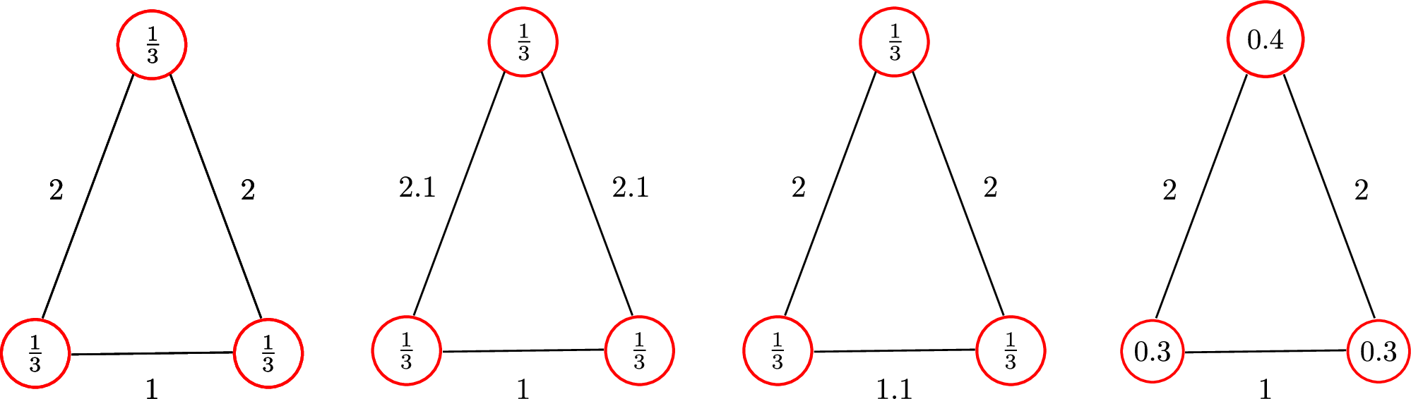
Refer to caption
Figure 6. Ultrametric measure spaces: Four non-isomorphic ultrametric measure spaces denoted (from left to right) as 𝒳i=(Xi,dXi,μXi)\mathcal{X}_{i}=(X_{i},d_{X_{i}},\mu_{X_{i}}), 1≤i≤41\leq i\leq 4.

6.3. Comparison of uGW,1u_{\mathrm{GW},1}, 𝐒𝐋𝐁1ult\mathbf{SLB}_{1}^{\mathrm{ult}}, dGW,1d_{\mathrm{GW},1} and 𝐒𝐋𝐁1\mathbf{SLB}_{1}

In the remainder of this section, we will demonstrate the differences between uGW,1u_{\mathrm{GW},1}, 𝐒𝐋𝐁1ult\mathbf{SLB}_{1}^{\mathrm{ult}}, dGW,1d_{\mathrm{GW},1} and 𝐒𝐋𝐁1\mathbf{SLB}_{1}. To this end, we first compare the metric measure spaces in Figure 6 based on dGW,1d_{\mathrm{GW},1} and 𝐒𝐋𝐁1\mathbf{SLB}_{1}. We observe that dGW,1d_{\mathrm{GW},1} (approximated in the same manner as uGW,1u_{\mathrm{GW},1}) and 𝐒𝐋𝐁1\mathbf{SLB}_{1} are hardly influenced by the differences between the ultrametric measure spaces 𝒳i\mathcal{X}_{i}, 1≤i≤41\leq i\leq 4. In particular, it is remarkable that dGW,1d_{\mathrm{GW},1} is affected the most by the changes made to the measure and not the metric structure (see Table 4 in Section E.2 for the complete results).

Next, we consider the differences between the aforementioned quantities more generally. For this purpose, we generate 4 ultrametric spaces ZkZ_{k}, 1≤k≤41\leq k\leq 4, with totally different dendrogram structures, whose diameters are between 0.5 and 0.6 (for the precise construction of these spaces see Section E.2). For each t=0,0.2,0.4,0.6t=0,0.2,0.4,0.6, we perturb each ZkZ_{k} independently to generate 15 ultrametric spaces Zk,tiZ^{i}_{k,t}, 1≤i≤151\leq i\leq 15, such that (Zk,ti)t≡(Zk)t(Z^{i}_{k,t})_{t}\equiv(Z_{k})_{t} for all ii. The spaces Zk,tiZ^{i}_{k,t} are called pertubations of ZkZ_{k} at level tt (see Figure 7 for an illustration and see Section E.2 for more details). The spaces Zk,tiZ^{i}_{k,t} are endowed with the uniform probability measure and we obtain a collection of ultrametric measure spaces 𝒵k,ti\mathcal{Z}^{i}_{k,t}. Naturally, we refer to kk as the class of the ultrametric measure space 𝒵k,ti\mathcal{Z}^{i}_{k,t}. We compute for each tt the quantities uGW,1u_{\mathrm{GW},1}, 𝐒𝐋𝐁1ult\mathbf{SLB}_{1}^{\mathrm{ult}}, dGW,1d_{\mathrm{GW},1} and 𝐒𝐋𝐁1\mathbf{SLB}_{1} among the resulting 6060 ultrametric measure spaces. The results, where the spaces have been ordered lexicographically by (k,i)(k,i), are visualized in Figure 8. As previously, we observe that uGW,1u_{\mathrm{GW},1} and 𝐒𝐋𝐁1ult\mathbf{SLB}_{1}^{\mathrm{ult}} as well as dGW,1d_{\mathrm{GW},1} and 𝐒𝐋𝐁1\mathbf{SLB}_{1} behave in a similar manner. More precisely, we see that both dGW,1d_{\mathrm{GW},1} and 𝐒𝐋𝐁1\mathbf{SLB}_{1} discriminate well between the different classes and that their behavior does not change too much for an increasing level of perturbation. On the other hand, uGW,1u_{\mathrm{GW},1} and 𝐒𝐋𝐁1ult\mathbf{SLB}_{1}^{\mathrm{ult}} are very sensitive to the level of perturbation. For small tt they discriminate better than dGW,1d_{\mathrm{GW},1} and 𝐒𝐋𝐁1\mathbf{SLB}_{1} between the different classes and pick up clearly that the perturbed spaces differ. However, if the level of perturbation becomes too large both quantities start to discriminate between spaces from the same class (see Figure 8).

Figure 7. Randomly sampled ultrametric measure spaces: Illustration of ZkZ_{k} for k=2,3,4,5k=2,3,4,5 (top row) and instances for perturbations of Z4Z_{4} with respect to perturbation level t∈{0,0.2,0.4,0.6}t\in\{0,0.2,0.4,0.6\} (bottom row).
Refer to caption
Figure 8. uGW,1/𝐒𝐋𝐁1ultu_{\mathrm{GW},1}/\mathbf{SLB}_{1}^{\mathrm{ult}} and dGW,1/𝐒𝐋𝐁1d_{\mathrm{GW},1}/\mathbf{SLB}_{1} among randomly generated ultrametric measure spaces: Heatmap representations of 𝐒𝐋𝐁1ult​(𝒵n,ti,𝒵n′,ti′)\mathbf{SLB}_{1}^{\mathrm{ult}}(\mathcal{Z}^{i}_{n,t},\mathcal{Z}^{i^{\prime}}_{n^{\prime},t}) (top row), uGW,1​(𝒵n,ti,𝒵n′,ti′)u_{\mathrm{GW},1}(\mathcal{Z}^{i}_{n,t},\mathcal{Z}^{i^{\prime}}_{n^{\prime},t}) (second row), 𝐒𝐋𝐁1​(𝒵n,ti,𝒵n′,ti′)\mathbf{SLB}_{1}(\mathcal{Z}^{i}_{n,t},\mathcal{Z}^{i^{\prime}}_{n^{\prime},t}) (third row) and dGW,1​(𝒵n,ti,𝒵n′,ti′)d_{\mathrm{GW},1}(\mathcal{Z}^{i}_{n,t},\mathcal{Z}^{i^{\prime}}_{n^{\prime},t}) (bottom row), k,k′∈{2,…,5}k,k^{\prime}\in\{2,\dots,5\} and i,i′∈{1,…,15}i,i^{\prime}\in\{1,\ldots,15\}.

In conclusion, uGW,1u_{\mathrm{GW},1} and 𝐒𝐋𝐁1ult\mathbf{SLB}_{1}^{\mathrm{ult}} are sensitive to differences in the large scales of the considered ultrametric measure spaces. While this leads (from small tt) to good discrimination in the above example, it also highlights that they are (different from dGW,1d_{\mathrm{GW},1} and 𝐒𝐋𝐁1\mathbf{SLB}_{1}) susceptible to large scale noise.

7. Phylogenetic tree shapes

Rooted phylogenetic trees (for a formal definition see e.g., [90]) are a common tool to visualize and analyze the evolutionary relationship between different organisms. In combination with DNA sequencing, they are an important tool to study the rapid evolution of different pathogens. It is well known that the (unweighted) shape of a phylogenetic tree, i.e., the tree’s connectivity structure without referring to its labels or the length of its branches, carries important information about macroevolutionary processes (see e.g., [72, 8, 27, 104]). In order to study the evolution of and the relation between different pathogens, it is of great interest to compare the shapes of phylogenetic trees created on the basis of different data sets. Currently, the number of tools for performing phylogenetic tree shape comparison is quite limited and the development of new methods for this is an active field of research [25, 73, 49, 60]. It is well known that certain classes of phylogenetic trees (as well as their respective tree shapes) can be identified as ultrametric spaces [90, Sec. 7]. On the other hand, general phylogenetic trees are closely related to treegrams (see Definition 5.3). In the following, we will use this connection and demonstrate exemplarily that the computationally efficient lower bound 𝐒𝐋𝐁1ult\mathbf{SLB}_{1}^{\mathrm{ult}} has some potential for comparing phylogenetic tree shapes. In particular, we contrast it to the metric defined for this application in Equation (4) of Colijn and Plazzotta 2018, in the following denoted as dCP,2d_{\mathrm{CP},2}, and study the behavior of 𝐒𝐋𝐁1\mathbf{SLB}_{1} in this framework.

Refer to caption
Figure 9. Transforming a phylogenetic tree shape into an ultra-dissimilarity space: In this figure, we illustrate the treegram corresponding to the ultra-dissimilarity space generated by Equation 26 with respect to the phylogenetic tree shape on the left. Note that the treegram preserves the tree structure and the smallest birth time of points is exactly 0.

In this section, we reconsider phylogenetic tree shape comparisons from Colijn and Plazzotta 2018 and thereby study HA protein sequences from human influenza A (H3N2) (data downloaded from NCBI on 22 January 2016). More precisely, we investigate the relation between two samples of size 200 of phylogenetic tree shapes with 500 tips. Phylogenetic trees from the first sample are based on a random subsample of size 500 of 2168 HA-sequences that were collected in the USA between March 2010 and September 2015, while trees from the second sample are based on a random subsample of size 500 of 1388 HA-sequences gathered in the tropics between January 2000 and October 2015 (for the exact construction of the trees see [25]). Although both samples of phylogenetic trees are based on HA protein sequences from human influenza A, we expect them to be quite different. On the one hand, influenza A is highly seasonal outside the tropics (where this seasonal variation is absent) with the majority of cases occurring in the winter [86]. On the other hand, it is well known that the undergoing evolution of the HA protein causes a ‘ladder-like’ shape of long-term influenza phylogenetic trees [51, 101, 103, 62] that is typically less developed in short term data sets. Thus, also the different collection period of the two data sets will most likely influence the respective phylogenetic tree shapes.

In order to compare the phylogenetic tree shapes of the resulting 400 trees, we have to transform the phylogenetic tree shapes into ultra-dissimilarity measure spaces 𝒳i=(Xi,uXi,μXi)\mathcal{X}_{i}=(X_{i},u_{X_{i}},\mu_{X_{i}}), 1≤i≤4001\leq i\leq 400. To this end, we discard all the lables, denote by XiX_{i} the tips of the ii’th phylogenetic tree and refer to the corresponding tree shape as 𝒯i\mathcal{T}_{i}. Next, we define the ultra-dissimilarities uXiu_{X_{i}} on XiX_{i}, 1≤i≤4001\leq i\leq 400. For this purpose, we set all edge length in the considered phylogenetic trees to one and construct uXiu_{X_{i}} as follows: let x1i,x2i∈Xix^{i}_{1},x^{i}_{2}\in X_{i} and let a1,2ia^{i}_{1,2} be the most recent common ancestor of x1ix^{i}_{1} and x2ix^{i}_{2}. Let da1,2id^{i}_{a_{1,2}} be the length of the shortest path from a1,2ia^{i}_{1,2} to the root, let d1id^{i}_{1} be the length of the shortest path from x1ix^{i}_{1} to the root and let did^{i} be the length of the longest shortest path from any tip to the root. Then, we define for any x1i,x2i∈Xix^{i}_{1},x^{i}_{2}\in X_{i}

(26) uXi​(x1i,x2i)={di−da1,2iif ​x1i≠x2idi−d1iif ​x1i=x2i,\addcontentsline{lla}{section}{\numberline q:treeshapedistance}u_{X_{i}}(x^{i}_{1},x^{i}_{2})=\begin{cases}d^{i}-d^{i}_{a_{1,2}}&\text{if }x^{i}_{1}\neq x^{i}_{2}\\ d^{i}-d^{i}_{1}&\text{if }x^{i}_{1}=x^{i}_{2},\end{cases}

and weight all tips in XiX_{i} equally (i.e. μXi\mu_{X_{i}} is the uniform measure on XiX_{i}). This naturally transforms the collection of phylogenetic tree shapes 𝒯i\mathcal{T}_{i}, 1≤i≤4001\leq i\leq 400, into a collection of ultra-dissimilarity spaces (see Figure 9 for an illustration), which allows us to directly apply 𝐒𝐋𝐁1ult\mathbf{SLB}_{1}^{\mathrm{ult}} to compare them (once again we exemplarily choose p=1p=1).

In Figure 10 we contrast our findings for the comparisons of the shapes 𝒯i\mathcal{T}_{i}, 1≤i≤4001\leq i\leq 400, to those obtained by computing the metric dCP,2d_{\mathrm{CP},2} described in [25]. The top row of Figure 10 visualizes the dissimilarity matrix for the comparisons of all 400 phylogenetic tree shapes (the first 200 entries correspond to the tree shapes from the US-influenza and the second 200 correspond to the ones from the tropic influenza) obtained by applying 𝐒𝐋𝐁1ult\mathbf{SLB}_{1}^{\mathrm{ult}} as heat map (left) and as multidimensional scaling plot (right). The heat map shows that the collection of US trees is divided into a large group 𝒢1≔(𝒯i)1≤i≤161\mathcal{G}_{1}\coloneqq(\mathcal{T}_{i})_{1\leq i\leq 161}, that is well separated from the phylogenetic tree shapes based on tropical data 𝒢3≔(𝒯i)201≤i≤400\mathcal{G}_{3}\coloneqq(\mathcal{T}_{i})_{201\leq i\leq 400}, and a smaller subgroup 𝒢2≔(𝒯i)162≤i≤200\mathcal{G}_{2}\coloneqq(\mathcal{T}_{i})_{162\leq i\leq 200}, that seems to be more similar (in the sense of 𝐒𝐋𝐁1ult\mathbf{SLB}_{1}^{\mathrm{ult}}) to the tropical phylogenetic tree shapes. In the following 𝒢1\mathcal{G}_{1} and 𝒢2\mathcal{G}_{2} are referred to as US main and US secondary group, respectively. This division is even more evident in the MDS-plot on the right (black points represent trees shapes from the US main group, blue points trees shapes from the US secondary group and red points trees shapes based on the tropical data).

We remark that in order to highlight the subgroups the US tree shapes have been reordered according to the output permutation of a single linkage dendrogram (w.r.t. 𝐒𝐋𝐁1ult\mathbf{SLB}_{1}^{\mathrm{ult}}) based on the US tree submatrix created by MATLAB 2019 and that the tropical tree shapes have been reordered analogously.

The second row of Figure 10 displays the analogous plots for dCP,2d_{\mathrm{CP},2}. It is noteworthy, that the coloring in the MDS-plot of the left is the same, i.e., T1∈𝒢1T_{1}\in\mathcal{G}_{1} is represented by a black point, T2∈𝒢2T_{2}\in\mathcal{G}_{2} by a blue one and T3∈𝒢3T_{3}\in\mathcal{G}_{3} by a red one. Interestingly, the analysis based on these plots differs from the previous one. Using dCP,2d_{\mathrm{CP},2} to compare the phylogenetic tree shapes at hand, we can split the data into two clusters, where one corresponds to the US data and the other one to the tropical data, with only a small overlap (see the MDS-plot in the second row of Figure 10 on the right). In particular, we notice that dCP,2d_{\mathrm{CP},2} does not clearly distinguish between the US groups 𝒢1\mathcal{G}_{1} and 𝒢2\mathcal{G}_{2}.

Refer to caption
Refer to caption
Figure 10. Phylogenetic tree shape comparison: Visualization of the dissimilarity matrices for the comparison of the phylogenetic tree shapes 𝒯i\mathcal{T}_{i}, 1≤i≤4001\leq i\leq 400, based on 𝐒𝐋𝐁1ult\mathbf{SLB}_{1}^{\mathrm{ult}} (top row) and dCP,2d_{\mathrm{CP},2} (bottom row) as heat maps (left) and MDS-plots (right).

In order to analyze the different findings of 𝐒𝐋𝐁1ult\mathbf{SLB}_{1}^{\mathrm{ult}} and dCP,2d_{\mathrm{CP},2}, we collect and compare different characteristics of the tree shapes in the groups 𝒢i\mathcal{G}_{i}, 1≤i≤31\leq i\leq 3. More precisely, we concentrate on various “metric” properties of the considered ultra-dissimilarity spaces like 15002​|𝒢i|​∑𝒯i∈𝒢i∑x,x′∈XiuXi​(x,x′)\frac{1}{500^{2}|\mathcal{G}_{i}|}\sum_{\mathcal{T}_{i}\in\mathcal{G}_{i}}\sum_{x,x^{\prime}\in X_{i}}u_{X_{i}}(x,x^{\prime}) (“mean average distance”) or 1|𝒢i|∑𝒯i∈𝒢imax{uXi(x,x′)|x,x′∈Xi}\frac{1}{|\mathcal{G}_{i}|}\sum_{\mathcal{T}_{i}\in\mathcal{G}_{i}}\max\{u_{X_{i}}(x,x^{\prime})|x,x^{\prime}\in X_{i}\} (“mean maximal distance”), 1≤i≤31\leq i\leq 3, (these influence 𝐒𝐋𝐁1ult\mathbf{SLB}_{1}^{\mathrm{ult}} strongly) as well as the mean numbers of certain connectivity structures, like the 4- and 5-structures (these influence dCP,2d_{\mathrm{CP},2}, for a formal definition see [25]). Theses values (see Table 1) show that the mean average distance and the mean maximal distance differ drastically between the two groups of the US tree shapes. The tree shapes in these two groups are completely different from a metric perspective and the values for the secondary US group strongly resemble those of the tropic tree shapes. On the other hand, the connectivity characteristics do not change too much between the US main and secondary group. Hence, the metric dCP,2d_{\mathrm{CP},2} does not clearly divide the US trees into two groups, although the differences are certainly present. When carefully checking the phylogenetic trees, the reasons for the differences between trees in the US main group and US secondary group are not immediately apparent. Nevertheless, it is remarkable that trees from the secondary US cluster generally contain more samples from California and Florida (on average 1.92 and 0.88 more) and less from Maryland, Kentucky and Washington (on average 0.73, 0.83 and 0.72 less).

USA (main group) USA (secondary group) Tropics
Mean Avg. Dist. 36.16 61.88 53.45
Mean Max. Dist. 56.12 86.13 94.26
Mean Num. of 4-Struc. 15.61 14.08 7.81
Mean Num. of 5-Struc. 28.04 27.97 35.82
Table 1. Tree shape characteristics: The means of several metric and connectivity characteristics of the ultra-dissimilarity spaces 𝒳i\mathcal{X}_{i} and the corresponding phylogenetic tree shapes 𝒯i\mathcal{T}_{i}, 1≤i≤4001\leq i\leq 400, for the three groups 𝒢i\mathcal{G}_{i}, 1≤i≤31\leq i\leq 3.

To conclude this section, we remark that using 𝐒𝐋𝐁1\mathbf{SLB}_{1} instead of 𝐒𝐋𝐁1ult\mathbf{SLB}_{1}^{\mathrm{ult}} for comparing the ultra-dissimilarity spaces 𝒳i\mathcal{X}_{i}, 1≤i≤4001\leq i\leq 400, gives comparable results (cf. Figure 11, coloring and ordering as previously). Nevertheless, we observe (as we already have in Section 6) that 𝐒𝐋𝐁1ult\mathbf{SLB}_{1}^{\mathrm{ult}} is more discriminating than 𝐒𝐋𝐁1\mathbf{SLB}_{1}. Furthermore, we mention that so far we have only considered unweighted phylogenetic tree shapes. However, the branch lengths of the considered phylogenetic trees are relevant in many examples, because they can for instance reflect the (inferred) genetic distance between evolutionary events [25]. While the branch lengths cannot easily be included in the metric dCP,2d_{\mathrm{CP},2}, the modeling of phylogenetic tree shapes as ultra-dissimilarity spaces is extremely flexible. It is straightforward to include branch lengths into the comparisons or to put emphasis on specific features (via weights on the corresponding tips). However, this is beyond the scope of this illustrative data analysis.

Refer to caption
Figure 11. Phylogenetic tree shape comparison based on 𝐒𝐋𝐁1\mathbf{SLB}_{1}: Representation of the dissimilarity matrices for the comparisons of the ultra-dissimilarity spaces 𝒳i\mathcal{X}_{i}, 1≤i≤4001\leq i\leq 400, based on 𝐒𝐋𝐁1\mathbf{SLB}_{1} as heat maps (left) and MDS-plots (right).

8. Concluding remarks

Since we suspect that computing uGW,pu_{\mathrm{GW},p} and uGW,psturmu_{\mathrm{GW},p}^{\mathrm{sturm}} for finite pp leads to NP-hard problems, it seems interesting to identify suitable collections of ultrametric measure spaces where these distances can be computed in polynomial time as done for the Gromov-Hausdorff distance in [70].

Acknowledgements

We are grateful to Prof. Colijn for sharing the data from [25] with us. F.M. and Z.W. acknowledge funding from the NSF under grants NSF CCF 1740761, NSF DMS 1723003, and NSF RI 1901360. A.M. and C.W. gratefully acknowledge support by the DFG Research Training Group 2088 and Cluster of Excellence MBExC 2067. F.M. and A.M. thank the Mathematisches Forschungsinstitut Oberwolfach. Conversations which eventually led to this project were initiated during the 2019 workshop “Statistical and Computational Aspects of Learning with Complex Structure”.

References

  • Adelson-Velskii and Kronrod [1945] Georgy M. Adelson-Velskii and Aleksandr S. Kronrod. About level sets of continuous functions with partial derivatives. In Dokl. Akad. Nauk SSSR, volume 49, pages 239–241, 1945.
  • Agarwal et al. [2018] Pankaj K. Agarwal, Kyle Fox, Abhinandan Nath, Anastasios Sidiropoulos, and Yusu Wang. Computing the Gromov-Hausdorff distance for metric trees. ACM Transactions on Algorithms (TALG), 14(2):1–20, 2018.
  • Aho and Hopcroft [1974] Alfred V. Aho and John E. Hopcroft. The design and analysis of computer algorithms. Pearson Education India, 1974.
  • Alvarez-Melis and Jaakkola [2018] David Alvarez-Melis and Tommi S. Jaakkola. Gromov-Wasserstein alignment of word embedding spaces. arXiv preprint arXiv:1809.00013, 2018.
  • Bartal [1996] Yair Bartal. Probabilistic approximation of metric spaces and its algorithmic applications. In Proceedings of 37th Conference on Foundations of Computer Science, pages 184–193. IEEE, 1996.
  • Billera et al. [2001] Louis J. Billera, Susan P. Holmes, and Karen Vogtmann. Geometry of the space of phylogenetic trees. Advances in Applied Mathematics, 27(4):733–767, 2001.
  • Billingsley [2013] Patrick Billingsley. Convergence of Probability Measures. John Wiley & Sons, 2013.
  • Blum and François [2006] Michael G.B. Blum and Olivier François. Which random processes describe the tree of life? A large-scale study of phylogenetic tree imbalance. Systematic Biology, 55(4):685–691, 2006.
  • Bonneel et al. [2015] Nicolas Bonneel, Julien Rabin, Gabriel Peyré, and Hanspeter Pfister. Sliced and radon Wasserstein barycenters of measures. Journal of Mathematical Imaging and Vision, 51(1):22–45, 2015.
  • Bottou et al. [2018] Leon Bottou, Martin Arjovsky, David Lopez-Paz, and Maxime Oquab. Geometrical insights for implicit generative modeling. In Braverman Readings in Machine Learning. Key Ideas from Inception to Current State, pages 229–268. Springer, 2018.
  • Brinkman and Olver [2012] Daniel Brinkman and Peter J. Olver. Invariant histograms. The American Mathematical Monthly, 119(1):4–24, 2012.
  • Bronstein et al. [2006a] Alexander M. Bronstein, Michael M. Bronstein, and Ron Kimmel. Efficient computation of isometry-invariant distances between surfaces. SIAM Journal on Scientific Computing, 28(5):1812–1836, 2006a.
  • Bronstein et al. [2006b] Alexander M. Bronstein, Michael M. Bronstein, and Ron Kimmel. Generalized multidimensional scaling: A framework for isometry-invariant partial surface matching. Proceedings of the National Academy of Sciences, 103(5):1168–1172, 2006b.
  • Bronstein et al. [2009a] Alexander M. Bronstein, Michael M. Bronstein, Alfred M. Bruckstein, and Ron Kimmel. Partial similarity of objects, or how to compare a centaur to a horse. International Journal of Computer Vision, 84(2):163, 2009a.
  • Bronstein et al. [2009b] Alexander M. Bronstein, Michael M. Bronstein, and Ron Kimmel. Topology-invariant similarity of nonrigid shapes. International journal of computer vision, 81(3):281, 2009b.
  • Bronstein et al. [2010] Alexander M. Bronstein, Michael M. Bronstein, Ron Kimmel, Mona Mahmoudi, and Guillermo Sapiro. A Gromov-Hausdorff framework with diffusion geometry for topologically-robust non-rigid shape matching. International Journal of Computer Vision, 89(2-3):266–286, 2010.
  • Brown et al. [2016] Peter Brown, Wayne Pullan, Yuedong Yang, and Yaoqi Zhou. Fast and accurate non-sequential protein structure alignment using a new asymmetric linear sum assignment heuristic. Bioinformatics, 32(3):370–377, 2016.
  • Bunne et al. [2019] Charlotte Bunne, David Alvarez-Melis, Andreas Krause, and Stefanie Jegelka. Learning generative models across incomparable spaces. arXiv preprint arXiv:1905.05461, 2019.
  • Carlsson and Mémoli [2010] Gunnar Carlsson and Facundo Mémoli. Characterization, stability and convergence of hierarchical clustering methods. Journal of machine learning research, 11(Apr):1425–1470, 2010.
  • Chazal et al. [2009] Frédéric Chazal, David Cohen-Steiner, Leonidas J Guibas, Facundo Mémoli, and Steve Y Oudot. Gromov-hausdorff stable signatures for shapes using persistence. In Proceedings of the Symposium on Geometry Processing, pages 1393–1403, 2009.
  • Chen and Safro [2011] Jie Chen and Ilya Safro. Algebraic distance on graphs. SIAM Journal on Scientific Computing, 33(6):3468–3490, 2011.
  • Chowdhury [2019] Samir Chowdhury. Metric and Topological Approaches to Network Data Analysis. PhD thesis, The Ohio State University, 2019.
  • Chowdhury and Mémoli [2019] Samir Chowdhury and Facundo Mémoli. The Gromov-Wasserstein distance between networks and stable network invariants. Information and Inference: A Journal of the IMA, 8(4):757–787, 2019.
  • Chowdhury and Needham [2020] Samir Chowdhury and Tom Needham. Generalized spectral clustering via Gromov-Wasserstein learning. arXiv preprint arXiv:2006.04163, 2020.
  • Colijn and Plazzotta [2018] Caroline Colijn and Giacomo Plazzotta. A metric on phylogenetic tree shapes. Systematic biology, 67(1):113–126, 2018.
  • David et al. [1997] Guy David, Stephen W. Semmes, Stephen Semmes, and Guy Rene Pierre Pierre. Fractured fractals and broken dreams: Self-similar geometry through metric and measure, volume 7. Oxford University Press, 1997.
  • Dayarian and Shraiman [2014] Adel Dayarian and Boris I. Shraiman. How to infer relative fitness from a sample of genomic sequences. Genetics, 197(3):913–923, 2014.
  • Do Ba et al. [2011] Khanh Do Ba, Huy L. Nguyen, Huy N. Nguyen, and Ronitt Rubinfeld. Sublinear time algorithms for Earth Mover’s distance. Theory of Computing Systems, 48(2):428–442, 2011.
  • Dong and Sawin [2020] Yihe Dong and Will Sawin. COPT: Coordinated optimal transport on graphs. arXiv preprint arXiv:2003.03892, 2020.
  • Dordovskyi et al. [2011] Dmitry Dordovskyi, Oleksiy Dovgoshey, and Eugeniy Petrov. Diameter and diametrical pairs of points in ultrametric spaces. P-Adic Numbers, Ultrametric Analysis, and Applications, 3(4):253–262, 2011.
  • Dudley [2018] Richard M. Dudley. Real analysis and probability. CRC Press, 2018.
  • Edwards [1975] David A. Edwards. The structure of superspace. In Studies in topology, pages 121–133. Elsevier, 1975.
  • Evans [2007] Steven N. Evans. Probability and Real Trees: École D’Été de Probabilités de Saint-Flour XXXV-2005. Springer, 2007.
  • Evans and Matsen [2012] Steven N. Evans and Frederick A. Matsen. The phylogenetic Kantorovich–Rubinstein metric for environmental sequence samples. Journal of the Royal Statistical Society: Series B (Statistical Methodology), 74(3):569–592, 2012.
  • Fakcharoenphol et al. [2004] Jittat Fakcharoenphol, Satish Rao, and Kunal Talwar. A tight bound on approximating arbitrary metrics by tree metrics. Journal of Computer and System Sciences, 69(3):485–497, 2004.
  • Folland [1999] Gerald B Folland. Real analysis: modern techniques and their applications, volume 40. John Wiley & Sons, 1999.
  • Gellert et al. [2019] Manuela Gellert, Md Faruq Hossain, Felix Jacob Ferdinand Berens, Lukas Willy Bruhn, Claudia Urbainsky, Volkmar Liebscher, and Christopher Horst Lillig. Substrate specificity of thioredoxins and glutaredoxins–towards a functional classification. Heliyon, 5(12):e02943, 2019.
  • Givens and Shortt [1984] Clark R. Givens and Rae Michael Shortt. A class of Wasserstein metrics for probability distributions. Michigan Math. J., 31(2):231–240, 1984. doi: 10.1307/mmj/1029003026. URL https://doi.org/10.1307/mmj/1029003026.
  • Greven et al. [2009] Andreas Greven, Peter Pfaffelhuber, and Anita Winter. Convergence in distribution of random metric measure spaces (λ\lambda-coalescent measure trees). Probability Theory and Related Fields, 145(1-2):285–322, 2009.
  • Grindstaff and Owen [2018] Gillian Grindstaff and Megan Owen. Geometric comparison of phylogenetic trees with different leaf sets. arXiv preprint arXiv:1807.04235, 2018.
  • Gromov [1981] M. Gromov. Groups of polynomial growth and expanding maps (with an appendix by Jacques Tits). Publications Mathématiques de l’IHÉS, 53:53–78, 1981.
  • Hein [1990] Jotun Hein. Reconstructing evolution of sequences subject to recombination using parsimony. Mathematical biosciences, 98(2):185–200, 1990.
  • Holm and Sander [1993] Liisa Holm and Chris Sander. Protein structure comparison by alignment of distance matrices. Journal of molecular biology, 233(1):123–138, 1993.
  • Howes [2012] Norman R. Howes. Modern analysis and topology. Springer Science & Business Media, 2012.
  • Jain and Dorai [2000] Anil K. Jain and Chitra Dorai. 3d object recognition: Representation and matching. Statistics and Computing, 10(2):167–182, 2000.
  • Jardine and Sibson [1971] Nicholas Jardine and Robin Sibson. Mathematical taxonomy. John Wiley & Sons, 1971.
  • Kantorovich [1942] Leonid V. Kantorovich. On the translocation of masses, cr (dokl.) acad. Sci. URSS (NS), 37:199, 1942.
  • Kantorovich and Rubinstein [1958] Leonid V. Kantorovich and G Rubinstein. On a space of completely additive functions (russ.). Vestnik Leningrad Univ, 13:52–59, 1958.
  • Kim et al. [2019] Jaehee Kim, Noah A. Rosenberg, and Julia A. Palacios. A metric space of ranked tree shapes and ranked genealogies. bioRxiv, 2019.
  • Kloeckner [2015] Benoît R. Kloeckner. A geometric study of Wasserstein spaces: Ultrametrics. Mathematika, 61(1):162–178, 2015.
  • Koelle et al. [2010] Katia Koelle, Priya Khatri, Meredith Kamradt, and Thomas B. Kepler. A two-tiered model for simulating the ecological and evolutionary dynamics of rapidly evolving viruses, with an application to influenza. Journal of The Royal Society Interface, 7(50):1257–1274, 2010.
  • Kolmogorov and Fomin [1957] Andreĭ N. Kolmogorov and Sergeĭ V. Fomin. Elements of the theory of functions and functional analysis, volume 1. Courier Corporation, 1957.
  • Kolouri et al. [2019] Soheil Kolouri, Kimia Nadjahi, Umut Simsekli, Roland Badeau, and Gustavo Rohde. Generalized sliced Wasserstein distances. In Advances in Neural Information Processing Systems, pages 261–272, 2019.
  • Kufareva and Abagyan [2011] Irina Kufareva and Ruben Abagyan. Methods of protein structure comparison. In Homology Modeling, pages 231–257. Springer, 2011.
  • Kuo et al. [2014] Hao-Yuan Kuo, Hong-Ren Su, Shang-Hong Lai, and Chin-Chia Wu. 3D object detection and pose estimation from depth image for robotic bin picking. In 2014 IEEE international conference on automation science and engineering (CASE), pages 1264–1269. IEEE, 2014.
  • Lafond et al. [2019] Manuel Lafond, Nadia El-Mabrouk, Katharina T. Huber, and Vincent Moulton. The complexity of comparing multiply-labelled trees by extending phylogenetic-tree metrics. Theoretical Computer Science, 760:15–34, 2019.
  • Le et al. [2019a] Tam Le, Nhat Ho, and Makoto Yamada. Fast tree variants of Gromov-Wasserstein. arXiv preprint arXiv:1910.04462, 2019a.
  • Le et al. [2019b] Tam Le, Makoto Yamada, Kenji Fukumizu, and Marco Cuturi. Tree-sliced variants of Wasserstein distances. In Advances in neural information processing systems, pages 12304–12315, 2019b.
  • Liebscher [2018] Volkmar Liebscher. New Gromov-inspired metrics on phylogenetic tree space. Bulletin of mathematical biology, 80(3):493–518, 2018.
  • Liu et al. [2020] Pengyu Liu, Matthew Gould, and Caroline Colijn. Polynomial phylogenetic analysis of tree shapes. BioRxiv, 2020.
  • Lowe [2001] David G. Lowe. Local feature view clustering for 3D object recognition. In Proceedings of the 2001 IEEE Computer Society Conference on Computer Vision and Pattern Recognition. CVPR 2001, volume 1, pages I–I. IEEE, 2001.
  • Łuksza and Lässig [2014] Marta Łuksza and Michael Lässig. A predictive fitness model for influenza. Nature, 507(7490):57–61, 2014.
  • Mallows [1972] Colin L. Mallows. A note on asymptotic joint normality. The Annals of Mathematical Statistics, pages 508–515, 1972.
  • MATLAB [2019] MATLAB. MATLAB: Accelerating the pace of engineering and science. The MathWorks, Inc., 2019. URL https://www.mathworks.com.
  • McGregor and Stubbs [2013] Andrew McGregor and Daniel Stubbs. Sketching Earth-Mover distance on graph metrics. In Approximation, Randomization, and Combinatorial Optimization. Algorithms and Techniques, pages 274–286. Springer, 2013.
  • Mémoli [2007] Facundo Mémoli. On the use of Gromov-Hausdorff distances for shape comparison. In M. Botsch, R. Pajarola, B. Chen, and M. Zwicker, editors, Eurographics Symposium on Point-Based Graphics. The Eurographics Association, 2007. ISBN 978-3-905673-51-7. doi: 10.2312/SPBG/SPBG07/081-090.
  • Mémoli [2011] Facundo Mémoli. Gromov-Wasserstein distances and the metric approach to object matching. Foundations of computational mathematics, 11(4):417–487, 2011.
  • Mémoli and Needham [2021] Facundo Mémoli and Tom Needham. Distance distributions and inverse problems for metric measure spaces. arXiv preprint arXiv:1810.09646, 2021.
  • Mémoli and Sapiro [2004] Facundo Mémoli and Guillermo Sapiro. Comparing point clouds. In Proceedings of the 2004 Eurographics/ACM SIGGRAPH symposium on Geometry processing, pages 32–40, 2004.
  • Mémoli et al. [2019] Facundo Mémoli, Zane Smith, and Zhengchao Wan. Gromov-Hausdorff distances on pp-metric spaces and ultrametric spaces. arXiv preprint arXiv:1912.00564, 2019.
  • Mézard et al. [1987] Marc Mézard, Giorgio Parisi, and Miguel Angel Virasoro. Spin glass theory and beyond: An Introduction to the Replica Method and Its Applications, volume 9. World Scientific Publishing Company, 1987.
  • Mooers and Heard [1997] Arne O. Mooers and Stephen B. Heard. Inferring evolutionary process from phylogenetic tree shape. The quarterly review of Biology, 72(1):31–54, 1997.
  • Morozov [2018] Alexey Anatolievich Morozov. Extension of Colijn-Plazotta tree shape distance metric to unrooted trees. BioRxiv, page 506022, 2018.
  • Morozov et al. [2013] Dmitriy Morozov, Kenes Beketayev, and Gunther Weber. Interleaving distance between merge trees. Discrete and Computational Geometry, 49(22-45):52, 2013.
  • Osada et al. [2002] Robert Osada, Thomas Funkhouser, Bernard Chazelle, and David Dobkin. Shape distributions. ACM Transactions on Graphics (TOG), 21(4):807–832, 2002.
  • Owen and Provan [2010] Megan Owen and J. Scott Provan. A fast algorithm for computing geodesic distances in tree space. IEEE/ACM Transactions on Computational Biology and Bioinformatics, 8(1):2–13, 2010.
  • Papazov et al. [2012] Chavdar Papazov, Sami Haddadin, Sven Parusel, Kai Krieger, and Darius Burschka. Rigid 3D geometry matching for grasping of known objects in cluttered scenes. The International Journal of Robotics Research, 31(4):538–553, 2012.
  • Pardalos and Vavasis [1991] Panos M. Pardalos and Stephen A. Vavasis. Quadratic programming with one negative eigenvalue is NP-hard. Journal of Global optimization, 1(1):15–22, 1991.
  • Peyré et al. [2016] Gabriel Peyré, Marco Cuturi, and Justin Solomon. Gromov-Wasserstein averaging of kernel and distance matrices. In International Conference on Machine Learning, pages 2664–2672, 2016.
  • Qiu [2009] Derong Qiu. Geometry of non-archimedean Gromov-Hausdorff distance. P-Adic Numbers, Ultrametric Analysis, and Applications, 1(4):317, 2009.
  • Rammal et al. [1986] Rammal Rammal, Gérard Toulouse, and Miguel A. Virasoro. Ultrametricity for physicists. Reviews of Modern Physics, 58:765–788, 1986.
  • Reeb [1946] Georges Reeb. Sur les points singuliers d’une forme de pfaff completement integrable ou d’une fonction numerique [on the singular points of a completely integrable pfaff form or of a numerical function]. Comptes Rendus Acad. Sciences Paris, 222:847–849, 1946.
  • Robinson [1971] David F. Robinson. Comparison of labeled trees with valency three. Journal of combinatorial theory, Series B, 11(2):105–119, 1971.
  • Robinson and Foulds [1981] David F. Robinson and Leslie R. Foulds. Comparison of phylogenetic trees. Mathematical biosciences, 53(1-2):131–147, 1981.
  • Rubner et al. [2000] Yossi Rubner, Carlo Tomasi, and Leonidas J. Guibas. The Earth Mover’s distance as a metric for image retrieval. International journal of computer vision, 40(2):99–121, 2000.
  • Russell et al. [2008] Colin A. Russell, Terry C. Jones, Ian G. Barr, Nancy J. Cox, Rebecca J. Garten, Vicky Gregory, Ian D. Gust, Alan W. Hampson, Alan J. Hay, Aeron C. Hurt, et al. The global circulation of seasonal influenza a (H3N2) viruses. Science, 320(5874):340–346, 2008.
  • Scetbon et al. [2021] Meyer Scetbon, Gabriel Peyré, and Marco Cuturi. Linear-time gromov wasserstein distances using low rank couplings and costs. arXiv preprint arXiv:2106.01128, 2021.
  • Schmiedl [2017] Felix Schmiedl. Computational aspects of the Gromov-Hausdorff distance and its application in non-rigid shape matching. Discret. Comput. Geom., 57(4):854–880, 2017. doi: 10.1007/s00454-017-9889-4. URL https://doi.org/10.1007/s00454-017-9889-4.
  • Semmes [2007] Stephen Semmes. An introduction to the geometry of ultrametric spaces. arXiv preprint arXiv:0711.0709, 2007.
  • Semple et al. [2003] Charles Semple, Mike Steel, et al. Phylogenetics, volume 24. Oxford University Press on Demand, 2003.
  • Smith et al. [2016] Zane Smith, Samir Chowdhury, and Facundo Mémoli. Hierarchical representations of network data with optimal distortion bounds. In 2016 50th Asilomar Conference on Signals, Systems and Computers, pages 1834–1838. IEEE, 2016.
  • Sturm [2006] Karl-Theodor Sturm. On the geometry of metric measure spaces. Acta mathematica, 196(1):65–131, 2006.
  • Sturm [2012] Karl-Theodor Sturm. The space of spaces: Curvature bounds and gradient flows on the space of metric measure spaces. arXiv preprint arXiv:1208.0434, 2012.
  • Thorsley and Klavins [2008] David Thorsley and Eric Klavins. Model reduction of stochastic processes using Wasserstein pseudometrics. In 2008 American Control Conference, pages 1374–1381. IEEE, 2008.
  • Titouan et al. [2019] Vayer Titouan, Nicolas Courty, Romain Tavenard, and Rémi Flamary. Optimal transport for structured data with application on graphs. In International Conference on Machine Learning, pages 6275–6284, 2019.
  • Touli and Wang [2018] Elena Farahbakhsh Touli and Yusu Wang. FPT-algorithms for computing Gromov-Hausdorff and interleaving distances between trees. arXiv preprint arXiv:1811.02425, 2018.
  • Vallender [1974] Sergei S. Vallender. Calculation of the Wasserstein distance between probability distributions on the line. Theory of Probability & Its Applications, 18(4):784–786, 1974.
  • Vayer et al. [2019] Titouan Vayer, Rémi Flamary, Romain Tavenard, Laetitia Chapel, and Nicolas Courty. Sliced Gromov-Wasserstein. arXiv preprint arXiv:1905.10124, 2019.
  • Villani [2003] Cédric Villani. Topics in optimal transportation. American Mathematical Soc., 2003.
  • Villani [2008] Cédric Villani. Optimal transport: Old and new, volume 338. Springer Science & Business Media, 2008.
  • Volz et al. [2013] Erik M. Volz, Katia Koelle, and Trevor Bedford. Viral phylodynamics. PLoS Comput Biol, 9(3):e1002947, 2013.
  • Wan [2020] Zhengchao Wan. A novel construction of Urysohn universal ultrametric space via the Gromov-Hausdorff ultrametric. arXiv preprint arXiv:2007.08105, 2020.
  • Westgeest et al. [2012] Kim B. Westgeest, Miranda de Graaf, Mathieu Fourment, Theo M. Bestebroer, Ruud van Beek, Monique I.J. Spronken, Jan C. de Jong, Guus F Rimmelzwaan, Colin A. Russell, Albert D.M.E. Osterhaus, et al. Genetic evolution of the neuraminidase of influenza a (H3N2) viruses from 1968 to 2009 and its correspondence to haemagglutinin evolution. The Journal of general virology, 93(Pt 9):1996, 2012.
  • Wu and Choi [2016] Taoyang Wu and Kwok Pui Choi. On joint subtree distributions under two evolutionary models. Theoretical population biology, 108:13–23, 2016.
  • Zarichnyi [2005] Ihor Zarichnyi. Gromov-Hausdorff ultrametric. arXiv preprint math/0511437, 2005.

Appendix A Missing details from Section 2

A.1. Proofs from Section 2

In this section we give the proofs of various results form Section 2.

A.1.1. Proof of Theorem 2.2

Recall that for a given θ∈𝒟⁡(X)\theta\in\mathcal{D}(X), we define uθ:X×X→ℝ≥0u_{\theta}:X\times X\rightarrow\mathbb{R}_{\geq 0} as follows

uθ​(x,x′)≔inf{t≥0|x​ and ​x′​ belong to the same block of ​θ​(t)}.u_{\theta}(x,x^{\prime})\coloneqq\inf\{t\geq 0|\,x\text{ and }x^{\prime}\text{ belong to the same block of }\theta(t)\}.

It is straightforward to verify that uθu_{\theta} is an ultrametric. For any Cauchy sequence {xn}n∈ℕ\{x_{n}\}_{n\in\mathbb{N}} in (X,uθ)(X,u_{\theta}), let Di≔supm,n≥iuθ​(xm,xn)D_{i}\coloneqq\sup_{m,n\geq i}u_{\theta}(x_{m},x_{n}) for each i∈ℕi\in\mathbb{N}. Then, each Di<∞D_{i}<\infty and limi→∞Di=0\lim_{i\rightarrow\infty}D_{i}=0. By definition of uθu_{\theta}, we have that for each i∈ℕi\in\mathbb{N} the set {xn}n=i∞\{x_{n}\}_{n=i}^{\infty} is contained in the block [xi]Di∈θ⁡(Di)[x_{i}]_{D_{i}}\in\theta(D_{i}). Let Xi≔[xi]DiX_{i}\coloneqq[x_{i}]_{D_{i}} for each i∈ℕi\in\mathbb{N}. Then, obviously we have that Xj⊆XiX_{j}\subseteq X_{i} for any 1≤i<j1\leq i<j. By condition (7) in Definition 2.1, we have that ⋂i∈ℕXi≠∅\bigcap_{i\in\mathbb{N}}X_{i}\neq\emptyset. Choose x∗∈⋂i∈ℕXix_{*}\in\bigcap_{i\in\mathbb{N}}X_{i}, then it is easy to verify that x∗=limn→∞xnx_{*}=\lim_{n\rightarrow\infty}x_{n} and thus (X,uθ)(X,u_{\theta}) is a complete space. To prove that (X,uθ)(X,u_{\theta}) is a compact space, we need to verify that for each t>0t>0, XtX_{t} is a finite space (cf. Lemma A.7). Since θ⁡(t)\theta(t) is finite by condition (6) in Definition 2.1, we have that Xt={[x]t|x∈X}=θ⁡(t)X_{t}=\{[x]_{t}|\,x\in X\}=\theta(t) is finite and thus XX is compact. Therefore, we have proved that uθ∈𝒰⁡(X)u_{\theta}\in\mathcal{U}(X). Based on this, the map ΔX:𝒟⁡(X)→𝒰⁡(X)\Delta_{X}:\mathcal{D}(X)\to\mathcal{U}(X) by θ↦uθ\theta\mapsto u_{\theta} is well-defined.

Now given u∈𝒰⁡(X)u\in\mathcal{U}(X), we define a map θu:[0,∞)→𝐏𝐚𝐫𝐭⁡(X)\theta_{u}:[0,\infty)\rightarrow\mathbf{Part}(X) as follows: for each t≥0t\geq 0, consider the equivalence relation ∼t\sim_{t} with respect to uu, i.e., x∼tx′x\sim_{t}x^{\prime} if and only if u⁡(x,x′)≤tu(x,x^{\prime})\leq t. This is actually the same equivalence relation defined in Section 2.2 for introducing quotient ultrametric spaces. We then let θu​(t)\theta_{u}(t) to be the partition induced by ∼t\sim_{t}, i.e., θu​(t)=Xt.\theta_{u}(t)=X_{t}. It is not hard to show that θu\theta_{u} satisfies conditions (1)–(5) in Definition 2.1. Since XX is compact, then θu​(t)=Xt\theta_{u}(t)=X_{t} is finite for each t>0t>0 and thus θu\theta_{u} satisfies condition (6) in Definition 2.1. Now, let {tn}n∈ℕ\{t_{n}\}_{n\in\mathbb{N}} be a decreasing sequence such that limn→∞tn=0\lim_{n\rightarrow\infty}t_{n}=0 and let Xn∈θX​(tn)X_{n}\in\theta_{X}(t_{n}) such that for any 1≤n<m1\leq n<m, Xm⊆XnX_{m}\subseteq X_{n}. Since each Xn=[xn]tnX_{n}=[x_{n}]_{t_{n}} for some xn∈Xx_{n}\in X, XnX_{n} is a compact subset of XX. Since XX is also complete, we have that ⋂n∈ℕXn≠∅\bigcap_{n\in\mathbb{N}}X_{n}\neq\emptyset. Therefore, θu\theta_{u} satisfies condition (7) in Definition 2.1 and thus θu∈𝒟⁡(X)\theta_{u}\in\mathcal{D}(X). Then, we define the map ΥX:𝒰⁡(X)→𝒟⁡(X)\Upsilon_{X}:\mathcal{U}(X)\to\mathcal{D}(X) by u↦θuu\mapsto\theta_{u}.

It is easy to check that ΥX\Upsilon_{X} is the inverse of ΔX\Delta_{X} and thus we have established that ΔX:𝒟⁡(X)→𝒰⁡(X)\Delta_{X}:\mathcal{D}(X)\rightarrow\mathcal{U}(X) is bijective.

A.1.2. Proof of Lemma 2.8

First of all, we show that the right hand side of Equation 16 is well defined. More precisely, we employ Lemma A.7 to prove that the supremum

supB∈V⁡(X)\{X}​ and ​α​(B)≠β⁡(B)diam⁡(B∗)\sup_{B\in V(X)\backslash\{X\}\,\text{ and }\,\alpha(B)\neq\beta(B)}\mathrm{diam}\left(B^{*}\right)

is attained. For arbitrary B0∈V⁡(X)\{X}B_{0}\in V(X)\backslash\{X\} such that α⁡(B0)≠β⁡(B0)\alpha(B_{0})\neq\beta(B_{0}), we have that diam⁡(B0∗)>0\mathrm{diam}\left(B^{*}_{0}\right)>0. By Lemma A.7 the spaces XtX_{t} are finite for t>0t>0. Since V(X)={[x]t|x∈X,t>0}=⋃t>0XtV(X)=\{[x]_{t}|\,x\in X,t>0\}=\bigcup_{t>0}X_{t}, there are only finitely many B∈V⁡(X)\{X}B\in V(X)\backslash\{X\} such that diam⁡(B)≥diam⁡(B0∗)\mathrm{diam}\left(B\right)\geq\mathrm{diam}\left(B^{*}_{0}\right) and thus diam⁡(B∗)≥diam⁡(B0∗)\mathrm{diam}\left(B^{*}\right)\geq\mathrm{diam}\left(B^{*}_{0}\right). This implies that the supremum is attained and thus

(27) supB∈V⁡(X)\{X}​ and ​α​(B)≠β⁡(B)diam⁡(B∗)=maxB∈V⁡(X)\{X}​ and ​α​(B)≠β⁡(B)⁡diam⁡(B∗).\addcontentsline{lla}{section}{\numberline q:winfinitymax}\sup_{B\in V(X)\backslash\{X\}\,\text{ and }\,\alpha(B)\neq\beta(B)}\mathrm{diam}\left(B^{*}\right)=\max_{B\in V(X)\backslash\{X\}\,\text{ and }\,\alpha(B)\neq\beta(B)}\mathrm{diam}\left(B^{*}\right).

Let B1B_{1} denote the maximizer in Equation 27 and let δ≔diam⁡(B1∗)\delta\coloneqq\mathrm{diam}\left(B_{1}^{*}\right). It is easy to see that for any x∈Xx\in X, α⁡([x]δ)=β⁡([x]δ)\alpha([x]_{\delta})=\beta([x]_{\delta}).

By Strassen’s theorem (see for example [31, Theorem 11.6.2]),

(28) dW,∞(α,β)=inf{r≥0|for any closed subset A⊆X,α(A)≤β(Ar)},\addcontentsline{lla}{section}{\numberline q:strassen}d_{\mathrm{W},\infty}(\alpha,\beta)=\inf\{r\geq 0|\,\text{for any closed subset }A\subseteq X,\,\alpha(A)\leq\beta(A^{r})\},

where Ar≔{x∈X|uX​(x,A)≤r}A^{r}\coloneqq\{x\in X|\,u_{X}(x,A)\leq r\}.

Since α⁡(B1)≠β⁡(B1)\alpha(B_{1})\neq\beta(B_{1}), we assume without loss of generality that α⁡(B1)>β⁡(B1)\alpha(B_{1})>\beta(B_{1}). By definition of B1∗B_{1}^{*}, it is obvious that (B1)δ=B1∗(B_{1})^{\delta}=B_{1}^{*} (recall: δ≔diam⁡(B1∗)\delta\coloneqq\mathrm{diam}\left(B_{1}^{*}\right)) and (B1)r=B1(B_{1})^{r}=B_{1} for all 0≤r<δ0\leq r<\delta. Therefore, α⁡(B1)≤β⁡((B1)r)\alpha(B_{1})\leq\beta((B_{1})^{r}) only when r≥δr\geq\delta. By Equation 28, this implies that dW,∞​(α,β)≥δd_{\mathrm{W},\infty}(\alpha,\beta)\geq\delta. Conversely, for any closed set AA, we have that Aδ=⋃x∈A[x]δA^{\delta}=\bigcup_{x\in A}[x]_{\delta}. For two closed balls in ultrametric spaces, either one includes the other or they have no intersection. Therefore, there exists a subset S⊆AS\subseteq A such that [x]δ∩[x′]δ=∅[x]_{\delta}\cap[x^{\prime}]_{\delta}=\emptyset for all x,x′∈Sx,x^{\prime}\in S and x≠x′x\neq x^{\prime}, and that Aδ=⨆x∈S[x]δA^{\delta}=\bigsqcup_{x\in S}[x]_{\delta}. Then, α⁡(A)≤α⁡(Aδ)=∑x∈Sα⁡([x]δ)=∑x∈Sβ⁡([x]δ)=β⁡(Aδ)\alpha(A)\leq\alpha(A^{\delta})=\sum_{x\in S}\alpha([x]_{\delta})=\sum_{x\in S}\beta([x]_{\delta})=\beta(A^{\delta}). Hence, dW,∞​(α,β)≤δd_{\mathrm{W},\infty}(\alpha,\beta)\leq\delta and thus

dW,∞​(α,β)=maxB∈V⁡(X)\{X}​ and ​α​(B)≠β⁡(B)⁡diam⁡(B∗).d_{\mathrm{W},\infty}(\alpha,\beta)=\max_{B\in V(X)\backslash\{X\}\text{ and }\alpha(B)\neq\beta(B)}\mathrm{diam}\left(B^{*}\right).

A.2. Technical issues from Section 2

In the following, we address various technical issues from Section 2.

A.2.1. Synchronized rooted trees

A synchronized rooted tree, is a combinatorial tree T=(V,E)T=(V,E) with a root o∈Vo\in V and a height function h:V→[0,∞)h:V\rightarrow[0,\infty) such that h−1​(0)h^{-1}(0) coincides with the leaf set and h⁡(v)<h⁡(v∗)h(v)<h(v^{*}) for each v∈V\{o}v\in V\backslash\{o\}, where v∗v^{*} is the parent of vv. Similar as in Theorem 2.2 that there exists a correspondence between ultrametric spaces and dendrograms, an ultrametric space XX uniquely determines a synchronized rooted tree TXT_{X} [50].

Now given a compact ultrametric space (X,uX)(X,u_{X}), we construct the corresponding sychronized rooted tree TXT_{X} via the dendrogram θX\theta_{X} associated with uXu_{X}. Recall from Section 2.3 that V⁡(X)≔⋃t>0θX​(t)V(X)\coloneqq\bigcup_{t>0}\theta_{X}(t). For each B∈V⁡(X)\{X}B\in V(X)\backslash\{X\}, denote by B∗B^{*} the smallest element in V⁡(X)V(X) such that B⫋B∗B\subsetneqq B^{*}, whose existence is guaranteed by the following lemma:

Lemma A.1.

Let XX be a compact ultrametric space and let V⁡(X)=⋃t>0θX​(t)V(X)=\bigcup_{t>0}\theta_{X}(t), where θX\theta_{X} is as defined in Remark 2.3. For each B∈V⁡(X)B\in V(X) such that B≠XB\neq X, there exists B∗∈V⁡(X)B^{*}\in V(X) such that B∗≠BB^{*}\neq B and B∗⊆B′B^{*}\subseteq B^{\prime} for all B′∈V⁡(X)B^{\prime}\in V(X) with B⫋B′B\subsetneqq B^{\prime}.

Proof.

Let δ≔diam⁡(B)\delta\coloneqq\mathrm{diam}\left(B\right). Let x∈Bx\in B, then B=[x]δB=[x]_{\delta}. By Lemma A.7, XδX_{\delta} is a finite set. Consider δ∗≔min⁡{uXδ​([x]δ,[x′]δ)|[x′]δ≠[x]δ}\delta^{*}\coloneqq\min\{u_{X_{\delta}}([x]_{\delta},[x^{\prime}]_{\delta})|\,[x^{\prime}]_{\delta}\neq[x]_{\delta}\}. Let B∗≔[x]δ∗B^{*}\coloneqq[x]_{\delta^{*}}, then B∗B^{*} is the smallest element in V⁡(X)V(X) containing BB under inclusion. Indeed, B∗≠BB^{*}\neq B and if B⊆B′B\subseteq B^{\prime} for some B′∈V⁡(X)B^{\prime}\in V(X), then B′=[x]rB^{\prime}=[x]_{r} for some r>δr>\delta. It is easy to see that for all δ<r<δ∗\delta<r<\delta^{*}, [x]r=[x]δ[x]_{r}=[x]_{\delta}. Therefore, if B′≠BB^{\prime}\neq B, we must have that r≥δ∗r\geq\delta^{*} and thus B∗=[x]δ∗⊆[x]r=B′B^{*}=[x]_{\delta^{*}}\subseteq[x]_{r}=B^{\prime}. ∎

Now, we define a combinatorial tree TX=(VX,EX)T_{X}=(V_{X},E_{X}) as follows: we let VX≔V⁡(X)V_{X}\coloneqq V(X); for any distinct B,B′∈VXB,B^{\prime}\in V_{X}, we let (B,B′)∈EX(B,B^{\prime})\in E_{X} iff either B=(B′)∗B=(B^{\prime})^{*} or B′=B∗B^{\prime}=B^{*}. We choose X∈VXX\in V_{X} to be the root of TXT_{X}, then any B≠XB\neq X in VXV_{X} has a unique parent B∗B^{*}. We define hX:VX→[0,∞)h_{X}:V_{X}\rightarrow[0,\infty) such that hX​(B)≔diam⁡(B)2h_{X}(B)\coloneqq\frac{\mathrm{diam}\left(B\right)}{2} for any B∈VXB\in V_{X}. Now, TXT_{X} endowed with the root XX and the height function hXh_{X} is a synchronized rooted tree. It is easy to see that XX can be isometrically identified with hX−1​(0)h_{X}^{-1}(0) of the so-called metric completion of TXT_{X} (see [50, Section 2.3] for details). With this construction Theorem 2.7 follows directly from [50, Lemma 3.1].

A.3. dW,p(ℝ≥0,Λ∞)d^{(\mathbb{R}_{\geq 0},\Lambda_{\infty})}_{\mathrm{W},p} between compactly supported measures

Next, we demonstrate that Theorem 2.9 extends naturally to the case of compactly supported probability measures in (ℝ≥0,Λ∞)(\mathbb{R}_{\geq 0},\Lambda_{\infty}). For this purpose, it is important to note that compact subsets of (ℝ≥0,Λ∞)(\mathbb{R}_{\geq 0},\Lambda_{\infty}) have a very particular structure as shown by the subsequent lemma.

Lemma A.2.

Let X⊆(ℝ≥0,Λ∞)X\subseteq\mathbb{(}\mathbb{R}_{\geq 0},\Lambda_{\infty}). XX is a compact subset if and only if XX is either a finite set or a countable set with 00 being the unique cluster point (w.r.t. the usual Euclidean distance Λ1\Lambda_{1}).

Proof.

If XX is finite, then obviously XX is compact. Assume that XX is a countable set with 00 being the unique cluster point (w.r.t. the usual Euclidean distance Λ1\Lambda_{1}). If {xn}n∈ℕ⊆X\{x_{n}\}_{n\in\mathbb{N}}\subseteq X is a Cauchy sequence with respect to Λ∞\Lambda_{\infty}, then either xnx_{n} is a constant when nn is large or limn→∞xn=0\lim_{n\rightarrow\infty}x_{n}=0. In either case, the limit of {xn}n∈ℕ\{x_{n}\}_{n\in\mathbb{N}} belongs to XX and thus XX is complete. Now for any ε>0\varepsilon>0, by Lemma A.7, XεX_{\varepsilon} is a finite set. Denote Xε={[x1]ε,…,[xn]ε}X_{\varepsilon}=\{[x_{1}]_{\varepsilon},\ldots,[x_{n}]_{\varepsilon}\}. Then, {x1,…,xn}\{x_{1},\ldots,x_{n}\} is a finite ε\varepsilon-net of XX. Therefore, XX is totally bounded and thus XX is compact.

Now, assume that XX is compact. Then, for any ε>0\varepsilon>0, XεX_{\varepsilon} is a finite set. Suppose Xε={[x1]ε,…,[xn]ε}X_{\varepsilon}=\{[x_{1}]_{\varepsilon},\ldots,[x_{n}]_{\varepsilon}\} where 0≤x1<x2<⋯<xn0\leq x_{1}<x_{2}<\cdots<x_{n}. Further, we have that Λ∞​(xi,xj)=xj\Lambda_{\infty}(x_{i},x_{j})=x_{j} whenever 1≤i<j≤n1\leq i<j\leq n. This implies that

  1. (1)

    xi>εx_{i}>\varepsilon for all 2≤i≤n2\leq i\leq n;

  2. (2)

    [xi]ε={xi}[x_{i}]_{\varepsilon}=\{x_{i}\} for all 2≤i≤n2\leq i\leq n.

Therefore, X∩(ε,∞)={x2,…,xn}X\cap(\varepsilon,\infty)=\{x_{2},\ldots,x_{n}\} is a finite set. Since ε>0\varepsilon>0 is arbitrary, XX is an at most countable set and has no cluster point (w.r.t. the usual Euclidean distance Λ1\Lambda_{1}) other than 00. If XX is countable, then 00 must be a cluster point and by compactness of XX, we have that 0∈X0\in X. ∎

Based on the special structure of compact subsets of (ℝ≥0,Λ∞)(\mathbb{R}_{\geq 0},\Lambda_{\infty}), we derive the following extension of Theorem 2.9.

Theorem A.3 (dW,p(ℝ≥0,Λ∞)d^{(\mathbb{R}_{\geq 0},\Lambda_{\infty})}_{\mathrm{W},p} between compactly supported measures).

Suppose α,β\alpha,\beta are supported on a countable subset X≔{0}∪{xi|i∈ℕ}X\coloneqq\{0\}\cup\{x_{i}|\,i\in\mathbb{N}\} of ℝ≥0\mathbb{R}_{\geq 0} such that 0<…<xn<xn−1<…<x10<\ldots<x_{n}<x_{n-1}<\ldots<x_{1} and 00 is the only cluster point with respect to the usual Euclidean distance. Let αi≔α⁡({xi})\alpha_{i}\coloneqq\alpha(\{x_{i}\}) for i∈ℕi\in\mathbb{N} and α0≔α⁡({0})\alpha_{0}\coloneqq\alpha(\{0\}). Similarly, let βi≔β⁡({xi})\beta_{i}\coloneqq\beta(\{x_{i}\}) and β0≔β⁡({0})\beta_{0}\coloneqq\beta(\{0\}). Then for p∈[1,∞)p\in[1,\infty),

(29) dW,p(ℝ≥0,Λ∞)​(α,β)=2−1p​(∑i=2∞|∑j=i∞(αj−βj)|⋅|xi−1p−xip|+∑i=1∞|αi−βi|⋅xip)1p.\addcontentsline{lla}{section}{\numberline q:dp}d^{(\mathbb{R}_{\geq 0},\Lambda_{\infty})}_{\mathrm{W},p}(\alpha,\beta)=2^{-\frac{1}{p}}\left(\sum_{i=2}^{\infty}\left|\sum_{j=i}^{\infty}(\alpha_{j}-\beta_{j})\right|\cdot|x_{i-1}^{p}-x_{i}^{p}|+\sum_{i=1}^{\infty}|\alpha_{i}-\beta_{i}|\cdot x_{i}^{p}\right)^{\frac{1}{p}}.

Let FαF_{\alpha} and FβF_{\beta} denote the cumulative distribution functions of α\alpha and β\beta, respectively. Then, we obtain

dW,∞(ℝ≥0,Λ∞)​(α,β)=max⁡(max2≤i<∞,Fα​(xi)≠Fβ​(xi)⁡xi−1,max1≤i<∞,αi≠βi⁡xi).d_{\mathrm{W},\infty}^{(\mathbb{R}_{\geq 0},\Lambda_{\infty})}(\alpha,\beta)=\max\left(\max_{2\leq i<\infty,F_{\alpha}(x_{i})\neq F_{\beta}(x_{i})}x_{i-1},\max_{1\leq i<\infty,\alpha_{i}\neq\beta_{i}}x_{i}\right).
Proof.

Note that V⁡(X)={{0}∪{xj|j≥i}|i∈ℕ}∪{{xi}|i∈ℕ}V(X)=\{\{0\}\cup\{x_{j}|\,j\geq i\}|\,i\in\mathbb{N}\}\cup\{\{x_{i}\}|\,i\in\mathbb{N}\} (recall that each set corresponds to a closed ball). Thus, we conclude the proof by applying Lemma 2.7 and Lemma 2.8. ∎

A.3.1. Closed-form solution for dW,p(ℝ≥0,Λq)d_{\mathrm{W},p}^{(\mathbb{R}_{\geq 0},\Lambda_{q})}

In the following, we will derive the subsequent theorem.

Theorem A.4.

Given 1≤p,q<∞1\leq p,q<\infty and two compactly supported probability measures α\alpha and β\beta on ℝ≥0\mathbb{R}_{\geq 0}, we have that

dW,p(ℝ≥0,Λq)​(α,β)≤(∫01Λq​(Fα−1​(t),Fβ−1​(t))p​𝑑t)1p.d_{\mathrm{W},p}^{(\mathbb{R}_{\geq 0},\Lambda_{q})}(\alpha,\beta)\leq\left(\int_{0}^{1}\Lambda_{q}(F_{\alpha}^{-1}(t),F_{\beta}^{-1}(t))^{p}dt\right)^{\frac{1}{p}}.

When q≤pq\leq p, the equality holds whereas when q>pq>p, the equality does not hold in general.

One important ingredient for the proof of Theorem A.4 is Lemma 3.2 of Chowdhury and Mémoli 2019 which we restate here for convenience.

Lemma A.5 (Chowdhury and Mémoli 2019).

Let X,YX,Y be two Polish metric spaces and let f:X→ℝf:X\rightarrow\mathbb{R} and g:Y→ℝg:Y\rightarrow\mathbb{R} be measurable maps. Denote by f×g:X×Y→ℝ2f\times g:X\times Y\rightarrow\mathbb{R}^{2} the map (x,y)↦(f⁡(x),g⁡(y))(x,y)\mapsto(f(x),g(y)). Then, for any μY∈𝒫⁡(X)\mu_{Y}\in\mathcal{P}(X) and μY∈𝒫⁡(Y)\mu_{Y}\in\mathcal{P}(Y)

(f×g)#​𝒞​(μX,μY)=𝒞⁡(f#​μY,g#​μY).(f\times g)_{\#}\mathcal{C}(\mu_{X},\mu_{Y})=\mathcal{C}(f_{\#}\mu_{Y},g_{\#}\mu_{Y}).

Based on Lemma A.5, we can show the following auxiliary result.

Lemma A.6.

Let 1≤q≤p<∞1\leq q\leq p<\infty. Assume that α\alpha and β\beta are compactly supported probability measures on ℝ≥0\mathbb{R}_{\geq 0}. Then,

(dW,p(ℝ≥0,Λq)​(α,β))p=(dW,pq(ℝ≥0,Λ1)​((Sq)#​α,(Sq)#​β))pq,\left(d_{\mathrm{W},p}^{(\mathbb{R}_{\geq 0},\Lambda_{q})}(\alpha,\beta)\right)^{p}=\left(d_{\mathrm{W},\frac{p}{q}}^{(\mathbb{R}_{\geq 0},\Lambda_{1})}((S_{q})_{\#}\alpha,(S_{q})_{\#}\beta)\right)^{\frac{p}{q}},

where Sq:ℝ≥0→ℝ≥0S_{q}:\mathbb{R}_{\geq 0}\rightarrow\mathbb{R}_{\geq 0} taking xx to xqx^{q} is the qq-snowflake transform defined in Section 3.3.

Proof.
(dW,p(ℝ≥0,Λq)​(α,β))p\displaystyle\left(d_{\mathrm{W},p}^{(\mathbb{R}_{\geq 0},\Lambda_{q})}(\alpha,\beta)\right)^{p} =infμ∈𝒞⁡(α,β)∫ℝ≥0×ℝ≥0(Λq​(x,y))p​μ​(𝑑x×𝑑y)\displaystyle=\inf_{\mu\in\mathcal{C}(\alpha,\beta)}\int_{\mathbb{R}_{\geq 0}\times\mathbb{R}_{\geq 0}}(\Lambda_{q}(x,y))^{p}\mu(dx\times dy)
=infμ∈𝒞⁡(α,β)∫ℝ≥0×ℝ≥0|Sq​(x)−Sq​(y)|pq​μ​(𝑑x×𝑑y)\displaystyle=\inf_{\mu\in\mathcal{C}(\alpha,\beta)}\int_{\mathbb{R}_{\geq 0}\times\mathbb{R}_{\geq 0}}|S_{q}(x)-S_{q}(y)|^{\frac{p}{q}}\mu(dx\times dy)
=infμ∈𝒞⁡(α,β)∫ℝ≥0×ℝ≥0|s−t|pq​(Sq×Sq)#​μ​(𝑑s×𝑑t)\displaystyle=\inf_{\mu\in\mathcal{C}(\alpha,\beta)}\int_{\mathbb{R}_{\geq 0}\times\mathbb{R}_{\geq 0}}|s-t|^{\frac{p}{q}}(S_{q}\times S_{q})_{\#}\mu(ds\times dt)
=(dW,pq(ℝ≥0,Λ1)​((Sq)#​α,(Sq)#​β))pq,\displaystyle=\left(d_{\mathrm{W},\frac{p}{q}}^{(\mathbb{R}_{\geq 0},\Lambda_{1})}((S_{q})_{\#}\alpha,(S_{q})_{\#}\beta)\right)^{\frac{p}{q}},

where we use pq≥1\frac{p}{q}\geq 1 and Lemma A.5 in the last equality. ∎

With Lemma A.6 at our disposal, we can demonstrate Theorem A.4.

Proof of Theorem A.4.

We first note that dW,p(ℝ≥0,Λq)​(α,β)=inf(ξ,η)(𝔼⁡(Λq​(ξ,η)p))1pd_{\mathrm{W},p}^{(\mathbb{R}_{\geq 0},\Lambda_{q})}(\alpha,\beta)=\inf_{(\xi,\eta)}\big(\mathbb{E}(\Lambda_{q}(\xi,\eta)^{p})\big)^{\frac{1}{p}}, where ξ\xi and η\eta are two random variables with marginal distributions α\alpha and β\beta, respectively. Moreover, let ζ\zeta be the random variable uniformly distributed on [0,1][0,1], then Fα−1​(ζ)F_{\alpha}^{-1}(\zeta) has distribution function FαF_{\alpha} and Fβ−1​(ζ)F_{\beta}^{-1}(\zeta) has distribution function FβF_{\beta} (see for example Vallender 1974). Let ξ=Fα−1​(ζ)\xi=F_{\alpha}^{-1}(\zeta) and η=Fβ−1​(ζ)\eta=F_{\beta}^{-1}(\zeta), then we have

dW,p(ℝ≥0,Λq)​(α,β)≤(𝔼⁡(Λq​(ξ,η)p))1p=(∫01Λq​(Fα−1​(t),Fβ−1​(t))p​𝑑t)1p.d_{\mathrm{W},p}^{(\mathbb{R}_{\geq 0},\Lambda_{q})}(\alpha,\beta)\leq\big(\mathbb{E}(\Lambda_{q}(\xi,\eta)^{p})\big)^{\frac{1}{p}}=\left(\int_{0}^{1}\Lambda_{q}(F_{\alpha}^{-1}(t),F_{\beta}^{-1}(t))^{p}dt\right)^{\frac{1}{p}}.

Next, we assume that q≤pq\leq p. By Lemma A.6, we have that

(dW,p(ℝ≥0,Λq)​(α,β))p=(dW,pq(ℝ≥0,Λ1)​((Sq)#​α,(Sq)#​β))pq.\displaystyle\left(d_{\mathrm{W},p}^{(\mathbb{R}_{\geq 0},\Lambda_{q})}(\alpha,\beta)\right)^{p}=\left(d_{\mathrm{W},\frac{p}{q}}^{(\mathbb{R}_{\geq 0},\Lambda_{1})}((S_{q})_{\#}\alpha,(S_{q})_{\#}\beta)\right)^{\frac{p}{q}}.

Then,

(dW,pq(ℝ≥0,Λ1)​((Sq)#​α,(Sq)#​β))pq=∫01|Fα,q−1​(t)−Fβ,q−1​(t)|pq​𝑑t,\left(d_{\mathrm{W},\frac{p}{q}}^{(\mathbb{R}_{\geq 0},\Lambda_{1})}((S_{q})_{\#}\alpha,(S_{q})_{\#}\beta)\right)^{\frac{p}{q}}=\int_{0}^{1}|F_{\alpha,q}^{-1}(t)-F_{\beta,q}^{-1}(t)|^{\frac{p}{q}}dt,

where Fα,qF_{\alpha,q} and Fβ,qF_{\beta,q} are distribution functions of (Sq)#​α(S_{q})_{\#}\alpha and (Sq)#​β(S_{q})_{\#}\beta, respectively. It is easy to verify that Fα,q​(t)=(Fα−1​(t))qF_{\alpha,q}(t)=(F_{\alpha}^{-1}(t))^{q} and Fβ,q​(t)=(Fβ−1​(t))qF_{\beta,q}(t)=(F_{\beta}^{-1}(t))^{q}. Therefore,

dW,p(ℝ≥0,Λq)​(α,β)=(∫01Λq​(Fα−1​(t),Fβ−1​(t))p​𝑑t)1pd_{\mathrm{W},p}^{(\mathbb{R}_{\geq 0},\Lambda_{q})}(\alpha,\beta)=\left(\int_{0}^{1}\Lambda_{q}(F_{\alpha}^{-1}(t),F_{\beta}^{-1}(t))^{p}dt\right)^{\frac{1}{p}}

Finally, we demonstrate that for q>pq>p the equality does not hold in general. We first consider the extreme case p=1p=1 and q=∞q=\infty (though we require q<∞q<\infty in the assumptions of the theorem, we relax this for now). Let α0=12​δ1+12​δ2\alpha_{0}=\frac{1}{2}\delta_{1}+\frac{1}{2}\delta_{2} and β0=12​δ2+12​δ3\beta_{0}=\frac{1}{2}\delta_{2}+\frac{1}{2}\delta_{3} where δx\delta_{x} means the Dirac measure at point x∈ℝ≥0x\in\mathbb{R}_{\geq 0}. Then, we have that

dW,1(ℝ≥0,Λ∞)​(α0,β0)=32<52=∫01Λ∞​(Fα−1​(t),Fβ−1​(t))​𝑑t.d_{\mathrm{W},1}^{(\mathbb{R}_{\geq 0},\Lambda_{\infty})}(\alpha_{0},\beta_{0})=\frac{3}{2}<\frac{5}{2}=\int_{0}^{1}\Lambda_{\infty}(F_{\alpha}^{-1}(t),F_{\beta}^{-1}(t))dt.

It is not hard to see that both dW,p(ℝ≥0,Λq)​(α0,β0)d_{\mathrm{W},p}^{(\mathbb{R}_{\geq 0},\Lambda_{q})}(\alpha_{0},\beta_{0}) and (∫01Λq​(Fα−1​(t),Fβ−1​(t))p​𝑑t)1p\left(\int_{0}^{1}\Lambda_{q}(F_{\alpha}^{-1}(t),F_{\beta}^{-1}(t))^{p}dt\right)^{\frac{1}{p}} are continuous with respect to p∈[1,∞)p\in[1,\infty) and q∈[1,∞]q\in[1,\infty]. Then, for pp close to 1 and q<∞q<\infty large enough, and in particular, p<qp<q, we have that

dW,p(ℝ≥0,Λq)​(α0,β0)<(∫01Λq​(Fα−1​(t),Fβ−1​(t))p​𝑑t)1p.d_{\mathrm{W},p}^{(\mathbb{R}_{\geq 0},\Lambda_{q})}(\alpha_{0},\beta_{0})<\left(\int_{0}^{1}\Lambda_{q}(F_{\alpha}^{-1}(t),F_{\beta}^{-1}(t))^{p}dt\right)^{\frac{1}{p}}.

∎

A.3.2. Miscellaneous

In the remainder of this section, we collect several technical results that find implicit or explicit usage throughout Section 2.

Lemma A.7.

Let XX be a complete ultrametric space. Then, XX is compact ultrametric space if and only if for any t>0t>0, XtX_{t} is a finite space.

Proof.

Wan 2020 proves that whenever XX is compact, XtX_{t} is finite for any t>0t>0.

Conversely, we assume that XtX_{t} is finite for any t>0t>0. We only need to prove that XX is totally bounded. For any ε>0\varepsilon>0, XεX_{\varepsilon} is a finite set and thus there exists x1,…,xn∈Xx_{1},\ldots,x_{n}\in X such that Xε={[x1]ε,…,[xn]ε}.X_{\varepsilon}=\left\{[x_{1}]_{\varepsilon},\ldots,[x_{n}]_{\varepsilon}\right\}. Now, for any x∈Xx\in X, there exists xix_{i} for some i=1,…,ni=1,\ldots,n such that x∈[xi]εx\in[x_{i}]_{\varepsilon}. This implies that uX​(x,xi)≤εu_{X}(x,x_{i})\leq\varepsilon. Therefore, the set {x1,…,xn}⊆X\{x_{1},\ldots,x_{n}\}\subseteq X is an ε\varepsilon-net of XX. Then, XX is totally bounded and thus compact. ∎

Lemma A.8.

V⁡(X)V(X) is the collection of all closed balls in XX except for singletons {x}\{x\} such that xx is a cluster point in XX. In particular, X∈V⁡(X)X\in V(X) and for any x∈Xx\in X, if xx is not a cluster point, then {x}∈V⁡(X)\{x\}\in V(X).

Proof.

Given any t>0t>0 and x∈Xx\in X, [x]t=Bt​(x)={x′∈X|uX​(x,x′)≤t}[x]_{t}=B_{t}(x)=\{x^{\prime}\in X|\,u_{X}(x,x^{\prime})\leq t\}. Therefore, V⁡(X)V(X) is a collection of closed balls in XX. On the contrary, any closed ball Bt​(x)B_{t}(x) with positive radius t>0t>0 coincides with [x]t∈θX​(t)[x]_{t}\in\theta_{X}(t) and thus belongs to V⁡(X)V(X). Now, for any singleton {x}=B0​(x)\{x\}=B_{0}(x). If xx is not a cluster point, then there exists t>0t>0 such that Bt​(x)={x}B_{t}(x)=\{x\} which implies that {x}∈V⁡(X)\{x\}\in V(X). If xx is a cluster point, then for any t>0t>0, {x}⫋Bt​(x)=[x]t\{x\}\subsetneqq B_{t}(x)=[x]_{t}. In particular, this implies that {x}≠[x]t\{x\}\neq[x]_{t} for all t>0t>0 and thus {x}∉V⁡(X)\{x\}\notin V(X). In conclusion, V⁡(X)V(X) is the collection of all closed balls in XX except for singletons {x}\{x\} such that xx is a cluster point in XX.

If XX is a one point space, then obviously X∈V⁡(X)={X}X\in V(X)=\{X\}. Otherwise, let δ≔diam⁡(X)>0\delta\coloneqq\mathrm{diam}\left(X\right)>0, then for any x∈Xx\in X we have that X=[x]δ∈V⁡(X)X=[x]_{\delta}\in V(X). As for singletons {x}\{x\} where x∈Xx\in X is not a cluster point, we have proved above that {x}∈V⁡(X)\{x\}\in V(X). ∎

Appendix B Missing details from Section 3

B.1. Proofs from Section 3.1

Next, we give the missing proofs of the results stated in Section 3.1.

B.1.1. Proof of Proposition 3.3

  1. (1)

    This directly follows from the definitions of uGW,psturmu_{\mathrm{GW},p}^{\mathrm{sturm}} and dGW,psturmd_{\mathrm{GW},p}^{\mathrm{sturm}} (see Equation 10 and Equation 5).

  2. (2)

    This simply follows from Jensen’s inequality.

  3. (3)

    By (2), we know that {uGW,nsturm​(𝒳,𝒴)}n∈ℕ\{u_{\mathrm{GW},n}^{\mathrm{sturm}}(\mathcal{X},\mathcal{Y})\}_{n\in\mathbb{N}} is an increasing sequence with a finite upper bound uGW,∞sturm​(𝒳,𝒴)u_{\mathrm{GW},\infty}^{\mathrm{sturm}}(\mathcal{X},\mathcal{Y}). Therefore, L≔limn→∞uGW,nsturm​(𝒳,𝒴)L\coloneqq\lim_{n\rightarrow\infty}u_{\mathrm{GW},n}^{\mathrm{sturm}}(\mathcal{X},\mathcal{Y}) exists and L≤uGW,∞sturm​(𝒳,𝒴)L\leq u_{\mathrm{GW},\infty}^{\mathrm{sturm}}(\mathcal{X},\mathcal{Y}).

    Next, we come to the opposite inequality. By Proposition B.1, there exist un∈𝒟ult​(uX,uY)u_{n}\in\mathcal{D}^{\mathrm{ult}}(u_{X},u_{Y}) and μn∈𝒞⁡(μX,μY)\mu_{n}\in\mathcal{C}(\mu_{X},\mu_{Y}) such that

    (∫X×Y(un​(x,y))n​μn​(𝑑x×𝑑y))1n=uGW,nsturm​(𝒳,𝒴).\left(\int_{X\times Y}(u_{n}(x,y))^{n}\mu_{n}(dx\times dy)\right)^{\frac{1}{n}}=u_{\mathrm{GW},n}^{\mathrm{sturm}}(\mathcal{X},\mathcal{Y}).

    By Lemma B.19 and Lemma B.21, the sequence {un}n∈ℕ\{u_{n}\}_{n\in\mathbb{N}} uniformly converges to some u∈𝒟ult​(uX,uY)u\in\mathcal{D}^{\mathrm{ult}}(u_{X},u_{Y}) and {μn}n∈ℕ\{\mu_{n}\}_{n\in\mathbb{N}} weakly converges to some μ∈𝒞⁡(μX,μY)\mu\in\mathcal{C}(\mu_{X},\mu_{Y}) (after taking appropriate subsequences of both sequences). Let M:=sup(x,y)∈supp⁡(μ)u⁡(x,y)M:=\sup_{(x,y)\in\mathrm{supp}\left(\mu\right)}u(x,y). Let ε>0\varepsilon>0 and let U={(x,y)∈X×Y|u⁡(x,y)>M−ε}.U=\{(x,y)\in X\times Y\,|\,u(x,y)>M-\varepsilon\}. Then, μ⁡(U)>0\mu(U)>0. Since UU is open, it follows that there exists a small ε1>0\varepsilon_{1}>0 such that μn​(U)>μ⁡(U)−ε1>0\mu_{n}(U)>\mu(U)-\varepsilon_{1}>0 for all nn large enough (see e.g. Billingsley 2013). Moreover, by uniform convergence of the sequence {un}n∈ℕ\{u_{n}\}_{n\in\mathbb{N}}, we have |u⁡(x,y)−un​(x,y)|≤ε|u(x,y)-u_{n}(x,y)|\leq\varepsilon for any (x,y)∈X×Y(x,y)\in X\times Y when nn is large enough. Therefore, we obtain for nn large enough

    (∫X×Y(un​(x,y))n​μn​(𝑑x×𝑑y))1n≥(μn​(U))1n​(M−2​ε)≥(μ⁡(U)−ε1)1n​(M−2​ε).\displaystyle\left(\int_{X\times Y}(u_{n}(x,y))^{n}\mu_{n}(dx\times dy)\right)^{\frac{1}{n}}\geq(\mu_{n}(U))^{\frac{1}{n}}(M-2\varepsilon)\geq(\mu(U)-\varepsilon_{1})^{\frac{1}{n}}(M-2\varepsilon).

    Letting n→∞n\rightarrow\infty, we obtain L≥M−2​εL\geq M-2\varepsilon. Since ε>0\varepsilon>0 is arbitrary, we obtain L≥M≥uGW,∞sturm​(𝒳,𝒴)L\geq M\geq u_{\mathrm{GW},\infty}^{\mathrm{sturm}}(\mathcal{X},\mathcal{Y}).

B.1.2. Proof of Theorem 3.4

In this section, we devote to prove Theorem 3.4. To this end, we will first verify the existence of optimal metrics and optimal couplings in Equation 18.

Proposition B.1 (Existence of optimal couplings).

Let 𝒳=(X,uX,μX)\mathcal{X}=\left(X,u_{X},\mu_{X}\right) and 𝒴=(Y,uY,μY)\mathcal{Y}=\left(Y,u_{Y},\mu_{Y}\right) be compact ultrametric measure spaces. Then, there always exist u∈𝒟ult​(uX,uY)u\in\mathcal{D}^{\mathrm{ult}}(u_{X},u_{Y}) and μ∈𝒞⁡(μX,μY)\mu\in\mathcal{C}(\mu_{X},\mu_{Y}) such that for 1≤p<∞1\leq p<\infty

uGW,psturm​(𝒳,𝒴)=(∫X×Y(u⁡(x,y))p​μ​(𝑑x×𝑑y))1pu_{\mathrm{GW},p}^{\mathrm{sturm}}(\mathcal{X},\mathcal{Y})=\left(\int_{X\times Y}(u(x,y))^{p}\mu(dx\times dy)\right)^{\frac{1}{p}}

and such that

uGW,∞sturm​(𝒳,𝒴)=sup(x,y)∈supp⁡(μ)u⁡(x,y).u_{\mathrm{GW},\infty}^{\mathrm{sturm}}(\mathcal{X},\mathcal{Y})=\sup_{(x,y)\in\mathrm{supp}\left(\mu\right)}u(x,y).
Proof.

The following proof is a suitable adaptation from proof of Lemma 3.3 in [92]. We will only prove the claim for the case p<∞p<\infty since the case p=∞p=\infty can be shown in a similar manner. Let un∈𝒟ult​(uX,uY)u_{n}\in\mathcal{D}^{\mathrm{ult}}(u_{X},u_{Y}) and μn∈𝒞⁡(μX,μY)\mu_{n}\in\mathcal{C}(\mu_{X},\mu_{Y}) be such that

(∫X×Y(un​(x,y))p​μn​(𝑑x×𝑑y))1p≤uGW,psturm​(𝒳,𝒴)+1n.\left(\int_{X\times Y}(u_{n}(x,y))^{p}\mu_{n}(dx\times dy)\right)^{\frac{1}{p}}\leq u_{\mathrm{GW},p}^{\mathrm{sturm}}(\mathcal{X},\mathcal{Y})+\frac{1}{n}.

By Lemma B.19, {μn}n∈ℕ\{\mu_{n}\}_{n\in\mathbb{N}} weakly converges (after taking an appropriate subsequence) to some μ∈𝒞⁡(μX,μY)\mu\in\mathcal{C}(\mu_{X},\mu_{Y}). By Lemma B.21, {un}n∈ℕ\{u_{n}\}_{n\in\mathbb{N}} uniformly converges (after taking an appropriate subsequence) to some u∈𝒟ult​(uX,uY)u\in\mathcal{D}^{\mathrm{ult}}(u_{X},u_{Y}). Then, it is easy to verify that

(∫X×Y(u⁡(x,y))p​μ​(𝑑x×𝑑y))1p≤uGW,psturm​(𝒳,𝒴).\left(\int_{X\times Y}(u(x,y))^{p}\mu(dx\times dy)\right)^{\frac{1}{p}}\leq u_{\mathrm{GW},p}^{\mathrm{sturm}}(\mathcal{X},\mathcal{Y}).

∎

As a direct consequence of the proposition, we get the subsequent result.

Corollary B.2.

Fix 1≤p≤∞1\leq p\leq\infty. Let 𝒳=(X,uX,μX)\mathcal{X}=\left(X,u_{X},\mu_{X}\right) and 𝒴=(Y,uY,μY)\mathcal{Y}=\left(Y,u_{Y},\mu_{Y}\right) be compact ultrametric measure spaces. Then, there exist a compact ultrametric space ZZ and isometric embeddings ϕ:X↪Z\phi:X\hookrightarrow Z and ψ:Y↪Z\psi:Y\hookrightarrow Z such that

uGW,psturm​(𝒳,𝒴)=dW,pZ​(ϕ#​μX,ψ#​μY).u_{\mathrm{GW},p}^{\mathrm{sturm}}(\mathcal{X},\mathcal{Y})=d_{\mathrm{W},p}^{Z}(\phi_{\#}\mu_{X},\psi_{\#}\mu_{Y}).

Before we come to the proof of Theorem 3.4, it remains to establish another auxiliary result. We ensure that the Wasserstein pseudometric of order pp on a compact pseudo-ultrametric space (X,uX)(X,u_{X}) is for p∈[1,∞)p\in[1,\infty) a pp-pseudometric and for p=∞p=\infty a pseudo-ultrametric, i.e., we prove for 1≤p<∞1\leq p<\infty that for all α1,α2,α3∈𝒫⁡(X)\alpha_{1},\alpha_{2},\alpha_{3}\in\mathcal{P}(X)

dW,p(X,uX)​(μ1,μ3)≤((dW,p(X,uX)​(μ1,μ2))p+(dW,p(X,uX)​(μ2,μ3))p)1/pd_{\mathrm{W},p}^{(X,u_{X})}(\mu_{1},\mu_{3})\leq\left(\left(d_{\mathrm{W},p}^{(X,u_{X})}(\mu_{1},\mu_{2})\right)^{p}+\left(d_{\mathrm{W},p}^{(X,u_{X})}(\mu_{2},\mu_{3})\right)^{p}\right)^{1/p}

and for p=∞p=\infty that for all α1,α2,α3∈𝒫⁡(X)\alpha_{1},\alpha_{2},\alpha_{3}\in\mathcal{P}(X)

dW,p(X,uX)​(μ1,μ3)≤max⁡(dW,p(X,uX)​(μ1,μ2),dW,p(X,uX)​(μ2,μ3)).d_{\mathrm{W},p}^{(X,u_{X})}(\mu_{1},\mu_{3})\leq\max\left(d_{\mathrm{W},p}^{(X,u_{X})}(\mu_{1},\mu_{2}),d_{\mathrm{W},p}^{(X,u_{X})}(\mu_{2},\mu_{3})\right).
Lemma B.3.

Let (X,uX)(X,u_{X}) be a compact pseudo-ultrametric space. Then, for 1≤p≤∞1\leq p\leq\infty the pp-Wasserstein metric dW,p(X,uX)d_{\mathrm{W},p}^{(X,u_{X})} is a pp-pseudometric on 𝒫⁡(X)\mathcal{P}(X). In particular, when p=∞p=\infty, it is an pseudo-ultrametric on 𝒫⁡(X)\mathcal{P}(X).

Proof.

We prove the statement by adapting the proof of the triangle inequality for the pp-Wasserstein distance (see e.g., [99, Theorem 7.3]). We only prove the case when p<∞p<\infty whereas the case p=∞p=\infty follows by analogous arguments.

Let α1,α2,α3∈𝒫⁡(X)\alpha_{1},\alpha_{2},\alpha_{3}\in\mathcal{P}(X), denote by μ12\mu_{12} an optimal transport plan between α1\alpha_{1} and α2\alpha_{2} and by μ23\mu_{23} an optimal transport plan between α2\alpha_{2} and α3\alpha_{3} (see [100, Theorem 4.1] for the existence of μ12\mu_{12} and μ23\mu_{23}). Furthermore, let XiX_{i} be the support of αi\alpha_{i}, 1≤i≤31\leq i\leq 3. Then, by the Gluing Lemma [99, Lemma 7.6] there exists a measure μ∈𝒫⁡(X1×X2×X3)\mu\in\mathcal{P}(X_{1}\times X_{2}\times X_{3}) with marginals μ12\mu_{12} on X1×X2X_{1}\times X_{2} and μ23\mu_{23} on X2×X3X_{2}\times X_{3}. Clearly, we obtain

(dW,p(X,uX)​(α1,α3))p≤∫X1×X2×X3uXp​(x,z)​μ​(𝑑x×𝑑y×𝑑z)\displaystyle\left(d_{\mathrm{W},p}^{(X,u_{X})}(\alpha_{1},\alpha_{3})\right)^{p}\leq\int_{X_{1}\times X_{2}\times X_{3}}\!u_{X}^{p}\left(x,z\right)\,\mu(dx\times dy\times dz)
≤∫X1×X2×X3(uXp​(x,y)+uXp​(y,z))​μ​(𝑑x×𝑑y×𝑑z).\displaystyle\leq\int_{X_{1}\times X_{2}\times X_{3}}\!\left(u_{X}^{p}\left(x,y\right)+u_{X}^{p}\left(y,z\right)\right)\,\mu(dx\times dy\times dz).

Here, we used that uXu_{X} is an ultrametric, i.e., in particular a pp-metric [70, Proposition 1.16]. With this we obtain that

(dW,p(X,uX)​(α1,α2))p≤∫X1×X2uXp​(x,y)​μ12​(𝑑x×𝑑y)+∫X2×X3uXp​(y,z)​μ23​(𝑑y×𝑑z)\displaystyle\left(d_{\mathrm{W},p}^{(X,u_{X})}(\alpha_{1},\alpha_{2})\right)^{p}\leq\int_{X_{1}\times X_{2}}\!u_{X}^{p}\left(x,y\right)\,\mu_{12}(dx\times dy)+\int_{X_{2}\times X_{3}}\!u_{X}^{p}\left(y,z\right)\,\mu_{23}(dy\times dz)
=(dW,p(X,uX)​(α1,α2))p+(dW,p(X,uX)​(α2,α3))p.\displaystyle=\left(d_{\mathrm{W},p}^{(X,u_{X})}(\alpha_{1},\alpha_{2})\right)^{p}+\left(d_{\mathrm{W},p}^{(X,u_{X})}(\alpha_{2},\alpha_{3})\right)^{p}.

∎

With Proposition B.1 and Lemma B.3 at our disposal we are now ready to prove Theorem 3.4 which states that uGW,psturmu_{\mathrm{GW},p}^{\mathrm{sturm}} is indeed a pp-metric on 𝒰w\mathcal{U}^{w}.

Proof of Theorem 3.4.

It is clear that uGW,psturmu_{\mathrm{GW},p}^{\mathrm{sturm}} is symmetric and that uGW,psturm​(𝒳,𝒴)=0u_{\mathrm{GW},p}^{\mathrm{sturm}}(\mathcal{X},\mathcal{Y})=0 if 𝒳≅w𝒴\mathcal{X}\cong_{w}\mathcal{Y}. Furthermore, we remark that uGW,psturm​(𝒳,𝒴)≥dGW,psturm​(𝒳,𝒴)u_{\mathrm{GW},p}^{\mathrm{sturm}}(\mathcal{X},\mathcal{Y})\geq d_{\mathrm{GW},p}^{\mathrm{sturm}}(\mathcal{X},\mathcal{Y}) by Proposition 3.3. Since dGW,psturm​(𝒳,𝒴)=0d_{\mathrm{GW},p}^{\mathrm{sturm}}(\mathcal{X},\mathcal{Y})=0 implies that 𝒳≅w𝒴\mathcal{X}\cong_{w}\mathcal{Y} ([93]), we have that uGW,psturm​(𝒳,𝒴)=0u_{\mathrm{GW},p}^{\mathrm{sturm}}(\mathcal{X},\mathcal{Y})=0 implies that 𝒳≅w𝒴\mathcal{X}\cong_{w}\mathcal{Y}. It remains to verify the pp-triangle inequality. To this end, we only prove the case when p<∞p<\infty whereas the case p=∞p=\infty follows by analogous arguments.

Let 𝒳,𝒴,𝒵∈𝒰w\mathcal{X},\mathcal{Y},\mathcal{Z}\in\mathcal{U}^{w}. Suppose uX​Y∈𝒟ult​(uX,uY)u_{XY}\in\mathcal{D}^{\mathrm{ult}}(u_{X},u_{Y}) and uY​Z∈𝒟ult​(uY,uZ)u_{YZ}\in\mathcal{D}^{\mathrm{ult}}(u_{Y},u_{Z}) are optimal metric couplings such that

(uGW,psturm​(𝒳,𝒴))p=(dW,p(X⊔Y,uX​Y)​(μX,μY))p​ and ​(uGW,psturm​(𝒴,𝒵))p=(dW,p(Y⊔Z,uY​Z)​(μY,μZ))p.\left(u_{\mathrm{GW},p}^{\mathrm{sturm}}(\mathcal{X},\mathcal{Y})\right)^{p}=\left(d_{\mathrm{W},p}^{(X\sqcup Y,u_{XY})}(\mu_{X},\mu_{Y})\right)^{p}\text{ and }\left(u_{\mathrm{GW},p}^{\mathrm{sturm}}(\mathcal{Y},\mathcal{Z})\right)^{p}=\left(d_{\mathrm{W},p}^{(Y\sqcup Z,u_{YZ})}(\mu_{Y},\mu_{Z})\right)^{p}.

Further, define uX​Y​Zu_{XYZ} on X⊔Y⊔ZX\sqcup Y\sqcup Z as

uX​Y​Z​(x1,x2)={uX​Y​(x1,x2)x1,x2∈X⊔YuY​Z​(x1,x2)x1,x2∈Y⊔Zinf{max⁡(uX​Y​(x1,y),uY​Z​(y,x2))|y∈Y}x1∈X,x2∈Zinf{max⁡(uX​Y​(x2,y),uY​Z​(y,x1))|y∈Y}x1∈Z,x2∈X.u_{XYZ}(x_{1},x_{2})=\begin{cases}u_{XY}(x_{1},x_{2})&x_{1},x_{2}\in X\sqcup Y\\ u_{YZ}(x_{1},x_{2})&x_{1},x_{2}\in Y\sqcup Z\\ \inf\{\max(u_{XY}(x_{1},y),u_{YZ}(y,x_{2}))\,|\,y\in Y\}&x_{1}\in X,x_{2}\in Z\\ \inf\{\max(u_{XY}(x_{2},y),u_{YZ}(y,x_{1}))\,|\,y\in Y\}&x_{1}\in Z,x_{2}\in X.\end{cases}

Then, by Lemma 1.1 of Zarichnyi 2005 uX​Y​Zu_{XYZ} is a pseudo-ultrametric on X⊔Y⊔ZX\sqcup Y\sqcup Z that coincides with uX​Yu_{XY} on X⊔YX\sqcup Y and with uY​Zu_{YZ} on Y⊔ZY\sqcup Z. With this we obtain by Lemma B.3 that

(uGW,psturm​(𝒳,𝒵))p≤(dW,p(X⊔Y⊔Z,uX​Y​Z)​(μX,μZ))p\displaystyle\left(u_{\mathrm{GW},p}^{\mathrm{sturm}}(\mathcal{X},\mathcal{Z})\right)^{p}\leq\left(d_{\mathrm{W},p}^{(X\sqcup Y\sqcup Z,u_{XYZ})}(\mu_{X},\mu_{Z})\right)^{p}
≤\displaystyle\leq (dW,p(X⊔Y⊔Z,uX​Y​Z)​(μX,μY))p+(dW,p(X⊔Y⊔Z,uX​Y​Z)​(μY,μZ))p\displaystyle\left(d_{\mathrm{W},p}^{(X\sqcup Y\sqcup Z,u_{XYZ})}(\mu_{X},\mu_{Y})\right)^{p}+\left(d_{\mathrm{W},p}^{(X\sqcup Y\sqcup Z,u_{XYZ})}(\mu_{Y},\mu_{Z})\right)^{p}
=\displaystyle= (dW,p(X⊔Y,uX​Y)​(μX,μY))p+(dW,p(Y⊔Z,uY​Z)​(μY,μZ))p\displaystyle\left(d_{\mathrm{W},p}^{(X\sqcup Y,u_{XY})}(\mu_{X},\mu_{Y})\right)^{p}+\left(d_{\mathrm{W},p}^{(Y\sqcup Z,u_{YZ})}(\mu_{Y},\mu_{Z})\right)^{p}
=\displaystyle= (uGW,psturm​(𝒳,𝒴))p+(uGW,psturm​(𝒴,𝒵))p\displaystyle\left(u_{\mathrm{GW},p}^{\mathrm{sturm}}(\mathcal{X},\mathcal{Y})\right)^{p}+\left(u_{\mathrm{GW},p}^{\mathrm{sturm}}(\mathcal{Y},\mathcal{Z})\right)^{p}

This gives the claim for p<∞p<\infty. ∎

B.1.3. Proof of Theorem 3.7

In order to proof Theorem 3.7, we will first establish the statement for finite ultrametric measure spaces. For this purpose, we need to introduce some notation. Given 𝒳,𝒴∈𝒰w\mathcal{X},\mathcal{Y}\in\mathcal{U}^{w}, let 𝒟admult​(uX,uY)\mathcal{D}^{\mathrm{ult}}_{\mathrm{adm}}(u_{X},u_{Y}) denote the collection of all admissible pseudo-ultrametrics on X⊔YX\sqcup Y, where u∈𝒟ult​(uX,uY)u\in\mathcal{D}^{\mathrm{ult}}(u_{X},u_{Y}) is called admissible, if there exists no u∗∈𝒟ult​(uX,uY)u^{*}\in\mathcal{D}^{\mathrm{ult}}(u_{X},u_{Y}) such that u∗≠uu^{*}\neq u and u∗​(x,y)≤u⁡(x,y)u^{*}(x,y)\leq u(x,y) for all x,y∈X⊔Yx,y\in X\sqcup Y.

Lemma B.4.

For any 𝒳,𝒴∈𝒰w\mathcal{X},\mathcal{Y}\in\mathcal{U}^{w}, 𝒟admult​(uX,uY)≠∅\mathcal{D}^{\mathrm{ult}}_{\mathrm{adm}}(u_{X},u_{Y})\neq\emptyset. Moreover,

uGW,psturm​(𝒳,𝒴)=infu∈𝒟admult​(uX,uY)dW,p(X⊔Y,u)​(μX,μY).u_{\mathrm{GW},p}^{\mathrm{sturm}}(\mathcal{X},\mathcal{Y})=\inf_{u\in\mathcal{D}^{\mathrm{ult}}_{\mathrm{adm}}(u_{X},u_{Y})}d_{\mathrm{W},p}^{(X\sqcup Y,u)}(\mu_{X},\mu_{Y}).
Proof.

If {un}n∈ℕ⊆𝒟ult​(uX,uY)\{u_{n}\}_{n\in\mathbb{N}}\subseteq\mathcal{D}^{\mathrm{ult}}(u_{X},u_{Y}) is a decreasing sequence (with respect to pointwise inequality), it is easy to verify that u≔infn∈ℕun∈𝒟ult​(uX,uY)u\coloneqq\inf_{n\in\mathbb{N}}u_{n}\in\mathcal{D}^{\mathrm{ult}}(u_{X},u_{Y}) and thus uu is a lower bound of {un}n∈ℕ\{u_{n}\}_{n\in\mathbb{N}}. Then, by Zorn’s lemma 𝒟admult​(uX,uY)≠∅\mathcal{D}^{\mathrm{ult}}_{\mathrm{adm}}(u_{X},u_{Y})\neq\emptyset. Therefore, we obtain that

uGW,psturm​(𝒳,𝒴)=infu∈𝒟admult​(uX,uY)dW,p(X⊔Y,u)​(μX,μY).u_{\mathrm{GW},p}^{\mathrm{sturm}}(\mathcal{X},\mathcal{Y})=\inf_{u\in\mathcal{D}^{\mathrm{ult}}_{\mathrm{adm}}(u_{X},u_{Y})}d_{\mathrm{W},p}^{(X\sqcup Y,u)}(\mu_{X},\mu_{Y}).

∎

Combined with Example 3.6, the following result implies that each u∈𝒟admult​(uX,uY)u\in\mathcal{D}^{\mathrm{ult}}_{\mathrm{adm}}(u_{X},u_{Y}) gives rise to an element in 𝒜\mathcal{A}.

Lemma B.5.

Given finite spaces 𝒳,𝒴∈𝒰w\mathcal{X},\mathcal{Y}\in\mathcal{U}^{w}, for each u∈𝒟admult​(uX,uY)u\in\mathcal{D}^{\mathrm{ult}}_{\mathrm{adm}}(u_{X},u_{Y}), u−1​(0)≠∅u^{-1}(0)\neq\emptyset.

Proof.

Assume otherwise that u−1​(0)=∅u^{-1}(0)=\emptyset. Then, uu is a metric (instead of pseudo-metric). Let (x0,y0)∈X×Y(x_{0},y_{0})\in X\times Y such that u⁡(x0,y0)=minx∈X,y∈Y⁡u⁡(x,y)u(x_{0},y_{0})=\min_{x\in X,y\in Y}u(x,y). The existence of (x0,y0)(x_{0},y_{0}) is guaranteed by the finiteness of XX and YY. We define u(x0,y0):X⊔Y×X⊔Y→ℝ≥0u_{(x_{0},y_{0})}:X\sqcup Y\times X\sqcup Y\rightarrow\mathbb{R}_{\geq 0} as follows:

  1. (1)

    u(x0,y0)|X×X≔uXu_{(x_{0},y_{0})}|_{X\times X}\coloneqq u_{X} and u(x0,y0)|Y×Y≔uYu_{(x_{0},y_{0})}|_{Y\times Y}\coloneqq u_{Y};

  2. (2)

    For (x,y)∈X×Y(x,y)\in X\times Y,

    u(x0,y0)​(x,y)≔min⁡(u⁡(x,y),max⁡(uX​(x,x0),uY​(y,y0)));u_{(x_{0},y_{0})}(x,y)\coloneqq\min\left(u(x,y),\max(u_{X}(x,x_{0}),u_{Y}(y,y_{0}))\right);
  3. (3)

    For any (y,x)∈Y×X(y,x)\in Y\times X, u(x0,y0)​(y,x)≔u(x0,y0)​(x,y)u_{(x_{0},y_{0})}(y,x)\coloneqq u_{(x_{0},y_{0})}(x,y).

It is easy to verify that u(x0,y0)∈𝒟ult​(uX,uY)u_{(x_{0},y_{0})}\in\mathcal{D}^{\mathrm{ult}}(u_{X},u_{Y}). Further, it is obvious that u(x0,y0)​(x0,y0)=0<u⁡(x0,y0)u_{(x_{0},y_{0})}(x_{0},y_{0})=0<u(x_{0},y_{0}) and that u(x0,y0)​(x,y)≤u⁡(x,y)u_{(x_{0},y_{0})}(x,y)\leq u(x,y) for all x,y∈X⊔Yx,y\in X\sqcup Y which contradicts with u∈𝒟admult​(uX,uY)u\in\mathcal{D}^{\mathrm{ult}}_{\mathrm{adm}}(u_{X},u_{Y}). Therefore, u−1​(0)≠∅u^{-1}(0)\neq\emptyset. ∎

Theorem B.6.

Let 𝒳,𝒴∈𝒰w\mathcal{X},\mathcal{Y}\in\mathcal{U}^{w} be finite spaces. Then, we have for each p∈[1,∞)p\in[1,\infty) that

(30) uGW,psturm​(𝒳,𝒴)=inf(A,φ)∈𝒜dW,pZA​((ϕ(A,φ)X)#​μX,(ψ(A,φ)Y)#​μY).\addcontentsline{lla}{section}{\numberline q:usturm_{p}air}u_{\mathrm{GW},p}^{\mathrm{sturm}}(\mathcal{X},\mathcal{Y})=\inf_{(A,\varphi)\in\mathcal{A}}d_{\mathrm{W},p}^{Z_{A}}\left({\left(\phi^{X}_{(A,\varphi)}\right)}_{\#}\mu_{X},{\left(\psi^{Y}_{(A,\varphi)}\right)}_{\#}\mu_{Y}\right).
Proof.

By Lemma B.4 it is sufficent to prove that each u∈𝒟admult​(uX,uY)u\in\mathcal{D}^{\mathrm{ult}}_{\mathrm{adm}}(u_{X},u_{Y}) induces (A,φ)∈𝒜(A,\varphi)\in\mathcal{A} such that

dW,p(X⊔Y,u)​(μX,μY)≥dW,pZA​((ϕ(A,φ)X)#​μX,(ψ(A,φ)Y)#​μY).d_{\mathrm{W},p}^{(X\sqcup Y,u)}(\mu_{X},\mu_{Y})\geq d_{\mathrm{W},p}^{Z_{A}}\left({\left(\phi^{X}_{(A,\varphi)}\right)}_{\#}\mu_{X},{\left(\psi^{Y}_{(A,\varphi)}\right)}_{\#}\mu_{Y}\right).

Let u∈𝒟admult​(uX,uY)u\in\mathcal{D}^{\mathrm{ult}}_{\mathrm{adm}}(u_{X},u_{Y}). We define A0≔{x∈X|∃y∈Y​ such that ​u​(x,y)=0}A_{0}\coloneqq\{x\in X|\,\exists y\in Y\text{ such that }u(x,y)=0\} (A0≠∅A_{0}\neq\emptyset by Lemma B.5). By Example 3.6, the map φ0:A0→Y\varphi_{0}:A_{0}\rightarrow Y defined by taking xx to yy such that u⁡(x,y)=0u(x,y)=0 is a well-defined isometric embedding. This means in particular that (A0,φ0)∈𝒜(A_{0},\varphi_{0})\in\mathcal{A}.

If u⁡(x,y)≥uZA0​(ϕ(A0,φ0)X​(x),ψ(A0,φ0)Y​(y))u(x,y)\geq u_{Z_{A_{0}}}\left(\phi^{X}_{(A_{0},\varphi_{0})}(x),\psi^{Y}_{(A_{0},\varphi_{0})}(y)\right) holds for all (x,y)∈X×Y(x,y)\in X\times Y, then we set A≔A0A\coloneqq A_{0} and φ≔φ0\varphi\coloneqq\varphi_{0}. This gives

dW,p(X⊔Y,u)​(μX,μY)≥dW,pZA​((ϕ(A,φ)X)#​μX,(ψ(A,φ)Y)#​μY).d_{\mathrm{W},p}^{(X\sqcup Y,u)}(\mu_{X},\mu_{Y})\geq d_{\mathrm{W},p}^{Z_{A}}\left({\left(\phi^{X}_{(A,\varphi)}\right)}_{\#}\mu_{X},{\left(\psi^{Y}_{(A,\varphi)}\right)}_{\#}\mu_{Y}\right).

Otherwise, there exists (x,y)∈X\A0×Y\φ0​(A0)(x,y)\in X\backslash A_{0}\times Y\backslash\varphi_{0}(A_{0}) such that

u⁡(x,y)<uZA0​(ϕ(A0,φ0)X​(x),ψ(A0,φ0)Y​(y))u(x,y)<u_{Z_{A_{0}}}\left(\phi^{X}_{(A_{0},\varphi_{0})}(x),\psi^{Y}_{(A_{0},\varphi_{0})}(y)\right)

(if x∈A0x\in A_{0} or y∈φ0​(A0)y\in\varphi_{0}(A_{0}), then u⁡(x,y)≥uZA0​(ϕ(A0,φ0)X​(x),ψ(A0,φ0)Y​(y))u(x,y)\geq u_{Z_{A_{0}}}\left(\phi^{X}_{(A_{0},\varphi_{0})}(x),\psi^{Y}_{(A_{0},\varphi_{0})}(y)\right) must hold). Let (x1,y1)∈X\A0×Y\φ0​(A0)(x_{1},y_{1})\in X\backslash A_{0}\times Y\backslash\varphi_{0}(A_{0}) be such that

u⁡(x1,y1)=min\displaystyle u(x_{1},y_{1})=\min {u(x,y)|(x,y)∈X\A0×Y\φ0(A0)\displaystyle\Big\{u(x,y)|\,(x,y)\in X\backslash A_{0}\times Y\backslash\varphi_{0}(A_{0})
and u(x,y)<uZA0(ϕ(A0,φ0)X(x),ψ(A0,φ0)Y(y))}>0.\displaystyle\text{ and }u(x,y)<u_{Z_{A_{0}}}\left(\phi^{X}_{(A_{0},\varphi_{0})}(x),\psi^{Y}_{(A_{0},\varphi_{0})}(y)\right)\Big\}>0.

The existence of (x1,y1)(x_{1},y_{1}) follows from finiteness of XX and YY. It is easy to check that φ0\varphi_{0} extends to an isometry from A0∪{x1}A_{0}\cup\{x_{1}\} to φ0​(A0)∪{y1}\varphi_{0}(A_{0})\cup\{y_{1}\} by taking x1x_{1} to y1y_{1}. We denote the new isometry φ1\varphi_{1} and set A1≔A0∪{x1}A_{1}\coloneqq A_{0}\cup\{x_{1}\}. If for any (x,y)∈X×Y(x,y)\in X\times Y, we have that u⁡(x,y)≥uZA1​(ϕ(A1,φ1)X​(x),ψ(A1,φ1)Y​(y))u(x,y)\geq u_{Z_{A_{1}}}\left(\phi^{X}_{(A_{1},\varphi_{1})}(x),\psi^{Y}_{(A_{1},\varphi_{1})}(y)\right), then we define A≔A1A\coloneqq A_{1} and φ≔φ1\varphi\coloneqq\varphi_{1}. Otherwise, we continue the process to obtain A2,A3,…A_{2},A_{3},\dots. This process will eventually stop since we are considering finite spaces. Suppose the process stops at AnA_{n}, then A≔AnA\coloneqq A_{n} and φ≔φn\varphi\coloneqq\varphi_{n} satisfy that u⁡(x,y)≥uZA​(ϕ(A,φ)X​(x),ψ(A,φ)Y​(y))u(x,y)\geq u_{Z_{A}}\left(\phi^{X}_{(A,\varphi)}(x),\psi^{Y}_{(A,\varphi)}(y)\right) for any (x,y)∈X×Y(x,y)\in X\times Y. Therefore,

dW,p(X⊔Y,u)​(μX,μY)≥dW,pZA​((ϕ(A,φ)X)#​μX,(ψ(A,φ)Y)#​μY).d_{\mathrm{W},p}^{(X\sqcup Y,u)}(\mu_{X},\mu_{Y})\geq d_{\mathrm{W},p}^{Z_{A}}\left({\left(\phi^{X}_{(A,\varphi)}\right)}_{\#}\mu_{X},{\left(\psi^{Y}_{(A,\varphi)}\right)}_{\#}\mu_{Y}\right).

Since u∈𝒟admult​(uX,uY)u\in\mathcal{D}^{\mathrm{ult}}_{\mathrm{adm}}(u_{X},u_{Y}) is arbitrary, this gives the claim. ∎

As a direct consequence of Theorem B.6, we obtain that it is sufficient, as claimed in Remark 3.8, for finite spaces to infimize in Equation 30 over the collection of all maximal pairs 𝒜∗⊆𝒜\mathcal{A}^{*}\subseteq\mathcal{A}. Recall that a pair (A,φ1)∈𝒜(A,\varphi_{1})\in\mathcal{A} is denoted as maximal, if for all pairs (B,φ2)∈𝒜(B,\varphi_{2})\in\mathcal{A} with A⊆BA\subseteq B and φ2|A=φ1\varphi_{2}|_{A}=\varphi_{1} it holds A=BA=B.

Corollary B.7.

Let 𝒳,𝒴∈𝒰w\mathcal{X},\mathcal{Y}\in\mathcal{U}^{w} be finite spaces. Then, we have for each p∈[1,∞]p\in[1,\infty] that

(31) uGW,psturm​(𝒳,𝒴)=inf(A,φ)∈𝒜∗dW,pZA​((ϕ(A,φ)X)#​μX,(ψ(A,φ)Y)#​μY).\addcontentsline{lla}{section}{\numberline q:usturm_{m}axiam_{p}air}u_{\mathrm{GW},p}^{\mathrm{sturm}}(\mathcal{X},\mathcal{Y})=\inf_{(A,\varphi)\in\mathcal{A}^{*}}d_{\mathrm{W},p}^{Z_{A}}\left({\left(\phi^{X}_{(A,\varphi)}\right)}_{\#}\mu_{X},{\left(\psi^{Y}_{(A,\varphi)}\right)}_{\#}\mu_{Y}\right).

By proving Theorem B.6, we have verified Theorem 3.7 for finite ultrametric measure spaces. In the following, we will use Theorem B.6 and weighted quotients to demonstrate Theorem 3.7. However, before we come to this, we need to establish the following two auxiliary results.

Lemma B.8.

Let X∈𝒰X\in\mathcal{U} be a compact ultrametric space. Let t>0t>0 and let p∈[1,∞)p\in[1,\infty). Then, for any α,β∈𝒫⁡(X)\alpha,\beta\in\mathcal{P}(X), we have that

(dW,pXt​(αt,βt))p≥(dW,pX​(α,β))p−tp,\left(d_{\mathrm{W},p}^{X_{t}}(\alpha_{t},\beta_{t})\right)^{p}\geq\left(d_{\mathrm{W},p}^{X}(\alpha,\beta)\right)^{p}-t^{p},

where αt\alpha_{t} is the push forward of α\alpha under the canonical quotient map Qt:X→XtQ_{t}:X\rightarrow X_{t} taking x∈Xx\in X to [x]t∈Xt[x]_{t}\in X_{t}.

Proof.

For any μt∈𝒞⁡(αt,βt)\mu_{t}\in\mathcal{C}(\alpha_{t},\beta_{t}), it is easy to see that there exists μ∈𝒞⁡(α,β)\mu\in\mathcal{C}(\alpha,\beta) such that μt=(Qt×Qt)#​μ\mu_{t}=\left(Q_{t}\times Q_{t}\right)_{\#}\mu where Qt×Qt:X×X→Xt×XtQ_{t}\times Q_{t}:X\times X\rightarrow X_{t}\times X_{t} maps (x,x′)∈X×X(x,x^{\prime})\in X\times X to ([x]t,[x′]t)([x]_{t},[x^{\prime}]_{t}). For example, suppose Xt={[x1]t,…,[xn]t}X_{t}=\{[x_{1}]_{t},\ldots,[x_{n}]_{t}\}, then one can let

μ≔∑i,j=1nμt​(([xi]t,[xj]t))​α|[xi]tα⁡([xi]t)⊗β|[xj]tβ⁡([xj]t),\mu\coloneqq\sum_{i,j=1}^{n}\mu_{t}(([x_{i}]_{t},[x_{j}]_{t}))\frac{\alpha|_{[x_{i}]_{t}}}{\alpha([x_{i}]_{t})}\otimes\frac{\beta|_{[x_{j}]_{t}}}{\beta([x_{j}]_{t})},

where α|[xi]t\alpha|_{[x_{i}]_{t}} is the restriction of α\alpha on [xi]t[x_{i}]_{t}.

For any x,x′∈Xx,x^{\prime}\in X, we have that (uX​(x,x′))p≤(uXt​([x]t,[x′]t))p+tp\left(u_{X}(x,x^{\prime})\right)^{p}\leq\left(u_{X_{t}}([x]_{t},[x^{\prime}]_{t})\right)^{p}+t^{p}. Then,

(dW,pX​(α,β))p\displaystyle\left(d_{\mathrm{W},p}^{X}(\alpha,\beta)\right)^{p} ≤∫X×X(uX​(x,x′))p​μ​(𝑑x×d​x′)\displaystyle\leq\int_{X\times X}\left(u_{X}(x,x^{\prime})\right)^{p}\mu(dx\times dx^{\prime})
≤∫X×X((uXt​([x]t,[x′]t))p+tp)​μ​(𝑑x×d​x′)\displaystyle\leq\int_{X\times X}\left(\left(u_{X_{t}}([x]_{t},[x^{\prime}]_{t})\right)^{p}+t^{p}\right)\mu(dx\times dx^{\prime})
=∫X×X(uX​(Qt​(x),Qt​(x′)))p​μ​(𝑑x×d​x′)+tp\displaystyle=\int_{X\times X}\left(u_{X}(Q_{t}(x),Q_{t}(x^{\prime}))\right)^{p}\mu(dx\times dx^{\prime})+t^{p}
=∫Xt×Xt(uXt​([x]t,[x′]t))p​μt​(d​[x]t×d​[x′]t)+tp\displaystyle=\int_{X_{t}\times X_{t}}\left(u_{X_{t}}([x]_{t},[x^{\prime}]_{t})\right)^{p}\mu_{t}(d[x]_{t}\times d[x^{\prime}]_{t})+t^{p}

Infimizing over all μt∈𝒞⁡(αt,βt)\mu_{t}\in\mathcal{C}(\alpha_{t},\beta_{t}), we obtain that

(dW,pXt​(αt,βt))p≥(dW,pX​(α,β))p−tp.\left(d_{\mathrm{W},p}^{X_{t}}(\alpha_{t},\beta_{t})\right)^{p}\geq\left(d_{\mathrm{W},p}^{X}(\alpha,\beta)\right)^{p}-t^{p}.

∎

Lemma B.9.

Let 𝒳∈𝒰w\mathcal{X}\in\mathcal{U}^{w} and let p∈[1,∞]p\in[1,\infty]. Then, for any t>0t>0, we have that

uGW,psturm​(𝒳t,𝒳)≤t.u_{\mathrm{GW},p}^{\mathrm{sturm}}(\mathcal{X}_{t},\mathcal{X})\leq t.

In particular, limt→0uGW,psturm​(𝒳t,𝒳)=0\lim_{t\rightarrow 0}u_{\mathrm{GW},p}^{\mathrm{sturm}}(\mathcal{X}_{t},\mathcal{X})=0.

Proof.

It is obvious that (𝒳t)t≅w𝒳t(\mathcal{X}_{t})_{t}\cong_{w}\mathcal{X}_{t}. Hence, it holds by Theorem 3.13 that uGW,∞sturm​(𝒳t,𝒳)≤tu_{\mathrm{GW},\infty}^{\mathrm{sturm}}(\mathcal{X}_{t},\mathcal{X})\leq t. By Proposition 3.3 we have that for any p∈[1,∞]p\in[1,\infty]

uGW,psturm​(𝒳t,𝒳)≤uGW,∞sturm​(𝒳t,𝒳)≤t.u_{\mathrm{GW},p}^{\mathrm{sturm}}(\mathcal{X}_{t},\mathcal{X})\leq u_{\mathrm{GW},\infty}^{\mathrm{sturm}}(\mathcal{X}_{t},\mathcal{X})\leq t.

∎

With Lemma B.8 and Lemma B.9 available, we can come to the proof of Theorem 3.7.

Proof of Theorem 3.7.

Clearly, it follows from the definition of uGW,psturmu_{\mathrm{GW},p}^{\mathrm{sturm}} (see Equation 10) that

uGW,psturm​(𝒳,𝒴)≤inf(A,φ)∈𝒜dW,pZA​((ϕ(A,φ)X)#​μX,(ψ(A,φ)Y)#​μY)u_{\mathrm{GW},p}^{\mathrm{sturm}}(\mathcal{X},\mathcal{Y})\leq\inf_{(A,\varphi)\in\mathcal{A}}d_{\mathrm{W},p}^{Z_{A}}\left({\left(\phi^{X}_{(A,\varphi)}\right)}_{\#}\mu_{X},{\left(\psi^{Y}_{(A,\varphi)}\right)}_{\#}\mu_{Y}\right)

Hence, we focus on proving the opposite inequality.

Given any t>0t>0, by Lemma A.7, both 𝒳t\mathcal{X}_{t} and 𝒴t\mathcal{Y}_{t} are finite spaces. By Theorem B.6 we have that

uGW,psturm​(𝒳t,𝒴t)=inf(At,φt)∈𝒜tdW,pZAt​((ϕ(At,φt)Xt)#​(μX)t,(ψ(At,φt)Yt)#​(μY)t),u_{\mathrm{GW},p}^{\mathrm{sturm}}(\mathcal{X}_{t},\mathcal{Y}_{t})=\inf_{(A_{t},\varphi_{t})\in\mathcal{A}_{t}}d_{\mathrm{W},p}^{Z_{A_{t}}}\left({\left(\phi^{X_{t}}_{(A_{t},\varphi_{t})}\right)}_{\#}(\mu_{X})_{t},{\left(\psi^{Y_{t}}_{(A_{t},\varphi_{t})}\right)}_{\#}(\mu_{Y})_{t}\right),

where

𝒜t≔{(At,φt)|∅≠At⊆Xt is closed and φt:At↪Yt is an isometric embedding }.\mathcal{A}_{t}\coloneqq\{(A_{t},\varphi_{t})\,|\,\emptyset\neq A_{t}\subseteq X_{t}\text{ is closed and }\varphi_{t}:A_{t}\hookrightarrow Y_{t}\text{ is an isometric embedding }\}.

For any (At,φt)∈𝒜t(A_{t},\varphi_{t})\in\mathcal{A}_{t}, assume that At={[x1]tX,…,[xn]tX}A_{t}=\{[x_{1}]_{t}^{X},\ldots,[x_{n}]_{t}^{X}\} and that φt​([xi]t)=[yi]t∈Yt\varphi_{t}([x_{i}]_{t})=[y_{i}]_{t}\in Y_{t} for all i=1,…,ni=1,\ldots,n. Let A≔{x1,…,xn}A\coloneqq\{x_{1},\ldots,x_{n}\}. Then, the map φ:A→Y\varphi:A\rightarrow Y defined by xi↦yix_{i}\mapsto y_{i} for i=1,…,ni=1,\ldots,n is an isometric embedding. Therefore, (A,φ)∈𝒜(A,\varphi)\in\mathcal{A}.

Claim 1: ((ZA)t,u(ZA)t)≅(ZAt,uZAt)\left((Z_{A})_{t},u_{(Z_{A})_{t}}\right)\cong\left(Z_{A_{t}},u_{Z_{A_{t}}}\right).

Proof of the Claim.

We define a map Ψ:(ZA)t→ZAt\Psi:(Z_{A})_{t}\rightarrow Z_{A_{t}} by [x]tZA↦[x]tX[x]_{t}^{Z_{A}}\mapsto[x]_{t}^{X} for x∈Xx\in X and [y]tZA↦[y]tY[y]_{t}^{Z_{A}}\mapsto[y]_{t}^{Y} for y∈Y\φ⁡(A)y\in Y\backslash\varphi(A). We first show that Ψ\Psi is well-defined. For any x′∈Xx^{\prime}\in X, if uZA​(x,x′)≤tu_{Z_{A}}(x,x^{\prime})\leq t, then obviously we have that uX​(x,x′)=uZA​(x,x′)≤tu_{X}(x,x^{\prime})=u_{Z_{A}}(x,x^{\prime})\leq t and thus [x]tX=[x′]tX[x]_{t}^{X}=[x^{\prime}]_{t}^{X}. Now, assume that there exists y∈Y\φ⁡(A)y\in Y\backslash\varphi(A) such that uZA​(x,y)≤tu_{Z_{A}}(x,y)\leq t, i.e., [x]tZA=[y]tZA[x]_{t}^{Z_{A}}=[y]_{t}^{Z_{A}}. Then, by finiteness of AA and definition of ZAZ_{A}, there exists xi∈Ax_{i}\in A such that uZA​(x,y)=max⁡(uX​(x,xi),uY​(φ⁡(xi),y))≤tu_{Z_{A}}(x,y)=\max\left(u_{X}(x,x_{i}),u_{Y}(\varphi(x_{i}),y)\right)\leq t. This gives that

uZAt​([x]tX,[y]tY)≤max⁡(uXt​([x]tX,[xi]tX),uYt​([φ⁡(xi)]tY,[y]tY))≤t.u_{Z_{A_{t}}}([x]_{t}^{X},[y]_{t}^{Y})\leq\max\left(u_{X_{t}}\left([x]_{t}^{X},[x_{i}]_{t}^{X}\right),u_{Y_{t}}\left([\varphi(x_{i})]_{t}^{Y},[y]_{t}^{Y}\right)\right)\leq t.

However, this happens only if uZAt​([x]tX,[y]tY)=0u_{Z_{A_{t}}}([x]_{t}^{X},[y]_{t}^{Y})=0, that is, [x]tX[x]_{t}^{X} is identified with [y]tY[y]_{t}^{Y} under the map φt\varphi_{t}. Therefore, Ψ\Psi is well-defined.

It is easy to see from the definition that Ψ\Psi is surjective. Thus, it suffices to show that Ψ\Psi is an isometric embedding to finish the proof. For any x,x′∈Xx,x^{\prime}\in X such that uX​(x,x′)>tu_{X}(x,x^{\prime})>t, we have that

u(ZA)t​([x]tZA,[x′]tZA)=uZA​(x,x′)=uX​(x,x′)=uXt​([x]tX,[x′]tX)=uZAt​([x]tX,[x′]tX).u_{(Z_{A})_{t}}\left([x]_{t}^{Z_{A}},[x^{\prime}]_{t}^{Z_{A}}\right)=u_{Z_{A}}(x,x^{\prime})=u_{X}(x,x^{\prime})=u_{X_{t}}\left([x]_{t}^{X},[x^{\prime}]_{t}^{X}\right)=u_{Z_{A_{t}}}\left([x]_{t}^{X},[x^{\prime}]_{t}^{X}\right).

Similarly, for any y,y′∈Y\φ⁡(A)y,y^{\prime}\in Y\backslash\varphi(A) such that uY​(y,y′)>tu_{Y}(y,y^{\prime})>t, we have that

u(ZA)t​([y]tZA,[y′]tZA)=uZAt​([y]tY,[y′]tY).u_{(Z_{A})_{t}}\left([y]_{t}^{Z_{A}},[y^{\prime}]_{t}^{Z_{A}}\right)=u_{Z_{A_{t}}}\left([y]_{t}^{Y},[y^{\prime}]_{t}^{Y}\right).

Now, consider x∈Xx\in X and y∈Y\φ⁡(A)y\in Y\backslash\varphi(A). Assume that uZA​(x,y)>tu_{Z_{A}}(x,y)>t (otherwise [x]tZA=[y]tZA[x]_{t}^{Z_{A}}=[y]_{t}^{Z_{A}}). Then, we have that

uZA​(x,y)=mini=1,…,n⁡max⁡(uX​(x,xi),uY​(φ⁡(xi),y))>t.\displaystyle u_{Z_{A}}\left(x,y\right)=\min_{i=1,\ldots,n}\max\left(u_{X}\left(x,x_{i}\right),u_{Y}\left(\varphi(x_{i}),y\right)\right)>t.

This implies that

uZAt​([x]tX,[y]tY)\displaystyle u_{Z_{A_{t}}}\left([x]_{t}^{X},[y]_{t}^{Y}\right) =mini=1,…,n⁡max⁡(uXt​([x]tX,[xi]tX),uYt​(φt​([xi]tX),[y]tY))\displaystyle=\min_{i=1,\ldots,n}\max\left(u_{X_{t}}\left([x]_{t}^{X},[x_{i}]_{t}^{X}\right),u_{Y_{t}}\left(\varphi_{t}([x_{i}]_{t}^{X}),[y]_{t}^{Y}\right)\right)
=mini=1,…,n⁡max⁡(uX​(x,xi),uY​(φ⁡(xi),y))\displaystyle=\min_{i=1,\ldots,n}\max\left(u_{X}\left(x,x_{i}\right),u_{Y}\left(\varphi(x_{i}),y\right)\right)
=uZA​(x,y)=u(ZA)t​([x]tZA,[y]tZA).\displaystyle=u_{Z_{A}}\left(x,y\right)=u_{(Z_{A})_{t}}\left([x]_{t}^{Z_{A}},[y]_{t}^{Z_{A}}\right).

Therefore, Ψ\Psi is an isometric embedding and thus we conclude the proof. ∎

By Lemma B.8 we have that

(dW,pZAt​((ϕ(At,φt)Xt)#​(μX)t,(ψ(At,φt)Yt)#​(μY)t))p\displaystyle\left(d_{\mathrm{W},p}^{Z_{A_{t}}}\left({\left(\phi^{X_{t}}_{(A_{t},\varphi_{t})}\right)}_{\#}(\mu_{X})_{t},{\left(\psi^{Y_{t}}_{(A_{t},\varphi_{t})}\right)}_{\#}(\mu_{Y})_{t}\right)\right)^{p}
≥\displaystyle\geq (dW,pZA​((ϕ(A,φ)X)#​μX,(ψ(A,φ)Y)#​μY))p−tp\displaystyle\left(d_{\mathrm{W},p}^{Z_{A}}\left({\left(\phi^{X}_{(A,\varphi)}\right)}_{\#}\mu_{X},{\left(\psi^{Y}_{(A,\varphi)}\right)}_{\#}\mu_{Y}\right)\right)^{p}-t^{p}

Therefore,

uGW,psturm​(𝒳t,𝒴t)\displaystyle u_{\mathrm{GW},p}^{\mathrm{sturm}}(\mathcal{X}_{t},\mathcal{Y}_{t}) =inf(At,φt)∈𝒜tdW,pZAt​((ϕ(At,φt)Xt)#​(μX)t,(ψ(At,φt)Yt)#​(μY)t)\displaystyle=\inf_{(A_{t},\varphi_{t})\in\mathcal{A}_{t}}d_{\mathrm{W},p}^{Z_{A_{t}}}\left({\left(\phi^{X_{t}}_{(A_{t},\varphi_{t})}\right)}_{\#}(\mu_{X})_{t},{\left(\psi^{Y_{t}}_{(A_{t},\varphi_{t})}\right)}_{\#}(\mu_{Y})_{t}\right)
≥inf(A,φ)∈𝒜((dW,pZA​((ϕ(A,φ)X)#​μX,(ψ(A,φ)Y)#​μY))p−tp)1p.\displaystyle\geq\inf_{(A,\varphi)\in\mathcal{A}}\left(\left(d_{\mathrm{W},p}^{Z_{A}}\left({\left(\phi^{X}_{(A,\varphi)}\right)}_{\#}\mu_{X},{\left(\psi^{Y}_{(A,\varphi)}\right)}_{\#}\mu_{Y}\right)\right)^{p}-t^{p}\right)^{\frac{1}{p}}.

Notice that the last inequality already holds when we only consider (A,φ)(A,\varphi) corresponding to (At,φt)∈𝒜t(A_{t},\varphi_{t})\in\mathcal{A}_{t}.

By Lemma B.9, we have that

uGW,psturm​(𝒳,𝒴)=limt→0uGW,psturm​(𝒳t,𝒴t)≥inf(A,φ)∈𝒜dW,pZA​((ϕ(A,φ)X)#​μX,(ψ(A,φ)Y)#​μY),u_{\mathrm{GW},p}^{\mathrm{sturm}}(\mathcal{X},\mathcal{Y})=\lim_{t\rightarrow 0}u_{\mathrm{GW},p}^{\mathrm{sturm}}(\mathcal{X}_{t},\mathcal{Y}_{t})\geq\inf_{(A,\varphi)\in\mathcal{A}}d_{\mathrm{W},p}^{Z_{A}}\left({\left(\phi^{X}_{(A,\varphi)}\right)}_{\#}\mu_{X},{\left(\psi^{Y}_{(A,\varphi)}\right)}_{\#}\mu_{Y}\right),

which concludes the proof. ∎

B.2. Proofs from Section 3.2

In the following, we give the complete proofs of the results stated in Section 3.2.

B.2.1. Proof of Proposition 3.9

  1. (1)

    This follows directly from the definitions of uGW,pu_{\mathrm{GW},p} and dGW,pd_{\mathrm{GW},p} (see Equation 13 and Equation 7).

  2. (2)

    By Jensen’s inequality we have that dispult​(μ)≤disqult​(μ)\mathrm{dis}^{\mathrm{ult}}_{p}(\mu)\leq\mathrm{dis}^{\mathrm{ult}}_{q}(\mu) for any μ∈𝒞⁡(μX,μY)\mu\in\mathcal{C}(\mu_{X},\mu_{Y}). Therefore, uGW,p​(𝒳,𝒴)≤uGW,q​(𝒳,𝒴)u_{\mathrm{GW},p}(\mathcal{X},\mathcal{Y})\leq u_{\mathrm{GW},q}(\mathcal{X},\mathcal{Y}).

  3. (3)

    By (2), we know that {uGW,n​(𝒳,𝒴)}n∈ℕ\{u_{\mathrm{GW},n}(\mathcal{X},\mathcal{Y})\}_{n\in\mathbb{N}} is an increasing sequence with a finite upper bound uGW,∞​(𝒳,𝒴)u_{\mathrm{GW},\infty}(\mathcal{X},\mathcal{Y}). Therefore, L≔limn→∞uGW,n​(𝒳,𝒴)L\coloneqq\lim_{n\rightarrow\infty}u_{\mathrm{GW},n}(\mathcal{X},\mathcal{Y}) exists and it holds L≤uGW,∞​(𝒳,𝒴)L\leq u_{\mathrm{GW},\infty}(\mathcal{X},\mathcal{Y}).

    To prove the opposite inequality, by Proposition B.10, there exists for each n∈ℕn\in\mathbb{N} μn∈𝒞⁡(μX,μY)\mu_{n}\in\mathcal{C}(\mu_{X},\mu_{Y}) such that

    (∬X×Y×X×YΛ∞​(uX​(x,x′),uY​(y,y′))n​μn​(𝑑x×𝑑y)​μn​(d​x′×d​y′))1n=uGW,n​(𝒳,𝒴).\left(\iint_{X\times Y\times X\times Y}\Lambda_{\infty}(u_{X}(x,x^{\prime}),u_{Y}(y,y^{\prime}))^{n}\mu_{n}(dx\times dy)\mu_{n}(dx^{\prime}\times dy^{\prime})\right)^{\frac{1}{n}}=u_{\mathrm{GW},n}(\mathcal{X},\mathcal{Y}).

    By Lemma B.19, {μn}n∈ℕ\{\mu_{n}\}_{n\in\mathbb{N}} weakly converges (after taking an appropriate subsequence) to some μ∈𝒞⁡(μX,μY)\mu\in\mathcal{C}(\mu_{X},\mu_{Y}). Let

    M=sup(x,y),(x′,y′)∈supp⁡(μ)Λ∞​(uX​(x,x′),uY​(y,y′))M=\sup_{(x,y),(x^{\prime},y^{\prime})\in\mathrm{supp}\left(\mu\right)}\Lambda_{\infty}(u_{X}(x,x^{\prime}),u_{Y}(y,y^{\prime}))

    and for any given ε>0\varepsilon>0 let

    U={((x,y),(x′,y′))∈X×Y×X×Y|Λ∞​(uX​(x,x′),uY​(y,y′))>M−ε}.U=\{((x,y),(x^{\prime},y^{\prime}))\in X\times Y\times X\times Y\,|\,\Lambda_{\infty}(u_{X}(x,x^{\prime}),u_{Y}(y,y^{\prime}))>M-\varepsilon\}.

    Then, we have μ⊗μ⁡(U)>0\mu\otimes\mu(U)>0. As μn\mu_{n} weakly converges to μ\mu, we have that μn⊗μn\mu_{n}\otimes\mu_{n} weakly converges to μ⊗μ\mu\otimes\mu. Since UU is open, there exists a small ε1>0\varepsilon_{1}>0 such that μn⊗μn​(U)>μ⊗μ⁡(U)−ε1>0\mu_{n}\otimes\mu_{n}(U)>\mu\otimes\mu(U)-\varepsilon_{1}>0 for nn large enough (see e.g. Billingsley 2013). Therefore,

    (∬X×Y×X×YΛ∞​(uX​(x,x′),uY​(y,y′))n​μn​(𝑑x×𝑑y)​μn​(d​x′×d​y′))1n\displaystyle\left(\iint_{X\times Y\times X\times Y}\Lambda_{\infty}(u_{X}(x,x^{\prime}),u_{Y}(y,y^{\prime}))^{n}\mu_{n}(dx\times dy)\mu_{n}(dx^{\prime}\times dy^{\prime})\right)^{\frac{1}{n}}
    ≥\displaystyle\geq (μn⊗μn​(U))1n​(M−ε)≥(μ⊗μ⁡(U)−ε1)1n​(M−ε).\displaystyle(\mu_{n}\otimes\mu_{n}(U))^{\frac{1}{n}}(M-\varepsilon)\geq(\mu\otimes\mu(U)-\varepsilon_{1})^{\frac{1}{n}}(M-\varepsilon).

    Letting n→∞n\rightarrow\infty, we obtain L≥M−εL\geq M-\varepsilon. Since ε>0\varepsilon>0 is arbitrary, we obtain L≥M≥uGW,∞​(𝒳,𝒴)L\geq M\geq u_{\mathrm{GW},\infty}(\mathcal{X},\mathcal{Y}).

B.2.2. Proof of Theorem 3.10

One main step to verify Theorem 3.10 is to demonstrate the existence of optimal couplings.

Proposition B.10.

Let 𝒳=(X,uX,μX)\mathcal{X}=\left(X,u_{X},\mu_{X}\right) and 𝒴=(Y,uY,μY)\mathcal{Y}=\left(Y,u_{Y},\mu_{Y}\right) be compact ultrametric measure spaces. Then, for any p∈[1,∞]p\in[1,\infty], there always exists an optimal coupling μ∈𝒞⁡(μX,μY)\mu\in\mathcal{C}(\mu_{X},\mu_{Y}) such that uGW,p​(𝒳,𝒴)=dispult​(μ)u_{\mathrm{GW},p}(\mathcal{X},\mathcal{Y})=\mathrm{dis}_{p}^{\mathrm{ult}}(\mu).

Proof.

We will only prove the claim for the case p<∞p<\infty since the case p=∞p=\infty can be proven in a similar manner. Let μn∈𝒞⁡(μX,μY)\mu_{n}\in\mathcal{C}(\mu_{X},\mu_{Y}) be such that

(∬X×Y×X×YΛ∞​(uX​(x,x′),uY​(y,y′))p​μn​(𝑑x×𝑑y)​μn​(d​x′×d​y′))1p≤uGW,p​(𝒳,𝒴)+1n.\left(\iint_{X\times Y\times X\times Y}\Lambda_{\infty}(u_{X}(x,x^{\prime}),u_{Y}(y,y^{\prime}))^{p}\,\mu_{n}(dx\times dy)\mu_{n}(dx^{\prime}\times dy^{\prime})\right)^{\frac{1}{p}}\leq u_{\mathrm{GW},p}(\mathcal{X},\mathcal{Y})+\frac{1}{n}.

By Lemma B.19, {μn}n∈ℕ\{\mu_{n}\}_{n\in\mathbb{N}} weakly converges to some μ∈𝒞⁡(μX,μY)\mu\in\mathcal{C}(\mu_{X},\mu_{Y}) (after taking an appropriate subsequence). Then, by the boundedness and continuity of Λ∞​(uX,uY)\Lambda_{\infty}(u_{X},u_{Y}) on X×Y×X×YX\times Y\times X\times Y (cf. Lemma B.22) as well as the weak convergence of μn⊗μn\mu_{n}\otimes\mu_{n}, we have that that

dispult​(μ)=limn→∞dispult​(μn)≤uGW,p​(𝒳,𝒴).\mathrm{dis}_{p}^{\mathrm{ult}}(\mu)=\lim_{n\rightarrow\infty}\mathrm{dis}_{p}^{\mathrm{ult}}(\mu_{n})\leq u_{\mathrm{GW},p}(\mathcal{X},\mathcal{Y}).

Hence, uGW,p​(𝒳,𝒴)=dispult​(μ)u_{\mathrm{GW},p}(\mathcal{X},\mathcal{Y})=\mathrm{dis}_{p}^{\mathrm{ult}}(\mu). ∎

Based on Proposition B.10, it is straightforward to prove Theorem 3.10.

Proof of Theorem 3.10.

It is clear that uGW,pu_{\mathrm{GW},p} is symmetric and that uGW,p​(𝒳,𝒴)=0u_{\mathrm{GW},p}(\mathcal{X},\mathcal{Y})=0 if 𝒳≅w𝒴\mathcal{X}\cong_{w}\mathcal{Y}. Furthermore, we remark that uGW,p​(𝒳,𝒴)≥dGW,p​(𝒳,𝒴)u_{\mathrm{GW},p}(\mathcal{X},\mathcal{Y})\geq d_{\mathrm{GW},p}(\mathcal{X},\mathcal{Y}) by Proposition 3.9. Since dGW,p​(𝒳,𝒴)=0d_{\mathrm{GW},p}(\mathcal{X},\mathcal{Y})=0 implies that 𝒳≅w𝒴\mathcal{X}\cong_{w}\mathcal{Y} (see [67]), we have that uGW,p​(𝒳,𝒴)=0u_{\mathrm{GW},p}(\mathcal{X},\mathcal{Y})=0 implies that 𝒳≅w𝒴\mathcal{X}\cong_{w}\mathcal{Y}. It remains to verify the pp-triangle inequality. To this end, we only prove the case when p<∞p<\infty whereas the case p=∞p=\infty follows by analogous arguments.

Now let 𝒳,𝒴,𝒵\mathcal{X},\mathcal{Y},\mathcal{Z} be three ultrametric measure spaces. Let μX​Y∈𝒞⁡(μX,μY)\mu_{XY}\in\mathcal{C}(\mu_{X},\mu_{Y}) and μY​Z∈𝒞⁡(μY,μZ)\mu_{YZ}\in\mathcal{C}(\mu_{Y},\mu_{Z}) be optimal (cf. Proposition B.10). By the Gluing Lemma [99, Lemma 7.6], there exists a measure μX​Y​Z∈𝒫⁡(X×Y×Z)\mu_{XYZ}\in\mathcal{P}(X\times Y\times Z) with marginals μX​Y\mu_{XY} on X×YX\times Y and μY​Z\mu_{YZ} on Y×ZY\times Z. Further, we define μX​Z=(πX​Z)#​μ∈𝒫⁡(X×Z)\mu_{XZ}=(\pi_{XZ})_{\#}\mu\in\mathcal{P}(X\times Z), where πX​Z\pi_{XZ} denotes the canonical projection X×Y×Z→X×ZX\times Y\times Z\to X\times Z. Then,

(uGW,p​(𝒳,𝒵))p≤∬X×Z×X×Z(Λ∞​(uX​(x,x′),uZ​(z,z′)))p​μX​Z​(𝑑x×𝑑z)​μX​Z​(d​x′×d​z′)\displaystyle(u_{\mathrm{GW},p}(\mathcal{X},\mathcal{Z}))^{p}\leq\iint_{X\times Z\times X\times Z}\big(\Lambda_{\infty}(u_{X}(x,x^{\prime}),u_{Z}(z,z^{\prime}))\big)^{p}\,\mu_{XZ}(dx\times dz)\,\mu_{XZ}(dx^{\prime}\times dz^{\prime})
=\displaystyle= ∬X×Y×Z×X×Y×Z(Λ∞​(uX​(x,x′),uZ​(z,z′)))p​μX​Y​Z​(𝑑x×𝑑y×𝑑z)​μX​Y​Z​(d​x′×d​y′×d​z′)\displaystyle\iint_{X\times Y\times Z\times X\times Y\times Z}\big(\Lambda_{\infty}(u_{X}(x,x^{\prime}),u_{Z}(z,z^{\prime}))\big)^{p}\,\mu_{XYZ}(dx\times dy\times dz)\,\mu_{XYZ}(dx^{\prime}\times dy^{\prime}\times dz^{\prime})
≤\displaystyle\leq ∬X×Y×Z×X×Y×Z(Λ∞​(uX​(x,x′),uY​(y,y′)))p​μX​Y​Z​(𝑑x×𝑑y×𝑑z)​μX​Y​Z​(d​x′×d​y′×d​z′)\displaystyle\iint_{X\times Y\times Z\times X\times Y\times Z}\big(\Lambda_{\infty}(u_{X}(x,x^{\prime}),u_{Y}(y,y^{\prime}))\big)^{p}\,\mu_{XYZ}(dx\times dy\times dz)\,\mu_{XYZ}(dx^{\prime}\times dy^{\prime}\times dz^{\prime})
+\displaystyle+ ∬X×Y×Z×X×Y×Z(Λ∞​(uY​(y,y′),uZ​(z,z′)))p​μX​Y​Z​(𝑑x×𝑑y×𝑑z)​μX​Y​Z​(d​x′×d​y′×d​z′)\displaystyle\iint_{X\times Y\times Z\times X\times Y\times Z}\big(\Lambda_{\infty}(u_{Y}(y,y^{\prime}),u_{Z}(z,z^{\prime}))\big)^{p}\,\mu_{XYZ}(dx\times dy\times dz)\,\mu_{XYZ}(dx^{\prime}\times dy^{\prime}\times dz^{\prime})
=\displaystyle= ∬X×Y×X×Y(Λ∞​(uX​(x,x′),uY​(y,y′)))p​μX​Y​(𝑑x×𝑑y)​μX​Y​(d​x′×d​y′)\displaystyle\iint_{X\times Y\times X\times Y}\big(\Lambda_{\infty}(u_{X}(x,x^{\prime}),u_{Y}(y,y^{\prime}))\big)^{p}\,\mu_{XY}(dx\times dy)\,\mu_{XY}(dx^{\prime}\times dy^{\prime})
+\displaystyle+ ∬Y×Z×Y×Z(Λ∞​(uY​(y,y′),uZ​(z,z′)))p​μY​Z​(𝑑y×𝑑z)​μY​Z​(d​y′×d​z′)\displaystyle\iint_{Y\times Z\times Y\times Z}\big(\Lambda_{\infty}(u_{Y}(y,y^{\prime}),u_{Z}(z,z^{\prime}))\big)^{p}\,\mu_{YZ}(dy\times dz)\,\mu_{YZ}(dy^{\prime}\times dz^{\prime})
=\displaystyle= (uGW,p​(𝒳,𝒴))p+(uGW,p​(𝒴,𝒵))p,\displaystyle(u_{\mathrm{GW},p}(\mathcal{X},\mathcal{Y}))^{p}+(u_{\mathrm{GW},p}(\mathcal{Y},\mathcal{Z}))^{p},

where the second inequality follows from the fact that Λ∞\Lambda_{\infty} in an ultrametric on ℝ≥0\mathbb{R}_{\geq 0} (cf. [70, Remark 1.14]) and the observation that an ultrametric is automatically a pp-metric for any p∈[1,∞]p\in[1,\infty] [70, Proposition 1.16]. ∎

B.2.3. Proof of Theorem 3.13

We first prove that

(32) uGW,∞(𝒳,𝒴)=inf{t≥0|𝒳t≅w𝒴t}\addcontentsline{lla}{section}{\numberline q:ugw-infty=inf}u_{\mathrm{GW},\infty}(\mathcal{X},\mathcal{Y})=\inf\left\{t\geq 0\,|\,\mathcal{X}_{t}\cong_{w}\mathcal{Y}_{t}\right\}

and then show that the infimum is attainable.

Since 𝒳0≅w𝒳\mathcal{X}_{0}\cong_{w}\mathcal{X} and 𝒴0≅w𝒴\mathcal{Y}_{0}\cong_{w}\mathcal{Y}, if 𝒳0≅w𝒴0\mathcal{X}_{0}\cong_{w}\mathcal{Y}_{0}, then 𝒳≅w𝒴\mathcal{X}\cong_{w}\mathcal{Y} and thus by Theorem 3.10

uGW,∞(𝒳,𝒴)=0=inf{t≥0|𝒳t≅w𝒴t}u_{\mathrm{GW},\infty}(\mathcal{X},\mathcal{Y})=0=\inf\left\{t\geq 0\,|\,\mathcal{X}_{t}\cong_{w}\mathcal{Y}_{t}\right\}

Now, assume that for some t>0t>0, 𝒳t≅w𝒴t\mathcal{X}_{t}\cong_{w}\mathcal{Y}_{t}. By Lemma A.7, for some n∈ℕn\in\mathbb{N} we can write Xt={[x1]t,…,[xn]t}{X}_{t}=\{[x_{1}]_{t},\dots,[x_{n}]_{t}\} and Yt={[y1]t,…,[yn]t}{Y}_{t}=\{[y_{1}]_{t},\dots,[y_{n}]_{t}\} such that uXt​([xi]t,[xj]t)=uYt​([yi]t,[yj]t)u_{X_{t}}([x_{i}]_{t},[x_{j}]_{t})=u_{Y_{t}}([y_{i}]_{t},[y_{j}]_{t}) and μX​([xi]t)=μY​([yi]t)\mu_{X}([x_{i}]_{t})=\mu_{Y}([y_{i}]_{t}). Let μXi≔μX|[xi]t\mu_{X}^{i}\coloneqq\mu_{X}|_{[x_{i}]_{t}} and μYi≔μY|[yi]t\mu_{Y}^{i}\coloneqq\mu_{Y}|_{[y_{i}]_{t}} for all i=1,…,ni=1,\dots,n. Let μ≔∑i=1nμXi⊗μYi.\mu\coloneqq\sum_{i=1}^{n}\mu_{X}^{i}\otimes\mu_{Y}^{i}. It is easy to check that μ∈𝒞⁡(μX,μY)\mu\in\mathcal{C}(\mu_{X},\mu_{Y}) and supp⁡(μ)=⋃i=1n[xi]t×[yi]t.\mathrm{supp}(\mu)=\bigcup_{i=1}^{n}[x_{i}]_{t}\times[y_{i}]_{t}. Assume (x,y)∈[xi]t×[yi]t(x,y)\in[x_{i}]_{t}\times[y_{i}]_{t} and (x′,y′)∈[xj]t×[yj]t(x^{\prime},y^{\prime})\in[x_{j}]_{t}\times[y_{j}]_{t}. If i≠ji\neq j, then uXt​([xi]t,[xj]t)=uYt​([yi]t,[yj]t)u_{X_{t}}([x_{i}]_{t},[x_{j}]_{t})=u_{Y_{t}}([y_{i}]_{t},[y_{j}]_{t}) and thus

Λ∞​(uX​(x,x′),uY​(y,y′))=Λ∞​(uXt​([xi]t,[xj]t),uYt​([yi]t,[yj]t))=0.\Lambda_{\infty}(u_{X}(x,x^{\prime}),u_{Y}(y,y^{\prime}))=\Lambda_{\infty}(u_{X_{t}}([x_{i}]_{t},[x_{j}]_{t}),u_{Y_{t}}([y_{i}]_{t},[y_{j}]_{t}))=0.

If i=ji=j, then uX​(x,x′),uY​(y,y′)≤tu_{X}(x,x^{\prime}),u_{Y}(y,y^{\prime})\leq t and thus Λ∞​(uX​(x,x′),uY​(y,y′))≤t\Lambda_{\infty}(u_{X}(x,x^{\prime}),u_{Y}(y,y^{\prime}))\leq t. In either case, we have that

uGW,∞​(𝒳,𝒴)≤sup(x,y),(x′,y′)∈supp⁡(μ)Λ∞​(uX​(x,x′),uY​(y,y′))≤t.\displaystyle u_{\mathrm{GW},\infty}(\mathcal{X},\mathcal{Y})\leq\sup_{(x,y),(x^{\prime},y^{\prime})\in\mathrm{supp}(\mu)}\Lambda_{\infty}(u_{X}(x,x^{\prime}),u_{Y}(y,y^{\prime}))\leq t.

Therefore, uGW,∞(𝒳,𝒴)≤inf{t≥0|𝒳t≅w𝒴t}.u_{\mathrm{GW},\infty}(\mathcal{X},\mathcal{Y})\leq\inf\left\{t\geq 0\,|\,\mathcal{X}_{t}\cong_{w}\mathcal{Y}_{t}\right\}.

Conversely, suppose μ∈𝒞⁡(μX,μY)\mu\in\mathcal{C}(\mu_{X},\mu_{Y}) and let t≔sup(x,y),(x′,y′)∈supp⁡(μ)Λ∞​(uX​(x,x′),uY​(y,y′))t\coloneqq\sup_{(x,y),(x^{\prime},y^{\prime})\in\mathrm{supp}(\mu)}\Lambda_{\infty}(u_{X}(x,x^{\prime}),u_{Y}(y,y^{\prime})). By Mémoli 2011, we know that supp⁡(μ)\mathrm{supp}(\mu) is a correspondence between XX and YY. We define a map ft:Xt→Ytf_{t}:X_{t}\rightarrow Y_{t} by taking [x]tX∈Xt[x]_{t}^{X}\in X_{t} to [y]tY∈Yt[y]_{t}^{Y}\in Y_{t} such that (x,y)∈supp⁡(μ)(x,y)\in\mathrm{supp}(\mu). It is easy to check that ftf_{t} is well-defined and moreover ftf_{t} is an isometry (see for example the proof of Mémoli et al. 2019). Next, we prove that ftf_{t} is actually an isomorphism between 𝒳t\mathcal{X}_{t} and 𝒴t\mathcal{Y}_{t}. For any [x]tX∈Xt[x]^{X}_{t}\in X_{t}, let y∈Yy\in Y be such that (x,y)∈supp⁡(μ)(x,y)\in\mathrm{supp}\left(\mu\right) (in this case, [y]tY=ft​([x]tX)[y]^{Y}_{t}=f_{t}([x]^{X}_{t})). If there exists (x′,y′)∈supp⁡(μ)(x^{\prime},y^{\prime})\in\mathrm{supp}(\mu) such that x′∈[x]tXx^{\prime}\in[x]^{X}_{t} and y′∉[y]tYy^{\prime}\not\in[y]^{Y}_{t}, then Λ∞​(uX​(x,x′),uY​(y,y′))=uY​(y,y′)>t\Lambda_{\infty}(u_{X}(x,x^{\prime}),u_{Y}(y,y^{\prime}))=u_{Y}(y,y^{\prime})>t, which is impossible. Consequently, μ⁡([x]tX×(Y∖[y]tY))=0\mu([x]^{X}_{t}\times(Y\setminus[y]^{Y}_{t}))=0 and similarly, μ⁡((X∖[x]tX)×[y]tY)=0\mu((X\setminus[x]^{X}_{t})\times[y]^{Y}_{t})=0. This yields that

μX​([x]tX)=μ⁡([x]tY×Y)=μ⁡([x]tX×[y]tY)=μ⁡(X×[y]tY)=μY​([y]tY).\mu_{X}([x]^{X}_{t})=\mu([x]^{Y}_{t}\times Y)=\mu([x]^{X}_{t}\times[y]^{Y}_{t})=\mu(X\times[y]^{Y}_{t})=\mu_{Y}([y]^{Y}_{t}).

Therefore, ftf_{t} is an isomorphism between 𝒳t\mathcal{X}_{t} and 𝒴t\mathcal{Y}_{t}. Hence, we have that uGW,∞(𝒳,𝒴)≥inf{t≥0|𝒳t≅w𝒴t}u_{\mathrm{GW},\infty}(\mathcal{X},\mathcal{Y})\geq\inf\left\{t\geq 0\,|\,\mathcal{X}_{t}\cong_{w}\mathcal{Y}_{t}\right\} and hence uGW,∞(𝒳,𝒴)=inf{t≥0|𝒳t≅w𝒴t}.u_{\mathrm{GW},\infty}(\mathcal{X},\mathcal{Y})=\inf\left\{t\geq 0\,|\,\mathcal{X}_{t}\cong_{w}\mathcal{Y}_{t}\right\}.

Finally, we show that the infimum of inf{t≥0|𝒳t≅w𝒴t}\inf\left\{t\geq 0\,|\,\mathcal{X}_{t}\cong_{w}\mathcal{Y}_{t}\right\} is attainable. Let δ≔inf{t≥0|𝒳t≅w𝒴t}\delta\coloneqq\inf\{t\geq 0\,|\,\mathcal{X}_{t}\cong_{w}\mathcal{Y}_{t}\}. If δ>0\delta>0, let {tn}n∈ℕ\{t_{n}\}_{n\in\mathbb{N}} be a decreasing sequence converging to δ\delta such that 𝒳tn≅w𝒴tn\mathcal{X}_{t_{n}}\cong_{w}\mathcal{Y}_{t_{n}} for all tnt_{n}. Since 𝒳δ\mathcal{X}_{\delta} and 𝒴δ\mathcal{Y}_{\delta} are finite spaces, we actually have that 𝒳tn=𝒳δ\mathcal{X}_{t_{n}}=\mathcal{X}_{\delta} and 𝒴tn=𝒴δ\mathcal{Y}_{t_{n}}=\mathcal{Y}_{\delta} when nn is large enough. This immediately implies that 𝒳δ≅w𝒴δ\mathcal{X}_{\delta}\cong_{w}\mathcal{Y}_{\delta}. Now, if δ=0\delta=0, then by Equation 32 we have that uGW,∞​(𝒳,𝒴)=δ=0u_{\mathrm{GW},\infty}(\mathcal{X},\mathcal{Y})=\delta=0. By Theorem 3.10, 𝒳≅w𝒴\mathcal{X}\cong_{w}\mathcal{Y}. This is equivalent to 𝒳δ≅w𝒴δ\mathcal{X}_{\delta}\cong_{w}\mathcal{Y}_{\delta}. Therefore, the infimum of inf{t≥0|𝒳t≅w𝒴t}\inf\left\{t\geq 0\,|\,\mathcal{X}_{t}\cong_{w}\mathcal{Y}_{t}\right\} is always attainable.

B.2.4. Proof of Theorem 3.17

An important observation for the proof of Theorem 3.17 is that the snowflake transform relates the pp-Wasserstein pseudometric on a pseudo-ultrametric space XX with the 1-Wasserstein pseudometric on the space Sp​(X)S_{p}(X), 1≤p<∞1\leq p<\infty.

Lemma B.11.

Given a pseudo-ultrametric space (X,uX)(X,u_{X}) and p≥1p\geq 1, we have for any α,β∈𝒫⁡(X)\alpha,\beta\in\mathcal{P}(X) that

dW,p(X,uX)​(α,β)=(dW,1Sp​(X)​(α,β))1p.d_{\mathrm{W},p}^{(X,u_{X})}(\alpha,\beta)=\left(d_{\mathrm{W},1}^{S_{p}(X)}(\alpha,\beta)\right)^{\frac{1}{p}}.
Remark B.12.

Since Sp∘uXS_{p}\circ u_{X} and uXu_{X} induce the same topology and thus the same Borel sets on XX, we have that 𝒫⁡(X)=𝒫⁡(Sp​(X))\mathcal{P}(X)=\mathcal{P}(S_{p}(X)) and thus the expression dW,1Sp​(X)​(α,β)d_{\mathrm{W},1}^{S_{p}(X)}(\alpha,\beta) in the lemma is well defined.

Proof of Lemma B.11.

Suppose μ1,μ2∈𝒞⁡(α,β)\mu_{1},\mu_{2}\in\mathcal{C}(\alpha,\beta) are optimal for dW,pX​(α,β)d_{\mathrm{W},p}^{X}(\alpha,\beta) and dW,1Sp​(X)​(α,β)d_{\mathrm{W},1}^{S_{p}(X)}(\alpha,\beta), respectively (see Section B.5.1 for the existence of μ1\mu_{1} and μ2\mu_{2}). Then,

(dW,p(X,uX)​(α,β))p=∫X×X(uX​(x,y))p​μ1​(𝑑x×𝑑y)\displaystyle\left(d_{\mathrm{W},p}^{(X,u_{X})}(\alpha,\beta)\right)^{p}=\int_{X\times X}(u_{X}(x,y))^{p}\mu_{1}(dx\times dy)
=∫X×XSp​(uX)​(x,y)​μ1​(𝑑x×𝑑y)≥dW,1Sp​(X)​(α,β),\displaystyle=\int_{X\times X}S_{p}(u_{X})(x,y)\mu_{1}(dx\times dy)\geq d_{\mathrm{W},1}^{S_{p}(X)}(\alpha,\beta),

and

dW,1Sp​(X)​(α,β)=∫X×XSp​(uX)​(x,y)​μ2​(𝑑x×𝑑y)\displaystyle d_{\mathrm{W},1}^{S_{p}(X)}(\alpha,\beta)=\int_{X\times X}S_{p}(u_{X})(x,y)\mu_{2}(dx\times dy)
=∫X×X(uX​(x,y))p​μ2​(𝑑x×𝑑y)≥(dW,p(X,uX)​(α,β))p.\displaystyle=\int_{X\times X}(u_{X}(x,y))^{p}\mu_{2}(dx\times dy)\geq\left(d_{\mathrm{W},p}^{(X,u_{X})}(\alpha,\beta)\right)^{p}.

Therefore, dW,p(X,uX)​(α,β)=(dW,1Sp​(X)​(α,β))1p.d_{\mathrm{W},p}^{(X,u_{X})}(\alpha,\beta)=\left(d_{\mathrm{W},1}^{S_{p}(X)}(\alpha,\beta)\right)^{\frac{1}{p}}. ∎

With Lemma B.11 at our disposal we can prove Theorem 3.17.

Proof of Theorem 3.17.

Let μ∈𝒞⁡(μX,μY)\mu\in\mathcal{C}(\mu_{X},\mu_{Y}). Then,

∬X×Y×X×Y(Λ∞​(uX​(x,x′),uY​(y,y′)))p​μ​(𝑑x×𝑑y)​μ​(d​x′×d​y′)\displaystyle\iint_{X\times Y\times X\times Y}\big(\Lambda_{\infty}(u_{X}(x,x^{\prime}),u_{Y}(y,y^{\prime}))\big)^{p}\,\mu(dx\times dy)\,\mu(dx^{\prime}\times dy^{\prime})
=\displaystyle= ∬X×Y×X×YΛ∞​(uX​(x,x′)p,uY​(y,y′)p)​μ​(𝑑x×𝑑y)​μ​(d​x′×d​y′).\displaystyle\iint_{X\times Y\times X\times Y}\Lambda_{\infty}\big(u_{X}(x,x^{\prime})^{p},u_{Y}(y,y^{\prime})^{p}\big)\,\mu(dx\times dy)\,\mu(dx^{\prime}\times dy^{\prime}).

By infimizing over μ∈𝒞⁡(μX,μY)\mu\in\mathcal{C}(\mu_{X},\mu_{Y}) on both sides, we obtain that

(uGW,p​(𝒳,𝒴))p=uGW,1​(Sp​(𝒳),Sp​(𝒴)).(u_{\mathrm{GW},p}(\mathcal{X},\mathcal{Y}))^{p}=u_{\mathrm{GW},1}(S_{p}(\mathcal{X}),S_{p}(\mathcal{Y})).

To prove the second part of the claim, let u∈𝒟ult​(uX,uY)u\in\mathcal{D}^{\mathrm{ult}}(u_{X},u_{Y}). By Lemma B.11 we have that

(dW,p(X⊔Y,u)​(μX,μY))p=dW,1(Sp​(X)⊔Sp​(Y),Sp​(u))​(μX,μY).\big(d_{\mathrm{W},p}^{(X\sqcup Y,u)}(\mu_{X},\mu_{Y})\big)^{p}=d_{\mathrm{W},1}^{(S_{p}(X)\sqcup S_{p}(Y),S_{p}(u))}(\mu_{X},\mu_{Y}).

Finally, infimizing over u∈𝒟ult​(uX,uY)u\in\mathcal{D}^{\mathrm{ult}}(u_{X},u_{Y}) yields

uGW,psturm​(𝒳,𝒴)p=uGW,1sturm​(Sp​(𝒳),Sp​(𝒴)).u_{\mathrm{GW},p}^{\mathrm{sturm}}(\mathcal{X},\mathcal{Y})^{p}=u_{\mathrm{GW},1}^{\mathrm{sturm}}(S_{p}(\mathcal{X}),S_{p}(\mathcal{Y})).

∎

As a direct consequence of Theorem 3.17, we obtain the following relation between (𝒰w,uGW,1sturm)(\mathcal{U}^{w},u_{\mathrm{GW},1}^{\mathrm{sturm}}) and (𝒰w,uGW,psturm)\left(\mathcal{U}^{w},u_{\mathrm{GW},p}^{\mathrm{sturm}}\right) for p∈[1,∞)p\in[1,\infty).

Corollary B.13.

For each p∈[1,∞)p\in[1,\infty), the metric space (𝒰w,uGW,1sturm)(\mathcal{U}^{w},u_{\mathrm{GW},1}^{\mathrm{sturm}}) is isometric to the snowflake transform of (𝒰w,uGW,psturm)\left(\mathcal{U}^{w},u_{\mathrm{GW},p}^{\mathrm{sturm}}\right), i.e.,

Sp​(𝒰w,uGW,psturm)≅(𝒰w,uGW,1sturm)S_{p}\left(\mathcal{U}^{w},u_{\mathrm{GW},p}^{\mathrm{sturm}}\right)\cong\left(\mathcal{U}^{w},u_{\mathrm{GW},1}^{\mathrm{sturm}}\right)
Proof.

Consider the snowflake transform map Sp:𝒰w→𝒰wS_{p}:\mathcal{U}^{w}\rightarrow\mathcal{U}^{w} sending X∈𝒰wX\in\mathcal{U}^{w} to Sp​(X)∈𝒰wS_{p}(X)\in\mathcal{U}^{w}. It is obvious that SpS_{p} is bijective. By Theorem 3.17, SpS_{p} is an isometry from Sp​(𝒰w,uGW,psturm)S_{p}\left(\mathcal{U}^{w},u_{\mathrm{GW},p}^{\mathrm{sturm}}\right) to (𝒰w,uGW,1sturm)\left(\mathcal{U}^{w},u_{\mathrm{GW},1}^{\mathrm{sturm}}\right). Therefore, Sp​(𝒰w,uGW,psturm)≅(𝒰w,uGW,1sturm)S_{p}\left(\mathcal{U}^{w},u_{\mathrm{GW},p}^{\mathrm{sturm}}\right)\cong\left(\mathcal{U}^{w},u_{\mathrm{GW},1}^{\mathrm{sturm}}\right). ∎

B.3. Proofs from Section 3.3

Throughout the following, we demonstrate the open claims from Section 3.3.

B.3.1. Proof of Theorem 3.18

First, we focus on the statement for p=1p=1, i.e., on showing

(33) uGW,1​(𝒳,𝒴)≤2​uGW,1sturm​(𝒳,𝒴).\addcontentsline{lla}{section}{\numberline q:ugw1<usturm1}u_{\mathrm{GW},1}(\mathcal{X},\mathcal{Y})\leq 2\,u_{\mathrm{GW},1}^{\mathrm{sturm}}(\mathcal{X},\mathcal{Y}).

Let u∈𝒟ult​(uX,uY)u\in\mathcal{D}^{\mathrm{ult}}(u_{X},u_{Y}) and μ∈𝒞⁡(μX,μY)\mu\in\mathcal{C}(\mu_{X},\mu_{Y}) be such that uGW,1sturm​(𝒳,𝒴)=∫u⁡(x,y)​μ​(𝑑x×𝑑y)u_{\mathrm{GW},1}^{\mathrm{sturm}}(\mathcal{X},\mathcal{Y})=\int u(x,y)\mu(dx\times dy). The existence of uu and μ\mu follows from Proposition B.1

Claim 1: For any (x,y),(x′,y′)∈X×Y(x,y),(x^{\prime},y^{\prime})\in X\times Y, we have

Λ∞​(uX​(x,x′),uY​(y,y′))≤max⁡(u⁡(x,y),u⁡(x′,y′))≤u⁡(x,y)+u⁡(x′,y′).\Lambda_{\infty}(u_{X}(x,x^{\prime}),u_{Y}(y,y^{\prime}))\leq\max(u(x,y),u(x^{\prime},y^{\prime}))\leq u(x,y)+u(x^{\prime},y^{\prime}).
Proof.

We only need to show that

Λ∞​(uX​(x,x′),uY​(y,y′))≤max⁡(u⁡(x,y),u⁡(x′,y′)).\Lambda_{\infty}(u_{X}(x,x^{\prime}),u_{Y}(y,y^{\prime}))\leq\max(u(x,y),u(x^{\prime},y^{\prime})).

If uX​(x,x′)=uY​(y,y′)u_{X}(x,x^{\prime})=u_{Y}(y,y^{\prime}), then there is nothing to prove. Otherwise, we assume without loss of generality that uX​(x,x′)<uY​(y,y′)u_{X}(x,x^{\prime})<u_{Y}(y,y^{\prime}). If max⁡(u⁡(x,y),u⁡(x′,y′))<uY​(y,y′)\max(u(x,y),u(x^{\prime},y^{\prime}))<u_{Y}(y,y^{\prime}), then by the strong triangle inequality we must have u⁡(x,y′)=uY​(y,y′)=u⁡(x′,y)u(x,y^{\prime})=u_{Y}(y,y^{\prime})=u(x^{\prime},y). However, u⁡(x′,y)≤max⁡(uX​(x,x′),u⁡(x,y))<uY​(y,y′)u(x^{\prime},y)\leq\max(u_{X}(x,x^{\prime}),u(x,y))<u_{Y}(y,y^{\prime}), which leads to a contradiction. Therefore, Λ∞​(uX​(x,x′),uY​(y,y′))≤max⁡(u⁡(x,y),u⁡(x′,y′))\Lambda_{\infty}(u_{X}(x,x^{\prime}),u_{Y}(y,y^{\prime}))\leq\max(u(x,y),u(x^{\prime},y^{\prime})). ∎

By Claim B.3.1, we have

∬X×Y×X×YΛ∞​(uX​(x,x′),uY​(y,y′))​μ​(𝑑x×𝑑y)​μ​(d​x′×d​y′)\displaystyle\iint_{X\times Y\times X\times Y}\Lambda_{\infty}(u_{X}(x,x^{\prime}),u_{Y}(y,y^{\prime}))\,\mu(dx\times dy)\,\mu(dx^{\prime}\times dy^{\prime})
≤\displaystyle\leq ∬X×Y×X×Yu⁡(x,y)​μ​(𝑑x×𝑑y)​μ​(d​x′×d​y′)\displaystyle\iint_{X\times Y\times X\times Y}u(x,y)\,\mu(dx\times dy)\,\mu(dx^{\prime}\times dy^{\prime})
+\displaystyle+ ∬X×Y×X×Yu⁡(x′,y′)​μ​(𝑑x×𝑑y)​μ​(d​x′×d​y′)\displaystyle\iint_{X\times Y\times X\times Y}u(x^{\prime},y^{\prime})\,\mu(dx\times dy)\,\mu(dx^{\prime}\times dy^{\prime})
=\displaystyle= ∫X×Yu⁡(x,y)​μ​(𝑑x×𝑑y)+∫X×Yu⁡(x′,y′)​μ​(d​x′×d​y′)≤2​uGW,1sturm​(𝒳,𝒴).\displaystyle\int_{X\times Y}u(x,y)\,\mu(dx\times dy)+\int_{X\times Y}u(x^{\prime},y^{\prime})\,\mu(dx^{\prime}\times dy^{\prime})\leq 2u_{\mathrm{GW},1}^{\mathrm{sturm}}(\mathcal{X},\mathcal{Y}).

Therefore, uGW,1​(𝒳,𝒴)≤2​uGW,1sturm​(𝒳,𝒴).u_{\mathrm{GW},1}(\mathcal{X},\mathcal{Y})\leq 2\,u_{\mathrm{GW},1}^{\mathrm{sturm}}(\mathcal{X},\mathcal{Y}).

Applying Theorem 3.17 and Equation 33, yields that for any p∈[1,∞)p\in[1,\infty)

uGW,p​(𝒳,𝒴)=(uGW,1​(Sp​(𝒳),Sp​(𝒴)))1p≤(2​uGW,1sturm​(Sp​(𝒳),Sp​(𝒴)))1p=21p​uGW,psturm​(𝒳,𝒴).u_{\mathrm{GW},p}(\mathcal{X},\mathcal{Y})=\left(u_{\mathrm{GW},1}(S_{p}(\mathcal{X}),S_{p}(\mathcal{Y}))\right)^{\frac{1}{p}}\leq\left(2\,u_{\mathrm{GW},1}^{\mathrm{sturm}}(S_{p}(\mathcal{X}),S_{p}(\mathcal{Y}))\right)^{\frac{1}{p}}=2^{\frac{1}{p}}\,u_{\mathrm{GW},p}^{\mathrm{sturm}}(\mathcal{X},\mathcal{Y}).

B.3.2. Proof of results in Example 3.20

It follows from [67, Remark 5.17] that

dGW,psturm​(Δ^n​(1),Δ^2​n​(1))≥14​and​dGW,p​(Δ^n​(1),Δ^2​n​(1))≤12​(32​n)1p.d_{\mathrm{GW},p}^{\mathrm{sturm}}\left(\hat{\Delta}_{n}(1),\hat{\Delta}_{2n}(1)\right)\geq\frac{1}{4}\,\,\text{and}\,\,d_{\mathrm{GW},p}\left(\hat{\Delta}_{n}(1),\hat{\Delta}_{2n}(1)\right)\leq\frac{1}{2}\left(\frac{3}{2n}\right)^{\frac{1}{p}}.

Then, by Proposition 3.3, we have that

uGW,psturm​(Δ^n​(1),Δ^2​n​(1))≥dGW,psturm​(Δ^n​(1),Δ^2​n​(1))≥14.u_{\mathrm{GW},p}^{\mathrm{sturm}}\left(\hat{\Delta}_{n}(1),\hat{\Delta}_{2n}(1)\right)\geq d_{\mathrm{GW},p}^{\mathrm{sturm}}\left(\hat{\Delta}_{n}(1),\hat{\Delta}_{2n}(1)\right)\geq\frac{1}{4}.

Let μn\mu_{n} denote the uniform probability measure of Δ^n​(1)\hat{\Delta}_{n}(1). Since Δ^n​(1)\hat{\Delta}_{n}(1) has the constant interpoint distance 1, it is obvious that for any coupling μ∈𝒞⁡(μn,μ2​n)\mu\in\mathcal{C}(\mu_{n},\mu_{2n}),

disp​(μ)=dispult​(μ)\mathrm{dis}_{p}(\mu)=\mathrm{dis}^{\mathrm{ult}}_{p}(\mu)

This implies that

uGW,p​(Δ^n​(1),Δ^2​n​(1))=2​dGW,p​(Δ^n​(1),Δ^2​n​(1))≤(32​n)1p.u_{\mathrm{GW},p}\left(\hat{\Delta}_{n}(1),\hat{\Delta}_{2n}(1)\right)=2\,d_{\mathrm{GW},p}\left(\hat{\Delta}_{n}(1),\hat{\Delta}_{2n}(1)\right)\leq\left(\frac{3}{2n}\right)^{\frac{1}{p}}.

B.3.3. Proof of Theorem 3.21

First, we prove that uGW,∞sturm​(𝒳,𝒴)≥uGW,∞​(𝒳,𝒴).u_{\mathrm{GW},\infty}^{\mathrm{sturm}}(\mathcal{X},\mathcal{Y})\geq u_{\mathrm{GW},\infty}(\mathcal{X},\mathcal{Y}). Indeed, for any u∈𝒟ult​(uX,uY)u\in\mathcal{D}^{\mathrm{ult}}(u_{X},u_{Y}) and μ∈𝒞⁡(μX,μY)\mu\in\mathcal{C}(\mu_{X},\mu_{Y}), we have that

sup(x,y)∈supp⁡(μ)u⁡(x,y)\displaystyle\sup_{(x,y)\in\mathrm{supp}\left(\mu\right)}u(x,y) =sup(x,y),(x′,y′)∈supp⁡(μ)max⁡(u⁡(x,y),u⁡(x′,y′))\displaystyle=\sup_{(x,y),(x^{\prime},y^{\prime})\in\mathrm{supp}\left(\mu\right)}\max(u(x,y),u(x^{\prime},y^{\prime}))
≥sup(x,y),(x′,y′)∈supp⁡(μ)Λ∞​(uX​(x,x′),uY​(y,y′))\displaystyle\geq\sup_{(x,y),(x^{\prime},y^{\prime})\in\mathrm{supp}\left(\mu\right)}\Lambda_{\infty}(u_{X}(x,x^{\prime}),u_{Y}(y,y^{\prime}))
≥uGW,∞​(𝒳,𝒴),\displaystyle\geq u_{\mathrm{GW},\infty}(\mathcal{X},\mathcal{Y}),

where the first inequality follows from Claim B.3.1 in the proof of Theorem 3.18. Then, by a standard limit argument, we conclude that uGW,∞sturm​(𝒳,𝒴)≥uGW,∞​(𝒳,𝒴).u_{\mathrm{GW},\infty}^{\mathrm{sturm}}(\mathcal{X},\mathcal{Y})\geq u_{\mathrm{GW},\infty}(\mathcal{X},\mathcal{Y}).

Next, we prove that uGW,∞sturm(𝒳,𝒴)≤min{t≥0|𝒳t≅w𝒴t}u_{\mathrm{GW},\infty}^{\mathrm{sturm}}(\mathcal{X},\mathcal{Y})\leq\min\{t\geq 0|\,\mathcal{X}_{t}\cong_{w}\mathcal{Y}_{t}\}. Let t>0t>0 be such that 𝒳t≅w𝒴t\mathcal{X}_{t}\cong_{w}\mathcal{Y}_{t} and let φ:𝒳t→𝒴t\varphi:{\mathcal{X}}_{t}\rightarrow{\mathcal{Y}}_{t} denote such an isomorphism. Then, we define a function u:X⊔Y×X⊔Y→ℝ≥0u:X\sqcup Y\times X\sqcup Y\rightarrow\mathbb{R}_{\geq 0} as follows:

  1. (1)

    u|X×X≔uXu|_{X\times X}\coloneqq u_{X} and u|Y×Y≔uYu|_{Y\times Y}\coloneqq u_{Y};

  2. (2)

    for any (x,y)∈X×Y(x,y)\in X\times Y, u⁡(x,y)≔{uYt​(φ⁡([x]tX),[y]tY),if ​φ​([x]tX)≠[y]tYt,if ​φ​([x]tX)=[y]tY.u(x,y)\coloneqq\begin{cases}u_{Y_{t}}(\varphi([x]_{t}^{X}),[y]_{t}^{Y}),&\text{if }\varphi([x]_{t}^{X})\neq[y]_{t}^{Y}\\ t,&\text{if }\varphi([x]_{t}^{X})=[y]_{t}^{Y}.\end{cases}

  3. (3)

    for any (y,x)∈Y×X(y,x)\in Y\times X, u⁡(y,x)≔u⁡(x,y)u(y,x)\coloneqq u(x,y).

Then, it is easy to verify that u∈𝒟ult​(uX,uY)u\in\mathcal{D}^{\mathrm{ult}}(u_{X},u_{Y}) and that uu is actually an ultrametric. Let Z≔(X⊔Y,u)Z\coloneqq(X\sqcup Y,u). By Lemma 2.8, we have

uGW,∞sturm​(𝒳,𝒴)≤dW,∞Z​(μX,μY)=maxB∈V⁡(Z)\{Z}​ and ​μX​(B)≠μY​(B)⁡diam⁡(B∗).u_{\mathrm{GW},\infty}^{\mathrm{sturm}}(\mathcal{X},\mathcal{Y})\leq d_{\mathrm{W},\infty}^{Z}(\mu_{X},\mu_{Y})=\max_{B\in V(Z)\backslash\{Z\}\text{ and }\mu_{X}(B)\neq\mu_{Y}(B)}\mathrm{diam}\left(B^{*}\right).

We verify that dW,∞Z​(μX,μY)≤td_{\mathrm{W},\infty}^{Z}(\mu_{X},\mu_{Y})\leq t in the following. It is obvious that Zt≅Xt≅YtZ_{t}\cong X_{t}\cong Y_{t}. Write Xt={[xi]tX}i=1nX_{t}=\{[x_{i}]_{t}^{X}\}_{i=1}^{n} and Yt={[yi]tY}i=1nY_{t}=\{[y_{i}]_{t}^{Y}\}_{i=1}^{n} such that [yi]tY=φ⁡([xi]tX)[y_{i}]_{t}^{Y}=\varphi([x_{i}]_{t}^{X}) for each i=1,…,ni=1,\ldots,n. Then, [xi]tZ=[yi]tZ[x_{i}]_{t}^{Z}=[y_{i}]_{t}^{Z} and Zt={[xi]tZ|i=1,…,n}Z_{t}=\{[x_{i}]_{t}^{Z}|\,i=1,\ldots,n\}. Since φ\varphi is an isomorphism, for any i=1,…,ni=1,\dots,n we have that μX​([xi]tX)=μY​([yi]tY)\mu_{X}([x_{i}]_{t}^{X})=\mu_{Y}([y_{i}]_{t}^{Y}) and thus μX​([xi]tZ)=μY​([yi]sZ)=μY​([xi]tZ)\mu_{X}([x_{i}]_{t}^{Z})=\mu_{Y}([y_{i}]_{s}^{Z})=\mu_{Y}([x_{i}]_{t}^{Z}) when μX\mu_{X} and μY\mu_{Y} are regarded as pushforward measures under the inclusion map X↪ZX\hookrightarrow Z and Y↪ZY\hookrightarrow Z, respectively. Now for any B∈V⁡(Z)B\in V(Z) (cf. Section 2.3), if diam⁡(B)≥t\mathrm{diam}\left(B\right)\geq t, then BB is the union of certain [xi]tZ[x_{i}]_{t}^{Z}’s in ZtZ_{t} and thus μX​(B)=μY​(B)\mu_{X}(B)=\mu_{Y}(B). If diam⁡(B)<t\mathrm{diam}\left(B\right)<t and diam⁡(B∗)>t\mathrm{diam}\left(B^{*}\right)>t, then there exists some xix_{i} such that B=[xi]sZB=[x_{i}]_{s}^{Z} and [xi]sZ=[xi]tZ[x_{i}]_{s}^{Z}=[x_{i}]_{t}^{Z} where s≔diam⁡(B)s\coloneqq\mathrm{diam}\left(B\right). This implies that μX​(B)=μY​(B)\mu_{X}(B)=\mu_{Y}(B). In consequence, we have that dW,∞Z​(μX,μY)≤td_{\mathrm{W},\infty}^{Z}(\mu_{X},\mu_{Y})\leq t and thus uGW,∞sturm​(𝒳,𝒴)≤dW,∞(X⊔Y,u)​(μX,μY)≤tu_{\mathrm{GW},\infty}^{\mathrm{sturm}}(\mathcal{X},\mathcal{Y})\leq d_{\mathrm{W},\infty}^{(X\sqcup Y,u)}(\mu_{X},\mu_{Y})\leq t. Therefore, uGW,∞sturm(𝒳,𝒴)≤inf{t≥0|𝒳t≅w𝒴t}u_{\mathrm{GW},\infty}^{\mathrm{sturm}}(\mathcal{X},\mathcal{Y})\leq\inf\{t\geq 0|\,\mathcal{X}_{t}\cong_{w}\mathcal{Y}_{t}\}.

Finally, by invoking Theorem 3.13, we conclude that uGW,∞sturm​(𝒳,𝒴)=uGW,∞​(𝒳,𝒴).u_{\mathrm{GW},\infty}^{\mathrm{sturm}}(\mathcal{X},\mathcal{Y})=u_{\mathrm{GW},\infty}(\mathcal{X},\mathcal{Y}).

B.3.4. Proof of Theorem 3.22

We prove the result via an explicit construction. By Theorem 3.21, we have s=uGW,∞sturm​(𝒳,𝒴)=uGW,∞​(𝒳,𝒴)s=u_{\mathrm{GW},\infty}^{\mathrm{sturm}}(\mathcal{X},\mathcal{Y})=u_{\mathrm{GW},\infty}(\mathcal{X},\mathcal{Y}). By Theorem 3.13, there exists an isomorpism φ:𝒳s→𝒴s\varphi:\mathcal{X}_{s}\rightarrow\mathcal{Y}_{s}. Since s>0s>0, by Lemma A.7, both 𝒳s\mathcal{X}_{s} and 𝒴s\mathcal{Y}_{s} are finite spaces. Let Xs={[x1]sX,…,[xn]sX}X_{s}=\{[x_{1}]_{s}^{X},\dots,[x_{n}]_{s}^{X}\}, Ys={[y1]sY,…,[yn]sY}Y_{s}=\{[y_{1}]_{s}^{Y},\dots,[y_{n}]_{s}^{Y}\} and assume [yi]sY=φ⁡([xi]sX)[y_{i}]_{s}^{Y}=\varphi([x_{i}]_{s}^{X}) for each i=1,…,ni=1,\ldots,n. Let A≔{x1,…,xn}A\coloneqq\{x_{1},\dots,x_{n}\} and define ϕ:A→Y\phi:A\rightarrow Y by sending xix_{i} to yiy_{i} for each i=1,…,ni=1,\ldots,n. We prove that (A,ϕ)(A,\phi) satisfies the conditions in the statement.

Since φ\varphi is an isomorphism, for any 1≤i<j≤n1\leq i<j\leq n,

uY​(yi,yj)=uYs​([yi]sY,[yj]sY)=uYs​(φ⁡([xi]sX),φ⁡([xj]sX))=uXs​([xi]sX,[xj]sX)=uX​(xi,xj).u_{Y}(y_{i},y_{j})=u_{Y_{s}}([y_{i}]_{s}^{Y},[y_{j}]_{s}^{Y})=u_{Y_{s}}(\varphi([x_{i}]_{s}^{X}),\varphi([x_{j}]_{s}^{X}))=u_{X_{s}}([x_{i}]_{s}^{X},[x_{j}]_{s}^{X})=u_{X}(x_{i},x_{j}).

This implies that ϕ:A→Y\phi:A\rightarrow Y is an isometric embedding and thus (A,ϕ)∈𝒜(A,\phi)\in\mathcal{A}.

It is obvious that (ZA)s(Z_{A})_{s} is isometric to both XsX_{s} and YsY_{s}. In fact, [xi]sZA=[yi]sZA[x_{i}]_{s}^{Z_{A}}=[y_{i}]_{s}^{Z_{A}} in ZAZ_{A} for each i=1,…,ni=1,\ldots,n and (ZA)s={[xi]sZA|i=1,…,n}(Z_{A})_{s}=\{[x_{i}]_{s}^{Z_{A}}|\,i=1,\ldots,n\}. Since φ\varphi is an isomorphism, for any i=1,…,ni=1,\dots,n we have that μX​([xi]sX)=μY​([yi]sY)\mu_{X}([x_{i}]_{s}^{X})=\mu_{Y}([y_{i}]_{s}^{Y}) and thus μX​([xi]sZA)=μY​([yi]sZA)=μY​([xi]sZA)\mu_{X}([x_{i}]_{s}^{Z_{A}})=\mu_{Y}([y_{i}]_{s}^{Z_{A}})=\mu_{Y}([x_{i}]_{s}^{Z_{A}}) when μX\mu_{X} and μY\mu_{Y} are regarded as pushforward measures under the inclusion maps X→ZAX\rightarrow Z_{A} and Y→ZAY\rightarrow Z_{A}, respectively. Now for any B∈V⁡(ZA)B\in V(Z_{A}) (cf. Section 2.3), if diam⁡(B)≥s\mathrm{diam}\left(B\right)\geq s, then BB is the union of certain [xi]sZA[x_{i}]_{s}^{Z_{A}}’s and thus μX​(B)=μY​(B)\mu_{X}(B)=\mu_{Y}(B). If otherwise diam⁡(B)<s\mathrm{diam}\left(B\right)<s and diam⁡(B∗)>s\mathrm{diam}\left(B^{*}\right)>s, then there exists xix_{i} such that B=[xi]tZAB=[x_{i}]_{t}^{Z_{A}} and [xi]tZA=[xi]sZA[x_{i}]_{t}^{Z_{A}}=[x_{i}]_{s}^{Z_{A}} where t≔diam⁡(B)t\coloneqq\mathrm{diam}\left(B\right). This implies that μX​(B)=μY​(B)\mu_{X}(B)=\mu_{Y}(B). By Lemma 2.8, we have dW,∞ZA​(μX,μY)≤sd_{\mathrm{W},\infty}^{Z_{A}}(\mu_{X},\mu_{Y})\leq s and thus dW,∞ZA​(μX,μY)=sd_{\mathrm{W},\infty}^{Z_{A}}(\mu_{X},\mu_{Y})=s since dW,∞ZA​(μX,μY)d_{\mathrm{W},\infty}^{Z_{A}}(\mu_{X},\mu_{Y}) is an upper bound for s=uGW,∞sturm​(𝒳,𝒴)s=u_{\mathrm{GW},\infty}^{\mathrm{sturm}}(\mathcal{X},\mathcal{Y}) due to Equation 10.

B.3.5. Proof of Theorem 3.24

In this section, we prove Theorem 3.24 by slightly modifying the proof of Proposition 5.3 in [67].

Lemma B.14.

Let (X,uX)(X,u_{X}) and (Y,uY)(Y,u_{Y}) be compact ultrametric spaces and let S⊆X×YS\subseteq X\times Y be non-empty. Assume that sup(x,y),(x′,y′)∈SΛ∞​(uX​(x,x′),uY​(y,y′))≤η.\sup_{(x,y),(x^{\prime},y^{\prime})\in S}\Lambda_{\infty}(u_{X}(x,x^{\prime}),u_{Y}(y,y^{\prime}))\leq\eta. Define uS:X⊔Y×X⊔Y→ℝ≥0u_{S}:X\sqcup Y\times X\sqcup Y\rightarrow\mathbb{R}_{\geq 0} as follows:

  1. (1)

    uS|X×X≔uXu_{S}|_{X\times X}\coloneqq u_{X} and uS|Y×Y≔uYu_{S}|_{Y\times Y}\coloneqq u_{Y};

  2. (2)

    for any (x,y)∈X×Y(x,y)\in X\times Y, uS​(x,y)≔inf(x′,y′)∈Smax⁡(uX​(x,x′),uY​(y,y′),η).u_{S}(x,y)\coloneqq\inf_{(x^{\prime},y^{\prime})\in S}\max\left(u_{X}(x,x^{\prime}),u_{Y}(y,y^{\prime}),\eta\right).

  3. (3)

    for any (x,y)∈X×Y(x,y)\in X\times Y, uS​(y,x)≔uS​(x,y)u_{S}(y,x)\coloneqq u_{S}(x,y).

Then, uS∈𝒟ult​(uX,uY)u_{S}\in\mathcal{D}^{\mathrm{ult}}(u_{X},u_{Y}) and uS​(x,y)≤ηu_{S}(x,y)\leq\eta for all (x,y)∈S(x,y)\in S.

Proof.

That uS∈𝒟ult​(uX,uY)u_{S}\in\mathcal{D}^{\mathrm{ult}}(u_{X},u_{Y}) essentially follows by Zarichnyi 2005. It remains to prove the second half of the statement. For (x,y)∈S(x,y)\in S, we set (x′,y′)≔(x,y)(x^{\prime},y^{\prime})\coloneqq(x,y). This yields

uS​(x,y)≤max⁡(uX​(x,x′),uY​(y,y′),η)=max⁡(0,0,η)=η.u_{S}(x,y)\leq\max(u_{X}(x,x^{\prime}),u_{Y}(y,y^{\prime}),\eta)=\max(0,0,\eta)=\eta.

∎

Proof of Theorem 3.24.

Let μ∈𝒞⁡(μX,μY)\mu\in\mathcal{C}(\mu_{X},\mu_{Y}) be a coupling such that ‖ΓX,Y∞‖Lp​(μ⊗μ)<δ5\left\lVert\Gamma_{X,Y}^{\infty}\right\rVert_{L^{p}(\mu\otimes\mu)}<\delta^{5}. Set ε≔4​vδ​(X)≤4\varepsilon\coloneqq 4v_{\delta}(X)\leq 4.

By Mémoli 2011, there exist a positive integer N≤[1/δ]N\leq[1/\delta] and points x1,…,xNx_{1},\ldots,x_{N} in XX such that mini≠j⁡uX​(xi,xj)≥ε2\min_{i\neq j}u_{X}(x_{i},x_{j})\geq\frac{\varepsilon}{2}, mini⁡μX​(BεX​(xi))>δ\min_{i}\mu_{X}\left(B_{\varepsilon}^{X}(x_{i})\right)>\delta and μX​(⋃i=1NBεX​(xi))≥1−ε\mu_{X}\left(\bigcup_{i=1}^{N}B_{\varepsilon}^{X}(x_{i})\right)\geq 1-\varepsilon.

Claim 1: For every i=1,…,Ni=1,\ldots,N there exists yi∈Yy_{i}\in Y such that

μ⁡(BεX​(xi)×B2​(ε+δ)Y​(yi))≥(1−δ2)​μX​(BεX​(xi)).\mu\left(B_{\varepsilon}^{X}(x_{i})\times B_{2(\varepsilon+\delta)}^{Y}(y_{i})\right)\geq(1-\delta^{2})\mu_{X}\left(B_{\varepsilon}^{X}(x_{i})\right).
Proof.

Assume the claim is false for some ii and let Qi​(y)=BεX​(xi)×(Y∖B2​(ε+δ)Y​(y))Q_{i}(y)=B_{\varepsilon}^{X}(x_{i})\times\left(Y\setminus B_{2(\varepsilon+\delta)}^{Y}(y)\right). Then, as μ∈𝒞⁡(μX,μY)\mu\in\mathcal{C}(\mu_{X},\mu_{Y}) it holds

μX​(BεX​(xi))=\displaystyle\mu_{X}\left(B_{\varepsilon}^{X}(x_{i})\right)= μ⁡(BεX​(xi)×Y)\displaystyle\mu\left(B_{\varepsilon}^{X}(x_{i})\times Y\right)
=\displaystyle= μ⁡(BεX​(xi)×B2​(ε+δ)Y​(y))+μ⁡(BεX​(xi)×(Y∖B2​(ε+δ)Y​(y))).\displaystyle\mu\left(B_{\varepsilon}^{X}(x_{i})\times B_{2(\varepsilon+\delta)}^{Y}(y)\right)+\mu\left(B_{\varepsilon}^{X}(x_{i})\times\left(Y\setminus B_{2(\varepsilon+\delta)}^{Y}(y)\right)\right).

Consequently, we have that μ⁡(Qi​(y))≥δ2​μX​(BεX​(xi))\mu(Q_{i}(y))\geq\delta^{2}\mu_{X}\left(B_{\varepsilon}^{X}(x_{i})\right). Further, let

𝒬i≔{(x,y,x′,y′)∈X×Y×X×Y|x,x′∈BεX(xi) and uY(y,y′)≥2(ε+δ)}.\mathcal{Q}_{i}\coloneqq\left\{(x,y,x^{\prime},y^{\prime})\in X\times Y\times X\times Y\,|\,x,x^{\prime}\in B_{\varepsilon}^{X}(x_{i})\text{ and }u_{Y}(y,y^{\prime})\geq 2(\varepsilon+\delta)\right\}.

Clearly, it holds for (x,y,x′,y′)∈𝒬i(x,y,x^{\prime},y^{\prime})\in\mathcal{Q}_{i} that

ΓX,Y∞​(x,y,x′,y′)=Λ∞​(uX​(x,x′),uY​(y,y′))=uY​(y,y′)≥2​δ.\Gamma_{X,Y}^{\infty}(x,y,x^{\prime},y^{\prime})=\Lambda_{\infty}\left(u_{X}(x,x^{\prime}),u_{Y}(y,y^{\prime})\right)=u_{Y}(y,y^{\prime})\geq 2\delta.

Further, we have that μ⊗μ⁡(𝒬i)≥δ4\mu\otimes\mu(\mathcal{Q}_{i})\geq\delta^{4}. Indeed, it holds

μ⊗μ⁡(𝒬i)=\displaystyle\mu\otimes\mu(\mathcal{Q}_{i})= ∫BεX​(xi)×Y∫Qi​(y)1​μ​(d​x′×d​y′)​μ​(𝑑x×𝑑y)\displaystyle\int_{B_{\varepsilon}^{X}(x_{i})\times Y}\!\int_{Q_{i}(y)}\!1\,\mu(dx^{\prime}\times dy^{\prime})\,\mu(dx\times dy)
=\displaystyle= ∫BεX​(xi)×Yμ⁡(Qi​(y))​μ​(𝑑x×𝑑y)\displaystyle\int_{B_{\varepsilon}^{X}(x_{i})\times Y}\!\mu(Q_{i}(y))\mu(dx\times dy)
=\displaystyle= μX​(BεX​(xi))​∫Yμ⁡(Qi​(y))​μY​(𝑑y)\displaystyle\mu_{X}\left(B_{\varepsilon}^{X}(x_{i})\right)\int_{Y}\!\mu(Q_{i}(y))\mu_{Y}(dy)
≥\displaystyle\geq (μX​(BεX​(xi)))2​δ2\displaystyle\left(\mu_{X}\left(B_{\varepsilon}^{X}(x_{i})\right)\right)^{2}\delta^{2}
≥\displaystyle\geq δ4.\displaystyle\delta^{4}.

However, this yields that

‖ΓX,Y∞‖Lp​(μ⊗μ)≥‖ΓX,Y∞‖L1​(μ⊗μ)≥‖ΓX,Y∞​𝟙𝒬i‖L1​(μ⊗μ)≥2​δ⋅μ⊗μ⁡(𝒬i)≥2​δ5,\left\lVert\Gamma^{\infty}_{X,Y}\right\rVert_{L^{p}(\mu\otimes\mu)}\geq\left\lVert\Gamma^{\infty}_{X,Y}\right\rVert_{L^{1}(\mu\otimes\mu)}\geq\left\lVert\Gamma^{\infty}_{X,Y}\mathds{1}_{\mathcal{Q}_{i}}\right\rVert_{L^{1}(\mu\otimes\mu)}\geq 2\delta\cdot\mu\otimes\mu(\mathcal{Q}_{i})\geq 2\delta^{5},

which contradicts ‖ΓX,Y∞‖Lp​(μ⊗μ)<δ5\left\lVert\Gamma_{X,Y}^{\infty}\right\rVert_{L^{p}(\mu\otimes\mu)}<\delta^{5}. ∎

Define for each i=1,…,Ni=1,\ldots,N

Si≔BεX​(xi)×B2​(ε+δ)Y​(yi).S_{i}\coloneqq B_{\varepsilon}^{X}(x_{i})\times B_{2(\varepsilon+\delta)}^{Y}(y_{i}).

Then, by Claim B.3.5, μ⁡(Si)≥δ⁡(1−δ2)\mu(S_{i})\geq\delta(1-\delta^{2}), for all i=1,…,Ni=1,\ldots,N.

Claim 2: ΓX,Y∞​(xi,yi,xj,yj)≤6​(ε+δ)\Gamma_{X,Y}^{\infty}(x_{i},y_{i},x_{j},y_{j})\leq 6(\varepsilon+\delta) for all i,j=1,…,Ni,j=1,\ldots,N.

Proof.

Assume the claim fails for some (i0,j0)(i_{0},j_{0}), i.e.,

Λ∞​(uX​(xi0,xj0),uY​(yi0,yj0))>6​(ε+δ)>0.\Lambda_{\infty}(u_{X}(x_{i_{0}},x_{j_{0}}),u_{Y}(y_{i_{0}},y_{j_{0}}))>6(\varepsilon+\delta)>0.

Then, we have Λ∞​(uX​(xi0,xj0),uY​(yi0,yj0))=max⁡(uX​(xi0,xj0),uY​(yi0,yj0))\Lambda_{\infty}(u_{X}(x_{i_{0}},x_{j_{0}}),u_{Y}(y_{i_{0}},y_{j_{0}}))=\max(u_{X}(x_{i_{0}},x_{j_{0}}),u_{Y}(y_{i_{0}},y_{j_{0}})). We assume without loss of generality that

uX​(xi0,xj0)=Λ∞​(uX​(xi0,xj0),uY​(yi0,yj0))>uY​(yi0,yj0).u_{X}(x_{i_{0}},x_{j_{0}})=\Lambda_{\infty}(u_{X}(x_{i_{0}},x_{j_{0}}),u_{Y}(y_{i_{0}},y_{j_{0}}))>u_{Y}(y_{i_{0}},y_{j_{0}}).

Consider any (x,y)∈Si0(x,y)\in S_{i_{0}} and (x′,y′)∈Sj0(x^{\prime},y^{\prime})\in S_{j_{0}}. By the strong triangle inequality and the fact that uX​(xi0,xj0)>6​(ε+δ)>εu_{X}(x_{i_{0}},x_{j_{0}})>6(\varepsilon+\delta)>\varepsilon, it is easy to verify that uX​(x,x′)=uX​(xi0,xj0)u_{X}(x,x^{\prime})=u_{X}(x_{i_{0}},x_{j_{0}}). Moreover,

uY​(y,y′)\displaystyle u_{Y}(y,y^{\prime}) ≤max⁡(uY​(y,yi0),uY​(yi0,yj0),uY​(yj0,y′))\displaystyle\leq\max(u_{Y}(y,y_{i_{0}}),u_{Y}(y_{i_{0}},y_{j_{0}}),u_{Y}(y_{j_{0}},y^{\prime}))
<max⁡(2​(ε+δ),uX​(xi0,xj0),2​(ε+δ))=uX​(xi0,xj0)=uX​(x,x′).\displaystyle<\max(2(\varepsilon+\delta),u_{X}(x_{i_{0}},x_{j_{0}}),2(\varepsilon+\delta))=u_{X}(x_{i_{0}},x_{j_{0}})=u_{X}(x,x^{\prime}).

Therefore,

ΓX,Y∞​(x,y,x′,y′)=uX​(x,x′)=uX​(xi0,xj0)=ΓX,Y∞​(xi0,yi0,xj0,yj0)>6​(ε+δ)>2​δ.\Gamma_{X,Y}^{\infty}(x,y,x^{\prime},y^{\prime})=u_{X}(x,x^{\prime})=u_{X}(x_{i_{0}},x_{j_{0}})=\Gamma_{X,Y}^{\infty}(x_{i_{0}},y_{i_{0}},x_{j_{0}},y_{j_{0}})>6(\varepsilon+\delta)>2\delta.

Consequently, we have that

‖ΓX,Y∞‖Lp​(μ⊗μ)\displaystyle\left\lVert\Gamma_{X,Y}^{\infty}\right\rVert_{L^{p}(\mu\otimes\mu)} ≥‖ΓX,Y∞‖L1​(μ⊗μ)≥‖ΓX,Y∞​𝟙Si0​𝟙Sj0‖L1​(μ⊗μ)≥2​δ​μ​(Si0)​μ​(Sj0)\displaystyle\geq\left\lVert\Gamma_{X,Y}^{\infty}\right\rVert_{L^{1}(\mu\otimes\mu)}\geq\left\lVert\Gamma_{X,Y}^{\infty}\mathds{1}_{S_{i_{0}}}\mathds{1}_{S_{j_{0}}}\right\rVert_{L^{1}(\mu\otimes\mu)}\geq 2\delta\mu(S_{i_{0}})\mu(S_{j_{0}})
>2​δ​(δ⁡(1−δ2))2.\displaystyle>2\delta\left(\delta(1-\delta^{2})\right)^{2}.

However, for δ≤1/2\delta\leq 1/2, 2​δ​(δ⁡(1−δ2))2≥2​δ52\delta\left(\delta(1-\delta^{2})\right)^{2}\geq 2\delta^{5}. This leads to a contradiction. ∎

Consider S⊆X×YS\subseteq X\times Y given by S≔{(xi,yi)|i=1,…,N}S\coloneqq\{(x_{i},y_{i})|\,i=1,\ldots,N\}. Let uSu_{S} be the ultrametric on X⊔YX\sqcup Y given by Lemma B.14. By Claim B.3.5, sup(x,y),(x′,y′)∈SΓX,Y∞​(x,y,x′,y′)≤6​(ε+δ)\sup_{(x,y),(x^{\prime},y^{\prime})\in S}\Gamma_{X,Y}^{\infty}(x,y,x^{\prime},y^{\prime})\leq 6(\varepsilon+\delta). Then, for all i=1,…,Ni=1,\ldots,N we have that uS​(xi,yi)≤6​(ε+δ)u_{S}(x_{i},y_{i})\leq 6(\varepsilon+\delta) and for any (x,y)∈X×Y(x,y)\in X\times Y we have that

uS​(x,y)≤max⁡(diam⁡(X),diam⁡(Y),6​(ε+δ))≤max⁡(diam⁡(X),diam⁡(Y),27)=:M′.u_{S}(x,y)\leq\max(\mathrm{diam}\left(X\right),\mathrm{diam}\left(Y\right),6(\varepsilon+\delta))\leq\max(\mathrm{diam}\left(X\right),\mathrm{diam}\left(Y\right),27)=:M^{\prime}.

Here in the second inequality we use the assumption that δ<12\delta<\frac{1}{2} and the fact that ε=4​vδ​(X)≤4\varepsilon=4v_{\delta}(X)\leq 4.

Claim 3: Fix i∈{1,…,N}i\in\{1,\dots,N\}. Then, for all (x,y)∈Si(x,y)\in S_{i}, it holds uS​(x,y)≤6​(ε+δ)u_{S}(x,y)\leq 6(\varepsilon+\delta).

Proof.

Let (x,y)∈Si(x,y)\in S_{i}. Then, uX​(x,xi)≤εu_{X}(x,x_{i})\leq\varepsilon and uY​(y,yi)≤2​(ε+δ)u_{Y}(y,y_{i})\leq 2(\varepsilon+\delta). Then, by the strong triangle inequality for uSu_{S} we obtain

uS​(x,y)≤\displaystyle u_{S}(x,y)\leq max⁡{uX​(x,xi),uY​(y,yi),uS​(xi,yi)}\displaystyle\max\{u_{X}(x,x_{i}),u_{Y}(y,y_{i}),u_{S}(x_{i},y_{i})\}
≤\displaystyle\leq max⁡{ε,2​(ε+δ),6​(ε+δ)}≤6​(ε+δ).\displaystyle\max\{\varepsilon,2(\varepsilon+\delta),6(\varepsilon+\delta)\}\leq 6(\varepsilon+\delta).

∎

Let L≔⋃i=1NSiL\coloneqq\bigcup_{i=1}^{N}S_{i}. The next step is to estimate the mass of μ\mu in the complement of LL.

Claim 4: μ⁡(X×Y\L)≤ε+δ\mu(X\times Y\backslash L)\leq\varepsilon+\delta.

Proof.

For each i=1,…,Ni=1,\ldots,N, let Ai≔BεX​(xi)×(Y∖B2​(ε+δ)Y​(yi))A_{i}\coloneqq B_{\varepsilon}^{X}(x_{i})\times\left(Y\setminus B_{2(\varepsilon+\delta)}^{Y}(y_{i})\right). Then,

Ai=(BεX​(xi)×Y)∖(BεX​(xi)×B2​(ε+δ)Y​(yi))=(BεX​(xi)×Y)∖Si.A_{i}=\left(B_{\varepsilon}^{X}(x_{i})\times Y\right)\setminus\left(B_{\varepsilon}^{X}(x_{i})\times B_{2(\varepsilon+\delta)}^{Y}(y_{i})\right)=\left(B_{\varepsilon}^{X}(x_{i})\times Y\right)\setminus S_{i}.

Hence,

μ⁡(Ai)=μ⁡(BεX​(xi)×Y)−μ⁡(Si)=μX​(BεX​(xi))−μ⁡(Si),\mu(A_{i})=\mu\left(B_{\varepsilon}^{X}(x_{i})\times Y\right)-\mu(S_{i})=\mu_{X}\left(B_{\varepsilon}^{X}(x_{i})\right)-\mu(S_{i}),

where the last equality follows from the fact that μ∈ℳ⁡(μX,μY)\mu\in\mathcal{M}(\mu_{X},\mu_{Y}). By Claim B.3.5, we have that μ⁡(Si)≥μX​(BεX​(xi))​(1−δ2)\mu(S_{i})\geq\mu_{X}\left(B_{\varepsilon}^{X}(x_{i})\right)(1-\delta^{2}). Consequently, we obtain

μ⁡(Ai)≤μX​(BεX​(xi))​δ2.\mu(A_{i})\leq\mu_{X}\left(B_{\varepsilon}^{X}(x_{i})\right)\delta^{2}.

Notice that

X×Y∖L⊆(X\⋃i=1NBεX​(xi))×Y∪(⋃i=1NAi).X\times Y\setminus L\subseteq\left(X\mathbin{\Big\backslash}\bigcup_{i=1}^{N}B_{\varepsilon}^{X}(x_{i})\right)\times Y\cup\left(\bigcup_{i=1}^{N}A_{i}\right).

Hence,

μ⁡(X×Y∖L)\displaystyle\mu(X\times Y\setminus L) ≤μX​(X\⋃i=1NBεX​(xi))+∑i=1Nμ⁡(Ai)\displaystyle\leq\mu_{X}\left(X\mathbin{\Big\backslash}\bigcup_{i=1}^{N}B_{\varepsilon}^{X}(x_{i})\right)+\sum_{i=1}^{N}\mu(A_{i})
≤1−μX​(⋃i=1NBεX​(xi))+∑i=1Nδ2​μX​(BεX​(xi))\displaystyle\leq 1-\mu_{X}\left(\bigcup_{i=1}^{N}B_{\varepsilon}^{X}(x_{i})\right)+\sum_{i=1}^{N}\delta^{2}\mu_{X}\left(B_{\varepsilon}^{X}(x_{i})\right)
≤ε+N⋅δ2≤ε+δ.\displaystyle\leq\varepsilon+N\cdot\delta^{2}\leq\varepsilon+\delta.

Here, the third inequality follows from the construction of xix_{i}s in the beginning of this section and from the fact that N≤[1/δ]N\leq[1/\delta]. ∎

Now,

∫X×YuSp​(x,y)​μ​(𝑑x×𝑑y)\displaystyle\int_{X\times Y}u_{S}^{p}(x,y)\,\mu(dx\times dy) =(∫L+∫X×Y\L)uSp(x,y)μ(dx×dy)\displaystyle=\left(\int_{L}+\int_{X\times Y\backslash L}\right)u_{S}^{p}(x,y)\,\mu(dx\times dy)
≤(6​(ε+δ))p+M′p⋅(ε+δ).\displaystyle\leq(6(\varepsilon+\delta))^{p}+{M^{\prime}}^{p}\cdot(\varepsilon+\delta).

Since we have for any a,b≥0a,b\geq 0 and p≥1p\geq 1 that a1/p+b1/p≥(a+b)1/pa^{1/p}+b^{1/p}\geq(a+b)^{1/p}, we obtain

uGW,psturm​(𝒳,𝒴)\displaystyle u_{\mathrm{GW},p}^{\mathrm{sturm}}(\mathcal{X},\mathcal{Y}) ≤(ε+δ)1p​(6​(ε+δ)1−1p+M′)≤(ε+δ)1p​(27+M′)\displaystyle\leq(\varepsilon+\delta)^{\frac{1}{p}}\left(6(\varepsilon+\delta)^{1-\frac{1}{p}}+M^{\prime}\right)\leq(\varepsilon+\delta)^{\frac{1}{p}}\left(27+M^{\prime}\right)
≤(4​vδ​(𝒳)+δ)1p⋅M,\displaystyle\leq\left(4v_{\delta}(\mathcal{X})+\delta\right)^{\frac{1}{p}}\cdot M,

where we used ε=4​vδ​(𝒳)\varepsilon=4v_{\delta}(\mathcal{X}) and M≔2​max⁡(diam⁡(X),diam⁡(Y))+54≥M′+27M\coloneqq 2\max(\mathrm{diam}\left(X\right),\mathrm{diam}\left(Y\right))+54\geq M^{\prime}+27. Since the roles of 𝒳\mathcal{X} and 𝒴\mathcal{Y} are symmetric, we have that

uGW,psturm​(𝒳,𝒴)≤(4​min⁡(vδ​(𝒳),vδ​(Y))+δ)1p⋅M.u_{\mathrm{GW},p}^{\mathrm{sturm}}(\mathcal{X},\mathcal{Y})\leq\left(4\min(v_{\delta}(\mathcal{X}),v_{\delta}(Y))+\delta\right)^{\frac{1}{p}}\cdot M.

This concludes the proof. ∎

B.4. Proofs from Section 3.4

The subsequent section contains the full proofs of the statements in Section 3.4.

B.4.1. Proof of Theorem 3.26

  1. (1)

    We first prove that (𝒰w,uGW,p)(\mathcal{U}^{w},u_{\mathrm{GW},p}) is non-separable for each p∈[1,∞]p\in[1,\infty]. Recall notations in Example 3.5 and consider the family {Δ^2​(a)}a∈[1,2]\{\hat{\Delta}_{2}(a)\}_{a\in[1,2]}.

    Claim 1: ∀a≠b∈[1,2],\forall a\neq b\in[1,2], uGW,p​(Δ^2​(a),Δ^2​(b))=2−1p​Λ∞​(a,b)≥2−1pu_{\mathrm{GW},p}\left(\hat{\Delta}_{2}(a),\hat{\Delta}_{2}(b)\right)=2^{-\frac{1}{p}}\Lambda_{\infty}(a,b)\geq 2^{-\frac{1}{p}}, where we let 2−1∞=12^{-\frac{1}{\infty}}=1.

    Proof of Claim 1 .

    First note by Theorem 4.1 that

    uGW,p​(Δ^2​(a),Δ^2​(b))≥𝐒𝐋𝐁pult​(Δ^2​(a),Δ^2​(b)).u_{\mathrm{GW},p}\left(\hat{\Delta}_{2}(a),\hat{\Delta}_{2}(b)\right)\geq\mathbf{SLB}_{p}^{\mathrm{ult}}\left(\hat{\Delta}_{2}(a),\hat{\Delta}_{2}(b)\right).

    It is easy to verify that 𝐒𝐋𝐁pult​(Δ^2​(a),Δ^2​(b))=2−1p​Λ∞​(a,b)\mathbf{SLB}_{p}^{\mathrm{ult}}\left(\hat{\Delta}_{2}(a),\hat{\Delta}_{2}(b)\right)=2^{-\frac{1}{p}}\Lambda_{\infty}(a,b). On the other hand, consider the diagonal coupling between μa\mu_{a} and μb\mu_{b}, then for p∈[1,∞)p\in[1,\infty)

    uGW,p​(Δ^2​(a),Δ^2​(b))≤(2⋅Λ∞​(a,b)p⋅12⋅12)1p=2−1p​Λ∞​(a,b),u_{\mathrm{GW},p}\left(\hat{\Delta}_{2}(a),\hat{\Delta}_{2}(b)\right)\leq\left(2\cdot\Lambda_{\infty}(a,b)^{p}\cdot\frac{1}{2}\cdot\frac{1}{2}\right)^{\frac{1}{p}}=2^{-\frac{1}{p}}\Lambda_{\infty}(a,b),

    and for p=∞p=\infty

    uGW,∞​(Δ^2​(a),Δ^2​(b))≤Λ∞​(a,b).u_{\mathrm{GW},\infty}\left(\hat{\Delta}_{2}(a),\hat{\Delta}_{2}(b)\right)\leq\Lambda_{\infty}(a,b).

    Therefore,

    uGW,p​(Δ^2​(a),Δ^2​(b))=2−1p​Λ∞​(a,b).u_{\mathrm{GW},p}\left(\hat{\Delta}_{2}(a),\hat{\Delta}_{2}(b)\right)=2^{-\frac{1}{p}}\Lambda_{\infty}(a,b).

    ∎

    By Claim 1, we have that {Δ^2​(a)}a∈[1,2]\left\{\hat{\Delta}_{2}(a)\right\}_{a\in[1,2]} is an uncountable subset of 𝒰w\mathcal{U}^{w} with pairwise distance greater than 2−1p2^{-\frac{1}{p}}, which implies that (𝒰w,uGW,p)(\mathcal{U}^{w},u_{\mathrm{GW},p}) is non-separable.

    Now for p∈[1,∞)p\in[1,\infty), we show that uGW,pu_{\mathrm{GW},p} is not complete. Consider the family {Δ2n​(1)}n∈ℕ\{\Delta_{2^{n}}(1)\}_{n\in\mathbb{N}} of 2n2^{n}-point spaces with unitary interpoint distances. Endow each space Δ2n​(1)\Delta_{2^{n}}(1) with the uniform measure μn\mu_{n} and denote the corresponding ultrametric measure space by Δ^2n​(1)\hat{\Delta}_{2^{n}}(1). It is proven in [93, Example 2.2] that {Δ^2n​(1)}n∈ℕ\{\hat{\Delta}_{2^{n}}(1)\}_{n\in\mathbb{N}} is a Cauchy sequence with respect to dGW,pd_{\mathrm{GW},p} without a compact metric measure space as limit. It is not hard to check that

    uGW,p​(Δ^2m​(1),Δ^2n​(1))=2​dGW,p​(Δ^2m​(1),Δ^2n​(1)),∀n,m∈ℕ.u_{\mathrm{GW},p}\left(\hat{\Delta}_{2^{m}}(1),\hat{\Delta}_{2^{n}}(1)\right)=2d_{\mathrm{GW},p}\left(\hat{\Delta}_{2^{m}}(1),\hat{\Delta}_{2^{n}}(1)\right),\quad\forall n,m\in\mathbb{N}.

    Therefore, {Δ^2n​(1)}n∈ℕ\{\hat{\Delta}_{2^{n}}(1)\}_{n\in\mathbb{N}} is a Cauchy sequence with respect to uGW,pu_{\mathrm{GW},p} without limit in 𝒰w\mathcal{U}^{w}. This implies that (𝒰w,uGW,p)(\mathcal{U}^{w},u_{\mathrm{GW},p}) is not complete.

  2. (2)

    By Theorem 3.18 and (1), we have that (𝒰w,uGW,psturm)\left(\mathcal{U}^{w},u_{\mathrm{GW},p}^{\mathrm{sturm}}\right) is not separable. As for completeness, consider the subset X≔{1−1n}n∈ℕ⊆(ℝ≥0,Λ∞)X\coloneqq\{1-\frac{1}{n}\}_{n\in\mathbb{N}}\subseteq(\mathbb{R}_{\geq 0},\Lambda_{\infty}). By Lemma A.2, XX is not a compact ultrametric space. Let μ0∈𝒫⁡(X)\mu_{0}\in\mathcal{P}(X) be a probability defined as follows:

    μ0​({1−1n})≔2−n,∀n∈ℕ.\mu_{0}\left(\left\{1-\frac{1}{n}\right\}\right)\coloneqq 2^{-n},\quad\forall n\in\mathbb{N}.

    For each N∈ℕN\in\mathbb{N}, let XN≔{1−1n|n=1,…,N}X_{N}\coloneqq\{1-\frac{1}{n}|\,n=1,\ldots,N\}. Since each XNX_{N} is finite, (XN,Λ∞)(X_{N},\Lambda_{\infty}) is a compact ultrametric space. Let μN∈𝒫⁡(XN)\mu_{N}\in\mathcal{P}(X_{N}) be a probability defined as follows:

    μN​({1−1n})≔{2−n,1≤n<N2−N+1n=N.\mu_{N}\left(\left\{1-\frac{1}{n}\right\}\right)\coloneqq\begin{cases}2^{-n},&1\leq n<N\\ 2^{-N+1}&n=N\end{cases}.

    Then, it is easy to verify (e.g. via Theorem 3.7) that {(XN,Λ∞,μN)}N∈ℕ\{(X_{N},\Lambda_{\infty},\mu_{N})\}_{N\in\mathbb{N}} is a uGW,psturmu_{\mathrm{GW},p}^{\mathrm{sturm}} Cauchy sequence with (X,Λ∞,μ0)(X,\Lambda_{\infty},\mu_{0}) being the limit. Since the set XX is not compact, (X,Λ∞,μ0)∉𝒰w(X,\Lambda_{\infty},\mu_{0})\notin\mathcal{U}^{w} and thus (𝒰w,uGW,psturm)\left(\mathcal{U}^{w},u_{\mathrm{GW},p}^{\mathrm{sturm}}\right) is not complete.

  3. (3)

    That (𝒰w,uGW,∞)(\mathcal{U}^{w},u_{\mathrm{GW},\infty}) is non-separable is already proved in (1). Given a Cauchy sequence {𝒳n=(Xn,un,μn)}n∈ℕ\{\mathcal{X}_{n}=(X_{n},u_{n},\mu_{n})\}_{n\in\mathbb{N}} with respect to uGW,∞u_{\mathrm{GW},\infty}, we have that the underlying ultrametric spaces {Xn}n∈ℕ\{X_{n}\}_{n\in\mathbb{N}} form a Cauchy sequence with respect to uGHu_{\mathrm{GH}} due to Corollary 3.15. Since (𝒰,uGH)(\mathcal{U},u_{\mathrm{GH}}) is complete (see [105, Proposition 2.1]), there exists a compact ultrametric space (X,uX)(X,u_{X}) such that

    limn→∞uGH​(Xn,X)=0.\lim_{n\rightarrow\infty}u_{\mathrm{GH}}(X_{n},X)=0.

    For each n∈ℕn\in\mathbb{N}, let δn≔uGH​(Xn,X)\delta_{n}\coloneqq u_{\mathrm{GH}}(X_{n},X). By Theorem 2.5, we have that (Xn)δn≅Xδn(X_{n})_{\delta_{n}}\cong X_{\delta_{n}}. Denote by μ^n∈𝒫⁡(Xδn)\hat{\mu}_{n}\in\mathcal{P}(X_{\delta_{n}}) the pushforward of (μn)δn(\mu_{n})_{\delta_{n}} under the isometry. Furthermore, we have by Lemma A.7 that XδnX_{\delta_{n}} is finite and we let Xδn={[x1]δn,…,[xk]δn}X_{\delta_{n}}=\{[x_{1}]_{\delta_{n}},\ldots,[x_{k}]_{\delta_{n}}\} for x1,…,xk∈Xx_{1},\ldots,x_{k}\in X. Based on this, we define

    νn≔∑i=1kμ^n​([xi]δn)⋅δxi∈𝒫⁡(X),\nu_{n}\coloneqq\sum_{i=1}^{k}\hat{\mu}_{n}([x_{i}]_{\delta_{n}})\cdot\delta_{x_{i}}\in\mathcal{P}(X),

    where δxi\delta_{x_{i}} is the Dirac measure at xix_{i}. Since XX is compact, 𝒫⁡(X)\mathcal{P}(X) is weakly compact. Therefore, the sequence {νn}n∈ℕ\{\nu_{n}\}_{n\in\mathbb{N}} has a cluster point ν∈𝒫⁡(X)\nu\in\mathcal{P}(X).

    Now we show that 𝒳≔(X,uX,ν)\mathcal{X}\coloneqq(X,u_{X},\nu) is a uGW,∞u_{\mathrm{GW},\infty} cluster point of {𝒳n}n∈ℕ\{\mathcal{X}_{n}\}_{n\in\mathbb{N}} and thus the limit of {𝒳n}n∈ℕ\{\mathcal{X}_{n}\}_{n\in\mathbb{N}} since {𝒳n}n∈ℕ\{\mathcal{X}_{n}\}_{n\in\mathbb{N}} is a Cauchy sequence. Without loss of generality, we assume that {νn}n∈ℕ\{\nu_{n}\}_{n\in\mathbb{N}} weakly converges to ν\nu. Fix any ε>0\varepsilon>0, we need to show that uGW,∞​(𝒳,𝒳n)≤εu_{\mathrm{GW},\infty}(\mathcal{X},\mathcal{X}_{n})\leq\varepsilon when nn is large enough. For any fixed x∗∈Xx_{*}\in X, [x∗]ε[x_{*}]_{\varepsilon} is both an open and closed ball in XX. Therefore, ν⁡([x∗]ε)=limn→∞νn​([x∗]ε)\nu([x_{*}]_{\varepsilon})=\lim_{n\rightarrow\infty}\nu_{n}([x_{*}]_{\varepsilon}) (see e.g. Billingsley 2013). Since δn→0\delta_{n}\rightarrow 0 as n→∞n\rightarrow\infty, there exists N1>0N_{1}>0 such that for any n>N1n>N_{1}, δn<ε\delta_{n}<\varepsilon. We specify an isometry φn:(Xn)δn→Xδn\varphi_{n}:(X_{n})_{\delta_{n}}\rightarrow X_{\delta_{n}} that gives rise to the construction of νn\nu_{n}. Then, we let ψn:(Xn)ε→Xε\psi_{n}:(X_{n})_{\varepsilon}\rightarrow X_{\varepsilon} be the isometry such that the following diagram commutes:

    (Xn)δn{\lx@inpgf@ignorespaces(X_{n})_{\delta_{n}}}Xδn{\lx@inpgf@ignorespaces X_{\delta_{n}}}(Xn)ε{\lx@inpgf@ignorespaces(X_{n})_{\varepsilon}}Xε{\lx@inpgf@ignorespaces X_{\varepsilon}}φn\scriptstyle{\lx@inpgf@ignorespaces\varphi_{n}}ε​-quotient\scriptstyle{\lx@inpgf@ignorespaces\varepsilon\text{-quotient}}ε​-quotient\scriptstyle{\lx@inpgf@ignorespaces\varepsilon\text{-quotient}}ψn\scriptstyle{\lx@inpgf@ignorespaces\psi_{n}}

    Assume that [x∗]εX=⋃i=1l[xi]δnX[x_{*}]_{\varepsilon}^{X}=\bigcup_{i=1}^{l}[x_{i}]_{\delta_{n}}^{X}. Let x∗n∈Xnx_{*}^{n}\in X_{n} be such that ψn​([x∗n]εXn)=[x∗]εX\psi_{n}([x_{*}^{n}]_{\varepsilon}^{X_{n}})=[x_{*}]_{\varepsilon}^{X} and let x1n,…,xln∈Xnx_{1}^{n},\ldots,x_{l}^{n}\in X_{n} be such that φn​([xin]δnXn)=[xi]δnX\varphi_{n}([x_{i}^{n}]_{\delta_{n}}^{X_{n}})=[x_{i}]_{\delta_{n}}^{X} for each i=1,…,li=1,\ldots,l. Then, [x∗n]εXn=⋃i=1l[xin]δnXn[x^{n}_{*}]_{\varepsilon}^{X_{n}}=\bigcup_{i=1}^{l}[x_{i}^{n}]_{\delta_{n}}^{X_{n}}. Therefore,

    νn​([x∗]εX)=∑i=1lνn​([xi]δnX)=∑i=1lμ^n​([xi]δnX)=∑i=1lμn​([xin]δnXn)=μn​([x∗n]εXn).\displaystyle\nu_{n}([x_{*}]_{\varepsilon}^{X})=\sum_{i=1}^{l}\nu_{n}([x_{i}]_{\delta_{n}}^{X})=\sum_{i=1}^{l}\hat{\mu}_{n}([x_{i}]_{\delta_{n}}^{X})=\sum_{i=1}^{l}{\mu}_{n}([x_{i}^{n}]_{\delta_{n}}^{X_{n}})=\mu_{n}([x^{n}_{*}]_{\varepsilon}^{X_{n}}).

    Since 𝒳n\mathcal{X}_{n} is a Cauchy sequence, there exists N2>0N_{2}>0 such that uGW,∞​(𝒳n,𝒳m)<εu_{\mathrm{GW},\infty}(\mathcal{X}_{n},\mathcal{X}_{m})<\varepsilon when n,m>N2n,m>N_{2}. Then, by Theorem 3.13, (𝒳n)ε≅w(𝒳m)ε(\mathcal{X}_{n})_{\varepsilon}\cong_{w}(\mathcal{X}_{m})_{\varepsilon} for all n,m>N2n,m>N_{2}. By Lemma A.7, (Xn)ε(X_{n})_{\varepsilon} is finite, then (Xn)ε(X_{n})_{\varepsilon} has cardinality independent of nn when n>N2n>N_{2}. For all n>N2n>N_{2}, we define the finite set An≔{μn​([xn]εXn)|xn∈Xn}A_{n}\coloneqq\left\{\mu_{n}([x^{n}]_{\varepsilon}^{X_{n}})|\,x^{n}\in X_{n}\right\}. AnA_{n} is independent of nn since (𝒳n)ε≅w(𝒳m)ε(\mathcal{X}_{n})_{\varepsilon}\cong_{w}(\mathcal{X}_{m})_{\varepsilon} for all n,m>N2n,m>N_{2}. This implies that μn​([x∗n]εXn)\mu_{n}([x^{n}_{*}]_{\varepsilon}^{X_{n}}) only takes value in a finite set AnA_{n}. Combining with the fact that limn→∞μn​([x∗n]εXn)=limn→∞νn​([x]εX)=ν⁡([x∗]εX)\lim_{n\rightarrow\infty}\mu_{n}([x^{n}_{*}]_{\varepsilon}^{X_{n}})=\lim_{n\rightarrow\infty}\nu_{n}([x]_{\varepsilon}^{X})=\nu([x_{*}]_{\varepsilon}^{X}) exists, there exists N3>0N_{3}>0 such that when n>N3n>N_{3}, μn​([x∗n]ε)≡C\mu_{n}([x^{n}_{*}]_{\varepsilon})\equiv C for some constant CC. This implies that

    ν⁡([x∗]εX)=μn​([x∗n]εXn), when ​n>max⁡(N1,N2,N3).\nu([x_{*}]_{\varepsilon}^{X})=\mu_{n}([x^{n}_{*}]_{\varepsilon}^{X_{n}}),\quad\text{ when }n>\max(N_{1},N_{2},N_{3}).

    Since XεX_{\varepsilon} is finite, there exists a common N>0N>0 such that for all n>Nn>N and ∀[x∗]ε∈Xε\forall[x_{*}]_{\varepsilon}\in X_{\varepsilon} we have

    ν⁡([x∗]εX)=μn​([x∗n]εXn),\nu([x_{*}]_{\varepsilon}^{X})=\mu_{n}([x^{n}_{*}]_{\varepsilon}^{X_{n}}),

    where [x∗n]εXn=ψn−1​([x∗]εX)∈(Xn)ε[x^{n}_{*}]^{X_{n}}_{\varepsilon}=\psi^{-1}_{n}([x_{*}]_{\varepsilon}^{X})\in(X_{n})_{\varepsilon}. This indicates that νε=(ψn)#​(μn)ε\nu_{\varepsilon}=(\psi_{n})_{\#}(\mu_{n})_{\varepsilon} when n>Nn>N. Therefore, 𝒳ε≅w(𝒳n)ε\mathcal{X}_{\varepsilon}\cong_{w}(\mathcal{X}_{n})_{\varepsilon} and thus uGW,∞​(𝒳,𝒳n)≤εu_{\mathrm{GW},\infty}(\mathcal{X},\mathcal{X}_{n})\leq\varepsilon.

B.4.2. Proof of Theorem 3.27

Next, we will demonstrate Theorem 3.27. However, before we come to this we recall some facts about pp-metric and pp-geodesic spaces.

Lemma B.15 (Mémoli et al. 2019).

Given p∈[1,∞)p\in[1,\infty), if XX is a pp-metric space, then XX is not qq-geodesic for all 1≤q<p1\leq q<p.

Lemma B.16 (Mémoli et al. 2019).

Let XX be a geodesic metric space. Then, for any p≥1p\geq 1, S1p​(X)S_{\frac{1}{p}}(X) is pp-geodesic, where SαS_{\alpha} denotes the snowflake transform for α>0\alpha>0 (cf. Section 3.3).

For p=1p=1, the proof is based on the following property of the 11-Wasserstein space.

Lemma B.17 (Bottou et al. 2018).

Let XX be a compact metric space. Then, the space W1​(X)≔(𝒫⁡(X),dW,1X)W_{1}(X)\coloneqq(\mathcal{P}(X),d_{\mathrm{W},1}^{X}) is a geodesic space.

Based on the above results and Corollary B.2, the proof of Theorem 3.27 is straightforward.

Proof of Theorem 3.27.

Let 𝒳\mathcal{X} and 𝒴\mathcal{Y} be two compact ultrametric measure spaces. First, we consider the case p=1p=1. By Corollary B.2, there exist a compact ultrametric space ZZ and isometric embeddings ϕ:X↪Z\phi:X\hookrightarrow Z and ψ:Y↪Z\psi:Y\hookrightarrow Z such that

uGW,psturm​(𝒳,𝒴)=dW,pZ​(ϕ#​μX,ψ#​μY).u_{\mathrm{GW},p}^{\mathrm{sturm}}(\mathcal{X},\mathcal{Y})=d_{\mathrm{W},p}^{Z}(\phi_{\#}\mu_{X},\psi_{\#}\mu_{Y}).

The space W1​(Z)W_{1}(Z) is geodesic (cf. Lemma B.17). Therefore, there exists a Wasserstein geodesic γ~:[0,1]→W1​(Z)\tilde{\gamma}:[0,1]\rightarrow W_{1}(Z) connecting ϕ#​μX\phi_{\#}\mu_{X} and ψ#​μY\psi_{\#}\mu_{Y}. This induces a curve γ:[0,1]→𝒰w\gamma:[0,1]\rightarrow\mathcal{U}^{w} where for each t∈[0,1]t\in[0,1], γ⁡(t)≔(supp⁡(γ~​(t)),u|supp​(γ~​(t))×supp​(γ~​(t)),γ~​(t))\gamma(t)\coloneqq(\mathrm{supp}(\tilde{\gamma}(t)),u|_{\mathrm{supp}(\tilde{\gamma}(t))\times\mathrm{supp}(\tilde{\gamma}(t))},\tilde{\gamma}(t)). Note that γ(0)≅w𝒳\gamma(0)\cong_{w}\mathcal{X} and γ(1)≅w𝒴\gamma(1)\cong_{w}\mathcal{Y} and hence we simply replace γ⁡(0)\gamma(0) and γ⁡(1)\gamma(1) with 𝒳\mathcal{X} and 𝒴\mathcal{Y}, respectively. Now, for each s,t∈[0,1]s,t\in[0,1], we have that

dGW,1sturm​(γ⁡(s),γ⁡(t))≤dW,1Z​(γ~​(s),γ~​(t))=|s−t|dW,1Z​(γ~​(0),γ~​(1))=|s−t|​dGW,1sturm​(𝒳,𝒴).d_{\mathrm{GW},1}^{\mathrm{sturm}}(\gamma(s),\gamma(t))\leq d_{\mathrm{W},1}^{Z}(\tilde{\gamma}(s),\tilde{\gamma}(t))=|s-t|d_{\mathrm{W},1}^{Z}(\tilde{\gamma}(0),\tilde{\gamma}(1))=|s-t|d_{\mathrm{GW},1}^{\mathrm{sturm}}(\mathcal{X},\mathcal{Y}).

Therefore, γ\gamma is a geodesic connecting 𝒳\mathcal{X} and 𝒴\mathcal{Y} and thus (𝒰w,uGW,1sturm)(\mathcal{U}^{w},u_{\mathrm{GW},1}^{\mathrm{sturm}}) is geodesic.

Next, we come to the case p>1p>1. By Corollary B.13, Sp​(𝒰w,uGW,psturm)≅(𝒰w,uGW,1sturm)S_{p}\left(\mathcal{U}^{w},u_{\mathrm{GW},p}^{\mathrm{sturm}}\right)\cong\left(\mathcal{U}^{w},u_{\mathrm{GW},1}^{\mathrm{sturm}}\right). This implies that S1p​(𝒰w,uGW,1sturm)≅(𝒰w,uGW,psturm)S_{\frac{1}{p}}(\mathcal{U}^{w},u_{\mathrm{GW},1}^{\mathrm{sturm}})\cong\left(\mathcal{U}^{w},u_{\mathrm{GW},p}^{\mathrm{sturm}}\right). Hence, by Lemma B.16, we have that (𝒰w,uGW,psturm)\left(\mathcal{U}^{w},u_{\mathrm{GW},p}^{\mathrm{sturm}}\right) is pp-geodesic. ∎

B.5. Technical issues from Section 3

In the following, we address various technical issues from Section 3.

B.5.1. The Wasserstein pseudometric

Given a set XX, a pseudometric is a symmetric function dX:X×X→ℝ≥0d_{X}:X\times X\rightarrow\mathbb{R}_{\geq 0} satisfying the triangle inequality and dX​(x,x)=0d_{X}(x,x)=0 for all x∈Xx\in X. Note that if moreover dX​(x,y)=0d_{X}(x,y)=0 implies x=yx=y, then dXd_{X} is a metric. There is a canonical identification on pseudometric spaces (X,dX)(X,d_{X}): x∼x′x\sim x^{\prime} if dX​(x,x′)=0d_{X}(x,x^{\prime})=0. Then, ∼\sim is in fact an equivalence relation and we define the quotient space X~=X/∼\tilde{X}=X/\sim. Define a function d~X:X~×X~→ℝ≥0\tilde{d}_{X}:\tilde{X}\times\tilde{X}\rightarrow\mathbb{R}_{\geq 0} as follows:

d~X​([x],[x′])≔{dX​(x,x′)if ​dX​(x,x′)≠00otherwise.\tilde{d}_{X}([x],[x^{\prime}])\coloneqq\begin{cases}d_{X}(x,x^{\prime})&\text{if }d_{X}(x,x^{\prime})\neq 0\\ 0&\text{otherwise}\end{cases}.

d~X\tilde{d}_{X} turns out to be a metric on X~\tilde{X}. In the following, the metric space (X~,d~X)(\tilde{X},\tilde{d}_{X}) is referred to as the metric space induced by the pseudometric space (X,dX)(X,d_{X}). Note that d~X\tilde{d}_{X} preserves the induced topology (see e.g. [44]) and thus the quotient map Ψ:X→X~\Psi:X\rightarrow\tilde{X} is continuous.

Analogously to the Wasserstein distance, which is defined for probability measures on metric spaces, we define the Wasserstein pseudometric for measures on compact pseudometric spaces as done in [94]. Let α,β∈𝒫⁡(X)\alpha,\beta\in\mathcal{P}(X). Then, we define for p∈[1,∞)p\in[1,\infty) the Wasserstein pseudometric of order pp as

(34) dW,p(X,dX)​(α,β)≔(infμ∈𝒞⁡(α,β)∫X×XdXp​(x,y)​μ​(𝑑x×𝑑y))1p\addcontentsline{lla}{section}{\numberline q:defWassersteinpseudpmetricp}d_{\mathrm{W},p}^{(X,d_{X})}(\alpha,\beta)\coloneqq\left(\inf_{\mu\in\mathcal{C}(\alpha,\beta)}\int_{X\times X}d^{p}_{X}(x,y)\,\mu(dx\times dy)\right)^{\frac{1}{p}}

and for p=∞p=\infty as

(35) dW,∞(X,dX)​(α,β)≔infμ∈𝒞⁡(α,β)sup(x,y)∈supp⁡(μ)u⁡(x,y).\addcontentsline{lla}{section}{\numberline q:defWassersteinpseudpmetricinfinity}d_{\mathrm{W},\infty}^{(X,d_{X})}(\alpha,\beta)\coloneqq\inf_{\mu\in\mathcal{C}(\alpha,\beta)}\sup_{(x,y)\in\mathrm{supp}(\mu)}u(x,y).

It is easy to see that the Wasserstein pseudometric is closely related to the Wasserstein distance on the induced metric space. More precisely, one can show the following.

Lemma B.18.

Let (X,dX)(X,d_{X}) denote a compact pseudometric space, let α,β∈𝒫⁡(X)\alpha,\beta\in\mathcal{P}(X). Then, it follows for p∈[1,∞]p\in[1,\infty] that

(36) dW,p(X,dX)​(α,β)=dW,p(X~,d~X)​(Ψ#​α,Ψ#​β)\addcontentsline{lla}{section}{\numberline q:WassersteinpseudometricvsinducedWasserstein}d_{\mathrm{W},p}^{(X,d_{X})}(\alpha,\beta)=d_{\mathrm{W},p}^{(\tilde{X},\tilde{d}_{X})}(\Psi_{\#}{\alpha},\Psi_{\#}{\beta})

and in particular that the infimum in Equation 34 (resp. in Equation 35 if p=∞p=\infty) is attained for some μ∈𝒞⁡(α,β)\mu\in\mathcal{C}(\alpha,\beta).

Proof.

In the course of this proof we focus on the case p<∞p<\infty and remark that the case p=∞p=\infty follows by similar arguments. The quotient map allows us to define the map θ:𝒞⁡(α,β)→𝒞⁡(Ψ#​α,Ψ#​β)\theta:\mathcal{C}(\alpha,\beta)\to\mathcal{C}(\Psi_{\#}{\alpha},\Psi_{\#}{\beta}) via μ↦(Ψ×Ψ)#​μ\mu\mapsto(\Psi\times\Psi)_{\#}\mu. It is easy to see that θ\theta is well defined and surjective. Furthermore, it holds by construction that

∫X×XdXp​(x,y)​μ​(𝑑x×𝑑y)=∫X~×X~d~Xp​(x,y)​θ​(μ)​(𝑑x×𝑑y)\int_{X\times X}{d}^{p}_{X}(x,y)\,{\mu}(dx\times dy)=\int_{\tilde{X}\times\tilde{X}}\tilde{d}^{p}_{X}(x,y)\,\theta({\mu})(dx\times dy)

for all μ∈𝒞⁡(α,β)\mu\in\mathcal{C}(\alpha,\beta). Hence, Equation 36 follows.

We come to the second part of the claim. By [100, Sec.4] there exists an optimal coupling μ~∗∈𝒞⁡(Ψ#​α,Ψ#​β)\tilde{\mu}^{*}\in\mathcal{C}(\Psi_{\#}{\alpha},\Psi_{\#}{\beta}) such that

dW,p(X~,d~X)​(Ψ#​α,Ψ#​β)=(∫X~×X~d~Xp​(x,y)​μ~∗​(𝑑x×𝑑y))1p.d_{\mathrm{W},p}^{(\tilde{X},\tilde{d}_{X})}(\Psi_{\#}{\alpha},\Psi_{\#}{\beta})=\left(\int_{\tilde{X}\times\tilde{X}}\tilde{d}^{p}_{X}(x,y)\,\tilde{\mu}^{*}(dx\times dy)\right)^{\frac{1}{p}}.

In consequence, we find using our previous results that for any μ∗∈θ−1​(μ~∗)\mu^{*}\in\theta^{-1}(\tilde{\mu}^{*}) it holds

dW,p(X~,d~X)​(Ψ#​α,Ψ#​β)=\displaystyle d_{\mathrm{W},p}^{(\tilde{X},\tilde{d}_{X})}(\Psi_{\#}{\alpha},\Psi_{\#}{\beta})= (∫X~×X~d~Xp​(x,y)​μ~∗​(𝑑x×𝑑y))1p\displaystyle\left(\int_{\tilde{X}\times\tilde{X}}\tilde{d}^{p}_{X}(x,y)\,\tilde{\mu}^{*}(dx\times dy)\right)^{\frac{1}{p}}
=\displaystyle= (∫X×XdXp​(x,y)​μ∗​(𝑑x×𝑑y))1p=dW,p(X,dX)​(α,β).\displaystyle\left(\int_{{X}\times{X}}{d}^{p}_{X}(x,y)\,\mu^{*}(dx\times dy)\right)^{\frac{1}{p}}=d_{\mathrm{W},p}^{(X,d_{X})}(\alpha,\beta).

This yields the claim. ∎

B.5.2. Regularity of the cost functionals of uGW,pu_{\mathrm{GW},p} and uGW,psturmu_{\mathrm{GW},p}^{\mathrm{sturm}}

In the remainder of this section, we collect various technical results required to demonstrate the existence of optimizers in the definitions of uGW,psturmu_{\mathrm{GW},p}^{\mathrm{sturm}} (see Equation 10) and uGW,pu_{\mathrm{GW},p} (see Equation 13).

Lemma B.19.

Let 𝒳=(X,uX,μX)\mathcal{X}=\left(X,u_{X},\mu_{X}\right) and 𝒴=(Y,uY,μY)\mathcal{Y}=\left(Y,u_{Y},\mu_{Y}\right) be compact ultrametric measure spaces. Then, μ∈𝒞⁡(μX,μY)⊆𝒫⁡(X×Y,max⁡(uX,uY))\mu\in\mathcal{C}(\mu_{X},\mu_{Y})\subseteq\mathcal{P}(X\times Y,\max(u_{X},u_{Y})) is compact with respect to weak convergence.

Proof.

The proof follows directly from Chowdhury and Mémoli 2019. ∎

Lemma B.20.

Let 𝒳,𝒴∈𝒰w\mathcal{X},\mathcal{Y}\in\mathcal{U}^{w}. Let D1⊆𝒟ult​(uX,uY)D_{1}\subseteq\mathcal{D}^{\mathrm{ult}}(u_{X},u_{Y}) be a non-empty subset satisfying the following: there exist (x0,y0)∈X×Y(x_{0},y_{0})\in X\times Y and C>0C>0 such that u⁡(x0,y0)≤Cu(x_{0},y_{0})\leq C for all u∈D1u\in D_{1}. Then, D1D_{1} is pre-compact with respect to uniform convergence.

Proof.

Let {un}n∈ℕ⊆D1\{u_{n}\}_{n\in\mathbb{N}}\subseteq D_{1} be a sequence. Note that X×Y⊆X⊔Y×X⊔YX\times Y\subseteq X\sqcup Y\times X\sqcup Y. Let vn≔un|X×Yv_{n}\coloneqq u_{n}|_{X\times Y}. For any n∈ℕn\in\mathbb{N} and any (x,y),(x′,y′)∈X×Y(x,y),(x^{\prime},y^{\prime})\in X\times Y, we have that

|un​(x,y)−un​(x′,y′)|≤uX​(x,x′)+uY​(y,y′)≤2​max⁡(uX,uY)​((x,y),(x′,y′)).\displaystyle|u_{n}(x,y)-u_{n}(x^{\prime},y^{\prime})|\leq u_{X}(x,x^{\prime})+u_{Y}(y,y^{\prime})\leq 2\max\left(u_{X},u_{Y}\right)\left((x,y),(x^{\prime},y^{\prime})\right).

This means that {vn}n∈ℕ\{v_{n}\}_{n\in\mathbb{N}} is equicontinuous with respect to the ultrametric max⁡{uX,uY}\max\{u_{X},u_{Y}\} on X×YX\times Y. Now, since un​(x0,y0)≤Cu_{n}(x_{0},y_{0})\leq C, we have that for any (x,y)∈X×Y(x,y)\in X\times Y,

un​(x,y)≤2​max⁡(uX,uY)​((x,y),(x0,y0))+un​(x0,y0)≤2​max⁡(diam⁡(X),diam⁡(Y))+C.u_{n}(x,y)\leq 2\max\left(u_{X},u_{Y}\right)\left((x,y),(x_{0},y_{0})\right)+u_{n}(x_{0},y_{0})\leq 2\max(\mathrm{diam}\left(X\right),\mathrm{diam}\left(Y\right))+C.

Consequently, {vn}n∈ℕ\{v_{n}\}_{n\in\mathbb{N}} is uniformly bounded. By the Arzéla-Ascoli theorem ([52, Theorem 7 on page 61]), we have that each subsequence of {vn}n∈ℕ\{v_{n}\}_{n\in\mathbb{N}} has a uniformly convergent subsequence. Hence, we can assume without loss of generality that the sequence {vn}n∈ℕ\{v_{n}\}_{n\in\mathbb{N}} converges to v:X×Y→ℝ≥0v:X\times Y\rightarrow\mathbb{R}_{\geq 0}.

Now, we define u:X⊔Y×X⊔Y→ℝ≥0u:X\sqcup Y\times X\sqcup Y\rightarrow\mathbb{R}_{\geq 0} as follows:

  1. (1)

    u|X×X≔uXu|_{X\times X}\coloneqq u_{X} and u|Y×Y≔uYu|_{Y\times Y}\coloneqq u_{Y};

  2. (2)

    u|X×Y≔vu|_{X\times Y}\coloneqq v;

  3. (3)

    for (y,x)∈Y×X(y,x)\in Y\times X, we let u⁡(y,x)≔u⁡(x,y)u(y,x)\coloneqq u(x,y).

It is easy to verify that u∈𝒟ult​(uX,uY)u\in\mathcal{D}^{\mathrm{ult}}(u_{X},u_{Y}) and that uu is a cluster point of the sequence {un}n∈ℕ\{u_{n}\}_{n\in\mathbb{N}}. Therefore, D1D_{1} is pre-compact. ∎

Lemma B.21.

Let 𝒳=(X,uX,μX)\mathcal{X}=\left(X,u_{X},\mu_{X}\right) and 𝒴=(Y,uY,μY)\mathcal{Y}=\left(Y,u_{Y},\mu_{Y}\right) be compact ultrametric measure spaces. Let {μn}n∈ℕ⊆𝒞⁡(μX,μY)\{\mu_{n}\}_{n\in\mathbb{N}}\subseteq\mathcal{C}(\mu_{X},\mu_{Y}) be a sequence weakly converging to μ∈𝒞⁡(μX,μY)\mu\in\mathcal{C}(\mu_{X},\mu_{Y}). Let {un}n∈ℕ⊆𝒟ult​(uX,uY)\{u_{n}\}_{n\in\mathbb{N}}\subseteq\mathcal{D}^{\mathrm{ult}}(u_{X},u_{Y}). Suppose that there exist a non-decreasing sequence {pn}n∈ℕ⊆[1,∞)\{p_{n}\}_{n\in\mathbb{N}}\subseteq[1,\infty) and C>0C>0 such that

(∫X×Y(un​(x,y))pn​μn​(𝑑x×𝑑y))1pn≤C\left(\int_{X\times Y}(u_{n}(x,y))^{p_{n}}\mu_{n}(dx\times dy)\right)^{\frac{1}{p_{n}}}\leq C

for all n∈ℕn\in\mathbb{N}. Then, {un}n∈ℕ\{u_{n}\}_{n\in\mathbb{N}} uniformly converges to some u∈𝒟ult​(uX,uY)u\in\mathcal{D}^{\mathrm{ult}}(u_{X},u_{Y}) (up to taking a subsequence).

Proof.

The following argument adapts the proof of Lemma 3.3 in [92] to the current setting. For any (x0,y0)∈supp⁡(μ)(x_{0},y_{0})\in\mathrm{supp}\left(\mu\right), there exist ε,δ>0\varepsilon,\delta>0 and N∈ℕN\in\mathbb{N} such that for all n≥Nn\geq N

C\displaystyle C ≥(∫X×Y(un​(x,y))pn​μn​(𝑑x×𝑑y))1pn≥∫X×Yun​(x,y)​μn​(𝑑x×𝑑y)\displaystyle\geq\left(\int_{X\times Y}(u_{n}(x,y))^{p_{n}}\mu_{n}(dx\times dy)\right)^{\frac{1}{p_{n}}}\geq\int_{X\times Y}u_{n}(x,y)\mu_{n}(dx\times dy)
≥∫BεX​(x0)×BεY​(y0)un​(x,y)​μn​(𝑑x×𝑑y)≥∫BεX​(x0)×BεY​(y0)(un​(x0,y0)−2​ε)​μn​(𝑑x×𝑑y)\displaystyle\geq\int_{B_{\varepsilon}^{X}(x_{0})\times B_{\varepsilon}^{Y}(y_{0})}u_{n}(x,y)\mu_{n}(dx\times dy)\geq\int_{B_{\varepsilon}^{X}(x_{0})\times B_{\varepsilon}^{Y}(y_{0})}(u_{n}(x_{0},y_{0})-2\varepsilon)\mu_{n}(dx\times dy)
≥(un​(x0,y0)−2​ε)​(μ⁡(BεX​(x0)×BεY​(y0))−δ).\displaystyle\geq(u_{n}(x_{0},y_{0})-2\varepsilon)\left(\mu\left(B_{\varepsilon}^{X}(x_{0})\times B_{\varepsilon}^{Y}(y_{0})\right)-\delta\right).

Therefore, {un​(x0,y0)}n≥N\{u_{n}(x_{0},y_{0})\}_{n\geq N} is uniformly bounded. By Lemma B.20, we have that {un}n∈ℕ\{u_{n}\}_{n\in\mathbb{N}} has a uniformly convergent subsequence. ∎

Lemma B.22.

Let X,YX,Y be ultrametric spaces, then Λ∞​(uX,uY):X×Y×X×Y→ℝ≥0\Lambda_{\infty}(u_{X},u_{Y}):X\times Y\times X\times Y\rightarrow\mathbb{R}_{\geq 0} is continuous with respect to the product topology (induced by max⁡(uX,uY,uX,uY)\max(u_{X},u_{Y},u_{X},u_{Y})).

Proof.

Fix (x,y,x′,y′)∈X×Y×X×Y(x,y,x^{\prime},y^{\prime})\in X\times Y\times X\times Y and ε>0\varepsilon>0. Choose 0<δ<ε0<\delta<\varepsilon such that δ<uX​(x,x′)\delta<u_{X}(x,x^{\prime}) if x≠x′x\neq x^{\prime} and δ<uY​(y,y′)\delta<u_{Y}(y,y^{\prime}) if y≠y′y\neq y^{\prime}. Then, consider any point (x1,y1,x1′,y1′)∈X×Y×X×Y(x_{1},y_{1},x_{1}^{\prime},y_{1}^{\prime})\in X\times Y\times X\times Y such that uX​(x,x1),uY​(y,y1),uX​(x′,x1′),uY​(y′,y1′)≤δu_{X}(x,x_{1}),u_{Y}(y,y_{1}),u_{X}(x^{\prime},x_{1}^{\prime}),u_{Y}(y^{\prime},y_{1}^{\prime})\leq\delta. For uX​(x1,x1′)u_{X}(x_{1},x_{1}^{\prime}), we have the following two situations:

  1. (1)

    x=x′x=x^{\prime}: uX​(x1,x1′)≤max⁡(uX​(x1,x),uX​(x,x1′))≤δ<εu_{X}(x_{1},x_{1}^{\prime})\leq\max(u_{X}(x_{1},x),u_{X}(x,x_{1}^{\prime}))\leq\delta<\varepsilon;

  2. (2)

    x≠x′x\neq x^{\prime}: uX​(x1,x1′)≤max⁡(uX​(x1,x),uX​(x,x′),uX​(x′,x1′))=uX​(x,x′)u_{X}(x_{1},x_{1}^{\prime})\leq\max(u_{X}(x_{1},x),u_{X}(x,x^{\prime}),u_{X}(x^{\prime},x_{1}^{\prime}))=u_{X}(x,x^{\prime}). Similarly, uX​(x,x′)≤uX​(x1,x1′)u_{X}(x,x^{\prime})\leq u_{X}(x_{1},x_{1}^{\prime}) and thus uX​(x,x′)=uX​(x1,x1′)u_{X}(x,x^{\prime})=u_{X}(x_{1},x_{1}^{\prime}).

Similar result holds for uY​(y1,y1′)u_{Y}(y_{1},y_{1}^{\prime}). This leads to four cases for Λ∞​(uX​(x1,x1′),uY​(y1,y1′))\Lambda_{\infty}(u_{X}(x_{1},x_{1}^{\prime}),u_{Y}(y_{1},y_{1}^{\prime})):

  1. (1)

    x=x′,y=y′x=x^{\prime},y=y^{\prime}: In this case we have uX​(x1,x1′),uY​(y1,y1′)<εu_{X}(x_{1},x_{1}^{\prime}),u_{Y}(y_{1},y_{1}^{\prime})<\varepsilon. Then,

    |Λ∞​(uX​(x1,x1′),uY​(y1,y1′))−Λ∞​(uX​(x,x′),uY​(y,y′))|=Λ∞​(uX​(x1,x1′),uY​(y1,y1′))\displaystyle|\Lambda_{\infty}(u_{X}(x_{1},x_{1}^{\prime}),u_{Y}(y_{1},y_{1}^{\prime}))-\Lambda_{\infty}(u_{X}(x,x^{\prime}),u_{Y}(y,y^{\prime}))|=\Lambda_{\infty}(u_{X}(x_{1},x_{1}^{\prime}),u_{Y}(y_{1},y_{1}^{\prime}))
    ≤ε;\displaystyle\leq\varepsilon;
  2. (2)

    x=x′,y≠y′x=x^{\prime},y\neq y^{\prime}: Now uX​(x1,x1′)<εu_{X}(x_{1},x_{1}^{\prime})<\varepsilon and uY​(y1,y1′)=uY​(y,y′)u_{Y}(y_{1},y_{1}^{\prime})=u_{Y}(y,y^{\prime}). If uY​(y,y′)≥ε>uX​(x1,x1′)u_{Y}(y,y^{\prime})\geq\varepsilon>u_{X}(x_{1},x_{1}^{\prime}), then

    |Λ∞​(uX​(x1,x1′),uY​(y1,y1′))−Λ∞​(uX​(x,x′),uY​(y,y′))|=|uY​(y,y′)−uY​(y,y′)|=0.|\Lambda_{\infty}(u_{X}(x_{1},x_{1}^{\prime}),u_{Y}(y_{1},y_{1}^{\prime}))-\Lambda_{\infty}(u_{X}(x,x^{\prime}),u_{Y}(y,y^{\prime}))|=|u_{Y}(y,y^{\prime})-u_{Y}(y,y^{\prime})|=0.

    Otherwise uY​(y,y′)<εu_{Y}(y,y^{\prime})<\varepsilon, which implies that Λ∞​(uX​(x1,x1′),uY​(y1,y1′))≤ε\Lambda_{\infty}(u_{X}(x_{1},x_{1}^{\prime}),u_{Y}(y_{1},y_{1}^{\prime}))\leq\varepsilon and Λ∞​(uX​(x,x′),uY​(y,y′))=uY​(y,y′)≤ε\Lambda_{\infty}(u_{X}(x,x^{\prime}),u_{Y}(y,y^{\prime}))=u_{Y}(y,y^{\prime})\leq\varepsilon. Therefore,

    |Λ∞​(uX​(x1,x1′),uY​(y1,y1′))−Λ∞​(uX​(x,x′),uY​(y,y′))|≤ε;|\Lambda_{\infty}(u_{X}(x_{1},x_{1}^{\prime}),u_{Y}(y_{1},y_{1}^{\prime}))-\Lambda_{\infty}(u_{X}(x,x^{\prime}),u_{Y}(y,y^{\prime}))|\leq\varepsilon;
  3. (3)

    x≠x′,y=y′x\neq x^{\prime},y=y^{\prime}: Similar with (2) we have

    |Λ∞​(uX​(x1,x1′),uY​(y1,y1′))−Λ∞​(uX​(x,x′),uY​(y,y′))|≤ε;|\Lambda_{\infty}(u_{X}(x_{1},x_{1}^{\prime}),u_{Y}(y_{1},y_{1}^{\prime}))-\Lambda_{\infty}(u_{X}(x,x^{\prime}),u_{Y}(y,y^{\prime}))|\leq\varepsilon;
  4. (4)

    x≠x′,y≠y′x\neq x^{\prime},y\neq y^{\prime}: Now uX​(x1,x1′)=uX​(x,x′)u_{X}(x_{1},x_{1}^{\prime})=u_{X}(x,x^{\prime}) and uY​(y1,y1′)=uY​(y,y′)u_{Y}(y_{1},y_{1}^{\prime})=u_{Y}(y,y^{\prime}). Therefore,

    |Λ∞​(uX​(x1,x1′),uY​(y1,y1′))−Λ∞​(uX​(x,x′),uY​(y,y′))|=0.|\Lambda_{\infty}(u_{X}(x_{1},x_{1}^{\prime}),u_{Y}(y_{1},y_{1}^{\prime}))-\Lambda_{\infty}(u_{X}(x,x^{\prime}),u_{Y}(y,y^{\prime}))|=0.

In conclusion, whenever uX​(x,x1),uY​(y,y1),uX​(x′,x1′),uY​(y′,y1′)≤δu_{X}(x,x_{1}),u_{Y}(y,y_{1}),u_{X}(x^{\prime},x_{1}^{\prime}),u_{Y}(y^{\prime},y_{1}^{\prime})\leq\delta we have that

|Λ∞​(uX​(x1,x1′),uY​(y1,y1′))−Λ∞​(uX​(x,x′),uY​(y,y′))|≤ε.|\Lambda_{\infty}(u_{X}(x_{1},x_{1}^{\prime}),u_{Y}(y_{1},y_{1}^{\prime}))-\Lambda_{\infty}(u_{X}(x,x^{\prime}),u_{Y}(y,y^{\prime}))|\leq\varepsilon.

Therefore, Λ∞​(uX,uY)\Lambda_{\infty}(u_{X},u_{Y}) is continuous with respect to the metric max⁡(uX,uY,uX,uY)\max(u_{X},u_{Y},u_{X},u_{Y}). ∎

B.5.3. uGW,pu_{\mathrm{GW},p} and the one point space

It is possible to explicitly write down uGW,pu_{\mathrm{GW},p}, 1≤p≤∞1\leq p\leq\infty, in some simple settings. In the following, we derive an explicit formulation of uGW,pu_{\mathrm{GW},p}, 1≤p≤∞1\leq p\leq\infty, between an arbitrary ultrametric measure space 𝒳\mathcal{X} and the one point ultrametric measure space ∗\ast. For this purpose, we need to introduce some notation. Let 𝒳=(𝒳,dX,μX)\mathcal{X}=(\mathcal{X},d_{X},\mu_{X}) be a ultrametric measure space. Let its pp-diameter (see e.g., [67]) for 1≤p<∞1\leq p<\infty be defined as

diamp​(𝒳)≔(∬X×X(dX​(x,x′))p​μX​(𝑑x)​μX​(d​x′))1/p\mathrm{diam}_{p}(\mathcal{X})\coloneqq\left(\iint_{X\times X}\big(d_{X}(x,x^{\prime})\big)^{p}\mu_{X}(dx)\,\mu_{X}(dx^{\prime})\right)^{1/p}

and for p=∞p=\infty as

diam∞​(𝒳)≔sup(x,x′)∈supp⁡(μX)dX​(x,x′).\mathrm{diam}_{\infty}(\mathcal{X})\coloneqq\sup_{(x,x^{\prime})\in\mathrm{supp}\left(\mu_{X}\right)}d_{X}(x,x^{\prime}).

Then, one can show the subsequent proposition.

Proposition B.23.

Let ∗∈𝒰w\ast\in\mathcal{U}^{w} be the one-point space. Then, it holds for any 1≤p≤∞1\leq p\leq\infty that

uGW,p​(𝒳,∗)=diamp​(𝒳).u_{\mathrm{GW},p}(\mathcal{X},\ast)=\mathrm{diam}_{p}(\mathcal{X}).
Proof.

Denote by μ\mu the unique coupling μX⊗δ∗\mu_{X}\otimes\delta_{\ast} between μX\mu_{X} and δ∗\delta_{\ast}. Then, for any p<∞p<\infty we have

uGW,p​(𝒳,∗)\displaystyle u_{\mathrm{GW},p}(\mathcal{X},\ast) =(∬X×∗×X×∗(Λ∞(uX(x,x′),u∗(y,y′)))pμ(dx×dy)μ(dx′×dy′))1/p\displaystyle=\left(\iint_{X\times\ast\times X\times\ast}\big(\Lambda_{\infty}(u_{X}(x,x^{\prime}),u_{\ast}(y,y^{\prime}))\big)^{p}\,\mu(dx\times dy)\,\mu(dx^{\prime}\times dy^{\prime})\right)^{1/p}
=(∬X×X(uX​(x,x′))p​μX​(𝑑x)​μX​(d​x′))1/p=diamp​(𝒳).\displaystyle=\left(\iint_{X\times X}\big(u_{X}(x,x^{\prime})\big)^{p}\mu_{X}(dx)\,\mu_{X}(dx^{\prime})\right)^{1/p}=\mathrm{diam}_{p}(\mathcal{X}).

The case p=∞p=\infty follows by analogous arguments. ∎

Appendix C Missing details from Section 4

C.1. Proofs from Section 4

In the following, we state the full proofs of the results from Section 4.

C.1.1. Proof of Theorem 4.1

We start by proving the first statement. To this end, we observe that for any point xx in an ultrametric space XX, there always exists a point x′∈Xx^{\prime}\in X such that uX​(x,x′)=diam⁡(X)u_{X}(x,x^{\prime})=\mathrm{diam}\left(X\right) (see [30]). By assumption μX\mu_{X} is fully supported on XX. Hence, sX,∞≡diam⁡(X)s_{X,\infty}\equiv\mathrm{diam}\left(X\right) is a constant function. Therefore,

Λ∞​(sX,∞​(x),sY,∞​(y))≡Λ∞​(diam⁡(X),diam⁡(Y)),∀x∈X,y∈Y.\Lambda_{\infty}(s_{X,\infty}(x),s_{Y,\infty}(y))\equiv\Lambda_{\infty}(\mathrm{diam}\left(X\right),\mathrm{diam}\left(Y\right)),\quad\forall x\in X,y\in Y.

This implies that 𝐅𝐋𝐁∞ult​(𝒳,𝒴)=Λ∞​(diam⁡(X),diam⁡(Y)).\mathbf{FLB}_{\infty}^{\mathrm{ult}}(\mathcal{X},\mathcal{Y})=\Lambda_{\infty}(\mathrm{diam}\left(X\right),\mathrm{diam}\left(Y\right)). By Corollary 5.8 of Mémoli et al. 2019 and Corollary 3.15, we have that

uGW,∞​(𝒳,𝒴)≥uGH​(X,Y)≥Λ∞​(diam⁡(X),diam⁡(Y))=𝐅𝐋𝐁∞ult​(𝒳,𝒴).u_{\mathrm{GW},\infty}(\mathcal{X},\mathcal{Y})\geq u_{\mathrm{GH}}(X,Y)\geq\Lambda_{\infty}(\mathrm{diam}\left(X\right),\mathrm{diam}\left(Y\right))=\mathbf{FLB}_{\infty}^{\mathrm{ult}}(\mathcal{X},\mathcal{Y}).

It remains to prove the second statement. The proof for dGW,p​(𝒳,𝒴)≥𝐓𝐋𝐁p​(𝒳,𝒴)d_{\mathrm{GW},p}(\mathcal{X},\mathcal{Y})\geq\mathbf{TLB}_{p}(\mathcal{X},\mathcal{Y}) in [67, Sec. 6] can be used essentially without any change for showing uGW,p​(𝒳,𝒴)≥𝐓𝐋𝐁pult​(𝒳,𝒴)u_{\mathrm{GW},p}(\mathcal{X},\mathcal{Y})\geq\mathbf{TLB}_{p}^{\mathrm{ult}}(\mathcal{X},\mathcal{Y}). Hence, it only remains to show that 𝐓𝐋𝐁pult​(𝒳,𝒴)≥𝐒𝐋𝐁pult​(𝒳,𝒴)\mathbf{TLB}_{p}^{\mathrm{ult}}(\mathcal{X},\mathcal{Y})\geq\mathbf{SLB}_{p}^{\mathrm{ult}}(\mathcal{X},\mathcal{Y}), i.e., the claim follows once we have established Proposition C.1.

Proposition C.1.

Let 𝒳,𝒴∈𝒰w\mathcal{X},\mathcal{Y}\in\mathcal{U}^{w} and let p∈[1,∞]p\in[1,\infty]. Then,

𝐓𝐋𝐁pult​(𝒳,𝒴)≥𝐒𝐋𝐁pult​(𝒳,𝒴).\mathbf{TLB}_{p}^{\mathrm{ult}}(\mathcal{X},\mathcal{Y})\geq\mathbf{SLB}_{p}^{\mathrm{ult}}(\mathcal{X},\mathcal{Y}).

In order to prove Proposition C.1, we need the following technical lemma.

Lemma C.2.

Let 𝒳=(X,dX,μX)∈𝒰w\mathcal{X}=\left(X,d_{X},\mu_{X}\right)\in\mathcal{U}^{w}. Then, spec(X)≔{uX(x,x′)|x,x′∈𝒳}\mathrm{spec}\left(X\right)\coloneqq\{u_{X}(x,x^{\prime})\,|\,x,x^{\prime}\in\mathcal{X}\} is a compact subset of (ℝ≥0,Λ∞)(\mathbb{R}_{\geq 0},\Lambda_{\infty}).

Proof.

By Lemma A.7, we have that for each t>0t>0, XtX_{t} is a finite set. Let {tn}n=1∞\{t_{n}\}_{n=1}^{\infty} be a positive sequence decreasing to 00. Then, it is easy to see that

spec⁡(X)=⋃n=1∞spec⁡(Xtn).\mathrm{spec}\left(X\right)=\bigcup_{n=1}^{\infty}\mathrm{spec}\left(X_{t_{n}}\right).

Since each spec⁡(Xtn)\mathrm{spec}\left(X_{t_{n}}\right) is a finite set, spec⁡(X)\mathrm{spec}\left(X\right) is a countable set.

Now, pick any 0≠t∈spec⁡(X)0\neq t\in\mathrm{spec}\left(X\right). Suppose tt is a cluster point in spec⁡(X)\mathrm{spec}\left(X\right). Then, there exists infinitely many s∈spec⁡(X)s\in\mathrm{spec}\left(X\right) greater than t2\frac{t}{2}. However, this will result in Xt2X_{\frac{t}{2}} being an infinite set, which contradicts the fact that Xt2X_{\frac{t}{2}} is finite. Therefore, 00 is the only possible cluster point of spec⁡(X)\mathrm{spec}\left(X\right). By Lemma A.2, we have that spec⁡(X)\mathrm{spec}\left(X\right) is compact. ∎

With the above auxiliary result available, we can demonstrate Proposition C.1 and hence finish the proof of Theorem 4.1.

Proof of Proposition C.1.

We first prove the case when p<∞p<\infty. Let d​h𝒳​(x)≔uX​(x,⋅)#​μXdh_{\mathcal{X}}(x)\coloneqq u_{X}(x,\cdot)_{\#}\mu_{X} and let d​h𝒴​(y)≔uY​(y,⋅)#​μYdh_{\mathcal{Y}}(y)\coloneqq u_{Y}(y,\cdot)_{\#}\mu_{Y}. Futher, define d​H𝒳≔(uX)#​(μX⊗μX)dH_{\mathcal{X}}\coloneqq(u_{X})_{\#}(\mu_{X}\otimes\mu_{X}) and d​H𝒴≔(uY)#​(μY⊗μY)dH_{\mathcal{Y}}\coloneqq(u_{Y})_{\#}(\mu_{Y}\otimes\mu_{Y}). Lemma C.2 implies that the set S≔spec⁡(X)∪spec⁡(Y)S\coloneqq\mathrm{spec}\left(X\right)\cup\mathrm{spec}\left(Y\right) is a compact subset of (ℝ≥0,Λ∞)(\mathbb{R}_{\geq 0},\Lambda_{\infty}). It is easy to see that supp⁡(d​h𝒳),supp⁡(d​h𝒴),supp⁡(d​H𝒳),supp⁡(d​H𝒴)⊆S⊆ℝ≥0\mathrm{supp}(dh_{\mathcal{X}}),\mathrm{supp}(dh_{\mathcal{Y}}),\mathrm{supp}(dH_{\mathcal{X}}),\mathrm{supp}(dH_{\mathcal{Y}})\subseteq S\subseteq\mathbb{R}_{\geq 0}. Now, recall that by Proposition 4.4

𝐒𝐋𝐁pult​(𝒳,𝒴)=dW,p(S,Λ∞)​(d​H𝒳,d​H𝒴)\mathbf{SLB}_{p}^{\mathrm{ult}}(\mathcal{X},\mathcal{Y})=d^{(S,\Lambda_{\infty})}_{\mathrm{W},p}\left(dH_{\mathcal{X}},dH_{\mathcal{Y}}\right)

and

𝐓𝐋𝐁pult​(𝒳,𝒴)=(infπ∈𝒞⁡(μX,μY)∫X×Y(dW,p(S,Λ∞)​(d​h𝒳​(x),d​h𝒴​(y)))p​μ​(𝑑x×𝑑y))1/p.\mathbf{TLB}_{p}^{\mathrm{ult}}(\mathcal{X},\mathcal{Y})=\left(\inf_{\pi\in\mathcal{C}(\mu_{X},\mu_{Y})}\int_{X\times Y}\!\left(d^{(S,\Lambda_{\infty})}_{\mathrm{W},p}(dh_{\mathcal{X}}(x),dh_{\mathcal{Y}}(y))\right)^{p}\,\mu(dx\times dy)\right)^{1/p}.

Further, we observe for any x∈Xx\in X and y∈Yy\in Y that

dW,p(S,Λ∞)​(d​h𝒳​(x),d​h𝒴​(y))=infπx​y∈𝒞⁡(d​h𝒳​(x),d​h𝒴​(y))(∫S×SΛ∞p​(s,t)​πx​y​(𝑑s×𝑑t))1p.\displaystyle d^{(S,\Lambda_{\infty})}_{\mathrm{W},p}(dh_{\mathcal{X}}(x),dh_{\mathcal{Y}}(y))=\inf_{\pi_{xy}\in\mathcal{C}(dh_{\mathcal{X}}(x),dh_{\mathcal{Y}}(y))}\left(\int_{S\times S}\!\Lambda_{\infty}^{p}(s,t)\,\pi_{xy}(ds\times dt)\right)^{\frac{1}{p}}.

For the remainder of this proof, the metric on metric on S⊆ℝ≥0S\subseteq\mathbb{R}_{\geq 0} is always given by Λ∞\Lambda_{\infty}. Additionally, 𝒫⁡(S)\mathcal{P}(S) denotes the set of probability measures on SS and we equip 𝒫⁡(S)\mathcal{P}(S) with the Borel σ\sigma-field with respect to the topology induced by weak convergence.

Claim 1: There is a measurable choice (x,y)↦πx​y∗(x,y)\mapsto\pi^{*}_{xy} such that for each (x,y)∈X×Y(x,y)\in X\times Y, πx,y∗\pi^{*}_{x,y} is an optimal transport plan between d​h𝒳​(x)dh_{\mathcal{X}}(x) and d​h𝒴​(y)dh_{\mathcal{Y}}(y).

Proof of Claim C.1.1.

It is easy to see that both Λ1\Lambda_{1} and Λ∞\Lambda_{\infty} induce the same topology and thus Borel sets on SS. This therefore implies that dW,p(ℝ≥0,Λ1)d_{\mathrm{W},p}^{(\mathbb{R}_{\geq 0},\Lambda_{1})} and dW,p(ℝ≥0,Λ∞)d_{\mathrm{W},p}^{(\mathbb{R}_{\geq 0},\Lambda_{\infty})} metrize the same weak topology on 𝒫⁡(S)\mathcal{P}(S). By Mémoli and Needham 2021, the following two maps are continuous with respect to the weak topology and thus measurable:

Φ1:X→𝒫⁡(S),x↦d​h𝒳​(x)\Phi_{1}:X\to\mathcal{P}(S),~x\mapsto dh_{\mathcal{X}}(x)

and

Φ2:Y→𝒫⁡(S),y↦d​h𝒴​(y).\Phi_{2}:Y\to\mathcal{P}(S),~y\mapsto dh_{\mathcal{Y}}(y).

Since SS is a compact space, the space (𝒫⁡(S),dW,p(S,Λ∞))\left(\mathcal{P}(S),d_{\mathrm{W},p}^{(S,\Lambda_{\infty})}\right) is separable [100, Theorem 6.18]. This yields that ℬ⁡(𝒫⁡(S)×𝒫⁡(S))=ℬ⁡(𝒫⁡(S))⊗ℬ⁡(𝒫⁡(S))\mathscr{B}\left(\mathcal{P}(S)\times\mathcal{P}(S)\right)=\mathscr{B}\left(\mathcal{P}(S)\right)\otimes\mathscr{B}\left(\mathcal{P}(S)\right) [36, Proposition 1.5]. Hence, the product Φ\Phi of Φ1\Phi_{1} and Φ2\Phi_{2}, defined by

Φ:X×Y→𝒫⁡(S)×𝒫⁡(S),(x,y)↦(d​h𝒳​(x),d​h𝒴​(y))\Phi:X\times Y\to\mathcal{P}(S)\times\mathcal{P}(S),~(x,y)\mapsto(dh_{\mathcal{X}}(x),dh_{\mathcal{Y}}(y))

is measurable [36, Proposition 2.4]. Since Φ\Phi is measurable, a direct application of Villani 2008 gives the claim. ∎

Now, we have that for every μ∈𝒞⁡(μX,μY)\mu\in\mathcal{C}(\mu_{X},\mu_{Y}) that

∫X×Y(dW,p(S,Λ∞)​(d​h𝒳​(x),d​h𝒴​(y)))p​μ​(𝑑x×𝑑y)\displaystyle\int_{X\times Y}\!\left(d^{(S,\Lambda_{\infty})}_{\mathrm{W},p}(dh_{\mathcal{X}}(x),dh_{\mathcal{Y}}(y))\right)^{p}\,\mu(dx\times dy)
=\displaystyle= ∫X×Y∫S×SΛ∞p​(s,t)​πx​y∗​(𝑑s×𝑑t)​μ​(𝑑x×𝑑y)\displaystyle\int_{X\times Y}\!\int_{S\times S}\Lambda_{\infty}^{p}(s,t)\,\pi^{*}_{xy}(ds\times dt)\,\mu(dx\times dy)
=\displaystyle= ∫S×SΛ∞p​(s,t)​μ¯​(𝑑s×𝑑t),\displaystyle\int_{S\times S}\!\Lambda^{p}_{\infty}(s,t)\,\widebar{\mu}(ds\times dt),

by Fubini’s Theorem, where μ¯∈𝒫⁡(S×S)\widebar{\mu}\in\mathcal{P}(S\times S) is defined as

(37) μ¯​(A)≔∫X×Yπx​y∗​(A)​μ​(𝑑x×𝑑y)\addcontentsline{lla}{section}{\numberline q:definitionofmubar}\widebar{\mu}(A)\coloneqq\int_{X\times Y}\!\pi^{*}_{xy}(A)\,\mu(dx\times dy)

for measurable A⊆S×SA\subseteq S\times S. We remark that by Claim 1 the measure μ¯\widebar{\mu} in Equation 37 is well defined. Next, we verify that μ¯∈𝒞⁡(d​H𝒳,d​H𝒴)\widebar{\mu}\in\mathcal{C}(dH_{\mathcal{X}},dH_{\mathcal{Y}}). For any measurable A⊆(S,Λ∞)A\subseteq(S,\Lambda_{\infty}) we have

μ¯​(A×S)=\displaystyle\widebar{\mu}(A\times S)= ∫X×Yπx,y∗​(A×S)​μ​(𝑑x×𝑑y)\displaystyle\int_{X\times Y}\!\pi^{*}_{x,y}(A\times S)\,\mu(dx\times dy)
=\displaystyle= ∫X×Yd​h𝒳​(x)​(A)​μ​(𝑑x×𝑑y)\displaystyle\int_{X\times Y}\!dh_{\mathcal{X}}(x)(A)\,\mu(dx\times dy)
=\displaystyle= ∫Xd​h𝒳​(x)​(A)​μX​(𝑑x)\displaystyle\int_{X}\!dh_{\mathcal{X}}(x)(A)\,\mu_{X}(dx)
=(i)\displaystyle\overset{(i)}{=} ∫X∫X𝟙{dX(x,x′)∈A}μX(dx′)μX(dx)\displaystyle\int_{X}\!\int_{X}\!\mathds{1}_{\{d_{X}(x,x^{\prime})\in A\}}\,\mu_{X}(dx^{\prime})\,\mu_{X}(dx)
=\displaystyle= d​H𝒳​(A),\displaystyle dH_{\mathcal{X}}(A),

where we have applied the marginal constraints for πx​y\pi_{xy} and μ\mu. Further, (i)(i) follows by the change-of-variables formula. The analogous arguments give that

μ¯​(S×B)=d​H𝒴​(B),\widebar{\mu}(S\times B)=dH_{\mathcal{Y}}(B),

for any measurable B⊆SB\subseteq S. Thus, we conclude that for every μ∈𝒞⁡(μX,μY)\mu\in\mathcal{C}(\mu_{X},\mu_{Y})

∫X×Y(dW,p(S,Λ∞)​(d​h𝒳​(x),d​h𝒴​(y)))p​μ​(𝑑x×𝑑y)=\displaystyle\int_{X\times Y}\!\left(d^{(S,\Lambda_{\infty})}_{\mathrm{W},p}(dh_{\mathcal{X}}(x),dh_{\mathcal{Y}}(y))\right)^{p}\,\mu(dx\times dy)= ∫S×SΛ∞p​(s,t)​μ¯​(𝑑s×𝑑t)\displaystyle\int_{S\times S}\!\Lambda^{p}_{\infty}(s,t)\,\widebar{\mu}(ds\times dt)
≥\displaystyle\geq infπ∈𝒞⁡(d​H𝒳,d​H𝒴)∫S×SΛ∞​(s,t)​π​(𝑑s×𝑑t)\displaystyle\inf_{\pi\in\mathcal{C}(dH_{\mathcal{X}},dH_{\mathcal{Y}})}\int_{S\times S}\!\Lambda_{\infty}(s,t)\,\pi(ds\times dt)
=\displaystyle= (dW,p(S,Λ∞)​(d​H𝒳,d​H𝒴))p.\displaystyle\left(d^{(S,\Lambda_{\infty})}_{\mathrm{W},p}(dH_{\mathcal{X}},dH_{\mathcal{Y}})\right)^{p}.

This gives the claim for p<∞p<\infty.

Next, we prove the assertion for the case p=∞p=\infty. Note that for any p<∞p<\infty

(38) 𝐓𝐋𝐁pult​(𝒳,𝒴)\displaystyle\mathbf{TLB}_{p}^{\mathrm{ult}}(\mathcal{X},\mathcal{Y}) =infμ∈𝒞⁡(μX,μY)‖dW,p(S,Λ∞)​(d​h𝒳​(⋅),d​h𝒴​(⋅))‖Lp​(μ)\displaystyle=\inf_{\mu\in\mathcal{C}(\mu_{X},\mu_{Y})}\left\lVert d^{(S,\Lambda_{\infty})}_{\mathrm{W},p}(dh_{\mathcal{X}}(\cdot),dh_{\mathcal{Y}}(\cdot))\right\rVert_{L^{p}(\mu)}
(39) ≤infμ∈𝒞⁡(μX,μY)‖dW,∞(S,Λ∞)​(d​h𝒳​(⋅),d​h𝒴​(⋅))‖L∞​(μ)\displaystyle\leq\inf_{\mu\in\mathcal{C}(\mu_{X},\mu_{Y})}\left\lVert d^{(S,\Lambda_{\infty})}_{\mathrm{W},\infty}(dh_{\mathcal{X}}(\cdot),dh_{\mathcal{Y}}(\cdot))\right\rVert_{L^{\infty}(\mu)}
(40) =𝐓𝐋𝐁∞ult​(𝒳,𝒴),\displaystyle=\mathbf{TLB}_{\infty}^{\mathrm{ult}}(\mathcal{X},\mathcal{Y}),

where the inequality holds since dW,p(S,Λ∞)≤dW,∞(S,Λ∞)d^{(S,\Lambda_{\infty})}_{\mathrm{W},p}\leq d^{(S,\Lambda_{\infty})}_{\mathrm{W},\infty} and ‖⋅‖Lp​(μ)≤‖⋅‖L∞​(μ)\left\lVert\cdot\right\rVert_{L^{p}(\mu)}\leq\left\lVert\cdot\right\rVert_{L^{\infty}(\mu)}.

By Givens and Shortt 1984 we have that

𝐒𝐋𝐁∞ult​(𝒳,𝒴)=dW,∞(S,Λ∞)​(d​H𝒳,d​H𝒴)=limp→∞dW,p(S,Λ∞)​(d​H𝒳,d​H𝒴)=limp→∞𝐒𝐋𝐁pult​(𝒳,𝒴).\mathbf{SLB}_{\infty}^{\mathrm{ult}}(\mathcal{X},\mathcal{Y})=d^{(S,\Lambda_{\infty})}_{\mathrm{W},\infty}\left(dH_{\mathcal{X}},dH_{\mathcal{Y}}\right)=\lim_{p\rightarrow\infty}d^{(S,\Lambda_{\infty})}_{\mathrm{W},p}\left(dH_{\mathcal{X}},dH_{\mathcal{Y}}\right)=\lim_{p\rightarrow\infty}\mathbf{SLB}_{p}^{\mathrm{ult}}(\mathcal{X},\mathcal{Y}).

Therefore,

𝐒𝐋𝐁∞ult​(𝒳,𝒴)=limp→∞𝐒𝐋𝐁pult​(𝒳,𝒴)≤lim supp→∞𝐓𝐋𝐁pult​(𝒳,𝒴)≤𝐓𝐋𝐁∞ult​(𝒳,𝒴).\mathbf{SLB}_{\infty}^{\mathrm{ult}}(\mathcal{X},\mathcal{Y})=\lim_{p\rightarrow\infty}\mathbf{SLB}_{p}^{\mathrm{ult}}(\mathcal{X},\mathcal{Y})\leq\limsup_{p\rightarrow\infty}\mathbf{TLB}_{p}^{\mathrm{ult}}(\mathcal{X},\mathcal{Y})\leq\mathbf{TLB}_{\infty}^{\mathrm{ult}}(\mathcal{X},\mathcal{Y}).

∎

C.1.2. Proof of Proposition 4.4

We only prove the first statement for p∈[1,∞)p\in[1,\infty). The case p=∞p=\infty as well as the second statement can be proven in a similar manner.

By directly using the change-of-variables formula, we have the following:

𝐒𝐋𝐁pult​(𝒳,𝒴)=\displaystyle\mathbf{SLB}_{p}^{\mathrm{ult}}(\mathcal{X},\mathcal{Y})= infγ∈𝒞⁡(μX⊗μX,μY⊗μY)∫X×X×Y×Y(Λ∞​(uX​(x,x′),uY​(y,y′)))p​γ​(d⁡(x,x′)×d⁡(y,y′))\displaystyle\!\!\inf_{\gamma\in\mathcal{C}(\mu_{X}\otimes\mu_{X},\mu_{Y}\otimes\mu_{Y})}\int_{X\times X\times Y\times Y}\!\!\!\left(\Lambda_{\infty}\left(u_{X}(x,x^{\prime}),u_{Y}(y,y^{\prime})\right)\right)^{p}\,\gamma(d(x,x^{\prime})\times d(y,y^{\prime}))
=\displaystyle= infγ∈𝒞⁡(μX⊗μX,μY⊗μY)∫ℝ≥0×ℝ≥0(Λ∞​(s,t))p​(uX×uY)#​γ​(𝑑s×𝑑t),\displaystyle\inf_{\gamma\in\mathcal{C}(\mu_{X}\otimes\mu_{X},\mu_{Y}\otimes\mu_{Y})}\int_{\mathbb{R}_{\geq 0}\times\mathbb{R}_{\geq 0}}\!\left(\Lambda_{\infty}\left(s,t\right)\right)^{p}\,(u_{X}\times u_{Y})_{\#}\gamma(ds\times dt),

where uX×uY:X×X×Y×Y→ℝ≥0×ℝ≥0u_{X}\times u_{Y}:X\times X\times Y\times Y\rightarrow\mathbb{R}_{\geq 0}\times\mathbb{R}_{\geq 0} maps (x,x′,y,y′)(x,x^{\prime},y,y^{\prime}) to (uX​(x,x′),uY​(y,y′))(u_{X}(x,x^{\prime}),u_{Y}(y,y^{\prime})). By Lemma A.5, we have that

(uX×uY)#​𝒞​(μX⊗μX,μY⊗μY)=𝒞⁡((uX)#​(μX⊗μX),(uY)#​(μY⊗μY)).(u_{X}\times u_{Y})_{\#}\mathcal{C}(\mu_{X}\otimes\mu_{X},\mu_{Y}\otimes\mu_{Y})=\mathcal{C}\left((u_{X})_{\#}(\mu_{X}\otimes\mu_{X}),(u_{Y})_{\#}(\mu_{Y}\otimes\mu_{Y})\right).

Therefore,

𝐒𝐋𝐁pult​(𝒳,𝒴)=\displaystyle\mathbf{SLB}_{p}^{\mathrm{ult}}(\mathcal{X},\mathcal{Y})= infγ∈𝒞⁡(μX⊗μX,μY⊗μY)∫ℝ≥0×ℝ≥0(Λ∞​(s,t))p​(uX×uY)#​γ​(𝑑s×𝑑t)\displaystyle\inf_{\gamma\in\mathcal{C}(\mu_{X}\otimes\mu_{X},\mu_{Y}\otimes\mu_{Y})}\int_{\mathbb{R}_{\geq 0}\times\mathbb{R}_{\geq 0}}\!\left(\Lambda_{\infty}\left(s,t\right)\right)^{p}\,(u_{X}\times u_{Y})_{\#}\gamma(ds\times dt)
=\displaystyle= infγ~∈𝒞⁡((uX)#​(μX⊗μX),(uY)#​(μY⊗μY))∫ℝ≥0×ℝ≥0(Λ∞​(s,t))p​γ~​(𝑑s×𝑑t)\displaystyle\inf_{\tilde{\gamma}\in\mathcal{C}\left((u_{X})_{\#}(\mu_{X}\otimes\mu_{X}),(u_{Y})_{\#}(\mu_{Y}\otimes\mu_{Y})\right)}\int_{\mathbb{R}_{\geq 0}\times\mathbb{R}_{\geq 0}}\!\left(\Lambda_{\infty}\left(s,t\right)\right)^{p}\,\tilde{\gamma}(ds\times dt)
=\displaystyle= dW,p(ℝ≥0,Λ∞)​((uX)#​(μX⊗μX),(uY)#​(μY⊗μY)).\displaystyle d_{\mathrm{W},p}^{(\mathbb{R}_{\geq 0},\Lambda_{\infty})}((u_{X})_{\#}(\mu_{X}\otimes\mu_{X}),(u_{Y})_{\#}(\mu_{Y}\otimes\mu_{Y})).

C.1.3. The relation between 𝐒𝐋𝐁ult\mathbf{SLB}^{\mathrm{ult}} and 𝐓𝐋𝐁ult\mathbf{TLB}^{\mathrm{ult}}

Next, we will demonstrate that there are ultrametric measure spaces 𝒳1\mathcal{X}_{1} and 𝒳2\mathcal{X}_{2} such that 𝐒𝐋𝐁pult​(𝒳1,𝒳2)=0\mathbf{SLB}_{p}^{\mathrm{ult}}(\mathcal{X}_{1},\mathcal{X}_{2})=0, while it holds 𝐓𝐋𝐁pult​(𝒳1,𝒳2)>0\mathbf{TLB}_{p}^{\mathrm{ult}}(\mathcal{X}_{1},\mathcal{X}_{2})>0. To this end, consider the three point space Δ3​(1)=({x1,x2,x3},u)\Delta_{3}(1)=(\{x_{1},x_{2},x_{3}\},u) where u⁡(xi,xj)=1u(x_{i},x_{j})=1 whenever i≠ji\neq j. Let μ1≔23​δx1+16​δx2+16​δx3\mu_{1}\coloneqq\frac{2}{3}\delta_{x_{1}}+\frac{1}{6}\delta_{x_{2}}+\frac{1}{6}\delta_{x_{3}} and let μ2≔13​δx1+(13−12​3)​δx2+(13+12​3)​δx3\mu_{2}\coloneqq\frac{1}{3}\delta_{x_{1}}+\left(\frac{1}{3}-\frac{1}{2\sqrt{3}}\right)\delta_{x_{2}}+\left(\frac{1}{3}+\frac{1}{2\sqrt{3}}\right)\delta_{x_{3}}. Both μ1\mu_{1} and μ2\mu_{2} are probability measures on Δ3​(1)\Delta_{3}(1). We then let 𝒳1≔(Δ3​(1),μ1)\mathcal{X}_{1}\coloneqq(\Delta_{3}(1),\mu_{1}) and 𝒳2≔(Δ3​(1),μ2)\mathcal{X}_{2}\coloneqq(\Delta_{3}(1),\mu_{2}). It is easy to check that

u#​(μ1⊗μ1)=u#​(μ2⊗μ2)=12​δ0+12​δ1.u_{\#}(\mu_{1}\otimes\mu_{1})=u_{\#}(\mu_{2}\otimes\mu_{2})=\frac{1}{2}\delta_{0}+\frac{1}{2}\delta_{1}.

Then, by Proposition 4.4 we immediately have that 𝐒𝐋𝐁pult​(𝒳1,𝒳2)=0\mathbf{SLB}_{p}^{\mathrm{ult}}(\mathcal{X}_{1},\mathcal{X}_{2})=0 for any p∈[1,∞]p\in[1,\infty]. Now, note that

u​(x1,⋅)#​μ1=23​δ0+13​δ1,u(x_{1},\cdot)_{\#}\mu_{1}=\frac{2}{3}\delta_{0}+\frac{1}{3}\delta_{1},

which is obviously different from all u​(xi,⋅)#​μ2u(x_{i},\cdot)_{\#}\mu_{2} for i=1,2,3i=1,2,3. This implies (by Proposition 4.4) that we have 𝐓𝐋𝐁pult​(𝒳1,𝒳2)>0\mathbf{TLB}_{p}^{\mathrm{ult}}(\mathcal{X}_{1},\mathcal{X}_{2})>0 for any p∈[1,∞]p\in[1,\infty].

In fact, this example works as well for showing that 𝐓𝐋𝐁p​(𝒳1,𝒳2)>𝐒𝐋𝐁p​(𝒳1,𝒳2)=0\mathbf{TLB}_{p}(\mathcal{X}_{1},\mathcal{X}_{2})>\mathbf{SLB}_{p}(\mathcal{X}_{1},\mathcal{X}_{2})=0.

Appendix D Missing details from Section 5

D.1. Proofs from Section 5

Next, we give the complete proofs of the results stated in Section 5.

D.1.1. Proof of Theorem 5.6

The first step to prove this is to verify the existence of an optimal coupling. To this end, we make the following obvious observation.

Lemma D.1.

Let X,YX,Y be finite ultra-dissimilarity spaces, then Λ∞​(uX,uY):X×Y×X×Y→ℝ≥0\Lambda_{\infty}(u_{X},u_{Y}):X\times Y\times X\times Y\rightarrow\mathbb{R}_{\geq 0} is continuous with respect to the discrete topology.

This allows us to verify the subsequent analogue to Proposition B.10.

Proposition D.2.

Let 𝒳,𝒴∈𝒰disw\mathcal{X},\mathcal{Y}\in\mathcal{U}_{\mathrm{dis}}^{w}. Then, for any p∈[1,∞]p\in[1,\infty], there always exists an optimal coupling μ∈𝒞⁡(μX,μY)\mu\in\mathcal{C}(\mu_{X},\mu_{Y}) such that uGW,p​(𝒳,𝒴)=dispult​(μ)u_{\mathrm{GW},p}(\mathcal{X},\mathcal{Y})=\mathrm{dis}_{p}^{\mathrm{ult}}(\mu).

Proof.

The proof is essentially the same as the one for Proposition B.10. We only replace Lemma B.22 with Lemma D.1. The details are left to the reader. ∎

With Proposition D.2 available and Theorem 3.10 already proven, it is immediately clear how to verify the symmetry and the pp-triangle inequality for uGW,pu_{\mathrm{GW},p} on 𝒰disw\mathcal{U}_{\mathrm{dis}}^{w}. Hence it only remains to demonstrate identity of indiscernibles.

Proof of Theorem 5.6.

Due to the similarity between Theorem 5.6 and Theorem 3.10, we only verify that uGW,p​(𝒳,𝒴)=0u_{\mathrm{GW},p}(\mathcal{X},\mathcal{Y})=0 if and only if 𝒳≅w𝒴\mathcal{X}\cong_{w}\mathcal{Y}. If 𝒳≅w𝒴\mathcal{X}\cong_{w}\mathcal{Y}, then obviously uGW,p​(𝒳,𝒴)=0u_{\mathrm{GW},p}(\mathcal{X},\mathcal{Y})=0.

Next, we assume that uGW,p​(𝒳,𝒴)=0u_{\mathrm{GW},p}(\mathcal{X},\mathcal{Y})=0. By Proposition D.2 there exists μ∈𝒞⁡(μX,μY)\mu\in\mathcal{C}(\mu_{X},\mu_{Y}) such that uGW,p​(𝒳,𝒴)=dispult​(μ)=0u_{\mathrm{GW},p}(\mathcal{X},\mathcal{Y})=\mathrm{dis}_{p}^{\mathrm{ult}}(\mu)=0. Now, we define a map φ:X→Y\varphi:X\rightarrow Y as follows: For any x∈Xx\in X we have μX​({x})>0\mu_{X}(\{x\})>0, since μX\mu_{X} has full support and XX is finite. As a result, μ⁡({(x,y)})>0\mu(\{(x,y)\})>0 for some y∈Yy\in Y, then we let φ⁡(x)↦y\varphi(x)\mapsto y. This map is well-defined. Indeed, if there are x∈Xx\in X and y,y′∈Yy,y^{\prime}\in Y such that μ⁡({(x,y)}),μ⁡({(x,y′)})>0\mu(\{(x,y)\}),\mu(\{(x,y^{\prime})\})>0, then by dispult​(μ)=0\mathrm{dis}_{p}^{\mathrm{ult}}(\mu)=0 we must have that

Δ∞​(uX​(x,x),uY​(y,y′))=Δ∞​(uX​(x,x),uY​(y,y))=Δ∞​(uX​(x,x),uY​(y′,y′))=0.\Delta_{\infty}\left(u_{X}(x,x),u_{Y}(y,y^{\prime})\right)=\Delta_{\infty}\left(u_{X}(x,x),u_{Y}(y,y)\right)=\Delta_{\infty}\left(u_{X}(x,x),u_{Y}(y^{\prime},y^{\prime})\right)=0.

This implies that uY​(y,y′)=uY​(y,y)=uY​(y′,y′)=uX​(x,x)u_{Y}(y,y^{\prime})=u_{Y}(y,y)=u_{Y}(y^{\prime},y^{\prime})=u_{X}(x,x). Since uYu_{Y} is an ultra-dissimilarity, we have that y=y′y=y^{\prime} (cf. condition (3) in Definition 5.1). Essentially the same argument gives that φ:X→Y\varphi:X\rightarrow Y is an injective map. As μ∈𝒞⁡(μX,μY)\mu\in\mathcal{C}(\mu_{X},\mu_{Y}) and φ\varphi is injective, it follows μX​({x})=μ⁡({(x,φ⁡(x))})≤μY​({φ⁡(x)})\mu_{X}(\{x\})=\mu(\{(x,\varphi(x))\})\leq\mu_{Y}(\{\varphi(x)\}) for any x∈Xx\in X. Since

1=∑x∈XμX​({x})≤∑x∈XμY​({φ⁡(x)})≤1,1=\sum_{x\in X}\mu_{X}(\{x\})\leq\sum_{x\in X}\mu_{Y}(\{\varphi(x)\})\leq 1,

we have that μX​({x})=μY​({φ⁡(x)})\mu_{X}(\{x\})=\mu_{Y}(\{\varphi(x)\}) for all x∈Xx\in X. Since μY\mu_{Y} is fully supported, this implies that φ\varphi is a bijective measure preserving map. Now, for any x,x′∈Xx,x^{\prime}\in X, dispult​(μ)=0\mathrm{dis}_{p}^{\mathrm{ult}}(\mu)=0 implies that Δ∞​(uX​(x,x′),uY​(φ⁡(x),φ⁡(x′)))=0\Delta_{\infty}(u_{X}(x,x^{\prime}),u_{Y}(\varphi(x),\varphi(x^{\prime})))=0 and thus uX​(x,x′)=uY​(φ⁡(x),φ⁡(x′))u_{X}(x,x^{\prime})=u_{Y}(\varphi(x),\varphi(x^{\prime})). Therefore, φ\varphi is also an isometry and thus an isomorphism. In consequence, 𝒳≅w𝒴\mathcal{X}\cong_{w}\mathcal{Y}. ∎

Appendix E Missing details from Section 6

E.1. Missing details from Section 6.2

Here, we list the precise results for the comparisons of the spaces 𝒳i\mathcal{X}_{i}, 1≤i≤41\leq i\leq 4, illustrated in Figure 6. They are gathered in Table 2 and Table 3.

uGW,1u_{\mathrm{GW},1} uGW,∞u_{\mathrm{GW},\infty}
𝒳1\mathcal{X}_{1} 𝒳2\mathcal{X}_{2} 𝒳3\mathcal{X}_{3} 𝒳4\mathcal{X}_{4} 𝒳1\mathcal{X}_{1} 𝒳2\mathcal{X}_{2} 𝒳3\mathcal{X}_{3} 𝒳4\mathcal{X}_{4}
𝒳1\mathcal{X}_{1} 0.0000 0.9333 0.2444 0.7071 0.0000 2.1000 1.1000 2.000
𝒳2\mathcal{X}_{2} 0.9333 0.0000 1.1778 1.5107 2.1000 0.0000 2.1000 2.1000
𝒳3\mathcal{X}_{3} 0.2444 1.1778 0.0000 0.4493 1.1000 2.1000 0.0000 2.0000
𝒳4\mathcal{X}_{4} 0.7071 1.5107 0.4493 0.0000 2.0000 2.1000 2.0000 0.0000
Table 2. Comparison of different ultrametric measure spaces I: The values of uGW,1​(𝒳i,𝒳j)u_{\mathrm{GW},1}(\mathcal{X}_{i},\mathcal{X}_{j}) (approximated by Algorithm 1) and uGW,∞​(𝒳i,𝒳j)u_{\mathrm{GW},\infty}(\mathcal{X}_{i},\mathcal{X}_{j}), 1≤i≤j≤41\leq i\leq j\leq 4, where 𝒳i\mathcal{X}_{i}, 1≤i≤41\leq i\leq 4, denote the ultrametric measure spaces displayed in Figure 6.
𝐒𝐋𝐁1ult\mathbf{SLB}_{1}^{\mathrm{ult}}
𝒳1\mathcal{X}_{1} 𝒳2\mathcal{X}_{2} 𝒳3\mathcal{X}_{3} 𝒳4\mathcal{X}_{4}
𝒳1\mathcal{X}_{1} 0.0000 0.9333 0.2444 0.0778
𝒳2\mathcal{X}_{2} 0.9333 0.0000 1.1778 1.4522
𝒳3\mathcal{X}_{3} 0.2444 1.1778 0.0000 0.2764
𝒳4\mathcal{X}_{4} 0.0778 1.5107 0.2764 0.0000
Table 3. Comparison of different ultrametric measure spaces II: The values of 𝐒𝐋𝐁1ult​(𝒳i,𝒳j)\mathbf{SLB}_{1}^{\mathrm{ult}}(\mathcal{X}_{i},\mathcal{X}_{j}), 1≤i≤j≤41\leq i\leq j\leq 4, where 𝒳i\mathcal{X}_{i}, 1≤i≤41\leq i\leq 4, denote the ultrametric measure spaces displayed in Figure 6.

E.2. Missing details from Section 6.3

Here, we state more results for the comparison of the ultrametric measure spaces illustrated in Figure 6 and give the precise construction of the ultrametric spaces Zk,tiZ_{k,t}^{i}, 2≤k≤52\leq k\leq 5, t=0,0.2,0.4,0.4t=0,0.2,0.4,0.4, 1≤i≤151\leq i\leq 15.

The ultrametric measure spaces from Figure 6

First, we give the precise results for comparing the ultametric dissimilarity spaces in Figure 6 based on dGW,1d_{\mathrm{GW},1} and 𝐒𝐋𝐁1\mathbf{SLB}_{1}. They are gathered in Table 4.

dGW,1d_{\mathrm{GW},1} 𝐒𝐋𝐁1\mathbf{SLB}_{1}
𝒳1\mathcal{X}_{1} 𝒳2\mathcal{X}_{2} 𝒳3\mathcal{X}_{3} 𝒳4\mathcal{X}_{4} 𝒳1\mathcal{X}_{1} 𝒳2\mathcal{X}_{2} 𝒳3\mathcal{X}_{3} 𝒳4\mathcal{X}_{4}
𝒳1\mathcal{X}_{1} 0.0000 0.0444 0.0222 0.2111 0.0000 0.0444 0.0222 0.0422
𝒳2\mathcal{X}_{2} 0.0444 0.0000 0.0667 0.2556 0.0444 0.0000 0.0667 0.0867
𝒳3\mathcal{X}_{3} 0.0222 0.0667 0.0000 0.2253 0.0222 0.0667 0.0000 0.0573
𝒳4\mathcal{X}_{4} 0.2111 0.2556 0.2253 0.0000 0.0422 0.0867 0.0573 0.0000
Table 4. Comparison of different ultrametric measure spaces III: The values of dGW,1​(𝒳i,𝒳j)d_{\mathrm{GW},1}(\mathcal{X}_{i},\mathcal{X}_{j}) (approximated by Algorithm 1) and 𝐒𝐋𝐁1​(𝒳i,𝒳j)\mathbf{SLB}_{1}(\mathcal{X}_{i},\mathcal{X}_{j}), 1≤i≤j≤41\leq i\leq j\leq 4, where (Xi,dXi,μXi)(X_{i},d_{X_{i}},\mu_{X_{i}}), 1≤i≤41\leq i\leq 4, denote the ultrametric measure spaces displayed in Figure 6.
Perturbations at level tt

Next, we give the precise construction of the ultrametric measure spaces Zk,tiZ_{k,t}^{i}, 2≤k≤52\leq k\leq 5, t=0,0.2,0.4,0.4t=0,0.2,0.4,0.4, 1≤i≤151\leq i\leq 15. For each k=2,3,4,5k=2,3,4,5 we first draw a sample with 100×k100\times k points from the mixture distribution

∑i=0k1k​U​[1.5​(k−1),1.5​(k−1)+1],\sum_{i=0}^{k}\frac{1}{k}U[1.5(k-1),1.5(k-1)+1],

where U⁡[a,b]U[a,b] denotes the uniform distribution on [a,b][a,b]. For each sample, we employ the single linkage algorithm to create a dendrogram, which then induces an ultrametric on the given sample. We further draw a 30-point subspace from each ultrametric space and denote it by ZkZ_{k}. These four spaces have similar diameter values between 0.5 and 0.6. Each space ZkZ_{k} is equipped with the uniform probability measure and the resulting ultrametric measure spaces are denoted by 𝒵k=(Zk,uZk,μZk)\mathcal{Z}_{k}=\left(Z_{k},u_{Z_{k}},\mu_{Z_{k}}\right), k=2,3,4,5k=2,3,4,5. We remark that kk can be regarded as the number of blocks in the dendrogram representation of the obtained ultrametric measure spaces (see the top row of Figure 7 for a visualization of three 3-block spaces).

Finally, we introduce our method for perturbing ultrametric spaces. Given a perturbation level t≥0t\geq 0 and an ultrametric space XX, we consider the quotient space XtX_{t}. Each equivalence class [x]t⊆X[x]_{t}\subseteq X is an ultrametric subspace of XX. If |[x]t|>1|[x]_{t}|>1, we let m≔|spec⁡([x]t)|−1m\coloneqq\left|\mathrm{spec}\left([x]_{t}\right)\right|-1 and write spec([x]t)={0<s1<…<sm}\mathrm{spec}\left([x]_{t}\right)=\{0<s_{1}<\ldots<s_{m}\}. Let δ≔diam⁡([x]t)\delta\coloneqq\mathrm{diam}\left([x]_{t}\right). We generate mm uniformly distributed numbers from [0,t−δ][0,t-\delta] and sort them according to ascending order to obtain a1≤…≤ama_{1}\leq\ldots\leq a_{m}. We then perturb uX|[x]t×[x]tu_{X}|_{[x]_{t}\times[x]_{t}} by replacing sis_{i} with si+ais_{i}+a_{i} for each i=1,…,mi=1,\ldots,m. We do the same for all equivalence classes [x]t[x]_{t} and thus obtain a new ultrametric on XX.