Anastasis Kratsios and Léonie Papon

Universal Approximation Theorems
for Differentiable Geometric Deep Learning

Anastasis Kratsios kratsioa@mcmaster.ca Affiliation: Department of Mathematics Affiliation: McMaster University Affiliation: 1280 Main Street West, Hamilton, Ontario, L8S 4K1, Canada Léonie Papon leonie.b.papon@durham.ac.uk Affiliation: Department of Mathematical Sciences Affiliation: Durham University Affiliation: Upper Mountjoy Campus, Stockton Rd, Durham DH1 3LE, United Kingdom

Abstract

This paper addresses the growing need to process non-Euclidean data, by introducing a geometric deep learning (GDL) framework for building universal feedforward-type models compatible with differentiable manifold geometries. We show that our GDL models can approximate any continuous target function uniformly on compact sets of a controlled maximum diameter. We obtain curvature dependant lower-bounds on this maximum diameter and upper-bounds on the depth of our approximating GDL models. Conversely, we find that there is always a continuous function between any two non-degenerate compact manifolds that any “locally-defined” GDL model cannot uniformly approximate. Our last main result identifies data-dependent conditions guaranteeing that the GDL model implementing our approximation breaks “the curse of dimensionality.” We find that any “real-world” (i.e. finite) dataset always satisfies our condition and, conversely, any dataset satisfies our requirement if the target function is smooth. As applications, we confirm the universal approximation capabilities of the following GDL models: Ganea et al. 2018’s hyperbolic feedforward networks, the architecture implementing Krishnan et al. 2015’s deep Kalman-Filter, and deep softmax classifiers. We build universal extensions/variants of: the SPD-matrix regressor of Meyer et al. 2011b, and Fletcher et al. 2009’s Procrustean regressor. In the Euclidean setting, our results imply a quantitative version of Kidger and Lyons 2020’s approximation theorem and a data-dependent version of Yarotsky and Zhevnerchuk 2020’s uncursed approximation rates.

^†^†heading: 23 2022 1- 6/21; Revised 7/22 7/22 21-0716^†^†shortheadings: title / Kratsios and Papon^†^†shortheadings: Universal Approximation Theorems for Differentiable Geometric Deep Learning / A. Kratsios and L. Papon^†^†editor: Sayan Mukherjee

keywords

Geometric Deep Learning, Symmetric Positive-Definite Matrices, Hyperbolic Neural Networks, Deep Kalman Filter, Shape Space, Riemannian Manifolds, Curse of Dimensionality.

1 Introduction

Since their introduction in McCulloch and Pitts 1943, the approximation capabilities of neural networks and their superior efficiency over many classical modelling approaches have led them to permeate many applied sciences, many areas of engineering, computer science, and applied mathematics. Nevertheless, the complex geometric relationships and interactions between data from many of these areas are best handled with machine learning models designed for processing and predicting from/to such non-Euclidean structures.

This need is reflected by the emerging machine learning area known as geometric deep learning. A brief (non-exhaustive) list of situations where geometric (deep) learning is a key tool includes: shape analysis in neuroimaging (e.g. Thomas Fletcher P. 2013 and Masci et al. 2020), human motion patterns learning (e.g. Yan et al. 2018, Jain et al. 2016, and Huang et al. 2017), molecular fingerprint learning in biochemistry (e.g. Duvenaud et al. 2015), predicting covariance matrices (e.g. Meyer et al. 2011a), robust matrix factorization (e.g. Baes et al. 2019 and Herrera et al. 2020), learning directions of motion for robotics using spherical data as in (e.g. Dai and Müller 2018b, Straub et al. 2015, and Dutordoir et al. 2020), and many other learning problems.

There are many structures of interest in geometric deep learning such as differentiable manifolds (overviewed in Bronstein et al. 2017 and in Bronstein et al. 2021 as well as in our applications Sections 3.4 and 4.4), graphs (Zhou et al. 2020), deep neural networks with group invariances or equivariances (respectively, see Yarotsky 2021 and Cohen and Welling 2016). This paper concentrates on the first of these cases and develops a general theory compatible with any differentiable manifold input and output space. To differentiate the manifold-valued setting from the other geometric deep learning problems just described, we fittingly refer to it as “differentiable geometric deep learning”.

Contributions

This paper adds to this rapidly growing research area by developing a self-contained geometric deep learning framework for building universal deep neural models between differentiable manifolds. The models in our framework are all universal and are constructed explicitly from simpler building blocks. Additionally, each of our universal (resp. efficient) approximation theorems is quantitative.

After introducing our framework and presenting our main results, we demonstrate the scope and flexibility of our proposed framework by using it to validate the approximation capabilities of various commonly used geometric deep learning models. These include: the Hyperbolic Feedforward Networks of Ganea et al. 2018 for learning from efficient embeddings of large undirected graphs (see Munzner 1997), trees (see Sala et al. 2018), complex social-networks (see Krioukov et al. 2010), and hierarchical datasets (see Nickel and Kiela 2017), the architecture implemented in the Deep Kalman filter of Krishnan et al. 2015 for approximating update rules between spaces of non-degenerate Gaussian measures, and deep softmax classifiers which are omnipresent in contemporary multiclass classification. We then show how our framework yields universal extensions to the following popular non-Euclidean regression models: the Procrustean pre-shape space regression models of Thomas Fletcher P. 2013 used in biomedical imaging, and computer-vision and its analogue in the projective shape space of Mardia and Patrangenaru 2005, and the symmetric positive-definite matrix regressor of Meyer et al. 2011b (see Pennec et al. 2006 for uses of this geometry in tensor computing). Illustrations of our results in the context of spherical and toral input and output spaces are also provided; we note that spherical data is prevalent in astronomy applications (see Fisher et al. 1993), and toral geometries have found recent applications in data visualization (e.g. Maron et al. 2017 and Li 2004).

In the Euclidean context, our results imply a quantitative version of the qualitative universal approximation theorem for deep and narrow feedforward networks (recently obtained in Kidger and Lyons 2020) as well as an extension of the dimension-free approximation rates of Yarotsky and Zhevnerchuk 2020 for non-smooth functions defined on “efficient datasets” (introduced in Section 3.3.2). We also find that all datasets are efficient when the target function is smooth and, conversely, any “real-world” dataset (i.e., non-empty and finite) is efficient for every target function. In particular, this last result offers a new “datacentric” perspective explaining the well-documented effectiveness of deep learning.

Our Approach

Often, geometric machine learning models work by first linearizing the non-Euclidean data in the input space via a feature map $\phi:\mathcal{X}\rightarrow{{{\mathbb{R}}^{p}}}$ , then processing the linearized data via a classical “Euclidean” learning model $g$ , and finally using an inverted linearization step to recover non-Euclidean predictions in the output space $\mathcal{Y}$ via some “readout map” $\rho:{{{\mathbb{R}}^{m}}}\rightarrow\mathcal{Y}$ .

Figure 1: Lifting Euclidean learning models to non-Euclidean input/output spaces.

This schema, illustrated in Figure 1, has been successfully employed (either explicitly or implicitly) in various areas of machine learning; examples include the principal geodesic analysis method of Fletcher 2013, the Log-Euclidean Kernel regressors of Li et al. 2013, the unscented Kalman filters of Hauberg Søren et al. 2013, the deep Kalman filter of Krishnan et al. 2015, the hyperbolic neural network models of Ganea et al. 2018 and of Shimizu et al. 2021, the architecture implemented in the feature-map learning meta-algorithm of Kratsios and Hyndman 2021, and others.

More generally, in Kratsios and Bilokopytov 2020, it was shown that when $g$ in Figure 1 is allowed to be any universal learning model class from ${{{\mathbb{R}}^{p}}}$ to ${{{\mathbb{R}}^{m}}}$ then, under certain conditions on $\phi:\mathcal{X}\rightarrow{{{\mathbb{R}}^{p}}}$ and on $\rho:{{{\mathbb{R}}^{m}}}\rightarrow\mathcal{Y}$ , any continuous function $f:\mathcal{X}\rightarrow\mathcal{Y}$ could be approximated uniformly on compact subsets of $\mathcal{X}$ . However, these conditions on $\rho:{{{\mathbb{R}}^{m}}}\rightarrow\mathcal{Y}$ require the “global geometry of $\mathcal{Y}$ ” to be “approximately Euclidean”. Unfortunately, this leaves many interesting input/output spaces arising naturally in geometric deep learning applications out of the scope of this type of approach.

We take this observation as our starting point. This paper offers a complete solution to the problem of (explicitly) developing universal deep neural models between arbitrary differentiable manifolds $\mathcal{X}$ and $\mathcal{Y}$ .

Our Differentiable Geometric Deep-Learning Framework

Our analysis begins with the observation that universal approximation between differentiable manifolds is necessarily a local problem (in Theorems 8 and 9). Thus, we reinterpret Figure 1 as only holding “locally”, instead of “globally”. This is achieved by letting the maps $\phi$ and $\rho$ vary and be fully-specified by the local geometries of $\mathcal{X}$ and $\mathcal{Y}$ , respectively. Our main geometric deep learning model, the geometric deep networks (GDNs), are succinctly summarized by Figure 2.

Refer to caption — Figure 2: Visualization representation of GDNs

Our GDN models are build from three distinct types of layers. Fix a feedforward network $g$ defined in the tangent space of a fixed reference point $x$ on $\mathcal{X}$ . First, the local non-Euclidean data near $x$ is fed into this “tangential” feedforward network $g$ by a local-linearization procedure which sends points near $x$ to the velocity vector of an optimally efficient curve emanating from $x$ and terminating at the data-point. Next, this velocity vector is processed by the feedforward network $g$ . Lastly, the output of the network $g$ is mapped onto the output space, about some reference point $y$ $\in\mathcal{Y}$ , by an analogous but inverted linearization layer.

Remark 1.

Our description of the GDN model, summarized by Figure 2, requires fixing a complete Riemannian metric. These tools will be overviewed shortly.

The GDN framework is flexible and general enough to approximate any function between differentiable manifolds. Nevertheless, at times, it may be more convenient/natural to use GDNs as an integral component of geometric deep learning models with more sophisticated computational graphs. In the second part of this paper, we build a general class of such models whose additional layers implement fundamental geometric operations such as quotients (useful for easily encoding symmetries and invariances), products (useful for parallelizing GDNs defined on potentially different input and output spaces), and feature as well as readout maps which can be used to combine these models as well as process more general “non-smooth/singular” geometries. Examples of the latter are manifolds with boundaries/corners, e.g. the standard simplex.

Organization of Paper

This paper is organized as follows. Section 2 overviews the relevant topological and Riemannian geometric background required for the presentation of our main results. Section 3 contains our main results surrounding the approximation capabilities of GDNs. These begin with a necessary condition for universal approximation between complete Riemannian manifolds and the impossibility of models defined from local data to approximate arbitrary continuous functions between compact Riemannian manifolds of positive dimension uniformly on arbitrary compact subsets of the input space. This motivates us to look for a “controlled universal approximation theorem” which focuses on approximation of continuous functions between Riemannian manifold uniformly on compact subsets of a given maximum diameter.

Next, we confirm that this is an appropriate notion of universal approximation for geometric deep learning by deriving our “controlled universal approximation theorem” for GDNs, which is quantitative on two fronts: it provides a (non-trivial) curvature-dependant lower-bound on the maximum diameter of a compact subset of $\mathcal{X}$ on which a function of a given regularity can be uniformly approximated, and second, it provides detailed depth-order estimates of the deep and narrow GDN implementing the approximation. Next, we obtain dimension-free approximation rates by GDNs on efficient datasets (introduced in Section 3.3.2). We show that any “real-world dataset” (i.e., non-empty and finite subset of $\mathcal{X}$ ) is efficient for any function (not necessarily continuous) and, conversely, we find that any dataset is efficient for every smooth function with Lipschitz higher-order partial derivatives. In Section 3.4, quantitative universal approximation theorems for many of the above geometric deep learning architectures are derived.

Section 4 develops the approximation capabilities, and the calculus for the geometric deep neural models build from the GDNs using the “geometric processing layers” described above. Section 4.4 derives the universal approximation theorems for the remaining geometric deep learning architectures described in the introduction (as well as some others for illustrative purposes).

Notation and Standing Assumptions

We denote by $\mathcal{NN}_{p,m,k}^{\sigma}$ the class of functions described by feedforward neural networks with $p$ neurons in the input layer, $m$ neurons in the output layer, and an arbitrary number of hidden layers, each with at-most $k$ neurons and with activation function $\sigma$ . Thus, $f\in\mathcal{NN}_{p,m:k}^{\sigma}$ if there is a $J\in{\mathbb{N}}_{+}$ and there are composable affine maps $W_{J+1},\dots,W_{1}$ such that:

f=W_{J+1}\circ\sigma\bullet\dots\circ\sigma\bullet W_{1},

where, $\bullet$ denotes component-wise composition. We use $\mathcal{NN}_{p,m}^{\sigma}$ to denote the set of DNNs of arbitrary width and depth. We always assume all activation functions to satisfy the following.

Assumption 1 (Kidger and Lyons 2020 Condition).

The activation function $\sigma\in C({\mathbb{R}})$ is non-affine and there is a $x\in{\mathbb{R}}$ at which $\sigma$ is differentiable. Moreover, $\sigma^{\prime}(x)\neq 0$ .

2 Background

This section contains the metric-theoretic, topological, and Riemannian geometric background for the formulation of our results. Further background required only for proofs is relegated to the appendix.

2.1 Uniform Continuity

Since our approximation results are quantitative, focus on functions whose “metric distortion” is quantifiable; meaning that $f:\mathcal{X}\rightarrow\mathcal{Y}$ is continuous and its optimal modulus of continuity:

\omega(f,t)\triangleq\sup_{\underset{x_{1},x_{2}\in\mathcal{X}}{d_{\mathcal{X}}(x_{1},x_{2})\leq t}}\,d_{\mathcal{Y}}(f(x_{1}),f(x_{2})),

is finite for all $t\in[0,\infty)$ . Such $f$ are called uniformly continuous and the set of all uniformly continuous $f$ mapping $\mathcal{X}$ to $\mathcal{Y}$ is denoted by $C(\mathcal{X},\mathcal{Y})$ . Many of our estimates require the inverse of $f$ ’s optimal modulus of continuity. However, even if $\omega$ is monotone increasing it need not be continuous and therefore in order to invert it we appeal to the generalized inverse, in the sense of Embrechts and Hofert 2013. This generalize inverse of $\omega(f,\cdot)$ is defined for $\epsilon>0$ as follows:

\omega^{-1}(f,\epsilon):=\sup\{t:\omega(f,t)\leq\epsilon\}.

The notion of convergence on $C(\mathcal{X},\mathcal{Y})$ is that of uniform convergence on compact sets inherited from the larger space of continuous functions from $\mathcal{X}$ to $\mathcal{Y}$ , denoted by $\bar{C}(\mathcal{X},\mathcal{Y})$ ¹¹ 1 Many approximation results (e.g. Gühring et al. 2020b or Kidger and Lyons 2020) consider continuous functions on compact subsets of ${{{\mathbb{R}}^{p}}}$ . In this situations, the Heine-Cantor Theorem ((Munkres 2000, Theorem 27.6)) states every continuous function is uniformly continuous; i.e. $C(\mathcal{X},\mathcal{Y})=\bar{C}(\mathcal{X},\mathcal{Y})$ . and this notion of convergence in $\bar{C}(\mathcal{X},\mathcal{Y})$ is defined via convergent sequences as follows. A sequence $\{f_{n}\}_{n=1}^{\infty}$ in $\bar{C}(\mathcal{X},\mathcal{Y})$ converges uniformly on compact sets to some $f\in\bar{C}(\mathcal{X},\mathcal{Y})$ if for every compact subset $K\subseteq\mathcal{X}$ and every $\epsilon>0$ , there is some positive integer $N$ such that for any $n\geq N$ :

\max_{x\in K}\,d_{\mathcal{Y}}\left(f_{n}(x),f(x)\right)<\epsilon.

Next, we discuss a few distinguished types of continuous functions relevant to our analysis.

2.2 Homeomorphisms and Homotopies

Topology studies geometric properties which are invariant up to continuous deformation. The strongest such notion is that of a homeomorphism $\phi$ from a metric space $\mathcal{X}$ to a metric space $\mathcal{Y}$ , which is a continuous bijection with continuous inverse. Effectively, since most topological properties are preserved either by continuous functions or by their inverses, then the existence of a homeomorphism $\phi:\mathcal{X}\rightarrow\mathcal{Y}$ implies that $\mathcal{X}$ and $\mathcal{Y}$ are topologically identical.

The existence of a homeomorphism between two metric spaces $\mathcal{X}$ and $\mathcal{Y}$ is a very strict condition implying that both spaces have many identical topological properties. Rather, both spaces can be considered as topologically similar if one can be “progressively deformed”. To formalize this idea, we need to define a homotopy between any two continuous functions $f,g:\mathcal{X}\rightarrow\mathcal{Y}$ , which is a continuous function $F:[0,1]\times\mathcal{X}\rightarrow\mathcal{Y}$ satisfying $F(0,x)=f(x)$ and $F(1,x)=g(x)$ ; here, $[0,1]\times\mathcal{X}$ has the product metric, defined by

d_{[0,1]\times\mathcal{X}}\left((t_{1},x_{1}),(t_{2},x_{2})\right)\triangleq\sqrt{|t_{1}-t_{2}|^{2}+d_{\mathcal{X}}(x_{1},x_{2})^{2}}.\vskip-5.0pt

We think of our two spaces as being topologically similar if there are continuous functions $f:\mathcal{X}\rightarrow\mathcal{Y}$ and $g:\mathcal{Y}\rightarrow\mathcal{X}$ for which there is a homotopy between $g\circ f$ and the identity on $\mathcal{X}$ , as well as as homotopy between $f\circ g$ and the identity on $\mathcal{Y}$ . NB, if a homeomorphisms $f$ between $\mathcal{X}$ and $\mathcal{Y}$ exists then we may take $g:=f^{-1}$ , $F(t,x)=x$ for all $(t,x)\in[0,1]\times\mathcal{X}$ and $G(t,y)=y$ for all $(t,y)\in[0,1]\times\mathcal{Y}$ to be the relevant homotopies.

Not all spaces which are homeomorphic are homotopic. In particular, the most relevant instance of this for this paper is the existence of a homotopy between a space and a point; or more generally, the existence of a homotopy between a continuous function $f:\mathcal{X}\rightarrow\mathcal{Y}$ and a constant function from $\mathcal{X}$ to $\mathcal{Y}$ . If $f$ is homotopic to a constant function then we will say that $f$ is said to be null-homotopic. In general, any two $f,g\in C(\mathcal{X},\mathcal{Y})$ need not be homotopic; however, the situation simplifies drastically when the output space is Euclidean. NB, Euclidean spaces are precisely those relevant for most classical (uniform) universal approximation theorems (Hornik et al. 1989; Gühring et al. 2020b; Kidger and Lyons 2020).

Example 2.

If $\mathcal{X}$ is a normed-linear space then every $f\in C(\mathcal{X},{{{\mathbb{R}}^{m}}})$ is null-homotopic via the homotopy $(t,x)\mapsto(1-t)f(x)$ . In particular, every $f\in C({{\mathbb{R}}^{p}},{{{\mathbb{R}}^{m}}})$ is null-homotopic.

In contrast with Example 2, not all continuous functions are null-homotopic; for instance, it can be shown that the identity map of the circle is not null-homotopic. Thus, we can interpret null-homotopy as a formalization the idea that a function is “globally topologically simple”.

Homotopies allows us to define a key topological property, relevant to our analysis, called simply connectedness. A metric space $\mathcal{X}$ is said to be simply connected if any pair of paths $\gamma_{0},\gamma_{1}:[0,1]\rightarrow\mathcal{X}$ with the same endpoints, i.e: $\gamma_{0}(i)=\gamma_{1}(i)$ where $i=0,1$ , there is a homotopy $H$ from $\gamma_{1}$ to $\gamma_{2}$ which fixes the endpoints; i.e. $H(t,0)=\gamma_{0}(t)$ and $H(t,1)=\gamma_{1}(t)$ for all $t\in[0,1]$ . As in Example 2, all Euclidean spaces are simply connected, the circle is simply connected, but one can show that the Torus²² 2 The Torus is defined as ${\mathbb{R}}^{2}$ with the equivalence relation $(x,y)\sim(x+1,y+1)$ for each $(x,y)\in{\mathbb{R}}^{2}$ (see (Hatcher 2002, page 46 and Proposition 1.6))is not.

2.3 Riemannian Geometry

Fix $p\in{\mathbb{N}}$ . A ( $p$ -dimensional) manifold is a space which locally topologically resembles ${{{\mathbb{R}}^{p}}}$ . More formally, a manifold is a topological space $\mathcal{X}$ for which there is an atlas to ${{{\mathbb{R}}^{p}}}$ ; i.e: a family $\{\phi_{\alpha},U_{\alpha}\}_{\alpha\in A}$ of open subset $U_{\alpha}\subseteq\mathcal{X}$ with $\cup_{\alpha}\,U_{\alpha}=\mathcal{X}$ and homeomorphisms $\phi_{\alpha}:U_{\alpha}\rightarrow{{{\mathbb{R}}^{p}}}$ . More broadly, a manifold with boundary refers to a topological space $\mathcal{X}$ for which there is a collection $\{\phi_{\alpha},U_{\alpha}\}_{\alpha\in A}$ (also called an atlas when clear from the context) of open subsets $U_{\alpha}\subseteq\mathcal{X}$ with $\cup_{\alpha}\,U_{\alpha}=\mathcal{X}$ and homeomorphisms $\phi_{\alpha}$ from $U_{\alpha}$ to either ${{{\mathbb{R}}^{p}}}$ or the “half-space” $\{(x_{1},\dots,x_{p})\in{\mathbb{R}}^{p}:\,x_{p}\geq 0\}$ . Unless otherwise specified the term “manifold” will always refer to a manifold without boundary.We focus on manifolds whose geometry is locally comparable to ${{{\mathbb{R}}^{p}}}$ , and not only their topology; i.e.: Riemannian manifolds.

Broadly speaking, a $p$ -dimensional complete Riemannian manifold (without boundary) is a complete metric space $\mathcal{X}$ , with metric $d_{\mathcal{X}}$ , for which there are meaningful local notions of length, volume, curvature and differentiation, all of which are locally comparable to Euclidean space.

We will always assume that our Riemannian manifolds are complete, since this is a standard assumption made both when designing learning models of Riemannian manifolds (Hauberg Søren et al. 2013; Thomas Fletcher P. 2013; Schiratti et al. 2017) and when optimizing those models (Lezcano Casado 2019; Ferreira et al. 2020). We impose geodesic completeness of our Riemannian manifolds, since amongst other things, it rules out pathological geometries such as ${\mathbb{R}}^{2}-\{0\}$ with the Riemannian metric inherited from the Euclidean space ${\mathbb{R}}^{2}$ , wherein for example one cannot realize the distance between the points $(0,1)$ and $(0,-1)$ with a distance-minimizing geodesic.

The local comparability happens on two fronts. The $0^{th}$ -order comparability requires that every $x\in\mathcal{X}$ be contained in some sufficiently small open ball $B_{\mathcal{X}}(x,\delta)\triangleq\left\{z\in\mathcal{X}:\,d_{\mathcal{X}}(z,x)<\delta\right\}$ , for some $\delta>0$ , which can be mapped, via a smooth homeomorphism with smooth inverse, onto a sufficiently small Euclidean ball centered at $0$ and of radius $\epsilon>0$ ; we denote the latter by $B_{{{{\mathbb{R}}^{p}}}}(0,\epsilon)\triangleq\left\{z\in{{{\mathbb{R}}^{p}}}:\,\|z-0\|<\epsilon\right\}$ .

The first-order compatibility happens on the infinitesimal level by a set of copies of ${{{\mathbb{R}}^{m}}}$ lying tangential to each $x\in\mathcal{X}$ called tangent spaces, each of which is denoted by $T_{x}(\mathcal{X})$ . Each of these tangent spaces comes equipped with an inner product $g_{x}$ , varying smoothly in $x$ , which is used to formulate infinitesimal notions of angle and distance. Naturally, the $0^{th}$ and first-order comparability must be consistent and this happens when the distance $d_{\mathcal{X}}(x_{1},x_{2})$ between any two points $x_{1},x_{2}\in\mathcal{X}$ is realized by the arc length of an optimally efficient smooth path $\gamma:[0,1]\rightarrow\mathcal{X}$ beginning at $x_{1}$ and ending at $x_{2}$ . Analogously to ${{{\mathbb{R}}^{m}}}$ , the arc length of any such path is measured by $\int_{0}^{1}\sqrt{g_{\gamma(t)}\left(\dot{\gamma}(t),\dot{\gamma}(t)\right)}dt;$ where $\dot{\gamma(t)}$ denotes the velocity vector at $\gamma(t)$ . Any such path, called a geodesic, exists and is locally characterized as the unique solution to a particular ordinary differential equation, called the geodesic equations whose initial conditions determine the location and initial velocity of the geodesic. For any $x\in\mathcal{X}$ , there corresponds a maximal Euclidean ball $B_{{{{\mathbb{R}}^{p}}}}(0,\operatorname{inj}_{\mathcal{X}}(x))$ whose elements are all possible initial velocities to geodesics emanating from $x$ and for which the map $\operatorname{Exp}_{\mathcal{X},x}:v\to\gamma(1)$ sending any initial velocity $v\in B_{{{{\mathbb{R}}^{p}}}}(0,\operatorname{inj}_{\mathcal{X}}(x))$ to the point $\gamma(1)$ , where $\gamma$ is the geodesic beginning at $x$ with initial velocity $v$ is well-defined on the entire tangent space, and it is a homeomorphism near the origin. The quantity $\text{inj}_{\mathcal{X}}(x)\in[0,\infty]$ is called the injectivity radius at $x$ and the map $\operatorname{Exp}_{\mathcal{X},x}$ is the Riemannian exponential map at $x$ .

Suppose that $\dim(\mathcal{X})>1$ . Given any $x\in\mathcal{X}$ , consider an arbitrarily small triangle with vertex at $x$ and whose sides are formed by geodesics emanating from $x$ with initial velocities $v_{1},v_{2}\in T_{x}(\mathcal{X})$ , and let $\pi_{x}(u,v)$ denote the $2$ -dimensional linear subspace of $T_{x}(\mathcal{X})$ spanned by $v_{1}$ and $v_{2}$ . The ratio of the gap between the sum of angles of that geodesic triangle with the sum of the angles of a triangle in Euclidean space $\pi_{x}(u,v)$ , over the area of that geodesic triangle is a description of the curvature of $\mathcal{X}$ at $x$ . It is called the sectional curvature and denoted by $K_{\mathcal{X}}(\pi_{x}(u,v))$ . We denote the set of all such smoothly varying tangent planes by $G_{p,2}(\mathcal{X})$ . Similar methods can be used to define the intrinsic volume of any Borel subset $B\subseteq\mathcal{X}$ , denoted by $\operatorname{Vol}_{\mathcal{X}}(B)$ . We say that a Riemannian manifold $\mathcal{X}$ is orientable if it is impossible to smoothly move a two-dimensional figure along $\mathcal{X}$ in such a way that the moving eventually results in the figure being flipped. Additional details surrounding Riemannian geometric can be found within the paper’s appendix.

3 Main Results on GDNs

In the remainder of this paper, we require that the geometries of the input and output spaces are “non-singular”; by which we mean that their curvature does not become unbounded and that the volume of any metric ball (of positive radius) never vanishes. Formally, we maintain the following.

Assumption 2 (Non-Degenerate Geometry: Cheeger et al. 1982).

There exist constants $v_{\mathcal{X}},k_{\mathcal{X}}>0$ satisfying:

(i)

$\sup_{\pi_{x}(u,v):x\in\mathcal{X},\,\pi_{x}(u,v)\in G_{p,2}(\mathcal{X})}\left|K_{\mathcal{X}}(\pi_{x}(u,v))\right|\leq k_{\mathcal{X}},$
(i)

For any $\operatorname{diam}(\mathcal{X})>r>0$ , $\inf_{x\in\mathcal{X}}\operatorname{Vol}_{g}\left(B_{\mathcal{X}}(x,r)\right)>0.$

Moreover, mutatis mutandis, (i) and (ii) also hold for $(\mathcal{Y},h)$ .

Remark 3.

Pathological input or output space failing Assumptions 2, have been identified in the partner papers Cheeger and Gromov 1986, and Cheeger and Gromov 1990. However, it is difficult to imagine these constructions arising in practice.

3.1 Differentiable Geometric Deep Learning is a Local Problem

Our first theoretical contribution is, to the best of our knowledge, the only known necessary condition for a function to be universally approximable (uniformly on compact sets). The result states that any model class ${\mathscr{F}}\subseteq C(\mathcal{X},\mathcal{Y})$ is universal in $C(\mathcal{X},\mathcal{Y})$ only if every function in $C(\mathcal{X},\mathcal{Y})$ can be continuously deformed into some model in ${\mathscr{F}}$ .

Lemma 4 (Deformability is Necessary for Universality).

Let ${\mathscr{F}}\subseteq C(\mathcal{X},\mathcal{Y})$ and $f\in C(\mathcal{X},\mathcal{Y})$ . Then, for every $\epsilon>0$ and every non-empty compact subset $K\subseteq\mathcal{X}$ there exists a $\hat{f}\in{\mathscr{F}}$ satisfying:

\sup_{x\in K}\,d_{\mathcal{Y}}(f(x),\hat{f}(x))<\epsilon,

only if: there exists an $H\in C([0,1]\times\mathcal{X},\mathcal{Y})$ and a model $\tilde{f}\in{\mathscr{F}}$ such that, for every $x\in\mathcal{X}$ :

\displaystyle H(0,x)=f(x)\mbox{ and }H(1,x)=\tilde{f}(x).

(1)

In the non-Euclidean setting, universal approximation is faced with topological obstructions which are never present in the Euclidean setting of Pinkus 1999b or Kidger and Lyons 2020, or in the more general ${\mathbb{R}}$ -valued settings considered in Chen et al. 2018 and in Yarotsky 2021.

Example 5 ( ${{{\mathbb{R}}^{m}}}$ -Valued Maps are “Simple”).

The necessary condition for universality of Lemma 4 is always satisfied when considering ${{{\mathbb{R}}^{m}}}$ -valued functions approximated by DNNs in $\mathcal{NN}_{p,m}^{\sigma}$ for any activation function $\sigma\in C({\mathbb{R}})$ . This is because, given any $\hat{f}\in\mathcal{NN}_{p,m}^{\sigma}$ and any target function $f\in C(K,{{{\mathbb{R}}^{m}}})$ , the following homotopy satisfies condition (1):

H(t,x)\triangleq tf(x)+(1-t)\hat{f}(x).

In contrast to Example 5, the behaviour of functions between even the simplest non-Euclidean geometries can be wildly complicated. For instance, there are infinitely many functions from the sphere to the circle which fail condition (1). Let $S^{k}\triangleq\{x\in{{\mathbb{R}}^{k+1}}:\,\|x\|=1\}$ .

Example 6 (Maps in Simple Non-Euclidean Manifolds are complicated).

There is a countably infinite family ${\mathscr{F}}\subseteq C(S^{3},S^{2})$ whose members can only approximate themselves, in the sense that: if $f_{1},f_{2}\in{\mathscr{F}}$ and $f_{1}\neq f_{2}$ there does not exist an $H\in C([0,1]\times S^{3},S^{2})$ satisfying $H(0,\cdot)=f_{1}$ and $H(1,\cdot)=f_{2}$ . (The proof of this fact is in the paper’s appendix).

Our first main result focuses on the observation that any model built from local data, in the sense of Figure 2, can only “globally approximate” if they are null-homotopic.

This necessary condition is summarized graphically in Figure 3, where we notice two “types of functions” on the sphere. The first is the identity function thereon (illustrated by the gray sphere itself), this is an example of a non-universally approximable target function. The second “type of function” is illustrated by each of the coloured paths, these functions are topologically defined by any model constructed from a “local interpretation of Figure 1” (formalized below) and they illustrate functions which can be universally approximated. Intuitively the difference between the gray function and the coloured functions is that the gray function can never be asymptotically deformed into one of the coloured functions without puncturing the sphere. I.e.: no such deformation as described by (1) in Lemma 4 is possible.

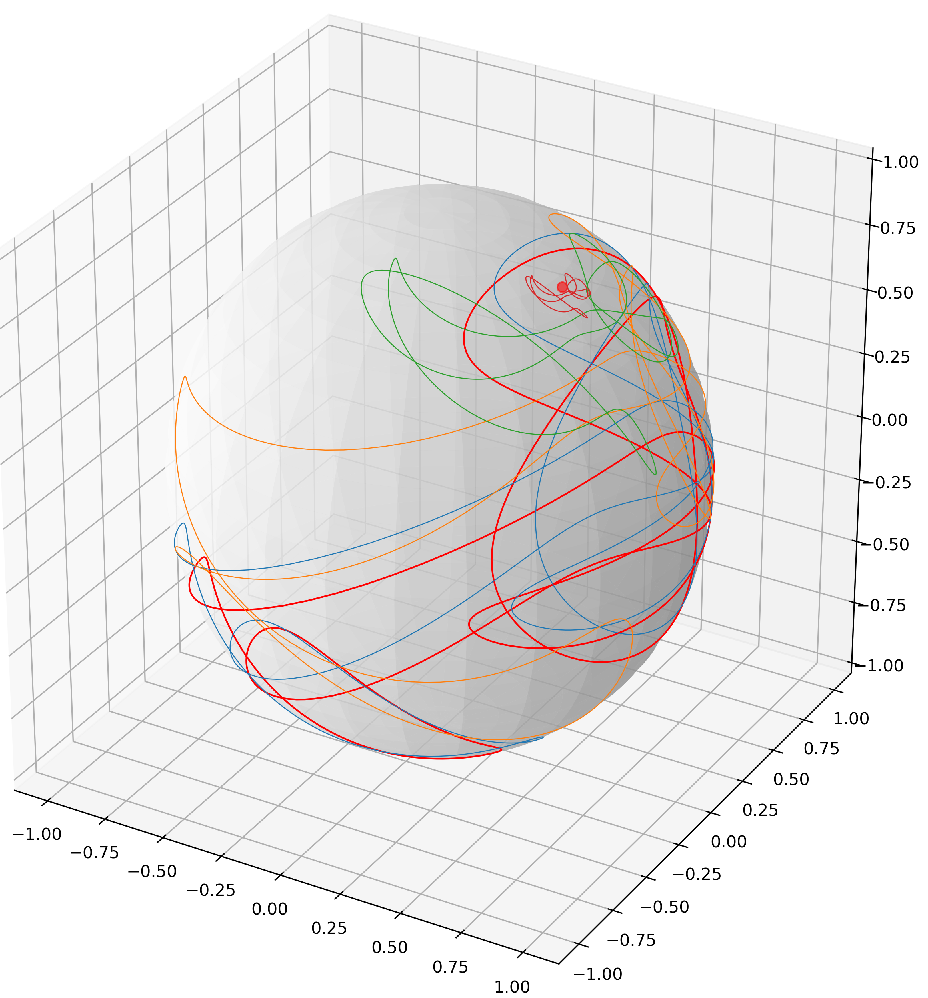
We formalize the phrase “local interpretation of Figure 1”.

Definition 7 (Locally-Defined GDL Model).

Fix atlases $\{\phi_{\alpha},U_{\alpha}\}_{\alpha\in A}$ and $\{\rho_{\zeta},V_{\zeta}\}_{\zeta\in Z}$ of $\mathcal{X}$ and of $\mathcal{Y}$ , respectively, and a “Euclidean model class” $\emptyset\neq{\mathscr{F}}\subseteq C({{{\mathbb{R}}^{p}}},{{{\mathbb{R}}^{m}}})$ . A locally defined GDL model is a family $\{{\mathscr{F}}_{\alpha}\}_{\alpha\in A}$ of models ${\mathscr{F}}_{\alpha}\subseteq C\left(\phi_{\alpha}(U_{\alpha}),\mathcal{Y}\right)$ , each of which is defined via:

{\mathscr{F}}_{\alpha}\triangleq\left\{\rho_{\zeta}^{-1}\circ\hat{f}\circ\phi_{\alpha}:\,\hat{f}\in{\mathscr{F}},\,\zeta\in Z\right\}.

(2)

Theorem 8 (Only Null-homotopic Maps are Approximable by Locally-Defined GDLs).

Let $\mathcal{X}$ and $\mathcal{Y}$ be complete connected Riemannian manifolds of positive dimension, satisfying (2), and let $\{{\mathscr{F}}_{\alpha}\}_{\alpha\in A}$ be a locally-defined GDL model. For every $\alpha\in A$ and every compact $\emptyset\neq K\subseteq U_{\alpha}$ :

(i)

For every $\zeta\in Z$ and every $g\in C({{{\mathbb{R}}^{p}}},{{{\mathbb{R}}^{m}}})$ , the map $\rho^{-1}_{\zeta}\circ g\circ\phi_{\alpha}$ is well-defined and in $C(K,\mathcal{Y})$ ,

(ii)

If there exists $f\in C(K,\mathcal{Y})$ which is not null-homotopic then, there is an $\epsilon>0$ satisfying:

\underset{\underset{\zeta\in Z,\,\alpha\in A}{g\in C({{{\mathbb{R}}^{p}}},{{{\mathbb{R}}^{m}}})}}{\inf}\,\underset{z\in K}{\sup}\,d_{\mathcal{Y}}\left(\rho_{\zeta}^{-1}\circ g\circ\phi_{\alpha}(z),f(z)\right)\geq\epsilon.

Theorem 8 is a simple necessary condition for a map with non-Euclidean outputs to be globally approximable by feedforward networks. In particular, when the global geometry of $\mathcal{Y}$ differs too greatly from Euclidean space, then functions which are not globally approximable necessarily exist.

Theorem 9 (Locally-Defined GDL Models are not Uniform Universal Approximators).

Let $\mathcal{X}$ and $\mathcal{Y}$ be complete connected Riemannian manifolds, with $p\geq m$ , $\mathcal{Y}$ compact and orientable, $\mathcal{X}$ satisfies Assumption 2, and let $\{{\mathscr{F}}_{\alpha}\}_{\alpha\in A}$ be a locally-defined GDL model. Then, there exists $\alpha\in A$ , $\zeta\in Z$ , a compact $\emptyset\neq K\subseteq\mathcal{X}$ , $x\in K\subseteq U_{\alpha}$ , an $\epsilon>0$ , and an $f\in C(K,\mathcal{Y})$ such that:

(i)

Each $\hat{f}\in{\mathscr{F}}_{\alpha}$ is a well-defined function in $C(K,\mathcal{Y})$ ,
(ii)

$\sup_{z\in K}\,\inf_{\hat{f}\in{\mathscr{F}}_{\alpha}}\,d_{\mathcal{Y}}\left(\hat{f}(z),f(z)\right)\geq\epsilon.$

3.1.1 Discussion: Why Uniform Approximation Poorly Suited to GDL Problems

The necessary condition for universality identified in Lemma 4 causes a major obstruction to building universal approximators in $C(\mathcal{X},\mathcal{Y})$ . This is because, the model class ${\mathscr{F}}\subset C(\mathcal{X},\mathcal{Y})$ needs to exhaust all the homotopy types therein. However, verifying that this condition is met is at-least as difficult as computing the homotopy groups of the output space $\mathcal{Y}$ (see Fomenko and Fuchs 2016 for details), which has recently been shown in Čadek et al. 2014 and in Matousek 2013 to be an (at-least) NP-hard problem. Therefore, verifying the compatibility of any model class ${\mathscr{F}}\subset C(\mathcal{X},\mathcal{Y})$ with the geometry of $\mathcal{Y}$ is computationally infeasible.

In the simplified setting where one instead considers only locally defined GDL models, Theorem 9 guarantees that when $\mathcal{X}$ and $\mathcal{Y}$ are both compact and connected Riemannian manifolds of positive dimension then there are functions in $C(\mathcal{X},\mathcal{Y})$ which cannot approximate all functions in $C(\mathcal{X},\mathcal{Y})$ uniformly on arbitrarily large compact subsets of $\mathcal{X}$ . Thus, any locally-defined GLD model is faced with the following problem: either the conditions for Theorem 9 are met, and therefore, the model class is not universal, or it is computationally infeasible to verify if the model class is universal.

Therefore, uniform approximation on “uncontrolled compact subsets” (i.e. of arbitrarily large maximum diameter) of a function between general Riemannian manifolds is not a well-suited notion of “universal approximation” for geometric deep learning. However, as we will now show, all these obstructions vanish when the models are only required to approximate the target function on compact subsets of $\mathcal{X}$ with a certain maximum diameter.

We now introduce the notion of “controlled universal approximation” (i.e.: universal approximation on compact subsets with a specific bounded maximum diameter). Moreover, we find that our GDN models are universal in this sense. We show that controlled universal approximation coincides with uniform approximation on compact sets when $\mathcal{X}$ and $\mathcal{Y}$ are non-positively curved (e.g. Euclidean space). Therefore, this notion of universality strictly extends the familiar notion of Hornik 1991, Pinkus 1999b, and Kidger and Lyons 2020 to the non-Euclidean setting without any of the topological obstructions of the “naive” uniform approximation on compact sets notion of universality.

Remark 10 (Connection to Relative Forms of Uniform Convergence).

In the general case, where $\mathcal{X}$ or $\mathcal{Y}$ may have somewhere positive curvature (e.g. any compact Riemannian manifolds of positive dimension) our notion of “controlled universality approximation” is most similar to density in the relative uniform convergence topologies introduced in Arens and Dugundji 1951 and studied in McCoy and Ntantu 1988, Nokhrin and Osipov 2009, and in Bouchair and Kelaiaia 2014.

3.2 Controlled Universal Approximation

We also make use of the function sending any $x\in\mathcal{X}$ and any $K\in(0,\infty]$ to:

\delta(\mathcal{X},x,K)\triangleq\sup_{0<r<K}r\frac{\operatorname{Vol}_{\mathcal{X}}\left(B_{\mathcal{X}}(x,r)\right)}{\operatorname{Vol}_{\mathcal{X}}\left(B_{\mathcal{X}}(x,r)\right)+\operatorname{Vol}_{T_{x}(\mathcal{X})}\left(B_{T_{x}(\mathcal{X})}(0,2r)\right)};

note, that $\delta(\mathcal{Y},y,K)$ is defined analogously. Our analysis relies on the following function, mapping any $K\in{\mathbb{R}}$ to the extended-real number:

K^{\star}\triangleq\begin{cases}\frac{\pi}{4\sqrt{K}}&:K>0\\ \infty&:K\leq 0.\end{cases}

Our approximation results concern the following locally-defined GDL model.

Definition 11 (Geometric Deep Feedforward Networks).

Fix $\sigma\in C({\mathbb{R}})$ . A geometric deep feedforward network (GDN) from $\mathcal{X}$ to $\mathcal{Y}$ at $x\in\mathcal{X}$ with activation function $\sigma$ , is a function $\hat{f}\in C(B_{\mathcal{X}}(x,\operatorname{inj}_{\mathcal{X}}(x)),\mathcal{Y})$ with representation:

\hat{f}\triangleq\operatorname{Exp}_{\mathcal{Y},y}\circ g\circ\operatorname{Exp}_{\mathcal{X},x}^{-1},

for some $g\in\mathcal{NN}_{p,m}^{\sigma}$ and some $y\in\mathcal{Y}$ .

Theorem 12 (Controlled Universal Approximation).

Let $\mathcal{X}$ and $\mathcal{Y}$ be connected complete Riemannian manifolds satisfying Assumption 2, of respective dimensions $p$ and $m$ , suppose that $\mathcal{X}$ is compact, and let $\sigma$ be an activation function satisfying Assumption 1. For any continuous function $f:\mathcal{X}\rightarrow\mathcal{Y}$ , any $\epsilon>0$ , and any $x\in\mathcal{X}$ , if:

\delta<\min\left\{\operatorname{inj}_{\mathcal{X}}(x),\omega^{-1}\left(f,\operatorname{inj}_{\mathcal{Y}}(f(x))\right)\right\},

(3)

then the following hold:

(i)

Well-Definedness of GDN: For every $g\in\mathcal{NN}_{p,m,p+m+2}^{\sigma}$ the map $\hat{f}\triangleq\operatorname{Exp}_{\mathcal{Y},f(x)}\circ g\circ\operatorname{Exp}_{\mathcal{X},x}^{-1}$ is well-defined on $\overline{B_{\mathcal{X}}(x,\delta)}$ ,

(ii)

Controlled Universal Approximation: There is a GDN $\hat{f}$ as in (i) satisfying:

\sup_{\tilde{x}\in\overline{B_{\mathcal{X}}\left(x,\delta\right)}}\,d_{\mathcal{Y}}\left(f(\tilde{x}),\hat{f}(\tilde{x})\right)\leq\epsilon.

(iii)

GDN Complexity Estimate: The depth of $g$ is recorded in Table 1, and it depends on $\sigma$ ’s regularity.

Furthermore, the right-hand side of (3) is lower-bounded via:

\min\left\{\delta(\mathcal{X},x,k^{\star}_{\mathcal{X}}),\omega^{-1}\left(f,\delta(\mathcal{Y},f(x),k^{\star}_{\mathcal{Y}})\right)\right\}\leq\min\left\{\operatorname{inj}_{\mathcal{X}}(x),\omega^{-1}\left(f,\operatorname{inj}_{\mathcal{Y}}(f(x))\right)\right\}.

(4)

Regularity of $\sigma$	Order of Depth
$C^{\infty}({\mathbb{R}})$ + Non-polynomial	$O\left(\frac{m(2\delta)^{2p}}{\kappa_{2}^{2p}\left(\omega^{-1}\left(f,\frac{\epsilon\kappa_{1}}{(1+\frac{p}{4})m}\right)\right)^{2p}}\right)$
Non-affine polynomial³³ 3 We must allow for one extra neuron per layer.	$O\left(\frac{m(m+p)(2\delta)^{4p+2}}{\kappa_{2}^{4p+2}\left(\omega^{-1}\left(f,\frac{\epsilon\kappa_{1}}{(1+\frac{p}{4})m}\right)\right)^{4p+2}}\right)$
$C({\mathbb{R}})$ + Non-polynomial	$O\left(\frac{m(2\delta)^{2p}}{\kappa_{2}^{2p}\omega^{-1}\left(f,\frac{\epsilon\kappa_{1}}{2m(1+\frac{p}{4})}\right)^{2p}\left(\kappa_{2}\omega^{-1}\left(\sigma,\frac{\epsilon}{2Bm(2^{(2\delta)^{2}[\omega^{-1}(f,\frac{\epsilon\kappa_{1}}{2m(1+\frac{p}{4})})]^{-2}+1}-1)}\right)\right)}\right)$

Where $\kappa_{1},\kappa_{2}>$ depend only on the curvature of $\mathcal{X}$ at $x$ and of $\mathcal{Y}$ at $f(x)$ , respectively.

Table 1: Approximation rates for GDNs based on activation function

Theorem 12 guarantees that universal approximation by GDNs on compact subsets of general Riemannian manifolds whose size is “controlled by the right-hand side of (3)” is possible; even if Theorem 9 mandates it typically fails “globally”; i.e., for arbitrarily large compact subsets of $\mathcal{X}$ . Thus, the “radius” in (3) quantifies the gap between “local” and “global” universal approximation.

Definition 13 (Universality Radius).

Let $\mathcal{X}$ and $\mathcal{Y}$ be Riemannian manifolds, and let $f\in C(\mathcal{X},\mathcal{Y})$ . The universality radius of $f$ at any $x\in\mathcal{X}$ is defined to be the quantity:

\mathcal{U}_{f}(x)\triangleq\min\left\{\operatorname{inj}_{\mathcal{X}}(x),\omega^{-1}\left(f,\operatorname{inj}_{\mathcal{Y}}(f(x))\right)\right\}.

Remark 14 (Analogy: Taylor Expansions and Controlled Universal Approximation).

The universality radius of any $f\in C(\mathcal{X},\mathcal{Y})$ plays a similar role to the radius and interval of convergence of a smooth function in classical calculus on ${\mathbb{R}}$ . This is because, on the interval of convergence about any $x\in\mathcal{X}$ a smooth function $f\in C^{\infty}({\mathbb{R}},{\mathbb{R}})$ can be locally approximated to arbitrary precision by its Taylor series. Analogously, any $f\in C(\mathcal{X},\mathcal{Y})$ can be universally approximated by a GDN on $B_{\mathcal{X}}(x,\mathcal{U}_{f}(x))$ . In both cases, the radius depends on the point of the input space about which the approximation is performed and on the regularity of the function.

One may ask if there is a broad class of input/output spaces for which the obstruction of Theorem 9 vanishes. In such cases, the GDN architecture can be developed about any point of the input space with the confidence that the the lower-bound (4) is infinity.

3.2.1 Local-to-Global Universality for Cartan-Hadamard Manifolds

Our search for input or output spaces with generically infinite universality radii begins with the Cartan-Hadamard Theorem (see (Jost 2017, Corollary 6.9.1)) and Cartan-Hadamard manifolds. These are simply connected, complete Riemannian manifolds of everywhere non-positive sectional curvature. Three important examples in geometric deep learning are the Hyperbolic spaces, the manifold of non-degenerate Gaussian probability measures with the Fisher-Rao distance (from information geometry; see (Ay et al. 2017, Equation 3.22)), and the familiar Euclidean spaces.

For Cartan-Hadamard manifolds, we have the following “local-to-global” result. That is, the next result describes a broad range of situations in which controlled universal approximation coincides with density in the uniform convergence on compact sets topology on $C(\mathcal{X},\mathcal{Y})$ .

Corollary 15 (From Local to Global Universal Approximation).

If $\mathcal{X}$ and $\mathcal{Y}$ are
Cartan-Hadamard manifolds, then the following estimate holds:

\inf_{x\in\mathcal{X}}\inf_{f\in C(\mathcal{X},\mathcal{Y})}\,\mathcal{U}_{f}(x)=\infty.

3.3 Breaking the Curse of Dimensionality via Efficient Datasets

3.3.1 Discussion: Overview of Our Approach

Thus far, as in most universal approximation papers, the objective has been to approximate $f\in C(\mathcal{X},\mathcal{Y})$ on arbitrary compact subsets of $\mathcal{X}$ for which universal approximation is not obstructed by Theorem 9. Indeed, classical constructive approximation results found in DeVore and Lorentz 1993 guarantee that cursed approximation rates (as in Theorem 12) are unavoidable. This phenomenon can be equally seen in the simple Euclidean case where it is confirmed in Gühring et al. 2020b that the best possible approximation rates for feedforward networks with ReLU activation function are unavoidably exponential in the involved spatial dimensions and the approximation error. Thus, the universal approximation problem is “cursed from the start” since we looked for a general rate which applies to any uniformly continuous function on any compact subset of the input space.

As pioneered in the quantitative approximation theorem of Barron 1993, the author found that the curse of dimensionality can be avoided if restrictions are placed on the set of functions which are considered for approximated. Since then, several other authors; e.g. Barron 1993, Yarotsky and Zhevnerchuk 2020, Siegel and Xu 2020, Gühring et al. 2020a, Suzuki 2019, and Cheridito et al. 2021, have identified sub classes of function which can be approximated by DNNs whose number of parameters does not depend adversely on the dimension of the input and output spaces⁴⁴ 4 These approximation results are not all in $C({{{\mathbb{R}}^{p}}},{{{\mathbb{R}}^{m}}})$ for the uniform distance; nevertheless, they all have the commonality of avoiding the curse of dimensionality by restricting the class of approximated functions within some larger function space in which the DNNs are dense. (potentially in different function spaces). We highlight that, each of these results takes a “functioncentric perspective” in that they focus on the impact of $f$ ’s regularity on the neural network approximation rates and omit the impact of the dataset on these approximation rates.

Here, we instead consider a “datacentric perspective” wherein we ask: given an $f:\mathcal{X}\rightarrow\mathcal{Y}$ , on which datasets⁵⁵ 5 Note a dataset need not be a training dataset but rather refers to the set on which we expect our approximation to hold. $\mathbb{X}$ (i.e.: non-empty subsets of $\mathcal{X}$ ) can $f$ be uniformly approximated by a GDN whose number of parameters does not depend adversely on the dimension of $\mathcal{X}$ and of $\mathcal{Y}$ ? Such datasets will be called efficient for $f$ . We will see that, if $f$ is sufficiently smooth then any dataset $\mathbb{X}$ is efficient for $f$ and, conversely, every “real-world dataset” (i.e. finite and non-empty) $\mathbb{X}$ is efficient for any (potentially discontinuous) function $f:\mathcal{X}\rightarrow\mathcal{Y}$ .

Remark 16 (Implications in the Euclidean Case).

In particular, as developed further in Section 4.5, our result strictly extend the dimension-free rates for DNNs in $C([0,1]^{p},{\mathbb{R}})$ obtained recently in Yarotsky and Zhevnerchuk 2020. Hence, even in the Euclidean case, our datacentric perspective is both novel and more general than the functioncentric perspective.

The idea of our approach is concisely summarized by Figure 4 wherein see that the green function $F$ coincides with the target function $f$ on the dataset $\mathbb{X}$ but $F$ is much more regular. Thus, if we instead approximate the more regular function $F$ by a GDN on all of the input space, then we can do so with a GDN which avoids the curse of dimensionality and simultaneously obtain an equally accurate approximation of target function $f$ on dataset $\mathbb{X}$ since both target function $f$ and the green function $F$ coincide thereon. Note that, our next main results does not assume that $\mathbb{X}$ is finite.

To formalize our task, we need to define what we mean by $F$ being “regular enough”. We consider an extension of the notion of regularity studied in Yarotsky and Zhevnerchuk 2020 but in the Riemannian context. Following Jost 2017, we make the following definition. We say that a function $f\in\bar{C}(\mathcal{X},\mathcal{Y})$ is regular if it has many higher-order partial derivatives, and if the last one of which locally distorts distance up to a linear scaling factor.

Definition 17 ( $C^{k,1}_{loc}(\mathcal{X},\mathcal{Y})$ ).

Fix a $k\in{\mathbb{N}}_{+}$ , and fix smooth atlases $(\phi_{\alpha},U_{\alpha})_{\alpha\in A}$ and $(\psi_{\zeta},V_{\zeta})_{\zeta\in Z}$ of $\mathcal{X}$ and of $\mathcal{Y}$ respectively. We say that $f\in\bar{C}(\mathcal{X},\mathcal{Y})$ belongs to $C^{k,1}_{\operatorname{loc}}(\mathcal{X},\mathcal{Y})$ if, for every $\alpha\in A$ and every non-empty compact subset $K\subseteq\phi_{\alpha}(U_{\alpha})$ we have:

\max_{\beta:|\beta|\leq k}\max_{x\in K}\,\|D^{\beta}\pi_{i}\circ\phi_{\alpha}\circ f\circ\psi_{\zeta}^{-1}(x)\|+\sup_{x,y\in K,\,x\neq y}\,\frac{\|D^{\beta}\pi_{i}\circ\phi_{\alpha}\circ f\circ\psi_{\zeta}^{-1}(x)-D^{\beta}\pi_{i}\circ\phi_{\alpha}\circ f\circ\psi_{\zeta}^{-1}(y)\|}{d_{Y}(x,y)}<\infty;

whenever the composition $\phi_{\alpha}\circ f\circ\psi^{-1}_{\zeta}$ is well-defined and where $\pi_{i}:{{{\mathbb{R}}^{m}}}\ni x\mapsto x_{i}\in{\mathbb{R}}$ is the canonical projection onto the $i^{th}$ -coordinate, $D^{\beta}=\frac{\partial^{|\beta|}}{\partial x_{\beta_{1}}\dots\partial x_{\beta_{|\beta|}}}$ , and $|\beta|$ is the length of the multi-index $\beta$ .

Therefore, our approach will be the following: replace the target function $f$ in $\mathbb{X}$ by a sufficiently smooth $F:\mathcal{X}\rightarrow\mathcal{Y}$ . Here, sufficiently smooth means that $F$ admits all $k$ continuous partial derivatives for some integer $k$ divisible by the dimension $p$ of $\mathcal{X}$ ; that is $F\in C^{k,1}_{\operatorname{loc}}(\mathcal{X},\mathcal{Y})$ and $k=np$ for some positive integer $n$ . In this case, we may approximate $F$ by a GDN depending on few parameters over a “regular” subset of $\mathcal{X}$ containing $\mathbb{X}$ and then restrict our approximation of $F$ to $\mathbb{X}$ thereby efficiently approximating $f$ . In what follows, we will denote the cardinality of a dataset $\mathbb{X}$ by $\#\mathbb{X}$ .

Remark 18 (The roles of $k$ and of $n$ ).

Suppose that $\mathbb{X}$ is finite. If $n$ equals to the number of points in $\mathbb{X}$ (i.e. if $n=\#\mathbb{X}$ ) then we would be seeking a function $F\in C_{\operatorname{loc}}^{np,1}(\mathcal{X},\mathcal{Y})$ satisfying

\displaystyle F(x)

\displaystyle=f(x)

\displaystyle\mbox{(for all }x\in\mathbb{X}).

(5)

Under the conditions that $k=\#\mathbb{X}p$ , the “smoothness” of $f$ ’s extension $F$ on the dataset $\mathbb{X}$ is effectively coupled with the dimension $p$ of $\mathcal{X}$ but it is also coupled to the number of datapoints in $\mathbb{X}$ . In this case, our next result (Theorem 24) implies that for any $\epsilon>0$ , $f$ can be approximated to $\epsilon$ -precision on $\mathbb{X}$ by a GDN determined by $\mathscr{O}\big(m(m^{2}-1)\epsilon^{-2p/3(np+1)}\big)$ trainable parameters.

However, the requirement that $k=\#\mathbb{X}p$ places a heavy restriction on the candidate smooth functions $F$ which could satisfying (5), since the condition $k=\#\mathbb{X}p$ necessitates that $F$ must be very smooth whenever $\#\mathbb{X}$ is large. A fortiori, this formulation is meaningless for any infinite $\mathbb{X}$ .

In fact, for our efficient approximation result (Theorem 24) to hold we do not need that $k=\#\mathbb{X}p$ ; rather, we only that $F\in C_{\operatorname{loc}}^{k,1}(\mathcal{X},\mathcal{Y})$ where $k$ is some positive integer divisible by $p$ . Therefore, by prespecifying some positive integer ( $n$ ) such that $k=np$ and looking for an $F\in C_{\operatorname{loc}}^{k,1}(\mathcal{X},\mathcal{Y})$ satisfying (5) we may still conclude that $f$ can be approximated on $\mathbb{X}$ to $\epsilon$ -precision by a GDN determined by $\mathscr{O}\big(m(m^{2}-1)\epsilon^{-2p/3(np+1)}\big)$ parameters. Moreover, by decoupling $k$ from the cardinality of $\mathbb{X}$ in this way, we no longer constrain the collection of “candidate functions” $F$ satisfying (5) for large (but finite) dataset $\mathbb{X}$ . Furthermore, by decoupling $k$ from $\#\mathbb{X}$ we can also meaningfully handle the case where $\mathbb{X}$ is infinite.

When this is possible, we show that the geometric arguments of Theorem 12 may be combined with an extension of the recently efficient approximation results of Yarotsky and Zhevnerchuk 2020 (describing efficient approximation of functions in $C^{np,1}_{\operatorname{loc}}({{{\mathbb{R}}^{p}}},{\mathbb{R}})$ by models in $\mathcal{NN}_{p,1}^{ReLU}$ ; where, $ReLU:x\to\max\{0,x\}$ ) to obtain an efficient approximating of $f$ by GDNs. The problem of replacing a function $f$ by a $C^{np,1}_{\operatorname{loc}}(\mathcal{X},\mathcal{Y})$ function coinciding with it on $\mathbb{X}$ is equivalent to the problem of extending $f$ on $\mathbb{X}$ to such a function. This latter problem is known as the Whitney Extension Problem, and dates back to Whitney 1934⁶⁶ 6 We require Fefferman 2005’s Extension Theorem since we are interested in uniform-type approximation results. If one were interested in applying our approach to other notions of approximation, e.g. Sobolev, or Besov norms, then the recent development surrounding extension theorems; see Fefferman et al. 2014, Heikkinen et al. 2016, Ambrosio and Puglisi 2020, or Bruè et al. 2021, would likely be equally central to obtaining “datacentric” uncursed rates by GDNs (or even classical DNNs) in those contexts. . Fortunately, this long-standing open problem has recently been solved in a series of papers: Bierstone et al. 2003, Fefferman 2005, and Bierstone et al. 2006. We leverage these analytic results to solve our efficient universal approximation problem⁷⁷ 7 A proper treatment of the Whitney Extension Problem is not aligned with our paper’s length target. The interested reader is referred to: Brudnyi and Brudnyi 2012a; Brudnyi and Brudnyi 2012b. .

3.3.2 Efficient Datasets

Our analysis begins by reformulating the conditions of Fefferman 2005’s Whitney Extension Theorem to suit our controlled universal approximation context. The best known conditions, to the authors’ knowledge, are (in the language of our context) the following.

Definition 19 (Efficient Datasets).

Fix $n\in{\mathbb{N}}_{+}$ , an $f:\mathcal{X}\rightarrow\mathcal{Y}$ , a dataset $\mathbb{X}$ , and set:

\ln(C^{\star})\triangleq\min\{\ln(\#\mathbb{X}),{2^{C}}\ln(C+1)\}\mbox{ and }C\triangleq{\binom{p+np}{p}}.

Then, $\mathbb{X}$ is $n$ -efficient for $f$ at $x\in\mathcal{X}$ if the following holds: for each $\{x_{c}\}_{c=1}^{C^{\star}}\subseteq\mathbb{X}$ there exists an $M>0$ , independent of $\{x_{c}\}_{c=1}^{C^{\star}}$ , and polynomials $p_{c}\in C({{{\mathbb{R}}^{p}}},{{{\mathbb{R}}^{m}}})$ of degree $np$ satisfying:

(i)

$p_{c}(\operatorname{Exp}_{\mathcal{X},x}^{-1}(x_{c}))=\operatorname{Exp}_{\mathcal{Y},f(x)}^{-1}(f(x_{c}))$ , for all $c=1,\dots,C^{\star}$
(ii)

$|\partial^{\beta}p_{c}(\operatorname{Exp}_{\mathcal{X},x}^{-1}(x_{c}))_{i}|\leq M$ , for all $c=1,\dots,K$ , $|\beta|\leq np$ , and $i=1,\dots,p$ ,
(iii)

$|\partial^{\beta}(p_{c}-p_{j})(\operatorname{Exp}_{\mathcal{X},x}^{-1}(x_{c}))_{i}|\leq M\left\|\operatorname{Exp}_{\mathcal{X},x}^{-1}(x_{c}))-\operatorname{Exp}_{\mathcal{X},x}^{-1}(x_{j}))\right\|^{nd-|\beta|}$ , for all $c,j=1,\dots,C^{\star}$ , $|\beta|\leq np$ , and $i=1,\dots,p$ ,

where $p_{c}(z)_{i}$ denotes the projection of $p_{c}$ onto its $i^{th}$ coordinate evaluated at $z$ . We say that $\mathbb{X}$ is $n$ -efficient for $f$ if it is $n$ -efficient for $f$ at each $x\in\mathcal{X}$ .

We begin by showing that functions for which all datasets are efficient extend the class of efficiently approximable functions of Yarotsky and Zhevnerchuk 2020 to the general Riemannian case.

Proposition 20 (Every Dataset is Efficient for $C^{np,1}_{\operatorname{loc}}(\mathcal{X},\mathcal{Y})$ -Functions).

Fix $f\in C^{np,1}_{\operatorname{loc}}(\mathcal{X},\mathcal{Y})$ and let $\mathbb{X}$ be a dataset satisfying the following: there is an $0\leq\eta<1$ and a $x\in\mathcal{X}$ such that:

\mathbb{X}\subseteq B_{\mathcal{X}}(x,\eta\operatorname{inj}_{\mathcal{X}}(x))\qquad\mbox{and}\qquad f(\mathbb{X})\subseteq B_{\mathcal{Y}}(f(x),\eta\operatorname{inj}_{\mathcal{Y}}(f(x)));

(6)

then, $\mathbb{X}\subseteq\mathcal{X}$ is $n$ -efficient for $f$ . In particular, condition (6) always holds if both $\mathcal{X}$ and $\mathcal{Y}$ are Cartan-Hadamard manifolds.

Proposition 20 is doubly insightful since it implies that functions for which every dataset is efficient are typical, from the approximation-theoretic standpoint.

Corollary 21 (Functions for Which Every Dataset is Efficient are Generic).

Consider the setting of Proposition 20. Let $C^{eff}(\mathcal{X},\mathcal{Y})$ denote the set of all $f\in\bar{C}(\mathcal{X},\mathcal{Y})$ with the following property: for every $x\in\mathcal{X}$ , each $0\leq\eta<1$ , and every finite $\mathbb{X}\subseteq B_{\mathcal{X}}(x,\eta\mathcal{U}_{f}(x))$ , there is some positive integer $n$ for which $\mathbb{X}$ is $n$ -efficient for $f$ . Then, the set $C^{eff}(\mathcal{X},\mathcal{Y})$ is dense in $\bar{C}(\mathcal{X},\mathcal{Y})$ .

Conversely, datasets for which every function is “efficient” are also prevalent. In fact, every “real-world dataset” (i.e. a non-empty finite dataset) has this property.

Proposition 22 (Real-World Datasets are Efficient for Any Function).

Let $\mathbb{X}$ be a finite set and $f:\mathcal{X}\rightarrow\mathcal{Y}$ . Suppose that $\mathbb{X}\subset B_{\mathcal{X}}(x,\eta\mathcal{U}_{f}(x))$ , for some $x\in\mathcal{X}$ and some $0<\eta<1$ . Assume that $\#\mathbb{X}<p$ and that $p$ divides $\#\mathbb{X}-1$ . Then $\mathbb{X}$ is $\frac{\#\mathbb{X}-1}{p}$ -efficient for $f$ .

Together, Propositions 20 and 22 show that efficient datasets describe a rich host of situations which are well beyond the scope of the classical perspective of assuming additional regularity of $f$ . To ensure a consistent narrative with the recent developments in Gühring et al. 2020b, Yarotsky 2017, and Yarotsky and Zhevnerchuk 2020, we focus on normalized datasets.

Assumption 3 (Normalizable Dataset).

Let $\mathbb{X}\subseteq\mathcal{X}$ be a dataset and $f:\mathcal{X}\rightarrow\mathcal{Y}$ . Then, $\mathbb{X}$ is $f$ -normalizable if there is some $x\in\mathcal{X}$ and some $0<\eta<1$ such that $\mathbb{X}\subset B_{\mathcal{X}}(x,\eta\,\mathcal{U}_{f}(x))$ and

\text{Exp}_{\mathcal{X},x}^{-1}(\mathbb{X})\subset[0,1]^{p};

(7)

Example 23 (Normalizability in the Euclidean Setting).

If $\mathcal{X}={{{\mathbb{R}}^{p}}}$ and $\mathcal{Y}={{{\mathbb{R}}^{m}}}$ then, $\mathcal{U}_{f}(x)=\infty$ and $\text{Exp}_{{{{\mathbb{R}}^{p}}},x}(y)=y+x$ ; thus, condition (7) reduces to $\{z-x\}_{z\in\mathbb{X}}\subseteq[0,1]^{p}.$

3.3.3 Breaking the Curse of Dimensionality on Efficient Datasets

Our result focuses on piecewise linear activation functions. By a piecewise linear activation function, we mean a $\sigma\in C({\mathbb{R}})$ for which there exists $B\in{\mathbb{N}}$ and distinct $x_{1},\dots,x_{B}\in{\mathbb{R}}$ satisfying: every $x\in{\mathbb{R}}-\{x_{b}\}_{b=1}^{B}$ is contained in an open interval in which $\sigma$ is linear and there is no such interval for each $x_{b}$ (for $b=1,\dots,B$ ). Note, if $\sigma$ is piecewise linear and non-affine then $B\geq 1$ . These include the ReLU activation function of Fukushima 1969, the leaky-ReLU activation function of Maas et al. 2013, the pReLU activation function of He et al. 2015, commonly implemented piecewise linear approximations to the Heavyside function (implemented for example in Abadi et al. 2015 and in Team et al. 2016), and many others.

Let $g\in\mathcal{NN}_{p,m}^{\sigma}$ have representation $g=W_{J}\circ\sigma\bullet\dots\circ\sigma\bullet W_{1}$ and $W_{j}(x)\triangleq A_{j}x+b_{j}$ (where $A_{j}$ is a $p_{j+1}\times p_{j}$ matrix, $b_{j}\in\mathbb{R}^{p_{j}}$ , $p_{1}=p$ , and $p_{J}=m$ ) for some $J\in{\mathbb{N}}_{+}$ with $J>1$ . Following Cheridito et al. 2021, the total number of trainable parameters in this representation of $g$ is defined by:

\sum_{j=1}^{J}p_{j}(p_{j-1}+1).

Theorem 24 (Polynomial Approximation Rates On Efficient Datasets).

Fix $n\in{\mathbb{N}}_{+}$ , let $f:\mathcal{X}\to\mathcal{Y}$ , $\sigma$ be a non-affine piecewise linear activation function, and let $\mathbb{X}$ be an $f$ -normalizable and $n$ -efficient dataset for $f$ . Then, for each $\epsilon>0$ , there is a $W\in{\mathbb{N}}_{+}$ , a $g\in\mathcal{NN}_{p,m:W}^{\sigma}$ , and a constant $\kappa>0$ (not depending on $\epsilon$ , $p$ , or on $m$ ), such that the GDN: $\hat{f}\triangleq\operatorname{Exp}_{\mathcal{Y},f(x)}\circ g\circ\operatorname{Exp}_{\mathcal{X},x}^{-1},$ satisfies the uniform estimate:

\sup_{x\in\mathbb{X}}\,d_{\mathcal{Y}}\left(f(x),\hat{f}(x)\right)\leq\kappa m^{\frac{1}{2}}\epsilon.

(8)

Moreover, $g$ satisfies the following sub-exponential complexity estimates:

(i)

Width: satisfies $m\leq W\leq m(4p+10)$ ,
(ii)

Depth: of order $\mathscr{O}\left(m+m\epsilon^{\frac{2p}{3(np+1)}-\frac{p}{np+1}}\right)$ ,
(iii)

Number of trainable parameters: is of order $\mathscr{O}\left(m(m^{2}-1)\epsilon^{-\frac{2p}{3(np+1)}}\right).$

Remark 25 (Dimension-Free Rates).

If $\mathbb{X}$ is $1$ -efficient for $f$ , then the network $g$ of Theorem 24 has depth roughly of the order $\mathscr{O}\left(m+m\epsilon^{\frac{-1}{3}}\right)$ and it depends on $\approx\mathscr{O}\left(m^{2}\epsilon^{-\frac{2}{3}}\right)$ trainable parameters.

Remark 26 (Discussion: Efficiency Datasets Vs. Target Functions Regularity).

An advantage of our efficient dataset approach to “non-cursed” approximation rates over the classical approach, which imposes regularity assumptions on the target function, is a practical one. Namely, given any dataset $\mathbb{X}$ , the Definition 19 can directly be verified. However, any additionally assumed regularity of the target function typically cannot be verified in practice.

3.4 Applications

We illustrate our theoretical framework developed thus far by establishing the universality of many commonly deployed geometric deep learning models.

3.4.1 Hyperbolic Feedforward Networks are Universal

Hyperbolic spaces have gained significant recent interest, in geometric deep learning, for their ability to represent complex tree-like structures much more efficiently and faithfully than Euclidean representations. Examples of such state-of-the-art embeddings include low-dimension representations of complex hierarchical datasets used in Nickel and Kiela 2017, efficient representations of complex social networks in Krioukov et al. 2010, tractable representations of large undirected graphs in Munzner 1997, and accurate representations of trees in Sala et al. 2018. Accordingly, the hyperbolic feedforward networks of Ganea et al. 2018, and Shimizu et al. 2021 have gained significant recent interest due to their ability to process such representations since they have inputs and outputs in (generalized) hyperbolic spaces. Let us briefly recall these notions before establishing the relevant quantitative universal approximation guarantees.

The (generalized) hyperbolic spaces $\mathbb{D}^{n}_{c}$ is the Cartan-Hadamard manifold $\{x\in{{{\mathbb{R}}^{n}}}:\,c\|x\|^{2}<1\}$ whose Riemannian structure induces the distance function:

d_{c}(x,y)\triangleq\frac{2}{\sqrt{c}}\tanh^{-1}\left(\sqrt{c}\left\|\frac{(1-c\|x\|^{2})y-(1-2cx^{\top}y+c\|y\|^{2})}{1-2cx^{\top}y+c^{2}\|x\|^{2}\|y\|^{2}}\right\|\right).

The hyperbolic feedforward networks of Ganea et al. 2018 are defined via a series of complicated operations; however, as the authors later note (Ganea et al. 2018, Equation (26)) every hyperbolic feedforward network $\hat{f}:\mathbb{D}^{p}_{c}\rightarrow\mathbb{D}^{m}_{c}$ can equivalently be represented by:

\hat{f}=\operatorname{Exp}_{\mathbb{D}^{p}_{c},0}\circ f\circ\operatorname{Exp}_{\mathbb{D}^{m}_{c},0}^{-1},

(9)

where $f\in\mathcal{NN}_{p,m}^{\sigma}$ . We note that closed-form expressions for $\operatorname{Exp}_{\mathbb{D}^{m}_{c},0}$ and $\operatorname{Exp}_{\mathbb{D}^{m}_{c},0}^{-1}$ are known (see (Ganea et al. 2018, Lemma 2)). Our framework therefore implies the following universal approximation theorem for hyperbolic feedforward networks, which is a quantitative version of (Kratsios and Bilokopytov 2020, Corollary 3.16).

Corollary 27 (Hyperbolic Neural Networks are Universal Approximators).

Let $\sigma\in C({\mathbb{R}})$ satisfy the Kidger-Lyons conditions. Fix $c,\epsilon>0$ , $f\in C(\mathbb{D}^{p}_{c},\mathbb{D}^{m}_{c})$ , and a non-empty compact subset $K\subseteq\mathbb{D}^{p}_{c}$ . Then, there exists a hyperbolic feedforward network $\hat{f}$ satisfying:

\sup_{x\in K}\,d_{c}(f(x),\hat{f}(x))<\epsilon,

(10)

of width $m+p+2$ and whose depth is recorded in Table 1.

We also substantially sharpened the variant of the above rates when the training and testing data belong to an $f$ -normalizable and $n$ -efficient dataset.

Corollary 28 (Hyperbolic Neural Networks are Efficient Universal Approximators).

Consider the setting of Corollary 27 and let $n\in{\mathbb{N}}_{+}$ , $\sigma$ be a non-affine piecewise linear activation function, and let $\mathbb{X}$ be an $f$ -normalizable and $n$ -efficient dataset for $f$ . Then, there is a $W\in{\mathbb{N}}_{+}$ , a $g\in\mathcal{NN}_{p,m:W}^{\sigma}$ , and a constant $\kappa>0$ not depending on $\epsilon$ , $p$ , or on $m$ , such that the hyperbolic feedforward network: $\hat{f}\triangleq\operatorname{Exp}_{\mathbb{D}^{m}_{c},f(0)}\circ g\circ\text{Exp}_{\mathbb{D}^{p}_{c},0}^{-1},$ satisfies the approximation bound:

\sup_{x\in\mathbb{X}}d_{c}\left(f(x),\hat{f}(x)\right)<\kappa\sqrt{m}\epsilon.

Furthermore, the DNN $g$ satisfies the sub-exponential complexity estimates:

(i)

Width: satisfies $m\leq W\leq m(4p+10)$ ,
(ii)

Depth: of order $\mathscr{O}\left(m+m\epsilon^{\frac{2p}{3(np+1)}-\frac{p}{np+1}}\right)$ ,
(iii)

Number of trainable parameters: is of order $\mathscr{O}\left(m(m^{2}-1)\epsilon^{-\frac{2p}{3(np+1)}}\right).$

3.4.2 Universal Symmetric Positive-Definite Matrix-Valued Networks

Non-degenerate covariance matrices are fundamental tools for describing the non-trivial interdependence of various stochastic phenomena; with notable applications ranging from mathematical finance (Markowitz 1991) to computer vision (see Haralick 1996). Briefly, any covariance matrix $A$ between $p$ different random variables $\xi_{1},\dots,\xi_{p}$ can be identified (component-wise) with a $p\times p$ vector in the low-dimensional subset $P_{p}^{+}\subset{{\mathbb{R}}^{p\times p}}$ given by:

P_{p}^{+}\triangleq\left\{A\in{{\mathbb{R}}^{p\times p}}:\,(\forall x\in{{{\mathbb{R}}^{p}}}-\{0\})\,x^{\top}Ax>0\right\};

here, we have identified $p\times p$ -matrices with vectors in $p^{2}$ via $(A_{i,j})_{i,j=1}^{p}\mapsto(A_{1,1},\dots,A_{p,1},\dots,A_{p,p})$ . In fact, $P_{p}^{+}$ is a (non-linear) differentiable submanifold of ${{\mathbb{R}}^{p\times p}}$ (see Pennec et al. 2006).

The Euclidean metric $P_{p}^{+}$ is not well-suited to the description of covariance matrices. For example, suppose that $\xi=(\xi_{1},\dots,\xi_{p})$ and $\zeta=(\zeta_{1},\dots,\zeta_{p})$ are vectors of features from some dataset of images. One would expect that, since the content of any image does not change if the image is rotated or shifted, then the relation between the covariance matrices $\text{Cov}(\xi)$ and $\text{Cov}(\zeta)$ should be equal to the distance of $\text{Cov}(X\xi+b)=X^{\top}\text{Cov}(\xi)X$ and $\text{Cov}(X\zeta+b)=X^{\top}\text{Cov}(\zeta)X$ ; where $X$ is a $p\times p$ -orthogonal matrix and $b\in{{{\mathbb{R}}^{p}}}$ (since $x\mapsto Xx+b$ is exactly a rotation and shift in ${{{\mathbb{R}}^{p}}}$ ). However, this is not the case when comparing covariance matrices dissimilarity with the Euclidean distance.

In Pennec et al. 2006, a solution to this problem was obtained via the so-called “affine-invariant” metric. This distance function was obtained by equipping $P_{p}^{+}$ with a specific Cartan-Hadamard structure designed to encode invariances under the aforementioned symmetry. The distance function $d_{+}$ of this Riemannian metric satisfies $d_{+}(A,B)=d_{+}(X^{\top}AX,X^{\top}BX)$ for any $p\times p$ -orthogonal matrix $X$ and any $A,B\in P_{p}^{+}$ and $d_{+}$ is computed via:

d_{+}(A,B)\triangleq\left\|\sqrt{A}\log\left(\sqrt{A}^{-1}B\sqrt{A}^{-1}\right)\sqrt{A}\right\|_{2};

where $\|\cdot\|_{2}$ is the Fröbenius norm on ${{\mathbb{R}}^{p\times p}}$ , $\log(\cdot)$ is the inverse of the matrix exponential $\exp(\cdot)$ and $\sqrt{\cdot}$ is the matrix square-root (both of which are well-defined on $P_{p}^{+}$ ). The Riemannian exponential maps is obtained as follows. Identify ${{\mathbb{R}}^{p(p+1)/2}}$ with the set of $\text{Sym}_{p}$ of $p\times p$ -symmetric-matrices:

Sym_{p}:\,{{\mathbb{R}}^{p(p+1)/2}}\ni(a_{1,1},\dots,a_{1,p},\dots,a_{p,p})\mapsto\begin{pmatrix}a_{1,1}&\dots&a_{1,p}\\ \vdots&\ddots&\vdots\\ a_{1,p}&\dots&a_{p,p}\end{pmatrix}\in\text{Sym}_{p}.

(11)

Under this identification, the Riemannian exponential map and its inverse are computed to be:

	$\displaystyle\text{Exp}_{P_{p}^{+},A}(B)$	$\displaystyle=\sqrt{A}\exp\left(\sqrt{A}^{-1}Sym_{p}(B)\sqrt{A}^{-1}\right)\sqrt{A}$		(12)
	$\displaystyle\text{Exp}_{P_{p}^{+},A}(B)^{-1}$	$\displaystyle=Sym_{p}^{-1}[\sqrt{A}\log\left(\sqrt{A}^{-1}B\sqrt{A}^{-1}\right)\sqrt{A}].$		(12)

The suitability of this geometry to the problem of covariance-matrix feature description is well-studied, especially in the computer vision literature. Most relevant to our program, in Meyer et al. 2011b the authors introduce a class of non-Euclidean regression models on $P_{p}^{+}$ and in Bonnabel 2013 and Bécigneul and Ganea 2018 classes of optimization algorithms were introduced which leverage the Riemannian geometry of $P_{p}^{+}$ . Likewise, there have been numerous optimization software advances specifically designed to handle such situations Boumal et al. 2014, Townsend et al. 2016, and Miolane et al. 2020.

Subsequently, Baes et al. 2019 and Herrera et al. 2020 extended some of these ideas by introducing geometric deep learning models with inputs and outputs from the set of $p\times p$ -symmetric positive semi-definite matrices to itself. Thereafter, in Kratsios and Bilokopytov 2020 the authors derived a universal extension of the regression model of Meyer et al. 2011b which necessarily inputs and outputs matrices from $P_{p}^{+}$ and $P_{m}^{+}$ , respectively. The latter model class of “affine-invariant” GDNs have the representation:

\hat{f}\triangleq\text{Exp}_{P_{m}^{+},I_{m}}\circ g\circ\text{Exp}_{P_{p}^{+},I_{p}}^{-1}\in C(P_{p}^{+},P_{m}^{+});

(13)

where, $g\in\mathcal{NN}_{\frac{p(p+1)}{2},\frac{m(m+1)}{2}}^{\sigma}$ . The following are, respectively, quantitative and efficient improvements of the universal approximation theorems for the model class (13) derived in (Kratsios and Bilokopytov 2020, Section 3.2.1). We denote the set of $p\times p$ -orthogonal matrices by $O(p)$ .

Corollary 29 (Universality of the Affine-Invariant Networks of (13)).

Let $\sigma\in C({\mathbb{R}})$ satisfy the Kidger-Lyons conditions. Fix $\epsilon>0$ , $f\in C(P_{p}^{+},P_{m}^{+})$ , and a non-empty compact subset $K\subseteq P_{m}^{+}$ . Then, there exists an “affine-invariant” GDN $\hat{f}$ satisfying:

\max_{A\in K}\sup_{X\in O(p)}\,d_{+}\left(X^{\top}f(A)X,X^{\top}\hat{f}(A)X\right)<\epsilon.

(14)

Moreover, $g$ in the representation (13), has width at-most $\frac{p(p+1)+m(m+1)+4}{2}$ and its depth is recorded in Table 1 with $2^{-1}p(p-1)$ and $2^{-1}m(m-1)$ in place of $p$ and $m$ , respectively.

Using the concept of efficient dataset, we are able to refine the above theorem.

Corollary 30 (Affine-Invariant GDNs are Efficient Universal Approximators).

Consider the setting of Corollary 29 and let $n\in{\mathbb{N}}_{+}$ , $\sigma$ be a non-affine piecewise linear activation function, and let $\mathbb{X}$ be an $f$ -normalizable and $n$ -efficient dataset for $f$ . Then, there is a $W\in{\mathbb{N}}_{+}$ , a $g\in\mathcal{NN}_{2^{-1}p(p+1),2^{-1}m(m+1):W}^{\sigma}$ , and a constant $\kappa>0$ not depending on $\epsilon$ , $p$ , or on $m$ , such that the GDN $\hat{f}\triangleq\operatorname{Exp}_{P_{m}^{+},f(0)}\circ g\circ\operatorname{Exp}_{P_{p}^{+},0}^{-1},$ satisfies the approximation bound:

\sup_{x\in K}\sup_{X\in O_{,}}d_{+}\left(X^{\top}f(x)X,X^{\top}\hat{f}(x)X\right)<\frac{\kappa\sqrt{m(m+1)}}{\sqrt{2}}\epsilon.

Furthermore, $g$ satisfies the sub-exponential complexity estimates:

(i)

Width: satisfies $m\leq W\leq 2^{-1}m(m+1)(2p(p+1)+10)$ ,
(ii)

Depth: of order $\mathscr{O}\left(m(m+1)(1+\epsilon^{\frac{p(p+1)}{3(2^{-1}np(p+1)+1)}-\frac{p(p+1}{np(p+1)+2}})\right)$ ,
(iii)

Number of trainable parameters: of order $\mathscr{O}\left(m(m+1)((m(m+1))^{2}-1)\epsilon^{-\frac{2p(p+1)}{3(np^{2}+np+2)}}\right).$

3.4.3 Spherical Neural Networks and Approximation in Kendall’s Pre-Shape Space

Our last illustration focuses on Theorem 9. As described in Straub et al. 2015, spherical data plays a central role in many computer vision applications as a natural medium for describing direction data. This, and its connections to various other areas such as geo-statistics, has made learning from spherical data an active area of research both in the machine learning (see Dutordoir et al. 2020, and Hamsici and Martinez 2007), and in the statistics communities (see Dai and Müller 2018a).

Geodesics on the sphere are well-studied; for example, the distance on $S^{p}$ is $d_{S^{p}}(x,y)=\arccos{(y^{\top}x)}.$ Most importantly for our analysis, the Riemannian exponential map, and its inverse, at any $x\in S^{p}$ admits the following closed-form expressions

\operatorname{Exp}_{S^{p},x}(v)=\cos(\|v\|)x+\sin(\|v\|)\frac{v}{\|v\|}\mbox{ and }\operatorname{Exp}_{S^{p},x}(y)^{-1}=\frac{y-(y^{\top}x)x}{\|y-(y^{\top}x)x\|}\arccos{(y^{\top}x)},

(15)

(see (Dai and Müller 2018a, page 3341) for example). Unlike the geometries in the two previous examples, the sphere is positively curved, with sectional curvature always equal to $1$ . Consequentially the Riemannian Exponential map’s inverse, about any point $x\in S^{p}$ , is not globally defined.

Corollary 31 (Local Quantitative Deep Universal Approximation for Spherical Data).

Let $\sigma\in C({\mathbb{R}})$ satisfy Assumption 1. For any continuous function $f:S^{p}\rightarrow S^{m}$ , any $\epsilon>0$ , given any $B_{S^{p}}(x,\delta)\subseteq S^{p}$ for which $0<\delta<\pi$ then, for every $g\in\mathcal{NN}_{p,m,p+m+2}^{\sigma}$ the GDN $\hat{f}\triangleq\operatorname{Exp}_{S^{m},f(x)}\circ g\circ\operatorname{Exp}_{S^{p},x}^{-1},$ is well-defined on $\overline{B_{S^{p}}(x,\delta)}$ and there is one such $\hat{f}$ satisfying the approximation bound:

{\underset{x\in\overline{B_{S^{p}}\left(x,\delta\right)}}{\max}\,d_{S^{m}}\left(f(x),\hat{f}(x)\right)\leq\epsilon.}

Moreover, $g$ ’s depth is recorded in Table 1.

Remark 32.

The quantity $\pi$ estimating the maximum radius of the ball $B_{S^{p}}(x,\delta)$ in Corollary 31 is a lower-bound for $\mathcal{U}_{f}(x)$ . This estimate is specific to the sphere’s geometry, where we have tightened the generic estimate of (4) via Klingenberg 1968’s Quarter-Pinched Sphere Theorem.

The obstruction identified in Theorem 9 has the following consequence for spherical spaces.

Corollary 33 (Universal Approximation on Spheres is Local).

If $\mathcal{X}=\mathcal{Y}=S^{m}$ , then there exists a non-empty compact subset ${\mathscr{K}}\subseteq S^{m}$ , $x\in{\mathscr{K}}$ , $\epsilon>0$ , such that for every $k\in{\mathbb{N}}$ , and for every $g\in\mathcal{NN}_{m,m;k}^{\sigma}$ , the map $\operatorname{Exp}_{S^{m},f(x)}\circ g\circ\operatorname{Exp}_{S^{m},x}^{-1}$ is a well-defined function in $C({\mathscr{K}},\mathcal{Y})$ , but

{\underset{\underset{y\in S^{m},\,k\in{\mathbb{N}}_{+}}{g\in\mathcal{NN}_{m,m,k}^{\sigma}}}{\inf}\,\sup_{z\in{\mathscr{K}}}\,d_{\mathcal{Y}}\left(\operatorname{Exp}_{S^{m},f(x)}\circ g\circ\operatorname{Exp}_{S^{m},x}^{-1}(z),1_{S^{m}}(z)\right)\geq\epsilon.}\vskip 7.5pt

Remark 34 (Universal Approximation Theorem in Kendall’s Pre-Shape Space).

As
shown in Kendall 1984 and Le and Kendall 1993, high-dimensional spheres coincide with Kendall’s pre-shape space. Therefore, Corollary 33 guarantees that GDNs between Kendall’s pre-shape spaces are universal. These GDNs are a direct “deep learning” extension of the Procrustean (pre-shape space) regressors of Thomas Fletcher P. 2013.

4 Main Results on Building Universal GDL Models using GDNs

Next, we treat GDNs as elementary building blocks, and we derive several results which describe how to combine GDNs to build universal geometric deep learning models compatible with complicated geometries; summarized in Figure 5. This additional flexibility is gained by combining multiple GDNs using “geometric processing layers” (symbolized arrows in Figure 5 other than $\hat{f}_{i}$ ). These are non-trainable layers that encode specific geometric “features” into our geometric deep learning models, such as products, quotients, parameterization, or boundary-like regions.

Figure 5: The geometric deep learning model’s full computational graph.

We briefly outline Figure 5: $\phi$ is a feature map with the UAP-invariance property of Kratsios and Hyndman 2021, each of the $\hat{f}_{i}$ are GDNs mapping into “deep feature spaces $\mathcal{F}_{i}$ ”, the $\rho_{i}$ are “good” quotient maps which impose symmetries on the deep features in $\mathcal{F}_{i}$ , the green arrows are a parallelization of the architectures thus far via a “skip connection” (analogously to He et al. 2016 and Srivastava et al. 2015), and $\rho$ parameterizes the output space $\mathcal{Y}$ up to a “negligible subset of $\mathcal{Y}$ ” (where our notion of negotiability is similar to that of Toruńczyk 1978 and to van Mill 2001).

We progressively introduce each geometric processing layer in Figure 5 and incrementally derive its universal approximation theorem. Each step of our derivative will correspond to a geometric deep learning model defined by a computational sub-graph of Figure 5.

4.1 Feature Spaces and Quotient Layers: For Quotient Geometries

Often, a metric space $\mathcal{Y}$ ’s geometry is extremely complicated, but its description can substantially be simplified by understanding its points as equivalence classes of symmetries defined on a “simpler” $m$ -dimensional Riemannian manifold $\mathcal{F}$ . We consider the situation of Figure 6.

Figure 6: Factorizing the Target Function.

Our setting is formalized as follows. Let $G\subset C({\mathcal{F}},{\mathcal{F}})$ be a set of surjective isometries; that is, each $g\in G$ does not distort the relative distance between any two points $z_{1},z_{2}\in{\mathcal{F}}$ since $d_{{\mathcal{F}}}(z_{1},z_{2})=d_{{\mathcal{F}}}(g(z_{1}),g(z_{2}))$ . We require the isometries in $G$ to be “compatible” in the sense that:

Assumption 4 (Symmetric Space).

$1_{{\mathcal{F}}}\in G$ and if $g_{1},g_{2}\in G$ then⁸⁸ 8 We note that $g_{2}^{-1}$ is always well-defined since every isometry is injective; thus, $g_{2}$ is a bijection and therefore it has a unique two-sided inverse $g_{2}^{-1}$ . $g_{1}\circ g_{2}^{-1}\in G$ .

We consider output spaces $\mathcal{Y}$ which are “invariant/symmetric to the isometries in $G$ ”. Such $\mathcal{Y}$ are called symmetric spaces and are widely studied both in the context of density estimation when data and/or parameters lie in a low-dimensional manifold in Li et al. 2020, non-linear dimension reduction Fletcher et al. 2004, learning faithful graph representations in Lopez et al. 2021, stochastic filtering in Pontier and Szpirglas 1986, as well as several other instances in machine learning literature and its adjacent research areas.

Following (Burago et al. 2001, Section 3.3), we do this by setting (resp. identifying) the points in $\mathcal{Y}$ to be (resp. with) the equivalence classes: $[z]\triangleq\left\{z^{\prime}:\,(\exists g\in G)\,g(z)=z^{\prime}\right\}.$ By (Burago et al. 2001, Lemma 3.3.6), the set $\mathcal{Y}$ is made into a metric space since the map:

\bar{d}_{{\mathcal{F}}}([z_{1}],[z_{2}])=\inf_{g\in G}\,\bar{d}_{{\mathcal{F}}}(z_{1},g(z_{2})),

is a well-defined metric on $\mathcal{Y}$ . Note that, $\bar{d}_{{\mathcal{F}}}([z_{1}],[z_{2}])\leq d_{{\mathcal{F}}}(z_{1},z_{2})$ for any $z_{i}\in[z_{i}]$ and $i=1,2$ . We call $\bar{d}_{{\mathcal{F}}}$ the quotient metric on $\mathcal{Y}$ and $\mathcal{Y}$ the quotient metric space of ${\mathcal{F}}$ generated by the symmetries in $G$ . If ${\mathcal{F}}$ ’s geometry is compatible with the symmetries described by $G$ (Assumption 5 below), then the projection map:

\rho_{1}:\,{\mathcal{F}}\ni z\mapsto[z]\in\mathcal{Y},

(16)

implies that: “locally, ${\mathcal{F}}$ looks like a disjoint union of identical pieces of $\mathcal{Y}$ and that it looks the same everywhere”. Following (Burago et al. 2001, Proposition 3.4.15.)), this happens when:

Assumption 5 (Compatibility between $G$ and ${\mathcal{F}}$ ).

(i)

For each $z\in{\mathcal{F}}$ there is a $k_{z}>0$ such that if $d(z,g(z))<k_{z}$ then $g$ is the identity,
(ii)

For each $z\in{\mathcal{F}}$ and each $g\in G$ if $g\neq 1_{\mathcal{F}}$ then $z\neq g(z)$ .

Example 35 ((Hatcher 2002, Exercise 1.3.23)).

If $G$ is finite, then Assumption 5 (ii) holds.

The deep feature space must be connected by paths and every such path is topologically comparable.

Assumption 6 (The Deep Feature Space is Simply Connected).

The deep feature space ${\mathscr{F}}$ is connected and simply connected.

Example 36.

The Euclidean space ${{{\mathbb{R}}^{p}}}$ , the space of symmetric positive definite matrices, and the hyperbolic space each satisfy Assumption 6. Nevertheless, if $p\geq 1$ , then Examples 5 and 6 shows that $S^{p}$ is still much more complicated than ${{{\mathbb{R}}^{p}}}$ , topologically.

We arrive at the following quantitative non-Euclidean universal approximation theorem.

Theorem 37 (Universal Approximation for Quotient Metric Spaces).

Suppose that Assumptions 4 and 5 hold, and that Assumption 6 also holds for $\mathcal{X}$ and for ${\mathcal{F}}$ and let $\sigma\in C({\mathbb{R}})$ satisfy Assumption 1. Let $\epsilon>0$ , $x\in\mathcal{X}$ , $f\in C(\mathcal{X},\mathcal{Y})$ , $\mathbb{X}\subset B_{\mathcal{X}}(x,\mathcal{U}_{f}(x))$ be a compact dataset, and $\rho_{1}:\mathcal{F}\ni z\mapsto[z]\in\mathcal{Y}$ . There is a GDN $\hat{f}$ with representation: $\hat{f}=\text{Exp}_{\mathcal{F},f}\circ g\circ\text{Exp}_{\mathcal{X},x}^{-1},$ for some $y\in\mathcal{F}$ , where $g\in\mathcal{NN}_{p,m,W}^{\sigma}$ such that:

\sup_{x\in\mathbb{X}}\,\bar{d}_{{\mathcal{F}}}\left(f(x),\rho_{1}\circ\hat{f}(x)\right)<\epsilon.

(17)

Moreover, $W=p+m+2$ and $g$ ’s depth is as in Table 1.

Examples: Universal Approximators with computational Subgraph of Figure 6

The following example is an essential component of the projective shape space introduced by Mardia and Patrangenaru 2005. We return to the following manifold in Section 4.4.

Example 38 (Universal Approximators to the Real Projective Space ( ${\mathbb{R}}P^{m}$ )).

An element of the real projective space ${\mathbb{R}}P^{m}$ is a line in ${{\mathbb{R}}^{m+1}}$ passing through the origin. Since every such line is determined by its intersections with $S^{m}\triangleq\left\{x\in{{\mathbb{R}}^{m+1}}:\,\|x\|=1\right\}$ then elements of ${\mathbb{R}}P^{m}$ are:

[x]\triangleq\left\{\{x,-x\}:\,x\in S^{m}\right\};

where, $G=\{1_{S^{m}},[x\mapsto-x]\}$ . Furthermore, in (Hatcher 2002, Example 1.43), it is shown that $G$ and $S^{m}$ satisfy Assumptions 4 and 5. By Example 36, ${{{\mathbb{R}}^{p}}}$ and $S^{m}$ satisfy Assumption 6. Thus, the projection map $\rho_{1}:S^{m}\ni y\mapsto[y]\in{\mathbb{R}}P^{m}$ verified the conditions of Theorem 37 and ${\mathbb{R}}P^{m}$ is a quotient of $S^{m}$ by the symmetry defined by $G$ . Since Corollary 33 implies that deep neural models

\{\operatorname{Exp}_{S^{m},f(x)}\circ g:\,g\in\mathcal{NN}_{p,m}^{\sigma}\},

are locally universal in $C({{{\mathbb{R}}^{p}}},S^{m})$ , then Theorem 37 implies that each $f\in C({{{\mathbb{R}}^{p}}},{\mathbb{R}}P^{m})$ can be locally be approximated by a deep neural model of the form $\rho_{1}\circ\operatorname{Exp}_{S^{m},f(x)}\circ g.$

Our next illustration of Theorem 37 concerns universal approximators into the “flat torus”. Examples of the torus geometry in data visualization in Li 2004 and in Maron et al. 2017.

Example 39 (Universal Approximators on the Flat Torus ( $\mathbb{T}^{m}$ )).

Let $G$ be the “integer lattice translations”: $G\triangleq\left\{g:{{{\mathbb{R}}^{m}}}\ni z\mapsto z+k\in{{{\mathbb{R}}^{m}}}\right\}_{k\in{\mathbb{Z}}^{m}}.$ Then $G$ satisfies Assumption 4 and ${{{\mathbb{R}}^{m}}}$ satisfies Assumption 5. Example 36 states that ${{{\mathbb{R}}^{p}}}$ and ${{{\mathbb{R}}^{m}}}$ satisfy Assumption 6. The classes in $\mathcal{Y}$ are therefore in correspondence with points in the cube $[0,1]^{m}$ but the distance between any $y_{1},y_{2}\in\mathcal{Y}$ is the “flat toral distance”:

\bar{d}_{{{{\mathbb{R}}^{m}}}}(y_{1},y_{2})=\inf_{z\in{\mathbb{Z}}^{m}}\,\|y_{1}-(y_{2}+z)\|.

In this space, we are allowed to “teleport” along nodes in integer lattice ${\mathbb{Z}}^{m}$ but every other movement counts. It is a standard exercise to show that the above $G$ satisfies Assumptions 4 and Assumption 5. Thus, Theorem 37 implies that for every $f\in C({{{\mathbb{R}}^{p}}},\mathbb{T}^{m})$ there is a DNN $\hat{f}\in\mathcal{NN}_{p,m}^{\sigma}$ such that $\rho_{1}\circ\hat{f}$ locally approximates $f$ .

4.2 Skip Connections and Parallelization: For Product Geometries

In Gribonval Rémi et al. 2021, the authors describe a calculus for “parallelizing” several feedforward networks $g_{1},\dots,g_{I}\in C({{{\mathbb{R}}^{p}}},{\mathbb{R}})$ to efficiently form a deep neural model in $C({{{\mathbb{R}}^{p}}},{{\mathbb{R}}^{I}})$ . There, the parallelized model implements the map:

{{{\mathbb{R}}^{p}}}\ni x\mapsto(g_{1}(x),\dots,g_{I}(x))\in{{\mathbb{R}}^{I}}.

(18)

In Cheridito et al. 2021, the author gave conditions on the activation function $\sigma$ under which the map (18) could be implemented by a single feedforward network. Otherwise, the map of (18) are $I$ different learning models defined by a more complicated computational graph where the last layer can be understood as a sort of “skip connection”. Note that, most commonly used deep learning software such as, Abadi et al. 2015 and Team et al. 2016, are designed to handle these types of computational graphs.

Figure 7: Parallelized Computational Graph.

In the geometric deep learning situation, parallelization is even more interesting since it allows us to simultaneously generated predictions on potentially very different output spaces. Building on the ideas of Section 4.1, let $\mathcal{Y}_{1},\dots,\mathcal{Y}_{I}$ be metric spaces and suppose that there are deep feature spaces $\mathcal{F}_{1},\dots,\mathcal{F}_{I}$ such that each satisfies Assumptions 4 and 5 (with $\mathcal{F}$ and $\mathcal{Y}$ respectively replaced by $\mathcal{F}_{i}$ and $\mathcal{Y}_{i}$ ). Extending (18), we consider the problem of approximating functions in $C(\mathcal{X},\prod_{i=1}^{I}\mathcal{Y}_{i})$ where the product is defined by $\prod_{i=1}^{I}\mathcal{Y}_{i}\triangleq\left\{(y_{1},\dots,y_{I}):\,y_{i}\in\mathcal{Y}_{i}\right\}.$ As usual, we equip $\prod_{i=1}^{I}\mathcal{Y}_{i}$ with the product-metric defined for $(y_{1},\dots,y_{I}),(\tilde{y}_{1},\dots,\tilde{y}_{I})\in\prod_{i=1}^{I}\mathcal{Y}_{i}$ by:

d_{\prod_{i}\mathcal{Y}_{i}}((y_{1},\dots,y_{I}),(\tilde{y}_{1},\dots,\tilde{y}_{I}))\triangleq\max_{i=1,\dots,I}\,\{d_{\mathcal{Y}_{i}}(y_{i},\tilde{y}_{i})\};

where $d_{\mathcal{Y}_{i}}$ denotes the metric on $\mathcal{Y}_{i}$ for $i=1,\dots,I$ .

Remark 40 (Notation).

The dimension of each $\mathcal{F}_{i}$ is denoted by $m_{i}$ and $f_{i}\in C(\mathcal{X},\mathcal{Y}_{i})$ denotes the composition $f\in C(\mathcal{X},\mathcal{Y})$ and the canonical projection $\mathcal{Y}\ni(y_{1},\dots,y_{I})\mapsto y_{i}\in\mathcal{Y}_{i}$ . We also use $\rho_{k}:\mathcal{F}_{k}\ni z\mapsto[z]\in\mathcal{Y}_{k}$ to denote the projection maps discussed in the previous section.

Corollary 41 (Universality of Parallelized GDNs).

Suppose that $\mathcal{Y}_{i}$ and $\mathcal{F}_{i}$ satisfy Assumptions 4, 5, and 6 (mutatis mutandis). Let $\sigma\in C({\mathbb{R}})$ satisfy Assumption 1, $f\in C(\mathcal{X},\prod_{i=1}^{I}\mathcal{Y}_{i})$ , and fix $\epsilon>0$ . Fix: $0<\delta<\min_{i=1,\dots,I}\{\mathcal{U}_{f_{i}}(x)\}.$ Then, for each $x\in\mathcal{X}$ and each compact dataset $\mathbb{X}\subseteq B_{\mathcal{X}}(x,\delta)$ there exist $g_{i}\in\mathcal{NN}_{p,m_{i}}^{\sigma}$ (for $i=1,\dots,I$ ) such that:

\hat{f}_{i}\triangleq\text{Exp}_{\mathcal{Y}_{i},f_{i}(x)}\circ g_{i}\circ\text{Exp}_{\mathcal{X},x}^{-1},

(19)

satisfy the estimate:

\sup_{x\in\mathbb{X}}\,d_{\prod_{i}\mathcal{Y}_{i}}\left(f(x),(\rho_{1}\circ\hat{f}_{1}(x),\dots,\rho_{I}\circ\hat{f}_{I}(x))\right)<\epsilon.

(20)

Moreover, the complexity of each $\hat{f}_{i}$ depends on $\mathbb{X}$ ’s geometry as follows:

(i)
Efficient Case: If there is an $n\in{\mathbb{N}}_{+}$ such that $\mathbb{X}$ is $f_{i}$ -normalized, $n$ -efficient for $f_{i}$ , $\rho_{i}=1_{\mathcal{F}_{i}}$ , and if $\sigma$ is piecewise linear then:
1. (i)
  
  Width: satisfies $m_{i}\leq W\leq m(4p+10)$ ,
2. (ii)
  
  Depth: of order $\mathscr{O}\left(m_{i}+m_{i}\epsilon^{\frac{2p}{3(np+1)}-\frac{p}{np+1}}\right)$ ,
3. (iii)
  
  Number of trainable parameters: is of order $\mathscr{O}\left(m_{i}(m_{i}^{2}-1)\epsilon^{-\frac{2p}{3(np+1)}}\right).$
Moreover, in this setting, the right-hand side of (20) is instead $\kappa\epsilon\sum_{i=1}^{I}\sqrt{m_{i}}$ ; where $\kappa>0$ is a constant not depending on $p$ , $m_{i}$ , or on $\epsilon$ .
(ii)

General Case: If $\mathbb{X}$ is not efficient for $f_{i}$ , $\rho_{i}\neq 1_{\mathcal{F}_{i}}$ , or $\mathbb{X}$ is not $f_{i}$ -normalized, then $W=p+m_{i}+2$ and each $g_{i}$ has depth as in Table 1 (but with $m_{i}$ in place of $m$ ).

Remark 42.

In Corollary 41 (i), $\rho_{i}=1_{\mathcal{F}_{i}}$ implies that $\mathcal{F}_{i}=\mathcal{Y}_{i}$ for each $i=1,\dots,I$ .

4.3 UAP-Preserving Layers: For Embedded Geometries and Parameterization

We require that the “feature map” $\phi$ has the UAP-invariance property, which means that pre-composing the learning model by $\phi$ does not negatively impact the learning model’s universal approximation property (UAP). The following condition is sufficient and the condition is known to be sharp in a broad range of cases (see Kratsios and Bilokopytov 2020).

Assumption 7 (UAP-Invariant Feature Map).

$\phi:\mathcal{X}\rightarrow\mathcal{X}_{0}$ is continuous and injective.

Example 43 (UAP-Invariant Feature Maps When $\mathcal{X}$ is Embedded in ${{{\mathbb{R}}^{p}}}$ ).

If $\mathcal{X}$ is compact and embedded in ${{{\mathbb{R}}^{p}}}$ , then the reconfiguration networks of Kratsios and Hyndman 2021 and the injective ReLU networks of Puthawala et al. 2020 are both classes of UAP-invariant feature maps.

Dually, UAP-Invariant Readout maps allow us to extend any universal approximation result to any space which is “almost parameterized by $\rho$ ”. Assumption 8 below, is the dual form of the UAP-invariant feature condition, above. It both extends and significantly simplifies the condition of (Kratsios and Bilokopytov 2020, Assumption 3.2). The key point is to reinterpret Toruńczyk 1978’s “homotopy negligible sets” and the $\mathcal{Z}$ -sets of (van Mill 2001, Section 5).

Assumption 8 (UAP-Invariant Readout Map).

A map $\rho:\prod_{i=1}^{I}\mathcal{Y}_{i}\rightarrow\mathcal{Y}$ is said to be a UAP-invariant readout map if:

(i)

$\rho$ is continuous and admits a continuous right-inverse $R$ on its image $\operatorname{Im}\left({\rho}\right)\subseteq\mathcal{Y}$ ,
(ii)
There is a (homotopy) $H\in C([0,1]\times\mathcal{Y},\mathcal{Y})$ satisfying:
1. (a)
  
  For each $0\leq t<1$ and every $y\in\mathcal{Y}$ we have: $H_{t}(y)\in\operatorname{Im}\left({\rho}\right)$ ,
2. (b)
  
  For every $\epsilon>0$ , there is a $t_{\epsilon}\in[0,1)$ satisfying:
  
  $\sup_{y\in\mathcal{Y}}d_{\mathcal{Y}}(H_{t_{\epsilon}}(y),y)<\epsilon.$

The simplest non-trivial instance of an interesting class of UAP-invariant readout maps arises from projecting the output of a GDL model taking values in a Euclidean space onto a non-empty closed and convex subset thereof. Furthermore, this class trivially satisfies Assumption 8 (ii).

Example 44 (Projections onto Closed Convex Sets are UAP-Invariant Readout Maps).

Let $\mathcal{Y}\subseteq{\mathbb{R}}^{p}$ be non-empty, closed, and convex. By (Bauschke and Combettes 2017, Theorem 3.16) the metric projection $P_{\mathcal{Y}}$ onto $\mathcal{Y}$ defined by:

P_{\mathcal{Y}}(x):=\underset{\tilde{y}\in\mathcal{Y}}{\operatorname{argmin}}\,\|y-\tilde{y}\|,

is a well-defined, $1$ -Lipschitz surjection of ${\mathbb{R}}^{p}$ onto $\mathcal{Y}$ . A direct computation confirms that the inclusion map $R:\mathcal{Y}\ni z\mapsto z\in{\mathbb{R}}^{p}$ is a continuous right-inverse for $P_{\mathcal{Y}}$ ; thus, Assumption 8 (i) is satisfied. Since $\mathcal{Y}-\operatorname{Im}\left({P_{\mathcal{Y}}}\right)=\emptyset$ then, we may take $H_{t}(y):=y$ to be the homotopy in Assumption 8 (ii). Hence, the metric projection $P_{\mathcal{Y}}$ is a UAP-invariant readout map if $\mathcal{Y}$ is a non-empty, closed and convex set.

In Example 44, the right-inverse of the projection map $\pi_{\mathcal{Y}}$ is never a continuous two-sided inverse, i.e. is a homeomorphism, if $\mathcal{Y}$ is bounded⁹⁹ 9 Since this would lead to a contraction of the non-compactness of ${\mathbb{R}}^{p}$ .. In particular, it never has a smooth two-sided inverse on its image, which can of-course be advantageous while training.

Nevertheless, it can be preferable to instead map ${\mathbb{R}}^{p}$ homeomorphically onto $\mathcal{Y}$ ’s interior, provided that $\mathcal{Y}$ has non-empty interior, and simply disregard $\mathcal{Y}$ ’s boundary. It turns out that this is possible by appealing to $\mathcal{Y}$ ’s gauge, also called $\mathcal{Y}$ ’s Minkowski functional, as is outlined by the next example.

Example 45 (UAP-Invariant Readouts on Convex Bodies via Gauges).

Let $\mathcal{Y}$ be a convex subset of ${\mathbb{R}}^{p}$ with non-empty interior containing $0$ . Following Kriegl and Michor 1997, a gauge $\mu_{\mathcal{Y}}$ of a bounded convex set $\mathcal{Y}$ centered containing $0$ is the real-valued function defined on $x\in{\mathbb{R}}^{p}$ by:

\mu_{\mathcal{Y}}(x)\triangleq\inf\{\lambda>0:\,x\in\lambda\mathcal{Y}\}.

Using $\mathcal{Y}$ ’s gauge, we may define the map:

\rho:{\mathbb{R}}^{p}\ni y\mapsto\frac{1}{1+\mu_{\mathcal{Y}}(y)}y\in\operatorname{int}\left(\mathcal{Y}\right);

(21)

which is in fact a continuous bijection with continuous inverse given by $z\mapsto\frac{1}{1-\mu_{\mathcal{Y}}(z)}\,z$ . In other words, $\rho$ is a homeomorphism between ${\mathbb{R}}^{p}$ and $\operatorname{int}\left(\mathcal{Y}\right)$ ; in particular, Assumption 8 (i) holds.

It remains to show that $\mathcal{Y}$ ’s boundary is negligible, in the sense of Assumption 8 (ii). For this we observe that, the convexity of $\mathcal{Y}$ and the fact that $0\in\operatorname{int}{\mathcal{Y}}$ implies that each $y\in\mathcal{Y}$ is identified with the unique line segment $\gamma_{[0,y]}:[0,1]\rightarrow\mathcal{Y}$ satisfying: $\gamma_{[0,y]}(0)=0$ , $\gamma_{[0,y]}(1)=y,$ and such that $\gamma_{[0,y]}(t)\in\operatorname{int}{\mathcal{Y}}$ whenever $0\leq t<1$ . Therefore, the following homotopy “pushing $\mathcal{Y}$ towards $0$ ”:

H_{t}(y)\triangleq ty;

(22)

satisfies Assumption 8 (ii).

NB, a benefit of the readout map $\rho$ defined in (21) over the readout map defined in Example 44 is that $\rho$ and its two-sided inverse are often differentiable on most of ${\mathbb{R}}^{p}$ ; which is of course convenient for training. More precisely, by the implicit function theorem, $\rho$ and $\rho^{-1}$ are continuously differentiable on ${\mathbb{R}}^{p}-\{0\}$ if and only if $\mu$ is. Since $\mathcal{Y}$ is convex then, $\mu$ defines a norm on ${\mathbb{R}}^{p}$ by (Narici and Beckenstein 2011, Exercise 5.105) and therefore by (Kriegl and Michor 1997, Proposition 13.14) $\mu$ is $k$ -times continuously differentiable on ${\mathbb{R}}^{p}-\{0\}$ if and only if $\mathcal{Y}$ has a $C^{k}$ -boundary.

Besides illustrating the non-vacuousness of Assumption 8 (ii), Example 45 suggests that a UAP-invariant readout map’s must be ‘‘topologically generic’’¹⁰¹⁰ 10 A “topologically generic” set here is meant in the sense of Baire Category; i.e. a dense $G_{\delta}$ -subset of $\mathcal{Y}$ . and surjective thereon up to $\mathcal{Y}$ ’s boundary. This is indeed the case whenever $\mathcal{Y}$ is a Riemannian manifold with boundary, as implied by the following geometric description of UAP-invariant readout maps’ images.

Proposition 46 (Geometric Description of UAP-Invariant Readout Map’s Images).

Suppose that $\rho$ satisfies Assumption (8). Then:

(i)

$\rho$ ’s Image is Topologically Generic in $\mathcal{Y}$ : $\operatorname{Im}\left({\rho}\right)$ is a dense open subset of $\mathcal{Y}$ ,
(ii)

$\rho$ ’s Remainder Belongs to $\mathcal{Y}$ ’s Boundary: If $\mathcal{Y}$ is a topological manifold whose topology is induced by the metric $d_{\mathcal{Y}}$ then, $\mathcal{Y}-\operatorname{Im}\left({\rho}\right)$ is contained in $\mathcal{Y}$ ’s boundary.

Proposition 46 can be used to rule out maps $\rho$ which are not UAP-invariant. In particular, we deduce the following necessary condition for UAP-invariant maps between Euclidean spaces.

Example 47 (UAP-Invariant Maps Between Euclidean Spaces are Surjective).

Since ${\mathbb{R}}^{p}$ is a topological manifold without boundary then, any $\rho:{\mathbb{R}}^{p}\rightarrow{\mathbb{R}}^{p}$ which is UAP-invariant must be surjective $\rho$ since ${\mathbb{R}}^{p}-\operatorname{Im}\left({\rho}\right)$ must be contained in the empty set by Proposition 46 (ii).

We bring these concepts together in our final example of a UAP-invariant readout map, namely the softmax function of Bridle 1990 which is omnipresent in classification.

Example 48 (Softmax Function and the Simplex).

Fix $C\in{\mathbb{N}}_{+}$ with $C\geq 2$ , consider the closed convex set $\Delta_{C}\triangleq\{y\in[0,1]^{C}:\,\sum_{c=1}^{C}y_{c}=1\}$ , and consider the Softmax function:

\vskip-5.0pt\operatorname{Softmax}_{C}:{{\mathbb{R}}^{C}}\ni y\mapsto\left(\frac{e^{y_{c}}}{\sum_{c=1}^{C}e^{y_{c}}}\right)_{c=1}^{C}\in\operatorname{int}(\Delta_{C}).

Define the affine map $W:{\mathbb{R}}^{C-1}\ni x\mapsto(x_{1},\dots,x_{C-1},1)\in{\mathbb{R}}^{C}$ and define the map:

\rho:{\mathbb{R}}^{C-1}\ni y\mapsto\operatorname{Softmax}_{C}\circ W(y)\in\operatorname{int}(\Delta_{C}).

Then, $\rho:\mathbb{R}^{C-1}\rightarrow\operatorname{int}(\Delta_{C})$ is continuous, $1$ -Lipschitz, and a simple calculation verifies that $R(y)\triangleq\left(\ln(y_{c})-\ln(y_{C})+1\right)_{c=1}^{C-1}$ is a continuous right-inverse of $\rho$ defined on $\operatorname{int}(\Delta_{C})$ . Thus, Assumption 8 (i) holds. Since $\Delta_{C}$ is convex and since $\rho$ maps ${\mathbb{R}}^{C-1}$ surjectively onto star-shaped set $\operatorname{int}(\Delta_{C})$ then, the following homotopy verifies Assumption 8 (ii)

H_{t}(y):=t(y-\bar{\Delta})+\bar{\Delta},

where $\bar{\Delta}:=(1/C,\dots,1/C)$ . Thus, $\rho$ is a UAP-invariant readout map.

Our last result’s statement is substantially simplified by considering continuous, but possibly sub-optimal, moduli of continuity. The relevant moduli of continuity are the following.

Remark 49 (Technical Notation regarding the Last Theorem).

In this case, for a uniformly continuous function $f:\mathcal{X}\rightarrow\mathcal{Y}$ , between metric spaces $\mathcal{X}$ and $\mathcal{Y}$ , with (possibly discontinuous) modulus of continuity $\omega(f,\cdot)$ we define a continuous modulus of continuity: $\tilde{f}_{\rho}$ as follows. If the modulus of continuity $\omega(f,\cdot)$ of $f$ is continuous on $[0,\infty)$ then set $\tilde{\omega}_{f}\triangleq\omega(f,\cdot)$ otherwise, set $\tilde{\omega}_{f}\triangleq\lim_{\tilde{t}\downarrow t}\,\tilde{t}^{-1}\int_{\tilde{t}}^{2\tilde{t}}\omega(f,s)ds.$ We maintain this notation throughout the remainder of the paper.

Example 50.

If $f$ is Lipschitz, or more generally, Hölder then $\omega(f,\cdot)=\tilde{\omega}_{f}$ .

4.3.1 Controlled Universal Approximation: General Version

We may now state our final and main universal approximation theorem of this paper.

Theorem 51 (Controlled Universal Approximation: General Version).

Suppose that $\mathcal{Y}_{i}$ and $\mathcal{F}_{i}$ satisfy Assumptions 4, 5, and 6 (mutatis mutandis). Let $\sigma\in C({\mathbb{R}})$ satisfy Assumption 1. Suppose also that $\phi$ and $\rho$ are UAP-invariant. Fix $f\in C(\mathcal{X},\mathcal{Y})$ , $0<\epsilon<2^{-1}\sup_{t\in[0,\infty)}\,\omega_{\rho}(t)$ , and fix a compact $\mathbb{X}\subseteq\mathcal{X}$ satisfying the following condition. There is an $x^{\star}\in\mathbb{X}$ such that:

\mathbb{X}\subset B_{\mathcal{X}}(x^{\star},\tilde{\omega}_{\phi}^{-1}(\eta\min_{i=1,\dots,I}\mathcal{U}_{[R\circ H_{t^{\frac{\epsilon}{2}}}\circ f\circ\phi^{-1}]_{i}}(x^{\star})).

Then, for $i=1,\dots,I$ , there exist $g_{i}\in\mathcal{NN}_{p,m_{i}}^{\sigma}$ and $y_{i}\in\mathcal{Y}_{i}$ such that the model:

\hat{f}\triangleq\rho\left(\rho_{1}\circ\text{Exp}_{\mathcal{F}_{1},y_{1}}\circ{g}_{1}\circ\text{Exp}_{\mathcal{X},x}^{-1}\circ\phi,\dots,\rho_{I}\circ\text{Exp}_{\mathcal{F}_{I},y_{I}}\circ{g}_{I}\circ\text{Exp}_{\mathcal{X},x}^{-1}\circ\phi\right),

(whose computational graph is in Figure 5) satisfies the estimate:

\sup_{x\in\mathbb{X}}d_{\mathcal{Y}}\left(f(x),\hat{f}(x)\right)<\epsilon.

(23)

Moreover, the complexity of each $g_{i}$ depends on $\mathbb{X}$ ’s geometry as follows:

(i)
Efficient Case: If there is an $n\in{\mathbb{N}}_{+}$ such that $\phi(\mathbb{X})$ is $f_{i}\circ\phi^{-1}$ -normalized, $n$ -efficient for $f_{i}$ , and if $\rho_{i}=1_{\mathcal{F}_{i}}$ then each $\hat{g}_{i}$ :
1. (a)
  
  Width: satisfies $m\leq W\leq m_{i}(4p+10)$ ,
2. (b)
  
  Depth: of order $\mathscr{O}\left(m_{i}+m_{i}({\tilde{\omega}_{\rho}^{-1}(\frac{\epsilon}{2})})^{\frac{2p}{3(np+1)}-\frac{p}{np+1}}\right)$ ,
3. (c)
  
  Number of trainable parameters: is of order $\mathscr{O}\left(m_{i}(m_{i}^{2}-1)({\tilde{\omega}_{\rho}^{-1}(\frac{\epsilon}{2})})^{-\frac{2p}{3(np+1)}}\right),$
4. (d)
  
  The right-hand side of (23) is instead $\kappa\epsilon\sum_{i=1}^{I}\sqrt{m_{i}}$ ; where $\kappa>0$ is a constant not depending on $p$ , $m_{i}$ , or on $\epsilon$ .
(ii)

General Case: If $\mathbb{X}$ is not efficient for $f_{i}$ , $\rho_{i}\neq 1_{\mathcal{F}_{i}}$ , or $\mathbb{X}$ is not $f_{i}$ -normalized, then $W=p+m_{i}+2$ and each $g_{i}$ has depth as in Table 2.

Regularity of $\sigma$	Order of Depth
$C^{\infty}({\mathbb{R}})$ + Non-polynomial	$O\left(\frac{m_{i}(2\operatorname{diam}(\phi(\mathbb{X})))^{2p}}{\kappa_{2}^{2p}(\omega^{-1}\big([R\circ H_{t_{2^{-1}\epsilon}}\circ f\circ\phi^{-1}]_{i},\frac{\tilde{\omega}_{\rho}^{-1}(2^{-1}\epsilon)\kappa_{1}}{(1+\frac{p}{4})m_{i}}\big))^{2p}}\right)$
Non-affine polynomial¹¹¹¹ 11 We must allow for one extra neuron per layer.	$O\left(\frac{m_{i}(m_{i}+p)(2\operatorname{diam}(\phi(\mathbb{X})))^{4p+2}}{\kappa_{2}^{4p+2}(\omega^{-1}\big([R\circ H_{t_{2^{-1}\epsilon}}\circ f\circ\phi^{-1}]_{i},\frac{\tilde{\omega}_{\rho}^{-1}(2^{-1}\epsilon)\kappa_{1}}{(1+\frac{p}{4})m_{i}}\big))^{4p+2}}\right)$
$C({\mathbb{R}})$ + Non-polynomial	$O\left(\frac{\big(\kappa_{2}\omega^{-1}([R\circ H_{t_{2^{-1}\epsilon}}\circ f\circ\phi^{-1}]_{i},\frac{\tilde{\omega}_{\rho}^{-1}(2^{-1}\epsilon)\kappa_{1}}{2m_{i}(1+\frac{p}{4})})\big)^{-2p}m_{i}(2\operatorname{diam}(\phi(\mathbb{X})))^{2p}}{\bigg(\kappa_{2}\omega^{-1}\big(\sigma,\frac{\tilde{\omega}_{\rho}^{-1}(2^{-1}\epsilon)}{2Bm_{i}(2^{(2\operatorname{diam}(\phi(\mathbb{X})))^{2}[\omega^{-1}([R\circ H_{t_{2^{-1}\epsilon}}\circ f\circ\phi^{-1}]_{i},\frac{\tilde{\omega}_{\rho}^{-1}(2^{-1}\epsilon)\kappa_{1}}{2m_{i}(1+\frac{p}{4})})]^{-2}+1}-1)}\big)\bigg)}\right)$

Where $\kappa_{1},\kappa_{2}>$ are independent of $\epsilon$ , $p$ , and of $m_{i}$ .

Table 2: Approximation Rates for Geometric Deep Learning Model in Figure 5

4.4 Applications

We use Theorem 51 to directly derive the UAP of various commonly implemented learning models.

4.4.1 Deep Softmax Classifiers are Universal

Multiclass classification is one of the most common uses of deep learning. Here, the aim is to learn a function mapping $\mathcal{X}$ to $\Delta_{C}$ , where $C$ is the number of classes. The outputs of this function are typically interpreted as the probability that any input $x\in\mathcal{X}$ belongs to one of the $C$ classes. Since most decision problems ultimately require the user to make a concrete decision as to which class(es) any $x\in\mathcal{X}$ belongs to. Thus, the most important outputs of any classifier are the $1$ -hot vectors (i.e., $y\in\Delta_{C}$ with $1$ in a single coordinate and $0$ elsewhere).

This problem is typically solved computationally by applying a softmax layer (see Example 48) to the output of a feedforward network $g\in\mathcal{NN}_{p,C}^{\sigma}$ . The composite model $\rho\circ g$ is then trained to approximate the target classifier $c\in C({{{\mathbb{R}}^{p}}},\Delta_{C})$ .

We remark that it is clear that deep feedforward networks with softmax output layer can approximate any classifier taking values in the interior of the $C$ -simplex; i.e. in:

\{y\in(0,1)^{C}:\,\sum_{c=1}^{C}y_{c}=1\}.

(24)

However, every $1$ -hot vector in $\Delta_{C}$ never belongs to (24) as it is in the boundary of the $C$ -simplex. This topological obstruction has prevented uniform approximation results for continuous multiclass classifiers from appearing in the literature thus far. Nevertheless, Theorem 51 implies the result.

Corollary 52 (Deep Classifiers are Universal).

Let $\mathbb{X}$ be a subset of a compact metric space $\mathcal{X}$ , $C\in{\mathbb{N}}_{+}$ , and $\sigma$ satisfy Condition 1 and suppose that there exists a UAP-preserving feature map $\phi:\mathcal{X}\rightarrow{{{\mathbb{R}}^{p}}}$ . For every $\epsilon>0$ and every classifier $f$ in $C(\mathcal{X},\Delta_{C})$ there is a $g\in\mathcal{NN}_{p,C}^{\sigma}$ satisfying:

\max_{x\in\mathbb{X}}\,\sqrt{\sum_{c=1}^{C}\left(\frac{e^{g_{c}(x)}}{\sum_{\tilde{c}=1}^{C}e^{g_{\tilde{c}}(x)}}-f(x)_{c}\right)^{2}}<\epsilon.

Moreover the following complexity estimates hold, depending on $\mathbb{X}$ and $f$ :

(i)

Efficient Case: If $\mathbb{X}$ is $n$ -efficient for $f$ , for some $n\in{\mathbb{N}}_{+}$ and $f$ -normalized, then $g$ is as in Theorem 24 (but with $2^{-1}\epsilon$ in place of $\epsilon$ ),
(ii)

General Case: If $\mathbb{X}$ is not efficient for $f$ , then $g$ has width $p+C+1$ and depth recorded in Table 1 (but with $2^{-1}\epsilon$ in place of $\epsilon$ ).

4.4.2 Universality of the Deep Kalman Filter’s Update Rule

Our next application concerns the approximation of unknown functions with non-degenerate Gaussian measures. We study a mild extension of the architecture implemented in the deep Kalman filter of Krishnan et al. 2015. Our analysis begins by first constructing a universal deep neural model which processes non-degenerate Gaussian measures. The set of non-degenerate Gaussian measures on ${{{\mathbb{R}}^{n}}}$ , denoted by ${\mathscr{G}}_{n}$ , consists of all Borel probability measures $\nu_{\mu,\Sigma}$ on ${{{\mathbb{R}}^{n}}}$ with density

(2\pi)^{-\frac{n}{2}}\det(\bm{\Sigma})^{-\frac{1}{2}}\,e^{-\frac{1}{2}(\mathbf{x}-\bm{\mu})^{{{\!\mathsf{T}}}}\bm{\Sigma}^{-1}(\mathbf{x}-\bm{\mu})};

where $\mu\in{{{\mathbb{R}}^{n}}}$ and $\Sigma$ is a symmetric positive-definite $n\times n$ -matrix; the set of which is denoted $P_{n}^{+}$ .

There are various geometries on ${\mathscr{G}}_{n}$ designed to highlight its different statistical properties while circumventing its non-linear structure. Notable examples include the restriction of the Wasserstein- $2$ distance from optimal-transport theory, see Figalli 2010, the Fisher-Rao metric introduced Radhakrishna Rao 1945 from information-geometry, and the invariant metric introduced in Lovrić et al. 2000 based on Lie-theoretic methods. We focus on the former due to its uses in modern adversarial learning, such as in Arjovsky et al. 2017; Gulrajani et al. 2017.

The Wasserstein $-2$ distances on the spaces of probability measures with finite-variance are notoriously challenging. However, Dowson and Landau 1982 found that when this distance is restricted to ${\mathscr{G}}_{n}$ then it reduces to

\mathcal{W}_{2}\left(\nu_{\mu_{1},\Sigma_{1}},\nu_{\mu_{2},\Sigma_{2}}\right)=\sqrt{\left\|\mu_{1}-\mu_{2}\right\|^{2}+\operatorname{tr}\left(\Sigma_{1}+\Sigma_{2}-2(\Sigma_{1}\Sigma_{2})^{\frac{1}{2}}\right)};

where $(\cdot)^{\frac{1}{2}}$ denotes the matrix-square-root. Following Malagò et al. 2018, the map $\phi_{0}$ sending $\nu_{\mu,\Sigma}\in{\mathscr{G}}_{n}$ to $(\mu,\Sigma)\in{{{\mathbb{R}}^{n}}}\times P_{n}^{+}$ is not only a bijection, but it is also a homeomorphism when $P_{n}^{+}$ is equipped with the Fröbnius metric $d_{F}(A,B)\triangleq\sqrt{\sum_{i,j=1}^{n}(A_{i,j}-B_{i,j})^{2}}$ . Building on the discussion of Section 3.4.2, we note that the map $\left(1_{{{{\mathbb{R}}^{n}}}}\times(\text{Sym}_{n}^{-1}\circ\log)\right)\circ\phi_{0},$ is a homeomorphism from ${\mathscr{G}}_{n}$ to ${{\mathbb{R}}^{n(n+1)/2}}$ with inverse function given by:

\phi_{{\mathscr{G}}_{n}}\triangleq\phi^{-1}_{0}\circ\left(1_{{{{\mathbb{R}}^{n}}}}\times(\exp\circ\text{Sym}_{n})\right);

(25)

where $\text{Sym}_{n}$ parameterizes the set of symmetric $n\times n$ -matrices using ${{\mathbb{R}}^{\frac{n(n+1)}{2}}}$ and is defined in (11).

Corollary 53 (Universal Approximation with Gaussian Inputs/Outputs).

Let $\sigma$ satisfy Assumption 1, $f\in C({\mathscr{G}}_{n},{\mathscr{G}}_{m})$ , fix an $\epsilon>0$ , and let $\mathbb{X}\subseteq{\mathscr{G}}_{n}$ be non-empty and compact. Then, there is a $g\in\mathcal{NN}_{n(n+1)/2,m(m+1)/2,(n(n+1)+m(m+1))/2+2}^{\sigma}$ satisfying:

\sup_{\nu\in\mathbb{X}}\mathcal{W}_{2}\big(f(\nu),\phi_{{\mathscr{G}}_{m}}^{-1}\circ g\circ\phi_{{\mathscr{G}}_{n}}(\nu)\big)\leq\epsilon.

(26)

Moreover the following complexity estimates hold, depending on $\mathbb{X}$ and $f$ :

(i)

Efficient Case: If $\mathbb{X}$ is $n$ -efficient for $f$ , for some $n\in{\mathbb{N}}_{+}$ and $f$ -normalized, then $g$ is as in Theorem 24 (but with $2^{-1}n(n+1)$ and $2^{-1}m(m+1)$ in place of $p$ and $m$ , respectively) and the right-hand side of (26) is $\kappa\sqrt{m(m+1)}\epsilon$ , for a $\kappa>0$ independent of $m$ , $n$ , and of $\epsilon$ .
(ii)

General Case: If $\mathbb{X}$ is not efficient for $f$ , then $g$ has width $2^{-1}(n(n+1)+m(m+1))+2$ and depth recorded in Table 1 (but with $2^{-1}n(n+1)$ and $2^{-1}m(m+1)$ in place of $p$ and $m$ , respectively).

The architecture of Corollary 53 is an “uncontrolled version” of the architecture implementing the deep Kalman filter’s update rule. Fix $a,p\in{\mathbb{N}}$ , at every increment, the deep Kalman filter of Krishnan et al. 2015 maps an observation $x_{t}\in{{{\mathbb{R}}^{p}}}$ , an action $u_{t}\in{\mathbb{R}}^{a}$ , and the previous latent sate, which is a measure $\nu_{t}\in{\mathscr{G}}_{n}$ , to a measure $\nu_{t+1}\in{\mathscr{G}}_{n}$ via a deep neural model of the form:

\nu_{t}=\hat{f}(x_{t-1},u_{t-1},\nu_{t-1})\qquad(\forall t\in{\mathbb{N}}_{+}),

(27)

where $\nu_{0}\in{\mathscr{G}}_{n}$ , $x_{0}\in{{{\mathbb{R}}^{p}}}$ , and $u_{0}\in{\mathbb{R}}^{a}$ are fixed and $\hat{f}$ is the deep neural model with representation:

\hat{f}=\phi_{{\mathscr{G}}_{n}}^{-1}\circ g\circ(1_{{{{\mathbb{R}}^{p}}}}\times 1_{{\mathbb{R}}^{a}}\times\phi_{{\mathscr{G}}_{n}}),

(28)

where $g\in\mathcal{NN}_{p+a+2^{-1}n(n+1),2^{-1}n(n+1)}^{\sigma}$ and $\phi_{{\mathscr{G}}_{n}}$ is as in (25). Then a mild modification to Corollary 53 implies the universality of the “update map” of (28) defining the deep Kalman filter.

Corollary 54 (Universality of the Deep Kalman Filter’s Update Map).

Let $\sigma$ satisfy Assumption 1, $f\in C({{{\mathbb{R}}^{p}}}\times{\mathbb{R}}^{a}\times{\mathscr{G}}_{n},{\mathscr{G}}_{n})$ , fix an $\epsilon>0$ , and let $\mathbb{X}\subseteq{{{\mathbb{R}}^{p}}}\times{\mathbb{R}}^{a}\times{\mathscr{G}}_{n}$ be non-empty and compact. Then, there is an $\hat{f}\in C({{{\mathbb{R}}^{p}}}\times{\mathbb{R}}^{a}\times{\mathscr{G}}_{n},{\mathscr{G}}_{n})$ with representation (28) satisfying:

\sup_{(x,u,\nu)\in\mathbb{X}}\mathcal{W}_{2}\big(f(x,u,\nu),\hat{f}(x,u,\nu)\big)\leq\epsilon.

(29)

Moreover the following complexity estimates hold, depending on $\mathbb{X}$ and $f$ :

(i)

Efficient Case: If $\mathbb{X}$ is $n$ -efficient for $f$ , for some $n\in{\mathbb{N}}_{+}$ and $f$ -normalized, then $g$ is as in Theorem 24 (but with $p+a+2^{-1}n(n+1)$ and $2^{-1}n(n+1)$ in place of $p$ and of $m$ , respectively) and the right-hand side of (29) is $\kappa\sqrt{n(n+1)}\epsilon$ , for a $\kappa>0$ independent of $m$ , $n$ , and of $\epsilon$ .
(ii)

General Case: If $\mathbb{X}$ is not efficient for $f$ , then $g$ has width $p+a+2^{-1}(n(n+1)+n(n+1))+2$ and depth recorded in Table 1 (but with $p+a+2^{-1}n(n+1)$ and $2^{-1}n(n+1)$ in place of $p$ and $m$ , respectively).

Remark 55.

The architecture of Corollary 53 is actually more general than deep Kalman filter of Krishnan et al. 2015 since it can process Gaussian measures with non-diagonal covariances.

4.4.3 Universal Approximation to Projective Shape Space

Since it’s introduction in Kendall 1984, various (pre-)shape spaces have appeared in the literature (e.g. Begelfor and Werman 2006, Goodall and Mardia 1999) most of which are summarized in either of the monographs Bhattacharya and Bhattacharya 2012 and Dryden and Mardia 2016. In each case, the user seeks to filter out certain transformation $k$ -tuples (called $k$ -ads in the computer-vision literature). The major difference between these shape spaces is which transformations are filtered out and how they are filtered. In this section, we focus on the recently introduced projective shape space $P\Sigma_{m}^{k}$ of Mardia and Patrangenaru 2005 for two major reasons. First, its geometry is much more well-behaved than Kendall’s shape space and second, its structure provides a perfect example of how to utilize the entire computational graph of Figure 5.

We fix $k>m+2$ . An element of $P\Sigma_{m}^{k}$ is a projective shape of an $m+1$ -dimension $k$ -ad; which is defined as follows. Considers a $k$ -ads $X\triangleq(x_{k}^{\prime})_{k=1}^{K}$ , where each $x_{k}^{\prime}\in{{\mathbb{R}}^{m+1}}$ , which correspond to non-degenerate shapes; which, for Mardia and Patrangenaru 2005, means that $(x_{k}^{\prime})_{k=1}^{K}$ span ${{\mathbb{R}}^{m+1}}$ and each $x_{k}^{\prime}\neq 0$ . The effect of scaling is then removed by setting $x_{k}\triangleq\frac{1}{\|x_{k}^{\prime}\|}x_{k}^{\prime}\in S^{m}$ . One then applies the projection of $S^{m}\ni x\mapsto\{x,-x\}=[x]\in{\mathbb{R}}P^{m}$ . Thus, the $k$ -ad $\{x_{k}\}_{k=1}^{K}$ is sent to the element $([x_{k}])_{k=1}^{K}\in({\mathbb{R}}P^{m})^{K}$ . Finally, all fractional linear transformations are filtered out of the $k$ -ad by sending $([x_{k}])_{k=1}^{K}\in({\mathbb{R}}P^{m})^{K}$ to its projective shape defined by:

[X]\triangleq\{([Ax_{1}],\dots,[Ax_{K}]):\,A\in\text{GL}_{m+1}\},

where $\text{GL}_{m+1}$ is the set of all invertible $m+1\times m+1$ -matrices. The space $P\Sigma_{m}^{k}$ is the manifold of all projective shapes constructed in this manner. In Mardia and Patrangenaru 2005, it is shown that $P\Sigma_{k}^{m}$ is a Riemannian manifold and a detailed description of its distance $d_{P\Sigma_{k}^{m}}$ is provided therein.

Though this description most clearly explains what a projective shape is, there are analytically simpler descriptions. Markedly, in (Mardia and Patrangenaru 2005, Proposition 2.2-2.3) a smooth bijection with smooth inverse $\rho:\prod_{k=1}^{K-m-2}{\mathbb{R}}P^{m}\xrightarrow{P}\Sigma_{m}^{k}$ is defined in closed-form via certain algebraic relations. Most notably for our context is the fact that $\rho$ satisfies Assumption 8 (i) since $\rho^{-1}$ is a well-define continuous map on all of $\prod_{k=1}^{K-m-2}{\mathbb{R}}P^{m}$ and, since $\rho$ is a bijection, then it satisfies Assumption 8 (ii) via the trivial homotopy $H:(t,y)\in[0,1]\times P\Sigma_{m}^{k}\mapsto y\in P\Sigma_{m}^{k}$ . Note, $\rho$ is also Lipschitz (with some constant $\kappa>0$ ) since it is smooth and each ${\mathbb{R}}P^{m}$ is compact.

As a contextual interpretation of our approximation theorem, consider the following dimension-reduction task for computer vision. Suppose that we are provided with a dataset of high-resolution images $\mathbb{X}\subseteq{{\mathbb{R}}^{P\times p}}$ ( $P$ are the number of pixels in each image, $k$ is the number of features described by each pixel (e.g. RGB, alpha, etc…)). We then want to extract the most essential $k\ll P$ pixels from each shape, and we want to compress the information in each pixel to some low-dimensional “deep features” $m\ll p$ . Then, our objective would be to learn a function $f\in C({{\mathbb{R}}^{P\times p}},P\Sigma_{m}^{k})$ which most efficiently performs this learning task according to some performance metric. In that case, Theorem 51 guarantees that any such “compression” function can be learned via the following deep neural models:

\hat{f}\triangleq\rho([\text{Exp}_{S^{m},y_{1}}\circ g_{1}],\dots,[\text{Exp}_{S^{m},y_{k}}\circ g_{k}]),

(30)

where $g_{i}\in\mathcal{NN}_{Pp,m}^{\sigma}$ , $y_{i}$ , $\text{Exp}_{S^{m},y_{1}}$ is defined in (15), and $S^{m}\ni x\mapsto[x]\in{\mathbb{R}}P^{m}$ is defined in Example 38 (for $i=1,\dots,k$ ). The learning model of (30) is a universal projective shape analogue of the well-known “linear” regression models of Davis et al. 2010; Thomas Fletcher P. 2013 designed for Kendall’s pre-shape space.

Corollary 56 (Universal Approximator to Projective Shape Space $P\Sigma_{m}^{k}$ ).

Let $\epsilon>0$ , $\sigma$ satisfy Condition 1, and $f\in C({{\mathbb{R}}^{Pp}},\Sigma P_{m}^{k})$ . Then, for every compact $K\subseteq{{\mathbb{R}}^{P\times p}}$ of diameter at-most $\frac{\pi}{2}$ there is an $\hat{f}$ as in (30) satisfying:

\max_{x\in K}\,d_{P\Sigma_{m}^{k}}\left(f(x),\hat{f}(x)\right)<\epsilon.

4.5 New Insights for “Classical” Euclidean Universal Approximation

Our main results provide a number of new insights into the behaviour of deep feedforward networks between classical Euclidean spaces. First, since ${{{\mathbb{R}}^{p}}}$ and ${{{\mathbb{R}}^{m}}}$ have everywhere $0$ sectional curvature, then Corollary 15 implies that $\mathcal{U}_{f}(x)=\infty$ for every $f\in C({{{\mathbb{R}}^{p}}},{{{\mathbb{R}}^{m}}})$ and every $x\in{{{\mathbb{R}}^{p}}}$ . As shown in Jost 2017, for every $x\in{{{\mathbb{R}}^{d}}}$ we have the identities:

\text{Exp}_{{{{\mathbb{R}}^{d}}},x}(y)=y+x\mbox{ and }\text{Exp}_{{{{\mathbb{R}}^{d}}},x}^{-1}(y)=y-x.

Thus, Theorem 12 reduces to a quantitative version of the (qualitative) universal approximation theorem for deep and narrow feedforward networks derived in Kidger and Lyons 2020.

Corollary 57 (Quantitative Deep and Narrow Universal Approximation Theorem).

Fix $f\in C({{{\mathbb{R}}^{p}}},{{{\mathbb{R}}^{m}}})$ and suppose that $\sigma\in C({\mathbb{R}})$ is non-affine and piecewise linear. Then, for every compact $K\subset{{{\mathbb{R}}^{p}}}$ and every $\epsilon>0$ there exists a DNN $g\in\mathcal{NN}_{p,m,p+m+2}^{\sigma}$ satisfying:

\sup_{x\in X}\|g(x)-f(x)\|<\epsilon.

Moreover, the $g$ ’s depth is recorded in Table 1.

Our results on efficient dataset imply the following extension of the dimension-free approximation results of Yarotsky and Zhevnerchuk 2020.

Corollary 58.

Let $f:\mathcal{X}\rightarrow\mathcal{Y}$ and let $\mathbb{X}\subseteq[0,1]^{p}$ be an $n$ -efficient dataset for $f$ . For each $\epsilon>0$ , there is a $W\in{\mathbb{N}}_{+}$ , a $g\in\mathcal{NN}_{p,m:W}^{\sigma}$ , and a $\kappa>0$ not depending on $\epsilon$ , $p$ , or on $m$ , such that:

\sup_{x\in K}\,\|f(x)-\hat{f}(x)\|\leq\kappa m^{\frac{1}{2}}\epsilon.

(31)

Moreover, $g$ satisfies the following sub-exponential complexity estimates:

(i)

Width: satisfies $m\leq W\leq m(4p+10)$ ,
(ii)

Depth: of order $\mathscr{O}\left(m+m\epsilon^{\frac{2p}{3(np+1)}-\frac{p}{np+1}}\right)$ ,
(iii)

Number of trainable parameters: is of order $\mathscr{O}\left(m(m^{2}-1)\epsilon^{-\frac{2p}{3(np+1)}}\right).$

Corollary 58 is a strict extension of the analogous result of Yarotsky and Zhevnerchuk 2020. This is because, Propositions 73 and 22 guaranteed that every finite dataset is efficient for every function (and not only highly smooth ones as considered in Yarotsky and Zhevnerchuk 2020). Moreover, every dataset is efficient for functions in $C^{nd,1}([0,1]^{p},{{{\mathbb{R}}^{m}}})$ .

The first of these remarks gives a concrete and general explanation of why deep ReLU networks perform so well in practice. Namely, they can always avoid the curse of dimensionality for “real-world datasets”. We emphasise that the proof of this claim is non-trivial and relies on the notorious Whitney(-Fefferman) Extension Theorem. We emphasize that there is no continuity assumption on the target function in the next result (let-alone any smoothness assumptions).

Corollary 59 (ReLU DNN Approximation is Not Cursed on “Real-World” Datasets).

If $\mathbb{X}\subseteq[0,1]^{p}$ is a “real-world dataset” (i.e.: finite and non-empty) and $\sigma:x\mapsto\max\{0,x\}$ . For every function $f:{{{\mathbb{R}}^{p}}}\rightarrow{{{\mathbb{R}}^{m}}}$ there is a $\kappa>0$ such that, for every $\epsilon>0$ there is a $g\in\mathcal{NN}_{p,m,W}^{\sigma}$ satisfying:

\max_{x\in\mathbb{X}}\|f(x)-g(x)\|\leq\kappa m^{\frac{1}{2}}\epsilon.

Moreover, $g$ satisfies the following sub-exponential complexity estimates:

(i)

Width: satisfies $m\leq W\leq m(4p+10)$ ,
(ii)

Depth: of order $\mathscr{O}\left(m+m\epsilon^{\frac{2p}{3(np+1)}-\frac{p}{np+1}}\right)$ ,
(iii)

Number of trainable parameters: is of order $\mathscr{O}\left(m(m^{2}-1)\epsilon^{-\frac{2p}{3(np+1)}}\right).$

We now summarize the contributions made in this paper.

Conclusion

This paper introduces a general and flexible “differentiable geometric deep learning framework” for explicitly building universal approximators of a feedforward type between any differentiable manifold. Our results are quantitative; they provide a (non-trivial) lower bound on the maximum radius in which our approximation guarantees could hold, and they estimate the complexity of the involved deep neural models’ depth and width. We derive dimension-free approximation rates on any efficient dataset. This novel concept strictly expand the efficient approximation results for smooth functions with Lipschitz higher-order partial derivatives. We also prove that it is impossible to obtain global universal approximation results in the general non-Euclidean context utilizing a topological obstruction result (which always vanishes in the Euclidean setting, and more generally for pairs of Cartan-Hadamard input/output spaces).

We use our theory to derive quantitative and efficient universal approximation theorems for a host of commonly implemented differentiable geometric deep learning architectures. We show how popular geometric regression models could be simply extended to universal GDL models.

As a final application, we show that our results imply multiple new insights even in the classical Euclidean setting. These include a quantitative version of the approximation theorem of Kidger and Lyons 2020 for deep and narrow feedforward networks and a general guarantee that deep ReLU networks always beat the curse of dimensionality when approximating any target function on any real-world dataset.

We believe that the versatility, simplicity, and scope of the proposed framework provide a satisfactory differentiable geometric deep learning theory since, as we have seen, any continuous function between differentiable manifolds can be universally approximated via our differentiable geometric deep learning models.

Future Work

The work developed in the current project leads to at least two future GDL research questions, which we will be working on shortly. The first is a dynamic follow-up to this project, where we would like to use the theory developed herein to build universal RNNs and reservoir computers between differentiable manifolds. The second follow-up problem is the treatment of non-differentiable input and output spaces. In that follow-up project, we envision building on our theory by extending it to a GDL framework capable of processing non-differentiable input and output spaces such as graphs, trees, and hierarchical structures.

acknowledgments-disclosure-of-funding.

We are very grateful to Florian Krach for his helpful feedback and help in the manuscript’s finalization stages. We grateful to Patrick Kidger for his helpful insights and encouragement. The authors would also like to thank Florian Rossmannek for his helpful discussion on piecewise linear activation functions and the

c

-identity requirement. Léonie would like to thank Arash Salarian, who gave her time to work on this project during her internship at Logitech.

This appendix complements the article’s main body by providing additional background material to the mathematical background used throughout the paper, and by providing detailed proofs of each of the results.

Appendix A Additional Background

To help the paper be as self-contained as possible, this appendix contains some relevant results and background from constructive approximation theory and from algebraic topology.

A.1 Bernstein polynomials and a quantitative shallow universal approximation theorem

The classical result on neural networks is the so-called universal approximation theorem, mentioned in the introduction. It is at the core of our quantitative estimates, so we restate it here. Mathematically, a single-hidden layer neural network with activation function $\sigma$ can be written, for $x\in\mathbb{R}^{p}$ ,

\sum_{i=1}^{n}c_{i}\sigma(\langle w_{i},x\rangle-\theta_{i})

(32)

for some $w_{i}\in\mathbb{R}^{p}$ , $c_{i},\theta_{i}\in\mathbb{R}$ . Here, the number of terms $n$ is the sum corresponds to the number of neurons in the hidden layer. We then have the following.

Theorem 60.

(Pinkus 1999a, Theorem 3.1) Let $\sigma\in\mathcal{C}(\mathbb{R})$ . Then

\mathcal{N}(\sigma):=\left\{\sum_{i=1}^{n}c_{i}\sigma(\langle w_{i},x\rangle-\theta_{i})\ :\ n\in\mathbb{N},\ w_{i}\in\mathbb{R}^{p},\ c_{i},\ \theta_{i}\in\mathbb{R}\right\}

is dense in $\mathcal{C}(\mathbb{R}^{p})$ in the topology of uniform convergence on compact sets if and only if $\sigma$ is not a polynomial.

The first step to prove theorem 60 is to use the Stone–Weierstrass theorem to approximate the target function by a polynomial. This multivariate polynomial is then approximated by a shallow network. Therefore, in order to derive quantitative estimates for theorem 60, we need to obtain a rate of convergence for the Stone–Weierstrass theorem. For continuous functions defined on $\mathbb{R}$ , a proof of this theorem relies on Bernstein polynomials, thereby providing an explicit rate of convergence. In higher dimensions, a rate of convergence can be obtained using a multi-dimensional version of these Bernstein polynomials, that we introduce next. We use the following notation. For $x\in[0,1]$ , $n,k\in\mathbb{N}$ such that $n\geq k$ , we denote

p_{n,k}(x)=\binom{n}{k}x^{k}(1-x)^{n-k}.

Definition 61.

The multidimensional Bernstein operator $B_{n}:\mathcal{C}([0,1]^{p},\mathbb{R})\rightarrow\mathcal{C}([0.1]^{p},\mathbb{R})$ is defined by, for $x=(x_{1},\dots,x_{p})\in\mathbb{R}^{p}$ ,

B_{n}(f,x):=\sum_{k_{1}=0}^{n}\dots\sum_{k_{p}=0}^{n}f(\frac{k_{1}}{n},\dots\frac{k_{p}}{n})\ p_{n,k_{1}}(x_{1})\dots p_{n,k_{p}}(x_{p}).

$B_{n}(f,\,\cdot\,)$ is called the multivariate Bernstein polynomial associated to $f$ .

Using these multidimensional Bernstein operators, we obtain the following quantitative version of the Stone–Weierstrass theorem for real-valued functions defined on $\mathbb{R}^{p}$ . The rate of convergence depends on the modulus of continuity of the target function $f\in\mathcal{C}([0,1]^{p},\mathbb{R})$ which is defined as, for $\epsilon>0$ ,

\omega(f,\epsilon)=\sup\{|f(x)-f(y)|:\|x-y\|\leq\epsilon\}.

Proposition 62.

Let $f\in\mathcal{C}([0,1]^{p},\mathbb{R})$ . Then, for all $n\in\mathbb{N},\ h>0$ :

\|B_{n}(f)-f\|_{\infty}\leq\bigg(1+\frac{p}{4}\bigg)\ \omega(f,\frac{1}{\sqrt{n}}).

Proposition 62 is a consequence of two theorems on properties of a certain Bochner-type integral and of the convexity of $[0,1]^{p}$ . The first theorem, that we state below, defines this Bochner-type integral.

Theorem 63.

(Paltanea 2004, Theorem 6.2.1) Let $\mu$ be a Borel positive measure on $[0,1]^{p}$ such that $\mu([0,1]^{p})>0$ . For any $f\in\mathcal{C}([0,1]^{p},\mathbb{R})$ , there is a unique $b\in\mathbb{R}$ having the following property. For any $\epsilon>0$ , there exists $\delta>0$ such that for any partition $\{D_{1},\dots,D_{m}\}$ of $[0,1]^{p}$ with $\mu(D_{i})\leq\delta$ and for any choice of $x_{i}\in[0,1]^{p}$ , $i=1,\dots,m$ , we have

\big|b-\sum_{i=1}^{m}f(x_{i})\mu(D_{i})\big|\leq\epsilon.

We denote $b:=F_{\mathbb{R}}(f)$ and $F_{\mathbb{R}}:\mathcal{C}([0,1]^{p},\mathbb{R})\rightarrow\mathbb{R}$ is a Bochner-type integral.

The second relevant result to prove Proposition 62 bounds the difference between a point evaluation of a function and the value of its Bochner integral.

Theorem 64.

(Paltanea 2004, Theorem 6.2.3) For any $f\in\mathcal{C}([0,1]^{p},\mathbb{R})$ , $x\in[0,1]^{p}$ and $h>0$ ,

\big|F_{\mathbb{R}}(f)-f(x)\big|\leq|f(x)|\ |F_{\mathbb{R}}(e_{0})-1|+\big(F_{\mathbb{R}}(e_{0})+h^{-2}F_{\mathbb{R}}(\|\,\cdot\,-x\|^{2})\big)\omega(f,h)

(33)

where $e_{0}(x)=1$ for all $x\in[0,1]^{p}$ .

Proof of Theorem 64.

The proof of this theorem relies on elementary properties of the Bochner-type integral $F_{\mathbb{R}}$ constructed in theorem 63. In particular, this operator is linear and positive. For $f\in\mathcal{C}([0,1]^{p},\mathbb{R})$ , $x\in[0,1]^{p}$ , $h>0$ , we then have

	$\displaystyle\|F_{\mathbb{R}}(f)-f(x)\|$	$\displaystyle\leq\|F_{\mathbb{R}}(f)-F_{\mathbb{R}}(f(x)e_{0})\|+\|F_{\mathbb{R}}(f(x)e_{0})-f(x)\|$
		$\displaystyle=\|F_{\mathbb{R}}(f-f(x))\|+\|f(x)\|\|F_{\mathbb{R}}(e_{0})-1\|\quad\text{by linearity of }F_{\mathbb{R}}$
		$\displaystyle\leq F_{\mathbb{R}}(e_{0}+h^{-2}\\|\,\cdot\,-x\\|_{\mathbb{R}^{p}})\omega(f,h)+\|f(x)\|\|F_{\mathbb{R}}(e_{0})-1\|$
		$\displaystyle\leq\bigg(F_{\mathbb{R}}(e_{0})+h^{-2}F_{\mathbb{R}}(\\|\,\cdot\,-x\\|_{\mathbb{R}^{p}})\bigg)\omega(f,h)+\|f(x)\|\|F_{\mathbb{R}}(e_{0})-1\|.$

∎

We can now turn to the proof of proposition 62. The idea is to define, for $x\in[0,1]^{p}$ fixed, a measure on $[0,1]^{p}$ for which the Bochner integral of $f\in\mathcal{C}([0,1]^{p},\mathbb{R})$ with respect to this measure is precisely the Bernstein polynomial associated to $f$ (see definition 61). Then, it suffices to compute the right-hand side of inequality (33) to obtain the stated convergence result.

Proof of Proposition 62.

For $n\in\mathbb{N},\,x\in[0,1]^{p}$ , we define the positive Borel measure on $[0,1]^{p}$

B_{n}(\,\cdot\,,x):=\sum_{k_{1}=0}^{n}\dots\sum_{k_{p}=0}^{n}\delta_{\frac{k_{1}}{n},\dots,\frac{k_{p}}{n}}p_{n,k_{1}}(x_{1})\dots p_{n,k_{p}}(x_{p})

where $\delta$ is the Dirac measure. By example 6.2.1 in Paltanea 2004, for all $f\in\mathcal{C}([0,1]^{p},\mathbb{R})$ , $x\in[0,1]^{p}$ , it holds that

(B_{n})_{\mathbb{R}}(e_{0},x)=1,\quad\text{and}\quad(B_{n})_{\mathbb{R}}(\|\,\cdot\,-x\|^{2},x)=\sum_{j=1}^{p}\frac{x_{j}(1-x_{j})}{n}.

Therefore, by theorem 64, for all $f\in\mathcal{C}([0,1]^{p},\mathbb{R})$ , $x\in[0,1]^{p}$ , $h>0$ ,

\big|B_{n}(f,x)-f(x)\big|\leq\bigg(1+h^{-2}\sum_{j=1}^{p}\frac{x_{j}(1-x_{j})}{n}\bigg)\omega(f,h).

Thus, taking $h=n^{-1/2}$ and bounding $x_{j}(1-x_{j})$ by $1/4$ , we obtain

\|B_{n}(f)-f\|_{\infty}\leq\bigg(1+\frac{p}{4}\bigg)\omega(f,\frac{1}{\sqrt{n}}).

∎

A.2 Riemannian Geometric Background

Fix $p\in{\mathbb{N}}$ . Broadly speaking, an $p$ -dimensional Riemannian manifold is a topological space $\mathcal{X}$ which a locally analogous geometry to Euclidean space in that it has locally interrelated notions of distance, angle, and volume, all of which are locally comparable to their analogs in ${{{\mathbb{R}}^{p}}}$ .

We briefly build up Riemannian manifolds from more elementary geometric objects, beginning with smooth manifolds. A smooth manifold $\mathcal{X}$ , introduced in Riemann 1854, is a topological space on which a familiar differential calculus may be built, analogous to ${{{\mathbb{R}}^{p}}}$ . Since the derivative is a purely local object of any function, we only require that $\mathcal{X}$ can locally be identified with ${{{\mathbb{R}}^{p}}}$ . This local identification is achieved through a system of open subsets $\{U_{\alpha}\}_{\alpha\in A}$ of $\mathcal{X}$ which are identified with open subsets of ${{{\mathbb{R}}^{p}}}$ via continuous bijections $\phi_{\alpha}:U_{\alpha}\rightarrow{{{\mathbb{R}}^{p}}}$ each of which has a continuous inverse. For any $\alpha,\beta\in A$ , the functions $\phi_{\beta}\circ\phi_{\alpha}^{-1}:\phi_{\alpha}(U_{\alpha}\cap U_{\beta})\rightarrow\phi_{\beta}(U_{\alpha}\cap U_{\beta})$ are defined between subsets of the familiar Euclidean space ${{{\mathbb{R}}^{p}}}$ . Therefore we enforce a well-defined local calculus on all of $\mathcal{X}$ by requiring that each of these maps is infinitely differentiable. The collection $\{(U_{\alpha},\phi_{\alpha}\}_{\alpha}$ is called an atlas and each $(U_{\alpha},\phi_{\alpha})$ therein is called a coordinate patch.

Since we would like to linearize functions defined on $\mathcal{X}$ via their derivative, we need to extend the notion of a tangent line from Calculus to $\mathcal{X}$ to a collection of vector spaces lying tangential to the points of $\mathcal{X}$ . The construction of a tangent space begins with the definition of a smooth function $f:\mathcal{X}\rightarrow{\mathbb{R}}$ , which is a continuous function for which each $f\circ\phi_{\alpha}^{-1}$ is infinitely differentiable. The set of smooth functions on $\mathcal{X}$ is denoted by $C^{\infty}(\mathcal{X})$ . The derivative of a differentiable function $f:{{{\mathbb{R}}^{p}}}\rightarrow{{{\mathbb{R}}^{m}}}$ at some $x\in{{{\mathbb{R}}^{p}}}$ is a linear map $df_{x}:{{{\mathbb{R}}^{p}}}\rightarrow{{{\mathbb{R}}^{m}}}$ which approximates $f$ via $f(x+\Delta)\approx f(x)+df_{x}\Delta+o(\Delta)$ . Furthermore, the linearization operation at $x$ , sending $f\mapsto df_{x}$ , is characterized by the product rule

d(fg)_{x}=f(x)dg_{x}+df_{x}g(x).

(34)

Thus, the set of all tangent vectors at $x$ to some differentiable function is identified with the linear maps from $C^{\infty}({{{\mathbb{R}}^{p}}})$ to ${\mathbb{R}}$ . This perspective is convenient, since the set of tangent vectors at any $x\in\mathcal{X}$ , denoted by $T_{x}(\mathcal{X})$ , is the $p$ -dimensional vector space of linear maps from $C^{\infty}(\mathcal{X})$ to ${\mathbb{R}}$ . In many situations the vector space $T_{x}(\mathcal{X})$ admits a simple description and, whenever convenient, it is identified with ${{{\mathbb{R}}^{p}}}$ .

Tangent spaces allow us to define an intrinsic notion of distance on $\mathcal{X}$ . The description begins with vector fields; these can be understood a rule which smoothly assigns a vector at each point of $\mathcal{X}$ and they are defined as linear maps $X:C^{\infty}(\mathcal{X})\rightarrow C^{\infty}(\mathcal{X})$ satisfying the product-rule $X(fg)=f(X(g))+g(X(f))$ . Vector fields allow us to defined Riemannian metrics on $\mathcal{X}$ , these are families of inner products $g\triangleq(g_{x})_{x\in\mathcal{X}}$ with each $g_{x}$ defined on $T_{x}(\mathcal{X})$ such that $x\mapsto g_{x}(X|_{x},Y|_{x})$ is a smooth map, for every pair of vector fields $X$ and $Y$ on $\mathcal{X}$ . Together, $(\mathcal{X},g)$ define a Riemannian manifold, which we denote by $\mathcal{X}$ when the context is clear. Riemannian metrics are of interest, since they induce an intrinsic distance $d_{\mathcal{X}}$ on $\mathcal{X}$ which is locally analogous to the Euclidean distance, and represents the length of the shortest tractable path between any two points $x_{1},x_{2}\in\mathcal{X}$ via

d_{\mathcal{X}}(x_{1},x_{2})\triangleq\inf\left\{\int_{0}^{1}\sqrt{g\left(\dot{\gamma}(t),\dot{\gamma}(t)\right)}dt:\,\gamma(0)=x_{1},\,\gamma(1)=x_{2},\,\mbox{ and }\gamma\mbox{ is piece-wise smooth}\right\},

where $\dot{\gamma}$ denotes the derivative of the curve $\gamma$ and, by definition, it exists for almost all $0\leq t\leq 1$ .

If the intrinsic distance $d_{\mathcal{X}}$ defines a complete metric on $\mathcal{X}$ , then there is a standard open neighborhood about any $x\in\mathcal{X}$ which can be identified with a Euclidean ball. This is because, together the results of Rinow 1964 and of Lindelöf 1894 guarantee that for any $x\in\mathcal{X}$ and any $u\in T_{x}(\mathcal{X})$ of sufficiently small norm, there exists a unique smooth curve $\gamma$ originating at $x$ , with initial velocity $\dot{\gamma}(0)=u\in T_{x}(\mathcal{X})$ , and of minimal length, i.e.: $d_{\mathcal{X}}(x,\gamma(T))=\int_{0}^{T}\sqrt{g\left(\dot{\gamma}(t),\dot{\gamma}(t)\right)}dt,$ for all $0\leq T\leq 1$ . For any $x\in\mathcal{X}$ , the least upper-bound on the norm of $u\in T_{x}(\mathcal{X})$ guaranteeing the existence of such a $\gamma$ is called the injectivity radius of $\mathcal{X}$ at $x$ , and it is denoted by $\operatorname{inj}_{\mathcal{X}}(x)$ . The injectivity radius is key in our analysis since it allows us to linearizing $\mathcal{X}$ about any point $x$ while preserving the intrinsic distance between $x$ and points on $\mathcal{X}$ near it. We do this through the Riemannian exponential map at $x\in\mathcal{X}$ , denoted by $\operatorname{Exp}_{\mathcal{X},x}$ , that sends any tangent vector $u$ at $x$ to $\gamma(1)$ , where $\gamma$ is the distance-minimizing curve with initial conditions $\gamma(0)=x$ and $\dot{\gamma}(0)=v$ . It is a well-defined homeomorphism from $B_{{{{\mathbb{R}}^{p}}}}(0,\operatorname{inj}_{\mathcal{X}}(x))$ onto $B_{\mathcal{X}}(x,\operatorname{inj}_{\mathcal{X}}(x))$ , making it a natural choice for a local feature and readout map, as it additionally preserves the distance between $x$ and any point $y\in B_{{{{\mathbb{R}}^{p}}}}(0,\operatorname{inj}_{\mathcal{X}}(x))$ through the radial isometry condition $d_{\mathcal{X}}(x,y)=\left\|\operatorname{Exp}_{\mathcal{X},x}^{-1}(y)\right\|.$

Two additional analogues between Euclidean space and Riemannian manifolds, which we use at different stages of our analysis, are its intrinsic volume and its orientation. The intrinsic volume $\operatorname{Vol}_{\mathcal{X}}(B)$ of any Borel set $B\subseteq U_{\alpha}$ in the coordinate patch $(U_{\alpha},\phi_{\alpha})$ is $\int_{x\in\phi_{\alpha}(B)}\sqrt{g\circ\phi_{\alpha}^{-1}}dx$ . A Riemannian manifold $\mathcal{X}$ is orientable if it is impossible to smoothly move a three-dimensional figure along $\mathcal{X}$ in such a way that the moving eventually results in the figure being flipped, rigorously, $\mathcal{X}$ must admit an atlas $\{(U_{\alpha},\phi_{\alpha})\}_{\alpha}$ where each $\phi_{\alpha}$ has positive Jacobian determinant. We also denote the set of 2 dimensional planes attached smoothly across $\mathcal{X}$ by $G_{p,2}(\mathcal{X})$ . For more details on Riemannian geometry we refer the reader to Jost 2017.

Appendix B Proofs

The remainder of this appendix is devoted to the proofs of our paper’s main results. We emphasize that, the order in which the proofs are derived differs from the order they were exposed in the paper’s main body. We chose this order so as to simplify both the paper and the appendix’s flow.

B.1 Technical Lemmas

This appendix contains proof of the paper’s results as well as any relevant technical lemmas. The proof of Theorem 12 relies of the following two localization lemmas.

Lemma 65.

Let $\mathcal{X}$ and $\mathcal{Y}$ a complete connected Riemannian manifolds satisfying Assumption 2, of respective dimension $p$ and $m$ , and let $f:\mathcal{X}\rightarrow\mathcal{Y}$ be a continuous function. For any $x\in\mathcal{X}$ , if

0<\delta<\min\left\{\delta(\mathcal{X},x,k^{\star}_{\mathcal{X}}),\omega^{-1}\left(f,\delta(\mathcal{Y},f(x),k^{\star}_{\mathcal{Y}})\right)\right\}

then the following hold:

(i)

$\operatorname{Exp}_{\mathcal{X},x}^{-1}:\overline{B_{\mathcal{X}}(x,\delta)}\rightarrow{{{\mathbb{R}}^{p}}}$ is a diffeomorphism onto its image. In particular, it is Lipschitz with constant $L_{\mathcal{X},x}>0$ ,
(ii)

$\operatorname{Exp}_{\mathcal{Y},f(x)}^{-1}:f(\overline{B_{\mathcal{X}}(x,\delta)})\rightarrow\operatorname{Exp}_{\mathcal{Y},f(x)}^{-1}\left(f(\overline{B_{\mathcal{X}}(x,\delta)})\right)\subseteq{{{\mathbb{R}}^{m}}}$ is a diffeomorphism onto its image. In particular, $\operatorname{Exp}_{\mathcal{Y},f(x)}$ is Lipschitz on
$\operatorname{Exp}_{\mathcal{Y},f(x)}^{-1}\left(f(\overline{B_{\mathcal{X}}(x,\delta)})\right)$ with constant $L_{\mathcal{Y},f(x)}>0$ .

In particular, we have the following estimate:

0<\min\left\{\delta(\mathcal{X},x,k^{\star}_{\mathcal{X}}),\omega^{-1}\left(f,\delta(\mathcal{Y},f(x),k^{\star}_{\mathcal{Y}})\right)\right\}\leq\min\left\{\delta(\mathcal{X},x,k^{\star}_{\mathcal{X}}),\omega^{-1}\left(f,\delta(\mathcal{Y},f(x),k^{\star}_{\mathcal{Y}})\right)\right\}.

Proof.

By Assumption 2 (i) we have the following finite bound on the Riemannian curvature $K_{\mathcal{X}}$ of $\mathcal{X}$

0\leq K(\mathcal{X})\triangleq\sup_{\pi_{x}(u,v):x\in{\mathscr{K}},\,\pi_{x}(u,v)\in G_{p,2}(\mathcal{X})}\left|K_{\mathcal{X}}(\pi_{x}(u,v))\right|<\infty.

Since $\mathcal{X}$ is a complete Riemannian manifold, then (Cheeger et al. 1982, Theorem 4.7) implies the following lower-bound on the injectivity radius at any $x\in\mathcal{X}$

\operatorname{inj}(x)>r\frac{\operatorname{Vol}_{\mathcal{X}}\left(B_{\mathcal{X}}(x,r)\right)}{\operatorname{Vol}_{\mathcal{X}}\left(B_{\mathcal{X}}(x,r)\right)+\operatorname{Vol}_{T_{x}(\mathcal{X})}\left(B_{T_{x}(\mathcal{X})}(0,2r)\right)},

(35)

for any $0<r<k^{\star}_{\mathcal{X}}$ . In particular,

\operatorname{inj}(x)\geq\delta\left(\mathcal{X},x,k^{\star}_{\mathcal{X}}\right).

(36)

By Assumption 2 (ii), we have that $Vol_{\mathcal{X}}(B_{\mathcal{X}}(x,r))>0$ for any $r>0$ and therefore the right-hand side of (35) is non-zero. Hence, (36) refines to

\operatorname{inj}(x)\geq\delta\left(\mathcal{X},x,k^{\star}_{\mathcal{X}}\right)>\delta>0.

(37)

By (Jost 2017, Corollary 1.7.1), the map $\operatorname{Exp}_{\mathcal{X},x}^{-1}$ is a diffeomorphism from $B_{{{{\mathbb{R}}^{p}}}}(0,\operatorname{inj}(x))$ onto $\operatorname{Exp}_{\mathcal{X},x}\left(B_{{{{\mathbb{R}}^{p}}}}(0,\operatorname{inj}(x))\right)$ . Moreover, since $\operatorname{Exp}_{\mathcal{X},x}$ is a radial-isometry (see the discussion following (Jost 2017, Corollary 1.4.2)) then $\operatorname{Exp}_{\mathcal{X},x}\left(B_{{{{\mathbb{R}}^{p}}}}(0,\tilde{\delta})\right)=B_{\mathcal{X}}(x,\tilde{\delta})$ for every $0<\tilde{\delta}\leq\operatorname{inj}(x)$ . Since $\delta<\operatorname{inj}(x)$ then,

\operatorname{Exp}_{\mathcal{X},x}^{-1}|_{\overline{B_{\mathcal{X}}(x,\delta)}}:\overline{B_{\mathcal{X}}(x,\delta)}\rightarrow\overline{B_{{{{\mathbb{R}}^{p}}}}(0,\delta)},

(38)

is a diffeomorphism. Since $\operatorname{Exp}_{\mathcal{X},x}^{-1}$ is a diffeomorphism then it is in particular Lipschitz with constant $L_{\mathcal{X},x}>0$ . Thus, (i) holds.

Next, let $\tilde{x}\in B_{\mathcal{X}}(x,\delta)$ . Then, by the definition of the modulus of continuity of $f$ , by its monotonicity, and since $\omega(f,\delta)<\delta(\mathcal{Y},f(x),k^{\star}_{\mathcal{Y}})$ we compute

$\displaystyle d_{\mathcal{Y}}\left(f(\tilde{x}),f(x)\right)\leq$	$\displaystyle\omega\left(f,d_{\mathcal{X}}\left(\tilde{x},x\right)\right)$	(39)
$\displaystyle<$	$\displaystyle\omega\left(f,\delta\right)$
$\displaystyle\leq$	$\displaystyle\delta(\mathcal{Y},f(x),k^{\star}_{\mathcal{Y}});$

where the last inequality follows from (Embrechts and Hofert 2013, Proposition 1 (5)). In particular, $f\left(\overline{B_{\mathcal{X}}(x,\delta)}\right)\subseteq\overline{B_{\mathcal{Y}}\left(f(x),\delta(\mathcal{Y},f(x),k^{\star}_{\mathcal{Y}})\right)}$ .

As in the proof of (i), under Assumptions 2 (i) and (ii), (Cheeger et al. 1982, Theorem 4.7) implies that

\operatorname{inj}_{\mathcal{Y}}(f(x))\geq\delta(\mathcal{Y},f(x),k^{\star}_{\mathcal{Y}})>0,

and therefore (Jost 2017, Corollaries 1.7.1 and 1.4.2) implies that $\operatorname{Exp}_{\mathcal{Y},f(x)}$ is a radially-isometric diffeomorphism from $B_{{{{\mathbb{R}}^{m}}}}(0,\delta(\mathcal{Y},f(x),k^{\star}_{\mathcal{Y}}))$ onto $B_{\mathcal{Y}}(f(x),\delta(\mathcal{Y},f(x),k^{\star}_{\mathcal{Y}}))$ . Moreover, as before, since $\overline{f(B_{\mathcal{X}}(x,\delta))}$ is a compact subset of $B_{\mathcal{Y}}(f(x),\operatorname{inj}_{\mathcal{Y}}(f(x)))$ then
$\operatorname{Exp}_{\mathcal{Y},f(x)}:f(B_{\mathcal{X}}(x,\delta))\rightarrow{{{\mathbb{R}}^{m}}}$ is Lipschitz with some constant $L_{\mathcal{Y},f(x)}>0$ . This gives (ii). ∎

So as not to disrupt the appendix’s overall flow, we maintain the notation introduced in the proof of Lemma 65 within the next Lemma’s statement and its proof.

Lemma 66.

Let $\mathcal{X}$ be a complete connected Riemannian manifold, $f:\mathcal{X}\rightarrow\mathcal{Y}$ . For any $x\in\mathcal{X}$ , we denote the Lipschitz constant of $Exp_{\mathcal{X},x}$ on $\overline{B_{\mathcal{X}}(0,\operatorname{inj}_{\mathcal{X}}(x))}$ by $L^{-1}_{\mathcal{X},x}$ and we use $L^{-1}_{\mathcal{Y},f(x)}$ to denote the Lipschitz constant of $Exp_{\mathcal{Y},f(x)}^{-1}$ on $\overline{B_{\mathcal{Y}}(0,\operatorname{inj}_{\mathcal{Y}}(f(x)))}$ . If it holds that:

0<\delta<\min\left\{\operatorname{inj}_{\mathcal{X}}(x),\omega^{-1}\left(f,\operatorname{inj}_{\mathcal{Y}}(f(x))\right)\right\}

then, on the compact set $\overline{B_{\mathcal{X}}(x,\delta)}$ the map $f$ can be represented as

f=\operatorname{Exp}_{\mathcal{Y},f(x)}\circ\tilde{f}\circ\operatorname{Exp}_{\mathcal{X},x}^{-1}

(40)

where $\tilde{f}:\operatorname{Exp}_{\mathcal{X},x}^{-1}\left(\overline{B_{\mathcal{X}}(x,\delta)}\right)\rightarrow{{{\mathbb{R}}^{m}}}$ is defined by:

\tilde{f}\triangleq\operatorname{Exp}_{\mathcal{Y},f(x)}^{-1}\circ f\circ\operatorname{Exp}_{\mathcal{X},x}.

(41)

Furthermore, if $f$ is continuous, then so is $\tilde{f}$ and its modulus of continuity $\omega(\tilde{f},\cdot)$ is given by

\omega(\tilde{f},\epsilon)=L_{\mathcal{Y},f(x)}^{-1}\omega\left(f,L_{\mathcal{X},x}^{-1}\epsilon\right).

(42)

Proof.

By Lemma 65 the map $\tilde{f}$ is well-defined and continuous. Furthermore, by the same result, representation (40) holds since $\operatorname{Exp}_{\mathcal{Y},f(x)}^{-1}$ and $\operatorname{Exp}_{\mathcal{X},x}^{-1}$ are diffeomorphisms on $f\left(\overline{B_{\mathcal{X}}(x,\delta)}\right)$ and on $B_{\mathcal{X}}(x,\delta)$ , respectively.

Lastly, we compute the modulus of continuity of $\tilde{f}$ . By (42) and the fact that the modulus of continuity of a composition of uniformly continuous functions is equal to the composition of the moduli of continuity of the involved uniformly continuous functions, we have that

	$\displaystyle\omega(\tilde{f},\epsilon)=$	$\displaystyle\omega\left(\operatorname{Exp}_{\mathcal{Y},f(x)}^{-1}\circ f\circ\operatorname{Exp}_{\mathcal{X},x},\epsilon\right)$
	$\displaystyle=$	$\displaystyle\omega(\operatorname{Exp}_{\mathcal{Y},f(x)}^{-1},\epsilon)\circ\omega(f,\epsilon)\circ\omega(\operatorname{Exp}_{\mathcal{X},x},\epsilon)$
	$\displaystyle=$	$\displaystyle L_{\mathcal{Y},f(x)}^{-1}\omega\left(f,L_{\mathcal{X},x}^{-1}\epsilon\right).$

∎

Next, we begin by deriving our depth estimates for deep and narrow feedforward networks from ${{{\mathbb{R}}^{p}}}$ to ${{{\mathbb{R}}^{m}}}$ . The result will subsequently be combined with the above lemmas to derive our controlled approximation results between more general non-Euclidean spaces.

B.2 Depth estimates for deep and narrow feedforward networks

This section is devoted to the proof of the quantification of the approximation results of Kidger and Lyons 2020. More precisely, given a prespecified error $\epsilon>0$ , we instigate how deep a neural network $g\in\mathcal{NN}_{p,m,p+m+2}^{\sigma}$ should be in order to approximate within the margin error a continuous function $f:K\to\mathbb{R}^{m}$ where $K\subset\mathbb{R}^{p}$ is compact. This quantitative proposition is at the core of all our quantitative estimates, even when we consider non-Euclidean input and output spaces.

Proposition 67.

Let $\sigma:\mathbb{R}\rightarrow\mathbb{R}$ be an activation function satisfying assumption 1. Let $K\subset\mathbb{R}^{p}$ be a compact set and let $f\in\mathcal{C}(K,\mathbb{R}^{m})$ . Then, for any $\epsilon>0$ , there exists $g\in\mathcal{NN}_{p,m,p+m+2}^{\sigma}$ such that $\|f-g\|_{\infty}\leq\epsilon$ . Moreover:

(i)

if $\sigma$ is infinitely differentiable and non-polynomial, then the depth of $g$ is of order

$O\bigg(m(\text{diam}K)^{2p}\bigg(\omega^{-1}\big(f,\frac{\epsilon}{(1+\frac{p}{4})m}\big)\bigg)^{-2p}\bigg)$ (43)

(ii)

if $\sigma$ is non-polynomial, then the depth of $g$ is of order

	$\displaystyle O$	$\displaystyle\bigg(m(\text{diam}K)^{2p}\bigg(\omega^{-1}\big(f,\frac{\epsilon}{2m(1+\frac{p}{4})}\big)\bigg)^{-2p}$
		$\displaystyle\bigg(\omega^{-1}\big(\sigma,\frac{\epsilon}{2Bm(2^{\text{diam}K^{2}[\omega^{-1}(f,\frac{\epsilon}{2m(1+\frac{p}{4})})]^{-2}+1}-1)}\big)\bigg)^{-1}\bigg)$		(44)

for some $B>0$ depending on $f$ .

(iii)

if $\sigma$ is a non-affine polynomial, then, if we allow an extra neuron on each layer of $g$ , the depth of $g$ is of order

O\bigg(m(p+m)(\text{diam}K)^{4p+2}\bigg(\omega^{-1}\big(f,\frac{\epsilon}{(1+\frac{p}{4})m}\big)\bigg)^{-4p-2}\bigg).

(45)

Remark 68.

In point 3 of proposition 67, we have chosen to allow an extra neuron for clarity. However, depth estimates in the case where no extra neuron is allowed are derived in section B.2.5.

B.2.1 An Extension Result

The depth estimates of Proposition 67 are derived in the case where the function $f$ being approximated is defined on $[0,1]^{p}$ . Indeed, on such a domain of definition, the multivariate Bernstein polynomials introduced in definition 61 are well-defined and can be used to approximate each component of $f$ . Restricting our analysis to functions defined on $[0,1]^{p}$ is enough to derive estimates for functions defined on an arbitrary compact set $K$ . Indeed, in this case, the function $f\in\mathcal{C}(K,\mathbb{R}^{m})$ being approximated can be extended to the whole of $\mathbb{R}^{p}$ in such a way that the extension preserves its modulus of continuity. By a simple change of variables, this extension can be considered on $[0,1]^{p}$ . Before stating our extension proposition, we introduce the following subadditive modulus of continuity, on which the extension relies.

Definition 69.

The concave majorant of $\omega(f,\,\cdot\,)$ is defined by, for $t>0$ ,

\omega_{c}(f,t):=\inf\{\alpha t+\beta:\omega(f,s)\leq\alpha s+\beta\ \forall s\in\mathbb{R}_{+}\}.

The subadditivity of $\omega_{c}(f,\,\cdot\,)$ is the key to prove the following extension proposition. This proposition will allow us to leverage depth estimates for functions defined on $[0,1]^{p}$ to depth estimates for functions defined on an arbitrary compact set $K\subset\mathbb{R}^{p}$ . It is a slightly different version of (McShane 1934, Corollary 2).

Proposition 70.

Let $K\subset\mathbb{R}^{p}$ be a compact set. Let $f:K\rightarrow\mathbb{R}$ be a continuous function. Then $f$ can be extended to $\mathbb{R}^{p}$ by setting, for $x\in\mathbb{R}^{p}$ ,

F(x):=\frac{1}{2}\sup_{y\in K}\{f(y)-\omega_{c}(f,\|x-y\|)\}.

(46)

Moreover, $F$ preserves the modulus of continuity $\omega(f,\,\cdot\,)$ , that is

\forall x,y\in\mathbb{R}^{p},\ |F(x)-F(y)|\leq\omega(f,\|x-y\|).

(47)

We now illustrate why this proposition allows us to leverage our results for functions defined on $[0,1]^{p}$ to functions defined on an arbitrary compact set $K\subset\mathbb{R}^{p}$ . Let $K\subset\mathbb{R}^{p}$ be a compact set and let $f:K\rightarrow\mathbb{R}^{m}$ be a continuous function. Write $f=(f_{1},\dots,f_{m})$ . Each $f_{j}$ can be extended to a function $F_{j}$ defined on $\mathbb{R}^{p}$ by (46) and such that (47) is satisfied. Since for all $j$ , $\omega(f_{j},\,\cdot\,)\leq\omega(f,\,\cdot\,)$ , each extension $F_{j}$ is such that for all $x,y\in\mathbb{R}^{p}$ ,

|F_{j}(x)-F_{j}(y)|\leq\omega(f,\|x-y\|).

We embed the compact set $K$ in a cube of the form $[a,b]^{p}$ where $a,b\in\mathbb{R}$ . The extensions $F_{j}$ are restricted to $[a,b]^{p}$ and by a change of variables, they can be defined on $[0,1]^{p}$ . Then, the results that will be obtained for functions defined on $[0,1]^{p}$ apply to the $F_{j}$ . Let $\tilde{F}_{j}$ be the re-scaled version of $F_{j}$ that is defined on $[0,1]^{p}$ . For $v,\,w\in[0,1]^{p}$ , by proposition 70, we have

	$\displaystyle\|\tilde{F}_{j}(v)-\tilde{F}_{j}(w)\|$	$\displaystyle=\|F_{j}((\text{diam}K)v+\inf K)-F_{j}((\text{diam}K)w+\inf K)\|$
		$\displaystyle\leq\omega(F_{j},(\text{diam}K)\\|v-w\\|)\leq\omega(f_{j},(\text{diam}K)\\|v-w\\|).$

This implies that the depth of the network is still controlled by the original function $f$ . Indeed, we will show that the depth of the network depends on the convergence rate of the multivariate Bernstein polynomials $B_{n}(f_{j},\,\cdot\,)$ associated to each component $f_{j}$ of $f$ . By proposition 62 and the above inequality, for all $j\in\{1,\dots,m\}$ , we have

\|B_{n}(\tilde{F}_{j})-\tilde{F}_{j}\|_{\infty}\leq\bigg(1+\frac{p}{4}\bigg)\omega(\tilde{F}_{j},\frac{1}{\sqrt{n}})\leq\bigg(1+\frac{p}{4}\bigg)\omega(f_{j},\frac{\text{diam}K}{\sqrt{n}}).

This inequality guarantees that the extension operation does make the approximating network artificially deep.

We now turn to the proof of proposition 70. We need the following lemma that relates $\omega_{c}(f,\,\cdot\,)$ and $\omega(f,\,\cdot\,)$ . This corresponds to (DeVore and Lorentz 1993, Lemma 6.1).

Lemma 71.

Let $h:\mathbb{R}^{p}\rightarrow\mathbb{R}$ be a continuous function. Then, for all $t\geq 0$ ,

\omega_{c}(h,t)\leq 2\omega(h,t).

Proof of Proposition 70.

Since $f$ is continuous and $K$ is a compact set, $f$ is bounded and thus the supremum in (46) is well-defined. Moreover, if $x\in K$ , $F(x)=f(x)$ since $x$ achieves the supremum in this case. It remains to check (47). If $x,y\notin K$ , for $\epsilon>0$ , let $z\in K$ and $w\in K$ be such that

		$\displaystyle\frac{1}{2}\big(f(z)-\omega_{c}(f,\\|x-z\\|)\big)-\epsilon\leq F(x)\leq\frac{1}{2}\big(f(z)-\omega_{c}(f,\\|x-z\\|)\big)+\epsilon,$
		$\displaystyle\frac{1}{2}\big(f(w)-\omega(f,\\|y-w\\|)\big)-\epsilon\leq F(y)\leq\frac{1}{2}\big(f(w)-\omega(f,\\|y-w\\|)\big)+\epsilon.$

Then, we have

	$\displaystyle F(x)-F(y)$	$\displaystyle\leq\frac{1}{2}\big(f(z)-\omega_{c}(\\|x-z\\|)\big)+\epsilon-\frac{1}{2}\big(f(w)-\omega_{c}(f,\\|y-w\\|)\big)+\epsilon$
		$\displaystyle\leq\frac{1}{2}\bigg(\omega_{c}(f,\\|z-w\\|)-\omega_{c}(f,\\|x-z\\|)+\omega_{c}(f,\\|y-w\\|)\bigg)$
		$\displaystyle\leq\frac{1}{2}\bigg(\omega_{c}(f,\\|z-w\\|)-((\omega_{c}(f,\\|x-w\\|)+\omega_{c}(f,\\|w-z\\|))+\omega_{c}(f,\\|y-w\\|)\bigg)$
		$\displaystyle=\frac{1}{2}\bigg(-\omega_{c}(f,\\|x-w\\|)+\omega_{c}(f,\\|y-w\\|)\bigg)$
		$\displaystyle\leq\frac{1}{2}\bigg(-\omega_{c}(f,\\|x-w\\|)+\omega_{c}(f,\\|y-x\\|)+\omega_{c}(f,\\|x-w\\|)\bigg)$
		$\displaystyle=\frac{1}{2}\omega_{c}(f,\\|y-x\\|)$
		$\displaystyle\leq\omega(f,\\|y-x\\|)$

where the last inequality follows from lemma 71. By symmetry, we obtain (47) in this case. If $x\in K$ , $y\notin K$ , similar computations yield the desired result, up to an arbitrary additive $\epsilon>0$ . If $x,y\in K$ , then $F$ obviously preserves the first-order modulus of continuity $\omega(f,\,\cdot\,)$ . We note that (47) also gives the continuity of the extension $F$ . ∎

B.2.2 Depth estimates for non-polynomial activation functions

In the case where the activation function $\sigma$ is non-polynomial, the proof of (Kidger and Lyons 2020, Theorem 3.2) relies on a deep network that is constructed by ”verticalizing” shallow networks and to some extent the depth of the resulting network corresponds to the sum of the widths of these shallow networks. These networks are obtained via the universal approximation theorem. Hence, to derive the estimates of Proposition 67, we should constructively prove the universal approximation theorem (Theorem 60). For this, we follow the strategy sketched in (Pinkus 1999a, section 3).

B.2.3 Depth estimates for a smooth activation function

We start with a lemma that provides a decomposition of a multivariate polynomial as a sum of univariate polynomials. The proof can be found in the proof of (Pinkus 1999a, Theorem 4.1).

Lemma 72.

Let $h:\mathbb{R}^{p}\rightarrow\mathbb{R}$ be a polynomial of degree $k$ . Set

r:=\binom{p-1+k}{k}.

(48)

Then, there exist $a^{i}\in\mathbb{R}^{p}$ and univariate polynomials $p_{i}$ of degree at most $k$ , $i=1,...,r$ such that

h(x)=\sum_{i=1}^{r}p_{i}\big(\langle a^{i},x\rangle\big).

We can now state and prove our first quantitative result for approximation with neural networks.

Proposition 73.

Let $\sigma:\mathbb{R}\rightarrow\mathbb{R}$ be a non-polynomial smooth function. Let $f:[0,1]^{p}\rightarrow\mathbb{R}^{m}$ be a continuous function. Then, for any $\epsilon>0$ , there exists $g\in\mathcal{NN}_{p,m,p+m+2}^{\sigma}$ such that $\|f-g\|_{\infty}\leq\epsilon$ . The depth of $g$ is of order

O\bigg(m\bigg(\omega^{-1}\big(f,\frac{\epsilon}{(1+\frac{p}{4})m}\big)\bigg)^{-2p}\bigg).

(49)

Proof.

Let $f:[0,1]^{p}\rightarrow\mathbb{R}^{m}$ be a continuous function and write $f=(f_{1},\dots,f_{m})$ . Let $\sigma:\mathbb{R}\rightarrow\mathbb{R}$ be an infinitely differentiable non-polynomial function and let $\epsilon>0$ . For $j=1,\dots,m$ , we approximate $f_{j}$ by a Bernstein polynomial $B_{n_{j}}(f_{j}):[0,1]^{p}\rightarrow\mathbb{R}$

B_{n_{j}}(f_{j},x)=\sum_{k_{1}=0}^{n_{j}}\dots\sum_{k_{p}=0}^{n_{j}}f_{j}(\frac{k_{1}}{n_{j}},\dots\frac{k_{p}}{n_{j}})\ p_{n_{j},k_{1}}(x_{1})\dots p_{n_{j},k_{p}}(x_{p}).

The $n_{j}$ are chosen such that

\bigg(1+\frac{p}{4}\bigg)\ \sum_{j=1}^{m}\omega(f_{j},\frac{1}{\sqrt{n_{j}}})\ \leq\epsilon.

(50)

Each $B_{n_{j}}(f_{j},\,\cdot\,)$ is written as a sum of univariate polynomials thanks to lemma 72. For each $j\in\{1,\dots,m\}$ , we have a family of vectors of $\{a_{j,1},\dots,a_{j,r}\}\subset\mathbb{R}^{p}$ and univariate polynomials $\{p_{j,1},\dots,p_{j,r}\}$ of degree at most $n_{j}$ such that for all $x\in[0,1]^{p}$

B_{n_{j}}(f_{j},x)=\sum_{i=1}^{r}p_{\tiny{j,i}}\big(\langle a_{j,i},x\rangle\big).

(51)

We now focus on how to approximate a given polynomial $p:\mathbb{R}\rightarrow\mathbb{R}$ by a function in $\mathcal{N}(\sigma)$ , i.e by using a shallow neural network. This will tell us how to approximate the univariate polynomials in (51). For $z\in\mathbb{R}$ , write $p(z)$ as $p(z)=\sum_{k=0}^{n}b_{k}z^{k}$ . Since $\sigma\in\mathcal{C}^{\infty}(\mathbb{R})$ and $\sigma$ is not a polynomial, there exists $\theta_{0}\in\mathbb{R}$ such that, for all $k\in\mathbb{N}$ , $\sigma^{(k)}(-\theta_{0})\neq 0$ . Moreover, we have

\frac{d^{k}}{dw^{k}}\sigma(wz-\theta)_{\big|_{\scriptstyle w=0,\ \theta=\theta_{0}}}=z^{k}\sigma^{(k)}(-\theta_{0}).

Therefore, $p(z)$ can be written as

p(z)=\sum_{k=0}^{n}\frac{b_{k}}{\sigma^{(k)}(-\theta_{0})}\ \frac{d^{k}}{dw^{k}}\sigma(wz-\theta)_{\big|_{\scriptstyle w=0,\ \theta=\theta_{0}}}.

(52)

We now need to approximate the derivative terms. This is done via finite differences. Define

\Delta_{h}^{k}[\sigma](w=0,z,\theta):=\sum_{i=0}^{k}\binom{k}{i}(-1)^{k-i}\ \sigma\big((k-i)hz-\theta\big).

(53)

Then, we have

\frac{d^{k}}{dw^{k}}\sigma(wz-\theta)_{\big|_{\scriptstyle w=0,\ \theta=\theta_{0}}}=\ \frac{\Delta_{h}^{k}[\sigma](w=0,z,\theta_{0})}{h^{k}}+O(h),

(54)

as $h\rightarrow 0$ . Therefore, for all $z\in\mathbb{R}$ , $p(z)$ is of the form

p(z)=\sum_{l=0}^{N}c_{l}\ \sigma(w_{l}z-\theta_{0})+O(h),

(55)

as $h\rightarrow 0$ and where $w_{l}=0$ or $w_{l}=(k-i)h$ for some $k$ and $i$ . In (55), $N$ corresponds to the width of the one-hidden layer network that approximates $p$ . Since there are a lot of overlaps in the evaluation of $\sigma$ in (53), we simply obtain

N=n,

where we recall that $n$ is the degree of $p$ . This is an equality as the error term $O(h)$ in (54) can be made arbitrarily small with no extra cost regarding the width of the network.

We now return to the polynomials $B_{n_{j}}(f_{j})$ . From the previous step, each polynomial $p_{j,i}$ that appears in (51) can be computed with $n_{j}$ neurons. Since there are $r$ terms in the sum, this gives a total width of

W_{j}=rn_{j}=\binom{p-1+n_{j}}{n_{j}}n_{j}.

The idea behind the deep network $g$ constructed to prove (Kidger and Lyons 2020, Theorem 3.2) is to make shallow networks vertical. Each $f_{j}$ is approximated by a shallow network $g_{j}$ . Each $g_{j}$ is then made vertical and these verticalised networks are then glued together to obtain the network $g$ –see the original paper for more details. The network $g$ outputs $(g_{1},\dots,g_{m})$ and its depth is the sum of the widths of the $g_{j}$ , since one neuron in $g_{j}$ corresponds to one layer in $g$ . The networks $g_{j}$ can be taken to be the networks computing each $B_{n_{j}}(f_{j})$ . Hence, from the previous step, the depth of $g$ is

D=\sum_{j=1}^{m}n_{j}\binom{p-1+n_{j}}{n_{j}}.

If we set $n_{j}=n$ for all $j$ and if $n$ is chosen accordingly to (50) with the $n_{j}$ replaced by $n$ there, then, by proposition 62,

\|f-g\|_{\infty}\leq\sum_{j=1}^{m}\|f_{j}-g_{j}\|_{\infty}\leq\sum_{j=1}^{m}\|f_{j}-B_{n}(f_{j})\|_{\infty}\leq\bigg(1+\frac{p}{4}\bigg)\sum_{j=1}^{m}\omega(f_{j},\frac{1}{\sqrt{n}})\leq\epsilon.

Therefore, the network $g$ is such that $\|g-f\|_{\infty}\leq\epsilon$ and has depth $mn\binom{p-1+n}{n}$ . Observe that

mn\binom{n+p-1}{n}=mn\frac{\prod_{k=1}^{n}\big(k+p-1\big)}{n!}=mn\bigg[\prod_{k=1}^{n}\frac{k+p-1}{k}\bigg]=mn\bigg[\prod_{k=1}^{n}1+\frac{p-1}{k}\bigg].

Moreover, we have

\exp\bigg(\log\bigg[\prod_{k=1}^{n}1+\frac{p-1}{k}\bigg]\bigg)=\exp\bigg(\sum_{k=1}^{n}\log\big(1+\frac{p-1}{k}\big)\bigg)=O(n^{p-1}).

Therefore, the depth of $g$ behaves like $O(mn^{p})$ . Thanks to (50) and since for all $j$ , $\omega(f_{j},\,\cdot\,)\leq\omega(f,\,\cdot\,)$ $n$ can be related to $\omega(f,\,\cdot\,)$ and $\epsilon$ , showing the estimate of proposition 73.

∎

B.2.4 Depth estimates for a non-polynomial continuous activation function

To derive depth estimates in the case of a non-polynomial continuous activation function, we use convolutions to smooth the activation function thereby obtaining derivatives of all order that are used to approximate polynomials. Convolutions themselves are approximated by sums and the following lemma quantifies the error made when using such an approximation schema.

Lemma 74.

Let $\epsilon>0$ . Let $\sigma:\mathbb{R}\rightarrow\mathbb{R}$ be a non-polynomial continuous function and $\phi:\mathbb{R}\rightarrow\mathbb{R}$ be an infinitely differentiable function having support in an interval $[a,b]$ . If $L\in\mathbb{N}$ is such that

\|\phi\|_{\footnotesize L^{1}}\omega(\sigma,\frac{b-a}{L})\leq\epsilon,

then there exist $c_{l}\in\mathbb{R}$ , $y_{l}\in[a+(l-1)\frac{b-a}{L},\ a+l\frac{b-a}{L}]$ for $l=1,\dots,L$ such that

\big|\ (\sigma*\phi)(t)-\sum_{l=1}^{L}c_{l}\sigma(t-y_{l})\ \big|\leq\epsilon.

Proof.

This proof is inspired by the beginning of (Cheney and Light 2000, Chapter 24). Define the intervals

I_{l}:=\left[a+(l-1)\frac{b-a}{L},\ a+l\frac{b-a}{L}\right],\quad 1\leq l\leq L.

They form a partition of $[a,b]=\text{supp}\ \phi$ . Set

c_{l}=\int_{I_{l}}\phi(y)\ dy,\quad 1\leq l\leq L.

(56)

Let $y_{l}$ be in $[a+(l-1)\frac{b-a}{L},a+l\frac{b-a}{L}]$ for $l=1,\dots,L$ . Then,

	$\displaystyle\big\|\ \sigma*\phi(t)-\sum_{l=1}^{L}c_{l}\sigma(t-y_{l})\ \big\|$	$\displaystyle=\bigg\|\int_{\text{supp}\phi}\sigma(t-y)\ \phi(y)\,\mathrm{d}y-\sum_{l=1}^{L}\sigma(t-y_{l})\int_{I_{l}}\phi(y)\,\mathrm{d}y\bigg\|$
		$\displaystyle\leq\sum_{l=1}^{L}\int_{I_{l}}\|\sigma(t-y)-\sigma(t-y_{l})\|\ \|\phi(y)\|\,\mathrm{d}y$
		$\displaystyle\leq\omega\big(\sigma,\frac{b-a}{L}\big)\ \bigg(\sum_{l=1}^{L}\int_{I_{l}}\|\phi(y)\|\,\mathrm{d}y\bigg)$
		$\displaystyle=\\|\phi\\|_{L^{1}}\omega\big(\sigma,\frac{b-a}{L}\big)$
		$\displaystyle\leq\epsilon\quad\text{by assumption.}$

∎

By revisiting the proof of proposition 73 and using lemma 74, we can derive the following quantitative depth estimate for deep neural networks with a non-polynomial continuous activation function.

Proposition 75.

Let $\sigma:\mathbb{R}\rightarrow\mathbb{R}$ be a non-polynomial continuous function which is continuously differentiable at at least one point with a nonzero derivative at that point. Let $f:[0,1]^{p}\rightarrow\mathbb{R}^{m}$ be a continuous function. Then, for any $\epsilon>0$ , there exists $g\in\mathcal{NN}_{p,m,p+m+2}^{\sigma}$ such that $\|f-g\|_{\infty}\leq\epsilon$ . The depth of $g$ is of order

O\bigg(m\bigg(\omega^{-1}\big(f,\frac{\epsilon}{2m(1+\frac{p}{4})}\big)\bigg)^{-2p}\bigg(\omega^{-1}\big(\sigma,\frac{\epsilon}{2Bm(2^{\omega^{-1}(f,\frac{\epsilon}{2m(1+\frac{p}{4})})^{-2}+1}-1)}\big)\bigg)^{-1}\bigg)

(57)

for some $B>0$ depending on $f$ .

Proof.

Let $f:[0,1]^{p}\rightarrow\mathbb{R}^{m}$ be a continuous function and let $\sigma:\mathbb{R}\rightarrow\mathbb{R}$ be a function satisfying the assumptions of Proposition 75. To prove the result, we only need to refine the part of the proof of Proposition 73 that involves the differentiability of $\sigma$ . To write the Bernstein polynomials $B_{n_{j}}(f_{j})$ as functions in $\mathcal{N}(\sigma)$ , we use the idea of the proof of (Pinkus 1999a, Theorem 3.1).

Let $\phi\in\mathcal{C}^{\infty}_{c}(\mathbb{R})$ be such that $\sigma*\phi$ is not a polynomial. Such a function $\phi$ does exist, see for example the proof of (Pinkus 1999a, Proposition 3.7). By standard properties of convolution, $\sigma*\phi$ belongs to $\mathcal{C}^{\infty}(\mathbb{R})$ and by considering mollifiers, we can choose a sequence $(\phi_{n})_{n}$ such that $\sigma*\phi_{n}$ converges uniformly to $\sigma$ on compact sets. For $t\in\mathbb{R}$ ,

\sigma*\phi\ (t)=\int_{-\infty}^{+\infty}\sigma(t-y)\phi(y)\,\mathrm{d}y=\int_{\text{supp}\ \phi}\sigma(t-y)\phi(y)\,\mathrm{d}y,

where $\text{supp}\ \phi$ is compact. We can assume that it is an interval of $\mathbb{R}$ by choosing an appropriate mollifier. Moreover, for any integer $k\geq 1$ :

\frac{d^{k}}{dw^{k}}(\sigma*\phi)(wt-\theta)=\int_{-\infty}^{+\infty}\sigma(y)t^{k}\phi^{(k)}(wt-\theta-y)\,\mathrm{d}y.

Since $\sigma*\phi$ is not a polynomial, there exits $\theta_{0}\in\mathbb{R}$ such that for all $k\in\mathbb{N}$ , $\sigma*\phi^{(k)}(-\theta_{0})\neq 0$ . Then:

\frac{d^{k}}{dw^{k}}(\sigma*\phi)(wt-\theta)_{\big|_{\scriptstyle w=0,\ \theta=\theta_{0}}}=\int_{-\infty}^{+\infty}\sigma(y)t^{k}\phi^{(k)}(-\theta_{0}-y)\,\mathrm{d}y.

(58)

Therefore, in order to express (51) as a function in $\mathcal{N}(\sigma)$ , the right-hand side of (58) must be approximated as a sum. It is first approximated via finite differences:

\frac{d^{k}}{dw^{k}}(\sigma*\phi)(wt-\theta)_{\big|_{\scriptstyle w=0,\ \theta=\theta_{0}}}=\frac{1}{h^{k}}\sum_{i=0}^{k}\binom{k}{i}(-1)^{k-i}\ (\sigma*\phi)\big((k-i)hz-\theta_{0}\big)+O(h)

as $h\rightarrow 0$ . Then, each term $\sigma*\phi$ is further approximated as a Riemann sum in the manner of Lemma 74. This is possible since $\phi$ has compact support, hence so have the $\phi^{(k)}$ . For $L\in\mathbb{N}$ , $t\in\mathbb{R}$ , we have:

(\sigma*\phi)(t)\sim\sum_{l=1}^{L}c_{l}\sigma(t-y_{l}).

(59)

Let $p:\mathbb{R}\rightarrow\mathbb{R}$ be a polynomial of degree $n$ , written as $p(z)=\sum_{k=0}^{n}b_{k}z^{k}$ . Based on the above analysis, we can approximate it by an element of $\mathcal{N}(\sigma)$ and estimate the error of approximation. Observe that

p(z)=\sum_{k=0}^{n}\tilde{b}_{k}\frac{\mathrm{d}^{k}}{\mathrm{d}w^{k}}(\sigma*\phi)(wz-\theta)_{\big|_{\scriptstyle w=0,\ \theta=\theta_{0}}}\quad\text{where}\ \tilde{b}_{k}=\left(\int_{-\infty}^{+\infty}\sigma(y)\ \phi^{(k)}(-\theta_{0}-y)\,\mathrm{d}y\right)^{-1}b_{k}.

(60)

The terms involving the derivatives of $\sigma*\phi$ are first approximated by finite differences. Then, the terms $\phi*\sigma$ that appear in the finite differences are further approximated by Riemann sums. This yields for $p$

p(z)\sim\sum_{k=0}^{n}\tilde{b}_{i}\sum_{i=0}^{k}\binom{k}{i}(-1)^{k-i}\sum_{l=1}^{L}c_{l}\sigma\big((k-i)hz-\theta_{0}-y_{l}\big).

(61)

Denote the right-hand side of (61) by $R(z)$ . Notice that if we assume that $z$ belongs to a compact set $K$ , then we can choose $\phi$ such that $\|\sigma-\sigma*\phi\|_{\infty}$ is arbitrarily small. Here, $\|\,\cdot\,\|_{\infty}$ is taken on the set

\{(k-i)hz-\theta_{0}:z\in K,i=0,\dots,k\}=\bigcup_{i=0}^{k}\big\{(k-i)hz-\theta_{0}:z\in K\big\}

which is compact since this is a finite union of compact sets. By (61), approximating $p(z)$ by $R(z)$ requires $Ln$ evaluations of $\sigma$ . To use $R(z)$ to derive depth estimates, it remains to investigate the error made when approximating $p(z)$ by $R(z)$ . By Lemma 74, we have, for $z\in K$ ,

p(z)-R(z)\leq\sum_{k=0}^{n}\tilde{b}_{i}\sum_{i=0}^{k}\binom{k}{i}(-1)^{k-i}\ (-1)^{k-i}\|\phi\|_{L^{1}}\omega\big(\sigma,\frac{b-a}{L}\big).

The right-hand term is bounded above by

(2^{n+1}-1)\|\phi\|_{L^{1}}\omega\big(\sigma,\frac{b-a}{L}\big)\max_{0\leq i\leq n}\tilde{b}_{i}.

Similarly, we obtain a lower bound and this yields the estimate, for $z\in K$ ,

\big|\ p(z)-R(z)\big|\leq(2^{n+1}-1)\|\phi\|_{L^{1}}\omega\big(\sigma,\frac{b-a}{L}\big)\max_{0\leq i\leq n}|\tilde{b}_{i}|.

(62)

We now come back to the setting of the proof of Proposition 75. We make the approximation

B_{n_{j}}(f_{j},x)\sim\sum_{i=0}^{r}\sum_{k=0}^{n_{j}}\tilde{b}_{i,k}\sum_{l=0}^{k}\binom{k}{l}(-1)^{k-l}\sum_{l^{\prime}=1}^{L}c_{l^{\prime}}\sigma\big((k-l)h\langle a_{j,i},z\rangle-\theta_{0}-y_{l^{\prime}}\big)

(63)

for some coefficients $\tilde{b}_{i,k}$ and where the $c_{l^{\prime}}$ are defined in (56). The coefficients $a_{j,i}$ come from Lemma 72. Notice that the function $\phi$ can be chosen such that $\|\sigma-\sigma*\phi\|_{\infty}$ is arbitrarily small where $\|.\|_{\infty}$ is considered on the compact set $\cup_{i=0}^{r}\cup_{l=0}^{k}\big\{(k-l)h\langle a_{j,i},z\rangle-\theta_{0}:z\in[0,1]^{p}\big\}$ . Let $g$ denote the neural network approximating $f$ and write $g=(g_{1},\dots,g_{m})$ . Each $g_{j}$ corresponds to the approximation of $B_{n_{j}}(f_{j})$ in (63). We have, by Proposition 62,

	$\displaystyle\\|f-g\\|_{\infty}\leq\sum_{j=1}^{m}\\|f_{j}-g_{j}\\|_{\infty}$	$\displaystyle\leq\sum_{j=1}^{m}\\|f_{j}-B_{n_{j}}(f_{j})\\|_{\infty}+\\|B_{n_{j}}(f_{j})-g_{j}\\|_{\infty}$
		$\displaystyle\leq\sum_{j=1}^{m}\bigg(1+\frac{p}{4}\bigg)\omega(f_{j},\frac{1}{\sqrt{n_{j}}})+\\|B_{n_{j}}(f_{j})-g_{j}\\|_{\infty}.$

Let $\epsilon>0$ . If $n$ and $L$ are chosen such that

{{\sum}}_{j=1}^{m}\bigg[\big(1+\frac{p}{4}\big)\omega(f_{j},\frac{1}{\sqrt{n}_{j}})+\omega\big(\sigma,\frac{b-a}{L}\big)\|\phi\|_{L^{1}}\big(2^{n_{j}+1}-1\big)\sum_{i=0}^{r}\max_{0\leq k\leq n_{j}}\tilde{|}b_{i,k}|\bigg]\leq\epsilon,

(64)

then the network $g$ is such that $\|f-g\|_{\infty}\leq\epsilon$ . Its depth is the sum of the depth of the $g_{j}$ . Typically, if $\phi$ is a mollifier, then $\|\phi\|_{L^{1}}=1$ . By choosing $n_{j}=n$ for all $j$ and by taking each term in (64) smaller than $\epsilon/2$ , we obtain the depth estimate of Proposition 75. ∎

Remark 76.

We see in (64) that it would be useful to have an idea of the magnitude of the coefficients $\tilde{b}_{i,k}$ . However, these coefficients depend on the decomposition given by Lemma 72 of the Bernstein polynomials. To the best of our knowledge, the proof of this decomposition is not constructive and hence it does not allow us to control the magnitude of the $\tilde{b}_{i,k}$ . This decomposition is actually closely related to the Waring problem which is still not totally solved. However, it can be mentioned that the value $r$ given in (48) is an upper bound of the exact number of terms in the decomposition. Alexander and Hirschowitz 1995 show a smaller estimate for $r$ . This could result in a decrease of the depth. As for the coefficients $\tilde{b}_{i,k}$ , Dreesen et al. 2015 propose an algorithm to construct the decomposition of Lemma 72 which relates these coefficients to the Jacobian matrix of the multivariate polynomial being approximated. So it could be that the depth of a network approximating a function further depends on its actual smoothness, i.e not only on its first-order modulus of continuity.

B.2.5 Depth estimates for a non-affine polynomial activation function

When one extra neuron on each layer is allowed

By building a deep network whose construction does not rely on the universal approximation theorem, we can obtain the following quantitative result in the case of a polynomial activation function.

Proposition 77.

Let $\sigma:\mathbb{R}\rightarrow\mathbb{R}$ be a non-affine polynomial. Let $f:[0,1]^{p}\rightarrow\mathbb{R}^{m}$ be a continuous function. Then, for any $\epsilon>0$ , there exists $g\in\mathcal{NN}_{p,m,p+m+3}^{\sigma}$ such that $\|f-g\|_{\infty}\leq\epsilon$ . The depth of $g$ is of order

O\bigg(m(p+m)\bigg(\omega^{-1}\big(f,\frac{\epsilon}{(1+\frac{p}{4})m}\big)\bigg)^{-4p-2}\bigg).

Proof.

Let $\sigma:\mathbb{R}\rightarrow\mathbb{R}$ be a non-affine polynomial. Let $f:[0,1]^{p}\rightarrow\mathbb{R}^{m}$ be a continuous function. Verticalisation of shallow networks cannot be used anymore to construct a deep network approximating $f$ : the universal approximation theorem rules out polynomial activation functions. To overcome this issue, an inspection of the proof of (Kidger and Lyons 2020, Theorem 3.2) shows that it suffices to approximate each component of $f$ by a polynomial and then count the number of multiplications that are required to evaluate each polynomial. To make the estimates meaningful, in Propositions 67 and 77, we allow an extra neuron on each layer, that is we consider feedforward neural networks with width $p+m+3$ . The case of networks with width $p+m+2$ is treated in appendix B.2.5: Kidger and Lyons 2020 use an approximation of the inverse function $x\mapsto 1/x$ to restrict the width to $p+m+2$ , which results in an increase of the depth.

Let $\epsilon>0$ . Each component $f_{j}$ of $f$ is approximated by a Bernstein polynomial $B_{n}(f_{j})$ of degree $n$ with $n$ such that

\bigg(1+\frac{p}{4}\bigg)\sum_{j=1}^{m}\omega(f_{j},\frac{1}{\sqrt{n}})\leq\epsilon.

(65)

The network $g$ approximating $f$ computes these $m$ polynomials. Its depth is given by the number of multiplications necessary to compute the monomials constituting the $B_{n}(f_{j})$ , for $j=1,\dots,m$ , see Kidger and Lyons 2020. By Definition 61, each $B_{n}(f_{j})$ can be rewritten as

	$\displaystyle B_{n}(f_{j},x)$	$\displaystyle=\sum_{k_{1}=0}^{n}\dots\sum_{k_{p}=0}^{n}f_{j}\left(\frac{k_{1}}{n}\dots\frac{k_{p}}{n}\right)\binom{n}{{k_{1}}}\sum_{c_{1}=0}^{n-k_{1}}\binom{n-k_{1}}{c_{1}}(-1)^{n-k_{1}-c_{1}}x_{1}^{n-c_{1}}$
		$\displaystyle\dots\binom{n}{{k_{p}}}\sum_{c_{p}=0}^{n-k_{p}}\binom{n-k_{p}}{c_{p}}(-1)^{n-k_{p}-c_{p}}x_{p}^{n-c_{p}}.$

When $k_{1},...,k_{p}$ and $c_{1},...,c_{p}$ are fixed, we have a monomial given by

\gamma(x)=f_{j}\left(\frac{k_{1}}{n},\dots,\frac{k_{p}}{n}\right)\prod_{j=1}^{p}\binom{n}{k_{j}}\binom{n-k_{j}}{c_{j}}(-1)^{n-k_{j}-c_{j}}x_{j}^{n-c_{j}}.

Computing $x_{j}^{n-c_{j}}$ requires $n-c_{j}-1$ multiplications if $n-c_{j}\geq 1$ , $0$ otherwise. Let $A$ denote the set $\{c_{j}:n-c_{j}=0,\ j=1,\dots,p\}$ . Taking into account multiplications between powers of coordinates, computing $\gamma$ requires

\bigg(\sum_{j=1}^{p}(n-c_{j}-1)\mathbbm{1}_{c_{j}<n}\bigg)+\sum_{j=1}^{p}\big(\mathbbm{1}_{c_{j}<n}\big)-\mathbbm{1}_{|A|>1}=\bigg(\sum_{j=1}^{p}n-c_{j}\bigg)-\mathbbm{1}_{|A|>1}

(66)

multiplications. Above, $|A|$ denotes the cardinality of $A$ . We now let the values of $k_{1},...,k_{p}$ and $c_{1},...,c_{p}$ vary to obtain all the monomials appearing in $B_{n}(f_{j})$ . Let $M$ denote the total number of monomials and let $M_{0}$ be the number of monomials where at most one coordinate $x_{j}$ has a non-zero power. From (66), computing all these monomials requires

\bigg(\sum_{k_{1}=0}^{n}\dots\sum_{k_{p}=0}^{n}\sum_{c_{1}=0}^{n-k_{1}}\dots\sum_{c_{p}=0}^{n-k_{p}}\sum_{j=1}^{p}\big(n-c_{j}\big)\ \bigg)-M+M_{0}

multiplications. Let $P$ denote the expression above. It can be shown that

P=O(n^{2p+1}),

see appendix B.2.6 for the details. By (Kidger and Lyons 2020, Lemma 4.3), a multiplication can be computed by two neurons with square activation function $\rho(x)=x^{2}$ . This implies that a neural network with square activation must have $2\times P$ layers to approximate $B_{n}(f_{j})$ . Therefore, a network approximating $f=(f_{1},...,f_{m})$ should have depth $2m\times P$ and width $p+m+1$ , where the value for the width is explained in Kidger and Lyons 2020. Moreover, the proof of (Kidger and Lyons 2020, Proposition 4.11) shows that the operation of a single neuron with square activation function may be approximated by two neurons with activation function $\sigma$ . Therefore, a computation neuron needs to be added to each layer. Since we also add an extra neuron to each layer, the same method can be used to approximate all the $f_{j}$ , i.e use Bernstein polynomials and simply count the number of multiplications that their evaluation requires. In order to have access to the approximated values of the inputs and to the intermediate values of the $B_{n}(f_{j})$ ’s, we make the network with square activation function ”vertical”, i.e each layer in this model becomes $p+m+1$ layers in the network with activation function $\sigma$ . Therefore, the network $g\in\mathcal{NN}_{p,m,p+m+3}^{\sigma}$ approximating $f$ has depth

2m(p+m+1)O(n^{2p+1})=O(m(p+m)n^{2p+1}).

(67)

Moreover, by (65) and Proposition 62, $g$ is such that $\|f-g\|_{\infty}\leq\epsilon$ . By (65) and since $\omega(f_{j},\,\cdot\,)\leq\omega(f,\,\cdot\,)$ for all $j$ , $n$ can be related to $\omega(f,\,\cdot\,)$ and $\epsilon$ , showing the estimate of Proposition 77. ∎

When no extra neuron is allowed

The proof of (Kidger and Lyons 2020, Proosition 4.11) relies on an approximation of the inverse function $x\mapsto 1/x$ to avoid adding an extra neuron to each layer, i.e to approximate a function $f\in\mathcal{C}([0,1]^{p},\mathbb{R}^{m})$ by a network $g\in\mathcal{NN}_{p,m,p+m+2}^{\sigma}$ . This increases the depth of $g$ , as shown by the following proposition.

Proposition 78.

Let $\sigma:\mathbb{R}\rightarrow\mathbb{R}$ be a non-affine polynomial. Let $f:[0,1]^{p}\rightarrow\mathbb{R}^{m}$ be a continuous function. Then, for any $\epsilon>0$ , there exists $g\in\mathcal{NN}_{p,m,p+m+2}^{\sigma}$ such that $\|f-g\|_{\infty}\leq\epsilon$ . For $0<\alpha<1$ small enough so that $[0,1]+1-\alpha\subset[\frac{1}{2-\alpha},2-\alpha]$ , the depth of $g$ is of order

		$\displaystyle O\bigg(p(p+m)\big[\omega^{-1}\big(f,\frac{\epsilon}{2m(1+\frac{p}{4})}\big)\big]^{-4p}\log\bigg(\log\big(\frac{\epsilon(2-\alpha)}{2\big[\omega^{-1}\big(f,\frac{\epsilon}{2m(1+\frac{p}{4})}\big)\big]^{-8p}}\big)[\log(1-\alpha)]^{-1}\bigg)\bigg)$
		$\displaystyle+O\bigg(m(p+m)\big[\omega^{-1}\big(f,\frac{\epsilon}{2m(1+\frac{p}{4})}\big)\big]^{-4p-2}\bigg).$

Proof.

Let $f\in\mathcal{C}([0,1]^{p},\mathbb{R}^{m})$ and let $\epsilon>0$ . First, for $\alpha>0$ as in the statement of Proposition 78, we perform a change of variables $\tilde{x}_{i}=x_{i}+1-\alpha,\ i=1,\dots,p$ , so that the function $f$ is defined on $[1-\alpha,2-\alpha]$ and the inverse function $\tilde{x}_{i}\mapsto 1/\tilde{x}_{i}$ is well-defined for all $i=1,\dots,p$ . Each component $f_{j}$ , $j=1,\dots,m$ , of $f$ is approximated by a Bernstein polynomial $B_{n}(f_{j})$ . The polynomials $B_{n}(f_{j})$ , $j=2,\dots,m$ , are computed by a network with activation function $\sigma$ satisfying the assumption of Proposition 78, as in the proof of Proposition 77. For $B_{n}(f_{1})$ , the technique used by Kidger and Lyons 2020 is first to decompose $B_{n}(f_{1})$ into a sum of monomials. We obtain

M:=\bigg(\bigg(\frac{n}{2}+1\bigg)\big(n+1\big)\bigg)^{p}

monomials, see appendix B.2.6. Then $B_{n}(f_{1})$ is written as compositions of multiplications and evaluations of $r_{n_{a}}$ , where $r_{n_{a}}$ is defined as, for $n_{a}\in\mathbb{N}$ ,

r_{n_{a}}(x)=(2-x)\prod_{i=1}^{n_{a}}(1+(1-x)^{2^{i}})

and converges to $1/x$ as $n_{a}\rightarrow\infty$ . An inspection of the proof of (Kidger and Lyons 2020, Lemma 4.5) shows that $r_{n_{a}}(\tilde{x}_{i})$ for $i=1,\dots,p$ can be computed using $3n_{a}$ layers. For clarity, we recall the decomposition used in Kidger and Lyons 2020

$\displaystyle\tilde{g}_{1}=$	$\displaystyle\left[\prod_{k=1}^{p}r_{n_{a}}^{2M-2}(x_{k})^{\theta_{1,k}}\right]\bigg(1+\left[\prod_{k=1}^{p}r_{n_{a}}^{2M-3}(x_{k})^{\theta_{1,k}}\right]\left[\prod_{k=1}^{p}r_{n_{a}}^{2M-4}(x_{k})^{\theta_{2,k}}\right]$
	$\displaystyle\bigg(1+\left[\prod_{k=1}^{p}r_{n_{a}}^{2M-5}(x_{k})^{\theta_{2,k}}\right]\left[\prod_{k=1}^{p}r_{n_{a}}^{2M-6}(x_{k})^{\theta_{3,k}}\right]$
	$\displaystyle\bigg(\dots$
	$\displaystyle\bigg(1+\left[\prod_{k=1}^{p}r_{n_{a}}^{3}(x_{k})^{\theta_{M-2,k}}\right]\left[\prod_{k=1}^{p}r_{n_{a}}^{2}(x_{k})^{\theta_{M-1,k}}\right]$	(68)
	$\displaystyle\bigg(1+\left[\prod_{k=1}^{p}r_{n_{a}}(x_{k})^{\theta_{M-1,k}}\right]\left[\prod_{k=1}^{p}x_{k}^{\theta_{M,k}}\right]\bigg)\bigg)$
	$\displaystyle\dots\bigg)\bigg)\bigg)$

where $r_{n_{a}}^{\alpha}$ denotes $r_{n_{a}}$ composed $\alpha$ times. Only one neuron is available to compute (B.2.5), so this neuron has to store intermediate operations. We see that once $r_{n_{a}}$ is computed for all $\tilde{x}_{i}$ , with only one neuron to store values, computing the most nested set of brackets requires

\big(\sum_{k=1}^{p}\theta_{M,k}-1\big)+\big(\sum_{k=1}^{p}\theta_{M-1,k}-1\big)+1=\sum_{k=1}^{p}\big(\theta_{M,k}+\theta_{M-1,k}\big)-1

multiplications. On the left-hand side, the $+1$ comes from the fact that once the two products have been computed, they still need to be multiplied together. Above, we have assumed that $\theta_{M,k},\ \theta_{M-1,k}\geq 1$ for at least two different values of $k$ . That is why there is an extra $-1$ . We then compute $r\circ r(\tilde{x}_{i})$ and $r_{n_{a}}\circ r_{n_{a}}\circ r_{n_{a}}(\tilde{x}_{i})$ for all $i$ which requires $2\times 3pn_{a}$ layers. Once $r_{n_{a}}^{2}$ and $r_{n_{a}}^{3}$ are computed, computing the second most nested set of brackets implies

\sum_{k=1}^{p}\big(\theta_{M-2,k}+\theta_{M-1,k}\big)-1

multiplications, where again we have assumed that $\theta_{M-1,k},\ \theta_{M-2,k}\geq 1$ for at lest two distinct values of $k$ . Assume that $\theta_{M,k}\geq 1$ for at least two different values of $k$ . This simplifies a bit the computations and does not increase depth. Reproducing the previous reasoning for all nested brackets, we find that we need

(2M-2)\times 3pn_{a}+2\left(\sum_{m=1}^{M-1}\sum_{k=1}^{p}\theta_{M-m,k}\right)+\sum_{k=1}^{p}\theta_{M,k}-2(M-M_{0})+\frac{2M-2}{2}

(69)

multiplications to compute (B.2.5). As in the proof of Proposition 77, $M_{0}$ denotes the number of monomials where at most one coordinate has a non-zero power. For $m<M$ , the powers $\theta_{m,k},\ k=1,\dots,p$ , appear twice in (B.2.5), explaining the factor 2 in front of the second term in the sum (69). Notice that if we choose the $M$ th polynomial to be the one where all the coordinates have power $n$ , then the depth is a bit reduced. The last term in (69) accounts for multiplications of each bracket with the previous stored value. Since each multiplication requires two layers and that we need to make the network with approximate square activation function vertical – see proof of Proposition 77 –, the number of layers needed to approximate $B_{n}(f_{1})$ is

		$\displaystyle(2M-2)(p+m+1)\times 3pn_{a}+2(p+m+1)\bigg(2\sum_{m=1}^{M-1}\sum_{k=1}^{p}\theta_{M-m,k}+\sum_{k=1}^{p}\theta_{M,k}\bigg)$
		$\displaystyle+2(p+m+1)(-M+M_{0}+1).$		(70)

No factor 2 appears in front of $(2M-2)\times 3pn_{a}$ because $3n_{a}$ is already the exact number of layers necessary to compute $r$ – see (Kidger and Lyons 2020, Lemma 4.5). The depth of the network (B.2.5) depends on the ordering of the monomials only through the choice of the $M$ th monomial: this $M$ th monomial should be chosen to be the one for which the sum of powers is maximal. From the results of appendix B.2.6, we roughly have

\bigg(2\sum_{m=1}^{M-1}\sum_{k=1}^{p}\theta_{M-m,k}+\sum_{k=1}^{p}\theta_{M,k}\bigg)=2O(n^{2p+1})=O(n^{2p+1})

while $M=O(n^{2p})$ and $M_{0}=O(n)$ . From the proof of Proposition 77, we know that for $j=2,\dots,p$ each component $g_{j}$ of $g$ has depth $O((p+m+1)n^{2p+1})$ . Therefore, the depth of the network $g\in\mathcal{NN}_{p,m,p+m+2}^{\sigma}$ approximating $f$ is of order

3pn_{a}\ O((p+m)n^{2p})+O(m(p+m)n^{2p+1}).

(71)

The last term in this sum is of the same order as the order of the depth of a network $\tilde{g}\in\mathcal{NN}_{p,m,p+m+3}^{\sigma}$ approximating $f$ . We thus see that the increase of depth due to removing one neuron comes from the approximation of the inverse function. To obtain a more precise estimate of the depth of $g$ , we should investigate the rate of convergence in $n_{a}$ of $r_{n_{a}}$ . First, we can notice that

\prod_{i=0}^{n_{a}}(1+x^{2^{i}})=\sum_{i=0}^{2^{n_{a}+1}-1}x^{i}.

This can be shown by induction. For $n_{a}=0$ , the equality is clear. Now, assume that it holds for $n_{a}=k$ . Then

\prod_{i=0}^{k+1}(1+x^{2^{i}})=(1+x^{2^{k+1}})\prod_{i=0}^{k}(1+x^{2^{i}})=(1+x^{2^{k+1}})\sum_{i=0}^{2^{k+1}-1}x^{i}=\sum_{i=0}^{2^{k+2}-1}x^{i}.

This yields, for $x\in(0,2)$ ,

r_{n_{a}}(x)=\prod_{i=0}^{n_{a}}(1+(1-x)^{2^{i}})=\sum_{i=0}^{2^{n_{a}+1}-1}(1-x)^{i}=\frac{1-(1-x)^{2^{n+1}}}{x}.

Therefore, the error of approximation is simply

\big|\prod_{i=0}^{n_{a}}(1+(1-x)^{2^{i}})-\frac{1}{x}\big|=\big|\frac{-(1-x)^{2^{n_{a}+1}}}{x}\big|.

In the context of the proof, $x$ belongs to $[1-\alpha,2-\alpha]$ . Moreover, in (B.2.5), $r_{n_{a}}$ is used to approximate $x\mapsto 1/x$ and $x\mapsto x$ alternatively. Therefore, we need to consider the error over the interval $[\frac{1}{2-\alpha},2-\alpha]$ , where we assume that $\alpha$ is taken to be less than $\frac{1}{2}(3-\sqrt{5})$ . This makes explicit the ’small enough’ in the statement of Proposition 78. Then, as soon as $n_{a}\geq 1$ , the right-hand side of the above equality reaches its maximum over $[\frac{1}{2-\alpha},2-\alpha]$ at $x=2-\alpha$ and is therefore bounded above by

\eta:=\frac{(1-\alpha)^{2^{n_{a}+1}}}{2-\alpha}.

(72)

In (B.2.5), the approximation $r_{n_{a}}$ is composed multiple times. Thus, we need to investigate more precisely the error $\|g_{1}-\tilde{g}_{1}\|_{\infty}$ . By decomposing $g_{1}$ into a sum of monomials, that is $g_{1}=\sum_{m=1}^{M}\gamma_{m}$ , we may write, for $x\in[1-\alpha,2-\alpha]^{p}$ ,

$\displaystyle\big\|\tilde{g}_{1}(x)-g_{1}(x)\big\|$	$\displaystyle=\big\|\prod_{k=1}^{p}r_{n_{a}}^{2M-2}(x_{k})^{\theta_{1,k}}-\gamma_{1}(x)\big\|$
	$\displaystyle+\big\|\prod_{k=1}^{p}r_{n_{a}}^{2M-2}(x_{k})^{\theta_{1,k}}\,\prod_{k=1}^{p}r_{n_{a}}^{2M-3}(x_{k})^{\theta_{1,k}}\,\prod_{k=1}^{p}r_{n_{a}}^{2M-4}(x_{k})^{\theta_{2,k}}-\gamma_{2}(x)\big\|$
	$\displaystyle+\big\|\prod_{k=1}^{p}r_{n_{a}}^{2M-2}(x_{k})^{\theta_{1,k}}\,\prod_{k=1}^{p}r_{n_{a}}^{2M-3}(x_{k})^{\theta_{1,k}}\,\prod_{k=1}^{p}r_{n_{a}}^{2M-4}(x_{k})^{\theta_{2,k}}\prod_{k=1}^{p}r_{n_{a}}^{2M-5}(x_{k})^{\theta_{2,k}}$
	$\displaystyle\times\prod_{k=1}^{p}r_{n_{a}}^{2M-6}(x_{k})^{\theta_{3,k}}-\gamma_{3}(x)\big\|+\dots$	(73)

For the first term, we write

\big|\prod_{k=1}^{p}r_{n_{a}}^{2M-2}(x_{k})^{\theta_{1,k}}-\gamma_{1}(x)\big|\leq\sum_{j=1}^{M-1}\big|\prod_{k=1}^{p}r_{n_{a}}^{2M-2j}(x_{k})^{\theta_{1,k}}-\prod_{k=1}^{p}r_{n_{a}}^{2M-2(j+1)}(x_{k})^{\theta_{1,k}}\big|.

Since $\eta<1$ for $n_{a}$ large enough, each term in the sum scales as $O(\eta)$ . Therefore, the overall error scales as $O(M\eta)$ . For the second term in (B.2.5), we have

\prod_{k=1}^{p}r_{n_{a}}^{2M-2}(x_{k})^{\theta_{1,k}}\,\prod_{k=1}^{p}r_{n_{a}}^{2M-3}(x_{k})^{\theta_{1,k}}=1+O(\eta).

Therefore, this term scales as $O(M\eta)$ too. We can repeat the argument for all the remaining terms in the sum (B.2.5). We obtain

\|\tilde{g}_{1}-g_{1}\|_{\infty}=O(M^{2}\eta).

Now, recall that $M=O(n^{2p})$ . Therefore, for the network $g=(\tilde{g}_{1},g_{2},\dots,g_{m})$ to achieve an error of at most $\epsilon$ when approximation $f$ , $n$ and $\eta$ should be such that

O(n^{4p}\eta)+\big(1+\frac{p}{4}\big)\sum_{j=1}^{m}\omega(f_{j},\frac{1}{\sqrt{n}})\leq\epsilon.

(74)

Indeed, if this inequality holds, then

	$\displaystyle\\|f-g\\|_{\infty}$	$\displaystyle\leq\\|f_{1}-\tilde{g}_{1}\\|_{\infty}+\sum_{j=2}^{m}\\|f_{j}-g_{j}\\|_{\infty}$
		$\displaystyle\leq\\|g_{1}-\tilde{g}_{1}\\|_{\infty}+\\|f_{1}-g_{1}\\|_{\infty}+\big(1+\frac{p}{4}\big)\sum_{j=2}^{m}\omega(f_{j},\frac{1}{\sqrt{n}})$
		$\displaystyle=O(n^{4p}\eta)+\big(1+\frac{p}{4}\big)\sum_{j=1}^{m}\omega(f_{j},\frac{1}{\sqrt{n}}).$

To express the depth of $g$ in terms of $\omega(f,\,\cdot\,)$ and $\epsilon$ , we can seek to make two terms in the sum on the left-hand side of (74) smaller then $\epsilon/2$ . For the second term, this yields

n\geq\big(\omega^{-1}(f,\frac{\epsilon}{2(1+\frac{p}{4})m})\big)^{-2}.

(75)

For the first term, we should have

n^{4p}\frac{(1-\alpha)^{2^{n_{a}+1}}}{2-\alpha}\leq\frac{\epsilon}{2}

where we used the definition (72) of $\eta$ . This gives

n_{a}\geq\log\bigg(\frac{\log\big(\frac{\epsilon(2-\alpha)}{2n^{4p}}\big)}{\log(1-\alpha)}\bigg)\times\frac{1}{\log 2}-1

Using (75), $n_{a}$ can then be expressed in terms of $\epsilon$ and $\omega(f,\,\cdot\,)$ . Finally, thanks to the estimate (71), we obtain that the depth of $g$ is of order

		$\displaystyle O\bigg(p(p+m)\big[\omega^{-1}\big(f,\frac{\epsilon}{2m(1+\frac{p}{4})}\big)\big]^{-4p}\log\bigg(\log\big(\frac{\epsilon(2-\alpha)}{2\big[\omega^{-1}\big(f,\frac{\epsilon}{2m(1+\frac{p}{4})}\big)\big]^{-8p}}\big)[\log(1-\alpha)]^{-1}\bigg)\bigg)$
		$\displaystyle+O\bigg(m(p+m)\big[\omega^{-1}\big(f,\frac{\epsilon}{2m(1+\frac{p}{4})}\big)\big]^{-4p-2}\bigg).$

∎

B.2.6 Estimates of the number of multiplications

We provide a proof for the estimate of $P$ used in the proof of Proposition 77. The first term appearing in $P$ is

\sum_{k_{1}=0}^{n}\dots\sum_{k_{p}=0}^{n}\ \sum_{c_{1}=0}^{n-k_{1}}\dots\sum_{c_{p}=0}^{n-k_{p}}\ \sum_{j=1}^{p}\ \big(n-c_{j}\big).

The sum is split into two terms:

		$\displaystyle P_{1}=\sum_{k_{1}=0}^{n}\dots\sum_{k_{p}=0}^{n}\ \sum_{c_{1}=0}^{n-k_{1}}\dots\sum_{c_{p}=0}^{n-k_{p}}\ np,$
		$\displaystyle P_{2}=\sum_{k_{1}=0}^{n}\dots\sum_{k_{p}=0}^{n}\ \sum_{c_{1}=0}^{n-k_{1}}\dots\sum_{c_{p}=0}^{n-k_{p}}\ \sum_{j=1}^{p}\ c_{j}.$

For $P_{1}$ , we have:

	$\displaystyle P_{1}$	$\displaystyle=\sum_{k_{1}=0}^{n}\dots\sum_{k_{p}=0}^{n}\ np\ \prod_{j=1}^{p}\big(n-k_{j}+1\big)$
		$\displaystyle=np\ \sum_{k_{1}=0}^{n}\dots\sum_{k_{p-1}=0}^{n}\ \bigg[\prod_{j=1}^{p-1}\big(n-k_{j}+1\big)\bigg]\ \sum_{k_{p}=0}^{n}\ \big(n-k_{p}+1\big)$
		$\displaystyle=np\ \sum_{k_{1}=0}^{n}\dots\sum_{k_{p-1}=0}^{n}\ \bigg[\prod_{j=1}^{p-1}\big(n-k_{j}+1\big)\bigg]\ \bigg(\frac{n}{2}+1\bigg)\bigg(n+1\bigg)$
		$\displaystyle=np\ \bigg(\frac{n}{2}+1\bigg)\bigg(n+1\bigg)\ \sum_{k_{1}=0}^{n}\dots\sum_{k_{p-2}=0}^{n}\ \bigg[\prod_{j=1}^{p-2}\big(n-k_{j}+1\big)\bigg]\ \sum_{k_{p-1}=0}^{n}\ \big(n-k_{p-1}+1\big)$
		$\displaystyle=np\ \bigg(\bigg(\frac{n}{2}+1\bigg)\bigg(n+1\bigg)\bigg)^{2}\ \sum_{k_{1}=0}^{n}\dots\sum_{k_{p-2}=0}^{n}\ \bigg[\prod_{j=1}^{p-2}\big(n-k_{j}+1\big)\bigg]$
		$\displaystyle=np\ \bigg(\bigg(\frac{n}{2}+1\bigg)\big(n+1\big)\bigg)^{p}=O(n^{2p+1}).$

For $P_{2}$ , we have:

P_{2}=\sum_{k_{1}=0}^{n}\dots\sum_{k_{p}=0}^{n}\ \sum_{c_{1}=0}^{n-k_{1}}\dots\sum_{c_{p}=0}^{n-k_{p}}\ \sum_{j=1}^{p-1}\ c_{j}+\sum_{k_{1}=0}^{n}\dots\sum_{k_{p}=0}^{n}\ \sum_{c_{1}=0}^{n-k_{1}}\dots\sum_{c_{p}=0}^{n-k_{p}}\ c_{p}.

Let $P_{3}$ denote the second term of this sum. We have:

	$\displaystyle P_{3}$	$\displaystyle=\sum_{k_{1}=0}^{n}\dots\sum_{k_{p}=0}^{n}\ \sum_{c_{1}=0}^{n-k_{1}}\dots\sum_{c_{p-1}=0}^{n-k_{p-1}}\ \frac{\big(n-k_{p}\big)\big(n-k_{p}+1\big)}{2}$
		$\displaystyle=\sum_{k_{1}=0}^{n}\dots\sum_{k_{p}=0}^{n}\ \frac{\big(n-k_{p}\big)\big(n-k_{p}+1\big)}{2}\bigg[\prod_{j=1}^{p-1}\big(n-k_{j}+1\big)\bigg]$
		$\displaystyle=\sum_{k_{1}=0}^{n}\dots\sum_{k_{p}=0}^{n}\ \frac{n-k_{p}}{2}\bigg[\prod_{j=1}^{p}\big(n-k_{j}+1\big)\bigg]$
		$\displaystyle=\frac{n}{2}\ \sum_{k_{1}=0}^{n}\dots\sum_{k_{p}=0}^{n}\ \bigg[\prod_{j=1}^{p}\big(n-k_{j}+1\big)\bigg]$
		$\displaystyle-\frac{1}{2}\ \sum_{k_{1}=0}^{n}\dots\sum_{k_{p}=0}^{n}\ k_{p}\bigg[\prod_{j=1}^{p}\big(n-k_{j}+1\big)\bigg]$
		$\displaystyle=\frac{n}{2}\bigg(\bigg(\frac{n}{2}+1\bigg)\big(n+1\big)\bigg)^{p}$
		$\displaystyle-\frac{1}{2}\ \sum_{k_{1}=0}^{n}\dots\sum_{k_{p}=0}^{n}\ k_{p}\ \bigg[\prod_{j=1}^{p}n-k_{j}+1\bigg].$

The second term roughly behaves like $O(n^{2p-1})$ : this can be seen by taking $k_{p}=n$ and $k_{j}=0$ for all $j=1,\dots,p-1$ . Thus $P_{3}$ is of order $O(n^{2p+1})$ . We apply the same decomposition for the first term of $P_{2}$ and the computations are similar to those for $P_{3}$ . Therefore, we obtain

P_{2}=O(n^{2p+1}).

Now, to get the rough behavior of $P$ , we still have to take into account the term $M-M_{0}$ . On one hand, the total number $M$ of monomials is equal to

	$\displaystyle M$	$\displaystyle=\sum_{k_{1}=0}^{n}\dots\sum_{k_{p}=0}^{n}\ \sum_{c_{1}=0}^{n-k_{1}}\dots\sum_{c_{p}=0}^{n-k_{p}}\ 1$
		$\displaystyle=\sum_{k_{1}=0}^{n}\dots\sum_{k_{p}=0}^{n}\ \bigg[\prod_{j=1}^{p}\big(n-k_{j}+1\big)\bigg]$
		$\displaystyle=\bigg(\bigg(\frac{n}{2}+1\bigg)\big(n+1\big)\bigg)^{p}$
		$\displaystyle=O(n^{2p}).$

On the other hand, there are $np$ monomials where only one coordinate has a non zero power and $1$ monomial where all the coordinates have $0$ power. Therefore, $M-M_{0}$ behaves like $O(n^{2p})$ . This yields for $P$

P=O(n^{2p+1}).

B.3 Proofs of GDN Approximation Results

B.3.1 Proof of Theorem 12

Proof of Theorem 12.

We take $\mathcal{F}=\mathcal{NN}_{m,n,m+n+2}^{\sigma}$ . Let $f\in C(\mathcal{X},\mathcal{Y})$ . Let $x\in\mathcal{X}$ . By Lemma 66, on $\overline{B_{\mathcal{X}}(x,\delta)}$ , $f$ can be represented by

f=\operatorname{Exp}_{\mathcal{Y},f(x)}\circ\tilde{f}\circ\operatorname{Exp}_{\mathcal{X},x}^{-1}

where $\tilde{f}\in\mathcal{C}(\mathbb{R}^{m},\mathbb{R}^{n})$ . Since $\operatorname{Exp}_{\mathcal{X},x}^{-1}$ is continuous, $K:=\operatorname{Exp}_{\mathcal{X},x}^{-1}(\overline{B_{\mathcal{X}}(x,\delta)})\subset\mathbb{R}^{m}$ is compact. We can consider $\tilde{f}$ on $K$ and then approximate it with a neural network $g\in\mathcal{NN}_{m,n,m+n+2}$ . By choosing $g$ such that $\|\tilde{f}-g\|_{\infty}\leq L_{\mathcal{Y},f(x)}^{-1}\epsilon$ on $K$

\|f-\operatorname{Exp}_{\mathcal{Y},f(x)}\circ g\circ\operatorname{Exp}_{\mathcal{X},x}^{-1}\|\leq L_{\mathcal{Y},f(x)}\|\tilde{f}\circ\operatorname{Exp}_{\mathcal{X},x}^{-1}-g\circ\operatorname{Exp}_{\mathcal{X},x}^{-1}\|\leq\epsilon.

The depth of $g$ is related to $\tilde{f}$ via its inverse modulus of continuity. By Lemma 66, it is given by

\omega(\tilde{f},\epsilon)=L_{\mathcal{Y},f(x)}^{-1}\omega\left(f,L_{\mathcal{X},x}^{-1}\epsilon\right)

This equality is a consequence of the right continuity of the generalized inverse of modulus of continuity as shown in Embrechts and Hofert 2013. The result now follows from Proposition 67 with $K\triangleq\overline{B_{\mathcal{X}}(x,\delta)}$ . Note, in the theorem’s statement we have set $\kappa_{1}\triangleq L_{\mathcal{X},x}$ and $\kappa_{2}\triangleq L_{\mathcal{Y},f(x)}^{-1}$ . ∎

B.3.2 Proof of Corollary 15

Proof of Corollary 15.

By definition, $\mathcal{X}$ and $\mathcal{Y}$ have everywhere non-positive sectional curvature $K\leq 0$ . Hence, $k^{\star}_{\mathcal{X}}=k^{\star}_{\mathcal{Y}}=\infty$ for each $x\in\mathcal{X}$ and each $y\in\mathcal{Y}$ . In particular, this is the case for $y=f(x)$ for any $f\in\bar{C}(\mathcal{X},\mathcal{Y})$ . The result now following from the left-hand side of the estimate in (4) within Theorem 12. ∎

B.4 Proof of Results of Uncursed Approximation Results of Section 3.3

Proof of Proposition 20.

Fix $f\in\bar{C}(\mathcal{X},\mathcal{Y})$ , $x\in\mathcal{X}$ , $0\leq\eta<1$ , and let $\emptyset\neq\mathbb{X}\subseteq\mathcal{X}$ such that condition (6) holds. Since $\operatorname{Exp}_{\mathcal{Y},f(x)}$ and of $\operatorname{Exp}_{\mathcal{X},x}^{-1}$ are smooth and since we have assumed (6) then, for each $i=1,\dots,D$ , each of the functions is well-defined and belongs to $C^{nd,1}(\overline{B_{{{{\mathbb{R}}^{p}}}}(0,\eta\operatorname{inj}_{\mathcal{X}}(x))},{{{\mathbb{R}}^{m}}})$ :

\tilde{f}_{i}\triangleq\pi_{i}\circ\operatorname{Exp}_{\mathcal{Y},f(x)}\circ f\circ\operatorname{Exp}_{\mathcal{X},x}^{-1}.

For each $c=1,\dots,C^{\star}$ and $i=1,\dots,m$ define the data:

\tilde{x}_{c,i}\triangleq\operatorname{Exp}_{\mathcal{X},x}^{-1}(x_{c})_{i}.

Observe that, if $C^{\star}>\#C$ then $C^{\star}$ is precisely the number of multi-indices $(\beta_{1},\dots,\beta_{p})$ satisfying $\sum_{i=1}^{p}\beta_{i}\leq nd-1$ . Otherwise, it is impossible to pick more $\#C$ distinct points in $C$ (in particular we cannot pick $(C+1)^{2^{C}}$ distinct points). In either case, $C^{\star}$ is the quantity $k^{\#}$ defined on (Fefferman 2005, page 576). Hence the conditions hold by discussion on (Fefferman 2005, page 510) following (Fefferman 2005, Theorem A)’s statement.

For the last statement, we only need to show that condition (6) is always satisfied if $\mathcal{X}$ and $\mathcal{Y}$ are Cartan-Hadamard manifolds. This is true because if $\mathcal{X}$ and $\mathcal{Y}$ are both Cartan-Hadamard manifolds, then the Cartan-Hadamard Theorem ((Jost 2017, Corollary 6.9.1)) implies that $\operatorname{inj}_{\mathcal{X}}(x)=\infty=\operatorname{inj}_{\mathcal{Y}}(y)$ for every $x\in\mathcal{X}$ and every $y\in\mathcal{Y}$ ; thus (6). ∎

Proof of Corollary 21.

By (Hirsch 1994, Theorem 2.4), the set of smooth functions from $\mathcal{X}$ to $\mathcal{Y}$ (denoted by $C^{\infty}(\mathcal{X},\mathcal{Y})$ ) is dense in $\bar{C}(\mathcal{X},\mathcal{Y})$ . Therefore, it is enough to show the result holds when $f\in C^{\infty}(\mathcal{X},\mathcal{Y})$ . Fix an atlas $(\phi_{\alpha},U_{\alpha})_{\alpha\in A}$ of $\mathcal{X}$ and an atlas $(\rho_{\gamma},V_{\gamma})_{\gamma\in\Gamma}$ of $\mathcal{Y}$ . Fix any $\phi_{\alpha}$ and $\rho_{\gamma}$ such that the composition:

\phi_{\alpha}\circ f\circ\rho_{\gamma}^{-1},

is well-defined. Since $\phi_{\alpha}$ and $\rho_{\gamma}$ are smooth and $f$ is smooth by hypothesis, then we have $\phi_{\alpha}\circ f\circ\rho^{-1}_{\gamma}\in C^{\infty}(K,{{{\mathbb{R}}^{m}}})$ for any non-empty compact subset $K\subseteq\phi_{\alpha}(U_{\alpha})$ . By the Mean-Valued Theorem, every such smooth function has Lipschitz $k^{th}$ -order partial derivatives locally on any compact subset $\emptyset\neq K\subseteq\phi_{\alpha}(U_{\alpha})$ in any smooth chart $(\phi_{\alpha},U_{\alpha})$ on $\mathcal{X}$ . Therefore, $C^{\infty}(\mathcal{X},\mathcal{Y})\subseteq C^{k,1}_{\operatorname{loc}}(\mathcal{X},\mathcal{Y})$ for any $k\in{\mathbb{N}}_{+}$ ; in particular this is the case for $k=d$ . The conclusion now follows from Proposition 20. ∎

Proof of Proposition 22.

Since $\mathcal{X}\subset B_{\mathcal{X}}(x,\eta\mathcal{U}_{f}(x))$ , then Lemma 65 implies that $\tilde{\mathbb{X}}\triangleq\{\text{Exp}_{\mathcal{X},x}^{-1}(z)\}_{z\in\mathbb{X}}$ is well-defined. Moreover, Lemma 65 implies that (for each $c=1,\dots,\#\mathbb{X}$ ) the following Lagrange-type polynomial, of degree exactly $\#\mathbb{X}-1$ , is well-defined:

p_{c}(z)\triangleq\sum_{\tilde{x}\in\tilde{\mathbb{X}}}\frac{\prod_{y\neq\tilde{x}}(z-y)}{\prod_{y\neq\tilde{x}}(\tilde{x}-y)}\text{Exp}_{\mathcal{Y},f(x)}^{-1}\circ f\circ\text{Exp}_{\mathcal{X},x}(\tilde{x}).

(76)

Since $\mathbb{X}$ is finite, then $\overline{B_{{{{\mathbb{R}}^{p}}}}(0,\text{diam}(\tilde{\mathbb{X}}))}$ is closed and bounded. Thus by the Heine-Borel Theorem it is compact in ${{{\mathbb{R}}^{p}}}$ . Hence, the quantity:

M\triangleq 2\text{diam}(\tilde{\mathbb{X}})\max_{c=1,\dots,\#\mathbb{X},\,\tilde{x}\in\tilde{\mathbb{X}},\,\|z\|\leq\|\tilde{x}\|}\|p_{c}(z)\|+\sum_{|\beta|\leq p\#\mathbb{X}}|\partial^{\beta}p_{c}(z)|,

must be finite. By construction, $M$ satisfies Definition 19 (ii) and (iii). Observe that, Definition (i) holds by construction of the polynomials $p_{1},\dots,p_{\#\mathbb{X}}$ . Since each $p_{c}$ is of degree exactly $\#\mathbb{X}-1$ then the condition that $p+1<\#\mathbb{X}$ and $p$ divides $\#\mathbb{X}-1$ implies that $\frac{\#\mathbb{X}}{p}\in{\mathbb{N}}_{+}$ ; thus, $\mathbb{X}$ is $\frac{\#\mathbb{X}-1}{p}$ -efficient. ∎

B.4.1 Proof of Theorem 24

In the following proof, denote use $\pi_{i}:{{{\mathbb{R}}^{m}}}\ni x\mapsto x_{i}\in{\mathbb{R}}$ to denote each of the canonical coordinate projections (for $i=1,\dots,m$ ). We also use $e_{1},\dots,e_{m}$ to denote the standard orthonormal basis on ${{{\mathbb{R}}^{m}}}$ .

Proof of Theorem 24.

Since $\mathbb{X}$ is normalizable, then there must exist some $\eta\in[0,1)$ and some $x\in\mathcal{X}$ such that:

	$\displaystyle\mathbb{X}$	$\displaystyle\subseteq B_{\mathcal{X}}(x,\eta\,\mathcal{U}_{f}(x)),$		(77)
	$\displaystyle\tilde{\mathbb{X}}$	$\displaystyle\triangleq\text{Exp}_{\mathcal{X},x}^{-1}[\mathbb{X}]\subseteq[0,1]^{p}.$		(78)

By Lemma 66, there is a $\tilde{f}:{{{\mathbb{R}}^{m}}}\rightarrow{{{\mathbb{R}}^{p}}}$ satisfying:

\operatorname{Exp}_{\mathcal{Y},f(x)}^{-1}\circ f\circ\text{Exp}_{\mathcal{X},x}|_{\tilde{\mathbb{X}}}=\tilde{f}|_{\tilde{\mathbb{X}}}=\sum_{i=1}^{m}(\pi_{i}\circ\tilde{f}|_{\tilde{\mathbb{X}}})e_{i}.

(79)

Since $f$ was assumed to be $n$ -efficient then, for each $i=1,\dots,m$ , the sets: $\{(\pi_{i}\circ\tilde{f}(z),z):z\in\tilde{\mathbb{X}}\}$ satisfy the conditions of the Whitney-type Extension Theorem (as formulated in (Fefferman 2005, Theorem A)). Therfore, there exist: ${F}_{1},\dots,{F}_{m}\in C^{nd,1}({{{\mathbb{R}}^{p}}},{\mathbb{R}})$ satisfying:

{F}_{i}|_{\tilde{\mathbb{X}}}=\pi_{i}\circ\tilde{f}|_{\tilde{\mathbb{X}}};\qquad i=1,\dots,m.

(80)

Since $F_{i}\in C^{nd,1}({{{\mathbb{R}}^{p}}},{\mathbb{R}})$ then (Yarotsky and Zhevnerchuk 2020, Theorem 3.3) implies that, for every $\epsilon>0$ , there are $\hat{g}_{i}\in\mathcal{NN}_{p,1}^{\max\{0,\cdot\}}$ satisfying the uniform approximation estimate:

\max_{i=1,\dots,m}\,\sup_{x\in[0,1]^{p}}\,|\hat{g}_{i}(x)-F_{i}(x)|<\epsilon.

(81)

Therefore, incorporating the identities (79) and (80) into the estimate (81) we may derive the following approximation bound:

	$\displaystyle\sup_{x\in\mathbb{X}}\,d_{\mathcal{Y}}\left(\text{Exp}_{\mathcal{Y},f(x)}\left(\sum_{i=1}^{m}\hat{g}_{i}\circ\text{Exp}_{\mathcal{X},x}^{-1}(x)e_{i}\right),f(x)\right)$	(82)
$\displaystyle=$	$\displaystyle\sup_{x\in\mathbb{X}}\,d_{\mathcal{Y}}\left(\text{Exp}_{\mathcal{Y},f(x)}\left(\sum_{i=1}^{m}\hat{g}_{i}\circ\text{Exp}_{\mathcal{X},x}^{-1}(x)e_{i}\right),\text{Exp}_{\mathcal{Y},f(x)}\circ\tilde{f}\circ\text{Exp}_{\mathcal{X},x}^{-1}(x)\right)$	(83)
$\displaystyle\leq$	$\displaystyle L_{\mathcal{Y},f(x)}^{-1}\sup_{x\in\mathbb{X}}\,\left\\|\sum_{i=1}^{m}\hat{g}_{i}\circ\text{Exp}_{\mathcal{X},x}^{-1}(x)e_{i}-\tilde{f}\circ\text{Exp}_{\mathcal{X},x}^{-1}(x)\right\\|$	(84)
$\displaystyle\leq$	$\displaystyle L_{\mathcal{Y},f(x)}^{-1}\sup_{z\in\tilde{\mathbb{X}}}\,\left\\|\sum_{i=1}^{m}\hat{g}_{i}(z)e_{i}-\tilde{f}(z)\right\\|$
$\displaystyle\leq$	$\displaystyle L_{\mathcal{Y},f(x)}^{-1}\sup_{z\in[0,1]^{p}}\,\left\\|\sum_{i=1}^{m}\hat{g}_{i}(z)e_{i}-\tilde{f}(z)\right\\|$
$\displaystyle\leq$	$\displaystyle L_{\mathcal{Y},f(x)}^{-1}m^{\frac{1}{2}}\sup_{z\in[0,1]^{p}}\,\left\|\hat{g}_{i}(z)-\pi_{i}\circ\tilde{f}(z)\right\|$
$\displaystyle\leq$	$\displaystyle L_{\mathcal{Y},f(x)}^{-1}m^{\frac{1}{2}}\epsilon;$	(85)

where, the pass from (83) to (84) was implied by the Lipschitz estimate in Lemma 66. In particular, (Yarotsky 2017, Theorem 3.4) implies that, for $i=1,\dots,m$ , $\hat{g}_{i}\in\mathcal{NN}_{p,1:2p+1}^{\sigma}$ each with $\mathscr{O}(\epsilon^{-\frac{2p}{3(np+1)}})$ trainable weights each of depth of order $\mathscr{O}\left(\epsilon^{\frac{2p}{3(np+1)}-\frac{p}{np+1}}\right)$ (since each $F_{i}$ belonged to $C^{nd,1}({{{\mathbb{R}}^{d}}},{\mathbb{R}})$ ).

It remains to show that $\sum_{i=1}^{m}\hat{g}_{i}e_{i}$ can be implemented by DNN in $\mathcal{NN}_{p,m}^{\sigma}$ . Indeed, since $\sigma$ was non-affine and piecewise linear, then $B\in{\mathbb{N}}_{+}$ (an the notation at the start of Section 3.3.3), breaks then (Yarotsky 2017, Proposition 1 (b)) implies that the there are $g_{1},\dots,g_{m}\in\mathcal{NN}_{p,1:W_{i}}^{\sigma}$ such that for every $x\in[0,1]^{p}$ and each $i=1,\dots,m$ we have:

\hat{g}_{i}(x)=g_{i}(x).

(86)

Moreover, each $g_{i}$ has the same depth as $\hat{g}_{i}$ ; i.e., each $g_{i}$ has depth $\mathscr{O}\left(\epsilon^{\frac{2p}{3(np+1)}-\frac{p}{np+1}}\right)$ , each $g_{i}$ has width at-most $2(2p+1)$ , and each $g_{i}$ has width at-most $4\times$ that of the corresponding $\hat{g}_{i}$ ; i.e., each $g_{i}$ has $\mathscr{O}(\epsilon^{-\frac{2p}{3(np+1)}})$ trainable weights.

Next, we observe that by (Yarotsky 2017, Proposition 1 (b)) and the discussion on (Cheridito et al. 2021, page 3, following Definition 4) $\mathcal{NN}_{1,1}^{\sigma}$ has the $8$ -identity requirement (defined in (Cheridito et al. 2021, Definition 4)). Therefore, (Cheridito et al. 2021, Proposition 5) applies; whence, there is a network $\hat{g}\in\mathcal{NN}_{p,m}^{\sigma}$ ”parallelizing the $g_{1},\dots,g_{m}$ i.e. $g$ satisfies:

g=\sum_{i=1}^{m}g_{i}e_{i}.

(87)

Moreover, $\hat{g}$ has depth equal to $m$ plus the sum of the depths of $\hat{g}_{1},\dots,\hat{g}_{m}$ ; i.e. it has depth of order $\mathscr{O}\left(m+m\epsilon^{\frac{2p}{3(np+1)}-\frac{p}{np+1}}\right)$ , it has width equal to the sum of the widths of the $\hat{g}_{1},\dots,\hat{g}_{m}$ plus $m8$ ; i.e. $\hat{g}$ has width at-most $m(4p+10)$ but no less than $m$ , and $\hat{g}$ has at-most $(\frac{11}{4^{2}}8^{2}m^{2}m^{2}-1)\sum_{i=1}^{m}p_{i}$ trainable parameters (where $p_{i}$ is the number of trainable parameters in $\hat{g}_{i}$ ); thus, $\hat{g}$ has at-most $\mathscr{O}\left(m(m^{2}-1)\epsilon^{-\frac{2p}{3(np+1)}}\right)$ trainable parameters. Combining the identities (87) and (86) and plugging them into (82)- 85 we obtain the desired estimate:

		$\displaystyle\sup_{x\in\mathbb{X}}\,d_{\mathcal{Y}}\left(\text{Exp}_{\mathcal{Y},f(x)}\circ g\circ\text{Exp}_{\mathcal{X},x}^{-1}(x),f(x)\right)$
	$\displaystyle=$	$\displaystyle\sup_{x\in\mathbb{X}}\,d_{\mathcal{Y}}\left(\text{Exp}_{\mathcal{Y},f(x)}\left(\sum_{i=1}^{m}\hat{g}_{i}\circ\text{Exp}_{\mathcal{X},x}^{-1}(x)e_{i}\right),f(x)\right)$
	$\displaystyle\leq$	$\displaystyle L_{\mathcal{Y},f(x)}^{-1}m^{\frac{1}{2}}\epsilon.$

This concludes our proof. ∎

B.5 Proofs of The Results for GDL models of Section 4

Proof of Theorem 37.

Together, Assumption 4, Assumption 5, and Assumption 6 implies that $\mathcal{X}_{0}$ and ${\mathscr{F}}$ are both simply connected; hence, (Burago et al. 2001, Proposition 3.4.15) applies; whence, the projection map (16) is a covering map.

Since $\mathcal{X}$ satisfies Assumption 5 (i) (with $\mathcal{X}$ in place of ${\mathcal{F}}$ ) and since $\mathcal{X}$ is also a manifold, then it is path-connected and locally path-connected; thus (Spanier 1995a, Chapter 2, Section 2, Theorem 5) applies and therefore there exists some $\hat{f}\in C(\mathcal{X},{\mathcal{F}})$ satisfying the following ”lifting property”:

f(x)=\rho_{1}\circ\tilde{f}(x)\qquad(\forall x\in\mathcal{X}).

(88)

Applying Theorem 12, we conclude that there exists some GDN $\hat{f}$ (with depth order recorded in Table 1) of width at-most $d+m+2$ satisfying the approximation bound:

\max_{x\in\mathbb{X}}\,d_{{\mathcal{F}}}(\tilde{f}(x),\hat{f}(x))<\epsilon.

(89)

By (Burago et al. 2001, Lemma 3.3.6), $\bar{d}_{{\mathcal{F}}}$ coincides with the quotient metric on ${\mathcal{F}}$ from (Burago et al. 2001, Definition 3.1.12) and the discussion at the bottom of (Burago et al. 2001, page 62) we conclude that:

\bar{d}_{{\mathcal{F}}}([z_{1}],[z_{2}])\leq d_{{\mathcal{F}}}(\tilde{z}_{1},\tilde{z}_{2}),

(90)

for every $z_{1},z_{2}\in{\mathcal{F}}$ and every $\tilde{z}_{1}\in\rho_{1}^{-1}[z_{1}]$ and every $\tilde{z}_{2}\in\rho_{1}^{-1}[z_{2}]$ . In particular, for each $x\in\mathbb{X}$ , (90) holds for $[z_{1}]=[\tilde{f}(x)]$ and $[z_{2}]=[\hat{f}(x)]$ . Now, since $\rho_{1}$ is a surjection, then by construction of $\rho_{1}$ we have:

[\tilde{f}(x)]=\rho_{1}(\tilde{f}(x))\mbox{ and }[\hat{f}(x)]=\rho_{1}(\hat{f}(x)).

(91)

Plugging (91) into (90) and incorporating the result into (89) yields the estimate:

\sup_{x\in\mathbb{X}}\,\bar{d}_{{\mathcal{F}}}(\rho_{1}(\tilde{f}(x)),\rho_{1}(\hat{f}(x)))\leq d_{{\mathcal{F}}}(\tilde{z}_{1},\tilde{z}_{2})<\epsilon.

(92)

By (88) we may replace the quantity $\rho_{1}(\tilde{f}(x))$ in (92) with $f(x)$ ; therefore, we find that:

\sup_{x\in\mathbb{X}}\,\bar{d}_{{\mathcal{F}}}(f(x),\rho_{1}(\hat{f}(x)))\leq d_{{\mathcal{F}}}(\tilde{z}_{1},\tilde{z}_{2})<\epsilon.

(93)

This concludes the proof. ∎

Proof of Corollary 41.

By (Munkres 2000, Theorem 19.6) $f\in C(\mathcal{X},\prod_{i=1}^{I}\mathcal{Y}_{i})$ if and only if, for $k=1,\dots,\mathbb{X}$ , there exist $f_{i}\in C(\mathcal{X},\mathcal{Y}_{i})$ such that:

f=(f_{1},\dots,f_{I}).

(94)

Since each $\mathcal{Y}_{i}$ and ${\mathscr{F}}_{i}$ satisfy Assumptions 4 and 5 then, for every $0<\delta_{i}<\mathcal{U}_{f_{i}}(x)$ there exist $g_{i}\in\mathcal{NN}_{p,m_{i}}^{\sigma}$ (with width $p+m_{i}+2$ depth recorded in Table 1 with $m_{i}$ in place of $m$ ) such that:

\sup_{x\in\mathbb{X}}\,d_{\mathcal{Y}_{i}}\left(f_{i}(x),\hat{f}_{i}(x)\right)<\epsilon;

(95)

where each of the $\hat{f}_{i}$ are as in (19). Thus, together, (94) and (95) imply the estimate:

	$\displaystyle\sup_{x\in\mathbb{X}}\,d_{\prod_{i}\mathcal{Y}_{i}}(f(x),(\hat{f}_{1}(x),\dots,\hat{f}_{I}(x)))=$	$\displaystyle\sup_{x\in\mathbb{X}}\,d_{\prod_{i}\mathcal{Y}_{i}}((f_{1}(x),\dots,f_{I}(x)),(\hat{f}_{1}(x),\dots,\hat{f}_{I}(x)))$
	$\displaystyle=$	$\displaystyle\sup_{x\in\mathbb{X}}\,\max_{k=1,\dots,I}d_{\mathcal{Y}_{i}}\left(f_{i}(x),\hat{f}_{i}(x)\right)<\epsilon.$

Lastly, consider the ”efficient case”; i.e, when $\rho_{i}=1_{{\mathscr{F}}_{i}}$ and $\mathbb{X}$ is $f_{i}$ -normalized and $n$ -efficient for $f_{i}$ , for each $i=1,\dots,I$ . Then, the $\hat{f}_{i}$ implementing the estimates (95) are instead given by Theorem 24. ∎

Proof of Proposition 46.

By Assumption 8 (i), $\operatorname{Im}\left({\rho}\right)=R^{-1}\left[\prod_{i=1}^{I}\,\mathcal{Y}_{i}\right]$ , $R$ is continuous, and therefore $\operatorname{Im}\left({\rho}\right)$ is an open subset of $\mathcal{Y}$ . To show (i), it only remains to show that $\operatorname{Im}\left({\rho}\right)$ is dense in $\mathcal{Y}$ . Let $y\in\mathcal{Y}$ and define the sequence $(y_{n})_{n\in{\mathbb{N}}}$ by $y_{n}\triangleq H_{1-n^{-1}}(y)$ and note that by Assumption 8 (ii) point (a), $\{y_{n}\}_{n\in{\mathbb{N}}}\in\operatorname{Im}\left({\rho}\right)$ . By Assumption 8 (ii) point (b), we have that $\lim\limits_{n\to\infty}\,d_{\mathcal{Y}}(y_{n},y)=0$ ; thus, $\operatorname{Im}\left({\rho}\right)$ is dense in $\mathcal{Y}$ .

Suppose that $\mathcal{Y}$ is a topological manifold with boundary whose topology is induced by the metric $d_{\mathcal{Y}}$ ; ; i.e. $\mathcal{Y}$ is a metrizable topological manifold with boundary (see Brown 1962 for example). Since $\operatorname{Im}\left({\rho}\right)$ is an open subset of $\mathcal{Y}$ , then $Z:=\mathcal{Y}-\operatorname{Im}\left({\rho}\right)$ is a closed subset of $\mathcal{Y}$ with the property that there exists a homotopy $h:[0,1]\times\mathcal{Y}\rightarrow\mathcal{Y}$ satisfying $h(0,\cdot)=1_{\mathcal{Y}}$ and for which $h(t,\mathcal{Y})\subseteq\mathcal{Y}-Z$ for all $t\in(0,1]$ ; namely $h(y,t):=H_{1-t}(y)$ . Thus, $Z$ is a $\mathcal{Z}$ -set (as defined at the begining of (Guilbault and Moran 2019, Section 3)). Hence, (Guilbault and Moran 2019, Example 3) implies that $Z$ is contained in $\mathcal{Y}$ ’s boundary; thus, (ii) holds. ∎

Proof of Theorem 51.

Fix $\epsilon>0$ . By Assumption 8, there exist a $t_{\frac{\epsilon}{2}}\in[0,1)$ satisfying:

\sup_{y\in\mathcal{Y}}\,d_{\mathcal{Y}}(y,H_{t_{\frac{\epsilon}{2}}}(y))<2^{-1}\epsilon\mbox{ and }H_{t_{\frac{\epsilon}{2}}}(\mathcal{Y})\subseteq\operatorname{Im}\left({\rho}\right).

(96)

Since $\mathcal{X}$ is (non-empty) and compact and since $\phi$ is continuous, then (Munkres 2000, Theorem 26.5) implies that $\phi(\mathcal{X})\subseteq\mathcal{X}_{0}$ is (non-empty) compact.

By Assumption 8 (i), there is a continuous $R\in C(\operatorname{Im}\left({\rho}\right),\prod_{k=1}^{K}\mathcal{Y}_{k})$ which is a right-inverse for $\rho$ on $\operatorname{Im}\left({\rho}\right)$ . Since $H$ is continuous for the product topology, then (Munkres 2000, Theorem 18.4) implies that $H_{t_{\frac{\epsilon}{2}}}\in C(\mathcal{Y},\mathcal{Y})$ . Since $\phi$ is continuous and $\mathcal{X}$ is compact then the Closed Map Lemma (see (Munkres 2000, Exercise 26.6)) implies that $\phi$ is injective and proper (see nLab authors 2021); thus, $\phi^{-1}$ exists and belongs to $C(\phi(\mathcal{X}),\mathcal{X})$ . Therefore, the coincidence between the uniform convergence on compact sets topology and the compact-open topology (see (Munkres 2000, Theorem 46.8) and (Munkres 2000, Exercise 46.7)) implies that $R\circ H_{t_{\frac{\epsilon}{2}}}\circ f\circ\phi^{-1}\in C(\phi(\mathcal{X}),\prod_{k=1}^{K}\mathcal{Y}_{k})$ .

Since $K$ is a non-empty compact subsets of

B_{\mathcal{X}}(x^{\star},\tilde{\omega}_{\phi}^{-1}(\eta\min_{k=1,\dots,K}\mathcal{U}_{[R\circ H_{t_{\frac{\epsilon}{2}}}\circ f\circ\phi^{-1}]_{k}}(x^{\star})).

Thus, the continuity of $\tilde{\omega}_{\phi}$ and (Embrechts and Hofert 2013, Proposition 1 (4)) implies that:

\phi(K)\subset B_{\mathcal{X}_{0}}(\phi(x^{\star}),\eta\min_{k=1,\dots,K}\mathcal{U}_{[R\circ H_{t_{\frac{\epsilon}{2}}}\circ f\circ\phi^{-1}]_{k}}(x^{\star}).

Since, moreover, $\sigma$ satisfies Assumption 1 then, the conditions of Corollary 41 are met. Therefore, for each $k=1,\dots,K$ , there exist $g\in\mathcal{NN}_{p,m_{k}}^{\sigma}$ such that $\hat{f}^{\prime}\triangleq(\rho_{1}\circ\text{Exp}_{{\mathscr{F}}_{1},y_{1}}\circ f\circ\text{Exp}_{\mathcal{X},x}^{-1}(\cdot),\dots,\rho_{K}\circ\text{Exp}_{{\mathscr{F}}_{K},y_{K}}\circ f\circ\text{Exp}_{\mathcal{X},x}^{-1}(\cdot))$ , for some $y_{k}\in\mathcal{Y}_{k}$ (where $k=1,\dots,K$ ), satisfies the estimate:

\sup_{x\in K}\,d_{\prod_{k}\mathcal{Y}_{k}}\left(f(z),\hat{f}^{\prime}(z)\right)<\tilde{\omega}_{\rho}^{-1}(2^{-1}\epsilon).

(97)

We may now derive the estimate (23). We compute:

$\displaystyle\sup_{x\in\mathcal{X}}\,d_{\mathcal{Y}}(f(x),\rho\circ\hat{f}^{\prime}\circ\phi(x))\leq$	$\displaystyle\sup_{x\in\mathcal{X}}\,d_{\mathcal{Y}}(H_{t_{\frac{\epsilon}{2}}}\circ f(x),f(x))+d_{\mathcal{Y}}(H_{t_{\frac{\epsilon}{2}}}\circ f(x),\rho\circ\hat{f}^{\prime}\circ\phi(x))$
$\displaystyle\leq$	$\displaystyle\sup_{y\in\mathcal{Y}}\,d_{\mathcal{Y}}(H_{t_{\frac{\epsilon}{2}}}(y),y)+\sup_{x\in\mathcal{X}}\,d_{\mathcal{Y}}(H_{t_{\frac{\epsilon}{2}}}\circ f(x),\rho\circ\hat{f}^{\prime}\circ\phi(x))$
$\displaystyle\leq$	$\displaystyle 2^{-1}\epsilon+\sup_{x\in\mathcal{X}}\,d_{\mathcal{Y}}(H_{t_{\frac{\epsilon}{2}}}\circ f(x),\rho\circ\hat{f}^{\prime}\circ\phi(x))$
$\displaystyle=$	$\displaystyle 2^{-1}\epsilon+\sup_{x\in\mathcal{X}}\,d_{\mathcal{Y}}(\rho\circ R\circ H_{t_{\frac{\epsilon}{2}}}\circ f\circ\phi^{-1}\circ\phi(x),\rho\circ\hat{f}^{\prime}\circ\phi(x))$
$\displaystyle=$	$\displaystyle 2^{-1}\epsilon+\sup_{z\in\phi(\mathcal{X})}\,d_{\mathcal{Y}}(\rho\circ R\circ H_{t_{\frac{\epsilon}{2}}}\circ f\circ\phi^{-1}(z),\rho\circ\hat{f}^{\prime}(z))$
$\displaystyle=$	$\displaystyle 2^{-1}\epsilon+\sup_{z\in\phi(\mathcal{X})}\,\tilde{\omega}_{\rho}\left(d_{\mathcal{Y}}(R\circ H_{t_{\frac{\epsilon}{2}}}\circ f\circ\phi^{-1}(z),\rho\circ\hat{f}^{\prime}(z))\right)$
$\displaystyle=$	$\displaystyle 2^{-1}\epsilon+\sup_{z\in\phi(\mathcal{X})}\,\tilde{\omega}_{\rho}(\tilde{\omega}^{-1}_{\rho}(2^{-1}\epsilon))$	(98)
$\displaystyle=$	$\displaystyle 2^{-1}\epsilon+2^{-1}\epsilon=\epsilon;$	(99)

where the inequality transitioning from (98) to (99) follows from (Embrechts and Hofert 2013, Proposition 1 (4)) since $t\mapsto\tilde{\omega}_{\rho}$ is continuous and therefore $2^{-1}\epsilon\in(0,\sup_{t\in[0,\infty)}\tilde{\omega}_{\rho}(t)]\cap\{\tilde{\omega}_{\rho}(s):s\in[0,\infty)\}$ . ∎

B.6 Proofs of Applications

B.6.1 Applications in Section 3.4

The proofs of Corollaries 27 and 28 are analogous.

Proof of Corollary 27.

Since $\mathbb{D}_{c}^{p}$ (resp. $\mathbb{D}_{c}^{m}$ ) is a Cartan-Hadamard manifold, then Corollary 15 implies that $\mathcal{U}_{f}(x)=\infty$ for every $f\in C(\mathbb{D}_{c}^{p},\mathbb{D}_{c}^{m})$ . The result now follows from Theorem 12 and the representation (9). ∎

Proof of Corollary 28.

The result is a direct consequence of Theorem 24 and the representation (9). ∎

The proofs of Corollaries 29 and 30 are identical up to their last step.

Proof of Corollary 29.

The main result of Pennec et al. 2006 showed that $d_{+}\left(X^{\top}AX,X^{\top}BX\right)=d_{+}(A,B)$ for every $X\in O_{p}$ and every $A,B\in P_{m}^{+}$ . Since both $f(A),\hat{f}(A)\in P_{m}^{+}$ for each $A\in P_{p}^{+}$ then (14) reduces to

\max_{A\in K}\sup_{X\in O_{p}}\,d_{+}\left(X^{\top}f(x)X,X^{\top}\hat{f}(x)X\right)=\max_{A\in K}\,d_{+}\left(f(A),\hat{f}(A)\right).

(100)

The result now follows directly from Theorem 12 applied to the right-hand side of (100); in view of the representation (13). ∎

Proof of Corollary 30.

\max_{A\in K}\sup_{X\in O_{p}}\,d_{+}\left(X^{\top}f(x)X,X^{\top}\hat{f}(x)X\right)=\max_{A\in K}\,d_{+}\left(f(A),\hat{f}(A)\right).

(101)

The result now follows directly from Theorem 24 applied to the right-hand side of (101); in view of the representation (13). ∎

Proof of Corollary 31.

The Quarter-Pinched Sphere Theorem of Klingenberg 1968, yields the estimate $\pi\leq\operatorname{inj}_{S^{k}}(x)$ for any $x\in S^{k}$ and $k\in\{n,m\}$ . The remaining statement then follows directly from Theorem 12. ∎

Proof of Corollary 33.

We only need to demonstrate that $1_{S^{m}}$ is not null-homotopic. Recall that a space is, by definition, contractible if and only if its identity function is homotopic to a constant function. However, by the first corollary to Hopf’s Theorem (Fomenko and Fuchs 2016, page 125)¹²¹² 12 There is no numbering to the results in Fomenko and Fuchs 2016. $S^{m}$ is not contractible and therefore $1_{S^{m}}$ does not lie in the same homotopy class as any constant function. Hence, setting $\mathcal{X}=S^{m}$ , $S^{m}=\mathcal{Y}$ , and $f=1_{S^{m}}$ in Theorem 8 yields the result. ∎

B.6.2 Applications in Section 4.4

Proof of Corollary 52.

Set $\phi=1_{{{{\mathbb{R}}^{p}}}}$ , $\mathcal{X}=\mathcal{X}_{0}$ , $K=1$ , ${\mathscr{F}}_{1}=\mathcal{Y}_{1}=\mathcal{Y}$ , and let $\rho$ be the softmax function. Then, together, Example 48 and Theorem 51 yield the result. ∎

Proof of Corollary 53.

Set $\phi=\phi_{{\mathscr{G}}_{n}}$ , $K=1$ , $\mathcal{X}={\mathscr{G}}_{n}$ , ${{\mathbb{R}}^{n(n+1)/2}}=\mathcal{X}_{0}$ , ${\mathscr{F}}_{1}=\mathcal{Y}_{1}={{\mathbb{R}}^{m(m+1)/2}}$ , and $\mathcal{Y}={\mathscr{G}}_{m}$ , and $\rho=\phi^{-1}_{{\mathscr{G}}_{m}}$ . Then, the conclusion is implied by Theorem 51. ∎

Proof of Corollary 54.

Set $\phi=1_{{{{\mathbb{R}}^{p}}}}\times 1_{{\mathbb{R}}^{a}}\times\phi_{{\mathscr{G}}_{n}}$ , $K=1$ , $\mathcal{X}={\mathscr{G}}_{n}$ , ${{\mathbb{R}}^{p+a+n(n+1)/2}}=\mathcal{X}_{0}$ , ${\mathscr{F}}_{1}=\mathcal{Y}_{1}={{\mathbb{R}}^{n(n+1)/2}}$ , and $\mathcal{Y}={\mathscr{G}}_{n}$ , and $\rho=\phi^{-1}_{{\mathscr{G}}_{n}}$ . Then, the conclusion is implied by Theorem 51. ∎

Both Corollaries 57 and 58 are a joint consequence of Theorem 51. Therefore, it seems most natural to us to merge their proofs.

Proof of Corollaries 57 and 58.

Set $\phi=1_{{{{\mathbb{R}}^{p}}}}$ , $K=1$ , ${{{\mathbb{R}}^{p}}}=\mathcal{X}=\mathcal{X}_{0}$ , $K=1$ , ${\mathscr{F}}_{1}=\mathcal{Y}_{1}=\mathcal{Y}={{{\mathbb{R}}^{m}}}$ , and $\rho=1_{{{{\mathbb{R}}^{m}}}}$ . Then, the conclusion is implied by Theorem 51. ∎

Proof of Corollary 59.

By Proposition 22, if $\mathbb{X}$ is an finite set, then $\mathbb{X}$ is efficient. The conclusion is therefore implied by Corollary 58. ∎

Appendix C Proofs of Topological Obstruction Theorems of Section 3.1

C.1 Proof of Theorem 8

The proofs in this section are independent of the others. They rely on some tools from algebraic topology; a subject, which due to its interconnectedness with group theory and other topics in general topology, cannot realistically be comprehensibly summarized within the confines of a single paper’s appendix. Nevertheless, we refer the interested reader to the following extremely well-written book on the subject: Hatcher 2002.

Lemma 79 (Geometry of $C(\mathcal{X},\mathcal{Y})$ ).

Let $\mathcal{X}$ and $\mathcal{Y}$ be complete Riemannian manifolds and let $f_{1},f_{2}\in C(\mathcal{X},\mathcal{Y})$ . Define the subsets $C_{i}\subseteq C(\mathcal{X},\mathcal{Y})$ by: $g\in C_{i}$ if and only if there exists a (homotopy) $h_{g}\in C([0,1]\times\mathcal{X},\mathcal{Y})$

h_{g}(0,\cdot)=g\mbox{ and }h_{g}(1,\cdot)=f_{i}.

Then, the sets $C_{1}$ , and $C_{2}$ are closed in $C(\mathcal{X},\mathcal{Y})$ . Moreover, if there does not exist a (homotopy) $h\in C([0,1]\times\mathcal{X},\mathcal{Y})$ satisfying:

h(0,\cdot)=f_{1}\mbox{ and }h(1,\cdot)=f_{2},

then, $C_{1}\cap C_{2}=\emptyset$ . Therefore, $C(\mathcal{X},\mathcal{Y})$ is disconnected.

Proof.

Note that the sets $C_{1}$ and $C_{2}$ are precisely the definition of the homotopy class of $f_{1}$ and $f_{2}$ . Thus, we want to show that the homotopy classes in $C(\mathcal{X},\mathcal{Y})$ for disjoint closed subsets thereof.

Since $\mathcal{Y}$ is a metric space then (Munkres 2000, Theorem 46.8) implies that the uniform topology on $C(\mathcal{X},\mathcal{Y})$ and the compact-open topology thereon, generated by the sub-basic open sets $\{U_{K,O}:\,K\subseteq\mathcal{X}\mbox{ compact and }O\subseteq\mathcal{Y}\mbox{ open}\}$ where:

U_{K,O}\triangleq\left\{f\in C(\mathcal{X},\mathcal{Y}):\,f(K)\subseteq O\right\},

coincide. We therefore consider $C(\mathcal{X},\mathcal{Y})$ with the latter of the two topologies.

Since $\mathcal{X}$ and $\mathcal{Y}$ are smooth manifolds (without boundary) then by (Hatcher 2002, Example 0.3) both $\mathcal{X}$ and $\mathcal{Y}$ are CW-complexes (see (Hatcher 2002, page 5)). Moreover, since $\mathcal{X}$ is a Riemannian manifold then it is a metric space, with (Riemannian) distance function $d_{\mathcal{X}}$ ; and in-particular so is $\mathcal{X}$ . Furthermore, since $\mathcal{X}$ is closed and bounded in $\mathcal{X}$ and since $\mathcal{X}$ is complete then by the Hopf-Rinow Theorem it is compact. Hence, (Milnor 1959, Corollary 2) applies and therefore $C(\mathcal{X},\mathcal{Y})$ is a CW-complex whose path components correspond the homotopy classes in $C(\mathcal{X},\mathcal{Y})$ . By (Hatcher 2002, Proposition A.4) every CW-complex is locally-contractible and therefore (see (Hatcher 2002, page 522)) it is locally path-connected. Hence, by (Munkres 2000, Theorem 25.5) every path component of $C(\mathcal{X},\mathcal{Y})$ is a connected component and therefore every path component of $C(\mathcal{X},\mathcal{Y})$ is closed. Hence, every homotopy class in $C(\mathcal{X},\mathcal{Y})$ is closed. ∎

Proof of Lemma 4.

Direct consequence of Lemma 79 and the fact that disjoint closed sets in a metric space (such as $C(\mathcal{X},\mathcal{Y})$ ) are separated by a positive distance. ∎

Proof of the claim in Example 6.

By Serre’s Finiteness Theorem (see (Ravenel 1986, Ravenel 86, Chapter I, Lemma 1.1.8)) there exists countably infinite number of distinct homotopy classes in $C(S^{3},S^{2})$ . Thus, there exists an infinite ${\mathscr{F}}\subset C(S^{3},S^{2})$ whose elements are all in distinct homotopy classes. Thus, the claim now follows from Lemma 79. ∎

Proof of Theorem 8.

Under Assumption 2, by arguing analogously to the proof of Lemma B.1 (mutatis mutandis) we find that for every $g\in C({{{\mathbb{R}}^{p}}},{{{\mathbb{R}}^{m}}})$ , the map $\rho_{\zeta}^{-1}\circ g\circ\phi_{\alpha}$ is well-defined and continuous on $C\left(U_{\alpha},\mathcal{Y}\right).$ In particular, it is continuous on any non-empty compact subset of thereof. Therefore (i) holds. The remainder of the proof is devoted to showing (ii).

Step 1 - Functions Of Different Homotopy Types are in Different Connected Components of $C(\mathcal{X},\mathcal{Y})$ : By Lemma 79, the homotopy classes in $C(\mathcal{X},\mathcal{Y})$ are disjoint closed subsets.

Step 2 - GDNs are Homotopic to Constant Functions: Every function $\hat{f}\in C(\mathcal{X},\mathcal{Y})$ of the form $\hat{f}=\rho_{\zeta}^{-1}\circ g\circ\phi_{\alpha}$ , for some $y\in\mathcal{Y}$ , and some $g\in C({{{\mathbb{R}}^{p}}},{{{\mathbb{R}}^{m}}})$ , is homotopic to a constant function. Observe that for any $t\in[0,1]$ the function $g_{t}(x)\triangleq tg(x),$ simply corresponds to re-scaling last affine layer map defining $g$ ; thus, $g_{t}\in C({{{\mathbb{R}}^{p}}},{{{\mathbb{R}}^{m}}})$ . Moreover, since multiplication is continuous in ${{\mathbb{R}}^{m}}$ and the composition of continuous functions is again continuous. Thus,

	$\displaystyle G:[0,1]\times{{\mathbb{R}}^{p}}$	$\displaystyle\rightarrow{{\mathbb{R}}^{m}}$
	$\displaystyle(t,x)$	$\displaystyle\mapsto g_{t}(x),$

is itself continuous. In particular the restriction of $G$ to $[0,1]\times\phi_{\alpha}(U_{\alpha})$ is continuous and takes values in $\mathcal{Y}$ . Hence, $G$ defines a homotopy from $g$ to the constant function $g_{0}(x)\mapsto\rho_{\zeta}^{-1}(0)$ . Therefore, for every $y\in\mathcal{Y}$ , and every $g\in C({{{\mathbb{R}}^{p}}},{{{\mathbb{R}}^{m}}})$ , the function $\hat{f}:x\mapsto\rho_{\zeta}^{-1}\circ g$ is homotopic to a constant function. Applying by the remark on (Fomenko and Fuchs 2016, page 26) we conclude that $g\in C({{{\mathbb{R}}^{p}}},{{{\mathbb{R}}^{m}}})$ , the function $\hat{f}:z\mapsto\rho_{\zeta}^{-1}\circ g\circ\phi_{\alpha}(z)$ is homotopic to a constant function.

Step 3 - The $\hat{f}$ and the target function $f$ lie in disjoint closed subsets of $C(\mathcal{X},\mathcal{Y})$ : Now, Step 2 implies that every $\hat{f}\in C(\mathcal{X},\mathcal{Y})$ of the form (102) is homotopic to the constant function. By hypothesis, $f$ is not homotopic to the constant function. Hence, Step 1 guarantees that $\hat{f}$ and $f$ belong to disjoint connected components of $C(\mathcal{X},\mathcal{Y})$ .

Step 4 - Conclusion: Again applying (Munkres 2000, Theorem 46.8), the thus must exist some $0<\epsilon$ bounding the uniform distance by these sets; i.e., (ii) holds. ∎

C.2 Proof of Theorem 9

Our goal is to apply Theorem 8 to draw out the conclusion. To this end, it is enough for us to demonstrate the existence of a function in $C(\mathcal{X},\mathcal{Y})$ which is not null-homotopic.

In the following, given a topological space $X$ , we use $H_{k}(X)$ (resp. $H^{k}(X;{\mathbb{Z}})$ , $H^{k}(X)$ ) to denote $X$ ’s $k^{\text{th}}$ singular homology group (resp. relative homology group with coefficients in ${\mathbb{Z}}$ , resp. cohomology group). We refer the reader to (Hatcher 2002, pages 108 and 190) for definitions.

Proof.

Step 1 - Reduction to Spherical Input Spaces: Since $U_{\alpha}$ is homeomorphic to ${{{\mathbb{R}}^{p}}}$ , via $\phi_{\alpha}$ ; then, for any $1\leq d\leq p$ , let $S^{d}\left(0,1\right)\triangleq\left\{u\in{{\mathbb{R}}^{p}}:\,\|u\|=1\right\},$ and note that $S^{d}\left(0,1\right)$ is homeomorphic to $S^{d}$ and it is contained within $\phi_{\alpha}(U_{\alpha})={{{\mathbb{R}}^{p}}}$ Let $\mathcal{X}_{d}\triangleq\phi_{\alpha}^{-1}\left(S^{d}\left(0,1\right)\right)\subset U_{\alpha},$ and note that $\mathcal{X}_{d}$ is must also be homeomorphic to $S^{d}$ . Note that, for every $1\leq d\leq p$ , since $\mathcal{X}_{d}\subset U_{\alpha}$ then for any $\zeta\in Z$ and any continuous function $g:{{\mathbb{R}}^{p}}\rightarrow{{\mathbb{R}}^{m}}$ the map $\rho_{\zeta}^{-1}\circ g\circ\phi_{\alpha}$ is well-defined. In particular, since the activation function $\sigma$ is continuous then, for every $k\in{\mathbb{N}}$ , every $g\in C({{{\mathbb{R}}^{p}}},{{{\mathbb{R}}^{m}}})$ is a continuous function from ${{\mathbb{R}}^{p}}$ to ${{\mathbb{R}}^{m}}$ . Hence, for every $k\in{\mathbb{N}}_{+}$ , every $g\in C({{{\mathbb{R}}^{p}}},{{{\mathbb{R}}^{m}}})$ , and every $y\in\mathcal{Y}$ , the map

\hat{f}\triangleq\rho_{\zeta}^{-1}\circ g\circ\phi_{\alpha},

(102)

is well-defined on each $\mathcal{X}_{d}$ for $1\leq d\leq p$ .

Step 2 - Existence of a Non-Null Homotopic Function in $C(\mathcal{X},\mathcal{Y})$ : By the remark on (Fomenko and Fuchs 2016, page 26), for any $1\leq d\leq p$ , there is a continuous function in $C(\mathcal{X}_{d},\mathcal{Y})$ which is not homotopic to a constant function if and only if there is a continuous function in $C(S^{d},\mathcal{Y})$ which is not homotopic to a constant function. Our next step is to demonstrate that there is a $1\leq d\leq p$ for which $C(S^{d},\mathcal{Y})$ contains a continuous function which is not homotopic to a constant function. Once we prove that $d$ exists, we set ${\mathscr{K}}\triangleq\mathcal{X}_{d}$ .

Since, $\mathcal{Y}$ is closed and orientable then (Hatcher 2002, Theorem 3.30 (c)) implies that the (singular) homology groups $H_{s}(\mathcal{Y})$ are all trivial for $s>p$ . Suppose that no such $d$ existed. Then, $C(S^{d},\mathcal{Y})$ only consists of null-homotopic maps (maps which are homotopic to a constant function) and (Spanier 1995b, Proposition 7.2) implies that for every $d<p$ the (singular) homology groups $H_{d}(\mathcal{Y};{\mathbb{Z}})$ are all trivial $d<p$ . Furthermore, (Hatcher 2002, Theorem 3.26) implies that $H_{d}(\mathcal{Y})$ is isomorphic to ${\mathbb{Z}}$ and therefore it is non-trivial. We may therefore apply (Spanier 1995b, Hurewicz’s Isomorphism Theorem; Proposition 7.2) to find that $\pi(S^{d},\mathcal{Y})$ is non-trivial since $H_{p}(\mathcal{Y})$ is non-trivial. By the same result, there exists a surjective (group homomorphism) from $\pi(S^{p},\mathcal{Y})$ onto $H_{p}(\mathcal{Y})$ and therefore $\pi(S^{p},\mathcal{Y})$ must be non-trivial; a contradiction. Hence, such a $d\in\{1,\dots,p\}$ must exist. Hence, $C({\mathscr{K}},\mathcal{Y})=C(\mathcal{X}_{d},\mathcal{Y})$ contains a function which is not null-homotopic. Step 3 - Conclusion: The result now follows by Theorem 8 (ii). ∎

References

Abadi et al. (2015) Martín Abadi, Ashish Agarwal, Paul Barham, Eugene Brevdo, Zhifeng Chen, Craig Citro, Greg S. Corrado, Andy Davis, Jeffrey Dean, Matthieu Devin, Sanjay Ghemawat, Ian Goodfellow, Andrew Harp, Geoffrey Irving, Michael Isard, Yangqing Jia, Rafal Jozefowicz, Lukasz Kaiser, Manjunath Kudlur, Josh Levenberg, Dandelion Mané, Rajat Monga, Sherry Moore, Derek Murray, Chris Olah, Mike Schuster, Jonathon Shlens, Benoit Steiner, Ilya Sutskever, Kunal Talwar, Paul Tucker, Vincent Vanhoucke, Vijay Vasudevan, Fernanda Viégas, Oriol Vinyals, Pete Warden, Martin Wattenberg, Martin Wicke, Yuan Yu, and Xiaoqiang Zheng. TensorFlow: Large-scale machine learning on heterogeneous systems, 2015. Software available from tensorflow.org.
Alexander and Hirschowitz (1995) J. Alexander and A. Hirschowitz. Polynomial interpolation in several variables. Journal of Algebraic Geometry, 4(4):201–222, 1995.
Ambrosio and Puglisi (2020) Luigi Ambrosio and Daniele Puglisi. Linear extension operators between spaces of Lipschitz maps and optimal transport. J. Reine Angew. Math., 764:1–21, 2020. ISSN 0075-4102. doi: 10.1515/crelle-2018-0037. URL https://doi.org/10.1515/crelle-2018-0037.
Arens and Dugundji (1951) Richard Arens and James Dugundji. Topologies for function spaces. Pacific J. Math., 1:5–31, 1951. ISSN 0030-8730. URL http://projecteuclid.org/euclid.pjm/1102613148.
Arjovsky et al. (2017) Martin Arjovsky, Soumith Chintala, and Léon Bottou. Wasserstein generative adversarial networks. Proceedings of Machine Learning Research, 70:214–223, 2017.
Ay et al. (2017) Nihat Ay, Jürgen Jost, Hông Vân Lê, and Lorenz Schwachhöfer. Information geometry, volume 64 of Ergebnisse der Mathematik und ihrer Grenzgebiete. 3. Folge. A Series of Modern Surveys in Mathematics [Results in Mathematics and Related Areas. 3rd Series. A Series of Modern Surveys in Mathematics]. Springer, Cham, 2017.
Baes et al. (2019) Michel Baes, Calypso Herrera, Ariel Neufeld, and Pierre Ruyssen. Low-rank plus sparse decomposition of covariance matrices using neural network parametrization. pre-print, 2019.
Barron (1993) Andrew R. Barron. Universal approximation bounds for superpositions of a sigmoidal function. IEEE Trans. Inform. Theory, 39(3):930–945, 1993.
Bauschke and Combettes (2017) Heinz H. Bauschke and Patrick L. Combettes. Convex analysis and monotone operator theory in Hilbert spaces. CMS Books in Mathematics/Ouvrages de Mathématiques de la SMC. Springer, Cham, second edition, 2017. ISBN 978-3-319-48310-8; 978-3-319-48311-5. doi: 10.1007/978-3-319-48311-5. URL https://doi.org/10.1007/978-3-319-48311-5. With a foreword by Hédy Attouch.
Bécigneul and Ganea (2018) Gary Bécigneul and Octavian-Eugen Ganea. Riemannian adaptive optimization methods. arXiv preprint arXiv:1810.00760, 2018.
Begelfor and Werman (2006) Evgeni Begelfor and Michael Werman. Affine invariance revisited. In 2006 IEEE Computer Society Conference on Computer Vision and Pattern Recognition (CVPR’06), volume 2, pages 2087–2094. IEEE, 2006.
Bhattacharya and Bhattacharya (2012) Abhishek Bhattacharya and Rabi Bhattacharya. Nonparametric inference on manifolds, volume 2 of Institute of Mathematical Statistics (IMS) Monographs. Cambridge University Press, Cambridge, 2012. ISBN 978-1-107-01958-4. doi: 10.1017/CBO9781139094764. URL https://doi.org/10.1017/CBO9781139094764. With applications to shape spaces.
Bierstone et al. (2003) Edward Bierstone, Pierre D. Milman, and Wiesł aw Pawł ucki. Differentiable functions defined in closed sets. A problem of Whitney. Invent. Math., 151(2):329–352, 2003. ISSN 0020-9910. doi: 10.1007/s00222-002-0255-6. URL https://doi.org/10.1007/s00222-002-0255-6.
Bierstone et al. (2006) Edward Bierstone, Pierre D. Milman, and Wiesł aw Pawł ucki. Higher-order tangents and Fefferman’s paper on Whitney’s extension problem. Ann. of Math. (2), 164(1):361–370, 2006. ISSN 0003-486X. doi: 10.4007/annals.2006.164.361. URL https://doi.org/10.4007/annals.2006.164.361.
Bonnabel (2013) Silvere Bonnabel. Stochastic gradient descent on riemannian manifolds. IEEE Transactions on Automatic Control, 58(9):2217–2229, 2013.
Bouchair and Kelaiaia (2014) A. Bouchair and S. Kelaiaia. Comparison of some set open topologies on $C(X,Y)$ . Topology Appl., 178:352–359, 2014. ISSN 0166-8641. doi: 10.1016/j.topol.2014.10.008. URL https://doi.org/10.1016/j.topol.2014.10.008.
Boumal et al. (2014) Nicolas Boumal, Bamdev Mishra, P.-A. Absil, and Rodolphe Sepulchre. Manopt, a matlab toolbox for optimization on manifolds. Journal of Machine Learning Research, 15(42):1455–1459, 2014. URL http://jmlr.org/papers/v15/boumal14a.html.
Bridle (1990) John S Bridle. Probabilistic interpretation of feedforward classification network outputs, with relationships to statistical pattern recognition. In Neurocomputing, pages 227–236. Springer, 1990.
Bronstein et al. (2017) Michael M Bronstein, Joan Bruna, Yann LeCun, Arthur Szlam, and Pierre Vandergheynst. Geometric deep learning: going beyond euclidean data. IEEE Signal Processing Magazine, 34(4):18–42, 2017.
Bronstein et al. (2021) Michael M Bronstein, Joan Bruna, Taco Cohen, and Petar Veličković. Geometric deep learning: Grids, groups, graphs, geodesics, and gauges. arXiv preprint arXiv:2104.13478, 2021.
Brown (1962) Morton Brown. Locally flat imbeddings of topological manifolds. Ann. of Math. (2), 75:331–341, 1962.
Brudnyi and Brudnyi (2012a) Alexander Brudnyi and Yuri Brudnyi. Methods of geometric analysis in extension and trace problems. Volume 1, volume 102 of Monographs in Mathematics. Birkhäuser/Springer Basel AG, Basel, 2012a. ISBN 978-3-0348-0208-6.
Brudnyi and Brudnyi (2012b) Alexander Brudnyi and Yuri Brudnyi. Methods of geometric analysis in extension and trace problems. Volume 2, volume 103 of Monographs in Mathematics. Birkhäuser/Springer Basel AG, Basel, 2012b. ISBN 978-3-0348-0211-6.
Bruè et al. (2021) Elia Bruè, Simone Di Marino, and Federico Stra. Linear Lipschitz and $C^{1}$ extension operators through random projection. J. Funct. Anal., 280(4):108868, 21, 2021. ISSN 0022-1236. doi: 10.1016/j.jfa.2020.108868. URL https://doi.org/10.1016/j.jfa.2020.108868.
Burago et al. (2001) Dmitri Burago, Yuri Burago, and Sergei Ivanov. A course in metric geometry, volume 33 of Graduate Studies in Mathematics. American Mathematical Society, Providence, RI, 2001. ISBN 0-8218-2129-6. doi: 10.1090/gsm/033. URL https://doi.org/10.1090/gsm/033.
Cheeger and Gromov (1986) Jeff Cheeger and Mikhael Gromov. Collapsing Riemannian manifolds while keeping their curvature bounded. I. J. Differential Geom., 23(3):309–346, 1986. ISSN 0022-040X. URL http://projecteuclid.org/euclid.jdg/1214440117.
Cheeger and Gromov (1990) Jeff Cheeger and Mikhael Gromov. Collapsing Riemannian manifolds while keeping their curvature bounded. II. J. Differential Geom., 32(1):269–298, 1990. ISSN 0022-040X. URL http://projecteuclid.org/euclid.jdg/1214445047.
Cheeger et al. (1982) Jeff Cheeger, Mikhail Gromov, and Michael Taylor. Finite propagation speed, kernel estimates for functions of the Laplace operator, and the geometry of complete Riemannian manifolds. J. Differential Geometry, 17(1):15–53, 1982. ISSN 0022-040X. URL http://projecteuclid.org/euclid.jdg/1214436699.
Chen et al. (2018) Ricky TQ Chen, Yulia Rubanova, Jesse Bettencourt, and David K Duvenaud. Neural ordinary differential equations. In Advances in neural information processing systems, pages 6571–6583, 2018.
Cheney and Light (2000) W. Cheney and W. Light. A course in approximation theory. Graduate Studies in Mathematics, vol. 101, AMS, 2000.
Cheridito et al. (2021) Patrick Cheridito, Arnulf Jentzen, and Florian Rossmannek. Efficient approximation of high-dimensional functions with neural networks. IEEE Transactions on Neural Networks and Learning Systems, forthcoming:1–15, 2021. doi: 10.1109/TNNLS.2021.3049719.
Cohen and Welling (2016) Taco Cohen and Max Welling. Group equivariant convolutional networks. In International conference on machine learning, pages 2990–2999. PMLR, 2016.
Dai and Müller (2018a) Xiongtao Dai and Hans-Georg Müller. Principal component analysis for functional data on Riemannian manifolds and spheres. Ann. Statist., 46(6B):3334–3361, 2018a. ISSN 0090-5364. doi: 10.1214/17-AOS1660.
Dai and Müller (2018b) Xiongtao Dai and Hans-Georg Müller. Principal component analysis for functional data on Riemannian manifolds and spheres. Ann. Statist., 46(6B):3334–3361, 2018b.
Davis et al. (2010) Brad C Davis, P Thomas Fletcher, Elizabeth Bullitt, and Sarang Joshi. Population shape regression from random design data. International journal of computer vision, 90(2):255–266, 2010.
DeVore and Lorentz (1993) R.A DeVore and G.G. Lorentz. Constructive Approximation. Grundlehren der mathematischen Wissenschaften, vol. 303, Springer, 1993.
Dowson and Landau (1982) D. C. Dowson and B. V. Landau. The Fréchet distance between multivariate normal distributions. J. Multivariate Anal., 12(3):450–455, 1982. ISSN 0047-259X. doi: 10.1016/0047-259X(82)90077-X. URL https://doi.org/10.1016/0047-259X(82)90077-X.
Dreesen et al. (2015) P. Dreesen, M. Ishteva, and J. Schoukens. Decoupling multivariate polynomials using first-order information. SIAM Journal on Matrix Analysis and Applications, 36(2):864–879, 2015.
Dryden and Mardia (2016) Ian L. Dryden and Kanti V. Mardia. Statistical shape analysis with applications in R. Wiley Series in Probability and Statistics. John Wiley & Sons, Ltd., Chichester, second edition, 2016. ISBN 978-0-470-69962-1. doi: 10.1002/9781119072492. URL https://doi.org/10.1002/9781119072492.
Dutordoir et al. (2020) Vincent Dutordoir, Nicolas Durrande, and James Hensman. Sparse Gaussian processes with spherical harmonic features. In Hal Daumé III and Aarti Singh, editors, Proceedings of the 37th International Conference on Machine Learning, volume 119 of Proceedings of Machine Learning Research, pages 2793–2802, 2020.
Duvenaud et al. (2015) D. K. Duvenaud, D. Maclaurin, J. Iparraguirre, R. Bombarell, T. Hirzel, A. Aspuru-Guzik, and R. P. Adams. Convolutional networks on graphs for learning molecular fingerprints. Proc. Adv. Neural Inf. Process. Syst., pages 2224–2232, 2015.
Embrechts and Hofert (2013) Paul Embrechts and Marius Hofert. A note on generalized inverses. Math. Methods Oper. Res., 77(3):423–432, 2013. ISSN 1432-2994. doi: 10.1007/s00186-013-0436-7. URL https://doi.org/10.1007/s00186-013-0436-7.
Fefferman (2005) Charles L. Fefferman. A sharp form of Whitney’s extension theorem. Ann. of Math. (2), 161(1):509–577, 2005. ISSN 0003-486X. doi: 10.4007/annals.2005.161.509. URL https://doi.org/10.4007/annals.2005.161.509.
Fefferman et al. (2014) Charles L. Fefferman, Arie Israel, and Garving K. Luli. Sobolev extension by linear operators. J. Amer. Math. Soc., 27(1):69–145, 2014. ISSN 0894-0347. doi: 10.1090/S0894-0347-2013-00763-8. URL https://doi.org/10.1090/S0894-0347-2013-00763-8.
Ferreira et al. (2020) Orizon P. Ferreira, Mauricio S. Louzeiro, and Leandro F. Prudente. First order methods for optimization on Riemannian manifolds. In Handbook of variational methods for nonlinear geometric data, pages 499–525. Springer, Cham, 2020. doi: 10.1007/978-3-030-31351-7“˙18. URL https://doi.org/10.1007/978-3-030-31351-7_18.
Figalli (2010) Alessio Figalli. Optimal transport: old and new [book review of mr2459454]. Bull. Amer. Math. Soc. (N.S.), 47(4):723–727, 2010. ISSN 0273-0979. doi: 10.1090/S0273-0979-10-01285-1. URL https://doi.org/10.1090/S0273-0979-10-01285-1.
Fisher et al. (1993) N. I. Fisher, T. Lewis, and B. J. J. Embleton. Statistical analysis of spherical data. Cambridge University Press, Cambridge, 1993. ISBN 0-521-45699-1. Revised reprint of the 1987 original.
Fletcher (2013) P. Thomas Fletcher. Geodesic regression and the theory of least squares on Riemannian manifolds. Int. J. Comput. Vis., 105(2):171–185, 2013.
Fletcher et al. (2009) P. Thomas Fletcher, Suresh Venkatasubramanian, and Sarang Joshi. The geometric median on riemannian manifolds with application to robust atlas estimation. NeuroImage, 45(1):S143 – S152, 2009. Mathematics in Brain Imaging.
Fletcher et al. (2004) P.T. Fletcher, Conglin Lu, S.M. Pizer, and Sarang Joshi. Principal geodesic analysis for the study of nonlinear statistics of shape. IEEE Transactions on Medical Imaging, 23(8):995–1005, 2004. doi: 10.1109/TMI.2004.831793.
Fomenko and Fuchs (2016) Anatoly Fomenko and Dmitry Fuchs. Homotopical topology, volume 273 of Graduate Texts in Mathematics. Springer, [Cham], second edition, 2016. ISBN 978-3-319-23487-8; 978-3-319-23488-5. doi: 10.1007/978-3-319-23488-5. URL https://doi.org/10.1007/978-3-319-23488-5.
Fukushima (1969) Kunihiko Fukushima. Visual feature extraction by a multilayered network of analog threshold elements. IEEE Transactions on Systems Science and Cybernetics, 5(4):322–333, 1969.
Ganea et al. (2018) Octavian Ganea, Gary Becigneul, and Thomas Hofmann. Hyperbolic neural networks. In S. Bengio, H. Wallach, H. Larochelle, K. Grauman, N. Cesa-Bianchi, and R. Garnett, editors, Advances in Neural Information Processing Systems, volume 31, pages 5345–5355. Curran Associates, Inc., 2018.
Goodall and Mardia (1999) Colin R Goodall and Kanti V Mardia. Projective shape analysis. Journal of Computational and Graphical Statistics, 8(2):143–168, 1999.
Gribonval Rémi et al. (2021) Gribonval Rémi, Kutyniok Gitta, Nielsen Morten, and Voigtlaender Felix. Approximation spaces of deep neural networks. Constructive Approximation, forthcoming, 05 2021. ISSN 1432-0940. doi: https://doi.org/10.1007/s00365-021-09543-410.1007/s00365-021-09543-4.
Gühring et al. (2020a) Ingo Gühring, Gitta Kutyniok, and Philipp Petersen. Error bounds for approximations with deep ReLU neural networks in $W^{s,p}$ norms. Anal. Appl. (Singap.), 18(5):803–859, 2020a. ISSN 0219-5305. doi: 10.1142/S0219530519410021. URL https://doi.org/10.1142/S0219530519410021.
Gühring et al. (2020b) Ingo Gühring, Gitta Kutyniok, and Philipp Petersen. Error bounds for approximations with deep ReLU neural networks in $W^{s,p}$ norms. Anal. Appl. (Singap.), 18(5):803–859, 2020b. ISSN 0219-5305. doi: 10.1142/S0219530519410021. URL https://doi.org/10.1142/S0219530519410021.
Guilbault and Moran (2019) Craig R. Guilbault and Molly A. Moran. Proper homotopy types and $\mathcal{Z}$ -boundaries of spaces admitting geometric group actions. Expo. Math., 37(3):292–313, 2019. ISSN 0723-0869. doi: 10.1016/j.exmath.2018.03.004. URL https://doi.org/10.1016/j.exmath.2018.03.004.
Gulrajani et al. (2017) Ishaan Gulrajani, Faruk Ahmed, Martin Arjovsky, Vincent Dumoulin, and Aaron C Courville. Improved training of wasserstein gans. In I. Guyon, U. V. Luxburg, S. Bengio, H. Wallach, R. Fergus, S. Vishwanathan, and R. Garnett, editors, Advances in Neural Information Processing Systems, volume 30, pages 5767–5777. Curran Associates, Inc., 2017. URL https://proceedings.neurips.cc/paper/2017/file/892c3b1c6dccd52936e27cbd0ff683d6-Paper.pdf.
Hamsici and Martinez (2007) Onur C. Hamsici and Aleix M. Martinez. Spherical-homoscedastic distributions: The equivalency of spherical and normal distributions in classification. Journal of Machine Learning Research, 8(56):1583–1623, 2007. URL http://jmlr.org/papers/v8/hamsici07a.html.
Haralick (1996) Robert M Haralick. Propagating covariance in computer vision. International journal of pattern recognition and artificial intelligence, 10(05):561–572, 1996.
Hatcher (2002) Allen Hatcher. Algebraic topology. Cambridge University Press, Cambridge, 2002. ISBN 0-521-79160-X; 0-521-79540-0.
Hauberg Søren et al. (2013) Hauberg Søren, Lauze François, and Pedersen Kim Steenstrup. Unscented Kalman filtering on riemannian manifolds. Journal of Mathematical Imaging and Vision, 46(1):103–120, 05 2013. ISSN 1573-7683. doi: https://doi.org/10.1007/s10851-012-0372-910.1007/s10851-012-0372-9.
He et al. (2015) Kaiming He, Xiangyu Zhang, Shaoqing Ren, and Jian Sun. Delving deep into rectifiers: Surpassing human-level performance on imagenet classification. In Proceedings of the IEEE international conference on computer vision, pages 1026–1034, 2015.
He et al. (2016) Kaiming He, Xiangyu Zhang, Shaoqing Ren, and Jian Sun. Deep residual learning for image recognition. In Proceedings of the IEEE conference on computer vision and pattern recognition, pages 770–778, 2016.
Heikkinen et al. (2016) Toni Heikkinen, Lizaveta Ihnatsyeva, and Heli Tuominen. Measure density and extension of Besov and Triebel-Lizorkin functions. J. Fourier Anal. Appl., 22(2):334–382, 2016. ISSN 1069-5869. doi: 10.1007/s00041-015-9419-9. URL https://doi.org/10.1007/s00041-015-9419-9.
Herrera et al. (2020) Calypso Herrera, Florian Krach, Anastasis Kratsios, Pierre Ruyssen, and Josef Teichmann. Denise: Deep robust principal component analysis for positive semidefinite matrices. arXiv preprint arXiv:2004.13612, 2020.
Hirsch (1994) Morris W. Hirsch. Differential topology, volume 33 of Graduate Texts in Mathematics. Springer-Verlag, New York, 1994. Corrected reprint of the 1976 original.
Hornik (1991) K. Hornik. Approximation capabilities of multilayer feedforward networks. Neural Networks, 4(2):251–257, 1991.
Hornik et al. (1989) K. Hornik, M. Stinchcombe, and H. White. Multilayer feedforward networks are universal approximators. Neural Netw., 2(5):359–366, July 1989.
Huang et al. (2017) Z. Huang, C. Wan, T. Probst, and L. V. Gool. Deep learning on lie groups for skeleton-based action recognition. Proc. IEEE Conf. Comput. Vis. Pattern Recognit. (CVPR), pages 6099–6108, 2017.
Jain et al. (2016) A. Jain, A. R. Zamir, S. Savarese, and A. Saxena. Structural-rnn: Deep learning on spatio-temporal graphs. Proc. IEEE Conf. Comput. Vis. Pattern Recognit. (CVPR), pages 5308–5317, 2016.
Jost (2017) Jürgen Jost. Riemannian geometry and geometric analysis. Universitext. Springer, Heidelberg, seventh edition, 2017.
Kendall (1984) David G. Kendall. Shape manifolds, Procrustean metrics, and complex projective spaces. Bull. London Math. Soc., 16(2):81–121, 1984. ISSN 0024-6093. doi: 10.1112/blms/16.2.81. URL https://doi.org/10.1112/blms/16.2.81.
Kidger and Lyons (2020) Patrick Kidger and Terry Lyons. Universal Approximation with Deep Narrow Networks. In Jacob Abernethy and Shivani Agarwal, editors, Proceedings of Machine Learning Research, volume 125, pages 2306–2327. PMLR, 09–12 Jul 2020.
Klingenberg (1968) Wilhelm Klingenberg. Simple closed geodesics on pinched spheres. J. Differential Geometry, 2:225–232, 1968. ISSN 0022-040X.
Kratsios and Bilokopytov (2020) Anastasis Kratsios and Eugene Bilokopytov. Non-Euclidean Universal Approximation. NeurIPS, 33, 2020.
Kratsios and Hyndman (2021) Anastasis Kratsios and Cody Hyndman. NEU: A meta-algorithm for universal uap-invariant feature representation. JMLR, 22, 2021.
Kriegl and Michor (1997) Andreas Kriegl and Peter W. Michor. The convenient setting of global analysis, volume 53 of Mathematical Surveys and Monographs. American Mathematical Society, Providence, RI, 1997. ISBN 0-8218-0780-3. doi: 10.1090/surv/053. URL https://doi.org/10.1090/surv/053.
Krioukov et al. (2010) Dmitri Krioukov, Fragkiskos Papadopoulos, Maksim Kitsak, Amin Vahdat, and Marián Boguná. Hyperbolic geometry of complex networks. Physical Review E, 82(3):036106, 2010.
Krishnan et al. (2015) Rahul G Krishnan, Uri Shalit, and David Sontag. Deep Kalman filters. NeurIPS - Advances in Approximate Bayesian Inference, 2015.
Le and Kendall (1993) Hui Ling Le and David G. Kendall. The Riemannian structure of Euclidean shape spaces: a novel environment for statistics. Ann. Statist., 21(3):1225–1271, 1993. ISSN 0090-5364. doi: 10.1214/aos/1176349259. URL https://doi.org/10.1214/aos/1176349259.
Lezcano Casado (2019) Mario Lezcano Casado. Trivializations for gradient-based optimization on manifolds. Advances in Neural Information Processing Systems, 32:9157–9168, 2019.
Li et al. (2020) Didong Li, Yulong Lu, Emmanuel Chevallier, and David B. Dunson. Density estimation and modeling on symmetric spaces. arXiv e-prints, art. arXiv:2009.01983, September 2020.
Li (2004) James Xinzhi Li. Visualization of high-dimensional data with relational perspective map. Information Visualization, 3(1):49–59, 2004.
Li et al. (2013) Peihua Li, Qilong Wang, Wangmeng Zuo, and Lei Zhang. Log-euclidean kernels for sparse representation and dictionary learning. In Proceedings of the IEEE International Conference on Computer Vision (ICCV), December 2013.
Lindelöf (1894) Ernst Leonard Lindelöf. Sur l’application de la méthode des approximations successives aux équations différentielles ordinaires du premier ordre. Comptes rendus hebdomadaires des séances de l’Académie des sciences, pages 454–457, 1894. URL http://gallica.bnf.fr/ark:/12148/bpt6k3074r.
Lopez et al. (2021) Federico Lopez, Beatrice Pozzetti, Steve Trettel, Michael Strube, and Anna Wienhard. Symmetric spaces for graph embeddings: A finsler-riemannian approach. In Marina Meila and Tong Zhang, editors, Proceedings of the 38th International Conference on Machine Learning, volume 139 of Proceedings of Machine Learning Research, pages 7090–7101. PMLR, 18–24 Jul 2021. URL https://proceedings.mlr.press/v139/lopez21a.html.
Lovrić et al. (2000) Miroslav Lovrić, Maung Min-Oo, and Ernst A. Ruh. Multivariate normal distributions parametrized as a Riemannian symmetric space. J. Multivariate Anal., 74(1):36–48, 2000. ISSN 0047-259X. doi: 10.1006/jmva.1999.1853. URL https://doi.org/10.1006/jmva.1999.1853.
Maas et al. (2013) Andrew L Maas, Awni Y Hannun, and Andrew Y Ng. Rectifier nonlinearities improve neural network acoustic models. Proc. icml, 30(1):3, 2013.
Malagò et al. (2018) Luigi Malagò, Luigi Montrucchio, and Giovanni Pistone. Wasserstein Riemannian geometry of Gaussian densities. Inf. Geom., 1(2):137–179, 2018. ISSN 2511-2481. doi: 10.1007/s41884-018-0014-4. URL https://doi.org/10.1007/s41884-018-0014-4.
Mardia and Patrangenaru (2005) Kanti V. Mardia and Vic Patrangenaru. Directions and projective shapes. Ann. Statist., 33(4):1666–1699, 2005. ISSN 0090-5364. doi: 10.1214/009053605000000273. URL https://doi.org/10.1214/009053605000000273.
Markowitz (1991) Harry M Markowitz. Foundations of portfolio theory. The journal of finance, 46(2):469–477, 1991.
Maron et al. (2017) Haggai Maron, Meirav Galun, Noam Aigerman, Miri Trope, Nadav Dym, Ersin Yumer, Vladimir G. Kim, and Yaron Lipman. Convolutional neural networks on surfaces via seamless toric covers. ACM Trans. Graph., 36(4), July 2017. ISSN 0730-0301.
Masci et al. (2020) J. Masci, D. Boscaini, M. M. Bronstein, and P. Vandergheynst. Geodesic convolutional neural networks on riemannian manifolds. Proc. IEEE Int. Conf. Comput. Vis. Workshop (ICCVW), pages 37–45, 2020.
Matousek (2013) Jiri Matousek. Computing higher homotopy groups is w [1]-hard. arXiv preprint arXiv:1304.7705, 2013.
McCoy and Ntantu (1988) Robert A. McCoy and Ibula Ntantu. Topological properties of spaces of continuous functions, volume 1315 of Lecture Notes in Mathematics. Springer-Verlag, Berlin, 1988. ISBN 3-540-19302-2. doi: 10.1007/BFb0098389. URL https://doi.org/10.1007/BFb0098389.
McCulloch and Pitts (1943) Warren S. McCulloch and Walter Pitts. A logical calculus of the ideas immanent in nervous activity. Bull. Math. Biophys., 5:115–133, 1943. ISSN 0007-4985. doi: 10.1007/bf02478259. URL https://doi.org/10.1007/bf02478259.
McShane (1934) E.J McShane. Extension of range of functions. Bull. Amer. Math. Soc., 40:837–842, 1934.
Meyer et al. (2011a) Gilles Meyer, Silvère Bonnabel, and Rodolphe Sepulchre. Regression on fixed-rank positive semidefinite matrices: a Riemannian approach. J. Mach. Learn. Res., 12:593–625, 2011a.
Meyer et al. (2011b) Gilles Meyer, Silvère Bonnabel, and Rodolphe Sepulchre. Regression on fixed-rank positive semidefinite matrices: a riemannian approach. The Journal of Machine Learning Research, 12:593–625, 2011b.
Milnor (1959) John Milnor. On spaces having the homotopy type of a ${\rm CW}$ -complex. Trans. Amer. Math. Soc., 90:272–280, 1959. ISSN 0002-9947. doi: 10.2307/1993204. URL https://doi.org/10.2307/1993204.
Miolane et al. (2020) Nina Miolane, Nicolas Guigui, Alice Le Brigant, Johan Mathe, Benjamin Hou, Yann Thanwerdas, Stefan Heyder, Olivier Peltre, Niklas Koep, Hadi Zaatiti, Hatem Hajri, Yann Cabanes, Thomas Gerald, Paul Chauchat, Christian Shewmake, Daniel Brooks, Bernhard Kainz, Claire Donnat, Susan Holmes, and Xavier Pennec. Geomstats: A python package for riemannian geometry in machine learning. Journal of Machine Learning Research, 21(223):1–9, 2020. URL http://jmlr.org/papers/v21/19-027.html.
Munkres (2000) James R. Munkres. Topology. Prentice Hall, Inc., Upper Saddle River, NJ, 2000. Second edition.
Munzner (1997) Tamara Munzner. H3: Laying out large directed graphs in 3d hyperbolic space. In Proceedings of VIZ’97: Visualization Conference, Information Visualization Symposium and Parallel Rendering Symposium, pages 2–10. IEEE, 1997.
Narici and Beckenstein (2011) Lawrence Narici and Edward Beckenstein. Topological vector spaces, volume 296 of Pure and Applied Mathematics (Boca Raton). CRC Press, Boca Raton, FL, second edition, 2011. ISBN 978-1-58488-866-6.
Nickel and Kiela (2017) Maximillian Nickel and Douwe Kiela. Poincaré embeddings for learning hierarchical representations. NeurIPS 20, pages 6338–6347, 2017.
nLab authors (2021) nLab authors. injective proper maps to locally compact spaces are equivalently the closed embeddings. http://ncatlab.org/nlab/show/injective%20proper%20maps%20to%20locally%20compact%20spaces%20are%20equivalently%20the%20closed%20embeddings, June 2021.
Nokhrin and Osipov (2009) S. E. Nokhrin and A. V. Osipov. On the coincidence of set-open and uniform topologies. Proc. Steklov Inst. Math., 267(suppl. 1):S184–S191, 2009. ISSN 0081-5438. doi: 10.1134/S0081543809070165. URL https://doi.org/10.1134/S0081543809070165.
Paltanea (2004) R. Paltanea. Approximation theory using positive linear operators. Birkhauser, 2004.
Pennec et al. (2006) Xavier Pennec, Pierre Fillard, and Nicholas Ayache. A riemannian framework for tensor computing. International Journal of computer vision, 66(1):41–66, 2006.
Pinkus (1999a) A. Pinkus. Approximation theory of the mlp model in neural networks. Acta Numerica, 8:143–195, 1999a.
Pinkus (1999b) Allan Pinkus. Approximation theory of the MLP model in neural networks. Acta numerica, 1999, 8:143–195, 1999b.
Pontier and Szpirglas (1986) Monique Pontier and Jacques Szpirglas. Filtering with observations on a Riemannian symmetric space. In Stochastic differential systems (Bad Honnef, 1985), volume 78 of Lect. Notes Control Inf. Sci., pages 316–329. Springer, Berlin, 1986. doi: 10.1007/BFb0041174. URL https://doi.org/10.1007/BFb0041174.
Puthawala et al. (2020) Michael Puthawala, Konik Kothari, Matti Lassas, Ivan Dokmanić, and Maarten de Hoop. Globally injective relu networks. arXiv preprint arXiv:2006.08464, 2020.
Radhakrishna Rao (1945) C. Radhakrishna Rao. Information and the accuracy attainable in the estimation of statistical parameters. Bull. Calcutta Math. Soc., 37:81–91, 1945. ISSN 0008-0659.
Ravenel (1986) Douglas C. Ravenel. Complex cobordism and stable homotopy groups of spheres, volume 121 of Pure and Applied Mathematics. Academic Press, Inc., Orlando, FL, 1986. ISBN 0-12-583430-6; 0-12-583431-4.
Riemann (1854) Bernhard Riemann. Ueber die darstellbarkeit einer function durch eine trigonometrische reihe, 1854.
Rinow (1964) W. Rinow. Über den Begriff der vollständigen differentialgeometrischen Fläche, pages 64–79. Springer Berlin Heidelberg, Berlin, Heidelberg, 1964. ISBN 978-3-662-25046-4. doi: 10.1007/978-3-662-25046-4˙5.
Sala et al. (2018) Frederic Sala, Chris De Sa, Albert Gu, and Christopher Re. Representation tradeoffs for hyperbolic embeddings. ICML, 80:4460–4469, 2018.
Schiratti et al. (2017) Jean-Baptiste Schiratti, Stéphanie Allassonnière, Olivier Colliot, and Stanley Durrleman. A Bayesian mixed-effects model to learn trajectories of changes from repeated manifold-valued observations. J. Mach. Learn. Res., 18:Paper No. 133, 33, 2017. ISSN 1532-4435.
Shimizu et al. (2021) Ryohei Shimizu, YUSUKE Mukuta, and Tatsuya Harada. Hyperbolic neural networks++. In International Conference on Learning Representations, 2021. URL https://openreview.net/forum?id=Ec85b0tUwbA.
Siegel and Xu (2020) Jonathan W. Siegel and Jinchao Xu. Approximation rates for neural networks with general activation functions. Neural Networks, 128:313 – 321, 2020. ISSN 0893-6080. doi: https://doi.org/10.1016/j.neunet.2020.05.019. URL http://www.sciencedirect.com/science/article/pii/S0893608020301891.
Spanier (1995a) Edwin H. Spanier. Algebraic topology. Springer-Verlag, New York, 1995a. Corrected reprint of the 1966 original.
Spanier (1995b) Edwin H. Spanier. Algebraic topology. Springer-Verlag, New York, 1995b. Corrected reprint of the 1966 original.
Srivastava et al. (2015) Rupesh Kumar Srivastava, Klaus Greff, and Jürgen Schmidhuber. Highway networks. arXiv preprint arXiv:1505.00387, 2015.
Straub et al. (2015) Julian Straub, Jason Chang, Oren Freifeld, and John Fisher III. A Dirichlet Process Mixture Model for Spherical Data. In Guy Lebanon and S. V. N. Vishwanathan, editors, Proceedings of the Eighteenth International Conference on Artificial Intelligence and Statistics, volume 38 of Proceedings of Machine Learning Research, pages 930–938, San Diego, California, USA, 09–12 May 2015. PMLR. URL http://proceedings.mlr.press/v38/straub15.html.
Suzuki (2019) Taiji Suzuki. Adaptivity of deep reLU network for learning in besov and mixed smooth besov spaces: optimal rate and curse of dimensionality. In International Conference on Learning Representations, 2019. URL https://openreview.net/forum?id=H1ebTsActm.
Team et al. (2016) The Theano Development Team, Rami Al-Rfou, Guillaume Alain, Amjad Almahairi, Christof Angermueller, Dzmitry Bahdanau, Nicolas Ballas, Frédéric Bastien, Justin Bayer, Anatoly Belikov, Alexander Belopolsky, Yoshua Bengio, Arnaud Bergeron, James Bergstra, Valentin Bisson, Josh Bleecher Snyder, Nicolas Bouchard, Nicolas Boulanger-Lewandowski, Xavier Bouthillier, Alexandre de Brébisson, Olivier Breuleux, Pierre-Luc Carrier, Kyunghyun Cho, Jan Chorowski, Paul Christiano, Tim Cooijmans, Marc-Alexandre Côté, Myriam Côté, Aaron Courville, Yann N. Dauphin, Olivier Delalleau, Julien Demouth, Guillaume Desjardins, Sander Dieleman, Laurent Dinh, Mélanie Ducoffe, Vincent Dumoulin, Samira Ebrahimi Kahou, Dumitru Erhan, Ziye Fan, Orhan Firat, Mathieu Germain, Xavier Glorot, Ian Goodfellow, Matt Graham, Caglar Gulcehre, Philippe Hamel, Iban Harlouchet, Jean-Philippe Heng, Balázs Hidasi, Sina Honari, Arjun Jain, Sébastien Jean, Kai Jia, Mikhail Korobov, Vivek Kulkarni, Alex Lamb, Pascal Lamblin, Eric Larsen, César Laurent, Sean Lee, Simon Lefrancois, Simon Lemieux, Nicholas Léonard, Zhouhan Lin, Jesse A. Livezey, Cory Lorenz, Jeremiah Lowin, Qianli Ma, Pierre-Antoine Manzagol, Olivier Mastropietro, Robert T. McGibbon, Roland Memisevic, Bart van Merriënboer, Vincent Michalski, Mehdi Mirza, Alberto Orlandi, Christopher Pal, Razvan Pascanu, Mohammad Pezeshki, Colin Raffel, Daniel Renshaw, Matthew Rocklin, Adriana Romero, Markus Roth, Peter Sadowski, John Salvatier, François Savard, Jan Schlüter, John Schulman, Gabriel Schwartz, Iulian Vlad Serban, Dmitriy Serdyuk, Samira Shabanian, Étienne Simon, Sigurd Spieckermann, S. Ramana Subramanyam, Jakub Sygnowski, Jérémie Tanguay, Gijs van Tulder, Joseph Turian, Sebastian Urban, Pascal Vincent, Francesco Visin, Harm de Vries, David Warde-Farley, Dustin J. Webb, Matthew Willson, Kelvin Xu, Lijun Xue, Li Yao, Saizheng Zhang, and Ying Zhang. Theano: A python framework for fast computation of mathematical expressions, 2016.
Thomas Fletcher P. (2013) Thomas Fletcher P. Geodesic regression and the theory of least squares on riemannian manifolds. International Journal of Computer Vision, 105(2):171–185, 11 2013. ISSN 1573-1405. doi: https://doi.org/10.1007/s11263-012-0591-y10.1007/s11263-012-0591-y.
Toruńczyk (1978) H. Toruńczyk. Concerning locally homotopy negligible sets and characterization of $l_{2}$ -manifolds. Fund. Math., 101(2):93–110, 1978. ISSN 0016-2736. doi: 10.4064/fm-101-2-93-110. URL https://doi.org/10.4064/fm-101-2-93-110.
Townsend et al. (2016) James Townsend, Niklas Koep, and Sebastian Weichwald. Pymanopt: A python toolbox for optimization on manifolds using automatic differentiation. arXiv preprint arXiv:1603.03236, 2016.
van Mill (2001) Jan van Mill. The infinite-dimensional topology of function spaces, volume 64 of North-Holland Mathematical Library. North-Holland Publishing Co., Amsterdam, 2001. ISBN 0-444-50557-1.
Čadek et al. (2014) Martin Čadek, Marek Krčál, Jiří Matoušek, Lukáš Vokřínek, and Uli Wagner. Polynomial-time computation of homotopy groups and Postnikov systems in fixed dimension. SIAM J. Comput., 43(5):1728–1780, 2014. ISSN 0097-5397. doi: 10.1137/120899029. URL https://doi.org/10.1137/120899029.
Whitney (1934) Hassler Whitney. Differentiable functions defined in closed sets. I. Trans. Amer. Math. Soc., 36(2):369–387, 1934. ISSN 0002-9947. doi: 10.2307/1989844. URL https://doi.org/10.2307/1989844.
Yan et al. (2018) S. Yan, Y. Xiong, and D. Lin. Spatial temporal graph convolutional networks for skeleton-based action recognition. Proc. 32nd AAAI Conf. Artif. Intell., pages 1–9, 2018.
Yarotsky (2017) Dmitry Yarotsky. Error bounds for approximations with deep relu networks. Neural Networks, 94:103 – 114, 2017. ISSN 0893-6080. doi: https://doi.org/10.1016/j.neunet.2017.07.002.
Yarotsky (2021) Dmitry Yarotsky. Universal approximations of invariant maps by neural networks. Constructive Approximation, 04 2021. ISSN 1432-0940.
Yarotsky and Zhevnerchuk (2020) Dmitry Yarotsky and Anton Zhevnerchuk. The phase diagram of approximation rates for deep neural networks. NeurIPS 2020, 33:13005–13015, 2020.
Zhou et al. (2020) Jie Zhou, Ganqu Cui, Shengding Hu, Zhengyan Zhang, Cheng Yang, Zhiyuan Liu, Lifeng Wang, Changcheng Li, and Maosong Sun. Graph neural networks: A review of methods and applications. AI Open, 1:57–81, 2020.

	$\displaystyle\|F_{\mathbb{R}}(f)-f(x)\|$	$\displaystyle\leq\|F_{\mathbb{R}}(f)-F_{\mathbb{R}}(f(x)e_{0})\|+\|F_{\mathbb{R}}(f(x)e_{0})-f(x)\|$
		$\displaystyle=\|F_{\mathbb{R}}(f-f(x))\|+\|f(x)\|\|F_{\mathbb{R}}(e_{0})-1\|\quad\text{by linearity of }F_{\mathbb{R}}$
		$\displaystyle\leq F_{\mathbb{R}}(e_{0}+h^{-2}\\|\,\cdot\,-x\\|_{\mathbb{R}^{p}})\omega(f,h)+\|f(x)\|\|F_{\mathbb{R}}(e_{0})-1\|$
		$\displaystyle\leq\bigg(F_{\mathbb{R}}(e_{0})+h^{-2}F_{\mathbb{R}}(\\|\,\cdot\,-x\\|_{\mathbb{R}^{p}})\bigg)\omega(f,h)+\|f(x)\|\|F_{\mathbb{R}}(e_{0})-1\|.$

	$\displaystyle F(x)-F(y)$	$\displaystyle\leq\frac{1}{2}\big(f(z)-\omega_{c}(\\|x-z\\|)\big)+\epsilon-\frac{1}{2}\big(f(w)-\omega_{c}(f,\\|y-w\\|)\big)+\epsilon$
		$\displaystyle\leq\frac{1}{2}\bigg(\omega_{c}(f,\\|z-w\\|)-\omega_{c}(f,\\|x-z\\|)+\omega_{c}(f,\\|y-w\\|)\bigg)$
		$\displaystyle\leq\frac{1}{2}\bigg(\omega_{c}(f,\\|z-w\\|)-((\omega_{c}(f,\\|x-w\\|)+\omega_{c}(f,\\|w-z\\|))+\omega_{c}(f,\\|y-w\\|)\bigg)$
		$\displaystyle=\frac{1}{2}\bigg(-\omega_{c}(f,\\|x-w\\|)+\omega_{c}(f,\\|y-w\\|)\bigg)$
		$\displaystyle\leq\frac{1}{2}\bigg(-\omega_{c}(f,\\|x-w\\|)+\omega_{c}(f,\\|y-x\\|)+\omega_{c}(f,\\|x-w\\|)\bigg)$
		$\displaystyle=\frac{1}{2}\omega_{c}(f,\\|y-x\\|)$
		$\displaystyle\leq\omega(f,\\|y-x\\|)$

	$\displaystyle\big\|\ \sigma*\phi(t)-\sum_{l=1}^{L}c_{l}\sigma(t-y_{l})\ \big\|$	$\displaystyle=\bigg\|\int_{\text{supp}\phi}\sigma(t-y)\ \phi(y)\,\mathrm{d}y-\sum_{l=1}^{L}\sigma(t-y_{l})\int_{I_{l}}\phi(y)\,\mathrm{d}y\bigg\|$
		$\displaystyle\leq\sum_{l=1}^{L}\int_{I_{l}}\|\sigma(t-y)-\sigma(t-y_{l})\|\ \|\phi(y)\|\,\mathrm{d}y$
		$\displaystyle\leq\omega\big(\sigma,\frac{b-a}{L}\big)\ \bigg(\sum_{l=1}^{L}\int_{I_{l}}\|\phi(y)\|\,\mathrm{d}y\bigg)$
		$\displaystyle=\\|\phi\\|_{L^{1}}\omega\big(\sigma,\frac{b-a}{L}\big)$
		$\displaystyle\leq\epsilon\quad\text{by assumption.}$

$\displaystyle\big\|\tilde{g}_{1}(x)-g_{1}(x)\big\|$	$\displaystyle=\big\|\prod_{k=1}^{p}r_{n_{a}}^{2M-2}(x_{k})^{\theta_{1,k}}-\gamma_{1}(x)\big\|$
	$\displaystyle+\big\|\prod_{k=1}^{p}r_{n_{a}}^{2M-2}(x_{k})^{\theta_{1,k}}\,\prod_{k=1}^{p}r_{n_{a}}^{2M-3}(x_{k})^{\theta_{1,k}}\,\prod_{k=1}^{p}r_{n_{a}}^{2M-4}(x_{k})^{\theta_{2,k}}-\gamma_{2}(x)\big\|$
	$\displaystyle+\big\|\prod_{k=1}^{p}r_{n_{a}}^{2M-2}(x_{k})^{\theta_{1,k}}\,\prod_{k=1}^{p}r_{n_{a}}^{2M-3}(x_{k})^{\theta_{1,k}}\,\prod_{k=1}^{p}r_{n_{a}}^{2M-4}(x_{k})^{\theta_{2,k}}\prod_{k=1}^{p}r_{n_{a}}^{2M-5}(x_{k})^{\theta_{2,k}}$
	$\displaystyle\times\prod_{k=1}^{p}r_{n_{a}}^{2M-6}(x_{k})^{\theta_{3,k}}-\gamma_{3}(x)\big\|+\dots$	(73)

	$\displaystyle\\|f-g\\|_{\infty}$	$\displaystyle\leq\\|f_{1}-\tilde{g}_{1}\\|_{\infty}+\sum_{j=2}^{m}\\|f_{j}-g_{j}\\|_{\infty}$
		$\displaystyle\leq\\|g_{1}-\tilde{g}_{1}\\|_{\infty}+\\|f_{1}-g_{1}\\|_{\infty}+\big(1+\frac{p}{4}\big)\sum_{j=2}^{m}\omega(f_{j},\frac{1}{\sqrt{n}})$
		$\displaystyle=O(n^{4p}\eta)+\big(1+\frac{p}{4}\big)\sum_{j=1}^{m}\omega(f_{j},\frac{1}{\sqrt{n}}).$

Universal Approximation Theorems for Differentiable Geometric Deep Learning

Abstract

keywords

1 Introduction

Contributions

Our Approach

Our Differentiable Geometric Deep-Learning Framework

Remark 1.

Organization of Paper

Notation and Standing Assumptions

Assumption 1 (Kidger and Lyons 2020 Condition).

2 Background

2.1 Uniform Continuity

2.2 Homeomorphisms and Homotopies

Example 2.

2.3 Riemannian Geometry

3 Main Results on GDNs

Assumption 2 (Non-Degenerate Geometry: Cheeger et al. 1982).

Remark 3.

3.1 Differentiable Geometric Deep Learning is a Local Problem

Lemma 4 (Deformability is Necessary for Universality).

Example 5 (ℝm{{{\mathbb{R}}^{m}}}-Valued Maps are “Simple”).

Example 6 (Maps in Simple Non-Euclidean Manifolds are complicated).

Definition 7 (Locally-Defined GDL Model).

Theorem 8 (Only Null-homotopic Maps are Approximable by Locally-Defined GDLs).

Theorem 9 (Locally-Defined GDL Models are not Uniform Universal Approximators).

3.1.1 Discussion: Why Uniform Approximation Poorly Suited to GDL Problems

Remark 10 (Connection to Relative Forms of Uniform Convergence).

3.2 Controlled Universal Approximation

Definition 11 (Geometric Deep Feedforward Networks).

Theorem 12 (Controlled Universal Approximation).

Definition 13 (Universality Radius).

Remark 14 (Analogy: Taylor Expansions and Controlled Universal Approximation).

3.2.1 Local-to-Global Universality for Cartan-Hadamard Manifolds

Corollary 15 (From Local to Global Universal Approximation).

3.3 Breaking the Curse of Dimensionality via Efficient Datasets

3.3.1 Discussion: Overview of Our Approach

Remark 16 (Implications in the Euclidean Case).

Definition 17 (Cl​o​ck,1​(𝒳,𝒴)C^{k,1}_{loc}(\mathcal{X},\mathcal{Y})).

Remark 18 (The roles of kk and of nn).

3.3.2 Efficient Datasets

Definition 19 (Efficient Datasets).

Proposition 20 (Every Dataset is Efficient for Clocn​p,1​(𝒳,𝒴)C^{np,1}_{\operatorname{loc}}(\mathcal{X},\mathcal{Y})-Functions).

Corollary 21 (Functions for Which Every Dataset is Efficient are Generic).

Proposition 22 (Real-World Datasets are Efficient for Any Function).

Assumption 3 (Normalizable Dataset).

Example 23 (Normalizability in the Euclidean Setting).

3.3.3 Breaking the Curse of Dimensionality on Efficient Datasets

Theorem 24 (Polynomial Approximation Rates On Efficient Datasets).

Remark 25 (Dimension-Free Rates).

Remark 26 (Discussion: Efficiency Datasets Vs. Target Functions Regularity).

3.4 Applications

3.4.1 Hyperbolic Feedforward Networks are Universal

Corollary 27 (Hyperbolic Neural Networks are Universal Approximators).

Corollary 28 (Hyperbolic Neural Networks are Efficient Universal Approximators).

3.4.2 Universal Symmetric Positive-Definite Matrix-Valued Networks

Corollary 29 (Universality of the Affine-Invariant Networks of (13)).

Corollary 30 (Affine-Invariant GDNs are Efficient Universal Approximators).

3.4.3 Spherical Neural Networks and Approximation in Kendall’s Pre-Shape Space

Corollary 31 (Local Quantitative Deep Universal Approximation for Spherical Data).

Remark 32.

Corollary 33 (Universal Approximation on Spheres is Local).

Remark 34 (Universal Approximation Theorem in Kendall’s Pre-Shape Space).

4 Main Results on Building Universal GDL Models using GDNs

4.1 Feature Spaces and Quotient Layers: For Quotient Geometries

Assumption 4 (Symmetric Space).

Assumption 5 (Compatibility between GG and ℱ{\mathcal{F}}).

Example 35 ((Hatcher 2002, Exercise 1.3.23)).

Assumption 6 (The Deep Feature Space is Simply Connected).

Example 36.

Theorem 37 (Universal Approximation for Quotient Metric Spaces).

Examples: Universal Approximators with computational Subgraph of Figure 6

Example 38 (Universal Approximators to the Real Projective Space (ℝ​Pm{\mathbb{R}}P^{m})).

Example 39 (Universal Approximators on the Flat Torus (𝕋m\mathbb{T}^{m})).

4.2 Skip Connections and Parallelization: For Product Geometries

Remark 40 (Notation).

Corollary 41 (Universality of Parallelized GDNs).

Remark 42.

4.3 UAP-Preserving Layers: For Embedded Geometries and Parameterization

Assumption 7 (UAP-Invariant Feature Map).

Universal Approximation Theorems
for Differentiable Geometric Deep Learning

Example 5 ( ${{{\mathbb{R}}^{m}}}$ -Valued Maps are “Simple”).

Definition 17 ( $C^{k,1}_{loc}(\mathcal{X},\mathcal{Y})$ ).

Remark 18 (The roles of $k$ and of $n$ ).

Proposition 20 (Every Dataset is Efficient for $C^{np,1}_{\operatorname{loc}}(\mathcal{X},\mathcal{Y})$ -Functions).

Assumption 5 (Compatibility between $G$ and ${\mathcal{F}}$ ).

Example 38 (Universal Approximators to the Real Projective Space ( ${\mathbb{R}}P^{m}$ )).

Example 39 (Universal Approximators on the Flat Torus ( $\mathbb{T}^{m}$ )).

Example 43 (UAP-Invariant Feature Maps When $\mathcal{X}$ is Embedded in ${{{\mathbb{R}}^{p}}}$ ).

Corollary 56 (Universal Approximator to Projective Shape Space $P\Sigma_{m}^{k}$ ).