Analysis methods for the first KATRIN neutrino-mass measurement

The average source activity during KNM1 neutrino-mass data-taking was about $2.45\text{\times}{10}^{10}\text{\,}\mathrm{Bq}$, maintained by a column density of $1.11\text{\times}{10}^{17}\text{\,}\mathrm{m}\mathrm{o}\mathrm{l}\mathrm{e}\mathrm{c}\mathrm{u}\mathrm{l}\mathrm{e}\mathrm{s}\mathrm{/}\mathrm{c}\mathrm{m}\mathrm{{}^{2}}$. This was achieved by a cumulative tritium throughput of $4.9\text{\,}\mathrm{g}\text{/}\mathrm{d}$.

The time evolution of the relative fractions of the three tritiated isotopologs injected into the source during KNM1 is shown in Fig. 2. On average, the concentrations of the tritiated species throughout the campaign were $c_{\mathrm{T_{2}}}=$ $0.953$, $c_{\mathrm{HT}}=$ $0.035$, and $c_{\mathrm{DT}}=$ $0.011$; these values are used in the final neutrino-mass analysis. The resulting tritium purity is $\varepsilon_{\mathrm{T}}=$ $0.9758(13)$ Aker et al. 2020c. The prominence of HT as a secondary species is due to exchange reactions with H atoms that are naturally present in stainless-steel piping Schlösser 2019, and the residual presence of DT is due to the isotope-separation process used to purify the tritium Dörr et al. 2005. The inactive species (H₂, HD, and D₂) are only present in trace amounts, as they are strongly suppressed by shifts of the chemical equilibrium in the presence of high-surplus T₂.

The column density $\rho d$ determines the number of tritium atoms $N_{T}$ in the source

where $A$ is the cross-sectional area of the WGTS, and the factor of $2$ is necessary because $\rho d$ is defined in terms of the number of T₂ molecules. The column density further defines the $s$-fold scattering probabilities $P_{s}$ of electrons, traveling parallel to magnetic field lines through the entire tritium source, with the gas molecules:

The product $\rho d\sigma$, where $\sigma$ is the cross section for inelastic scattering of electrons from molecular tritium (Sec. V.2), gives the expected number of scatterings. It must be known with high accuracy for the analysis Kuckert et al. 2018.

The precise absolute value of $\rho d\sigma$ is obtained from measurements with the narrow-angle, quasi-monoenergetic e-gun located in the rear system. This e-gun produces a high-intensity beam of electrons via the photoelectric effect according to the principle described in Ref. Behrens et al. 2017. On their path towards the detector, the electrons traverse the source, where they can undergo inelastic scattering and in the process lose energy. Only those electrons with sufficient remaining energy to surpass the spectrometer potential are counted in the detector. By measuring the electron rate at different retarding potentials and fitting a model response function (Sec. V) to these data, we may make a precise determination of $\rho d\sigma$.

E-gun electrons differ from $\upbeta$-electrons with regard to their starting positions and their energy and angular distributions. For this reason a modified response function, including a precise description of the e-gun beam characteristics, is used in the column-density determination. The e-gun electron rate is measured at retarding potentials where the impact of the column density is the strongest. The mean energy of the e-gun electrons is set to $18.78\text{\,}\mathrm{keV}$, allowing a clean separation from $\upbeta$ electrons that could bias the column-density determination. During KNM1, $\rho d\sigma$ was determined with the e-gun on a weekly basis, achieving relative uncertainties of less than $0.9\text{\,}\mathrm{\%}$.

As described in Sec. II, the first exposure of the inner loop to T₂ resulted in the production of gas species which condensed on the surface of the injection capillary. This obstruction caused the tritium injection flow and column density to drift over time at constant tritium injection pressure. By lowering the column density to be a factor of approximately $5$ smaller than the nominal column density $\rho d_{\mathrm{nom}}$, and by increasing the tritium injection pressure several times during KNM1, these drifts were kept lower than $3\text{\,}\mathrm{\%}$. To ensure precise monitoring of the column density during the whole measurement period, the e-gun measurements were combined with continuous $\rho d$ fluctuation data from a mass-flow meter with $200\text{\,}\mathrm{s}\mathrm{c}\mathrm{c}\mathrm{m}$ full-scale range Flo 2015, applied to the tritium injection flow. The reproducibility of the flow meter during KNM1 is conservatively estimated to be $1.5\text{\,}\upmu\mathrm{b}\mathrm{a}\mathrm{r}\cdot\mathrm{l}\mathrm{/}\mathrm{s}$. Based on simulations that show a linear relation between $\rho d\sigma$ and the tritium injection flow for a narrow throughput range Heizmann 2018, a linear calibration function is suitable to relate the measured throughput to $\rho d\sigma$.

With this strategy, we determine the column density with high precision for all tritium data-taking. The time evolution and distribution of the column-density values are shown in Fig. 3; the average value of $\rho d\sigma$ is $0.404$ at the molecular tritium endpoint. Using the cross-section value from Eq. 19 further below, this value translates to an average column density of $\rho d=$ $1.11\text{\times}{10}^{17}\text{\,}\mathrm{m}\mathrm{o}\mathrm{l}\mathrm{e}\mathrm{c}\mathrm{u}\mathrm{l}\mathrm{e}\mathrm{s}\mathrm{/}\mathrm{c}\mathrm{m}\mathrm{{}^{2}}$.

The source plasma is generated by the weakly self-ionizing tritium gas. According to simulation, each $\upbeta$ electron creates on average $36$ secondary electrons, and thus 36 positive ions, through scattering interactions. Throughout the central part of the WGTS, the ions have a mean free path of less than $0.5\text{\,}\mathrm{m}$ for momentum transfer with the neutral gas. Consequently, the flow of neutral tritium gas drives the ions toward both ends of the source. The low-energy, secondary electrons follow the ion motion in order to maintain quasi-neutrality, facilitated by their much higher mobility along the magnetic field lines. While the ions quickly become fully thermalized to the $\mathrm{meV}$ scale, the energy spectrum of secondary and $\upbeta$ electrons ranges from $\mathrm{meV}$ to $\mathrm{keV}$.

The electric potential inside the plasma depends on the surface potentials at its boundaries. These are determined in turn by their intrinsic work functions $\phi$, which are expected to differ by several $100\text{\,}\mathrm{mV}$ Babutzka 2014, and by the applied bias voltages. As the beam tube is grounded ($U_{\mathrm{bt}}=$ $0\text{\,}\mathrm{V}$), only the rear-wall bias voltage $U_{\mathrm{RW}}$ remains to compensate the work-function differences. At an optimal $U_{\mathrm{RW}}$, the radial and longitudinal inhomogeneities of the plasma potential both vanish, as expected from simulations  with the assumption of negligible work-function inhomogeneities Kuckert 2016.

The optimal rear-wall bias voltage was determined by measuring the $\upbeta$-rate at various $U_{\mathrm{RW}}$ settings. Comparing these rates to reference spectra, we extracted the dependence of the spectral endpoint $E_{0}$ on the FPD ring number – which correlates to radius in the source.

For $U_{\mathrm{RW}}=$ $-150\text{\,}\mathrm{mV}$, a flat radial $E_{0}$ distribution was found. Also, the measurement of the plasma-induced current on the rear wall showed no drifts and less noise than at other bias voltages. $U_{\mathrm{RW}}$ was therefore set to $-150\text{\,}\mathrm{mV}$ for the measurement campaign.

The systematic effect of remaining spatial inhomogeneities and fluctuations of the plasma potential can be constrained by studying the line widths and positions of quasi-monoenergetic conversion electrons from gaseous ^83mKr co-circulating in the T₂ gas Belesev et al. 2008. The L₃-$32$ line at $30\,472.2(5)\text{\,}\mathrm{eV}$ is particularly interesting for this study. First, it is located above $E_{0}$. Second, the $37.8(5)\text{\,}\mathrm{\%}$ branching ratio into this final state leads to a high signal-to-noise ratio Vénos et al. 2018. Third, it possesses a small intrinsic line width of $\Gamma\approx$1\text{\,}\mathrm{eV}$$. In a previous campaign using gaseous ^83mKr in the absence of tritium gas Arenz et al. 2018a, the KATRIN experiment measured an L₃-$32$ line position of $E_{\mathrm{L_{3}\text{-}32}}=30472.604\pm 0.003_{\mathrm{stat}}\pm 0.025_{\mathrm{sys}}\,\mathrm{eV}$ and a Lorentzian line-width of $\Gamma_{\mathrm{L_{3}\text{-}32}}=1.152\pm 0.007_{\mathrm{stat}}\pm 0.013_{\mathrm{sys}}\,\mathrm{eV}$ Altenmüller et al. 2020. This effective line position includes a shift arising from the absolute work-function difference between the source and the main spectrometer.

After the KNM1 neutrino-mass campaign ended, plasma studies were performed for two days with co-circulating ^83mKr and T₂. It should be noted that the column density during neutrino-mass measurements was only $22\text{\,}\mathrm{\%}$ of the nominal value of $5.0\text{\times}{10}^{17}\text{\,}\mathrm{m}\mathrm{o}\mathrm{l}\mathrm{e}\mathrm{c}\mathrm{u}\mathrm{l}\mathrm{e}\mathrm{s}\mathrm{/}\mathrm{c}\mathrm{m}\mathrm{{}^{2}}$, while during the plasma study it was about $30\text{\,}\mathrm{\%}$ of the nominal value.

The krypton admixture did not affect general plasma properties, such as charged-particle density or electric potentials, because the partial pressure and activity ($\approx$3\text{\,}\mathrm{MBq}$$) of krypton were several orders of magnitude below those of tritium ($\approx$33\text{\,}\mathrm{GBq}$$). However, the plasma was affected by the beam-tube temperature of $100\text{\,}\mathrm{K}$, elevated from the nominal $30\text{\,}\mathrm{K}$. This higher temperature was necessary to prevent the krypton from freezing, but also increased the temperature of the dominant low-energy part of the electron energy distribution Nastoyashchii et al. 2005. The plasma temperature is known to strongly influence the rate of electron-ion recombination at the meV scale. As the recombination rate is much stronger at $30\text{\,}\mathrm{K}$, we expect plasma effects at elevated source temperature to be more prominent. We thus use results obtained during the krypton measurement at $100\text{\,}\mathrm{K}$ to set an upper limit of the scale of possible plasma effects. The $\upbeta$-decay electrons and non-thermalized electrons make only minor contributions to the number density, but their dominant role in the energy density of charged particles requires a detailed investigation.

The intrinsic Lorentzian line width was measured with gaseous ^83mKr in the absence of tritium, with the experimental conditions as similar as possible to the L₃-$32$ measurements with co-circulating ${\mathrm{T}_{2}}$/^83mKr (described above). By comparing these two measurements and assuming an energy-independent background, we find that the presence of ${\mathrm{T}_{2}}$ results in a Gaussian line broadening of $<$ $80\text{\,}\mathrm{mV}$ for rear-wall settings in the range $-350\text{\,}\mathrm{mV}$$<U_{\mathrm{RW}}<$ $350\text{\,}\mathrm{mV}$. The collaboration is currently investigating the impact of a possible radial-dependent background, which could arise due to detector effects.

The impact of these findings on the neutrino-mass measurement is discussed in Sec. VIII.3.

The threshold energy for electrons to pass through the MAC-E filter is determined by the value of the retarding potential $U$ at the analyzing plane. Any unknown instabilities in the retarding potential directly affect the energy scale of the tritium spectrum and can introduce systematic effects on $m^{2}_{\nu}$. To first order, significant, unaccounted-for continuous inhomogeneities and fluctuations effectively broaden the spectrum as seen in Eq. 7. Our KNM1 analysis does not account for inhomogeneities or fluctuations in $U$, so that the full variance is seen in the broadening. For the target sensitivity of KATRIN, the energy scale must be stable to within $60\text{\,}\mathrm{meV}$ or $3\text{\,}\mathrm{ppm}$ on a baseline retarding potential of $-18.6\text{\,}\mathrm{kV}$.

To achieve this, we have constructed a dedicated measurement chain, including precision high-voltage dividers with proven long-term stability on the ppm level over one year Arenz et al. 2018c. A custom-built post-regulation system Rodenbeck et al. 2021 ensures stability at higher frequencies, up to $1\text{\,}\mathrm{MHz}$.

In order to stack multiple scans for the KNM1 analysis (Sec. VII.2), it is not only necessary to have $3\text{\,}\mathrm{ppm}$ monitoring, but also to achieve comparable precision in both the stability at each scan step and the reproducibility of the retarding potential from scan to scan.

Figure 4 shows the achieved high-voltage stability while acquiring data at individual scan steps over the full measurement interval. This stability is on average below $15\text{\,}\mathrm{mV}$, significantly exceeding requirements. The observed increase in standard deviation as a function of scan-step duration is described well by a simple statistical model that combines a random-walk diffusion process with a feedback loop. The reproducibility of retarding potentials from scan to scan follows a Gaussian distribution with a width of $\sigma=$$34(\pm 1)\text{\,}\mathrm{mV}$. This limitation of the reproducibility is directly related to the digital-to-analog converter inside the post-regulation setup; for measurement phases after KNM1, finer-grained regulation is in place.

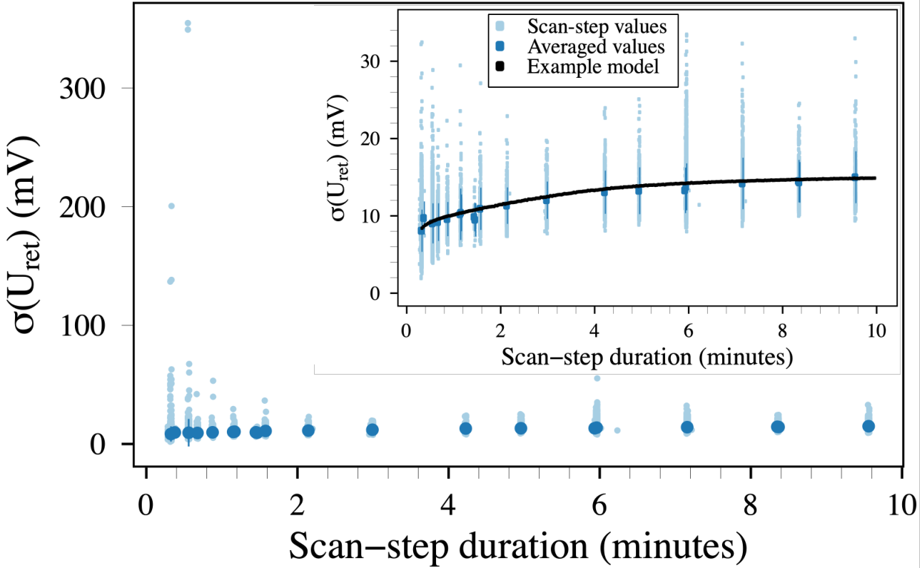
The retarding potential is continuously monitored during the measurements. Therefore, at each scan step, the time evolution of the retarding potential is known with ppm precision. Neglecting this in the analysis introduces an additional broadening of the energy scale, leading to a neutrino-mass shift of $\Delta m_{\nu}^{2}=$ $-3\text{\times}{10}^{-3}\text{\,}{\mathrm{eV}}^{2}$. This shift is less than half the allotment for the high-voltage-related systematic uncertainty in the KATRIN uncertainty budget for full five-year statistics Angrik et al. 2005, and can be neglected in the KNM1 analysis.

The FPD records a low-resolution, differential spectrum of electrons that have passed the high-resolution energy threshold set by the main spectrometer. Measuring the integrated tritium $\upbeta$ spectrum for KNM1, and thereby extracting the neutrino mass, requires an accurate count of electrons that arrive at the FPD within an energy region of interest (ROI) during each scan step. The ROI cut allows rejection of backgrounds and noise events generated near or in the FPD.

When electrons strike the FPD, its pixels are triggered individually, with thresholds set just above the noise floor at around $5\text{\,}\mathrm{keV}$. As described in detail in earlier work Amsbaugh et al. 2015, the energy and timing for each pulse are reconstructed online using a double trapezoidal filter and then recorded; FPD waveforms are not saved during normal operations. The shaping length of the trapezoidal-filter pair is set to $1.6$ $\mu$s, optimizing the energy resolution at around $1.8\text{\,}\mathrm{keV}$ (full width at half maximum, FWHM). During $\upbeta$ scans, rates are too low for significant pileup, but severe pileup during high-rate e-gun measurements can result in deadtime when multiple coincident events drive the baseline out of the ADC dynamic range. This effect is mitigated by individually adjusting the gain of each channel to approximately $5$ ADC counts per $\mathrm{keV}$, preserving good energy resolution while defining a dynamic range (up to $400\text{\,}\mathrm{keV}$) sufficient to accommodate pileup. These settings were implemented in the DAQ firmware prior to the KNM1 measurement. Simulations of the readout chain show that the fraction of time during which the baseline is shifted out of the ADC input range is less than $0.05\text{\,}\mathrm{\%}$ for $50\text{\,}\mathrm{k}\mathrm{c}\mathrm{p}\mathrm{s}$ of $28.6\text{\,}\mathrm{keV}$ electrons, a 100-fold improvement compared to previous settings.

Out of the $148$ pixels, we define a list of $117$ selected detector pixels, distributed as shown in Fig. 5. The excluded pixels are either noisy, or shadowed by beamline instrumentation in the $\upbeta$-electron path along the magnetic flux tube.

Electrons that transit the spectrometer (Sec. V) receive an additional $10\text{\,}\mathrm{keV}$ of kinetic energy from the post-acceleration electrode, and $120\text{\,}\mathrm{eV}$ from the bias voltage applied to the FPD. For a retarding potential around $18.6\text{\,}\mathrm{kV}$, this results in a broad peak in the FPD energy spectrum at around $28\text{\,}\mathrm{keV}$ (Fig. 6). Background electrons and $\upbeta$ electrons share this characteristic energy spectrum in the FPD, since the primary background during KNM1 arises from low-energy electrons that are created inside the main spectrometer and then accelerated by the retarding potential (Sec. VI). The FPD energy scale is calibrated with a ²⁴¹Am gamma source every two weeks.

Our ROI is defined as [$14\text{\,}\mathrm{keV}$, $32\text{\,}\mathrm{keV}$], as measured by the FPD (Fig. 6). The upper bound of the ROI is determined simply from the peak position and the peak width; the lower bound is determined for stability and robustness. In contrast to earlier studies that considered backgrounds originating near the detector Amsbaugh et al. 2015, the choice of a low-energy KNM1 ROI lower bound does not reduce the signal-to-background ratio, since an energy cut cannot differentiate between $\upbeta$ electrons and main-spectrometer background. A cut far away from the peak, where the spectrum shape derivative is small, improves stability against fluctuations of energy scale and resolution. Consequently, corrections for peak-position dependence on retarding potential are negligible.

The specific lower bound of the ROI, $14\text{\,}\mathrm{keV}$, was chosen so as to cancel two effects that arise from charge sharing, in which energy from a single incident electron is divided between two neighboring pixels. If a pixel loses more than half the event charge, its loss from the ROI decreases the effective rate; if a pixel receives more than half the event charge, its inclusion in the ROI increases the effective rate. With the FPD threshold set at half the peak energy, these two effects exactly compensate each other.

Following each pixel trigger (Sec. III.5), the DAQ records the trigger timestamp from a $20\text{\,}\mathrm{MHz}$ clock and the energy information as raw ADC counts integrated over the shaping time of the trapezoidal filter. A scan is divided into scan steps. Each scan step is defined by its HV set point, and its duration is determined according to the measurement-time distribution of the scan (Sec. III.7). Prior to acquisition start at each scan step, handshakes between the DAQ and the HV control system ensure that the HV read-back value has reached the set-point value within a defined accuracy of $50\text{\,}\mathrm{mV}$, as measured by a four-point moving average over the last $8\text{\,}\mathrm{s}$. The inter-spectrometer electron catcher is inserted and removed during this change of scan steps, so that it does not obstruct the beamline during data-taking. A series of pulse-per-second (PPS) pulses from a precision clock synchronized to the Global Positioning System (GPS) defines both the start and stop times of scan steps, providing boundary time accuracy better than $1\text{\,}\mathrm{ns}$. The $50\text{\,}\mathrm{ns}$ digitization timestamps are also phase-locked to $10\text{\,}\mathrm{MHz}$ pulses from the same precision clock. The readout system is capable of handling a pixel rate of $100\text{\,}\mathrm{k}\mathrm{c}\mathrm{p}\mathrm{s}$ and a total rate of $3\text{\,}\mathrm{M}\mathrm{c}\mathrm{p}\mathrm{s}$. Therefore, no deadtime is expected for the actual tritium scan, which has a maximum count rate of $7\text{\,}\mathrm{k}\mathrm{c}\mathrm{p}\mathrm{s}$. A typical two-hour scan produces roughly $120\text{\,}\mathrm{M}\mathrm{B}$ of data.

Immediately after completion of a scan, data files are processed automatically. This processing includes the transfer to storage computers, time-wise event sorting, conversion to offline data formats, and indexing into a run database, followed by automated user-side analysis including the reduction of data in user-specified data files. Except for the handshakes between the DAQ and HV systems, slow-control channels are independent from the tritium scans. Each slow-control sensor has a defined recording interval, typically between $2$ and $10\text{\,}\mathrm{s}$. This is a heterogeneous system for which timestamps are taken from computer timestamps synchronized to the Network Time Protocol (NTP). In the offline analysis, special care is taken for synchronization among different slow-control channels, as well as between the DAQ and slow controls.

An intermediate data layer, consisting of user-side shared data storage with version management, splits the data analysis chain. The first half of the chain covers analysis at the event and time-series levels, and the second half provides higher-level analysis including model fitting. For each scan, results of the first-level analysis are summarized in digest files that contain analyzed FPD counts with efficiency corrections, individual scan steps, calibrated slow-control values (including LARA isotopolog concentration and column density, and analyzed rates extracted from $\upbeta$-induced x-ray spectroscopy and the forward beam monitor), and data-quality flags. Some experimental parameters, such as beamline alignment information and magnetic- and electric-field values determined by measurements and simulations, are shared across all scans in a given measurement period; each such period is summarized in a digest file containing the values of these parameters.

During data-taking, acquisition occasionally began before the HV readback values achieved stability due to minor synchronization errors. The first two seconds of every scan step were removed from the data to address these issues. Count-rate, livetime, efficiency, and stability calculations are performed after these data-quality cuts.

KATRIN measures the integral tritium $\upbeta$ decay spectrum by sequentially applying different retarding energies $qU$, or equivalently HV settings, to the main spectrometer and counting the rate of transmitted $\upbeta$ electrons, $R(qU)$, with the FPD. Our choice of the scan steps – that is, the HV set points and the measurement time at each set point – maximizes the sensitivity for $m^{2}_{\nu}$ by focusing on a narrow region where the impact of the neutrino mass on the spectrum is most pronounced. The location of this region depends on the experimental conditions; in the KNM1 campaign, it lies at $\mbox{$E_{0}$}-$$14\text{\,}\mathrm{eV}$ Kleesiek et al. 2019.

Figure 7 shows the measurement-time distribution used during this campaign, developed using a nominal value of $\mbox{$E_{0}$}{}=$ $18\,574\text{\,}\mathrm{eV}$. The spectrum is scanned repeatedly over the range $[\mbox{$E_{0}$}-$$91\text{\,}\mathrm{eV}$, $\mbox{$E_{0}$}+$$49\text{\,}\mathrm{eV}$$]$ by sequentially applying the non-equidistant HV values (each constituting one scan step) to the main spectrometer. A complete set of measurements at all $39$ scan steps is defined as a scan. Each scan over this energy range takes approximately $2.5\text{\,}\mathrm{h}$ and is performed in alternating upward and downward directions. This mitigates the effects of any time-dependent drifts of the slow-control parameters. As explained in Sec. VIII.9, the analysis interval is limited to an energy range of $[\mbox{$E_{0}$}-$$37\text{\,}\mathrm{eV}$, $\mbox{$E_{0}$}+$$49\text{\,}\mathrm{eV}$$]$, consisting of $27$ scan steps. A brief, additional scan step at $\mbox{$E_{0}$}-$$201\text{\,}\mathrm{eV}$ is used for rate-stability monitoring.

For each tritium scan, we apply quality cuts to relevant slow-control parameters to select a data set with stable run conditions. As Sec. VII describes in detail, data from all active detector pixels are summed, effectively converting the detector wafer into a single, uniform pixel for analysis. Furthermore, all 274 scans are combined by summing counts from like scan steps, forming a single spectrum for fitting.

The $27$ scan steps within the analysis interval cover a total measurement time of $521.7\text{\,}\mathrm{h}$, corresponding to $2.03\text{\times}{10}^{6}\text{\,}\mathrm{e}\mathrm{v}\mathrm{e}\mathrm{n}\mathrm{t}\mathrm{s}$. Table 2 summarizes key operational parameters and figures for events and scans, covering both the full interval and the analysis interval. The evolution of the integrated $\upbeta$-decay luminosity over the course of KNM1 is displayed in Fig. 8.

In KATRIN’s molecular source, the $\upbeta$ decay parent in Eq. 1 becomes ${\mathrm{T}_{2}}{}$, with a molecular decay product ${}^{3}\mathrm{HeT}^{+}$. To model the resulting differential $\upbeta$ spectrum, we begin with a point-like Fermi interaction, which causes the weak decay, and then apply the sudden approximation, in which the Coulomb interaction of the $\upbeta$ electron with the remaining molecular system ${}^{3}\mathrm{HeT}^{+}$ is neglected. The validity of this approximation was demonstrated in Refs. Saenz and Froelich 1997a; Saenz and Froelich 1997b.

Beyond the molecular effects discussed in detail in Sec. IV.2, theoretical corrections to the tritium $\upbeta$ decay spectrum arise at the particle, nuclear, and atomic levels (see Ref. Mertens et al. 2015 for details). Of these, we include only the radiative corrections Repko and Wu 1983 in this work; these have by far the largest effect on the high-energy tail of the $\upbeta$ electron spectrum.

Finally, the electron spectrum $R_{\mathrm{\upbeta}}$ is Doppler-broadened due to the finite motion of tritium molecules in the source. To account for this effect, we replace each discrete final state with a Gaussian centered at the final-state energy $V_{f}$, normalized to $\zeta_{f}$ and with a standard deviation of $94\text{\,}\mathrm{m}\mathrm{e}\mathrm{V}$ according to the Doppler broadening at $30\text{\,}\mathrm{K}$. Effects due to the bulk gas flow are negligible.

For effects that give rise to continuous modifications of the spectrum, such as the molecular final-state distribution and Doppler broadening, a mistake in the modeled variance will introduce a bias on the extracted neutrino-mass squared according to Eq. 7.

Within the sudden approximation, the $\upbeta$ decay effectively corresponds to a sudden change of the nuclear charge of one of the tritium nuclei. This induces electronic and vibrational excitations of the daughter molecular ion ${}^{3}\mathrm{HeT}^{+}$, possibly including its dissociation and/or ionization. Furthermore, the departing $\upbeta$ electron and neutrino induce external (translational) and internal (rotational, vibrational, and – to a smaller extent, neglected here – electronic) excitations.

Since only the energies of the $\upbeta$ electrons are analyzed by KATRIN, the undetected energy associated with the remaining molecular system must be computed ab initio by first solving the Schrödinger equation for the initial and final molecular systems, and then computing the transition probabilities $\zeta_{f}=\absolutevalue{\transitionMatrix_f^\mathrm{mol}}^{2}$ to the molecular daughter states $f$ thus found. Earlier calculations either focused on lower temperatures than KATRIN’s $30\text{\,}\mathrm{K}$ Saenz et al. 2000, thus artificially constraining the population of initial molecular states, or did not include all the tritium-containing isotopologs Doss et al. 2006. In the following, we provide only a minimal description of the new computations carried out for the initial gas states relevant to KATRIN; a detailed publication is in preparation Sibille et al. 2021. The theoretical prediction of the dissociation probability of the daughter ${}^{3}\mathrm{HeT}^{+}$ ion, following $\upbeta$ decay, has recently been experimentally verified Lin et al. 2020.

The transmission condition for any electromagnetic configuration of the KATRIN MAC-E filter determines whether an electron with starting energy $E$ and starting angle $\theta$ is transmitted through a retarding potential $U$:

Only electrons with sufficient surplus energy satisfy the transmission condition and are included in the measured integral spectrum. The KATRIN main spectrometer achieves a magnetic-field ratio $B_{\mathrm{min}}/B_{\mathrm{max}}\approx 1/6700\approx\Delta E/E$, corresponding to a filter width (energy resolution) of $\Delta E=$2.8\text{\,}\mathrm{eV}$$ at $18.6\text{\,}\mathrm{keV}$. The maximum acceptance angle $\theta_{\mathrm{max}}=\arcsin{\sqrt{B_\mathrm{S}/B_\mathrm{max}}}\approx$$$ limits the range of pitch angles contributing to the integral spectrum. The magnetic fields and the retarding potential are provided by detailed field calculations using the Kassiopeia software Furse et al. 2017. To compute the precise electromagnetic fields across the analyzing plane, we use an as-built geometry of the beamline magnets with a detailed three-dimensional model of the main spectrometer. The resulting transmission conditions can be included in the model individually for each active pixel.

The detailed response function of the KATRIN apparatus is calculated from Eq. 13, as modified by energy losses $\epsilon$ between source and analyzing plane Kleesiek et al. 2019:

In an isotropic source like the WGTS, electrons are emitted with an angular distribution $\omega(\theta)d\theta=\sin\theta d\theta$, and we can define an integrated transmission function $T(E,U)$:

Although analysis of non-isotropic e-gun data requires the full expression in Eq. 14, the neutrino-mass analysis in this work exploits the isotropic nature of the tritium $\upbeta$-source and uses the simplified response function

The theoretical total inelastic-scattering cross section of electrons with ${\rm T_{2}}$ molecules in the high-energy Born approximation can be written as Inokuti 1971; Liu 1973; Liu 1987:

where $R_{\mathrm{H}}=$ $13.606\text{\,}\mathrm{eV}$ is the Rydberg energy, $a_{0}^{2}=$ $28.003\text{\times}{10}^{-18}\text{\,}{\mathrm{cm}}^{2}$ the Bohr radius squared, and $E_{\rm nr}$ denotes the non-relativistic kinetic energy of the electron: $E_{\rm nr}=0.5\,\mbox{$m_{\mathrm{e}}$}\beta^{2}$, with $\beta^{2}=1-m^{2}_{\rm e}/(\mbox{$m_{\mathrm{e}}$}+E)^{2}$ and $E$ the relativistic kinetic energy of the electron. At the spectral endpoint for molecular tritium $\upbeta$ decay, we take $E=E_{0}=$ $18.575\text{\,}\mathrm{keV}$ and $E_{\rm nr}=$ $17.608\text{\,}\mathrm{keV}$.

The dominant parameter $M_{\rm tot}^{2}$ can be calculated reliably and with high accuracy, since it is a special electron expectation value for the ground-state hydrogen-molecule wave function. For the three isotopologs, we have Kolos and Wolniewicz 1964; Pachucki: $M_{\rm tot}^{2}[{\rm H_{2}}]=$ $1.5497$, $M_{\rm tot}^{2}[{\rm D_{2}}]=$ $1.5404$ and $M_{\rm tot}^{2}[{\rm T_{2}}]=$ $1.5363$. The calculation of the subdominant parameter $c_{\rm tot}$ is more difficult, and we use the 1987 value of Liu Liu 1987: $c_{\rm tot}=$ $1.18$. With these numbers, we obtain $\sigma_{\rm inel}[{\rm T_{2}}](E_{0})=$ $3.64\text{\times}{10}^{-18}\text{\,}{\mathrm{cm}}^{2}$, with an estimated uncertainty of $0.5\text{\,}\mathrm{\%}$. It must be noted that this theoretical cross section differs from the measured value, $3.40(\pm 0.07)\text{\times}{10}^{-18}\text{\,}{\mathrm{cm}}^{2}$ Aseev et al. 2000, by $7\text{\,}\mathrm{\%}$ ($3.5\text{\,}\sigma$). However, it is $\rho d\sigma$, directly measured by the e-gun as described in Sec. III.2, which is used in the neutrino-mass analysis – not $\sigma$ as a separate input.

Electrons traversing the WGTS can scatter elastically or inelastically from tritium molecules before being analyzed in the main spectrometer. (Here, “elastic” scattering refers to interactions that do not change the electronic state of the molecule.) While elastic scattering only causes a small broadening of the measured response function ($\sim$$0.03\text{\,}\mathrm{eV}$), inelastic scattering can result in energy losses from $\sim$$11\text{\,}\mathrm{eV}$ up to $E/2$, where the lower bound is associated with the lowest electronic excitations in T₂.

Small inelastic energy losses, in particular, can move electrons emitted at energies close to the endpoint (the sensitive region for m${}_{\nu}^{2}$) into a region still within the analysis interval extending $37\text{\,}\mathrm{eV}$ below the endpoint. Precise knowledge of the energy loss spectrum is, therefore, a crucial input for the KATRIN response function. During planning, its uncertainty was estimated to be one of the dominant systematics of the experiment Angrik et al. 2005. A detailed paper on the energy-loss determination is in preparation Aker et al. 2021b.

Various electronic excitations, in combination with rotational and vibrational states of the T₂ molecule, result in a rich spectrum up to the ionization threshold at $15.486\text{\,}\mathrm{eV}$ Weck et al. 1999. Prior to this work, there were no calculations of the energy-loss spectrum with the required accuracy. We therefore measured the energy-loss function with the e-gun installed in the rear system of the KATRIN beamline. In contrast to $\upbeta$ electrons originating within the source, these calibration electrons start with an adjustable kinetic energy chosen close to the endpoint of the tritium $\upbeta$ spectrum and traverse the full length of the source. The dependence of the energy-loss function on the kinetic energy of the electrons can be neglected within the small fit window around the endpoint at $\sim$$18.6\text{\,}\mathrm{keV}$.

The e-gun uses a pulsed ultraviolet laser to create photoelectrons from a gold layer deposited onto the front face of an optical fiber. These electrons are then accelerated in an electric field with an adjustable angle to the local magnetic field lines. The electron energy is continuously scanned, in alternating directions, between $5\text{\,}\mathrm{eV}$ below and $55\text{\,}\mathrm{eV}$ above the main-spectrometer energy threshold $qU$.

The e-gun was operated in two different modes: a fast mode with a $100\text{\,}\mathrm{kHz}$ laser repetition rate to obtain a quasi-continuous electron beam used to record integral spectra as shown in Fig. 11 (top panel)

and a slower mode with a $20\text{\,}\mathrm{kHz}$ repetition rate, in which the electron start times were synchronized with the DAQ to record time-of-flight (TOF) spectra as shown in Fig. 11 (center panel).

This TOF information allows us to record a differential energy spectrum by applying a TOF cut on individual events Bonn et al. 1999. Electrons with energies close to $qU$ take significantly longer to reach the detector since they are decelerated to almost zero kinetic energy near the analyzing plane. Selecting electrons with flight times between $35\text{\,}\mathrm{\SIUnitSymbolMicro s}$ and $50\text{\,}\mathrm{\SIUnitSymbolMicro s}$, as illustrated in Fig. 11 (bottom panel), effectively turns the main spectrometer from a high-pass filter into a narrow band-pass filter with a width of $\sim$$0.02\text{\,}\mathrm{eV}$. Apart from effects of multiple scattering and finite energy resolution, this method provides direct access to the electron energy-loss spectrum.

The energy-loss function is parametrized by a semi-empirical model using three Gaussians to describe the three groups of lines created by excitations of the $(2p\sigma^{1}\Sigma^{+}_{u})$, $(2p\pi^{1}\Pi_{u})$ and $(3p\pi^{1}\Pi_{u})$ molecular states around $12.6\text{\,}\mathrm{eV}$ Geiger 1964 and the binary-encounter-dipole (BED) model Kim and Rudd 1994 to describe the continuous ionization tail at energy losses above $15.5\text{\,}\mathrm{eV}$ (Fig. 11 center). The model has nine parameters given by the mean, width, and strength of each Gaussian. The normalization of the tail is chosen such that one obtains a smooth continuation of the Gaussian part of the model at the ionization energy.

To fit the measured TOF spectra, the model function is first convolved several times with itself, to account for multiple inelastic scatterings in the source, and then with the measured spectrum of unscattered electrons (peak at $0\text{\,}\mathrm{eV}$ in Fig. 11 center). This spectrum of electrons which have not undergone inelastic scattering naturally includes the effects of elastic scattering and the filter width of the main spectrometer. The resulting curves for single and multiple scattering are then weighted with the Poisson-distributed scattering probabilities and summed. The expectation value of this Poisson distribution is a nuisance parameter in the fit. A combined fit of TOF spectra taken at different column densities must also account for differences in the e-gun laser intensity between the individual measurements, leading to changes in the count rate. Additional normalization factors are therefore included as nuisance parameters in the fit. Finally, additional background components are included in the fit. Background electrons produced by the impact of positive ions onto the photocathode of the e-gun, for example, do not exhibit a TOF structure and appear in the differential spectrum as a small additional component with the shape of an integral energy-loss spectrum. The scaling factors of this background are additional nuisance parameters.

We performed a combined fit to four TOF datasets measured at different column densities. Each dataset contains about $12$ hours of data, resulting in $\sim$$6\text{\times}{10}^{5}$ events surviving the TOF cut. The nine model parameters of interest are shared between all datasets, whereas each dataset has its own nuisance parameters as described above.

The resulting best-fit parametrization is shown in Fig. 11 top and center for the integral and differential data, respectively. The same energy-loss function describes all four datasets well and the fit has a reduced $\chi^{2}$ close to one.

Uncertainties used in this work are of a statistical nature only. However, more advanced combined fits that also take into account the integral energy-loss measurements yield the same parameter values within their statistical uncertainties.

Systematic uncertainties in the energy-loss determination are largely canceled by alternating up- and downward scans. A study of systematic effects on the parameter uncertainties has been undertaken using a Monte Carlo (MC) approach and taking into account disturbances like column-density drifts, background events, detector pileup and the binning of the continuous voltage ramp. These systematic uncertainties are negligible for the KNM1 analysis.

An improved parametrization of the energy-loss function and its uncertainties is under investigation for future, more sensitive neutrino-mass campaigns.

The steady-state background originates from excited or unstable neutral atoms which can propagate freely in the ultra-high-vacuum environment of the main spectrometer. It has two primary causes.

First, a significant part of the steady-state background arises from hydrogen Rydberg atoms sputtered from the inner spectrometer surfaces by ²⁰⁶Pb recoil ions following $\upalpha$ decays of ²¹⁰Po. These processes follow the decay chain of the long-lived ²²²Rn progeny ²¹⁰Pb, which was surface-implanted from ambient air (activity $\sim$$1\text{\,}\mathrm{Bq}\text{/}{\mathrm{m}}^{2}$) during the construction phase. A small fraction of these Rydberg atoms is ionized by black-body radiation when propagating through the magnetic flux tube. The resulting sub-$\mathrm{eV}$ scale electrons are accelerated to $qU$ by the MAC-E-filter, adding a Poisson component to $R_{\mathrm{bg}}$.

The second significant steady-state background mechanism originates with $\upalpha$ decays of single ²¹⁹Rn atoms ($t_{1/2}=$ $3.96\text{\,}\mathrm{s}$) emanating from the non-evaporable-getter pumps. Each decay releases a large number of electrons up to the $\mathrm{keV}$ scale. If the decay occurs in the magnetic flux tube, these electrons are stored due to their significant transverse momenta. They subsequently produce secondary electrons by scattering on the residual gas until they have cooled to energies of a few $\mathrm{eV}$, when they can escape; both primary and secondary electrons contribute to $R_{\mathrm{bg}}$ at $qU$ Frankle et al. 2011. Since several background electrons may originate from each ²¹⁹Rn decay in the magnetic flux tube, this background source is not purely Poissonian. Liquid-nitrogen-cooled copper baffles at the ports to the getter pumps mitigate this effect by preventing ²¹⁹Rn from diffusing into the sensitive volume Harms 2015; Görhardt et al. 2018. Due to the formation of a thin layer of H₂O covering the baffle surface, the retention of ²¹⁹Rn was hampered such that $R_{\mathrm{bg}}$ retains an observable non-Poissonian component during KNM1.

In KNM1, the overall steady-state background rate, $R_{\mathrm{bg}}$, is continuously measured through the energy-independent part of the spectrum R($\langle qU\rangle$). The whole spectrum is fitted, leading to a value over the $117$ selected pixels of $R_{\mathrm{bg}}=$0.293(\pm 0.001)\text{\,}\mathrm{c}\mathrm{p}\mathrm{s}$$ that is largely constrained by the $5$ scan steps above the expected $E_{0}$. This value is consistent with data from independent background runs. Full fit results are given in Sec. IX.4.

The background is not distributed uniformly across the detector, as shown in Fig. 12. The decrease of $R_{\mathrm{bg}}$ towards smaller radii can be explained by radiative de-excitation of the Rydberg atoms as they propagate inside the main spectrometer. Further from the spectrometer wall, fewer Rydberg atoms are therefore available for ionization by the thermal radiation.

The steady-state background was monitored for each $\upbeta$-scan with the five dedicated background-region scan steps. Figure 13 shows the time evolution of these background measurements during KNM1. A linear fit was applied to the data in order to test the long-term stability of the background. The slope of $-0.01(\pm 0.08)\text{\,}\mathrm{m}$ is compatible with a background that is stable over long time scales.

The non-Poissonian component of $R_{\mathrm{bg}}$ causes a broadening of the event distribution of the five background-region scan steps, amounting to $6.4\text{\,}\mathrm{\%}$ compared to the prediction from pure Poisson statistics (Fig. 14).

Our model predicts a background that is independent of $qU$ near $E_{0}$. To test this expectation, we performed a dedicated background-only measurement, without an active tritium source, in June 2018. As shown in Fig. 15, $qU$ was scanned in $26$ steps over an interval of $16.975\text{\,}\mathrm{keV}18.615\text{\,}\mathrm{keV}$. We then fit a line with a free slope parameter to these data. The resulting best-fit slope, $-2.2(\pm 4.3)\text{\,}\mathrm{m}$, is compatible with zero, and we take its uncertainty as an overall uncertainty on our assumption of a $qU$-independent background (Sec. VIII.7).

With both the pre-spectrometer and main spectrometer held at negative retarding potentials, a Penning trap inevitably forms in the strong magnetic field of the grounded inter-spectrometer region. Electrons trapped in this region slowly lose energy by ionizing residual gas molecules. The resulting ions may escape into the main spectrometer, where they can create background electrons when their own collisions with the residual gas or the vessel wall release ionization electrons, Rydberg atoms, or photons. The intense WGTS feeds the Penning trap when $\upbeta$ electrons produce positive ions on their way into the pre-spectrometer; these ions sputter Rydberg atoms from the pre-spectrometer walls, and the Rydberg atoms in turn produce low-energy ionization electrons that fill the trap Aker et al. 2020b. This mechanism may also play a role in main-spectrometer backgrounds, when $\upbeta$ electrons scatter further downstream and the resulting ions strike the main-spectrometer walls.

During each transition to a new scan step, an electron catcher is briefly inserted into the beamline to remove stored electrons from the Penning trap. At higher pre-spectrometer potential, this has been shown to provide a statistically significant reduction in the baseline background Aker et al. 2020b. However, since the electron catcher is inserted only at the beginning of a scan step, the Penning trap continues to fill until a new electron-catcher actuation at the beginning of the next scan step. The corresponding rise of the background rate is strongly influenced by surface conditions and by the achieved pressure between the spectrometers. In principle, however, this mechanism can produce a background that effectively increases in rate for longer-duration scan steps (see measurement-time distribution in Fig. 7). This effect was observed in a subsequent KATRIN scientific run, but for KNM1 – the initial science run, with pristine surfaces and lower column density – no statistically significant dependence on scan-step duration was observed. Section VIII.7 will address the impact on the neutrino-mass measurement.

During KNM1, the electric potential and magnetic field in the analyzing plane of the main spectrometer were not perfectly homogeneous, but varied radially by about $140\text{\,}\mathrm{mV}$ and $2\text{\,}\mathrm{\SIUnitSymbolMicro T}$, respectively, and to a much smaller extent azimuthally. The pixelation of the detector allows us to account for these spatial dependencies. Each pixel has a specific transmission function and records a statistically independent tritium $\upbeta$-electron spectrum. In this analysis, we combine these pixel-wise spectra into a single effective pixel by adding all counts and assuming an average transmission function for the entire detector. The averaging of fields leads to a negligible broadening of the spectrum which does not affect the filter width, and carries a negligible bias of $\mathcal{O}(${10}^{-3}\text{\,}\mathrm{eV}$)$ on $m^{2}_{\nu}$.

Combining all 274 scans that passed data-quality cuts, single-pixel fits were performed resulting in an endpoint $E^{\text{fit}}_{0}$ for each pixel, as shown in Fig. 16. We find no systematic spatial (i.e. pixel) dependence of $E^{\text{fit}}_{0}$. The standard deviation from the mean endpoint is $0.16\text{\,}\mathrm{eV}$, which is consistent with statistical fluctuations. This indicates a good description of the electric potential and magnetic field in the analyzing plane, and the absence of a significantly spatially dependent electron starting potential. We therefore merge the data of all $117$ selected pixels used in the analysis (Fig. 5).

Combining all pixels in a uniform fit, we can now consider the stability of the fit parameters with respect to possible temporal variations. We investigate all four free parameters in the fit. For single scans of $2$ hours, the accumulated statistics are not sufficient to significantly constrain the neutrino mass. Therefore, the neutrino mass is fixed to zero. The $274$ fit values show excellent stability over the course of a month (Fig. 17). The standard deviation from the mean endpoint is $0.25\text{\,}\mathrm{eV}$, which is again consistent with statistical fluctuations.

In order to constrain the neutrino mass, the statistics of all $274$ scans must be combined. Based on our stability results, we achieve this by merging the data of all $274$ scans into a single stacked, integral spectrum. In the underlying process, the events at like scan steps are summed and the corresponding retarding-potential values are averaged over all scans. This procedure yields one high-statistics integral spectrum with the same number of scan steps as a single scan. Since this method does not correct for scan-to-scan variations of slow-control parameters, it relies on good time stability and excellent reproducibility of the individual HV settings from scan to scan. The Gaussian spread of these HV settings is on average $\sigma=$ $34(\pm 1)\text{\,}\mathrm{mV}$ (better than 2 ppm) (Sec. III.4). The scan stacking results in a minor systematic effect, which is included in the analysis.

The resulting stacked integral spectrum, R($\langle qU\rangle$), is displayed in Fig. 18. It comprises a total of $2.03\text{\times}{10}^{6}$ events, with $1.48\text{\times}{10}^{6}$ $\upbeta$ decay electrons below $E_{0}$ and a flat background ensemble of $0.55\text{\times}{10}^{6}$ events in the $86\text{\,}\mathrm{eV}$ analysis interval, $[\mbox{$E_{0}$}-$$37\text{\,}\mathrm{eV}$, $\mbox{$E_{0}$}+$$49\text{\,}\mathrm{eV}$$]$.