Nir Shlezinger, Nariman Farsad, Yonina C. Eldar, and Andrea J. Goldsmith
Chapter 1 Model-Based Machine Learning for Communications
Nir Shlezinger
Nariman Farsad
Yonina C. Eldar
Andrea J. Goldsmith
1 Introduction
Traditional communication systems design is dominated by methods that are based on statistical models. These statistical-model-based algorithms, which we refer to henceforth as model-based methods, rely on mathematical models that describe the transmission process, signal propagation, receiver noise, interference, and many other components of the system that affect the end-to-end signal transmission and reception. Such mathematical models use parameters that vary over time as the channel conditions, the environment, network traffic, or network topology change. Therefore, for optimal operation, many of the algorithms used in communication systems rely on the underlying mathematical models as well as the estimation of the model parameters. However, there are cases where this approach fails, in particular when the mathematical models for one or more of the system components are highly complex, hard to estimate, poorly understood, do not well-capture the underlying physics of the system, or do not lend themselves to computationally-efficient algorithms. In some other cases, although mathematical models are known, accurate parameter estimation may not be possible. Finally, common hardware limitations, such as the restriction to utilize low-resolution quantizers or non-linear power amplifiers, can significantly increase the complexity of the underlying channel model.
An alternative data-driven approach is based on ml (ml). ml techniques, and in particular, deep learning, have been the focus of extensive research in recent years due to their empirical success in various applications, including computer vision and speech processing [1, 2]. The benefits of ml-driven methods over traditional model-based approaches are threefold: First, ml methods are independent of the underlying stochastic model, and thus can operate efficiently in scenarios where this model is unknown or its parameters cannot be accurately estimated. Second, when the underlying model is extremely complex, ml algorithms have demonstrated the ability to extract and disentangle the meaningful semantic information from the observed data [3], a task which is very difficult to carry out using traditional model-based approaches, even when the model is perfectly known. Finally, the main complexity in utilizing ml methods is in the training stage, which is typically carried out offline. Once trained, they tend to implement inference at a lower computational burden and delay compared to their analytical model-based counterparts [4].
Although ml has been the focus of significant research attention over the last decade, it has yet to significantly contribute to practical designs in one of the most important technologies of the modern era – digital communication. The fact that ml-based algorithms, which have revolutionized the fields of computer vision and natural language processing, do not yet play a fundamental role in the design of physical layer communication systems, and particularly digital receivers, may be due to one or more of the following reasons:
- 1.
The large amount of possible outputs impose a major challenge in efficiently applying ml algorithms. In particular, the constellation size of the modulation and the blocklength of the channel code, combined with the time-varying nature of communication channels, leads to an exponentially large number of possible channel outputs that an ml receiver algorithm must be trained on.
- 2.
Traditional deep learning techniques require high computational resources, while communication devices, such as wearable devices and mobile phones, are typically limited in hardware and power.
- 3.
To date, conventional communication schemes, which assume a simplified channel model with parameters that are dynamically estimated, have been very successful.
The third reason is likely to become less relevant as the spectrum congestion of existing cellular standards forces future communication systems to explore new frequency ranges and share spectrum with other application such as radar [5]. As these new frequency bands and spectrum sharing techniques become widespread, the simplified channel, interference, and noise models used in current communication receiver techniques may no longer work well. Moreover, the strict cost, power, and memory constraints imposed on communicating devices lead to the usage of low-resolution adc and power amplifiers with dominant non-linearities [6]. This makes the successful application of model-based techniques significantly more complex. Thus, conventional model-based approaches may no longer be able to meet the performance and throughput demands of future wireless devices, motivating their combination with data-driven approaches based on ml such as deep learning. Such techniques must still overcome the challenges identified above with respect to the large computational resources and data sets needed for training.
Despite its unprecedented success, deep learning is subject to several challenges which limit its applicability in some important communication scenarios. In particular, dnn consist of highly-parameterized systems that can represent a broad range of mappings. As such, massive data sets are typically required to learn a desirable mapping, and the computational burden of training and utilizing these networks may constitute a major drawback. For example, consider the two receivers illustrated in Fig. 1, which carry out symbol detection using model-based algorithms and model-agnostic dnn, respectively. The dynamic nature of wireless channels implies that the receivers should track channel variations in order to reliably detect the transmitted messages over long periods of time. To do so, the model-based receiver in Fig. 1(a) typically estimates the model parameters imposed on the underlying statistics using periodic pilots. For the same purpose, the dnn-based receiver in Fig. 1(b) should periodically re-train its dnn to track channel variations. The fact that doing so requires a large data set leads to a significant decrease of spectral efficiency and increase in computational complexity associated with this training. Furthermore, dnn are commonly utilized as black-boxes, and thus do not offer the interpretability, flexibility, versatility, and reliability of model-based techniques.

The limitations associated with model-based methods and black-box deep learning systems gave rise to a set of techniques on the interface of traditional model-based communication and ml, attempting to benefit from the best of both worlds [7]. Such model-based ml systems can be divided into two main categories. The first of the two utilizes model-based methods as a form of domain knowledge in designing a dnn architecture, which is then trained and used for inference. The most common example of this strategy is the family of deep unfolded networks [8, 9], which design the layers of a dnn to imitate the iterations of a model-based optimization algorithm, and has been utilized in various communication-related tasks [10]. The second strategy, which we call dnn-aided hybrid algorithms, uses model-based methods with integrated dnn for inference by incorporating ml in a manner that makes the system more robust and model-agnostic. Communication receivers designed using dnn-aided inference include the data-driven implementations of the Viterbi algorithm [11] and the BCJR detector [12].
In this chapter we present an introduction to model-based ml for communication systems. We begin by reviewing existing strategies for combining model-based algorithms and ml from a high level perspective in Section 2, and compare them to the conventional deep learning approach which utilizes established dnn architectures trained in an end-to-end manner. Then, in Section 3 we focus on symbol detection, which is one of the fundamental tasks of communication receivers. We show how each strategy, i.e., conventional dnn architectures, deep unfolding, and dnn-aided hybrid algorithms, can be applied to this problem. The last two approaches constitute a middle ground between the purely model-based and the dnn-based receivers illustrated in Fig. 1. By focusing on this specific task, we highlight the advantages and drawbacks of each strategy, and present guidelines to facilitate the design of future model-based deep learning systems for communications. We conclude this chapter with a summary provided in Section 4.
2 Model-Based Machine Learning
We begin by reviewing the leading approaches for combining ml, and particularly deep learning, with model-based algorithms. The neural networks in this hybrid-approach are trained in a supervised manner and then used during inference. Then, in Section 3 we focus on symbol detection and provide concrete examples on how this approach can be used to design data-driven detectors.
In a broad family of problems, a system is required to map an input variable into a prediction of a label variable . ml systems learn such a mapping from a training set consisting of pairs of inputs and their corresponding labels, denoted . Model-based methods carry out such inference based on prior knowledge of the statistical model relating and , denoted . Model-based ml systems reviewed in this chapter combine model-based methods with learning techniques, namely, they tune their mapping of the input based on both a labeled training set as well as some knowledge of the underlying distribution. Such hybrid data-driven model-aware systems can typically learn their mappings from smaller training sets compared to purely model-agnostic dnn, and commonly operate without full and accurate knowledge of , upon which model-based methods are based. We next elaborate on the main strategies of combining ml and model-based techniques, beginning with extreme cases of dnn that rely solely on data and purely model-based inference algorithms.
2.1 Conventional Deep Learning
The conventional application of deep learning is to carry out inference using some standard dnn architecture. This dnn uses the training data to learn how to map a realization of the input into a prediction . Such highly-parameterized networks can effectively approximate any Borel measurable mapping, as it follows from the universal approximation theorem [13, Ch. 6.4.1]. Therefore, by properly tuning their parameters using a sufficiently large training set, typically using optimization based on some variant of sgd (sgd), one should be able to obtain the desirable inference rule.
While standard dnn structures are highly model-agnostic and are commonly treated as black-boxes, one can still incorporate some level of domain knowledge in the selection of the specific network architecture. For instance, when the input is known to exhibit temporal correlation, architectures based on rnn or transformers are known to be preferable. Alternatively, in the presence of spatial patterns, one may prefer to utilize convolutional layers. An additional method to incorporate domain knowledge into a black-box dnn is by pre-processing of the input via, e.g., feature extraction.
Conventional deep learning based on established black-box dnn is data-driven, i.e, it requires data representing the problem at hand, possibly combined with a very basic level of domain knowledge to select the specific architecture. A major drawback of using such networks, which is particularly relevant in the context of communication systems, is that learning a large number of parameters requires a massive data set to train. In dynamic environments, even when a sufficiently large data set is available, it is difficult to train a model that performs optimally over the whole range of the dynamically changing system. Moreover, online training as the system dynamics change tends to be computationally expensive because of the large number of parameters.
2.2 Model-Based Methods
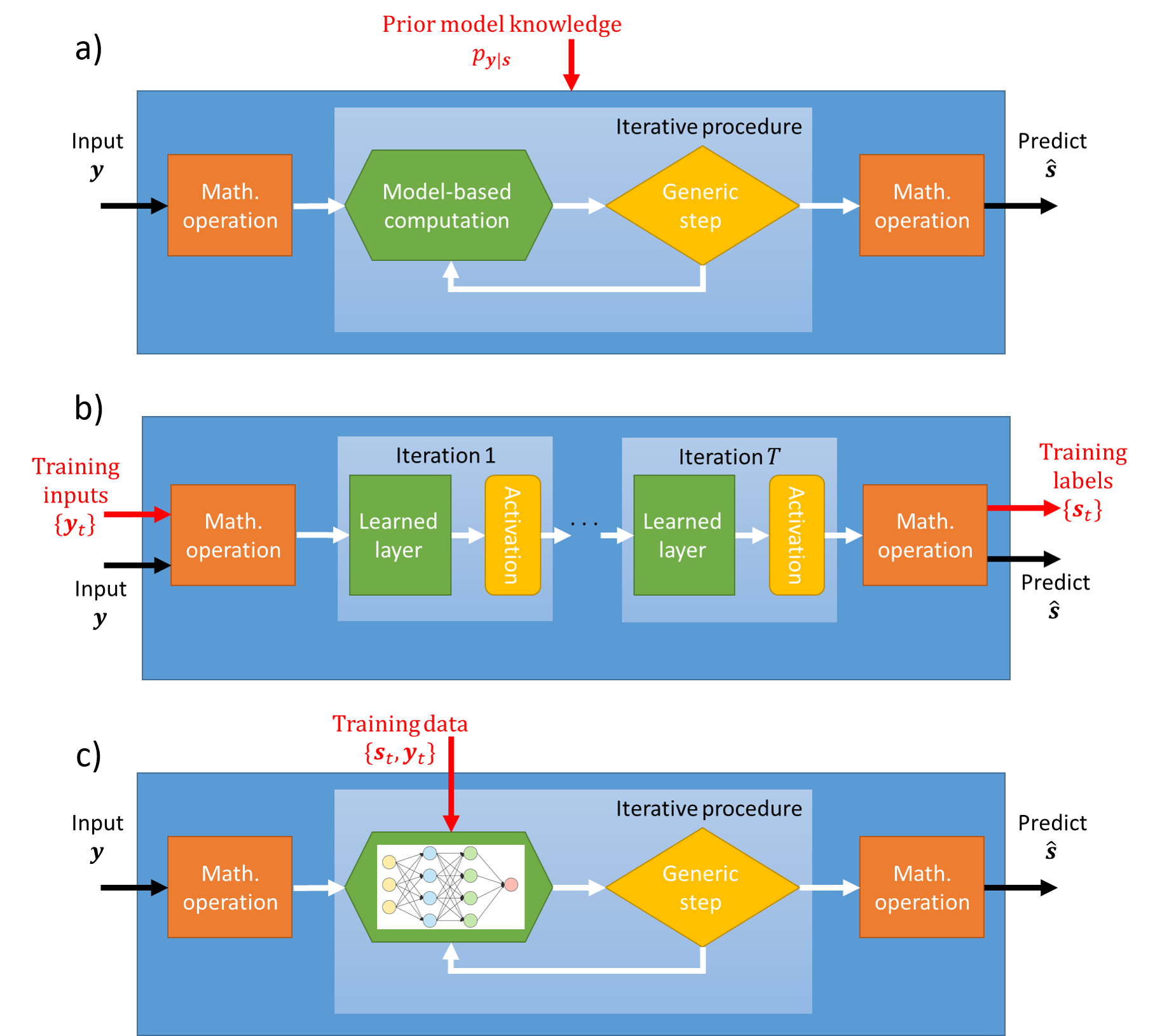
Model-based algorithms carry out inference based on prior knowledge of the underlying statistics relating the input and the label , i.e., . A common family of model-based methods is based on iterative algorithms, which allow us to infer with provable performance and controllable complexity in an iterative fashion, as illustrated in Fig. 2(a). This generic family of iterative algorithms consists of some input and output processing stages, with an intermediate iterative procedure. The latter can in turn be divided into a model-based computation, namely, a procedure that is determined by ; and a set of generic mathematical manipulations.
These algorithms vary significantly between different statistical models. For instance, for the symbol detection task, model-based methods such as the Viterbi detector [14] or the BCJR algorithm [15] are valid for finite-memory channels, while for mimo (mimo) detection one may utilize the family of interference cancellation methods [16]. Each such algorithm may be specifically tailored to a given scenario, as opposed to black-box dnn, in which the parameterized inference rule is generic, and the unique characteristics of the scenario at hand are encapsulated in the parameters learned during training.
Model-based techniques do not rely on data to learn their mapping, though data is often used to estimate unknown model parameters. In practice, accurate knowledge of the statistical model relating the observations and the desired information is typically unavailable, and thus applying such techniques commonly requires imposing some assumptions on the underlying statistics, which in some cases reflects the actual behavior, but often do not. In the presence of inaccurate knowledge of due to estimation errors or due to enforcing a model that does not fully capture the environment, the performance of model-based methods tends to degrade considerably. This limits the applicability of model-based algorithms in scenarios where is unknown, costly to estimate accurately, or too complex to express analytically.
2.3 Model-Based Deep Learning by Deep Unfolding
Deep unfolding [8, 9], also referred to as deep unrolling, is a common strategy to combine deep learning with model-based algorithms. Here, model-based methods are utilized as a form of domain knowledge in designing a dnn architecture, which is trained end-to-end and then used for inference. Unlike the application of conventional black-box dnn discussed in Section 2.1, deep unfolding utilizes a unique dnn structure designed specifically for the task at hand.
The main rationale in deep unfolding is to design the network to imitate the operation of a model-based iterative optimization algorithm corresponding to the considered problem. In particular, each iteration of the model-based algorithm is replaced with a dedicated layer with trainable parameters whose structure is based on the operations carried out during that iteration. An illustration of a neural network obtained by unfolding the model-based iterative model of Fig. 2(a) is depicted in Fig. 2(b), where a network with layers is designed to imitate iterations of the optimization method. Once the architecture is fixed, the resulting network is trained in an end-to-end manner as in conventional deep learning.
Deep unfolded networks, in which the iterations consist of trainable parameters, are typically capable of inferring with a smaller number of layers compared to the amount of iterations required by the model-based algorithm. Consequently, even when the model-based algorithm is feasible, processing through a trained unfolded dnn is typically faster than applying the iterative algorithm [4]. Furthermore, converting a model-based algorithm into an unfolded deep network can also improve its performance. For example, iterative algorithms based on some relaxed optimization commonly achieve improved accuracy when unfolded into a dnn, due to the ability to learn to overcome the error induced by relaxation in the training stage. The main benefits of deep unfolding over using end-to-end networks stem from its incorporation of domain knowledge in the network architecture. As such, unfolded networks can achieve improved performance at reduced complexity, i.e., when operating with less parameters, compared to conventional end-to-end networks [10]. Nonetheless, deep unfolded networks are highly parameterized dnn, which often require large data sets for training, though usually not as much as the generic dnn. Furthermore, deep unfolding typically requires a high level of domain knowledge, such as explicit knowledge of the statistical model up to possibly some missing parameters, in order to formulate the optimization algorithm in a manner that can be unfolded.
2.4 Model-Based Deep Learning by dnn-Aided Algorithms
The second strategy for combining model-based methods and deep learning, which we refer to as dnn-aided hybrid algorithms, aims at integrating ml into model-based techniques. Such dnn-aided systems mainly utilize conventional model-based methods for inference, while incorporating dnn to make the resultant system more robust and model-agnostic. This approach builds upon the insight that model-based algorithms typically consist of a set of generic manipulations that are determined by the structure of the statistics, e.g., whether it obeys a Markovian structure. Beside these generic manipulations, there are also computations that require actual knowledge of , as illustrated in Fig. 2(a). Consequently, when one has prior knowledge on the structure of the underlying distribution but not of its actual distribution, ml can be utilized to fill in the missing components required to carry out the algorithm.
In particular, dnn-aided hybrid algorithms start with a model-based algorithm that is suitable for inference when the statistics of are available. For instance, symbol detection over finite-memory channels can be carried out accurately and with affordable complexity using either the Viterbi algorithm [14] or the BCJR method [15], assuming is known. Then, ml-based techniques, such as dedicated dnn, are used to estimate only from data. These dedicated dnn can be trained individually, separately from the inference task, or in an end-to-end manner along with the overall algorithm that maps into an estimate of . An illustration of a dnn-aided algorithm obtained by integrating ml into the iterative methods illustrated in Fig. 2(a) is depicted in Fig. 2(c).
dnn-aided hybrid algorithms have several advantages: First, they use dnn for specific intermediate tasks, such as computing a conditional probability measure, which are much simpler compared to end-to-end inference. Consequently, relatively simple networks that are trainable using small training sets can be used. Furthermore, once trained the system effectively implements the model-based algorithm in a data-driven manner without imposing a model on the underlying distribution and estimating its parameters. Concrete examples of dnn-aided symbol detection algorithms are detailed in Section 3.4.
3 Deep Symbol Detection
In digital communication systems, the receiver is required to reliably recover the transmitted symbols from the observed channel output. This task is commonly referred to as symbol detection. In this section, we present how the strategies for combining ml and model-based algorithms detailed in the previous section can be applied for data-driven symbol detection. We first formulate the symbol detection in Section 3.1, after which we discuss the applications of data-driven receivers based on conventional dnn architectures, deep unfolding, and dnn-aided algorithms, in Sections 3.2-3.4, respectively. For each strategy we begin with the main rationale behind this approach, present at least one concrete example, and discuss its pros and cons. Finally, we numerically compare the data-driven receivers to their model-based counterparts in Section 3.5.
3.1 The Symbol Detection Problem
To formulate the symbol detection problem, we let be the symbol transmitted at time index . Here, represents the blocklength and denotes the number of symbols transmitted at each time instance, e.g., the number of users transmitting simultaneously in the uplink communications channel. Each symbol is uniformly distributed over a set of constellation points, thus . We use to denote the channel output at time index , where represents the number of receive antennas. When both and are larger than one, the resulting setup corresponds to mimo communications. Symbol detection refers to the recovery of from the observed . An illustration of the symbol detection problem using a dnn-aided receiver is depicted in Fig. 3.

We focus on finite-memory stationary causal channels, where each is given by a stochastic mapping of , and is the memory of the channel, assumed to be smaller than the blocklength . The special case in which is referred to as flat or memoryless channel conditions. The conditional pdf (pdf) of the channel output given its input thus satisfies
| (1) |
where the lower-case and represent the realizations of the random variables and , respectively. The fact that the channel is stationary implies that the conditional pdf does not depend on the index .
The symbol detection mapping that minimizes the error rate is the map (map) rule, given by
| (2) |
For the memoryless case , solving (2) reduces to maximizing over . However, when is large, as is commonly the case in uplink mimo systems, solving (2) may be computationally infeasible, even when the pdf is perfectly known. The application of deep learning for symbol detection thus has two main motivations: the first is to allow symbol detection to operate in a model-agnostic manner, i.e., without requiring knowledge of , and the second is to facilitate inference when the computational complexity of (2) renders solving it infeasible.
3.2 Symbol Detection via Established Deep Networks
The first approach to designing data-driven symbol detectors treats the channel as a black-box and relies on well-known deep learning architectures used in computer vision, speech, and language processing for detection. We now describe how conventional deep neural architectures can be used for symbol detection.
3.2.1 Overview of Design Process
Different dnn architectures have shown promising results for detection and estimation in applications such as image processing [17, 18, 19], speech recognition [20, 21, 22], machine translation [23, 24, 25], and bioinformatics [26, 27]. Some of these neural network architectures can be used to design a symbol detector for channels with unknown models using supervised learning. This process typically consists of the following steps:
- 1.
Identify the conventional neural network architectures that are suitable for the channel under consideration, and use these networks as building blocks for designing the detection algorithm. For example, rnn are more suitable for sequential detection in channels with memory, while convolutional and fully-connected networks are more suitable for memoryless channels.
- 2.
Next, use channel input-output pairs to train the network. Two approaches can be used for training: In the first approach, a model is trained for each channel condition (e.g., each SNR). In the second approach, a large training dataset consisting of various channel conditions is used to train a single neural network detector for detection over a wide-range of channel conditions. The training data can be generated by randomizing the transmitted symbols and generating the corresponding received signal using mathematical models, simulations, experiments, or field measurements.
- 3.
Train the overall resulting network in an end-to-end fashion.
We next demonstrate how this rationale is translated into a concrete data-driven symbol detector architecture for finite-memory channels.
3.2.2 Example: SBRNN for Finite-Memory Channels
The sbrnn (sbrnn) is a sequence detection algorithm for finite-memory channels proposed in [28]. Generally, sequence detection can be performed using rnn [1], which are well established for sequence estimation in different problems such as neural machine translation [23], speech recognition [2], or bioinformatics [26]. For simplicity, we assume in our description that the input cardinality is . The estimated symbol in this case is given by
| (3) |
where is the probability of estimating each symbol based on the dnn model used. One of the main benefits of this detector is that after training, it can perform detection on any data stream as it arrives at the receiver. This is because the observations from previous symbols are summarized as the state of the RNN, which is represented by a vector. Note that the observed signal during the th transmission, where , may carry information about the th symbol due to the memory of the channel. However, since RNNs are feed-forward only, during the estimation of , the observation signal is not considered.
One way to overcome this limitation is by using bidirectional RNNs (BRNNs). In such networks, a sequence of received signals are fed once in the forward direction into one RNN cell, and fed once in the backward direction into another RNN cell [29], for some fixed representing the BRNN length. The two outputs are then concatenated and may be passed to more bidirectional layers. A signal whose blocklength is larger than the BRNN length is divided into multiple distinct subsequences of length . Ideally, the must be at least the same size as the memory length . However, if this is not known in advance, the BRNN length can be treated as a hyperparameter to be tuned during training. At time instance belonging to the th subsequence, the estimated symbol for BRNN is given by
| (4) |
To simplify the notation, we use to denote the matrix whose entries are the pmf (pmf) for each .
The BRNN architecture ensures that in the estimation of a symbol, future signal observations are taken into account. During training, blocks of consecutive transmissions are used for training. Once the network is trained, BRNNs detect the stream of incoming data in fixed blocks of length , as shown in the top portion of Fig. 4. The main drawback here is that the symbols at the end of each block may affect the symbols in the next block, and since each block is treated independently, this relation is not captured in this scheme. Another issue is that the block of symbols must be received before detection can be performed. The top portion of Figure 4 shows this scheme for .
To overcome these limitations, in the sbrnn proposed in [28], the first symbols are detected using the BRNN. Then, as each new symbol arrives at the receiver, the subsequence processed by the BRNN slides ahead by one symbol. Let the set be the set of all valid starting positions for a BRNN detector of length , such that the detector overlaps with the th symbol. For example, if and , then is not in the set since the BRNN detector overlaps with symbol positions 1, 2, and 3, and not the symbol position 4. The estimated pmf corresponding to the th symbol is given by the weighted sum of the estimated PMFs for each of the relevant windows:
| (5) |
The weighted sum coefficients can be set to , as we do in the numerical evaluations in Section 3.5. An illustration of the operation of the SBRNN detector based on (5) is depicted in the bottom portion of Fig. 4.
3.2.3 Summary
Well-known dnn architectures can be trained in an end-to-end manner to perform symbol detection. This approach builds upon the success of existing model-agnostic dnn structures, resulting in symbol detectors operating without any knowledge about the underlying channel models. Furthermore, this strategy allows combining some basic level of domain knowledge in the selection of the architecture as well as the preparation of its input. For example, the SBRNN detector detailed above identifies the BRNN architecture as one that is capable of handling temporal correlation in finite-memory channels, while using a sliding subsequence to overcome some of the limitations of BRNN architectures when applied to different blocks independently. Also, dnns can well-capture the nonlinearities that may exist in the channel. For example, the sbrnn was used as an autoencoder in [30, 31] to achieve state-of-the-art performance over optical channels, outperforming model-based nonlinear equalizers such as Voltera. Finally, these networks can also be computationally more efficient than the optimal maximum-likelihood sequence detector over finite-memory channels, specifically for channels with long memory.
The main drawback in using established deep networks for end-to-end symbol detection is that such architectures typically have a very large number of parameters, and thus require massive data sets for training. This renders online training using pilot sequences impractical. Moreover, when they are trained using data from a large set of channel conditions, the resulting network will not perform optimally for each of those channel conditions individually. Furthermore, even when the data set is extremely large and diverse, it is not likely to capture all expected channel conditions. Finally, conventional dnn architectures are treated as black-boxes, and are in general not interpretable, making it difficult to come up with performance guarantees.
3.3 Symbol Detection via Deep Unfolding
Unlike conventional dnn, which utilize established architectures, in deep unfolding the network structure is designed following a model-based algorithm. We next describe how this model-based ml technique can be applied for symbol detection, and detail a concrete example for flat Gaussian mimo channels.
3.3.1 Overview of Design Process
Deep unfolding is a method for converting an iterative algorithm into a dnn by designing each layer of the network to resemble a single iteration. As such, the rationale in applying deep unfolding consists of the following steps:
- 1.
Identify an iterative optimization algorithm that is useful for the problem at hand. For instance, recovering the map symbol detector for flat mimo channels can be tackled using various iterative optimization algorithms, such as projected gradient descent, unfolded into DetNet [32], as described in the sequel.
- 2.
Fix a number of iterations in the optimization algorithm.
- 3.
Design the layers to initiate the operation of each iteration in a trainable fashion, as illustrated in Fig. 2.
- 4.
Train the overall resulting network in an end-to-end fashion.
We next demonstrate how this rationale is translated into a concrete data-driven symbol detector architecture for flat mimo channels, i.e., (1) with .
3.3.2 Example: DetNet for Flat MIMO Channels
DetNet is a deep learning based symbol detector proposed in [32] for flat Gaussian mimo channels. To formulate DetNet, we first detail the specific channel model for which it is designed, and then show how it is obtained by unfolding the projected gradient descent method for recovering the map estimate.
Flat Gaussian MIMO Channel
As we focus on stationary memoryless channels, we drop the subscript representing the time instance, and write the input-output relationship of a flat Gaussian mimo channel as
| (6) |
where is a known deterministic channel matrix, and consists of i.i.d Gaussian rv. Consider the case in which the symbols are generated from a bpsk (bpsk) constellation in a uniform i.i.d. manner, i.e., . In this case the map rule in (2) given an observation becomes the minimum distance estimate, given by
| (7) |
Project Gradient Descent Optimization
While directly solving (7) involves an exhaustive search over the possible symbol combinations, it can be tackled with affordable computational complexity using the iterative projected gradient descent algorithm. Let denote the projection into the operator, which for bpsk constellations is the sign function. The projected gradient descent iteratively refines its estimate, which at iteration index is obtained recursively as
| (8) |
where denotes the step size at iteration , and is set to some initial guess.
Unfolded DetNet
DetNet unfolds the projected gradient descent iterations in (8) into a dnn, which learns to carry out this optimization procedure from data. To formulate DetNet, we first fix a number of iterations . Next, we design a dnn with layers, where each layer imitates a single iteration of (8) in a trainable manner.
In particular, DetNet builds upon the observation that each projected gradient descent iteration consists of two stages: gradient descent computation, i.e., , and projection, namely, applying . Therefore, each unfolded iteration is represented as two sub-layers: The first sub-layer learns to compute the gradient descent stage by treating the step-size as a learned parameter and applying a conventional fully-connected layer with ReLU activation to the obtained value. For iteration index , this results in
| (9) |
in which are learnable parameters. The second sub-layer learns the projection operator by approximating the sign operation with a soft sign activation proceeded by a fully-connected layer, leading to
| (10) |
Here, the learnable parameters are . The resulting deep network is depicted in Fig. 5, in which is set to some initial guess, and the output after iterations, denoted , is used as the estimated symbol vector by taking the sign of each element.
Let be the trainable parameters of DetNet11 1 The formulation of DetNet in [32] includes an additional sub-layer in each iteration intended to further lift its input into higher dimensions and introduce additional trainable parameters, as well as reweighing of the outputs of subsequent layers. As these operations do not follow directly from unfolding the projected gradient descent method, they are not included in the description here.. To tune , the overall network is trained in an end-to-end manner to minimize the empirical weighted norm loss over its intermediate layers. In particular, by letting denote the training set consisting of channel outputs and their corresponding transmitted symbols, the loss function used for training DetNet is given by
| (11) |
where is the output of the th layer of DetNet with parameters and input . This loss measure accounts for the interpretable nature of the unfolded network, in which the output of each layer is a further refined estimate of .

3.3.3 Summary
Deep unfolding incorporates model-based domain knowledge to obtain a dedicated dnn design, which follows an iterative optimization algorithm. Compared to the conventional dnn discussed in the previous section, unfolded networks are typically interpretable, and tend to have a smaller number of parameters, and can thus be trained quicker [10]. Nonetheless, these deep networks are still highly parameterized, and require a large volume of training data. For instance, DetNet is trained in [32] using approximately million labeled samples.
One of the key properties of unfolded networks is their reliance on model knowledge. For example, the unfolded receiver must know that the channel input-output relationship takes the form (6) in order to formulate the projected gradient iterations (8), which in turn are unfolded into DetNet. The model-awareness of deep unfolding has its advantages and drawbacks. When the model is accurately known, deep unfolding essentially incorporates it into the dnn architecture, as opposed to conventional dnn that must learn this from data. However, this approach does not exploit the model-agnostic nature of deep learning, and thus may achieve degraded performance when the true channel conditions deviate from the model assumed in design, e.g., (6). In particular, a key advantage of deep unfolding over the model-based optimization algorithm is in inference speed. For instance, DetNet requires fewer layers to reliably detect compared to the number of iterations required for projected gradient descent to converge.
Another important advantage of unfolded networks is their ability to improve the accuracy compared to the iterative optimization algorithm from which they originate. In particular, the set over which the optimization problem (7) is formulated is not convex, and thus projected gradient descent is not guaranteed to recover its solution, regardless of the number of iterations. By unfolding the application of projected gradient descent for solving (7) into a dnn with trainable parameters, the resulting network is often able to overcome this difficulty and converge to the true solution of the optimization problem when properly trained, despite the non-convexity. Finally, in the context of receiver design, most unfolded networks to date, including DetNet as well as OAMP-net [33] which unfolds the orthogonal approximate message passing optimization algorithm, require csi (csi). For example, knowledge of the matrix is utilized in the architecture depicted in Fig. 5. This implies that additional mechanisms for estimating the channel must be incorporated into the receiver architecture [34]. Nonetheless, while the aforementioned deep unfolding based receivers require csi, unfolded networks can be designed without such knowledge [9]. For example, one can unfold the optimization algorithm assuming csi is available, and then treat which appears in the unfolded network as part of its trainable parameters.
3.4 Symbol Detection via dnn-Aided Algorithms
dnn-aided hybrid algorithms combine domain knowledge in the form of a model-based inference algorithm for the problem at hand. This strategy allows the design of model-based ml systems with varying levels of domain knowledge, in which deep learning is used to robustify and remove model-dependence of specific components of the algorithm. In the following we first review the rationale when designing dnn-aided symbol detectors, after which we detail three concrete examples arising from different symbol detection algorithms.
3.4.1 Overview of Design Process
dnn-aided algorithms aim to carry out model-based inference methods in a data-driven fashion. These hybrid systems thus utilize deep learning not for the overall inference task, but for robustifying and relaxing the model-dependence of established model-based inference algorithms. Consequently, the design of dnn-aided hybrid systems consists of the following steps:
- 1.
First, a proper inference algorithm is chosen. In particular, the domain knowledge is encapsulated in the selection of the algorithm that is learned from data. For example, the Viterbi algorithm is a natural candidate for symbol detection over finite-memory channels when seeking a symbol detector capable of operating in real-time, or alternatively, the BCJR scheme is the suitable choice for carrying out map inference over such channels. When designing receivers for flat mimo channels, interference cancellation methods may be the preferable algorithmic approach for symbol detection. We show how these methods are converted into dnn-aided algorithms in the sequel.
- 2.
Once a model-based algorithm is selected, we identify its model-specific computations, and replace them with dedicated compact dnn.
- 3.
The resulting dnn can be either trained individually, or the overall system can be trained in an end-to-end manner.
Since the implementation of dnn-aided algorithms highly varies with the selection of the learned model-based method, we next present three concrete examples in the context of symbol detection: ViterbiNet, which learns to carry out Viterbi detection [14]; BCJRNet, which implements the BCJR algorithm of [15] in a data-driven fashion; and DeepSIC, which is based on the soft iterative interference cancellation methods for mimo symbol detection [35].
3.4.2 Example: ViterbiNet for Finite-Memory Channels
ViterbiNet proposed in [11] is a data-driven implementation of the Viterbi detection algorithm [14], which is one of the most common workhorses in digital communications. This dnn-aided symbol detection algorithm is suitable for finite-memory channels of the form (1), without requiring prior knowledge of the channel conditional distributions . For simplicity, we assume in our description that the input cardinality is . As a preliminary step to presenting ViterbiNet, we now briefly review conventional model-based Viterbi detection.
The Viterbi Algorithm
The Viterbi algorithm recovers the maximum likelihood sequence detector, i.e.,
| (12) |
Using (1) the optimization problem (12) becomes
| (13) |
To proceed, we define a state variable . Since the symbols are i.i.d. and uniformly distributed, it follows that when is a shifted version of , i.e., the first entries of are the last entries of , and zero otherwise. We can now write (13) as
| (14) |
The optimization problem (14) can be solved recursively using dynamic programming, by iteratively updating a path cost for each state . The resulting scheme, known as the Viterbi algorithm, is given below as Algorithm 1, and illustrated in Fig. 6(a).
| (15) |
Update cost and path via
| (16) |
The Viterbi algorithm has two major advantages: It solves (12) at a computational complexity that is linear in the blocklength . For comparison, the computational complexity of solving (12) directly grows exponentially with ; The algorithm produces estimates sequentially during run-time. In particular, while in (12) the estimated output is computed using the entire received block , Algorithm 1 computes once is received.

ViterbiNet
ViterbiNet proposed in [11] learns to implement the Viterbi algorithm from data in a model-agnostic manner. Following the rationale of dnn-aided algorithms, this is achieved by identifying the model-based components of the algorithm, which for Algorithm 1 boils down to the computation of the log-likelihood function . Once this quantity is computed for each , the Viterbi algorithm only requires knowledge of the memory length . This requirement is much easier to satisfy compared to full csi.
Since the channel is stationary, it holds that the log-likelihood function depends only on the realizations of and of , and not on the time index . Therefore, to implement Algorithm 1 in a data-driven fashion, ViterbiNet replaces the explicit computation of the log-likelihoods with an ml-based system that learns to evaluate this function from training data. In this case, the input of the system is the channel output realization and the output is an estimate of for each . The rest of the Viterbi algorithm remains intact, and the detector implements Algorithm 1 using the learned log-likelihoods. The proposed architecture is illustrated in Fig. 6(b).

Two candidate architectures are considered for learning to compute the log likelihood, one based on classification networks and one using density estimation networks.
Learned likelihood using classification networks: Since is given and may take continuous values while the desired variables take discrete values, a natural approach to evaluate for each is to estimate and then use Bayes rule to obtain
| (17) |
A parametric estimate of , denoted , is obtained for each by training classification networks with softmax output layers to minimize the cross entropy loss. Here, for a labeled set , the loss function is
| (18) |
In general, the marginal pdf of can be estimated from the training data using mixture density estimation via, e.g., em (em) [36, Ch. 2], or any other finite mixture model fitting method. However, obtaining an accurate density estimation becomes challenging when is high-dimensional.
Since does not depend on the variable , setting does not affect the decisions in Algorithm 1 due to the arguments, which are invariant to scaling the conditional distribution by a term that does not depend on .
The resulting structure is illustrated in Fig. 7(a).
Learned likelihood using conditional density networks: An additional strategy is to directly estimate the conditional from data. This can be achieved using conditional density estimation networks [37, 38] that are specifically designed to learn such pdf, or alternatively, using normalizing flow networks to learn complex densities [39].
For example, mixture density networks [37] model the conditional pdf as a Gaussian mixture, and train a dnn to estimate its mixing parameters, mean values, and covariances, denoted , and , respectively, by maximizing the likelihood ,
as illustrated in Fig. 7(b).
Both approaches can be utilized for learning to compute the likelihood in ViterbiNet. When the channel outputs are high-dimensional, i.e., is large, directly learning the conditional density is difficult and likely to be inaccurate. In such cases, the classification-based architecture, which avoids the need to explicitly learn the density, may be preferable. When the state cardinality is large, conditional density networks are expected to be more reliable. However, the Viterbi algorithm becomes computationally infeasible when grows, regardless of whether it is implemented in a model-based or data-driven fashion, making ViterbiNet non-suitable for such setups.
3.4.3 Example: BCJRNet for Finite-Memory Channels
Factor graph methods, such as the sum-product algorithm, exploit the factorization of a joint distribution to efficiently compute a desired quantity [40]. In particular, the application of the sum-product algorithm for the joint input-output distribution of finite-memory channels allows for computing the map rule, an operation whose burden typically grows exponentially with the block size, with complexity that only grows linearly with . This instance of the sum-product algorithm is exactly the BCJR detector proposed [15]. In the following we show how the BCJR method can be extended into the dnn-aided BCJRNet. As in our description of ViterbiNet, we again focus on the case of , and begin by presenting the model-based BCJR algorithm.
The BCJR Algorithm
The BCJR algorithm computes the map rule in (2) for finite-memory channels with complexity that grows linearly with the block size. To formulate this method, we recall the definition of , and define the function
| (19) |
Combining (19) and (1), we obtain a factorizable expression of the joint distribution , given by
| (20) |
The factorizable expression of the joint distribution (20) implies that it can be represented as a factor graph with function nodes , in which are edges while the remaining variables are half-edges22 2 Here we use Forney style factor graphs [41], where variables are represented as edges or half-edges. However, it is also possible to represent variables as variables notes..
Using its factor graph representation, one can compute the joint distribution of and by recursive message passing along this factor graph. In particular,
| (21) |
where the forward path messages satisfy
| (22) |
for . Similarly, the backward messages are
| (23) |

for . This message passing is illustrated in Fig. 8.
The ability to compute the joint distribution in (21) via message passing results in the map detector in (2), an operation whose burden typically grows exponentially with the block size, with complexity that only grows linearly with . This is achieved by noting that the map estimate satisfies
| (24) |
for each , where the summands can be computed recursively. When the block size is large, the messages may tend to zero, and are thus commonly scaled [42], e.g., is replaced with for some scale factor that does not depend on , and thus does not affect the map rule. The BCJR algorithm is summarized as Algorithm 2.
BCJRNet
BCJRNet is a receiver method that learns to implement map detection from labeled data. BCJRNet exploits the fact that in order to implement Algorithm 2, one must be able to specify the factor graph representing the underlying distribution. In particular, the stationarity assumption implies that the complete factor graph is encapsulated in the single function (19) regardless of the block size . Building upon this insight, BCJRNet utilizes dnn to learn the mapping carried out at the function node separately from the inference task.

The resulting learned stationary factor graph is then used to recover by message passing, as illustrated in Fig. 9. As learning a single function node is expected to be a simpler task compared to learning the overall inference method for recovering from , this approach allows using relatively compact dnn, which in turn can be learned from a relatively small set of labeled data. Furthermore, the learned function node describes the factor graph for different values of . When the learned function node is an accurate estimate of the true one, BCJRNet effectively implements the map detection rule (2), and thus approaches the minimal probability of error.
The function node that encapsulates the factor graph of stationary finite-memory channels is given in (19). The formulation in (19) implies that it can be estimated by training an ml-based system to evaluate from which the corresponding function node value is obtained via (19). Once the factor graph representing the channel is learned, symbol recovery is carried out using Algorithm 2. As the mapping of Algorithm 2 is invariant to scaling with some factor that does not depend on the states, it follows that a parametric estimate of the function , denoted , can be obtained using the same networks utilized for learning the log-likelihood in ViterbiNet. Specifically, the learned log-likelihood is used in (19) to obtain . The resulting receiver, referred to as BCJRNet, thus implements BCJR detection in a data-driven manner.
BCJRNet vs. ViterbiNet
The same dnn architecture can be applied, once trained, to carry out multiple inference algorithms in a hybrid model-based/data-driven manner, including the BCJR scheme (as BCJRNet) as well as the Viterbi algorithm (via ViterbiNet). Since both BCJRNet and ViterbiNet utilize the same learned models, one can decide which inference system to apply, i.e., BCJRNet or ViterbiNet, by considering the differences in the algorithms from which they are derived, i.e., the BCJR algorithm and the Viterbi algorithm, respectively. The main advantages of Algorithm 1 over Algorithm 2, and thus of ViterbiNet over BCJRNet, are its reduced complexity and real-time operation. In particular, both algorithms implement recursive computations, involving evaluations for each sample, and thus the complexity of both algorithms grows linearly with the block size . Nonetheless, the Viterbi scheme computes only a forward recursion and can thus provide its estimations in real time within a given delay from each incoming observation, while the BCJR scheme implements both forward and backward recursions, and can thus infer only once the complete block is observed, while involving twice the computations carried out by the Viterbi detector.
The main advantage of Algorithm 2 over Algorithm 1, i.e., of BCJRNet over ViterbiNet, stems from the fact that it implements the map rule (2), which minimizes the error probability. The Viterbi algorithm is designed to compute the maximum likelihood sequence detector, i.e.,
| (25) |
which is not equivalent to the symbol-level map rule (2). To see this, we focus on the case where the symbols are equiprobable, as in such scenarios the sequence-wise maximum likelihood rule coincides with the sequence-wise map detector. Here, the decision rule implemented by the Viterbi algorithm (25) can be written as
| (26) |
For a given realization , the function maximized by the sequence-wise detector in (26) is a joint distribution measure. The functions , which are the individually maximized by the symbol-wise map rule computed by the BCJR scheme (2), are the marginals of the aforementioned joint distribution. Furthermore, given the elements of are statistically dependent in finite-memory channels. As a a result, the maxima of the joint distribution is not necessarily the individual maximas of each of its marginals, i.e., the elements of the vector in (25) are not necessarily the symbol-wise map estimates in (2). To conclude, the Viterbi algorithm does not implement the symbol-wise map even in the presence of equal priors. This explains the difference in their performance, since, unlike the BCJR scheme, the Viterbi algorithm does not minimize the error probability.
3.4.4 Example: DeepSIC for Flat MIMO Channels
DeepSIC proposed in [43] is a dnn-aided hybrid algorithm that is based on the iterative sic (sic) method [35] for symbol detection in flat mimo channels. However, unlike its model-based counterpart, and alternative deep mimo receivers such as DetNet, it is not tailored for linear Gaussian channels of the form (6). The only assumption required is that the channel is memoryless, i.e., , and thus we drop the time index subscript in this example. As in our previous dnn-aided examples, we first review iterative sic, after which we present its dnn-aided implementation.
Iterative Soft Interference Cancellation
The iterative sic algorithm proposed in [35] is a mimo detection method that combines multi-stage interference cancellation with soft decisions. The detector operates in an iterative fashion where, in each iteration, an estimate of the conditional pmf of , which is the th entry of , given the observed , is generated for every symbol using the corresponding estimates of the interfering symbols obtained in the previous iteration. Iteratively repeating this procedure refines the conditional distribution estimates, allowing the detector to accurately recover each symbol from the output of the last iteration. This iterative procedure is illustrated in Fig. 10.

To formulate the algorithm, we consider the flat Gaussian mimo channel in (6). Iterative sic consists of iterations. Each iteration indexed generates distribution vectors of size , where . These vectors are computed from the channel output as well as the distribution vectors obtained at the previous iteration, . The entries of are estimates of the distribution of for each possible symbol in , given the channel output and assuming that the interfering symbols are distributed via . Every iteration consists of two steps, carried out in parallel for each user: Interference cancellation and soft decoding. Focusing on the th user and the th iteration, the interference cancellation stage first computes the expected values and variances of based on . Letting be the indexed elements of the constellation set , the expected values and variances are computed via , and , respectively. The contribution of the interfering symbols from is then canceled by replacing them with and subtracting their resulting term. Letting be the th column of , the interference canceled channel output is given by
| (27) |
Substituting the channel output into (27), the realization of the interference canceled , denoted , is obtained.
To implement soft decoding, it is assumed that obeys a zero-mean Gaussian distribution, independent of , and that its covariance is given by , where is the noise variance. Combining this assumption with (27), the conditional distribution of given is multivariate Gaussian with mean value and covariance . Since is given by a bijective transformation of , it holds that for each under the above assumptions. Consequently, the conditional distribution of given is approximated from the conditional distribution of given via Bayes theorem. Since the symbols are equiprobable, this estimated conditional distribution is computed as
| (28) |
After the final iteration, the symbols are decoded by taking the symbol that maximizes the estimated conditional distribution for each user, i.e.,
| (29) |
The overall joint detection scheme is summarized as Algorithm 3. The initial estimates can be arbitrarily set. For example, these may be chosen based on a linear separate estimation of each symbol for , as proposed in [35].
Iterative sic has several advantages compared to both joint decoding as well as separate decoding: In terms of computational complexity, it replaces the joint exhaustive search over , required by the map decoder, with a set of computations carried out separately for each user. Hence, its computational complexity only grows linearly with the number of users [16], making it feasible with large values of . Unlike conventional separate decoding, in which the symbol of each user is recovered individually while treating the interference as noise, the iterative procedure refines the separate estimates sequentially, and the usage of soft values mitigates the effect of error propagation. Algorithm 3 is thus capable of approaching the performance of the map detector, which is only feasible for small values of .
DeepSIC
Iterative sic is specifically designed for linear channels of the form (6). In particular, the interference cancellation in Step 3 of Algorithm 3 requires the contribution of the interfering symbols to be additive. Furthermore, it requires accurate csi. To circumvent these limitations in the model-based approach, the dnn-aided DeepSIC learns to implement the iterative sic from data.
Architecture: DeepSIC builds upon the observation that iterative sic can be viewed as a set of interconnected basic building blocks, each implementing the two stages of interference cancellation and soft decoding, i.e., Steps 3-3 of Algorithm 3. While the high level architecture in Fig. 10 is ignorant of the underlying channel model, the basic building blocks are channel-model-dependent. In particular, interference cancellation requires the contribution of the interference to be additive, i.e., a linear model channel as in (6), as well as full csi, in order to cancel the contribution of the interference. Soft decoding requires complete knowledge of the channel input-output relationship in order to estimate the conditional probabilities via (28).
Although each of these basic building blocks consists of two sequential procedures that are completely channel-model-based, we note that the purpose of these computations is to carry out a classification task. In particular, the th building block of the th iteration, , , produces , which is an estimate of the conditional pmf of given based on . Such computations are naturally implemented by classification dnn, e.g., fully-connected networks with a softmax output layer. Embedding these ml-based conditional pmf computations into the iterative sic block diagram in Fig. 10 yields the overall receiver architecture depicted in Fig. 11. The initial estimates can be set to represent a uniform distribution, i.e., .

A major advantage of using classification dnn as the basic building blocks in Fig. 11 stems from the fact that such ml-based methods are capable of accurately computing conditional distributions in complex non-linear setups without requiring a-priori knowledge of the channel model and its parameters. Consequently, when these building blocks are trained to properly implement their classification task, the receiver essentially realizes iterative sic for arbitrary channel models in a data-driven fashion.
Training Methods: In order for the dnn-aided receiver structure of Fig. 11 to reliably implement joint decoding, its building block classification dnn must be properly trained. Here, we consider two possible approaches to train the receiver based on a set of pairs of channel inputs and their corresponding outputs, denoted : End-to-end training, and sequential training.
End-to-end training: The first approach jointly trains the entire network, i.e., all the building block dnn. Since the output of the deep network is the set of conditional distributions , where each is used to estimate , we use the sum cross entropy as the training objective. Let be the network parameters, and be the entry of corresponding to when the input to the network parameterizd by is . The sum cross entropy loss is
| (30) |
Training the receiver in Fig. 11 in an end-to-end manner based on the loss (30) jointly updates the coefficients of all the building block dnn. For a large number of users, training so many parameters simultaneously is expected to require a large labeled set.
Sequential training: To allow the network to be trained with a reduced number of training samples, we note that the goal of each building block dnn does not depend on the iteration index: The th building block of the th iteration outputs a soft estimate of for each . Therefore, each building block dnn can be trained individually, by minimizing the conventional cross entropy loss. To formulate this objective, let represent the parameters of the th dnn at iteration , and write as the entry of corresponding to when the dnn parameters are and its inputs are and . The cross entropy loss is given by
| (31) |
where represent the estimated probabilities associated with computed at the previous iteration. The problem with training each dnn individually is that the soft estimates are not provided as part of the training set. This challenge can be tackled by training the dnn corresponding to each layer in a sequential manner, where for each layer the outputs of the trained previous iterations are used as the soft estimates fed as training samples.
Sequential training uses the input-output pairs to train each dnn individually. Compared to the end-to-end training that utilizes the training samples to learn the complete set of parameters, which can be quite large, sequential training uses the same data set to learn a significantly smaller number of parameters, reduced by a factor of , multiple times. Consequently, this approach is expected to require much fewer training samples, at the cost of a longer learning procedure for a given training set, due to its sequential operation, and possible performance degradation as the building blocks are not jointly trained.
3.4.5 Summary
dnn-aided algorithms implement hybrid model-based/data-driven inference by integrating ml into established model-based methods. As such, it is particularly suitable for digital communications setups, in which a multitude of reliable model-based algorithms exist, each tailored to a specific structure. The implementation of these techniques in a data-driven fashion thus has three main advantages as a model-based ml strategy: First, when properly trained, the resulting system effectively implements the model-based algorithm from which it originated, thus benefiting from its proven performance and controllable complexity, while being robust to csi uncertainty and operable in complex environments, due to the usage of dnn. This behavior is numerically illustrated in the simulation study detailed in Section 3.5.
Second, the fact that dnn-aided algorithms use ml tools as intermediate components in the overall end-to-end inference tasks allows the use of relatively compact networks which can be trained with small training sets. Even when the overall system consists of a large set of dnn, as is the case in DeepSIC, their interpretable operation which follows from the model-based method facilitates their training with small data sets, e.g., via sequential training techniques.
Finally, dnn-aided algorithms can utilize different levels of domain knowledge, depending on what prior information one has on the problem at hand. For example, BCJRNet requires only prior knowledge that the channel has finite memory to learn to carry out map detection from data. When additional domain knowledge is available, such as an underlying stationarity or some partial csi, it can be incorporated into the number and structure of the learned function nodes, further reducing the number of training data required to tune the receiver. The resulting ability of dnn-aided symbol detectors to adapt with small training sets can be exploited to facilitate channel tracking via periodic re-training using existing pilots and other forms of structures present in digital communications protocols, as demonstrated in [11, 43].
3.5 Numerical Study
In this section, we present a numerical study of the aforementioned symbol detection mechanisms. We begin with considering finite-memory channels, for which we evaluate the data-driven sbrnn receiver, ViterbiNet, and BCJRNet, comparing them to the model-based detection methods for such channels. Then we consider memoryless mimo channels, where we compare the data-driven DetNet and DeepSIC to model-based detection.
3.5.1 Finite-Memory Channel
We first numerically evaluate the performance of the dnn-aided ViterbiNet and BCJRNet, and compare this performance to that of the conventional model-based Viterbi algorithm and BCJR detector, as well as to that of the sbrnn receiver detailed in Section 3.2. Both ViterbiNet and BCJRNet are implemented using the classification architecture in Fig. 7(a) with three fully-connected layers: a layer followed by a layer and a layer, using intermediate sigmoid and ReLU activation functions, respectively. For the sbrnn receiver, we use BRNN length of with 3 layers of LSTM cell blocks of size 100, and a dropout rate of 0.1. The networks are trained using training samples, which is of the same order and even smaller compared to typical preamble sequences in wireless communication systems.
We consider two finite-memory channels: An awgn (awgn) channel and a Poisson channel, both with memory length of . For the awgn channel, we let be a zero-mean unit variance awgn independent of , and let be the channel vector obeying an exponentially decaying profile for . The input-output relationship is given by
| (32) |
where represents the snr. The channel input is randomized from a bpsk constellation, i.e., . For the Poisson channel, the symbols represent on-off keying, namely, , and the channel output is generated via
| (33) |
where is the Poisson distribution with parameter , and indicates that the random variable is distributed according to .
For each channel, we numerically compute the ser (ser) for different values of the snr parameter . For each snr , the ser values are averaged over different channel vectors , obtained by letting vary in the range . For comparison, we numerically compute the ser of the Viterbi and BCJR algorithms. In order to study the resiliency of the data-driven detectors to inaccurate training, we also compute the performance when the receiver only has access to a noisy estimate of , and specifically, to a copy of whose entries are corrupted by i.i.d. zero-mean Gaussian noise with variance . In particular, we use for the Gaussian channel (32), and for the Poisson channel (33). We consider two cases: Perfect csi, in which the channel-model-based detectors have accurate knowledge of , while the data-driven receivers are trained using labeled samples generated with the same used for generating the test data; and csi uncertainty, where the model-based algorithms are implemented with the log-likelihoods (for Viterbi algorithm) and function nodes (for BCJR detection) computed using the noisy version of , while the training data is generated with the noisy version of instead of the true one. In all cases, the information symbols are uniformly randomized in an i.i.d. fashion from , and the test samples are generated from their corresponding channel with the true channel vector .
The numerically computed ser values, averaged over Monte Carlo simulations, versus dB for the awgn channel are depicted in Fig. 12, while the corresponding performance versus dB for the Poisson channel are depicted in Fig. 13. Observing Figs. 12-13, we note that the performance of the data-driven receivers approaches that of their corresponding csi-based counterparts. We also observe that the sbrnn receiver, which was shown in [28] to approach the performance of the csi-based Viterbi algorithm when sufficient training is provided, is outperformed by ViterbiNet and BCJRNet here due to the small training set size. These results demonstrate that our dnn-aided detectors, which use compact dnn structures embedded into model-based algorithms, require significantly less training compared to symbol detectors based on using established dnn for end-to-end inference.
In the presence of csi uncertainty, it is observed in Figs. 12-13 that both ViterbiNet and BCJRNet significantly outperform the model-based algorithms from which they originate. In particular, when ViterbiNet and BCJRNet are trained with a variety of different channel conditions, they are still capable of achieving relatively good ser performance under each of the channel conditions for which they are trained, while the performance of the conventional Viterbi and BCJR algorithms is significantly degraded in the presence of imperfect csi. While the sbrnn receiver is shown to be more resilient to inaccurate csi compared to the Viterbi and BCJR algorithms, it is outperformed by ViterbiNet and BCJRNet with the same level of uncertainty, and the performance gap is more notable in the awgn channel.
Finally, we evaluate the application of ViterbiNet and BCJRNet for practical channel models. To that aim, we generate 10 realizations from the established COST2100 model [44], which is a widely used model for current cellular communication channels. In particular, we use the semi-urban 300MHz line-of-sight configuration evaluated in [45] with a single antenna element. The channel output is corrupted by awgn, and the symbol detectors operate assuming that the channel has taps. The remaining simulation parameters are the same as those used in Fig. 12. The results, depicted in Fig. 14, demonstrate that the ability of ViterbiNet and BCJRNet to approach their model-based counterparts with perfect csi, as well as achieve improved performance in the presence of csi uncertainty, holds for practical channel models.
3.5.2 Memoryless MIMO Channel
Next, we numerically compare DeepSIC and DetNet for symbol detection in memoryless mimo channels. In the implementation of the dnn-based building blocks of Deepsic, we used a different fully-connected network for each training method: For end-to-end training, where all the building blocks are jointly trained, we used a compact network consisting of a layer followed by ReLU activation and a layer. For sequential training, which sequentially adapts subsets of the building blocks and can thus tune more parameters using the same training set (or, alternatively, requires a smaller training set) compared to end-to-end training, we used three fully-connected layers: An first layer, a second layer, and a third layer, with a sigmoid and a ReLU intermediate activation functions, respectively. In both iterative sic as well as Deepsic, we set the number of iterations to . Following [32], DetNet is implemented with layers with a hidden sub-layer size of . The data-driven receivers are trained with a relatively small data set of training samples, and tested over symbols.
We first consider a linear awgn channel as in (6) with a relatively small . Recall that iterative sic as well as DetNet are all designed for such channels. Consequently, the following study compares the performance of Deepsic and DetNet to that of the model-based iterative sic as well as the map rule (2) in a scenario for which all schemes are applicable. The model-based map and iterative sic detectors, as well as DetNet, all require csi, and specifically, accurate knowledge of the channel matrix . Deepsic operates without a-priori knowledge of the channel model and its parameters, learning the decoding mapping from a training set sampled from the considered input-output relationship. In order to compare the robustness of the detectors to csi uncertainty, we also evaluate them when the receiver has access to an estimate of with entries corrupted by i.i.d. additive Gaussian noise whose variance is given by times the magnitude of the corresponding entry, where is referred to as the error variance. For Deepsic, which is model-invariant, we compute the ser under csi uncertainty by using a training set whose samples are randomized from a channel in which the true is replaced with its noisy version.
We simulate the linear Gaussian channel, i.e., users and receive antennas. The symbols are randomized from a bpsk constellation, namely, and . The channel matrix models spatial exponential decay, and its entries are given by , for each , . For each channel, the ser of the receivers is evaluated for both perfect csi, i.e., , as well as csi uncertainty, for which we use . The evaluated ser versus the snr, defined as , is depicted in Fig. 15.
Observing Fig. 15, we note that the performance of Deepsic with end-to-end training approaches that of the model-based iterative sic algorithm, which is within a small gap of the map performance. This demonstrates the ability of Deepsic to implement iterative sic in a data-driven fashion. The sequential training method, whose purpose is to allow Deepsic to train with smaller data sets compared to end-to-end training, also achieves ser values comparable to iterative sic. DetNet, which trains a large number of parameters in an end-to-end fashion, requires times more training to approach such performance. In the presence of csi uncertainty, Deepsic is observed to substantially outperform the model-based iterative sic and map receivers, as well as DetNet operating with a noisy version of and trained with a hundred times more samples. In particular, it follows from Fig. 15 that a relatively minor error of variance severely deteriorates the performance of the model-based methods, while Deepsic is hardly affected by the same level of csi uncertainty.
Next, we consider a Poisson channel. We use and . Here, the symbols are randomized from an on-off keying for which . The entries of the channel output are related to the input via the conditional distribution
| (34) |
As DetNet is designed for linear Gaussian channels, DeepSIC is the only data-driven receiver evaluated for this channel.
The achievable ser of Deepsic versus snr under both perfect csi as well as csi uncertainty with error variance is compared to the map and iterative sic detectors in Fig. 16. Observing Fig. 16, we again note that the performance of Deepsic is only within a small gap of the map performance with perfect csi, and that the data-driven receiver is more robust to csi uncertainty compared to the model-based map. In particular, Deepsic with sequential training, which utilizes a deeper network architecture for each building block, outperforms here end-to-end training with basic two-layer structures for the conditional distribution estimation components. We conclude that under such non-Gaussian channels, more complex dnn models are required to learn to cancel interference and carry out soft detection accurately. Furthermore, iterative sic, which is designed for linear Gaussian channels (6) where interference is additive, achieves very poor performance when the channel model is substantially different from (6). These results demonstrate the ability of Deepsic to achieve excellent performance through learning from data for statistical models where model-based interference cancellation is effectively inapplicable.
4 Summary
Deep learning brings forth capabilities that can substantially contribute to future communications systems in tackling some of their expected challenges. In particular digital communications systems can significantly benefit from properly harnessing the power of deep learning and its model-agnostic nature. A successful integration of deep learning into communication devices can thus pave the way to reliable and robust communications in various setups, including environments where accurate statistical channel models are scarce or costly to obtain. However, digital communications setups are fundamentally different from applications in which deep learning has been extremely successful to date, such as computer vision. In particular, digital communication exhibit an extremely large number of possible outputs, as these outputs grow exponentially with the modulation order and the block length. They also have channel conditions that vary dynamically, and require low computation complexity when used on small battery-powered devices. Consequently, in order to achieve the potential benefits of dnn-aided communications, researchers and system designers must go beyond the straight-forward application of dnn designed for computer vision and natural language processing. A candidate strategy to utilize dnn while accounting for the unique characteristics of digital communications setups, as well as the established knowledge of model-based communication methods accumulated over the last decades, is based on model-based ml, as detailed in this chapter.
We reviewed two main strategies for combining data-driven deep learning with model-based methods for digital communications, as well as discussing the need for such hybrid schemes due to the shortcomings of the extreme cases of purely data-driven and solely model-based methods. For each strategy, we presented the main steps in the design of the data-driven systems, and provided concrete examples, all in the context of the basic communication task of symbol detection. We first discussed how established dnn architectures can be utilized as symbol detectors, presenting the sbrnn receiver of [28] as an example. Then we detailed how the framework of deep unfolding, which designs dnn based on iterative optimization algorithms, can give rise to hybrid model-based/data-driven receivers, presenting DetNet of [32] as an example. We identified that the main drawback of these aforementioned techniques in the context of digital communications stems from their usage of highly-parameterized dnn applied in an end-to-end fashion, which directly results in the need for massive data sets for training. Then, we presented dnn-aided algorithms, where dnn are integrated into existing model-based algorithms. We identified the latter as being extremely suitable for digital communications due to the wide variety of model-based algorithms designed for such setups, combined with its ability to incorporate different levels of domain knowledge as well as utilize compact dnn as intermediate components in the inference process.
The dnn-aided symbol detectors presented as examples here, i.e., ViterbiNet [11], BCJRNet [12], and DeepSIC [43], all numerically demonstrated improved performance over competing strategies when a limited amount of training data is available. In particular, it is demonstrated that these dnn-aided symbol detectors, which are designed to operate in a hybrid model-based/data-driven fashion, learn to approach the performance achieved by purely model-based approaches operating with perfect knowledge of the underlying channel model and its parameters. Furthermore, the dnn-aided symbol detectors were shown to be notably more resilient to CSI uncertainty compared to model-based schemes, carrying out accurate detection in the presence of inaccurate CSI. Finally, it was demonstrated that model-based deep learning enables dnn-aided receivers to learn their mapping from relatively small data sets, making it an attractive approach to combine with tracking of dynamic channel conditions.
References
- [1] Y. LeCun, Y. Bengio, and G. Hinton, “Deep learning,” Nature, vol. 521, no. 7553, p. 436, 2015.
- [2] G. Hinton, L. Deng, D. Yu, G. E. Dahl, A.-r. Mohamed, N. Jaitly, A. Senior, V. Vanhoucke, P. Nguyen, T. N. Sainath, and B. Kingsbury, “Deep neural networks for acoustic modeling in speech recognition: The shared views of four research groups,” IEEE Signal Processing Magazine, vol. 29, no. 6, pp. 82–97, 2012.
- [3] Y. Bengio, “Learning deep architectures for AI,” Foundations and Trends in Machine Learning, vol. 2, no. 1, pp. 1–127, 2009.
- [4] K. Gregor and Y. LeCun, “Learning fast approximations of sparse coding,” in Proceedings of the 27th International Conference on International Conference on Machine Learning, 2010, pp. 399–406.
- [5] L. Zheng, M. Lops, Y. C. Eldar, and X. Wang, “Radar and communication coexistence: An overview: A review of recent methods,” IEEE Signal Processing Magazine, vol. 36, no. 5, pp. 85–99, 2019.
- [6] P. Singya, N. Kumar, and V. Bhatia, “Effect of non-linear power amplifiers on future wireless communication networks,” IEEE Microwave Magazine, vol. 18, 07 2017.
- [7] N. Shlezinger, J. Whang, Y. C. Eldar, and A. G. Dimakis, “Model-based deep learning,” arXiv preprint arXiv:2012.08405, 2020.
- [8] J. R. Hershey, J. L. Roux, and F. Weninger, “Deep unfolding: Model-based inspiration of novel deep architectures,” arXiv preprint arXiv:1409.2574, 2014.
- [9] V. Monga, Y. Li, and Y. C. Eldar, “Algorithm unrolling: Interpretable, efficient deep learning for signal and image processing,” IEEE Signal Processing Magazine, 2020.
- [10] A. Balatsoukas-Stimming and C. Studer, “Deep unfolding for communications systems: A survey and some new directions,” arXiv preprint arXiv:1906.05774, 2019.
- [11] N. Shlezinger, N. Farsad, Y. C. Eldar, and A. J. Goldsmith, “ViterbiNet: A deep learning based Viterbi algorithm for symbol detection,” IEEE Transactions on Wireless Communications, vol. 19, no. 5, pp. 3319–3331, 2020.
- [12] ——, “Data-driven factor graphs for deep symbol detection,” Proceedings of the IEEE International Symposium on Information Theory (ISIT), 2020.
- [13] I. Goodfellow, Y. Bengio, and A. Courville, Deep learning. MIT press, 2016.
- [14] A. Viterbi, “Error bounds for convolutional codes and an asymptotically optimum decoding algorithm,” IEEE Transactions on Information Theory, vol. 13, no. 2, pp. 260–269, 1967.
- [15] L. Bahl, J. Cocke, F. Jelinek, and J. Raviv, “Optimal decoding of linear codes for minimizing symbol error rate,” IEEE Transactions on Information Theory, vol. 20, no. 2, pp. 284–287, 1974.
- [16] J. G. Andrews, “Interference cancellation for cellular systems: a contemporary overview,” IEEE Wireless Communications, vol. 12, no. 2, pp. 19–29, 2005.
- [17] C. Tian, Y. Xu, L. Fei, and K. Yan, “Deep learning for image denoising: a survey,” in International Conference on Genetic and Evolutionary Computing. Springer, 2018, pp. 563–572.
- [18] Z. Wang, J. Chen, and S. C. Hoi, “Deep learning for image super-resolution: A survey,” IEEE Transactions on Pattern Analysis and Machine Intelligence, 2020.
- [19] S. Minaee, Y. Boykov, F. Porikli, A. Plaza, N. Kehtarnavaz, and D. Terzopoulos, “Image segmentation using deep learning: A survey,” arXiv preprint arXiv:2001.05566, 2020.
- [20] G. Hinton, L. Deng, D. Yu, G. E. Dahl, A. r. Mohamed, N. Jaitly, A. Senior, V. Vanhoucke, P. Nguyen, T. N. Sainath, and B. Kingsbury, “Deep neural networks for acoustic modeling in speech recognition: The shared views of four research groups,” IEEE Signal Processing Magazine, vol. 29, no. 6, pp. 82–97, 2012.
- [21] A. Graves and N. Jaitly, “Towards end-to-end speech recognition with recurrent neural networks,” in Proceedings of the 31st International Conference on Machine Learning (ICML-14), 2014, pp. 1764–1772.
- [22] D. Amodei, S. Ananthanarayanan, R. Anubhai, J. Bai, E. Battenberg, C. Case, J. Casper, B. Catanzaro, Q. Cheng, G. Chen et al., “Deep speech 2: End-to-end speech recognition in english and mandarin,” in International Conference on Machine Learning, 2016, pp. 173–182.
- [23] D. Bahdanau, K. Cho, and Y. Bengio, “Neural Machine Translation by Jointly Learning to Align and Translate,” arXiv:1409.0473, 2014.
- [24] K. Cho, B. Van Merriënboer, C. Gulcehre, D. Bahdanau, F. Bougares, H. Schwenk, and Y. Bengio, “Learning phrase representations using RNN encoder-decoder for statistical machine translation,” arXiv preprint arXiv:1406.1078, 2014.
- [25] S. Yang, Y. Wang, and X. Chu, “A survey of deep learning techniques for neural machine translation,” arXiv preprint arXiv:2002.07526, 2020.
- [26] Z. Li and Y. Yu, “Protein Secondary Structure Prediction Using Cascaded Convolutional and Recurrent Neural Networks,” arXiv:1604.07176, 2016.
- [27] K. Lan, D.-t. Wang, S. Fong, L.-s. Liu, K. K. Wong, and N. Dey, “A survey of data mining and deep learning in bioinformatics,” Journal of medical systems, vol. 42, no. 8, p. 139, 2018.
- [28] N. Farsad and A. Goldsmith, “Neural network detection of data sequences in communication systems,” IEEE Transactions on Signal Processing, vol. 66, no. 21, pp. 5663–5678, 2018.
- [29] M. Schuster and K. K. Paliwal, “Bidirectional recurrent neural networks,” IEEE Transactions on Signal Processing, vol. 45, no. 11, pp. 2673–2681, 1997.
- [30] B. Karanov, D. Lavery, P. Bayvel, and L. Schmalen, “End-to-end optimized transmission over dispersive intensity-modulated channels using bidirectional recurrent neural networks,” Optics express, vol. 27, no. 14, pp. 19 650–19 663, 2019.
- [31] B. Karanov, M. Chagnon, V. Aref, F. Ferreira, D. Lavery, P. Bayvel, and L. Schmalen, “Experimental investigation of deep learning for digital signal processing in short reach optical fiber communications,” arXiv preprint arXiv:2005.08790, 2020.
- [32] N. Samuel, T. Diskin, and A. Wiesel, “Learning to detect,” IEEE Transactions on Signal Processing, vol. 67, no. 10, pp. 2554–2564, 2019.
- [33] H. He, C.-K. Wen, S. Jin, and G. Y. Li, “A model-driven deep learning network for MIMO detection,” in Proc. IEEE GlobalSIP, 2018.
- [34] ——, “Model-driven deep learning for joint MIMO channel estimation and signal detection,” arXiv preprint arXiv:1907.09439, 2019.
- [35] W.-J. Choi, K.-W. Cheong, and J. M. Cioffi, “Iterative soft interference cancellation for multiple antenna systems.” in Proc. WCNC, 2000, pp. 304–309.
- [36] G. McLachlan and D. Peel, Finite mixture models. John Wiley & Sons, 2004.
- [37] C. M. Bishop, “Mixture density networks,” 1994. [Online]. Available: http://publications.aston.ac.uk/id/eprint/373/
- [38] J. Rothfuss, F. Ferreira, S. Walther, and M. Ulrich, “Conditional density estimation with neural networks: Best practices and benchmarks,” arXiv preprint arXiv:1903.00954, 2019.
- [39] I. Kobyzev, S. Prince, and M. A. Brubaker, “Normalizing flows: Introduction and ideas,” arXiv preprint arXiv:1908.09257, 2019.
- [40] F. R. Kschischang, B. J. Frey, and H.-A. Loeliger, “Factor graphs and the sum-product algorithm,” IEEE Transactions on Information Theory, vol. 47, no. 2, pp. 498–519, 2001.
- [41] G. D. Forney, “Codes on graphs: Normal realizations,” IEEE Transactions on Information Theory, vol. 47, no. 2, pp. 520–548, 2001.
- [42] H.-A. Loeliger, “An introduction to factor graphs,” IEEE Signal Processing Magazine, vol. 21, no. 1, pp. 28–41, 2004.
- [43] N. Shlezinger, R. Fu, and Y. C. Eldar, “DeepSIC: Deep soft interference cancellation for multiuser MIMO detection,” IEEE Transactions on Wireless Communications, early access, 2020.
- [44] L. Liu, C. Oestges, J. Poutanen, K. Haneda, P. Vainikainen, F. Quitin, F. Tufvesson, and P. De Doncker, “The COST 2100 MIMO channel model,” IEEE Wireless Communications, vol. 19, no. 6, pp. 92–99, 2012.
- [45] M. Zhu, G. Eriksson, and F. Tufvesson, “The COST 2100 channel model: Parameterization and validation based on outdoor MIMO measurements at 300 MHz,” IEEE Transactions on Wireless Communications, vol. 12, no. 2, pp. 888–897, 2013.