Counting and localizing defective nodes by Boolean network tomography
Abstract
Identifying defective items in larger sets is a main problem with many applications in real life situations. We consider the problem of localizing defective nodes in networks through an approach based on boolean network tomography (), which is grounded on inferring informations from the boolean outcomes of end-to-end measurements paths. Identifiability conditions on the set of paths which guarantee discovering or counting unambiguously the defective nodes are of course very relevant. We investigate old and introduce new identifiability conditions contributing this problem both from a theoretical and applied perspective. (1) What is the precise tradeoff between number of nodes and number of paths such that at most nodes can be identified unambiguously ? The answer is known only for and we answer the question for any , setting a problem implicitly left open in previous works. (2) We study upper and lower bounds on the number of unambiguously identifiable nodes, introducing new identifiability conditions which strictly imply and are strictly implied by unambiguous identifiability; (3) We use these new conditions on one side to design algorithmic heuristics to count defective nodes in a fine-grained way, on the other side to prove the first complexity hardness results on the problem of identifying defective nodes in networks via . (4) We introduce a random model where we study lower bounds on the number of unambiguously identifiable defective nodes and we use this model to estimate that number on real networks by a maximum likelihood estimate approach.
1 Introduction
Identifying a subset of defective items out of a much larger set of items is a problem that found numerous application in a variety of situations such as medical screening, network reliability, DNA screening, streaming algorithms. Network Tomography is a general inference technique based on end-to-end measurements aimed to extract internal network characteristics such as link delays and link loss rates but also defective items. In this paper, we consider Boolean Network Tomography () where the outcome of the measurements is a boolean value. Duffield, who as first introduced boolean network tomography [3] to identify network failure components, proposed an inference algorithm based on to identify sets of failure links. The approach was later studied also to identify node failures in networks [13, 11, 12, 6, 8, 2].
In the case of identifying failure nodes, the approach deals with extracting as much accurate as possible information on the number and the positions of the corrupted nodes from the solutions of a boolean system , where is the incidence matrix of the measurement paths over the nodes and is the -vector of the boolean outcomes of the measurement paths (see Figure 1). The challenge of localizing failure nodes is that different sets of failure nodes can produce the same measurement along the paths and so are indistinguishable from each other using the measurements. This leads to pose the following question: given the set of paths what is the maximal set of defective nodes we can hope to identify unambiguously ? Identifiability conditions on the matrix under which failure nodes can be localized unambiguously (or also counted accurately) from the solution of the system are of course of the utmost interest. In this paper we study old and introduce new of these conditions, contributing:
- 1.
to understand the combinatorics and the complexity of the theoretical problem of unambiguously identify failure node sets under the approach, and,
- 2.
to devise new algorithms and heuristics to count or localize as more precisely as possible failure nodes in networks.
1.1 Previous work
The condition introduced as -identifiability (for ) states that any two distinct node sets of size at most can be separated by at least a path in . -identifiability initially introduced for link failure detection [10, 14], was later studied with success also for node failure detection [13, 11, 12, 6, 8, 2]. If this condition is true for a set of measurements paths it ensures that if there are at most failure nodes in then these nodes can be identified unambiguously. Hence the optimization problem of computing the maximal such that a set is -identifiable (-), i.e. admits the -identifiability property is very relevant to the problem of node failure localization. We refer to this maximal value as (it was called in [11]).
As observed in [11, 12] -identifiability can be scaled to each single node yet preserving the property for the whole set of paths. A node is - if any two sets of size at most differing on are separated by at least a path in (see Definition 2.2). Hence understanding the combinatorics of the set of the -identifiable nodes in and study upper and lower bounds for is of great importance to develop algorithms to maximize the identification of failure nodes in real networks.
Both definitions of -identifiability were largely investigated. In [12] they started this study quantifying the capability of failure localization through (1) the maximum number of failures such that failures within a given node set can be localized unambiguously, and (2) the largest node set failures can be uniquely localized under a given bound on the total number of failures. These measures where used to evaluate the impact of maximum identifiability on various parameters of the network (underlying the set of paths) like the topology, the number of monitor and the probing mechanisms.
In the work [6, 7] we studied -identifiability from the topological point of view of the graph underlying . We were proving tight bounds on the maximum identifiability that can be reached in the case of topologies like trees, grids and hypergrids and under embeddings on directed graphs. Our results culminated with a heuristic to design networks with a high degree of identifiability or to modify a network to boost identifiability. In the work [8] we were employing Menger’s theorem establishing a precise relation of with the vertex connectivity of the graph underlying . We generalize results in [6] to Line-of-Sight Networks and started the study of identifiability conditions on random graphs and random regular graphs.
Monitor placement can be in fact relevant to improve identifiability of failure nodes. The works [11, 2] considered the problem of optimizing the capability of identifying network failures through different monitoring schemes giving upper bounds on the maximum number of identifiable nodes, given the number of monitoring paths, the routing scheme and the maximum path length. In [2] in particular studied upper bounds on the set of and as in the case of [6] they provide hueristics on how to design topologies and related monitoring schemes to achieve the maximum identifiability under various network settings.
1.2 Contributions
In this work we introduce new identifiability measures and deepen the study of -identifiability obtaining several new results and new heuristics to test networks against the number and position of failing nodes. From a theoretical perspective our contributions are the following
- 1.
We set a question implicitly left open in some previous works [10, 2] about the limits of upper bounds on identifiability of node failures via Boolean network tomography. What are the precise tradeoffs between number of nodes and number of paths of such that is no longer -identifiable, that is ? The answer is known only for where the tradeoff implies , is obtained by a straightforward counting argument ( see Lemma 3.1 and [2]).
Using the notion of regular union-free families, we answer to the problem for any , showing that implies , for any .
- 2.
We introduce two new identifiability notions, namely, -separability (-) and -distinguishability (-). Analogously to identifiability we define these notions on nodes and we consider the corresponding node sets and . These conditions provide significant upper and lower bounds to identifiability: namely we prove that for all , - implies - and - implies -, both strictly. Hence . We use these measures to get upper and lower bounds for and , to study the computational complexity of identifiability conditions and to estimates the number of -identifiable nodes through a random model. Namely:
- 3.
We prove that the problem of deciding the non -separability (hence the non -identifiability) of a given node in is polynomial time reducible to the minimum hitting set problem (). Furthermore we prove that the optimization problem of finding the minimal such that a given node is not -separable in is - complete. To our knowledge these are the first known hardness results of identifiability problems arising from boolean network tomography.
- 4.
We introduce and study a random model for based on the binomial distribution and we estimate lower bounds on the number of -identifiable nodes in this model by analyzing the number of -separable nodes in .
- 5.
We use node distinguishability to study upper bounds on the number of -identifiable nodes parameterizing the search of such nodes in terms of specific subset of nodes and specific subset of paths in . We introduce the relation (Definition 7.1) -equal modulo , where is node, a set of nodes and a family of paths in that characterizes non-distinguishability of restricted to the set with respect to . A recursive construction (Definition 7.3 of ) built on the previous relation allows to upper bound efficiently the number of -identifiable nodes in a fine-grained way.
From a more applied perspective our results have the following consequences and applications.
- 1.
The result in item 1 can be used as an estimate of upper bounds on the number of -identifiable nodes in . As [2] use the result for to prove that (see Theorem 3.2), our bound proves the general statement that for all , (Theorem 3.9). Our bound can also be used as a black-box in algorithms and heuristics aimed at approximating the number of identifiable ([13, 11, 12]) nodes which use the bound for . For instance the ICE heuristic of [2], that creates a set of paths reaching a certain value of , is generating paths according to the result for .
- 2.
The fact that the problem is reducible to the non-separability problem (item 3) suggests the idea of using the minimal hypergraph transversal (instead of a minimum hitting set) to lower bound the number of separable nodes (hence identifiable nodes) in . Given an order of the variables a minimum hypergraph transversal in a set-system can be efficiently computed. We propose two algorithms based on the hypergraph transversal (Simple- and Decr-). In particular in the second algorithm we use a new idea which partition the set of nodes of in family of subsets of nodes called -decreasing which allow to apply in a more efficient way the hypergraph transversal heuristic (Decr-).
- 3.
We employ the random model in item 4 to approximately counting the number of -identifiable nodes on concrete networks using an approach based on the maximum likelihood estimate for binomial distributions. Our experimental results indicate that a lower bound for the number of -identifiable nodes of a real network can be computed very accurately using a relatively simple random model based on the binomial distributions and computing the probability that a node is -separable in this model. We then consider a real set of measurement paths as it was a random experiment, we plug in the MLE estimates on in the probability formula of the random model to estimate the cardinality of the sets .
- 4.
We use the definition of to upper bound the number of -identifiable nodes in according to specific families of subset of nodes and subset of paths. As we show in Section 7, this can be used to compute approximations of the value of and which are efficiently computable (Algorithm lb-).
The paper is organized as follows: first we give the preliminary definitions on boolean network tomography and identifiability, showing the connection with unambiguous identification of failure nodes. In Section 3 we study the tradeoffs between number of nodes and number of paths. In Section 4 we give the definitions of -separability and -distinguishability and prove the relation with identifiability. In Section 5 we introduce the random model and we show how to count -separable nodes (hence lower bounds on -identifiable nodes) on real networks through a maximum likelihood estimate method. In Section 6 we present the results on the computational complexity of -identifiability and we introduce two algorithms based on hypergraph transversal to count identifiable nodes. In Section 7 we introduce the definition of and a corresponding method (based on distinguishability) to compute upper bounds on identifiable nodes in a fine-grained way, when the set of paths is obtained by taking all the paths in a graph from a set of sources to a set of target nodes.
2 Preliminary definitions
Let and . is the set of subsets of of size . be the set of subsets of of size at most . is the set of subsets of the set . is the symmetric difference between and . denotes the complement of .
Let and be positive integers. We encode a set of paths over nodes in as a collection of distinct -bit vectors such that , i.e. the -bit zero vector is not in (this condition means that each node in is used in at least a path).
We can view in three different ways: as a boolean -matrix, as a collection of -bit vectors and as a collection of -bit vectors. For a node , is then the -bit vector whose -th coordinate indicates whether the node is in the -th path or not.
We use also in a graph notation as follows: if is a node, then identifies the set of all paths touching , in other words the set . If is a set of nodes, denotes the set of paths in touching at least a node in , i.e. .
2.1 Identifiability
Let be a set of paths over nodes. We consider the following definition [13]
Definition 2.1.
is -identifiable if for all such that and , it holds that .
Notice that in terms of the column-vector notation, the previous definition says that for all distinct sets of size at most ,
The definition of -identifiability can be equivalently given for nodes as follows (see also [11]).
Definition 2.2.
(-identifiable nodes) A node is -identifiable with respect to , if for all of size at most and such that , it holds that .
denotes the set of -identifiable nodes in . From the definitions a second of thought allows to see that -identifiability implies -identifiability for . Hence
Lemma 2.3.
Let be a set of paths over nodes. Then for .
Furthermore scaling to identifiability of nodes does not affect the main property of -identifiability (which we see below). Next theorem is proved in [11] (Theorem 4).
Theorem 2.4.
([11]) Let be a set of paths over nodes. is -identifiable if and only if every node in is -identifiable with respect to .
We denote by the maximal s.t. is -identifiable.
Let us motivate our definitions in the context of the approach of boolean network tomography to detect failure nodes in networks. Assume to have a set of end-to-end paths over nodes . A binary measurement along a path is obtained by sending a message through and recording the outcome , a bit, which identifies (in the case ) that some node in is failing, or (in the case ) that no node is failing along the path .
We claim that if is -identifiable, then under any binary measurement , we can uniquely localize in up to failing nodes. Given a binary measurement over , let .
Definition 2.5.
(Unique failure) Let be a set of paths over nodes and a binary measurement on . A set of nodes is failing in if . is uniquely failing if it is failing and furthermore , i.e. on any path not touching the measurement is not failing.
Theorem 2.6.
Let be a set of paths over nodes. If , then there is exactly one set of nodes of size at most that is uniquely failing in .
Proof.
Let be a measurements over . Assume by contradiction that there are two distinct sets and of size at most which are both uniquely failing in under . Since , and is -identifiabale, then there is either a or a . Assume wlog the former. Since is failing, then . But since is uniquely failing and , then and hence . Contradiction. ∎
3 Upper bounds on by counting
In this subsection we show that under what bounds on the number of paths in , we have that . We start by showing under what conditions on , .
Notice that to prove that , by Definition 2.1 it is sufficient to find two distinct nodes such that , that is for all . will follow from a easy information theoretic bound on sets of -vectors.
Lemma 3.1.
Let be a set of paths built on nodes. If , then .
Proof.
is a collection of -bit strings. There are at most different such strings (). Hence whenever there are two elements such that , which means . ∎
Corollary IV.1 in [2] can be obtained by previous observation immediately.
Theorem 3.2.
([2]) Let be a set of paths over nodes. Then .
Proof.
since it is a set of nodes. Assume that , hence by previous Lemma 3.1 , hence there are at least two nodes not -identifiable. Hence ∎
We will prove a similar results for for a generic .
3.1 Union-free families and upper bounds for -identifiability
A hypergraph on the set is a family of distinct subsets of , called edges of . If each edge is of fixed size , then is said to be -regular, i.e., .
Definition 3.3.
For a positive integer , is called -union-free if for any two distinct subsets of edges , with , it holds that .
Union-free regular hypergraphs are investigated in extremal combinatorics [5]. It is immediate to see that a set of paths over nodes defines a hypergraph on the set in the following way: for let and define . Given a , consider the subset of , . Observe that then . Hence immediately by definition of -identifiability and that of -union-freeness it follows that:
Lemma 3.4.
If is a set of paths over nodes and , then is k-union free.
is not necessary a regular hypergraph. For let . Notice that each is now a -regular hypergraph on . Moreover the family of the ’s partitions and hence . Since , it follows that:
Lemma 3.5.
.
Furthermore notice that if is -union free then such it will be for each .
Let , with , and let denote the maximum cardinality of a -union-free -regular hypergraph over .
Let and be the constant such that for all , .
Theorem 3.7.
Let be an integer such that . Let be a set of paths over nodes. If , then .
Proof.
Corollary 3.8.
Let be a set of paths over nodes and . If , for some and where , then .
Proof.
Assume for the moment that divides . We prove that if , then
| (1) |
This immediately implies , since . Equation 1 follows by the following implications:
| (2) | |||
| (3) | |||
| (4) | |||
| (5) | |||
| (6) | |||
| (7) |
If does not divide , let be the smallest non-negative integer such that divides . Hence . Let . Since , then . Hence the previous argument proves that . Since , then . Now by Theorem 3.7, this implies that . ∎
Theorem 3.9.
Let be a set of paths over nodes. Then for all , .
4 Refining identifiability: separability and distinguishability
We introduce two new definitions approximating identifiability from above and from below that we are going to use to prove upper and lower bounds on the number of -identifiable nodes.
Definition 4.1.
(-separable nodes) A node is -separable in , if for all of size at most and such that , it holds that there is a path , i.e. there is at least a path passing though but not touching any node of .
We say that is -separable if each node is -separable. -separability is a stronger notion than -identifiability as captured by the following lemma.
Lemma 4.2.
If is -separable in , then is is -identifiable in .
Proof.
Let and be distinct subset of of size at most . Then there exists a such that and then either or . Assume wlog the former. Then . is -separable in , there is a path . Since , then and then . ∎
Notice that opposite direction is not true as we argue: assume that is -identifiable and that for a set of at most nodes. The -identifiability of implies that , yet this condition alone does not guarantee that the path separating from , pass through and not touching .
Definition 4.3.
(-distinguishable nodes) A node is -distinguishable in , if for all of size at most and such that , it holds .
We say that is -distinguishable if each node is -distinguishable.
Lemma 4.4.
If is is -identifiable in , then is -distinguishable in .
Proof.
Assume that is - in. . Let of size at most such that . We want to prove that . By - of we know that for all and in of size at most such that , it holds that . Fix and . Since , then , hence , as required. ∎
Notice that the opposite direction is not necessary true: indeed if , knowing that it is not sufficient to conclude , exactly in those case when is witnessed by a path in , which can touch other nodes in but not .
We denote by the set of nodes which are respectively -identifiable, -separable and -distinguishable in . And we use to say respectively that is -, - and - in .
By previous Lemmas and discussion it holds that
Lemma 4.5.
For all , .
Furthermore since the three properties are clearly antimonotone, it holds that;
Lemma 4.6.
For all , , ,
We denote by (respectively ) the maximal s.t. is -separable (respectively -distinguishable). Hence we have .
5 Lower bounds on by a random model
To study lower bounds on (or on ) for real set of paths we introduce a simple random model. We are given and natural numbers and real numbers . The random set of paths over nodes is obtained by taking independently binary strings of length such that the -th string is distributed according to the binomial distributions . That means that node will be present on each path with probability and absent with probability .
Our approach to estimate is the following:
- 1.
by Lemma 4.5, .
- 2.
For we obtain .
- 3.
Given a real set of paths on nodes, we consider to be a random experiment and from we compute a maximum likelihood estimate for each of the .
- 4.
We estimate
Let and . Let us say that is if there is a path such that . is if it is not .
Lemma 5.1.
Let and .
Proof.
is if and only if for all . Then . The condition is the same as which is the same as . and . Hence the claim. ∎
Let . and let .
Theorem 5.2.
Let , , and .
Proof.
Observe that . By previous Lemma . Hence the theorem follows. ∎
Assume we have a set of paths over nodes. We consider as a random experiment. The standard approach to compute an MLE estimate of the in the case of binomial distribution is to compute as the zero of the polynomial obtained by the prime derivative of the function expressing the probability that the node touches paths in .
Let . Since in the column is distributed accordingly to the , then . We study and compute by setting . It is easy to see that this happen for .


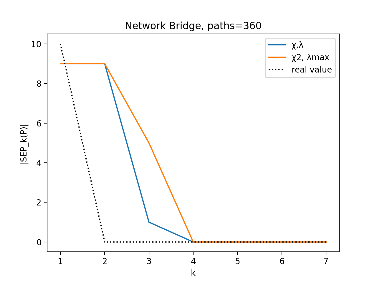

5.1 Experiments
Let . Assume to have a real set of paths over nodes. From we extract the for all and we then estimate as , using the closed formula in Theorem 5.2.
In Figure 2 and 3 we consider two graphs from the Internet topology Zoo (ClaraNet and BTEurope) and we consider set of measurement paths obtained from these networks by taking all the different paths starting in source and ending in a target node (green nodes are source and red nodes are target). In the second table in each Figure ee compare the real values of with the values of for all these paths obtaining results very tight to the real values. Notice that to compute we need to compute for all 11 1 This is because we need to use the for all .. We consider another estimates of obtained from by having only one value for all the ’s. We consider the significant case , where 22 2 It is easy to see that .. Notice that in these cases we do not have to have available all the for all of size at most and the computation can be made much less expensive since and we can use methods to approximate . The estimates is already very good in all these examples.
In each table we also scatter the estimates coming from the MLE method.
6 Complexity of -identifiability and the minimum hitting set
Consider the optimization problem Minimum Hitting Set, , that given an hypergraph (a set-system) , where , asks to find the smallest such that for all , . is a notorious -complete problem [1, 9] extending vertex cover.
We show how to use to find the minimal such that is not - in , i.e. there exits a set of nodes of size , such that .
Theorem 6.1.
Assume is solvable in polynomial time, then, deciding whether is not - in is solvable in polynomial time.
Proof.
Consider the subset of of those nodes touching at least a path in . Let be the vector of dimension defined in the -th coordinate as follows:
has no -coordinate. For otherwise there is a path in only touching . Hence has all -coordinates. We consider the set-system obtained from by restricting the columns to and the rows to . Let be the smallest subset of provided by and covering all . Hence is not -, since .
The optimality of the bound is an immediate consequence of the optimality of . There is no subset of smaller than such that , since of course and, by optimality of , it cannot be smaller than . ∎
The problem of finding a minimal transversal in an hypergraph is a simplification of (see below) which can be decided efficiently. Our reduction hence suggests to implement an algorithm on concrete example of paths where we find the smallest transversal instead of the minimal hitting set.
Let us recall the following definitions from hypergraph transversal problem [4].
Definition 6.2.
Let be an hypergraph. A set is called a transversal of if it meets all the edges of , i.e. if . A transversal is called minimal if no proper subset of is a transversal.
It is possible to find in time a minimal transversal of by the following algorithm (see also [4]). If , then every subset of is a transversal of , hence the minimal one is . If , let . Then define:
Hence is a minimal transversal of . Notice however that it is not necessarily the smallest (by cardinality) transversal of . In fact this last problem is the problem which is -hard.
Let us call be a procedure that implements the previous algorithm on a given , and given an order on , and outputs a minimal transversal of .
The proof of Theorem 6.1 suggests an algorithm to compute an upper bound on the -separablity of a node in , where instead of computing the minimum hitting set we compute a minimal transversal using on any order of the variables.
However we can think of a slightly different algorithm which is computing HT not only once on but several times on a sequence of hypergraphs of decreasing complexity.
Consider the following sets: for all , let , for all and . Let be the set of indices of the . We say that is a -decreasing sequence since, by definition, whenever , and .
The algorithm starts by computing the set and the set of indices of such sets which are not empty. The main observations on the algorithm are the following:
- •
that is a -decreasing sequence. At each step we try to cover only the paths in not already covered before. This is the reason why in line 2 we restrict only to -coordinates in . The vectors are also defined accordingly. Only the coordinates in are important since the rest are already covered by some previous . That is the reason why in line 2 we define to be the vector in all the coordinates not in .
- •
Another observation is that at each step we want to save the minimal set of nodes sufficient to cover all the ’s in . This is the meaning of the call to HT in line 2.
- •
finally, when we have done with analizying all the family of the sets ’s, is covered by the union of the vectors (this is by an argument similar to that fof Theorem 6.1). But it is sufficient to have the minimal subset of this family for covering all . To this end we perform a final call to HT on input the set-system, in 2.
6.1 -Completeness
Consider the following optimization problem MIN-NOT- ().
Input: A Boolean matrix , an element ;
Output: such that is not - and is - for all .
Theorem 6.3.
is -complete
Proof.
To see that is in we can use the reduction in Theorem 6.1 which is in fact proving that . Since [1], then .
To prove the -hardness of we show the opposite reduction, i.e. that . Hence the result follows by the -hardenss of [1]. Let be an instance of . We define an instance of as follows:
- •
The set of nodes of is .
- •
The set of paths of is ;
- •
;
Since a minimal hitting set is touching all edges in , that means that . Hence is not -. Moreover since it is minimal, then for any subset of of size smaller that there is an edge not in . That means that , that is is - in for any .
On the opposite direction, assume that is witnessing that is not - but is - for any , then is clearly a minimal hitting set in .
7 Localizing failure nodes in real networks
In this section we study some heuristics to compute as more precisely as possible the number of -identifiable nodes in set of measurements paths defined on concrete networks, that is the the set of all paths from between monitor nodes. According to Section 4 we study upper bounds on the number of -distinguishable nodes.
To upper bound we lower bound the number of node which are not distinguishable in . In fact we will localize specific sets of nodes which we can guarantee to be not -distinguishable.
Let be given and let . We let be a subset of . This should be meant as (a method to generate) a collection of subset of at most nodes in as function of the node . An example can be: the subsets of made by at most nodes which are at distance at most from . For any , let . This should be meant as (a method to generate) a subset of all paths touching both nodes and .
Definition 7.1.
Let and be given for . We say that and are -equal modulo in if
- 1.
such that , and
- 2.
, .
Let
Lemma 7.2.
For all , .
Proof.
Let we have to find a with such that . Fix as the one in given by the the definition of . We first argue that . By Definition 7.1 case (1) we know that there are such that . Consider a . If , then and hence . If , then and then by Definition 7.1 case (1) and hence in .
Let , then for some . If , then . If , then and then, by Definition 7.1 case (1), . ∎
By Lemma 7.2 nodes in are not -distinguishable and, for the anti-monotonicity, are not -,-,, -distinguishable.
We now study how to upper bound the number of -distinguishable nodes in given a specific definition of and . Consider the following family of vertices in :
Definition 7.3.
Let . .
Theorem 7.4.
.
Proof.
We abbreviate with . First we claim that . This is because for all , if , then , by definition of .
By definition of it follows that , and hence that .
∎
Notice that the proof of the theorem is constructive and is counting well-defined nodes in the network, so that nodes can also precisely be localized.
7.1 Examples of applications
We show how to use previous results to localize and upper bound the number of -identifiable nodes on real set of measurements paths. The estimate will depend on what set we consider for any node and on what set of paths we are going to test path not distinguishability. However once we have fixed and the algorithm we run is always the same and reflects the discussion in the previous subsection (See Algorithm lb-).
Our method can be applied on a network given as a graph once we have decided the set of measurements paths. Every possible way of choosing and is giving a way to count nodes which are no distinguishable. We caton therefore thinking of applying the method restricting for each node the nodes we are checking be not distiguinshable and the effective paths we are going to to consider. We consider here three potential examples. We will add details on experiments and we wilkla dd other cases in the final version of the paper.
7.1.1 Neighbours
For any given , let , where are the neighbours of and consider for all , the of the paths touching both and its neighbours
7.1.2 Nodes at a fixed distance
For any given , let and . For , the of the paths touching both and .
7.1.3 Shortest paths
In this case we consider as set , and for all , is the set of shortest paths from to .
Acknowledgements
The authors would like to thank Navid Talebanfard to point them to the paper [15]. ∎
References
- [1] Ausiello, G., D’Atri, A., and Protasi, M. Structure preserving reductions among convex optimization problems. J. Comput. Syst. Sci. 21, 1 (1980), 136–153.
- [2] Bartolini, N., He, T., Arrigoni, V., Massini, A., Trombetti, F., and Khamfroush, H. On fundamental bounds on failure identifiability by boolean network tomography. IEEE/ACM Trans. Netw. 28, 2 (2020), 588–601.
- [3] Duffield, N. G. Network tomography of binary network performance characteristics. IEEE Trans. Information Theory 52, 12 (2006), 5373–5388.
- [4] Eiter, T., and Gottlob, G. Identifying the minimal transversals of a hypergraph and related problems. SIAM J. Comput. 24, 6 (1995), 1278–1304.
- [5] Frankl, P., and Füredi, Z. Union-free families of sets and equations over field. Journal of Number Theory 23 (1986), 210–218.
- [6] Galesi, N., and Ranjbar, F. Tight bounds for maximal identifiability of failure nodes in boolean network tomography. In 38th IEEE International Conference on Distributed Computing Systems, ICDCS 2018, Vienna, Austria, July 2-6, 2018 (2018), IEEE Computer Society, pp. 212–222.
- [7] Galesi, N., and Ranjbar, F. Tight bounds to localize failure nodes on trees, grids and through embeddings under boolean network tomography. Submitted (2020).
- [8] Galesi, N., Ranjbar, F., and Zito, M. Vertex-connectivity for node failure identification in boolean network tomography. In Algorithms for Sensor Systems - 15th International Symposium on Algorithms and Experiments for Wireless Sensor Networks, ALGOSENSORS 2019, Munich, Germany, September 12-13, 2019, Revised Selected Papers (2019), F. Dressler and C. Scheideler, Eds., vol. 11931 of Lecture Notes in Computer Science, Springer, pp. 79–95.
- [9] Garey, M. R., and Johnson, D. S. Computers and Intractability, A Guide to the Theory of NP-Completeness, 22 ed. W. H. Freeman and Company, New York, 2000.
- [10] Ma, L., He, T., Leung, K. K., Swami, A., and Towsley, D. Inferring link metrics from end-to-end path measurements: Identifiability and monitor placement. IEEE/ACM Trans. Netw. 22, 4 (2014), 1351–1368.
- [11] Ma, L., He, T., Swami, A., Towsley, D., and Leung, K. K. On optimal monitor placement for localizing node failures via network tomography. Perform. Eval. 91 (2015), 16–37.
- [12] Ma, L., He, T., Swami, A., Towsley, D., and Leung, K. K. Network capability in localizing node failures via end-to-end path measurements. IEEE/ACM Trans. Netw. 25, 1 (2017), 434–450.
- [13] Ma, L., He, T., Swami, A., Towsley, D., Leung, K. K., and Lowe, J. Node failure localization via network tomography. In Proceedings of the 2014 Internet Measurement Conference, IMC 2014, Vancouver, BC, Canada, November 5-7, 2014 (2014), C. Williamson, A. Akella, and N. Taft, Eds., ACM, pp. 195–208.
- [14] Ren, W., and Dong, W. Robust network tomography: K-identifiability and monitor assignment. In 35th Annual IEEE International Conference on Computer Communications, INFOCOM 2016, San Francisco, CA, USA, April 10-14, 2016 (2016), IEEE, pp. 1–9.
- [15] Shangguan, C., and Tamo, I. New turán exponents for two extremal hypergraph problems. SIAM Journal on Discrete Mathematics (2020).