跳到论文正文
W Papers独立论文阅读器 arXiv:2101.04272 论文正文 计算阅读时间 · 0%
引用这篇论文根据当前论文元数据生成,正式投稿前建议核对。


License: CC BY 4.0
arXiv:2101.04272v4 [math.SG] 14 Feb 2022

Arboreal models and their stabilityThanks: DA was partially supported by NSF grant DMS-1638352 and the Simons FoundationThanks: YE was partially supported by NSF grant DMS-1807270. Thanks: DN was partially supported by NSF grant DMS-1802373.

Daniel Álvarez-Gavela Address: Department of Mathematics
Massachusetts Institute of Technology
Cambridge, MA, 02139
Email address: dgavela@mit.edu
, Yakov Eliashberg Address: Department of Mathematics
Stanford University
Stanford, CA 94305
Email address: eliash@stanford.edu
and David Nadler Address: Department of Mathematics
University of California, Berkeley
Berkeley, CA 94720-3840
Email address: nadler@math.berkeley.edu
Date: August 11, 2026
Abstract.

This is the first in a series of papers [AGEN19, AGEN20b, AGEN22] by the authors on the arborealization program. The main goal of the paper is the proof of uniqueness of arboreal models, defined as the closure of the class of smooth germs of Lagrangian submanifolds under the operation of taking iterated transverse Liouville cones. The parametric version of the stability result implies that the space of germs of symplectomorphisms that preserve a canonical model is weakly homotopy equivalent to the space of automorphisms of the corresponding signed rooted tree. Hence the local symplectic topology around a canonical model reduces to combinatorics, even parametrically.

1. Introduction

1.1. Main results

This is the first in a series of papers [AGEN19, AGEN20b, AGEN22] by the authors on the arborealization program.

The initial goal of this program is to determine when a Weinstein manifold can be deformed to have an arboreal skeleton, i.e. a skeleton which is a stratified Lagrangian with arboreal singularities. The main results of [AGEN20b] show this can be achieved for polarized Weinstein manifolds, and moreover, the resulting arboreal space determines the ambient Weinstein manifold. The current paper provides essential local results underlying these global developments, as will be discussed below.

The class of arboreal singularities was first defined by the third author in the paper  [N13] for abstract nn-dimensional complexes (without any smooth structure). Their Lagrangian and Legendrian realizations were also exhibited in  [N13] by means of explicit models. In  [St18] and [E18] these models were further decorated by signs. It is important to point out that the definition in  [N13] fixes only the homeomorphism, and not diffeomorphism type of the singularity. While this is sufficient for many applications, for example calculating of some invariants, the homeomorphism type of an arboreal skeleta does not determine in general the symplectomorphism type of the ambient manifold, even if the skeleton is smooth (e.g. see  [Ab12]). On the other hand, it is not even possible to discuss the problem of whether the symplectic topology of the Weinstein manifold is determined by its skeleton before establishing canonical up to symplectomorphism local models of singularities.

We prove in the current paper that the singularities in the class of signed arboreal Lagrangian and Legendrian singularities introduced by Definition 1.1 below are determined up to ambient symplectomorphism by their combinatorial type, and present their canonical models. The uniqueness problem was not even considered in the prior papers on this subject.

We find it surprising that there is a solution to the problem of finding such canonical models. Indeed, we do not know any other sufficiently large classes of Lagrangian singularities which admit a discrete classification up to ambient symplectomorphism. Following Definition 1.1, given a choice of canonical model, if we take its Legendrian lift, apply a contactomorphism taking it into generic position, and then form its Liouville cone, we must once again obtain a canonical model. This is essentially equivalent to the statement that any sufficiently small deformation of a Legendrian model by a contactomorphism of P​T∗​ℝnPT^{*}{\mathbb{R}}^{n} can be realized by an element of a smaller subgroup of contactomorphisms formed by contact lifts of diffeomorphisms of (ℝn,0)({\mathbb{R}}^{n},0).

To discuss this in more detail, we first introduce some auxiliary notions. A closed subset of a symplectic or contact manifold is called isotropic if is stratified by isotropic submanifolds. It is called Lagrangian or Legendrian if it is isotropic and purely of the maximal possible dimension. The germ at the origin of a locally simply-connected isotropic subset L⊂T∗​ℝnL\subset T^{*}{\mathbb{R}}^{n} of the cotangent bundle with its standard Liouville structure λ=p​d​q\lambda=pdq admits a unique lift to an isotropic germ at the origin L^⊂J1​ℝn=T∗​ℝn×ℝ\widehat{L}\subset J^{1}{\mathbb{R}}^{n}=T^{*}{\mathbb{R}}^{n}\times{\mathbb{R}} of the 1-jet bundle. Given an isotropic subset Λ⊂S∗​ℝn\Lambda\subset S^{*}{\mathbb{R}}^{n} of the cosphere bundle, its Liouville cone C⁡(Λ)⊂T∗​ℝC(\Lambda)\subset T^{*}{\mathbb{R}}, i.e. the closure of its saturation by trajectories of the Liouville vector field Z=p​∂∂pZ=p\frac{\partial}{\partial p}, is an isotropic subset.

Definition 1.1.

Arboreal Lagrangian (resp. Legendrian) singularities form the smallest class Arbn𝑠𝑦𝑚𝑝\mathrm{Arb}^{\mathit{symp}}_{n} (resp. Arbn𝑐𝑜𝑛𝑡\mathrm{Arb}^{\mathit{cont}}_{n}) of germs of closed isotropic subsets in 2​n2n-dimensional symplectic (resp. (2​n+1)(2n+1)-dimensional contact) manifolds such that the following properties are satisfied:

  1. (i)

    (Invariance) Arbn𝑠𝑦𝑚𝑝\mathrm{Arb}^{\mathit{symp}}_{n} is invariant with respect to symplectomorphisms and Arbn𝑐𝑜𝑛𝑡\mathrm{Arb}^{\mathit{cont}}_{n} is invariant with respect to contactomorphisms.

  2. (ii)

    (Base case) Arb0𝑠𝑦𝑚𝑝\mathrm{Arb}^{\mathit{symp}}_{0} contains p​t=ℝ0⊂T∗​ℝ0=p​tpt={\mathbb{R}}^{0}\subset T^{*}{\mathbb{R}}^{0}=pt.

  3. (iii)

    (Stabilizations) If L⊂(X,ω)L\subset(X,\omega) is in Arbn𝑠𝑦𝑚𝑝\mathrm{Arb}^{\mathit{symp}}_{n}, then the product L×ℝ⊂(X×T∗​ℝ,ω+d​p∧d​q)L\times{\mathbb{R}}\subset(X\times T^{*}{\mathbb{R}},\omega+dp\wedge dq) is in A​r​bn+1𝑠𝑦𝑚𝑝Arb^{\mathit{symp}}_{n+1}.

  4. (iv)

    (Legendrian lifts) If L⊂T∗​ℝnL\subset T^{*}{\mathbb{R}}^{n} is in Arbn𝑠𝑦𝑚𝑝\mathrm{Arb}^{\mathit{symp}}_{n}, then its Legendrian lift L^⊂J1​ℝn\widehat{L}\subset J^{1}{\mathbb{R}}^{n} is in Arbn𝑐𝑜𝑛𝑡\mathrm{Arb}^{\mathit{cont}}_{n}.

  5. (v)

    (Liouville cones) Let Λ1,…,Λk⊂S∗​ℝn\Lambda_{1},\dots,\Lambda_{k}\subset S^{*}{\mathbb{R}}^{n} be a finite disjoint union of arboreal Legendrian germs from A​r​bn−1𝑐𝑜𝑛𝑡Arb^{\mathit{cont}}_{n-1} centered at points z1,…,zk∈S∗​ℝnz_{1},\dots,z_{k}\in S^{*}{\mathbb{R}}^{n}. Let π:S∗​ℝn→ℝn\pi:S^{*}{\mathbb{R}}^{n}\to{\mathbb{R}}^{n} be the front projection. Suppose

    • -

      π⁡(z1)=⋯=π⁡(zk)\pi(z_{1})=\dots=\pi(z_{k});

    • -

      For any ii, and smooth submanifold Y⊂ΛiY\subset\Lambda_{i}, the restriction π|Y:Y→ℝn\pi|_{Y}:Y\to{\mathbb{R}}^{n} is an embedding (or equivalently, an immersion, since we only consider germs).

    • -

      For any distinct i1,…,iℓi_{1},\ldots,i_{\ell}, and any smooth submanifolds Yi1⊂Λi1,…,Yiℓ⊂ΛiℓY_{i_{1}}\subset\Lambda_{i_{1}},\dots,Y_{i_{\ell}}\subset\Lambda_{i_{\ell}}, the restriction π|Yi1∪⋯∪Yiℓ:Yi1∪⋯∪Yiℓ→ℝn\pi|_{Y_{i_{1}}\cup\dots\cup Y_{i_{\ell}}}:Y_{i_{1}}\cup\dots\cup Y_{i_{\ell}}\to{\mathbb{R}}^{n} is self-transverse.

    Then the union ℝn∪C⁡(Λ1)∪⋯∪C⁡(Λk){\mathbb{R}}^{n}\cup C(\Lambda_{1})\cup\dots\cup C(\Lambda_{k}) of the Liouville cones with the zero-section form an arboreal Lagrangian germ from Arbn𝑠𝑦𝑚𝑝\mathrm{Arb}^{\mathit{symp}}_{n}.

With the above classes defined, we can also allow boundary by additionally taking the product L×ℝ≥0⊂(X×T∗​ℝ,ω+d​p∧d​q)L\times{\mathbb{R}}_{\geq 0}\subset(X\times T^{*}{\mathbb{R}},\omega+dp\land dq) for any arboreal Lagrangian L⊂(X,ω)L\subset(X,\omega), and similarly for arboreal Legendrians.

In Section 3, we prove the Stability Theorem 3.5 for arboreal models as characterized by Definition 1.1. Its main application is the following: for fixed dimension nn, up to ambient symplectomorphism or contactomorphism, Definition 1.1 produces only finitely many local models.

More precisely, to each member of the class Arbn𝑠𝑦𝑚𝑝\mathrm{Arb}^{\mathit{symp}}_{n}, one can assign a signed rooted tree 𝒯^=(T,ρ,ε){\widehat{\mathscr{T}}}=(T,\rho,\varepsilon) with at most n+1n+1 vertices. Here TT is a finite acyclic graph, ρ\rho is a distinguished root vertex, and ε\varepsilon is a sign function on the edges of TT not adjacent to ρ\rho. This discrete data completely determines the germ:

Theorem 1.2.

If two arboreal Lagrangian singularities L⊂(X,ω)L\subset(X,\omega), L′⊂(X′,ω′)L^{\prime}\subset(X^{\prime},\omega^{\prime}) of the class Arbn𝑠𝑦𝑚𝑝\mathrm{Arb}^{\mathit{symp}}_{n} have the same dimension and signed rooted tree 𝒯^{\widehat{\mathscr{T}}}, then there is (the germ of) a symplectomorphism (X,ω)≃(X′,ω′)(X,\omega)\simeq(X^{\prime},\omega^{\prime}) identifying LL and L′L^{\prime}.

Similarly, each member of the class Arbn𝑐𝑜𝑛𝑡\mathrm{Arb}^{\mathit{cont}}_{n} is determined by an associated signed rooted tree 𝒯^=(T,ρ,ε){\widehat{\mathscr{T}}}=(T,\rho,\varepsilon) with at most n+1n+1 vertices.

As a representative for each signed rooted tree 𝒯^{\widehat{\mathscr{T}}}, one may take the local model L𝒯^⊂T∗​ℝnL_{\widehat{\mathscr{T}}}\subset T^{*}{\mathbb{R}}^{n} detailed in Section 2, where n=|n⁡(𝒯^)|n=|n({\widehat{\mathscr{T}}})| is one less than the number of vertices in the tree. The model L𝒯^⊂T∗​ℝnL_{\widehat{\mathscr{T}}}\subset T^{*}{\mathbb{R}}^{n} is given as the positive conormal to an explicit front H𝒯^⊂ℝnH_{\widehat{\mathscr{T}}}\subset{\mathbb{R}}^{n} defined by elementary equations. Our exposition in Section 2 is self-contained and the reader need not be familiar with [N13] or [St18]. In particular, we emphasize the inductive nature of the constructions, and reformulate signs to match inductive arguments to come.

In Section 3, we also establish a parametric version of the Stability Theorem 3.5, whose main consequence can be formulated as follows:

Theorem 1.3.

Fix a signed rooted tree 𝒯^=(T,ρ,ε){\widehat{\mathscr{T}}}=(T,\rho,\varepsilon), set n=|n⁡(𝒯^)|n=|n({\widehat{\mathscr{T}}})| and consider the arboreal 𝒯^{\widehat{\mathscr{T}}}-front H𝒯^⊂ℝnH_{\widehat{\mathscr{T}}}\subset{\mathbb{R}}^{n}. Let D⁡(ℝn,H𝒯^)D({\mathbb{R}}^{n},H_{\widehat{\mathscr{T}}}) be the group of germs at 00 of diffeomorphisms of ℝn{\mathbb{R}}^{n} preserving H𝒯^H_{\widehat{\mathscr{T}}} as a front, i.e.  as a subset along with its coorientation.

Then the fibers of the natural map D⁡(ℝn,H𝒯^)→Aut⁡(𝒯^)D({\mathbb{R}}^{n},H_{\widehat{\mathscr{T}}})\to{\rm Aut}({\widehat{\mathscr{T}}}) are weakly contractible.

Hence, the local symplectic topology of an arboreal singularity is completely characterized by the combinatorics of the underlying signed rooted tree, even parametrically.

We conclude this introduction by briefly explaining the role of Theorem 1.2 within the global results of the arborealization program. It was shown in [N15] that singularities of Whitney stratified Lagrangians can always be locally deformed to arboreal Lagrangians in a non-characteristic fashion, i.e. without changing their microlocal invariants. The question of whether a global theory exists at the level of Weinstein structures is more subtle. In two dimensions the story is classical: generic ribbon graphs provide arboreal skeleta. In four dimensions, Starkston proved in  [St18] that arboreal skeleta always exist in the Weinstein homotopy class of any Weinstein domain.

In the sequel [AGEN20b], we show any polarized Weinstein manifold, i.e. a Weinstein manifold with a global field of Lagrangian planes in its tangent bundle, can be deformed to have an arboreal skeleton. More specifically, the arboreal singularities that arise are positive in the sense that they are indexed by signed rooted trees with all positive signs +1+1, and conversely, any Weinstein manifold with a positive arboreal skeleton comes with a canonical (homotopy class of) polarization.

Now, the arguments of [AGEN20b] produce skeleta with singularities satisfying the characterization of Definition 1.1. So without the uniqueness of Theorem 1.2, we would still be left to study the possible moduli of such singularities: it could happen that two skeleta built with the same combinatorics lead to different Weinstein manifolds. The uniqueness of Theorem 1.2 guarantees this is not the case: there is no moduli of the singularities arising, and indeed their geometry is uniquely specified by the combinatorics. (In fact, the situation is even better: thanks to the arboreal Darboux-Weinstein theorem proved in [AGEN20b], any symplectic thickenings of the skeleton that induce equivalent orientation structures, a further combinatorial decoration on the skeleton, are themselves equivalent.) Thus pairing the results of the current paper with those of [AGEN20b] one is able to express polarized Weinstein manifolds in combinatorial terms. In a forthcoming paper [AGEN22] we will classify all bifurcations (== ”Reidemeister moves”) relating arboreal skeleta of two polarized Weinstein manifolds related by a polarized Weinstein homotopy, thus reducing the problem of classification of (polarized) Weinstein structures up to deformational equivalence to the problem of classification of arboreal complexes up to diffeomorphism and Reidemeister moves.

1.2. Acknowledgements

We are very grateful to Laura Starkston who collaborated with us on the initial stages of this project. The first author is grateful for the great working environment he enjoyed at Princeton University and the Institute for Advanced Study, as well as for the hospitality of the Centre de recherches mathématiques of Montreal. The second author thanks RIMS Kyoto and ITS ETH Zurich for their hospitality. The third author thanks MSRI for its hospitality. Finally, we are very grateful for the support of the American Institute of Mathematics, which hosted a workshop on the arborealization program in 2018 from which this project has greatly benefited.

2. Arboreal models

2.1. Quadratic fronts

Before we present the local models for arboreal singularities, we introduce the quadratic fronts out of which the models will be built and discuss some of their basic properties.

2.1.1. Basic constructions

For i≥0i\geq 0, define functions hi:ℝi→ℝh_{i}:{\mathbb{R}}^{i}\to{\mathbb{R}} by the inductive formula

h0=0\textstyle{h_{0}=0}hi=hi​(x1,…,xi)=x1−hi−1​(x2,…,xi)2\textstyle{h_{i}=h_{i}(x_{1},\ldots,x_{i})=x_{1}-h_{i-1}(x_{2},\ldots,x_{i})^{2}}

For example, for small ii, we have

h1​(x1)=x1\textstyle{h_{1}(x_{1})=x_{1}}h2​(x1,x2)=x1−x22\textstyle{h_{2}(x_{1},x_{2})=x_{1}-x_{2}^{2}}h3​(x1,x2,x3)=x1−(x2−x32)2\textstyle{h_{3}(x_{1},x_{2},x_{3})=x_{1}-(x_{2}-x_{3}^{2})^{2}}

Fix n≥0n\geq 0. For i=0,…,ni=0,\ldots,n, define smooth graphical hypersurfaces

Γin={x0=hi2}⊂ℝn+1\textstyle{{}^{n}\Gamma_{i}=\{x_{0}=h_{i}^{2}\}\subset{\mathbb{R}}^{n+1}}

equipped with the graphical coorientation, and consider their union

Γn=⋃i=0nΓin\textstyle{{}^{n}\Gamma=\bigcup_{i=0}^{n}{}^{n}\Gamma_{i}}

Note the elementary identities

Γin=Γii×ℝn−i\textstyle{{}^{n}\Gamma_{i}={}^{i}\Gamma_{i}\times{\mathbb{R}}^{n-i}}i=0,…,n\textstyle{i=0,\ldots,n}
Γin∩Γ0n=Γi−1n−1\textstyle{{}^{n}\Gamma_{i}\cap{}^{n}\Gamma_{0}={}^{n-1}\Gamma_{i-1}}i=1,…,n\textstyle{i=1,\ldots,n}
Refer to caption
Figure 2.1. The hypersurfaces Γ01{}^{1}\Gamma_{0} (green) and Γ11{}^{1}\Gamma_{1} (blue)
Refer to caption
Figure 2.2. The hypersurfaces Γ02{}^{2}\Gamma_{0} (green), Γ12{}^{2}\Gamma_{1} (red) and Γ22{}^{2}\Gamma_{2} (blue).

Let T∗​ℝnT^{*}{\mathbb{R}}^{n} denote the cotangent bundle with canonical 1-form p​d​x=∑i=1npi​d​xipdx=\sum_{i=1}^{n}p_{i}dx_{i} where p=(p1,…,pn)p=(p_{1},\ldots,p_{n}) are dual coordinates to x=(x1,…,xn)x=(x_{1},\ldots,x_{n}). Let J1​ℝn=ℝ×T∗​ℝnJ^{1}{\mathbb{R}}^{n}={\mathbb{R}}\times T^{*}{\mathbb{R}}^{n} denote the 1-jet bundle with contact form d​x0+p​d​x=d​x0+∑i=1npi​d​xidx_{0}+pdx=dx_{0}+\sum_{i=1}^{n}p_{i}dx_{i}.

Given a function f:ℝn→ℝf:{\mathbb{R}}^{n}\to{\mathbb{R}} with graph Γf={x0=f(x)}⊂ℝ×ℝn\Gamma_{f}=\{x_{0}=f(x)\}\subset{\mathbb{R}}\times{\mathbb{R}}^{n}, we have the conormal Lagrangian of the graph LΓf={x0=f(x),pi=−p0∂f/∂xi}⊂T∗ℝn+1L_{\Gamma_{f}}=\{x_{0}=f(x),\,p_{i}=-p_{0}\partial f/\partial x_{i}\}\subset T^{*}{\mathbb{R}}^{n+1}, and the conormal Legendrian of the graph ΛΓf={x0=f(x),p0=1,pi=−∂f/∂xi}⊂J1ℝn\Lambda_{\Gamma_{f}}=\{x_{0}=f(x),\,p_{0}=1,\,p_{i}=-\partial f/\partial x_{i}\}\subset J^{1}{\mathbb{R}}^{n}.

For i=0i=0, let L0n=ℝn⊂T∗​ℝn{}^{n}L_{0}={\mathbb{R}}^{n}\subset T^{*}{\mathbb{R}}^{n} denote the zero-section. For i=1,…,ni=1,\ldots,n, introduce the conormal Lagrangian

Lin=LΓi−1n−1⊂T∗​ℝn\textstyle{{}^{n}L_{i}=L_{{}^{n-1}\Gamma_{i-1}}\subset T^{*}{\mathbb{R}}^{n}}

of the graph Γi−1n−1⊂ℝn{}^{n-1}\Gamma_{i-1}\subset{\mathbb{R}}^{n}, and consider their union

Ln=⋃i=0nLin\textstyle{{}^{n}L=\bigcup_{i=0}^{n}{}^{n}L_{i}}

Similarly, for i=0,…,ni=0,\ldots,n, introduce the conormal Legendrian

Λin=ΛΓin⊂J1​ℝn\textstyle{{}^{n}\Lambda_{i}=\Lambda_{{}^{n}\Gamma_{i}}\subset J^{1}{\mathbb{R}}^{n}}

of the graph Γin⊂ℝn+1{}^{n}\Gamma_{i}\subset{\mathbb{R}}^{n+1}, and consider their union

Λn=⋃i=0nΛin\textstyle{{}^{n}\Lambda=\bigcup_{i=0}^{n}{}^{n}\Lambda_{i}}

Note that the Liouville form vanishes on the conical Lagrangian Lin⊂T∗​ℝn{}^{n}L_{i}\subset T^{*}{\mathbb{R}}^{n}, hence its lift to J1​ℝn=ℝ×T∗​ℝnJ^{1}{\mathbb{R}}^{n}={\mathbb{R}}\times T^{*}{\mathbb{R}}^{n} with zero primitive is a Legendrian. We have the following compatibility:

Lemma 2.1.

The contactomorphism

S:J1​ℝn\textstyle{S:J^{1}{\mathbb{R}}^{n}\ignorespaces\ignorespaces\ignorespaces\ignorespaces}J1​ℝn\textstyle{J^{1}{\mathbb{R}}^{n}}
S⁡(x0,x,p)=(x0−p12/4,x1+p1/2,x2,…,xn,p1,…,pn)\textstyle{S(x_{0},x,p)=(x_{0}-p_{1}^{2}/4,x_{1}+p_{1}/2,x_{2},\ldots,x_{n},p_{1},\ldots,p_{n})}

takes the Legendrian Λin{}^{n}\Lambda_{i} isomorphically to the Legendrian {0}×Lin\{0\}\times{}^{n}L_{i}, and thus the union Λn{}^{n}\Lambda isomorphically to the union {0}×Ln\{0\}\times{}^{n}L.

Proof.

Set hi,1=hi−1​(x2,…,xi)h_{i,1}=h_{i-1}(x_{2},\ldots,x_{i}) so that hi=x1−hi,12h_{i}=x_{1}-h_{i,1}^{2}. Observe Λin⊂J1​ℝn{}^{n}\Lambda_{i}\subset J^{1}{\mathbb{R}}^{n} is given by the equations

x0=hi2\textstyle{x_{0}=h_{i}^{2}}p​d​x=−d​hi2=−2​hi​d​hi=−2​hi​(d​x1−2​hi,1​d​hi,1)\textstyle{pdx=-dh_{i}^{2}=-2h_{i}dh_{i}=-2h_{i}(dx_{1}-2h_{i,1}dh_{i,1})}

so in particular p1=−2​hip_{1}=-2h_{i} and ∑i=2npi​d​xi=4​hi​hi,1​d​hi,1\sum_{i=2}^{n}p_{i}dx_{i}=4h_{i}h_{i,1}dh_{i,1}.

If we write (x^0,x^,p)=S⁡(x0,x,p)(\hat{x}_{0},\hat{x},p)=S(x_{0},x,p), for (x0,x,p)∈Λin(x_{0},x,p)\in{}^{n}\Lambda_{i}, then we have

x^0=x0−p12/4=±(x0−hi2)=0\textstyle{\hat{x}_{0}=x_{0}-p_{1}^{2}/4=\pm(x_{0}-h_{i}^{2})=0}x^1=x1+p1/2=x1−hi=x1−(x1−hi,12)=hi,12\textstyle{\hat{x}_{1}=x_{1}+p_{1}/2=x_{1}-h_{i}=x_{1}-(x_{1}-h_{i,1}^{2})=h_{i,1}^{2}}

Now it remains to observe Lin⊂T∗​ℝn{}^{n}L_{i}\subset T^{*}{\mathbb{R}}^{n} is given by the equations

x1=hi,12\textstyle{x_{1}=h_{i,1}^{2}}∑i=2npi​d​xi=−p1​d​hi,12=−2​p1​hi,1​d​hi,1\textstyle{\sum_{i=2}^{n}p_{i}dx_{i}=-p_{1}dh^{2}_{i,1}=-2p_{1}h_{i,1}dh_{i,1}}

This completes the proof. ∎

2.1.2. Distinguished quadrants

We now specify some distinguished quadrants of the Γn{}^{n}\Gamma which we will use to define our arboreal models. Which of these quadrants are cut out by our sign conventions will become clearer when the arboreal models are introduced.

For 0≤j<i≤n0\leq j<i\leq n, set

hi,j:=hi−j​(xj+1,…,xi)\textstyle{h_{i,j}:=h_{i-j}(x_{j+1},\ldots,x_{i})}

so in particular hi,0=hi​(x1,…,xi)h_{i,0}=h_{i}(x_{1},\ldots,x_{i}) and hi,i−1=h1​(xi)=xih_{i,i-1}=h_{1}(x_{i})=x_{i}.

For fixed 0≤i≤n0\leq i\leq n, consider the collection of functions

hi,0,…,hi,i−1\textstyle{h_{i,0},\ldots,h_{i,i-1}}

Note the triangular nature of the linear terms of the collection: for all 0≤j≤i−10\leq j\leq i-1, the subcollection

hi,j−xj+1,hi,j+1,…,hi,i−1\textstyle{h_{i,j}-x_{j+1},h_{i,j+1},\ldots,h_{i,i-1}}

is independent of xj+1x_{j+1}. Thus the level sets of the collection are mutually transverse.

Fix once and for all a list of signs δ=(δ0,δ1,…,δn)\delta=(\delta_{0},\delta_{1},\ldots,\delta_{n}), δi∈{±1}\delta_{i}\in\{\pm 1\}. Define the domain quadrant Qiδn⊂ℝn{}^{n}Q^{\delta}_{i}\subset{\mathbb{R}}^{n} to be cut out by the inequalities

δ1​hi,0≤0,…,δi​hi,i−1≤0\textstyle{\delta_{1}h_{i,0}\leq 0,\ldots,\delta_{i}h_{i,i-1}\leq 0}

By the transversality noted above, Qiδn{}^{n}Q^{\delta}_{i} is a submanifold with corners diffeomorphic to ℝ≥0i×ℝn−i{\mathbb{R}}_{\geq 0}^{i}\times{\mathbb{R}}^{n-i}. Its codimension one boundary faces are given by the vanishing of one of the functions hi,jh_{i,j}.

Note Qiδn{}^{n}Q^{\delta}_{i} only depends on the truncated list δ1,…,δi\delta_{1},\ldots,\delta_{i}. In particular, it is independent of δ0\delta_{0} which will enter the constructions next.

Define the cooriented hypersurface Γin|δ⊂ℝn+1{}^{n}\Gamma_{i}|_{\delta}\subset{\mathbb{R}}^{n+1} to be the restricted signed graph

Γin|δ={x0=δ0hi2}|Qiδn\textstyle{{}^{n}\Gamma_{i}|_{\delta}=\{x_{0}=\delta_{0}h_{i}^{2}\}|_{{}^{n}Q^{\delta}_{i}}}

with the graphical coorientation.

Thus Γin|δ{}^{n}\Gamma_{i}|_{\delta} is cut out by the equations

x0=δ0​hi2,\textstyle{x_{0}=\delta_{0}h_{i}^{2},}δ1​hi,0≤0,…,δi​hi,i−1≤0\textstyle{\delta_{1}h_{i,0}\leq 0,\ldots,\delta_{i}h_{i,i-1}\leq 0}

Since Γin|δ{}^{n}\Gamma_{i}|_{\delta} is graphical over Qiδn{}^{n}Q^{\delta}_{i}, it is also a submanifold with corners diffeomorphic to ℝ≥0i×ℝn−i{\mathbb{R}}_{\geq 0}^{i}\times{\mathbb{R}}^{n-i}. Likewise, its codimension one boundary faces are given by the vanishing of one of the functions hi,jh_{i,j}.

Consider as well the union

Γn|δ=⋃i=0nΓin|δ\textstyle{{}^{n}\Gamma|_{\delta}=\bigcup_{i=0}^{n}{}^{n}\Gamma_{i}|_{\delta}}
Remark 2.2.

Note that

Γin=⋃δ,δ0=1Γin|δ\textstyle{{}^{n}\Gamma_{i}=\bigcup_{\delta,\delta_{0}=1}{}^{n}\Gamma_{i}|_{\delta}}Γn=⋃δ,δ0=1Γn|δ\textstyle{{}^{n}\Gamma=\bigcup_{\delta,\delta_{0}=1}{}^{n}\Gamma|_{\delta}}

since x∈Γinx\in{}^{n}\Gamma_{i} implies x∈Γin|δx\in{}^{n}\Gamma_{i}|_{\delta} where for 1≤j≤i1\leq j\leq i, we set δj=−sgn⁡(hi,j​(x))\delta_{j}=-{\rm sgn\,}(h_{i,j}(x)), when hi,j​(x)≠0h_{i,j}(x)\not=0, and choose it arbitrarily otherwise.

Remark 2.3.

Note if we set δ′=(δ0,…,δn−1,−δn)\delta^{\prime}=(\delta_{0},\ldots,\delta_{n-1},-\delta_{n}), then the map ℝn+1→ℝn+1{\mathbb{R}}^{n+1}\to{\mathbb{R}}^{n+1}, (x0,…,xn−1,xn)↦(x0,…,xn−1,−xn)(x_{0},\ldots,x_{n-1},x_{n})\mapsto(x_{0},\ldots,x_{n-1},-x_{n}), takes Γn|δ{}^{n}\Gamma|_{\delta} isomorphically to Γn|δ′{}^{n}\Gamma|_{\delta^{\prime}} as a cooriented hypersurface. Thus we could always set δn=1\delta_{n}=1 and not miss any new geometry.

Note Γin∩{x0<0}{}^{n}\Gamma_{i}\cap\{x_{0}<0\}, hence also Γin|δ∩{δ0x0<0}{}^{n}\Gamma_{i}|_{\delta}\cap\{\delta_{0}x_{0}<0\}, is empty since Γin{}^{n}\Gamma_{i} is the graph of hi2≥0h_{i}^{2}\geq 0.

Lemma 2.4.

Fix δ=(δ0,…,δn)\delta=(\delta_{0},\ldots,\delta_{n}), and set δ′=(δ0​δ1,δ2,…,δn)\delta^{\prime}=(\delta_{0}\delta_{1},\delta_{2},\ldots,\delta_{n}). The homeomorphism

s:δ0​ℝ≥0×ℝn\textstyle{s:\delta_{0}{\mathbb{R}}_{\geq 0}\times{\mathbb{R}}^{n}\ignorespaces\ignorespaces\ignorespaces\ignorespaces}δ0​ℝ≥0×ℝn\textstyle{\delta_{0}{\mathbb{R}}_{\geq 0}\times{\mathbb{R}}^{n}}
s⁡(x0,x1,x2,…,xn)=(x0,δ0​δ1​(x1+δ1​δ0​x0),x2,…,xn)\textstyle{s(x_{0},x_{1},x_{2},\ldots,x_{n})=(x_{0},\delta_{0}\delta_{1}(x_{1}+\delta_{1}\sqrt{\delta_{0}x_{0}}),x_{2},\ldots,x_{n})}

gives a cooriented identification

s(Γin|δ∩{δ0x0≥0})=δ0ℝ≥0×Γi−1n−1|δ′\textstyle{s({}^{n}\Gamma_{i}|_{\delta}\cap\{\delta_{0}x_{0}\geq 0\})=\delta_{0}{\mathbb{R}}_{\geq 0}\times{}^{n-1}\Gamma_{i-1}|_{\delta^{\prime}}}0<i≤n\textstyle{0<i\leq n}
Proof.

Recall Γin|δ{}^{n}\Gamma_{i}|_{\delta} is defined by

x0=δ0​hi2\textstyle{x_{0}=\delta_{0}h_{i}^{2}}δ1​hi,0≤0,…,δi​hi,i−1≤0\textstyle{\delta_{1}h_{i,0}\leq 0,\ldots,\delta_{i}h_{i,i-1}\leq 0}

in particular

x0=δ0​hi2\textstyle{x_{0}=\delta_{0}h_{i}^{2}}δ1​hi,0=δ1​hi≤0\textstyle{\delta_{1}h_{i,0}=\delta_{1}h_{i}\leq 0}

Note the functions hi,1,…,hi,i−1h_{i,1},\ldots,h_{i,i-1} are independent of the coordinates x0,x1x_{0},x_{1}.

When δ0​x0≥0\delta_{0}x_{0}\geq 0 and δ1​hi≤0\delta_{1}h_{i}\leq 0, the equation x0=δ0​hi2x_{0}=\delta_{0}h_{i}^{2} is equivalent to δ0​x0=−δ1​hi\sqrt{\delta_{0}x_{0}}=-\delta_{1}h_{i}. Expanding this in terms of the definitions, we can rewrite this in the form

x1+δ1​δ0​x0=hi−1​(x2,…,xi)2\textstyle{x_{1}+\delta_{1}\sqrt{\delta_{0}x_{0}}=h_{i-1}(x_{2},\ldots,x_{i})^{2}}

Thus since δ0′=δ0​δ1\delta_{0}^{\prime}=\delta_{0}\delta_{1}, we see ss takes Γin|δ∩{δ0x0≥0}{}^{n}\Gamma_{i}|_{\delta}\cap\{\delta_{0}x_{0}\geq 0\} into δ0ℝ≥0×{x1=δ0′hi−12}\delta_{0}{\mathbb{R}}_{\geq 0}\times\{x_{1}=\delta^{\prime}_{0}h_{i-1}^{2}\}.

Moreover, the additional functions hi,1,…,hi,i−1h_{i,1},\ldots,h_{i,i-1} cutting out Γi−1n−1|δ′⊂{x1=δ0′hi−12}{}^{n-1}\Gamma_{i-1}|_{\delta^{\prime}}\subset\{x_{1}=\delta^{\prime}_{0}h_{i-1}^{2}\} pull back to the same functions hi,1,…,hi,i−1h_{i,1},\ldots,h_{i,i-1} cutting out Γin|δ{}^{n}\Gamma_{i}|_{\delta}.

Finally, the coorientations of Γin|δ{}^{n}\Gamma_{i}|_{\delta},Γi−1n−1|δ′{}^{n-1}\Gamma_{i-1}|_{\delta^{\prime}} are positive on respectively ∂x0\partial_{x_{0}}, ∂x1\partial_{x_{1}}. Observe the ∂x1\partial_{x_{1}}-component of s∗∂x0s_{*}\partial_{x_{0}} is in the direction of ∂x1\partial_{x_{1}}, and hence ss gives a cooriented identification. ∎

2.1.3. Alternative presentation

For compatibility with inductive arguments, it is useful to introduce an alternative sign convention and alternative presentation of the local models.

Fix signs ε=(ε0,…,εn)\varepsilon=(\varepsilon_{0},\ldots,\varepsilon_{n}). Consider the involution σε:ℝn→ℝn\sigma_{\varepsilon}:{\mathbb{R}}^{n}\to{\mathbb{R}}^{n} defined by σε​(x1,…,xn)=(ε1​x1,…,εn​xn)\sigma_{\varepsilon}(x_{1},\ldots,x_{n})=(\varepsilon_{1}x_{1},\ldots,\varepsilon_{n}x_{n}).

Define the domain quadrant Riεn⊂ℝn{}^{n}R^{\varepsilon}_{i}\subset{\mathbb{R}}^{n} cut out by the inequalities

ε0​ε1​hi,0∘σε≤0,…,εi−1​εi​hi,i−1∘σε≤0\textstyle{\varepsilon_{0}\varepsilon_{1}h_{i,0}\circ\sigma_{\varepsilon}\leq 0,\ldots,\varepsilon_{i-1}\varepsilon_{i}h_{i,i-1}\circ\sigma_{\varepsilon}\leq 0}

Define the cooriented hypersurface Γεin⊂ℝn+1{}^{n}\Gamma_{i}^{\varepsilon}\subset{\mathbb{R}}^{n+1} to be the restricted signed graph

Γiεn={x0=ε0hi2∘σε}|Riεn\textstyle{{}^{n}\Gamma_{i}^{\varepsilon}=\{x_{0}=\varepsilon_{0}h_{i}^{2}\circ\sigma_{\varepsilon}\}|_{{}^{n}R^{\varepsilon}_{i}}}

with the graphical coorientation. Thus Γεin{}^{n}\Gamma_{i}^{\varepsilon} is cut out by the equations

x0=ε0​hi2∘σε\textstyle{x_{0}=\varepsilon_{0}h_{i}^{2}\circ\sigma_{\varepsilon}}ε0​ε1​hi,0∘σε≤0,…,εi−1​εi​hi,i−1∘σε≤0\textstyle{\varepsilon_{0}\varepsilon_{1}h_{i,0}\circ\sigma_{\varepsilon}\leq 0,\ldots,\varepsilon_{i-1}\varepsilon_{i}h_{i,i-1}\circ\sigma_{\varepsilon}\leq 0}

Consider as well the union

Γεn=⋃i=0nΓiεn\textstyle{{}^{n}\Gamma^{\varepsilon}=\bigcup_{i=0}^{n}{}^{n}\Gamma^{\varepsilon}_{i}}
Remark 2.5.

A simple but important observation: Γεin{}^{n}\Gamma_{i}^{\varepsilon} in fact only depends on ε0,…,εi−1\varepsilon_{0},\ldots,\varepsilon_{i-1} and not εi\varepsilon_{i}. This is because hi,i−1=xih_{i,i-1}=x_{i} and so εi−1​εi​hi,i−1∘σε=εi−1​xi\varepsilon_{i-1}\varepsilon_{i}h_{i,i-1}\circ\sigma_{\varepsilon}=\varepsilon_{i-1}x_{i}. In particular, the union Γεn{}^{n}\Gamma^{\varepsilon} is independent of εn\varepsilon_{n}.

We have the following adaption of Lemma 2.4.

Lemma 2.6.

Fix ε=(ε0,…,εn)\varepsilon=(\varepsilon_{0},\ldots,\varepsilon_{n}), and set ε′=(ε1,…,εn)\varepsilon^{\prime}=(\varepsilon_{1},\ldots,\varepsilon_{n}). The homeomorphism

s:ε0​ℝ≥0×ℝn\textstyle{s:\varepsilon_{0}{\mathbb{R}}_{\geq 0}\times{\mathbb{R}}^{n}\ignorespaces\ignorespaces\ignorespaces\ignorespaces}ε0​ℝ≥0×ℝn\textstyle{\varepsilon_{0}{\mathbb{R}}_{\geq 0}\times{\mathbb{R}}^{n}}
s⁡(x0,x1,x2,…,xn)=(x0,x1+ε0​ε0​x0,x2,…,xn)\textstyle{s(x_{0},x_{1},x_{2},\ldots,x_{n})=(x_{0},x_{1}+\varepsilon_{0}\sqrt{\varepsilon_{0}x_{0}},x_{2},\ldots,x_{n})}

gives a cooriented identification

s(Γiεn∩{ε0x0≥0})=ε0ℝ≥0×Γi−1ε′n−1\textstyle{s({}^{n}\Gamma^{\varepsilon}_{i}\cap\{\varepsilon_{0}x_{0}\geq 0\})=\varepsilon_{0}{\mathbb{R}}_{\geq 0}\times{}^{n-1}\Gamma_{i-1}^{\varepsilon^{\prime}}}0<i≤n\textstyle{0<i\leq n}
Proof.

Recall Γiεn{}^{n}\Gamma^{\varepsilon}_{i} is defined by

x0=ε0​hi2∘σε\textstyle{x_{0}=\varepsilon_{0}h_{i}^{2}\circ\sigma_{\varepsilon}}ε0​ε1​hi,0∘σε≤0,…,εi−1​εi​hi,i−1∘σε≤0\textstyle{\varepsilon_{0}\varepsilon_{1}h_{i,0}\circ\sigma_{\varepsilon}\leq 0,\ldots,\varepsilon_{i-1}\varepsilon_{i}h_{i,i-1}\circ\sigma_{\varepsilon}\leq 0}

in particular

x0=ε0​hi2∘σε\textstyle{x_{0}=\varepsilon_{0}h_{i}^{2}\circ\sigma_{\varepsilon}}ε0​ε1​hi,0∘σε=ε0​ε1​hi∘σε≤0\textstyle{\varepsilon_{0}\varepsilon_{1}h_{i,0}\circ\sigma_{\varepsilon}=\varepsilon_{0}\varepsilon_{1}h_{i}\circ\sigma_{\varepsilon}\leq 0}

Note the functions hi,1,…,hi,i−1h_{i,1},\ldots,h_{i,i-1} are independent of the coordinates x0,x1x_{0},x_{1}.

When ε0​x0≥0\varepsilon_{0}x_{0}\geq 0 and ε0​ε1​hi∘σε≤0\varepsilon_{0}\varepsilon_{1}h_{i}\circ\sigma_{\varepsilon}\leq 0, the equation x0=ε0​hi2∘σεx_{0}=\varepsilon_{0}h_{i}^{2}\circ\sigma_{\varepsilon} is equivalent to ε0​x0=−ε0ε1hi∘σε\sqrt{\varepsilon_{0}x_{0}}=-\varepsilon_{0}\varepsilon_{1}h_{i}\circ\sigma_{\varepsilon}. Expanding this in terms of the definitions, we can rewrite this in the form

x1+ε0​ε0​x0=ε1​hi−1,12∘σε′\textstyle{x_{1}+\varepsilon_{0}\sqrt{\varepsilon_{0}x_{0}}=\varepsilon_{1}h_{i-1,1}^{2}\circ\sigma_{\varepsilon^{\prime}}}

Thus we see ss takes Γiεn∩{ε0x0≥0}{}^{n}\Gamma^{\varepsilon}_{i}\cap\{\varepsilon_{0}x_{0}\geq 0\} into ε0ℝ≥0×{x1=ε1hi−1,12∘σε′}\varepsilon_{0}{\mathbb{R}}_{\geq 0}\times\{x_{1}=\varepsilon_{1}h_{i-1,1}^{2}\circ\sigma_{\varepsilon^{\prime}}\}.

Moreover, the additional functions hi,1,…,hi,i−1h_{i,1},\ldots,h_{i,i-1} cutting out

Γi−1ε′n−1⊂{x1=ε1hi−1,12∘σε′}{}^{n-1}\Gamma_{i-1}^{\varepsilon^{\prime}}\subset\{x_{1}=\varepsilon_{1}h_{i-1,1}^{2}\circ\sigma_{\varepsilon^{\prime}}\}

pull back to the same functions hi,1,…,hi,i−1h_{i,1},\ldots,h_{i,i-1} cutting out Γiεn{}^{n}\Gamma^{\varepsilon}_{i}.

Finally, the coorientations of Γiεn{}^{n}\Gamma^{\varepsilon}_{i},Γε′i−1n−1{}^{n-1}\Gamma_{i-1}^{\varepsilon^{\prime}} are positive on respectively ∂x0\partial_{x_{0}}, ∂x1\partial_{x_{1}}. Observe the ∂x1\partial_{x_{1}}-component of s∗∂x0s_{*}\partial_{x_{0}} is in the direction of ∂x1\partial_{x_{1}}, and hence ss gives a cooriented identification. ∎

Here is a useful corollary that “explains” the geometric meaning of the signs ε\varepsilon.

Corollary 2.7.

Fix ε=(ε0,…,εn)\varepsilon=(\varepsilon_{0},\ldots,\varepsilon_{n}).

For i=0,…,n−1i=0,\ldots,n-1, we have εi=±1\varepsilon_{i}=\pm 1 if and only if Γi+1n{}^{n}\Gamma_{i+1} is on the ±\pm-side of Γin{}^{n}\Gamma_{i} with respect to the graphical d​x0dx_{0}-coorientation.

Moreover, for i=1,…,n−1i=1,\ldots,n-1, we have εi=±1\varepsilon_{i}=\pm 1 if and only if Γi+1n∩Γ0n{}^{n}\Gamma_{i+1}\cap{}^{n}\Gamma_{0} is on the ±\pm-side of Γin∩Γ0n{}^{n}\Gamma_{i}\cap{}^{n}\Gamma_{0} with respect to the graphical d​x1dx_{1}-coorientation.

Proof.

For i=0i=0, the first assertion is immediate from the definitions Γ0n={x0=0}{}^{n}\Gamma_{0}=\{x_{0}=0\} and Γ1n={x0=ε0(ε1x1)2=ε0x12,ε0ε1(ε1x1)=ε0x1≤0}{}^{n}\Gamma_{1}=\{x_{0}=\varepsilon_{0}(\varepsilon_{1}x_{1})^{2}=\varepsilon_{0}x_{1}^{2},\varepsilon_{0}\varepsilon_{1}(\varepsilon_{1}x_{1})=\varepsilon_{0}x_{1}\leq 0\}.

For i>0i>0, both assertions follow by induction from Lemma 2.6. ∎

Fix signs ε=(ε0,…,εn−1)\varepsilon=(\varepsilon_{0},\ldots,\varepsilon_{n-1}). For i=0i=0, let L0εn=ℝn⊂T∗​ℝn{}^{n}L^{\varepsilon}_{0}={\mathbb{R}}^{n}\subset T^{*}{\mathbb{R}}^{n} denote the zero-section. For i=1,…,ni=1,\ldots,n, introduce the positive conormal bundles

Liεn=TΓi−1εn−1+​ℝn⊂T∗​ℝn\textstyle{{}^{n}L^{\varepsilon}_{i}=T^{+}_{{}^{n-1}\Gamma^{\varepsilon}_{i-1}}{\mathbb{R}}^{n}\subset T^{*}{\mathbb{R}}^{n}}

determined by the graphical coorientation, and consider their union

Lεn=⋃i=0nLiεn\textstyle{{}^{n}L^{\varepsilon}=\bigcup_{i=0}^{n}{}^{n}L^{\varepsilon}_{i}}

Fix signs ε=(ε0,…,εn)\varepsilon=(\varepsilon_{0},\ldots,\varepsilon_{n}). For i=0,…,ni=0,\ldots,n, introduce the Legendrian

Λiεn⊂J1​ℝn\textstyle{{}^{n}\Lambda^{\varepsilon}_{i}\subset J^{1}{\mathbb{R}}^{n}}

projecting diffeomorphically to the front Γiεn⊂ℝn+1{}^{n}\Gamma^{\varepsilon}_{i}\subset{\mathbb{R}}^{n+1}, and consider their union

Λεn=⋃i=0nΛiεn\textstyle{{}^{n}\Lambda^{\varepsilon}=\bigcup_{i=0}^{n}{}^{n}\Lambda^{\varepsilon}_{i}}

We have the following compatibility of the above Lagrangians and Legendrians analogous to Lemma 2.1.

Lemma 2.8.

Fix signs ε=(ε0,…,εn)\varepsilon=(\varepsilon_{0},\ldots,\varepsilon_{n}), and set ε′=(ε1,…,εn)\varepsilon^{\prime}=(\varepsilon_{1},\ldots,\varepsilon_{n}). The contactomorphism

Sε0:J1​ℝn\textstyle{S_{\varepsilon_{0}}:J^{1}{\mathbb{R}}^{n}\ignorespaces\ignorespaces\ignorespaces\ignorespaces}J1​ℝn\textstyle{J^{1}{\mathbb{R}}^{n}}
Sε0​(x0,x,p)=(x0−ε0​p12/4,x1+ε0​p1/2,x2,…,xn,p1,…,pn)\textstyle{S_{\varepsilon_{0}}(x_{0},x,p)=(x_{0}-\varepsilon_{0}p_{1}^{2}/4,x_{1}+\varepsilon_{0}p_{1}/2,x_{2},\ldots,x_{n},p_{1},\ldots,p_{n})}

takes the Legendrian Λiεn{}^{n}\Lambda^{\varepsilon}_{i} isomorphically to the Legendrian {0}×Liε′n\{0\}\times{}^{n}L^{\varepsilon^{\prime}}_{i}, and thus the union Λεn{}^{n}\Lambda^{\varepsilon} isomorphically to the union {0}×Lε′n\{0\}\times{}^{n}L^{\varepsilon^{\prime}}.

Proof.

The proof is the same as that of Lemma 2.1 with the following observations. Consider the additional equations

ε0​ε1​δ1​hi,0∘σδ≤0,…,εi−1​εi​hi,i−1∘σε≤0\textstyle{\varepsilon_{0}\varepsilon_{1}\delta_{1}h_{i,0}\circ\sigma_{\delta}\leq 0,\ldots,\varepsilon_{i-1}\varepsilon_{i}h_{i,i-1}\circ\sigma_{\varepsilon}\leq 0}

First, over ε0​ε1​hi,0∘σε≤0\varepsilon_{0}\varepsilon_{1}h_{i,0}\circ\sigma_{\varepsilon}\leq 0, when p1=−2ε0ε1hi,0∘σεp_{1}=-2\varepsilon_{0}\varepsilon_{1}h_{i,0}\circ\sigma_{\varepsilon}, we then have p1=−2ε0ε1hi,0∘σε≥0p_{1}=-2\varepsilon_{0}\varepsilon_{1}h_{i,0}\circ\sigma_{\varepsilon}\geq 0, so we obtain the positive conormal direction. Second, the remaining functions hi,1,…,hi,i−1h_{i,1},\ldots,h_{i,i-1} are independent of x0,x1x_{0},x_{1}. Thus Sε0S_{\varepsilon_{0}} indeed takes Λiεn{}^{n}\Lambda^{\varepsilon}_{i} to {0}×Liεn\{0\}\times{}^{n}L^{\varepsilon}_{i}. ∎

Remark 2.9.

By the lemma, we see the Legendrian Λiεn⊂J1​ℝn{}^{n}\Lambda^{\varepsilon}_{i}\subset J^{1}{\mathbb{R}}^{n} is independent of the initial sign ε0\varepsilon_{0} so only depends on ε′=(ε1,…,εn)\varepsilon^{\prime}=(\varepsilon_{1},\ldots,\varepsilon_{n}).

It is also useful to record the following relationship of Γεn{}^{n}\Gamma^{\varepsilon} with the extended model Γn{}^{n}\Gamma.

Lemma 2.10.

Fix signs ε=(ε0,…,εn)\varepsilon=(\varepsilon_{0},\ldots,\varepsilon_{n}).

Given a contactomorphism J1​ℝn→J1​ℝnJ^{1}{\mathbb{R}}^{n}\to J^{1}{\mathbb{R}}^{n} restricting to a closed embedding Λεn⊂ε0⋅Λn{}^{n}\Lambda^{\varepsilon}\subset\varepsilon_{0}\cdot{}^{n}\Lambda with Λεin⊂ε0⋅Λin{}^{n}\Lambda_{i}^{\varepsilon}\subset\varepsilon_{0}\cdot{}^{n}\Lambda_{i}, for all ii, consider the front Υ=π⁡(Λεn)⊂ε0⋅Γn\Upsilon=\pi({}^{n}\Lambda^{\varepsilon})\subset\varepsilon_{0}\cdot{}^{n}\Gamma.

Then either the involution σε\sigma_{\varepsilon} or its composition with xn↦±xnx_{n}\mapsto\pm x_{n} takes Υ\Upsilon to Γεn{}^{n}\Gamma^{\varepsilon}.

Proof.

Note we have Λ0εn=ε0⋅Λ0n=Λ0n{}^{n}\Lambda^{\varepsilon}_{0}=\varepsilon_{0}\cdot{}^{n}\Lambda_{0}={}^{n}\Lambda_{0}. Consider the intersection Υ′=π⁡((Λεn∖Λ0n)∩Λ0n)\Upsilon^{\prime}=\pi(({}^{n}\Lambda^{\varepsilon}\setminus{}^{n}\Lambda_{0})\cap{}^{n}\Lambda_{0}) as a front inside of π(Λ0n)=Γ0n={x0=0}\pi({}^{n}\Lambda_{0})={}^{n}\Gamma_{0}=\{x_{0}=0\}. By induction, either the involution σε\sigma_{\varepsilon} or its composition with xn↦±xnx_{n}\mapsto\pm x_{n} takes Υ′\Upsilon^{\prime} to Γε′n−1{}^{n-1}\Gamma^{\varepsilon^{\prime}} where ε′=(ε1,…,εn)\varepsilon^{\prime}=(\varepsilon_{1},\ldots,\varepsilon_{n}). So we may assume Υ′=Γε′n−1\Upsilon^{\prime}={}^{n-1}\Gamma^{\varepsilon^{\prime}}. Now observe Γεn{}^{n}\Gamma^{\varepsilon} is the unique way to extend Γε′n−1{}^{n-1}\Gamma^{\varepsilon^{\prime}} within σε​(ε0⋅Γn)\sigma_{\varepsilon}(\varepsilon_{0}\cdot{}^{n}\Gamma) compatible with coorientations. ∎

We also have the following observation about signs. See Section 3.1 for notation.

Lemma 2.11.

Let ν0\nu_{0} be the vertical polarization of T∗​ℝn→ℝnT^{*}{\mathbb{R}}^{n}\to{\mathbb{R}}^{n}.

Then we have ε⁡(ν0,L1εn,L2εn)=ε0\varepsilon(\nu_{0},{}^{n}L^{\varepsilon}_{1},{}^{n}L^{\varepsilon}_{2})=\varepsilon_{0}.

Proof.

Recall L1εn{}^{n}L^{\varepsilon}_{1} is the positive conormal to the graph Γ0εn−1={x0=0}{}^{n-1}\Gamma^{\varepsilon}_{0}=\{x_{0}=0\}, and L1εn{}^{n}L^{\varepsilon}_{1} is the positive conormal to the graph Γ1εn−1={x0=ϵ0x12}{}^{n-1}\Gamma^{\varepsilon}_{1}=\{x_{0}=\epsilon_{0}x_{1}^{2}\}. Since ε0​x12\varepsilon_{0}x_{1}^{2} is an ε0\varepsilon_{0}-definite quadratic form in x1x_{1}, the assertion follows. ∎

2.2. Arboreal models

We now present the local models for arboreal singularities.

2.2.1. Signed rooted trees

Definition 2.12.

We will use the following terminology throughout:

  1. (i)

    A tree TT is a nonempty, finite, connected acyclic graph.

  2. (ii)

    A rooted tree 𝒯=(T,ρ)\mathscr{T}=(T,\rho) is a pair of a tree TT and a distinguished vertex ρ\rho called the root.

  3. (iii)

    A signed rooted tree 𝒯^=(T,ρ,ε){\widehat{\mathscr{T}}}=(T,\rho,\varepsilon) is a rooted tree (T,ρ)(T,\rho) and a decoration ε\varepsilon of a sign ±1\pm 1 on each edge of TT not adjacent to the root ρ\rho.

Refer to caption
Figure 2.3. A signed rooted tree.

Given a signed rooted tree 𝒯^=(T,ρ,ε){\widehat{\mathscr{T}}}=(T,\rho,\varepsilon), we write v⁡(T)v(T) for the set of vertices, e⁡(T)e(T) for the set of edges, and n⁡(𝒯^)=v⁡(T)∖ρn({\widehat{\mathscr{T}}})=v(T)\setminus\rho for the set of non-root vertices. We regard v⁡(T)v(T) as a poset with unique minimum ρ\rho, and in general α≤β∈v⁡(T)\alpha\leq\beta\in v(T) when the shortest path connecting β\beta and ρ\rho contains α\alpha. We call a non-root vertex β\beta a leaf if exactly one edge of TT is adjacent to β\beta, and write ℓ⁡(𝒯^)⊂v⁡(T)\ell({\widehat{\mathscr{T}}})\subset v(T) for the set of leaf vertices.

Remark 2.13.

Throughout what follows, for a finite set SS, we write ℝS{\mathbb{R}}^{S} for the Euclidean space of SS-tuples of real numbers. One may always fix a bijection S≃{1,2,…,n}S\simeq\{1,2,\ldots,n\}, for some n≥0n\geq 0, and hence an isomorphism ℝS≃ℝn{\mathbb{R}}^{S}\simeq{\mathbb{R}}^{n}, but it will be convenient to avoid choosing such identifications when awkward. We will most often consider S=n⁡(𝒯^)S=n({\widehat{\mathscr{T}}}) the non-root vertices for some rooted tree 𝒯^=(T,ρ){\widehat{\mathscr{T}}}=(T,\rho). Here if one prefers to fix a bijection b:n⁡(𝒯^)→∼{1,2,…,|n⁡(𝒯^)|}b:n({\widehat{\mathscr{T}}})\stackrel{{\scriptstyle\sim}}{{\to}}\{1,2,\ldots,|n({\widehat{\mathscr{T}}})|\}, we recommend choosing bb to be order-preserving: if α≤β\alpha\leq\beta, then one should ensure b⁡(α)≤b⁡(β)b(\alpha)\leq b(\beta). This will allow for a clear translation of our constructions.

Definition 2.14.

A signed rooted tree 𝒯^=(T,ρ,ε){\widehat{\mathscr{T}}}=(T,\rho,\varepsilon) is called positive if the decoration ε\varepsilon consists of signs +1+1.

We will associate to any signed rooted tree 𝒯^=(T,ρ,ε){\widehat{\mathscr{T}}}=(T,\rho,\varepsilon), a multi-cooriented hypersurface, conic Lagrangian, and Legendrian

H𝒯^⊂ℝn⁡(𝒯^)\textstyle{H_{\widehat{\mathscr{T}}}\subset{\mathbb{R}}^{n({\widehat{\mathscr{T}}})}}L𝒯^⊂T∗​ℝn⁡(𝒯^)\textstyle{L_{\widehat{\mathscr{T}}}\subset T^{*}{\mathbb{R}}^{n({\widehat{\mathscr{T}}})}}Λ𝒯^⊂J1​ℝn⁡(𝒯^)\textstyle{\Lambda_{\widehat{\mathscr{T}}}\subset J^{1}{\mathbb{R}}^{n({\widehat{\mathscr{T}}})}}

where as usual we write n⁡(𝒯^)=v⁡(T)∖ρn({\widehat{\mathscr{T}}})=v(T)\setminus\rho for the set of non-root vertices.

By definition, the latter two will be determined by the first as follows:

  1. (i)

    L𝒯^L_{\widehat{\mathscr{T}}} is the union of the zero-section ℝn⁡(𝒯^){\mathbb{R}}^{n({\widehat{\mathscr{T}}})} and the positive conormal to H𝒯^H_{\widehat{\mathscr{T}}}.

  2. (ii)

    Λ𝒯^\Lambda_{{\widehat{\mathscr{T}}}} is the Legendrian lift of L𝒯^L_{\widehat{\mathscr{T}}} with zero primitive.

2.2.2. Type AA trees

Let us first consider the distinguished case of An+1A_{n+1}-trees with extremal root.

Definition 2.15.

For n≥0n\geq 0, a linear signed An+1A_{n+1}-rooted tree is a signed rooted tree 𝒜n+1=(An+1,ρ,a)\mathcal{A}_{n+1}=(A_{n+1},\rho,a) with vertices v⁡(An+1)={0,1,…,n}v(A_{n+1})=\{0,1,\ldots,n\}, edges v(An+1)={[i,i+1]|i=0,…,n−1}v(A_{n+1})=\{[i,i+1]\,|\,i=0,\ldots,n-1\}, and root ρ=0\rho=0.

By definition, the sign aa is a length n−1n-1 list of signs (a[1,2],…,a[n−1,n])(a_{[1,2]},\ldots,a_{[n-1,n]}). Let us set ε=(ε0,…,εn−1)=(a[1,2],…,a[n−1,n],1)\varepsilon=(\varepsilon_{0},\ldots,\varepsilon_{n-1})=(a_{[1,2]},\ldots,a_{[n-1,n]},1) to be the length nn list of signs where we pad aa by adding a single 11 at the end.

Definition 2.16.

The models for AnA_{n}-type arboreal singularities are given as follows:

  1. (i)

    The arboreal 𝒜1\mathcal{A}_{1}-front is the empty set H𝒜1=∅H_{\mathcal{A}_{1}}=\emptyset inside the point ℝ0{\mathbb{R}}^{0}.

    For n≥1n\geq 1, the arboreal 𝒜n+1\mathcal{A}_{n+1}-front is the cooriented hypersurface

    H𝒜n+1=Γεn−1⊂ℝn\textstyle{H_{\mathcal{A}_{n+1}}={}^{n-1}\Gamma^{\varepsilon}\subset{\mathbb{R}}^{n}}

    introduced in Section 2.1.3.

  2. (ii)

    For n≥0n\geq 0, the arboreal 𝒜n+1\mathcal{A}_{n+1}-Lagrangian is the union of the zero-section and positive conormal

    L𝒜n+1=ℝn∪Tℝn+​H𝒜n+1⊂T∗​ℝn\textstyle{L_{\mathcal{A}_{n+1}}={\mathbb{R}}^{n}\cup T^{+}_{{\mathbb{R}}^{n}}H_{\mathcal{A}_{n+1}}\subset T^{*}{\mathbb{R}}^{n}}
  3. (iii)

    For n≥0n\geq 0, the arboreal 𝒜n+1\mathcal{A}_{n+1}-Legendrian is the lift

    Λ𝒜n+1={0}×L𝒜n+1⊂J1​ℝn\textstyle{\Lambda_{\mathcal{A}_{n+1}}=\{0\}\times L_{\mathcal{A}_{n+1}}\subset J^{1}{\mathbb{R}}^{n}}
Refer to caption
Figure 2.4. The two A3A_{3} fronts with positive and negative sign.
Refer to caption
Figure 2.5. Two A4A_{4} fronts with different choices of signs. The other two fronts can be obtained from these two by reflections.
Remark 2.17.

Following Remark 2.5, the arbitrary choice of the last sign εn−1=1\varepsilon_{n-1}=1 does not affect the arboreal 𝒜n+1\mathcal{A}_{n+1}-models.

Recall the linear signed An+1A_{n+1}-rooted tree 𝒜n+1=(An+1,ρ,a)\mathcal{A}_{n+1}=(A_{n+1},\rho,a) has vertices v⁡(An+1)={0,1,…,n}v(A_{n+1})=\{0,1,\ldots,n\} with root ρ=0\rho=0, and so the non-root vertices form the set n⁡(𝒜n+1)={1,…,n}n(\mathcal{A}_{n+1})=\{1,\ldots,n\}. In the above definition, we should more invariantly view the ambient Euclidean space ℝn{\mathbb{R}}^{n} in the form ℝn⁡(𝒜n+1){\mathbb{R}}^{n(\mathcal{A}_{n+1})} where the ordering of the coordinates matches that of n⁡(𝒜n+1)n(\mathcal{A}_{n+1}).

With this viewpoint, we rename the smooth pieces of the 𝒜n+1\mathcal{A}_{n+1}-front, indexing them by non-root vertices

Hi=Pi−1εn−1⊂H𝒜n+1\textstyle{H_{i}={}^{n-1}P^{\varepsilon}_{i-1}\subset H_{\mathcal{A}_{n+1}}}i∈n⁡(𝒜n+1)={1,…,n}\textstyle{i\in n(\mathcal{A}_{n+1})=\{1,\ldots,n\}}

Likewise, we rename the smooth pieces of the of the 𝒜n+1\mathcal{A}_{n+1}-Lagrangian, indexing them by vertices

L0=ℝn⊂L𝒜n+1\textstyle{L_{0}={\mathbb{R}}^{n}\subset L_{\mathcal{A}_{n+1}}}
Li=Tℝn+​Hi⊂L𝒜n+1\textstyle{L_{i}=T^{+}_{{\mathbb{R}}^{n}}H_{i}\subset L_{\mathcal{A}_{n+1}}}i∈n⁡(𝒜n+1)={1,…,n}\textstyle{i\in n(\mathcal{A}_{n+1})=\{1,\ldots,n\}}

and similarly, we rename the smooth pieces of the of the 𝒜n+1\mathcal{A}_{n+1}-Legendrian, indexing them by vertices

Λi={0}×L𝒜n+1,i⊂Λ𝒜n+1\textstyle{\Lambda_{i}=\{0\}\times L_{\mathcal{A}_{n+1},i}\subset\Lambda_{\mathcal{A}_{n+1}}}i∈v⁡(𝒜n+1)={0,1,…,n}\textstyle{i\in v(\mathcal{A}_{n+1})=\{0,1,\ldots,n\}}
Lemma 2.18.

For n≥1n\geq 1, and n∈v⁡(An+1)={0,1,…,n}n\in v(A_{n+1})=\{0,1,\ldots,n\} the unique leaf vertex, and H̊n⊂H𝒜n+1\mathring{H}_{n}\subset H_{\mathcal{A}_{n+1}} the interior of the corresponding smooth piece, we have

H𝒜n+1∖H̊n=H𝒜n×ℝ\textstyle{H_{\mathcal{A}_{n+1}}\setminus\mathring{H}_{n}=H_{\mathcal{A}_{n}}\times{\mathbb{R}}}

inside of ℝn⁡(𝒜n+1)=ℝn⁡(𝒜n)×ℝ{\mathbb{R}}^{n(\mathcal{A}_{n+1})}={\mathbb{R}}^{n(\mathcal{A}_{n})}\times{\mathbb{R}}.

Proof.

Recall the other smooth pieces Hi=Pi−1εn−1H_{i}={}^{n-1}P^{\varepsilon}_{i-1}, for i=1,…,n−1i=1,\ldots,n-1, are independent of the last coordinate xnx_{n}. ∎

2.2.3. General trees

Now we consider a general signed rooted tree 𝒯^=(T,ρ,ε){\widehat{\mathscr{T}}}=(T,\rho,\varepsilon).

To each leaf β∈ℓ⁡(𝒯^)\beta\in\ell({\widehat{\mathscr{T}}}), we associate the linear signed An+1A_{n+1}-rooted tree 𝒜β=(Aβ,ρ,a)\mathcal{A}_{\beta}=(A_{\beta},\rho,a) where AβA_{\beta} is the full subtree of TT on the vertices v(Aβ)={α≤β∈v(T)}v(A_{\beta})=\{\alpha\leq\beta\in v(T)\}, and aa is the restricted sign decoration.

Consider the Euclidean space ℝn⁡(𝒯^){\mathbb{R}}^{n({\widehat{\mathscr{T}}})}. For each β∈ℓ⁡(𝒯^)\beta\in\ell({\widehat{\mathscr{T}}}), the inclusion n⁡(𝒜β)⊂n⁡(𝒯^)n(\mathcal{A}_{\beta})\subset n({\widehat{\mathscr{T}}}) induces a natural projection

πβ:ℝn⁡(𝒯^)\textstyle{\pi_{\beta}:{\mathbb{R}}^{n({\widehat{\mathscr{T}}})}\ignorespaces\ignorespaces\ignorespaces\ignorespaces}ℝn⁡(𝒜β)\textstyle{{\mathbb{R}}^{n(\mathcal{A}_{\beta})}}
Definition 2.19.

Let 𝒯^=(T,ρ,ε){\widehat{\mathscr{T}}}=(T,\rho,\varepsilon) be a signed rooted tree.

  1. (i)

    The arboreal model 𝒯^{\widehat{\mathscr{T}}}-front is the multi-cooriented hypersurface given by the union

    H𝒯^=⋃β∈ℓ⁡(𝒯^)πβ−1​(H𝒜β)⊂ℝn⁡(𝒯^)\textstyle{H_{{\widehat{\mathscr{T}}}}=\bigcup_{\beta\in\ell({\widehat{\mathscr{T}}})}\pi_{\beta}^{-1}(H_{\mathcal{A}_{\beta}})\subset{\mathbb{R}}^{n({\widehat{\mathscr{T}}})}}

    where H𝒜β⊂ℝn⁡(𝒜β)H_{\mathcal{A}_{\beta}}\subset{\mathbb{R}}^{n(\mathcal{A}_{\beta})} is the arboreal 𝒜β\mathcal{A}_{\beta}-front.

  2. (ii)

    The arboreal model 𝒯^{\widehat{\mathscr{T}}}-Lagrangian is the union of the zero-section and positive conormal

    L𝒯^=ℝn⁡(𝒯^)∪Tℝn⁡(𝒯^)+​H𝒯^⊂T∗​ℝn⁡(𝒯^)\textstyle{L_{{\widehat{\mathscr{T}}}}={\mathbb{R}}^{n({\widehat{\mathscr{T}}})}\cup T^{+}_{{\mathbb{R}}^{n({\widehat{\mathscr{T}}})}}H_{{\widehat{\mathscr{T}}}}\subset T^{*}{\mathbb{R}}^{n({\widehat{\mathscr{T}}})}}
  3. (iii)

    The arboreal model 𝒯^{\widehat{\mathscr{T}}}-Legendrian is the the lift

    Λ𝒯^={0}×L𝒯^⊂J1​ℝn⁡(𝒯^)\textstyle{\Lambda_{{\widehat{\mathscr{T}}}}=\{0\}\times L_{\widehat{\mathscr{T}}}\subset J^{1}{\mathbb{R}}^{n({\widehat{\mathscr{T}}})}}

Arboreal models H𝒯^,L𝒯^H_{{\widehat{\mathscr{T}}}},L_{{\widehat{\mathscr{T}}}} and Λ𝒯^\Lambda_{{\widehat{\mathscr{T}}}} corresponding to positive 𝒯^{\widehat{\mathscr{T}}} are called positive.

Refer to caption
Figure 2.6. Two non AnA_{n}-type fronts with different choices of signs.
Remark 2.20.

When 𝒯^=𝒜n+1{\widehat{\mathscr{T}}}=\mathcal{A}_{n+1}, the above definition recovers Definition 2.16 verbatim.

Transporting from the case of 𝒜n+1\mathcal{A}_{n+1}, we may naturally index the smooth pieces of the 𝒯^{\widehat{\mathscr{T}}}-front by non-root vertices

Hα=πβ−1​(H𝒜β,α)⊂H𝒯^\textstyle{H_{\alpha}=\pi_{\beta}^{-1}(H_{\mathcal{A}_{\beta},\alpha})\subset H_{{\widehat{\mathscr{T}}}}}α∈n⁡(𝒯^)\textstyle{\alpha\in n({\widehat{\mathscr{T}}})}

where β∈ℓ⁡(𝒯^)\beta\in\ell({\widehat{\mathscr{T}}}) is any leaf with α≤β\alpha\leq\beta, and H𝒜β,α⊂H𝒜βH_{\mathcal{A}_{\beta},\alpha}\subset H_{\mathcal{A}_{\beta}} is the corresponding smooth piece. Likewise, we may index the smooth pieces of the 𝒯^{\widehat{\mathscr{T}}}-Lagrangian by vertices

Lρ=ℝn⁡(𝒯^)⊂L𝒯^\textstyle{L_{\rho}={\mathbb{R}}^{n({\widehat{\mathscr{T}}})}\subset L_{{\widehat{\mathscr{T}}}}}
Lα=Tℝn⁡(𝒯^)+​Hα⊂L𝒯^\textstyle{L_{\alpha}=T^{+}_{{\mathbb{R}}^{n({\widehat{\mathscr{T}}})}}H_{\alpha}\subset L_{{\widehat{\mathscr{T}}}}}α∈n⁡(𝒯^)\textstyle{\alpha\in n({\widehat{\mathscr{T}}})}

and the smooth pieces of the 𝒯^{\widehat{\mathscr{T}}}-Legendrian by vertices

Λα={0}×Lα⊂Λ𝒯^\textstyle{\Lambda_{\alpha}=\{0\}\times L_{\alpha}\subset\Lambda_{{\widehat{\mathscr{T}}}}}α∈v⁡(𝒯^)\textstyle{\alpha\in v({\widehat{\mathscr{T}}})}

Let us record a basic compatibility of the above Lagrangians and Legendrians.

Fix a signed rooted tree 𝒯^=(T,ρ,ε){\widehat{\mathscr{T}}}=(T,\rho,\varepsilon). Let us first consider the situation when there is a single vertex ρ′∈𝒯^\rho^{\prime}\in{\widehat{\mathscr{T}}} adjacent to ρ\rho. Let 𝒯^′=𝒯^∖ρ{\widehat{\mathscr{T}}}^{\prime}={\widehat{\mathscr{T}}}\setminus\rho be the signed rooted tree with root ρ′\rho^{\prime} and restricted signs.

Let α1,…,αk∈𝒯^′\alpha_{1},\ldots,\alpha_{k}\in{\widehat{\mathscr{T}}}^{\prime} be the vertices adjacent to ρ′\rho^{\prime}, and ε1,…,εk\varepsilon_{1},\ldots,\varepsilon_{k} the signs of 𝒯^{\widehat{\mathscr{T}}} assigned to the respective edges from ρ′\rho^{\prime} to α1,…,αk\alpha_{1},\ldots,\alpha_{k}.

Let L𝒯^∞⊂S∗​ℝn⁡(𝒯^)L^{\infty}_{\widehat{\mathscr{T}}}\subset S^{*}{\mathbb{R}}^{n({\widehat{\mathscr{T}}})} be the ideal Legendrian boundary of L𝒯^⊂T∗​ℝn⁡(𝒯^)L_{\widehat{\mathscr{T}}}\subset T^{*}{\mathbb{R}}^{n({\widehat{\mathscr{T}}})}. Note that L𝒯^∞L^{\infty}_{\widehat{\mathscr{T}}} lies in the open subspace J1ℝn⁡(𝒯^′)≃{pρ′=1}⊂S∗ℝn⁡(𝒯^)J^{1}{\mathbb{R}}^{n({\widehat{\mathscr{T}}}^{\prime})}\simeq\{p_{\rho^{\prime}}=1\}\subset S^{*}{\mathbb{R}}^{n({\widehat{\mathscr{T}}})}.

Lemma 2.21.

The contactomorphism

S:J1​ℝn⁡(𝒯^′)\textstyle{S:J^{1}{\mathbb{R}}^{n({\widehat{\mathscr{T}}}^{\prime})}\ignorespaces\ignorespaces\ignorespaces\ignorespaces}J1​ℝn⁡(𝒯^′)\textstyle{J^{1}{\mathbb{R}}^{n({\widehat{\mathscr{T}}}^{\prime})}}
S⁡(xρ′,x,p)=(xρ′−∑i=1kεi​pαi2/4,x^,p)\textstyle{S(x_{\rho^{\prime}},x,p)=(x_{\rho^{\prime}}-\sum_{i=1}^{k} \varepsilon_{i}p_{\alpha_{i}}^{2}/4,\hat{x},p)}
x^αi=xαi+εip1/2, for i=1,…,k,\textstyle{\hat{x}_{\alpha_{i}}=x_{\alpha_{i}}+\varepsilon_{i}p_{1}/2,\mbox{ for }i=1,\ldots,k,}x^β=xβ​ else \textstyle{\hat{x}_{\beta}=x_{\beta}\mbox{ else }}

takes the Legendrian L𝒯^∞L^{\infty}_{{\widehat{\mathscr{T}}}} isomorphically to the Legendrian {0}×L𝒯^′\{0\}\times L_{{\widehat{\mathscr{T}}}^{\prime}}.

Thus L𝒯^∞L^{\infty}_{{\widehat{\mathscr{T}}}} itself is a model arboreal Legendrian of type 𝒯^′=𝒯^∖ρ{\widehat{\mathscr{T}}}^{\prime}={\widehat{\mathscr{T}}}\setminus\rho.

Proof.

For each leaf vertex of 𝒯^{\widehat{\mathscr{T}}}, we have a linear signed type 𝒜\mathcal{A} subtree of 𝒯^{\widehat{\mathscr{T}}} given by the vertices running from ρ\rho to the leaf. By Definition 2.19, L𝒯^L_{{\widehat{\mathscr{T}}}} is the union of the corresponding linear signed type 𝒜\mathcal{A} subcomplexes L𝒜L_{\mathcal{A}}. Each such subcomplex is independent of the coordinate xβx_{\beta} indexed by vertices β\beta not in the subtree, hence lies in the zero locus of the dual coordinate pβp_{\beta}. Thus transport of each L𝒜∞L^{\infty}_{\mathcal{A}} under the contactomorphism of the lemma reduces to that of Lemma 2.8. ∎

More generally, suppose ρ1,…,ρℓ\rho_{1},\dots,\rho_{\ell} are the vertices adjacent to ρ\rho. Observe that 𝒯^∖ρ{\widehat{\mathscr{T}}}\setminus\rho is a disjoint union of signed rooted subtrees 𝒯^j⊂𝒯^∖ρ{\widehat{\mathscr{T}}}_{j}\subset{\widehat{\mathscr{T}}}\setminus\rho, for j=1,…,ℓj=1,\dots,\ell, with ρj\rho_{j} as root and restricted signs. Let 𝒯^j+=𝒯^j∪ρ⊂𝒯^{\widehat{\mathscr{T}}}^{+}_{j}={\widehat{\mathscr{T}}}_{j}\cup\rho\subset{\widehat{\mathscr{T}}} be the signed rooted subtree with ρ\rho readjoined as root and with restricted signs. Set cj=n⁡(𝒯^)∖n⁡(𝒯^j)c_{j}=n({\widehat{\mathscr{T}}})\setminus n({\widehat{\mathscr{T}}}_{j}).

Let L𝒯^∞⊂S∗​ℝn⁡(𝒯^)L^{\infty}_{\widehat{\mathscr{T}}}\subset S^{*}{\mathbb{R}}^{n({\widehat{\mathscr{T}}})} be the ideal Legendrian boundary of L𝒯^⊂T∗​ℝn⁡(𝒯^)L_{\widehat{\mathscr{T}}}\subset T^{*}{\mathbb{R}}^{n({\widehat{\mathscr{T}}})}. We similarly have L𝒯^j+∞⊂S∗​ℝn⁡(𝒯^j+)L^{\infty}_{{\widehat{\mathscr{T}}}^{+}_{j}}\subset S^{*}{\mathbb{R}}^{n({\widehat{\mathscr{T}}}_{j}^{+})} the ideal Legendrian boundary of L𝒯^j+⊂T∗​ℝn⁡(𝒯^j+)L_{{\widehat{\mathscr{T}}}_{j}^{+}}\subset T^{*}{\mathbb{R}}^{n({\widehat{\mathscr{T}}}_{j}^{+})}.

Since ρj\rho_{j} is the unique vertex adjacent to ρ\rho within 𝒯^j+{\widehat{\mathscr{T}}}_{j}^{+}, observe that L𝒯^j+L_{{\widehat{\mathscr{T}}}_{j}^{+}} is connected and in fact lies in

J1ℝn⁡(𝒯^j)={pρj=1}⊂S∗ℝn⁡(𝒯^j+).J^{1}{\mathbb{R}}^{n({\widehat{\mathscr{T}}}_{j})}=\{p_{\rho_{j}}=1\}\subset S^{*}{\mathbb{R}}^{n({\widehat{\mathscr{T}}}_{j}^{+})}.

Moreover, observe that L𝒯^∞L^{\infty}_{\widehat{\mathscr{T}}} is the disjoint union of the connected components

Λj=L𝒯^j+∞×ℝcj⊂J1ℝn⁡(𝒯^j)×T∗ℝcj={pρj=1}⊂S∗ℝn⁡(𝒯^)\Lambda_{j}=L^{\infty}_{{\widehat{\mathscr{T}}}^{+}_{j}}\times{\mathbb{R}}^{c_{j}}\subset J^{1}{\mathbb{R}}^{n({\widehat{\mathscr{T}}}_{j})}\times T^{*}{\mathbb{R}}^{c_{j}}=\{p_{\rho_{j}}=1\}\subset S^{*}{\mathbb{R}}^{n({\widehat{\mathscr{T}}})}

By Lemma 2.21, L𝒯^j+∞⊂J1​ℝn⁡(𝒯^j)L^{\infty}_{{\widehat{\mathscr{T}}}^{+}_{j}}\subset J^{1}{\mathbb{R}}^{n({\widehat{\mathscr{T}}}_{j})} is a model aboreal Legendrian of type 𝒯^j{\widehat{\mathscr{T}}}_{j}, so Λj=L𝒯^j+∞×ℝcj⊂J1​ℝn⁡(𝒯^j)×T∗​ℝcj\Lambda_{j}=L^{\infty}_{{\widehat{\mathscr{T}}}^{+}_{j}}\times{\mathbb{R}}^{c_{j}}\subset J^{1}{\mathbb{R}}^{n({\widehat{\mathscr{T}}}_{j})}\times T^{*}{\mathbb{R}}^{c_{j}} is a stabilized model arboreal Legendrian of type 𝒯^j{\widehat{\mathscr{T}}}_{j}. This proves:

Lemma 2.22.

Fix a signed rooted tree 𝒯^=(T,ρ,ε){\widehat{\mathscr{T}}}=(T,\rho,\varepsilon).

Let ρ1,…,ρk\rho_{1},\dots,\rho_{k} be the vertices adjacent to ρ\rho. Let 𝒯^j⊂𝒯^∖ρ{\widehat{\mathscr{T}}}_{j}\subset{\widehat{\mathscr{T}}}\setminus\rho be the signed rooted subtree with ρj\rho_{j} as root and restricted signs, and 𝒯^j+=𝒯^j∪ρ⊂𝒯^{\widehat{\mathscr{T}}}^{+}_{j}={\widehat{\mathscr{T}}}_{j}\cup\rho\subset{\widehat{\mathscr{T}}} the signed rooted subtree with ρ\rho readjoined as root and with restricted signs. Set cj=n⁡(𝒯^)∖n⁡(𝒯^j)c_{j}=n({\widehat{\mathscr{T}}})\setminus n({\widehat{\mathscr{T}}}_{j}).

Then the ideal Legendrian boundary L𝒯^∞⊂S∗​ℝn⁡(𝒯^)L^{\infty}_{\widehat{\mathscr{T}}}\subset S^{*}{\mathbb{R}}^{n({\widehat{\mathscr{T}}})} of the model arboreal Lagrangian L𝒯^⊂T∗​ℝn⁡(𝒯^)L_{\widehat{\mathscr{T}}}\subset T^{*}{\mathbb{R}}^{n({\widehat{\mathscr{T}}})} of type 𝒯^{\widehat{\mathscr{T}}} is the disjoint union of the Legendrians

Λj=L𝒯^j+∞×ℝcj⊂S∗​ℝn⁡(𝒯^),\Lambda_{j}=L^{\infty}_{{\widehat{\mathscr{T}}}^{+}_{j}}\times{\mathbb{R}}^{c_{j}}\subset S^{*}{\mathbb{R}}^{n({\widehat{\mathscr{T}}})},

which are stabilized model arboreal Legendrians of type 𝒯^j{\widehat{\mathscr{T}}}_{j}.

By Lemma 2.18, we also have the following.

Corollary 2.23.

For β∈ℓ⁡(𝒯^)\beta\in\ell({\widehat{\mathscr{T}}}) a leaf vertex, and H̊β⊂H𝒯^\mathring{H}_{\beta}\subset H_{{\widehat{\mathscr{T}}}} the interior of the corresponding smooth piece, we have

H𝒯^∖H̊β=H𝒯^∖β×ℝβ\textstyle{H_{{\widehat{\mathscr{T}}}}\setminus\mathring{H}_{\beta}=H_{{\widehat{\mathscr{T}}}\setminus\beta}\times{\mathbb{R}}^{\beta}}

inside of ℝn⁡(𝒯^)=ℝn⁡(𝒯^∖β)×ℝβ{\mathbb{R}}^{n({\widehat{\mathscr{T}}})}={\mathbb{R}}^{n({\widehat{\mathscr{T}}}\setminus\beta)}\times{\mathbb{R}}^{\beta}.

2.2.4. Extended arboreal models

It will be useful for us also define extended arboreal models associated with rooted, but not signed trees 𝒯=(T,ρ)\mathscr{T}=(T,\rho).

For the unsigned rooted tree 𝒜n+1=(An+1,ρ)\mathscr{A}_{n+1}=(A_{n+1},\rho) we define

H𝒜n+1:=Γn−1⊂ℝn,H_{\mathscr{A}_{n+1}}:={}^{n-1}\Gamma\subset{\mathbb{R}}^{n},
L𝒜n+1:=ℝn∪Tℝn∗​H𝒜n+1⊂T∗​ℝn,L_{\mathscr{A}_{n+1}}:={\mathbb{R}}^{n}\cup T^{*}_{{\mathbb{R}}^{n}}H_{\mathscr{A}_{n+1}}\subset T^{*}{\mathbb{R}}^{n},
Λ𝒜n+1:=0×L𝒜n+1⊂J1​ℝn.\Lambda_{\mathscr{A}_{n+1}}:=0\times L_{\mathscr{A}_{n+1}}\subset J^{1}{\mathbb{R}}^{n}.

Similarly, for a general rooted tree 𝒯=(T,ρ)\mathscr{T}=(T,\rho) we define

H𝒯=⋃β∈ℓ⁡(𝒯)πβ−1​(H𝒜β)⊂ℝn⁡(𝒯^)\textstyle{H_{\mathscr{T}}=\bigcup_{\beta\in\ell(\mathscr{T})}\pi_{\beta}^{-1}(H_{\mathscr{A}_{\beta}})\subset{\mathbb{R}}^{n({\widehat{\mathscr{T}}})}}

where H𝒜β⊂ℝn⁡(𝒜β)H_{\mathscr{A}_{\beta}}\subset{\mathbb{R}}^{n(\mathscr{A}_{\beta})} is the arboreal 𝒜β\mathscr{A}_{\beta}-front. Furthermore, we define

L𝒯=ℝn⁡(𝒯)∪Tℝn⁡(𝒯)+​H𝒯^⊂T∗​ℝn⁡(𝒯)\textstyle{L_{\mathscr{T}}={\mathbb{R}}^{n(\mathscr{T})}\cup T^{+}_{{\mathbb{R}}^{n(\mathscr{T})}}H_{{\widehat{\mathscr{T}}}}\subset T^{*}{\mathbb{R}}^{n(\mathscr{T})}}

and

Λ𝒯={0}×Λ𝒯⊂J1​ℝn⁡(𝒯)\textstyle{\Lambda_{\mathscr{T}}=\{0\}\times\Lambda_{\mathscr{T}}\subset J^{1}{\mathbb{R}}^{n(\mathscr{T})}}

Clearly, for any signed version 𝒯^{\widehat{\mathscr{T}}} of the tree 𝒯\mathscr{T} we have H𝒯^⊂H𝒯,L𝒯^⊂L𝒯,Λ𝒯^⊂Λ𝒯.H_{\widehat{\mathscr{T}}}\subset H_{\mathscr{T}},L_{\widehat{\mathscr{T}}}\subset L_{\mathscr{T}},\Lambda_{\widehat{\mathscr{T}}}\subset\Lambda_{\mathscr{T}}.

Lemma 2.24.

Given a closed embedding Λ𝒯^∞⊂Λ𝒯∞\Lambda^{\infty}_{\widehat{\mathscr{T}}}\subset\Lambda^{\infty}_{\mathscr{T}} with Λ𝒯^,α∞⊂Λ𝒯,α∞\Lambda^{\infty}_{{\widehat{\mathscr{T}}},\alpha}\subset\Lambda^{\infty}_{\mathscr{T},\alpha}, for all α\alpha, the front π⁡(Λ𝒯^∞)⊂H𝒯\pi(\Lambda^{\infty}_{\widehat{\mathscr{T}}})\subset H_{\mathscr{T}} is an embedding of H𝒯^H_{{\widehat{\mathscr{T}}}}.

Proof.

For each leaf vertex of 𝒯^{\widehat{\mathscr{T}}}, we have a linear signed type 𝒜\mathcal{A} subtree of 𝒯^{\widehat{\mathscr{T}}} given by the vertices running from ρ\rho to the leaf. By construction, Λ𝒯^∞\Lambda^{\infty}_{{\widehat{\mathscr{T}}}} and Λ𝒯∞\Lambda^{\infty}_{\mathscr{T}} are the union of the corresponding type 𝒜\mathcal{A} subcomplexes L𝒜∞L^{\infty}_{\mathcal{A}} and L𝒜∞L^{\infty}_{\mathscr{A}}. Each such subcomplex is independent of the coordinates xβx_{\beta} indexed by vertices β\beta not in the subtree. Now Lemma 2.10 confirms π⁡(L𝒜∞)\pi(L^{\infty}_{\mathcal{A}}) is the standard embedding of H𝒜H_{\mathcal{A}} after a change of coordinates xαx_{\alpha} indexed by vertices α\alpha in the subtree. Moreover, the change of coordinates agrees for xαx_{\alpha} indexed by vertices α\alpha in the intersection of such subtrees. By definition, H𝒯^H_{{\widehat{\mathscr{T}}}} is the union of the H𝒜H_{\mathcal{A}}. ∎

3. The stability theorem

In this section we define arboreal Lagrangian and Legendrian subsets and prove their stability under symplectic reduction and Liouville cone operations.

3.1. Arboreal Lagrangians and Legendrians

Definition 3.1.

Arboreal Lagrangians and Legendrians are defined as follows:

  • (a)

    A closed subset L⊂XL\subset X of a 2​m2m-dimensional symplectic manifold (X,ω)(X,\omega) is called an arboreal Lagrangian if the germ of (X,L)(X,L) at any point λ∈L\lambda\in L is symplectomorphic to the germ of the pair (T∗​ℝn×T∗​ℝm−n,L𝒯^×ℝm−n)(T^{*}{\mathbb{R}}^{n}\times T^{*}{\mathbb{R}}^{m-n},L_{{\widehat{\mathscr{T}}}}\times{\mathbb{R}}^{m-n}) at the origin, for a signed rooted tree 𝒯^{\widehat{\mathscr{T}}} with n:=n⁡(𝒯^)≤mn:=n({\widehat{\mathscr{T}}})\leq m.

  • (b)

    A closed subset Λ⊂Y\Lambda\subset Y of a (2​m+1)(2m+1)-dimensional contact manifold (Y,ξ)(Y,\xi) is called am arboreal Legendrian if the germ of (Y,Λ)(Y,\Lambda) at any point λ∈Λ\lambda\in\Lambda is contactomorphic to the germ of (J1​(ℝn×ℝm−n)=J1​ℝn×T∗​ℝm−n,Λ𝒯^×ℝm−n)(J^{1}({\mathbb{R}}^{n}\times{\mathbb{R}}^{m-n})=J^{1}{\mathbb{R}}^{n}\times T^{*}{\mathbb{R}}^{m-n},\Lambda_{{\widehat{\mathscr{T}}}}\times{\mathbb{R}}^{m-n}) at the origin, for a signed rooted tree 𝒯^{\widehat{\mathscr{T}}} with n:=n⁡(𝒯^)≤mn:=n({\widehat{\mathscr{T}}})\leq m.

  • (c)

    A closed subset H⊂MH\subset M of an (m+1)(m+1)-dimensional manifold MM is called an arboreal front if the germ of (M,H)(M,H) at any point m∈Mm\in M is diffeomorphic to the germ of (ℝn+1×ℝm−n,H𝒯^×ℝm−n)({\mathbb{R}}^{n+1}\times{\mathbb{R}}^{m-n},H_{\widehat{\mathscr{T}}}\times{\mathbb{R}}^{m-n}) at the origin, for a signed rooted tree 𝒯^{\widehat{\mathscr{T}}} with n:=n⁡(𝒯^)≤mn:=n({\widehat{\mathscr{T}}})\leq m.

The pair (𝒯^,m)({\widehat{\mathscr{T}}},m) is called the arboreal type of the germ of LL, Λ\Lambda, or HH at the given point. We say LL, Λ\Lambda, or HH is positive if it is locally modeled on positive arboreal models at all points.

Remark 3.2.

Later we will also allow arboreal Lagrangians to have boundary and even corners, but throughout the present discussion we restrict to the above definition for simplicity.

Given an arboreal Lagrangian we call supλ∈L{n​(𝒯^​(λ))}\sup_{\lambda\in L}\{n({\widehat{\mathscr{T}}}(\lambda))\} the maximal order of LL, where 𝒯^​(λ){\widehat{\mathscr{T}}}(\lambda) is a the signed rooted tree describing the germ of LL at the point λ\lambda. Similarly, we define the maximal order of arboreal Legendrians and fronts.

Every arboreal Lagrangian or Legendrian is naturally stratified by isotropic strata indexed by the corresponding tree type. A Lagrangian distribution η\eta in XX is called transverse to an arboreal Lagrangian LL if it is transverse to all top-dimensional strata of LL. Similarly a Legendrian distribution η⊂ξ\eta\subset\xi in a contact (Y,ξ)(Y,\xi) is called transverse to an arboreal Legendrian Λ\Lambda if it has trivial intersection with tangent planes to all top-dimensional strata of Λ\Lambda.

Definition 3.3.

A polarization of LL or Λ\Lambda is a transverse Lagrangian distribution.

Remark 3.4.

We emphasize the transversality to an arboreal Lagrangian means transversality to its closed smooth pieces, and not just to open strata.

Before we continue we introduce some auxiliary notions. Let VV be a symplectic vector space and ℓ1,ℓ2,ℓ3⊂V\ell_{1},\ell_{2},\ell_{3}\subset V linear Lagrangian subspaces which are pairwise transverse. We write ℓ1≺ℓ2≺ℓ3\ell_{1}\prec\ell_{2}\prec\ell_{3} if ℓ3\ell_{3} corresponds to a positive definite quadratic form with respect to the polarization (ℓ1,ℓ2)(\ell_{1},\ell_{2}) of VV. Let C⊂VC\subset V be a coisotropic subspace. For any linear Lagrangian subspace ℓ⊂V\ell\subset V we denote by [ℓ]C[\ell]^{C} the symplectic reduction of ℓ\ell with respect to CC.

Let LL be an arboreal Lagrangian whose germ at a point λ∈L\lambda\in L has the type (𝒯^=(T,ρ,ε),m)({\widehat{\mathscr{T}}}=(T,\rho,\varepsilon),m). Let Lρ⊂Tλ​XL_{\rho}\subset T_{\lambda}X the tangent plane to the root Lagrangian corresponding to the root ρ\rho. For each vertex α\alpha connected by an edge with ρ\rho let Lα⊂Tλ​XL_{\alpha}\subset T_{\lambda}X denote the Lagrangian plane tangent to the Lagrangian corresponding to the vertex aa. We recall that LρL_{\rho} and LαL_{\alpha} cleanly intersect along a codimension 11 subspace. Consider a coistropic subspace Cα:=Span⁡(Lρ,Lα)⊂Tλ​XC_{\alpha}:=\mathrm{Span}(L_{\rho},L_{\alpha})\subset T_{\lambda}X. Let η\eta be a Lagrangian distribution in XX transverse to LL. Define the sign

(1) ε⁡(η,L,α)={+1,if​[Lρ]Cα≺[Lα]Cα≺[η]Cα;−1,if​[Lρ]Cα≺[η]Cα≺[Lα]Cα.\varepsilon(\eta,L,\alpha)=\begin{cases}+1,&\hbox{if}\;\;[L_{\rho}]^{C_{\alpha}}\prec[L_{\alpha}]^{C_{\alpha}}\prec[\eta]^{C_{\alpha}};\\ -1,&\hbox{if}\;\;[L_{\rho}]^{C_{\alpha}}\prec[\eta]^{C_{\alpha}}\prec[L_{\alpha}]^{C_{\alpha}}.\end{cases}
Refer to caption
Figure 3.1. The notion of sign for the A2A_{2} singularity.

Similarly, if Λ\Lambda is an arboreal Legendrian in a contact manifold (Y,ξ)(Y,\xi), and η\eta a Legendrian distribution transverse to Λ\Lambda, then for any point λ∈Λ\lambda\in\Lambda of type 𝒯^=(T,ρ,ε){\widehat{\mathscr{T}}}=(T,\rho,\varepsilon) we assign a sign ε⁡(η,Λ,α)\varepsilon(\eta,\Lambda,\alpha) for every vertex α\alpha adjacent to the root ρ\rho as equal to ±1\pm 1 depending on the ≺\prec-order of the triple [Lρ]Cα,[Lα]Cα,[η]Cα[L_{\rho}]^{C_{\alpha}},[L_{\alpha}]^{C_{\alpha}},[\eta]^{C_{\alpha}} in [ξλ]Cα[\xi_{\lambda}]^{C_{\alpha}}.

3.2. Stability of arboreal Lagrangians and Legendrians

The following is the main result of Section 3. We use below the notation t∗​M\mathrm{t}^{*}M for the germ of the cotangent bundle T∗​MT^{*}M along MM.

Theorem 3.5.

Let 𝒯^{\widehat{\mathscr{T}}} be a signed rooted tree. Let ρ1,…,ρk\rho_{1},\dots,\rho_{k} be vertices adjacent to the root ρ\rho and 𝒯^j{\widehat{\mathscr{T}}}_{j} be subtrees with roots ρj\rho_{j} (where we removed the decoration of edges [ρj​α][\rho_{j}\alpha]). Let ϕj:t∗​ℝm→J1​ℝm\phi_{j}:\mathrm{t}^{*}{\mathbb{R}}^{m}\to J^{1}{\mathbb{R}}^{m}, m≥n=n⁡(𝒯)m\geq n=n(\mathscr{T}), be germs of Weinstein hypersurface embeddings with disjoint images. Denote zj:=ϕj​(0)z_{j}:=\phi_{j}(0), Λj=ϕj​(L𝒯^j×ℝm−n⁡(𝒯^j))\Lambda^{j}=\phi_{j}(L_{{\widehat{\mathscr{T}}}_{j}}\times{\mathbb{R}}^{m-n({\widehat{\mathscr{T}}}_{j})}), j=1,…,kj=1,\dots,k. Suppose that

  • (i)

    π⁡(zj)=0\pi(z_{j})=0;

  • (ii)

    the arboreal Legendrian Λ:=⋃j=1kΛj\Lambda:=\bigcup_{j=1}^{k}\Lambda^{j} projects transversely under the front projection J1​ℝn→ℝ×ℝnJ^{1}{\mathbb{R}}^{n}\to{\mathbb{R}}\times{\mathbb{R}}^{n};

  • (iii)

    for each edge [ρj​α][\rho_{j}\alpha] we have ε⁡(ν,Λj,α)=ε[ρj​α]\varepsilon(\nu,\Lambda^{j},\alpha)=\varepsilon_{[\rho_{j}\alpha]}.

Then ℝm∪C⁡(Λ){\mathbb{R}}^{m}\cup C(\Lambda), where C⁡(Λ)C(\Lambda) is the Liouville cone of Λ\Lambda, is an arboreal Lagrangian of type (𝒯^,m)({\widehat{\mathscr{T}}},m) or equivalently, the germ of the front π⁡(Λ)\pi(\Lambda) is diffeomorphic to H𝒯^×ℝm−n⁡(𝒯^)H_{\widehat{\mathscr{T}}}\times{\mathbb{R}}^{m-n({\widehat{\mathscr{T}}})}.

Theorem 3.5 is a corollary of its unsigned version which is the content of the following proposition.

Proposition 3.6.

Let 𝒯\mathscr{T} be a rooted tree. Let ρ1,…,ρk\rho_{1},\dots,\rho_{k} be vertices adjacent to the root ρ\rho and 𝒯j\mathscr{T}_{j} be subtrees with roots ρj\rho_{j}. Let ϕj:t∗​ℝm→J1​ℝm\phi_{j}:\mathrm{t}^{*}{\mathbb{R}}^{m}\to J^{1}{\mathbb{R}}^{m}, m≥n=n⁡(𝒯)m\geq n=n(\mathscr{T}), be germs of Weinstein hypersurface embeddings. Denote zj:=ϕj​(0)z_{j}:=\phi_{j}(0), Λj=ϕj​(L𝒯j×ℝm−n⁡(𝒯j))\Lambda^{j}=\phi_{j}(L_{\mathscr{T}_{j}}\times{\mathbb{R}}^{m-n(\mathscr{T}_{j})}), j=1,…,kj=1,\dots,k. Suppose that

  • (i)

    π⁡(zj)=0\pi(z_{j})=0;

  • (ii)

    the extended arboreal Legendrian Λ:=⋃j=1kΛj\Lambda:=\bigcup_{j=1}^{k}\Lambda^{j} projects transversely under the front projection J1​ℝn→ℝ×ℝnJ^{1}{\mathbb{R}}^{n}\to{\mathbb{R}}\times{\mathbb{R}}^{n};

Then ℝm∪C⁡(Λ){\mathbb{R}}^{m}\cup C(\Lambda) is an extended arboreal Lagrangian of type (𝒯,m)(\mathscr{T},m), or equivalently, the germ of the front π⁡(Λ)\pi(\Lambda) is diffeomorphic to H𝒯×ℝm−n⁡(𝒯)H_{\mathscr{T}}\times{\mathbb{R}}^{m-n(\mathscr{T})}.

Proof of Theorem 3.5 using Proposition 3.6.

Consider the arboreal Legendrian as a closed subcomplex of the extended model. Apply Proposition 3.6 to assume the extended front is in canonical form. Then Lemma 2.24 implies the front of the original arboreal Legendrian is a canonical model. ∎

Proposition 3.6 will be proven below in this section (see Section 3.6 ) below, but first we discuss some corollaries of Theorem 3.5.

Corollary 3.7.

Let Λ⊂∂∞T∗​M\Lambda\subset\partial_{\infty}T^{*}M be an arboreal Legendrian. Suppose that the front projection π:Λ→M\pi:\Lambda\to M is a transverse immersion. Then L:=C⁡(Λ)∪ML:=C(\Lambda)\cup M is an arboreal Lagrangian.

Refer to caption
Figure 3.2. In particular, the zero section union the Liouville cone on a regular Legendrian is arboreal with A2A_{2} singularities along its front.
Proof.

The intersection H:=M∩C⁡(Λ)¯H:=M\cap\overline{C(\Lambda)} is the front of the Legendrian Λ\Lambda. Each point a∈Ha\in H has finitely many pre-images z1,…,zk∈Λz_{1},\dots,z_{k}\in\Lambda. The germs Λj\Lambda^{j} of Λ\Lambda at zjz_{j} by our assumption are images of arboreal Lagrangian models under Weinstein embeddings of their symplectic neighborhoods. Hence, by Theorem 3.5 the germ of LL at zz is of arboreal type. ∎

It is not a priori clear that even the standard Lagrangian (resp. Legendrian) arboreal models are arboreal Lagrangians (resp. Legendrians). However, the following corollary shows that they are.

Corollary 3.8.

Consider a model Lagrangian L𝒯^⊂T∗​ℝn,n=n⁡(𝒯^)L_{\widehat{\mathscr{T}}}\subset T^{*}{\mathbb{R}}^{n},n=n({\widehat{\mathscr{T}}}). Then for any point λ∈L𝒯^\lambda\in L_{\widehat{\mathscr{T}}} the germ of L𝒯^L_{\widehat{\mathscr{T}}} at λ\lambda is a (𝒯^′,n)({\widehat{\mathscr{T}}}^{\prime},n)-Lagrangian for a signed rooted tree 𝒯^′{\widehat{\mathscr{T}}}^{\prime}.

Proof.

We argue by induction in nn. The base of the induction is trivial. Assuming the claim for n−1n-1 we recall that L𝒯^L_{\widehat{\mathscr{T}}} can be presented as Lρ∪C⁡(Λ)L_{\rho}\cup C(\Lambda), where LρL_{\rho} is the smooth piece corresponding to the root ρ\rho of 𝒯^{\widehat{\mathscr{T}}} and Λ\Lambda is a union of model Legendrians of dimension n−1n-1 in ∂∞T∗​(ℝn)\partial_{\infty}T^{*}({\mathbb{R}}^{n}). By the induction hypothesis Λ\Lambda is an arboreal Legendrian, and hence applying Corollary 3.7 we conclude that L𝒯^L_{\widehat{\mathscr{T}}} is an arboreal Lagrangian. ∎

Remark 3.9.

We will not need it in what follows, so only briefly comment here that it is possible to specify precisely the type (𝒯^′,n)({\widehat{\mathscr{T}}}^{\prime},n) of the germ of L𝒯^L_{\widehat{\mathscr{T}}} at each point λ∈L𝒯^\lambda\in L_{\widehat{\mathscr{T}}}. Following [N13] the underlying tree T′T^{\prime} is a canonically defined subquotient of TT, in other words, a diagram T′←S→TT^{\prime}\leftarrow S\to T, where S→TS\to T is a full subtree, and S→T′S\to T^{\prime} contracts some edges; conversely, any such subquotient can occur. Furthermore, if we partially order TT with the root ρ∈T\rho\in T as minimum, then the root ρ′∈T′\rho^{\prime}\in T^{\prime} is the unique minimum of the natural induced partial order on T′T^{\prime}. Finally, to equip T′T^{\prime} with signs, we restrict the signs of TT to the subtree SS, then push them forward to T′T^{\prime} using that each edge of T′T^{\prime} is the image of a unique edge of SS.

Corollary 3.10.

Let L𝒯^⊂T∗​ℝnL_{\widehat{\mathscr{T}}}\subset T^{*}{\mathbb{R}}^{n} be a model Lagrangian associated with a signed rooted tree (T,ρ,ε)(T,\rho,\varepsilon). Let η0,η1\eta_{0},\eta_{1} be two polarizations transverse to L𝒯^L_{\widehat{\mathscr{T}}}. Suppose that for any vertex α\alpha of TT adjacent to ρ\rho we have

ε⁡(η0,L,α)=ε⁡(η1,L,α).\varepsilon(\eta_{0},L,\alpha)=\varepsilon(\eta_{1},L,\alpha).

Then there is a (germ at the origin of) a symplectomorphism ψ:T∗​ℝn→T∗​ℝn\psi:T^{*}{\mathbb{R}}^{n}\to T^{*}{\mathbb{R}}^{n} such that ψ⁡(L)=L\psi(L)=L and d​ψ​(η0)=η1d\psi(\eta_{0})=\eta_{1} along LL.

Proof.

There exist embeddings h0,h1:T∗​ℝn→J1​ℝnh_{0},h_{1}:T^{*}{\mathbb{R}}^{n}\to J^{1}{\mathbb{R}}^{n} as Weinstein hypersurfaces, such that hj​(ηj)=ν0h_{j}(\eta_{j})=\nu_{0}, j=0,1j=0,1, where ν0\nu_{0} is the canonical Legendrian foliation of J1​ℝnJ^{1}{\mathbb{R}}^{n} by fibers of the front projection to ℝn×ℝ{\mathbb{R}}^{n}\times{\mathbb{R}}. Consider the arboreal Lagrangians L¯j:=C⁡(hj​(L𝒯^))∪(ℝn×ℝ)\overline{L}_{j}:=C(h_{j}(L_{\widehat{\mathscr{T}}}))\cup({\mathbb{R}}^{n}\times{\mathbb{R}}), j=0,1j=0,1, and note that their arboreal types are described by the same signed rooted tree 𝒯^¯\overline{{\widehat{\mathscr{T}}}} obtained from 𝒯^{\widehat{\mathscr{T}}} by adding a new root, connecting it by an edge to the old one, and assigning to edges [ρ​α][\rho\alpha] of 𝒯^⊂𝒯^¯{\widehat{\mathscr{T}}}\subset\overline{{\widehat{\mathscr{T}}}} adjacent to the old root ρ\rho the sign ε⁡(η0,L,α)=ε⁡(η1,L,α)\varepsilon(\eta_{0},L,\alpha)=\varepsilon(\eta_{1},L,\alpha). Applying Theorem 3.5 we find the required symplectomorphism ψ\psi. ∎

Corollary 3.11.

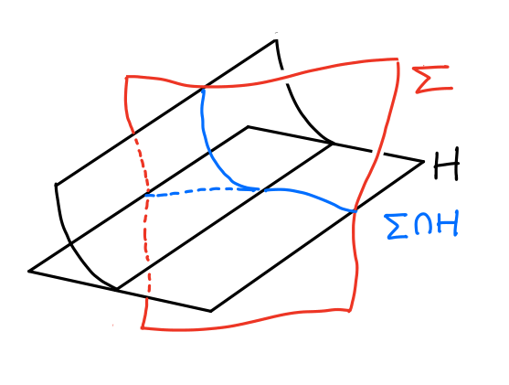
Let H⊂MH\subset M be an arboreal front. Then for any submanifold Σ⊂M\Sigma\subset M transverse to (all strata of) HH the intersection Σ∩H\Sigma\cap H is an arboreal front in Σ\Sigma.

Proof.

We can assume that HH is an arboreal front germ at a point x∈Hx\in H, and hence the germ of (M,H)(M,H) at xx is diffeomorphic to the germ of (ℝn⁡(𝒯^)+1×ℝk,H𝒯^×ℝk)({\mathbb{R}}^{n({\widehat{\mathscr{T}}})+1}\times{\mathbb{R}}^{k},H_{\widehat{\mathscr{T}}}\times{\mathbb{R}}^{k}) for some rooted signed arboreal tree 𝒯^{\widehat{\mathscr{T}}} and k=n−n⁡(𝒯^)k=n-n({\widehat{\mathscr{T}}}). Note that the transversality of Σ\Sigma to HH implies that codim​Σ≤k{\rm codim}\Sigma\leq k and that the projection of p:Σ⊂ℝn⁡(𝒯^)+1×ℝk→ℝn⁡(𝒯^)+1p:\Sigma\subset{\mathbb{R}}^{n({\widehat{\mathscr{T}}})+1}\times{\mathbb{R}}^{k}\to{\mathbb{R}}^{n({\widehat{\mathscr{T}}})+1} to the first factor is a submersion, and because we are dealing with germs, it is a trivial fibration. On the other hand, the projection p|Σ∩H:Σ∩H→H𝒯^p|_{\Sigma\cap H}:\Sigma\cap H\to H_{\widehat{\mathscr{T}}} is the restriction of this fibration to H𝒯^⊂ℝN⁡(𝒯^)H_{\widehat{\mathscr{T}}}\subset{\mathbb{R}}^{N({\widehat{\mathscr{T}}})}. ∎

Refer to caption
Figure 3.3. Illustration that Σ∩H\Sigma\cap H is an arboreal front in Σ\Sigma.

3.3. Parametric version

The following is the parametric version of Theorem 3.5.

Theorem 3.12.

Let 𝒯^{\widehat{\mathscr{T}}} be a signed rooted tree. Let ρ1,…,ρk\rho_{1},\dots,\rho_{k} be vertices adjacent to the root ρ\rho and 𝒯^j{\widehat{\mathscr{T}}}_{j} be subtrees with roots ρj\rho_{j} (where we removed the decoration of edges [ρj​α][\rho_{j}\alpha]). Let ϕjy:t∗​ℝm→J1​ℝm\phi^{y}_{j}:\mathrm{t}^{*}{\mathbb{R}}^{m}\to J^{1}{\mathbb{R}}^{m}, m≥n=n⁡(𝒯)m\geq n=n(\mathscr{T}), be families of germs of Weinstein hypersurface embeddings with disjoint images, parametrized by a manifold YY. Denote zjy:=ϕjy​(0)z^{y}_{j}:=\phi^{y}_{j}(0), Λyj=ϕjy​(L𝒯^j×ℝm−n⁡(𝒯^j))\Lambda_{y}^{j}=\phi^{y}_{j}(L_{{\widehat{\mathscr{T}}}_{j}}\times{\mathbb{R}}^{m-n({\widehat{\mathscr{T}}}_{j})}), j=1,…,kj=1,\dots,k. Suppose that

  • (i)

    π⁡(zjy)=0\pi(z^{y}_{j})=0;

  • (ii)

    the arboreal Legendrian Λy:=⋃j=1kΛyj\Lambda_{y}:=\bigcup_{j=1}^{k}\Lambda_{y}^{j} projects transversely under the front projection J1​ℝn→ℝ×ℝnJ^{1}{\mathbb{R}}^{n}\to{\mathbb{R}}\times{\mathbb{R}}^{n};

  • (iii)

    for each edge [ρj​α][\rho_{j}\alpha] we have ε⁡(ν,Λyj,α)=ε[ρj​α]\varepsilon(\nu,\Lambda^{j}_{y},\alpha)=\varepsilon_{[\rho_{j}\alpha]}.

Then there exists a family of diffeomorphisms ϕy\phi_{y} between H𝒯^×ℝm−n⁡(𝒯^)H_{\widehat{\mathscr{T}}}\times{\mathbb{R}}^{m-n({\widehat{\mathscr{T}}})} and the front π⁡(Λy)\pi(\Lambda_{y}). If K⊂YK\subset Y is a closed subset and the ϕjy\phi_{j}^{y} are the standard embeddings of the local model for y∈𝒪​p​(K)y\in{\mathcal{O}}{\it p}\,(K), then we may further assume ϕy=Id\phi_{y}=\text{Id} for y∈𝒪​p​(K)y\in{\mathcal{O}}{\it p}\,(K).

The parametric version of Proposition 3.6 is formulated similarly. As a consequence of Theorem 3.12 we get the following result:

Corollary 3.13.

Fix a signed rooted tree 𝒯^=(T,ρ,ε){\widehat{\mathscr{T}}}=(T,\rho,\varepsilon), set n=|n⁡(𝒯^)|n=|n({\widehat{\mathscr{T}}})| and consider the arboreal 𝒯^{\widehat{\mathscr{T}}}-front H𝒯^⊂ℝnH_{\widehat{\mathscr{T}}}\subset{\mathbb{R}}^{n}. Let D⁡(ℝn,H𝒯^)D({\mathbb{R}}^{n},H_{\widehat{\mathscr{T}}}) be the group of germs at 00 of diffeomorphisms of ℝn{\mathbb{R}}^{n} preserving H𝒯^H_{\widehat{\mathscr{T}}} as a front, i.e.  as a subset along with its coorientation.

Then the fibers of the natural map D⁡(ℝn,H𝒯^)→Aut⁡(𝒯^)D({\mathbb{R}}^{n},H_{\widehat{\mathscr{T}}})\to{\rm Aut}({\widehat{\mathscr{T}}}) are weakly contractible.

Proof.

We deduce Corollary  3.13 from Theorem 3.12. We will argue for 𝒯^=𝒜n+1{\widehat{\mathscr{T}}}=\mathcal{A}_{n+1} when H𝒜n+1=Γn−1H_{\mathcal{A}_{n+1}}={}^{n-1}\Gamma; the case of general 𝒯^{\widehat{\mathscr{T}}} is similar.

Since Aut⁡(𝒜n+1){\rm Aut}(\mathcal{A}_{n+1}) is trivial, we seek to show D⁡(ℝn,Γn−1)D({\mathbb{R}}^{n},{}^{n-1}\Gamma) is weakly contractible. Note any φ∈D⁡(ℝn,Γn−1)\varphi\in D({\mathbb{R}}^{n},{}^{n-1}\Gamma) preserves 00, and moreover, preserves the canonical flag in T0​ℝnT_{0}{\mathbb{R}}^{n} given by the tangents to the intersections ⋂i<i0Γin−1\bigcap_{i<i_{0}}{}^{n-1}\Gamma_{i}.

Let D⁡(ℝn)D({\mathbb{R}}^{n}) denote the group of germs at 00 of diffeomorphisms of ℝn{\mathbb{R}}^{n}. Consider a kk-sphere of maps ft∈D⁡(ℝn,Γn−1)f_{t}\in D({\mathbb{R}}^{n},{}^{n-1}\Gamma), t∈Skt\in S^{k}. Since all ftf_{t} preserve 00 and the canonical flag in T0​ℝnT_{0}{\mathbb{R}}^{n}, there exists a k+1k+1-ball of diffeomorphisms gt∈D⁡(ℝn)g_{t}\in D({\mathbb{R}}^{n}), t∈Bk+1t\in B^{k+1}, extending ftf_{t}. Applying Theorem 3.12 to the Weinstein hypersurface embeddings induced by gtg_{t}, we can find diffeomorphisms hth_{t} such that hth_{t} takes gt​(Γn−1)g_{t}({}^{n-1}\Gamma) back to Γn−1{}^{n-1}\Gamma and such that hth_{t} is the identity for t∈Skt\in S^{k}. Then ht∘gt∈D⁡(ℝn,Γn−1)h_{t}\circ g_{t}\in D({\mathbb{R}}^{n},{}^{n-1}\Gamma), t∈Bk+1t\in B^{k+1}, gives an extension of ftf_{t} to the k+1k+1-ball. ∎

We also formulate the parametric version of Corollary 3.10.

Corollary 3.14.

Let L𝒯^⊂T∗​ℝnL_{\widehat{\mathscr{T}}}\subset T^{*}{\mathbb{R}}^{n} be a model Lagrangian associated with a signed rooted tree (T,ρ,ε)(T,\rho,\varepsilon). Let η0y,η1y\eta^{y}_{0},\eta^{y}_{1} be two families of polarizations transverse to L𝒯^L_{\widehat{\mathscr{T}}} parametrized by a manifold YY. Suppose that for any vertex α\alpha of TT adjacent to ρ\rho we have

ε⁡(η0y,L,α)=ε⁡(η1y,L,α).\varepsilon(\eta^{y}_{0},L,\alpha)=\varepsilon(\eta^{y}_{1},L,\alpha).

Then there is a family of (germ at the origin of) symplectomorphisms ψy:T∗​ℝn→T∗​ℝn\psi^{y}:T^{*}{\mathbb{R}}^{n}\to T^{*}{\mathbb{R}}^{n} such that ψy​(L)=L\psi^{y}(L)=L and d​ψy​(η0y)=η1yd\psi^{y}(\eta^{y}_{0})=\eta^{y}_{1} along LL. Moreover, if η0y=η1y\eta_{0}^{y}=\eta_{1}^{y} for y∈𝒪​p​(K)y\in{\mathcal{O}}{\it p}\,(K) for K⊂YK\subset Y a closed subset, then we can take ψy=Id\psi^{y}=\text{Id} for y∈𝒪​p​(K)y\in{\mathcal{O}}{\it p}\,(K).

The proof is just like in the non-parametric case, but applying Theorem 3.12 instead of Theorem 3.5.

3.4. Tangency loci

Before proving Proposition 3.6 and its parametric analogue we need to analyze more closely the geometry of hypersurfaces forming arboreal fronts.

Definition 3.15.

Given smooth hypersurfaces X1,X2⊂ℝn+1X_{1},X_{2}\subset{\mathbb{R}}^{n+1}, we denote by T⁡(X1,X2)⊂ℝn+1T(X_{1},X_{2})\subset{\mathbb{R}}^{n+1} their tangency locus, i.e. the subset of points x∈X1∩X2x\in X_{1}\cap X_{2} such that Tx​X1=Tx​X2T_{x}X_{1}=T_{x}X_{2}.

Remark 3.16.

Given smooth Legendrians L1,L2⊂J1​ℝnL_{1},L_{2}\subset J^{1}{\mathbb{R}}^{n} whose fronts X1=π⁡(L1),X2=π⁡(L2)⊂ℝn+1X_{1}=\pi(L_{1}),X_{2}=\pi(L_{2})\subset{\mathbb{R}}^{n+1} are smooth hypersurfaces, note that T⁡(X1,X2)=π⁡(L1∩L2)T(X_{1},X_{2})=\pi(L_{1}\cap L_{2}).

For 0≤j<i≤n0\leq j<i\leq n, recall the notation

hi,j:=hi−j​(xj+1,…,xi)\textstyle{h_{i,j}:=h_{i-j}(x_{j+1},\ldots,x_{i})}

so in particular hi,0=hi​(x1,…,xi)h_{i,0}=h_{i}(x_{1},\ldots,x_{i}) and hi,i−1=h1​(xi)=xih_{i,i-1}=h_{1}(x_{i})=x_{i}. Set

Ti,j={hi,j=0}⊂ℝn+1\textstyle{T_{i,j}=\{h_{i,j}=0\}\subset{\mathbb{R}}^{n+1}}

Note hi,jh_{i,j} is independent of x0,…,xjx_{0},\ldots,x_{j}, and we have

Ti,j=ℝj+1×Γi−j−1n−j−1T_{i,j}={\mathbb{R}}^{j+1}\times{}^{n-j-1}\Gamma_{i-j-1}
Lemma 3.17.

For 0≤j<i≤n0\leq j<i\leq n, the tangency locus T⁡(Γin,Γjn)⊂ℝn+1T({}^{n}\Gamma_{i},{}^{n}\Gamma_{j})\subset{\mathbb{R}}^{n+1} is the intersection of either Γin{}^{n}\Gamma_{i} or Γjn{}^{n}\Gamma_{j} with the union

{hi,j=0}∪⋃k=0j−1{hi,k=hj,k=0}=Ti,j∪⋃k=0j−1(Ti,k∩Tj,k)\textstyle{\{h_{i,j}=0\}\cup\bigcup\limits_{k=0}^{j-1}\{h_{i,k}=h_{j,k}=0\}=T_{i,j}\cup\bigcup\limits_{k=0}^{j-1}(T_{i,k}\cap T_{j,k})}
Proof.

Since Γin,Γjn{}^{n}\Gamma_{i},{}^{n}\Gamma_{j} are the graphs of hi2,hj2h_{i}^{2},h_{j}^{2}, the projection of T⁡(ΓinCLOSET({}^{n}\Gamma_{i}, OPENΓjn){}^{n}\Gamma_{j}) to the domain ℝn{\mathbb{R}}^{n} is cut out by

hi2=hj2\textstyle{h_{i}^{2}=h_{j}^{2}}d​hi2=d​hj2\textstyle{dh^{2}_{i}=dh^{2}_{j}}

Note hi=hi,0=x1−hi,12h_{i}=h_{i,0}=x_{1}-h_{i,1}^{2}, hj=hj,0=x1−hj,12h_{j}=h_{j,0}=x_{1}-h_{j,1}^{2}. By examining the d​x1dx_{1}-component of d​hi2=d​hj2dh^{2}_{i}=dh^{2}_{j}, we see it implies hi=hjh_{i}=h_{j}. Thus the projection of T⁡(ΓinCLOSET({}^{n}\Gamma_{i}, OPENΓjn){}^{n}\Gamma_{j}) is cut out by the single equation d​hi2=d​hj2dh^{2}_{i}=dh^{2}_{j} which in turn implies hi=hjh_{i}=h_{j}.

To satisfy d​hi2=d​hj2dh^{2}_{i}=dh^{2}_{j}, so in particular hi=hjh_{i}=h_{j}, there are two possibilities: (i) hi=hj=0h_{i}=h_{j}=0; or (ii) hi=hj≠0h_{i}=h_{j}\not=0. In case (i), we find the subset {hi,0=hj,0=0}\{h_{i,0}=h_{j,0}=0\} appearing in the union of the assertion of the lemma. In case (ii), we observe d​hi2=d​hj2dh^{2}_{i}=dh^{2}_{j} is then equivalent to d​hi,12=d​hj,12dh^{2}_{i,1}=dh^{2}_{j,1} which in turn implies hi,1=hj,1h_{i,1}=h_{j,1}.

Now we repeat the argument. To satisfy d​hi,12=d​hj,12,dh^{2}_{i,1}=dh^{2}_{j,1}, so in particular hi,1=hj,1h_{i,1}=h_{j,1}, there are two possibilities: (i) hi,1=hj,1=0h_{i,1}=h_{j,1}=0; or (ii) hi,1=hj,1≠0h_{i,1}=h_{j,1}\not=0. In case (i), we find the subset {hi,1=hj,1=0}\{h_{i,1}=h_{j,1}=0\} appearing in the union of the assertion of the lemma. In case (ii), we observe d​hi,12=d​hj,12dh^{2}_{i,1}=dh^{2}_{j,1} is then equivalent to d​hi,22=d​hj,22dh^{2}_{i,2}=dh^{2}_{j,2} which in turn implies hi,2=hj,2h_{i,2}=h_{j,2}.

Iterating this argument, we obtain the subset ⋃k=0j−1{hi,k=hj,k=0}\bigcup_{k=0}^{j-1}\{h_{i,k}=h_{j,k}=0\}, and arrive at the final equation d​hi,j2=0.dh^{2}_{i,j}=0. By examining the d​xj+1dx_{j+1}-term, we see d​hi,j2=0dh^{2}_{i,j}=0 holds if and only if hi,j=0h_{i,j}=0, which gives the remaining subset of the assertion of the lemma. ∎

Remark 3.18.

The only evident redundancy in the description of the lemma is Ti,j−1∩Tj,j−1⊂Ti,jT_{i,j-1}\cap T_{j,j-1}\subset T_{i,j} since hi,j−1=xj−hi,j2h_{i,j-1}=x_{j}-h_{i,j}^{2}, hj,j−1=xjh_{j,j-1}=x_{j}, so their vanishing implies the vanishing of hi,jh_{i,j}.

We will be particularly interested in the locus Ti,j⊂T⁡(Γin,Γjn)T_{i,j}\subset T({}^{n}\Gamma_{i},{}^{n}\Gamma_{j}) and formalize its structure in the following definition.

Definition 3.19.

Given smooth hypersurfaces X1,X2⊂ℝn+1X_{1},X_{2}\subset{\mathbb{R}}^{n+1}, we denote by τ∘​(X1,X2)⊂T⁡(X1,X2)\tau^{\circ}(X_{1},X_{2})\subset T(X_{1},X_{2}) the subset of points x∈X1∩X2x\in X_{1}\cap X_{2} where in some local coordinates we have X1={x0=0}X_{1}=\{x_{0}=0\}, X2={x0=x12}X_{2}=\{x_{0}=x_{1}^{2}\}. We write τ⁡(X1,X2)⊂T⁡(X1,X2)\tau(X_{1},X_{2})\subset T(X_{1},X_{2}) for the closure of τ∘​(X1,X2)\tau^{\circ}(X_{1},X_{2}), and refer to it as the primary tangency of X1,X2X_{1},X_{2}.

Remark 3.20.

Given smooth Legendrians L1,L2⊂J1​ℝnL_{1},L_{2}\subset J^{1}{\mathbb{R}}^{n} whose fronts X1=π⁡(L1),X2=π⁡(L2)⊂ℝn+1X_{1}=\pi(L_{1}),X_{2}=\pi(L_{2})\subset{\mathbb{R}}^{n+1} are smooth hypersurfaces, note that τ∘​(X1,X2)\tau^{\circ}(X_{1},X_{2}) is the front projection of where L1,L2L_{1},L_{2} intersect cleanly in codimension one.

We have the following consequence of Lemma 3.17.

Corollary 3.21.

For 0≤j<i≤n0\leq j<i\leq n, the primary tangency τ⁡(Γin,Γjn)⊂ℝn+1\tau({}^{n}\Gamma_{i},{}^{n}\Gamma_{j})\subset{\mathbb{R}}^{n+1} is the intersection of either Γin{}^{n}\Gamma_{i} or Γjn{}^{n}\Gamma_{j} with Ti,jT_{i,j}.

Before continuing, let us record the following for future use.

Lemma 3.22.

Fix 0≤k<j≤n−10\leq k<j\leq n-1.

We have

τ⁡(τ⁡(Γn,Γkn),τ⁡(Γjn,Γkn))=τ⁡(Γnn,Γjn)∩τ⁡(Γjn,Γkn)\textstyle{\tau(\tau(\Gamma_{n},{}^{n}\Gamma_{k}),\tau({}^{n}\Gamma_{j},{}^{n}\Gamma_{k}))=\tau({}^{n}\Gamma_{n},{}^{n}\Gamma_{j})\cap\tau({}^{n}\Gamma_{j},{}^{n}\Gamma_{k})}

where the primary tangency of τ⁡(Γn,Γkn)\tau(\Gamma_{n},{}^{n}\Gamma_{k}), τ⁡(Γjn,Γkn)\tau({}^{n}\Gamma_{j},{}^{n}\Gamma_{k}) of the left hand side is calculated in Γkn≃ℝn{}^{n}\Gamma_{k}\simeq{\mathbb{R}}^{n}.

Figure 3.4. Verification of the conclusion of Lemma 3.22 for n=2n=2, in this case both the right and left hand sides of the equality τ⁡(τ⁡(Γ22,Γ02),τ⁡(Γ12,Γ02))=τ⁡(Γ22,Γ12)∩τ⁡(Γ12,Γ02)\tau(\tau({}^{2}\Gamma_{2},{}^{2}\Gamma_{0}),\tau({}^{2}\Gamma_{1},{}^{2}\Gamma_{0}))=\tau({}^{2}\Gamma_{2},{}^{2}\Gamma_{1})\cap\tau({}^{2}\Gamma_{1},{}^{2}\Gamma_{0}) consist of the origin.
Proof.

By the preceding corollary, the left hand side is the intersection Γkn∩τ⁡(Tn,k,Tj,k){}^{n}\Gamma_{k}\cap\tau(T_{n,k},T_{j,k}).

Note Γkn∩Tj,k=τ⁡(Γjn,Γkn)=Γjn∩Tj,k{}^{n}\Gamma_{k}\cap T_{j,k}=\tau({}^{n}\Gamma_{j},{}^{n}\Gamma_{k})={}^{n}\Gamma_{j}\cap T_{j,k}. Hence

Γkn∩τ⁡(Tn,k,Tj,k)=Γjn∩τ⁡(Tn,k,Tj,k){}^{n}\Gamma_{k}\cap\tau(T_{n,k},T_{j,k})={}^{n}\Gamma_{j}\cap\tau(T_{n,k},T_{j,k})

since y∈Γkn∩τ⁡(Tn,k,Tj,k)y\in{}^{n}\Gamma_{k}\cap\tau(T_{n,k},T_{j,k}) ⇔\iff y∈Γkn∩Tj,ky\in{}^{n}\Gamma_{k}\cap T_{j,k}, y∈τ⁡(Tn,k,Tj,k)y\in\tau(T_{n,k},T_{j,k}) ⇔\iff y∈Γjn∩Tj,ky\in{}^{n}\Gamma_{j}\cap T_{j,k}, y∈τ⁡(Tn,k,Tj,k)y\in\tau(T_{n,k},T_{j,k}) ⇔\iff y∈Γjn∩τ⁡(Tn,k,Tj,k)y\in{}^{n}\Gamma_{j}\cap\tau(T_{n,k},T_{j,k}).

Next, recall

Tn,k=ℝk+1×Γn−k−1n−k−1\textstyle{T_{n,k}={\mathbb{R}}^{k+1}\times{}^{n-k-1}\Gamma_{n-k-1}}Tj,k=ℝk+1×Γj−k−1n−k−1\textstyle{T_{j,k}={\mathbb{R}}^{k+1}\times{}^{n-k-1}\Gamma_{j-k-1}}

Hence by the preceding corollary, we have

τ(Tn,k,Tj,k)=Tj,k∩{hn,j=0}\textstyle{\tau(T_{n,k},T_{j,k})=T_{j,k}\cap\{h_{n,j}=0\}}

Thus the left hand side is given by Γjn∩Tj,k∩Tn,j{}^{n}\Gamma_{j}\cap T_{j,k}\cap T_{n,j}.

On the other hand, by the preceding corollary, the right hand side is also given by Γjn∩Tn,j∩Tj,k.{}^{n}\Gamma_{j}\cap T_{n,j}\cap T_{j,k}. ∎

3.4.1. More on distinguished quadrants

Corollary 3.23.

For 0≤j<i≤n0\leq j<i\leq n, we have

Γiεn∩Γjεn=T⁡(Γiεn,Γjεn)=τ⁡(Γiεn,Γjεn)\textstyle{{}^{n}\Gamma^{\varepsilon}_{i}\cap{}^{n}\Gamma^{\varepsilon}_{j}=T({}^{n}\Gamma^{\varepsilon}_{i},{}^{n}\Gamma^{\varepsilon}_{j})=\tau({}^{n}\Gamma^{\varepsilon}_{i},{}^{n}\Gamma^{\varepsilon}_{j})}

and they coincide with the closed boundary face of Γiεn{}^{n}\Gamma^{\varepsilon}_{i} cut out by hi,j=0.h_{i,j}=0.

Proof.

For j=0j=0, we have Γ0εn=Γ0n={x0=0}{}^{n}\Gamma^{\varepsilon}_{0}={}^{n}\Gamma_{0}=\{x_{0}=0\}. From the definitions, we have

Γiεn∩Γ0n=T⁡(Γiεn,Γ0n)=τ⁡(Γiεn,Γ0n)\textstyle{{}^{n}\Gamma^{\varepsilon}_{i}\cap{}^{n}\Gamma_{0}=T({}^{n}\Gamma^{\varepsilon}_{i},{}^{n}\Gamma_{0})=\tau({}^{n}\Gamma^{\varepsilon}_{i},{}^{n}\Gamma_{0})}

which is cut out of Piεn{}^{n}P^{\varepsilon}_{i} by hi,0=hi=0.h_{i,0}=h_{i}=0.

For j>0j>0, the assertions follow from Lemma 2.4 by induction on nn. ∎

Remark 3.24.

Note for any 0≤j<i≤n0\leq j<i\leq n, we have

τ⁡(Γin,Γjn)=⋃ετ⁡(Γiεn,Γjεn)\textstyle{\tau({}^{n}\Gamma_{i},{}^{n}\Gamma_{j})=\bigcup_{\varepsilon}\tau({}^{n}\Gamma^{\varepsilon}_{i},{}^{n}\Gamma^{\varepsilon}_{j})}

To see this, consider x∈τ⁡(Γin,Γjn)x\in\tau({}^{n}\Gamma_{i},{}^{n}\Gamma_{j}), so that hi,j​(x)=0h_{i,j}(x)=0 by Corollary 3.21. Choose ε\varepsilon so that x∈Γiεnx\in{}^{n}\Gamma^{\varepsilon}_{i}. Then by Corollary 3.23, we have x∈τ⁡(Γiεn,Γjεn)x\in\tau({}^{n}\Gamma^{\varepsilon}_{i},{}^{n}\Gamma^{\varepsilon}_{j}).

For i=0i=0, let L0εn=ℝn⊂T∗​ℝn{}^{n}L^{\varepsilon}_{0}={\mathbb{R}}^{n}\subset T^{*}{\mathbb{R}}^{n} denote the zero-section. For i=1,…,ni=1,\ldots,n, consider the conormal bundles

Liεn=TΓi−1εn−1∗​ℝn⊂T∗​ℝn\textstyle{{}^{n}L^{\varepsilon}_{i}=T^{*}_{{}^{n-1}\Gamma^{\varepsilon}_{i-1}}{\mathbb{R}}^{n}\subset T^{*}{\mathbb{R}}^{n}}

and their union

Lεn=⋃i=0nLiεn\textstyle{{}^{n}L^{\varepsilon}=\bigcup_{i=0}^{n}{}^{n}L^{\varepsilon}_{i}}

Similarly, for i=0,…,ni=0,\ldots,n, consider the smooth Legendrian

Λiεn⊂J1​ℝn\textstyle{{}^{n}\Lambda^{\varepsilon}_{i}\subset J^{1}{\mathbb{R}}^{n}}

that maps diffeomorphically to Γiεn⊂ℝn+1{}^{n}\Gamma^{\varepsilon}_{i}\subset{\mathbb{R}}^{n+1} under the front projection π:J1​ℝn→ℝn+1\pi:J^{1}{\mathbb{R}}^{n}\to{\mathbb{R}}^{n+1}, and their union

Λεn=⋃i=0nΛiεn\textstyle{{}^{n}\Lambda^{\varepsilon}=\bigcup_{i=0}^{n}{}^{n}\Lambda^{\varepsilon}_{i}}

Note the contactomorphism of Lemma 2.1 takes Λiεn⊂J1​ℝn{}^{n}\Lambda^{\varepsilon}_{i}\subset J^{1}{\mathbb{R}}^{n} isomorphically to {0}×Liεn⊂{0}×T∗​ℝn\{0\}\times{}^{n}L^{\varepsilon}_{i}\subset\{0\}\times T^{*}{\mathbb{R}}^{n}, and thus Λεn⊂J1​ℝn{}^{n}\Lambda^{\varepsilon}\subset J^{1}{\mathbb{R}}^{n} isomorphically to {0}×Lεn⊂{0}×T∗​ℝn\{0\}\times{}^{n}L^{\varepsilon}\subset\{0\}\times T^{*}{\mathbb{R}}^{n}.

We have the following topological consequence of Lemma 2.4.

Corollary 3.25.

As a union of smooth manifolds with corners, Γεn⊂ℝn+1{}^{n}\Gamma^{\varepsilon}\subset{\mathbb{R}}^{n+1} is given by the gluing

Γεn=(Γε′n−1×ℝ≥0)​∐(Γε′n−1×{0})(ℝn×{0})\textstyle{{}^{n}\Gamma^{\varepsilon}=({}^{n-1}\Gamma^{\varepsilon^{\prime}}\times{\mathbb{R}}_{\geq 0})\coprod_{({}^{n-1}\Gamma^{\varepsilon^{\prime}}\times\{0\})}({\mathbb{R}}^{n}\times\{0\})}

where ε′=(ε0​ε1,ε2,…,εn)\varepsilon^{\prime}=(\varepsilon_{0}\varepsilon_{1},\varepsilon_{2},\ldots,\varepsilon_{n}). The front projection takes Lεn⊂J1​ℝn{}^{n}L^{\varepsilon}\subset J^{1}{\mathbb{R}}^{n} homeomorphically to Γεn⊂ℝn+1{}^{n}\Gamma^{\varepsilon}\subset{\mathbb{R}}^{n+1}.

Before continuing, let us record the following for future use.

Corollary 3.26.

For 0<j<i≤n0<j<i\leq n, the closure of the codimension one clean intersection of Liεn,Ljn{}^{n}L^{\varepsilon}_{i},{}^{n}L_{j} is precisely Liεn∩Ljεn{}^{n}L^{\varepsilon}_{i}\cap{}^{n}L^{\varepsilon}_{j}.

Proof.

The closure of the codimension one clean intersection of Liεn,Λjn{}^{n}L^{\varepsilon}_{i},{}^{n}\Lambda_{j} is conic and projects to the primary tangency of Γi−1εn−1,Γj−1n−1{}^{n-1}\Gamma^{\varepsilon}_{i-1},{}^{n-1}\Gamma_{j-1}. By Corollary 3.21, the primary tangency of Γi−1n−1,Γj−1n−1{}^{n-1}\Gamma_{i-1},{}^{n-1}\Gamma_{j-1} is cut out by hi−1,j−1=0h_{i-1,j-1}=0. By Corollary 3.23, this is precisely the tangency T⁡(Γi−1εn−1,Γj−1n−1)T({}^{n-1}\Gamma^{\varepsilon}_{i-1},{}^{n-1}\Gamma_{j-1}) and hence lifts precisely to the conic intersection Liεn∩Ljεn{}^{n}L^{\varepsilon}_{i}\cap{}^{n}L^{\varepsilon}_{j}. ∎

3.5. The case of 𝒜n+1\mathscr{A}_{n+1}-tree

The following Theorem 3.27 will play a key role in proving Proposition 3.6.

Theorem 3.27.

Let φ:T∗​ℝn→J1​ℝn\varphi:T^{*}{\mathbb{R}}^{n}\to J^{1}{\mathbb{R}}^{n} be an embedding as a Weinstein hypersurface. Assume that the image of Ln{}^{n}L under φ\varphi is transverse to the fibers of the projection J1​ℝn→ℝnJ^{1}{\mathbb{R}}^{n}\to{\mathbb{R}}^{n}. Let Υ=π⁡(φ⁡(Ln))⊂ℝ×ℝn\Upsilon=\pi(\varphi({}^{n}L))\subset{\mathbb{R}}\times{\mathbb{R}}^{n} be (the germ of) the front at the central point.

Then there exists a diffeomorphism ℝ×ℝn→ℝ×ℝn{\mathbb{R}}\times{\mathbb{R}}^{n}\to{\mathbb{R}}\times{\mathbb{R}}^{n} taking Υ\Upsilon to the germ at the origin of Γn⊂ℝ×ℝn{}^{n}\Gamma\subset{\mathbb{R}}\times{\mathbb{R}}^{n}.

The proof of Theorem 3.27 will proceed by induction on the dimension nn. At each stage, we will prove the fully parametric version:

Theorem 3.28.

Let φy:T∗​ℝn→J1​ℝn\varphi^{y}:T^{*}{\mathbb{R}}^{n}\to J^{1}{\mathbb{R}}^{n} be a family of Weinstein hypersurface embeddings parametrized by a manifold YY. Assume that the image of Ln{}^{n}L under φy\varphi^{y} is transverse to the fibers of the projection J1​ℝn→ℝnJ^{1}{\mathbb{R}}^{n}\to{\mathbb{R}}^{n}. Let Υy=π⁡(φy​(Ln))⊂ℝ×ℝn\Upsilon^{y}=\pi(\varphi^{y}({}^{n}L))\subset{\mathbb{R}}\times{\mathbb{R}}^{n} be (the germs of) the fronts at the central points.

Then there exists a family of diffeomorphisms ψy:ℝ×ℝn→ℝ×ℝn\psi^{y}:{\mathbb{R}}\times{\mathbb{R}}^{n}\to{\mathbb{R}}\times{\mathbb{R}}^{n} taking Υy\Upsilon^{y} to the germ at the origin of Γn⊂ℝ×ℝn{}^{n}\Gamma\subset{\mathbb{R}}\times{\mathbb{R}}^{n}. If φy=Id\varphi^{y}=\text{Id} for y∈𝒪​p​(K)y\in{\mathcal{O}}{\it p}\,(K), where K⊂YK\subset Y is a closed subset, then we may assume ψy=Id\psi^{y}=\text{Id} for y∈𝒪​p​(K)y\in{\mathcal{O}}{\it p}\,(K).

As usual the case of general pairs (Y,K)(Y,K) follows from the case Y=DkY=D^{k} and K=Sk−1K=S^{k-1}.

3.5.1. Base case n=0n=0

The kk-parametric version states: the germ of any graphical hypersurface Υ⊂ℝ×ℝk\Upsilon\subset{\mathbb{R}}\times{\mathbb{R}}^{k} is diffeomorphic to the germ of the zero-graph Γ0×ℝk={0}×ℝk{}^{0}\Gamma\times{\mathbb{R}}^{k}=\{0\}\times{\mathbb{R}}^{k}. This can be achieved by an isotopy generated by a time-dependent vector field of the form ht∂x0h_{t}\partial_{x_{0}}. This vector field is zero at infinity if Υ\Upsilon is standard at infinity.

3.5.2. Case n=1n=1

The next case of the induction n=1n=1 is elementary but slightly different from the others, so it is more convenient to treat separately.

With the setup of the theorem, consider the front Υ=π⁡(Λ1)⊂ℝ2\Upsilon=\pi({}^{1}\Lambda)\subset{\mathbb{R}}^{2}, and assume without loss of generality that the origin is the central point. By induction, we may assume, the front takes the form Υ=Γ0∪Υ1⊂ℝ2\Upsilon=\Gamma_{0}\cup\Upsilon_{1}\subset{\mathbb{R}}^{2} where Γ0={x0=0}\Gamma_{0}=\{x_{0}=0\}. Near the origin, the intersection Γ0∩Υ1\Gamma_{0}\cap\Upsilon_{1} and tangency locus T⁡(Γ0,Υ1)T(\Gamma_{0},\Upsilon_{1}) coincide and consist of the origin alone. Moreover, by construction, the origin is a simple tangency, and so Υ1={x0=αx12}\Upsilon_{1}=\{x_{0}=\alpha x_{1}^{2}\} with α⁡(0)≠0\alpha(0)\not=0. Now it is elementary to find a time-dependent vector field of the form htx1∂x1h_{t}x_{1}\partial_{x_{1}}, hence vanishing on Γ0\Gamma_{0}, generating an isotopy taking Υ1\Upsilon_{1} to either Γ1={x0=x12}\Gamma_{1}=\{x_{0}=x_{1}^{2}\} or −Γ1={x0=−x12}-\Gamma_{1}=\{x_{0}=-x_{1}^{2}\}. In the former case, we are done; in the latter case, we may apply the diffeomorphism (x0,x1)↦(−x0,x1)(x_{0},x_{1})\mapsto(-x_{0},x_{1}) to arrive at the configuration Γ0∪Γ1\Gamma_{0}\cup\Gamma_{1}. Finally, it is evident the prior constructions can be performed parametrically, with the vector field zero at infinity if Υ\Upsilon is standard at infinity.

3.5.3. Inductive step

The inductive step takes the following form. Suppose the fully parametric assertion has been established for dimension n−1n-1. Starting from Λn⊂T∗​ℝn{}^{n}\Lambda\subset T^{*}{\mathbb{R}}^{n}, remove the last smooth piece to obtain Λ′n=Λn∖Λnn{}^{n}\Lambda^{\prime}={}^{n}\Lambda\setminus{}^{n}\Lambda_{n}, and consider the corresponding front Υ′=π⁡(Λ′n)\Upsilon^{\prime}=\pi({}^{n}\Lambda^{\prime}). Note that Λ′n=Λn−1×ℝ⊂T∗​(ℝn−1×ℝ){}^{n}\Lambda^{\prime}={}^{n-1}\Lambda\times{\mathbb{R}}\subset T^{*}({\mathbb{R}}^{n-1}\times{\mathbb{R}}), and so by an inductive application of the 1-parametric version of the theorem, we may assume

Υ′=Γn−1×ℝ\textstyle{\Upsilon^{\prime}={}^{n-1}\Gamma\times{\mathbb{R}}}

Set Υn=π⁡(Λnn)\Upsilon_{n}=\pi({}^{n}\Lambda_{n}). We will find a diffeomorphism ℝn+1→ℝn+1{\mathbb{R}}^{n+1}\to{\mathbb{R}}^{n+1} that preserves Υ′\Upsilon^{\prime} (as a subset, not pointwise), and takes Υn\Upsilon_{n} to Γnn{}^{n}\Gamma_{n}. Moreover, it will be evident the diffeomorphism can be constructed in parametric form, including the relative parametric form. This will complete the inductive step and prove the theorem.

3.5.4. Two propositions

The proof of the inductive step is based on the following 2 propositions.

Proposition 3.29.

Fix n≥2n\geq 2.

With the setup of Theorem 3.27, suppose Υ=⋃i=0n−1Γin∪Υn\Upsilon=\bigcup_{i=0}^{n-1}{}^{n}\Gamma_{i}\cup\Upsilon_{n} where Υn=π⁡(Λnn)\Upsilon_{n}=\pi({}^{n}\Lambda_{n}). Suppose in addition Υn\Upsilon_{n} has primary tangency loci satisfying

τ⁡(Υn,Γin)⊃τ⁡(Γnn,Γin)\textstyle{\tau(\Upsilon_{n},{}^{n}\Gamma_{i})\supset\tau({}^{n}\Gamma_{n},{}^{n}\Gamma_{i})}i=0,…,n−1\textstyle{i=0,\ldots,n-1}

Then Υn={x0=αhn2}\Upsilon_{n}=\{x_{0}=\alpha h^{2}_{n}\} where

α=1+β∏j=1n−1h2n,j=1+βh2n,1⋯h2n,n−1\textstyle{\alpha=1+\beta\prod\limits_{j=1}^{n-1}h^{2}_{n,j}=1+\beta h^{2}_{n,1}\cdots h^{2}_{n,n-1}}

Moreover, the same holds in parametric form.

Proof.

We have Υn={x0=g}\Upsilon_{n}=\{x_{0}=g\} for some gg. Since τ(Υn,Γ0n)⊃τ(Γnn,Γ0n)={hn=0}\tau(\Upsilon_{n},{}^{n}\Gamma_{0})\supset\tau({}^{n}\Gamma_{n},{}^{n}\Gamma_{0})=\{h_{n}=0\}, we must have gg is divisible by hn2h_{n}^{2}, hence g=α​hn2g=\alpha h^{2}_{n}, for some α\alpha. Next, for any j≠0,nj\not=0,n, by Lemma 3.17, τ⁡(Γnn,Γjn)\tau({}^{n}\Gamma_{n},{}^{n}\Gamma_{j}) is cut out by hn,j=0h_{n,j}=0. Since τ⁡(Υn,Γjn)⊃τ⁡(Γnn,Γjn)\tau(\Upsilon_{n},{}^{n}\Gamma_{j})\supset\tau({}^{n}\Gamma_{n},{}^{n}\Gamma_{j}), and hn≠0h_{n}\not=0 along a dense subset of {hn,j=0}\{h_{n,j}=0\}, taking the ratio g/hn2g/h_{n}^{2} shows that we must have α=1+δ\alpha=1+\delta, where δ\delta is divisible by hn,j2h_{n,j}^{2}. Repeating this argument, and using the transversality of the level-sets of the collection hn,jh_{n,j}, we conclude that δ=βh2n,1⋯h2n,n−1\delta=\beta h^{2}_{n,1}\cdots h^{2}_{n,n-1}. ∎

Proposition 3.30.

Fix n≥2n\geq 2.

With the setup of Theorem 3.27, suppose Υ=⋃i=0n−1Γin∪Υn\Upsilon=\bigcup_{i=0}^{n-1}{}^{n}\Gamma_{i}\cup\Upsilon_{n} where Υn=π⁡(Λnn)\Upsilon_{n}=\pi({}^{n}\Lambda_{n}). Suppose in addition Υn={x0=αhn2}\Upsilon_{n}=\{x_{0}=\alpha h^{2}_{n}\} where

α=1+β∏j=1n−1h2n,j=1+βh2n,1⋯h2n,n−1\textstyle{\alpha=1+\beta\prod\limits_{j=1}^{n-1}h^{2}_{n,j}=1+\beta h^{2}_{n,1}\cdots h^{2}_{n,n-1}}

Consider the family Υn,t={x0=(1−t+tα)hn2}\Upsilon_{n,t}=\{x_{0}=(1-t+t\alpha)h^{2}_{n}\} so that Υn,0=Γnn\Upsilon_{n,0}={}^{n}\Gamma_{n}, Υn,1=Υn\Upsilon_{n,1}=\Upsilon_{n}.

Then there exist functions gt:ℝn+1→ℝg_{t}:{\mathbb{R}}^{n+1}\to{\mathbb{R}} such that the vector fields

gtvn−1=gt∑i=0n−1xi12i∂xi=gtx0∂x0+12gtx1∂x1+⋯+12n−1gtxn−1∂xn−1\textstyle{g_{t}v_{n-1}=g_{t}\sum_{i=0}^{n-1}x_{i}\frac{1}{2^{i}}\partial_{x_{i}}=g_{t}x_{0}\partial_{x_{0}}+\frac{1}{2}g_{t}x_{1}\partial_{x_{1}}+\cdots+\frac{1}{2^{n-1}}g_{t}x_{n-1}\partial_{x_{n-1}}}

generate an isotopy φt:ℝn+1→ℝn+1\varphi_{t}:{\mathbb{R}}^{n+1}\to{\mathbb{R}}^{n+1} such that φt​(Υn,0)=Υn,t\varphi_{t}(\Upsilon_{n,0})=\Upsilon_{n,t}.

In addition, the functions hth_{t}, hence vector fields ht​vn−1h_{t}v_{n-1}, are divisible by the product ∏j=1n−1hn,j.\prod_{j=1}^{n-1}h_{n,j}.

Moreover, all of the above holds in parametric form.

The following lemmas are needed for the proof of Proposition 3.30.

Lemma 3.31.

For all 0≤i≤n0\leq i\leq n, the vector field

vi=∑j=0nxj12j∂xj=x0∂x0+12x1∂x1+⋯+12ixi∂xi\textstyle{v_{i}=\sum_{j=0}^{n}x_{j}\frac{1}{2^{j}}\partial_{x_{j}}=x_{0}\partial_{x_{0}}+\frac{1}{2}x_{1}\partial_{x_{1}}+\cdots+\frac{1}{2^{i}}x_{i}\partial_{x_{i}}}

preserves each Γjn⊂ℝn+1{}^{n}\Gamma_{j}\subset{\mathbb{R}}^{n+1}, for j=0,…,ij=0,\ldots,i.

Proof.

Since Γjn⊂ℝn+1{}^{n}\Gamma_{j}\subset{\mathbb{R}}^{n+1} is independent of xj+1,…,xnx_{j+1},\ldots,x_{n}, it suffices to prove the case i=j=ni=j=n. Recall Γnn{}^{n}\Gamma_{n} is the zero-locus of f=x0−hn2f=x_{0}-h_{n}^{2}. We will show v⁡(hn)=12​hnv(h_{n})=\frac{1}{2}h_{n} and so v⁡(f)=fv(f)=f. Recall hn=hn,0=x1−hn,12h_{n}=h_{n,0}=x_{1}-h_{n,1}^{2}, and in general hn,j=xj+1−hn,j+12h_{n,j}=x_{j+1}-h_{n,j+1}^{2} with hn,n−1=xnh_{n,n-1}=x_{n}. Thus vn​(hn,n−1)=12n​hn,n−1v_{n}(h_{n,n-1})=\frac{1}{2^{n}}h_{n,n-1}, and by induction, v⁡(hn,j)=12j+1​hn,jv(h_{n,j})=\frac{1}{2^{j+1}}h_{n,j}, so in particular v⁡(hn,0)=v⁡(hn)=12​hnv(h_{n,0})=v(h_{n})=\frac{1}{2}h_{n}. ∎

Remark 3.32.

In the context of the inductive step outlined above, we will use Lemma 3.31 in particular the vector field

vn−1=∑i=0n−1xi12i∂xi=x0∂x0+12x1∂x1+⋯+12n−1xn−1∂xn−1\textstyle{v_{n-1}=\sum_{i=0}^{n-1}x_{i}\frac{1}{2^{i}}\partial_{x_{i}}=x_{0}\partial_{x_{0}}+\frac{1}{2}x_{1}\partial_{x_{1}}+\cdots+\frac{1}{2^{n-1}}x_{n-1}\partial_{x_{n-1}}}

to move Υn\Upsilon_{n} to Γnn{}^{n}\Gamma_{n}. The lemma confirms we will preserve Υ′=Γn−1×ℝ=⋃i=0n−1Γin\Upsilon^{\prime}={}^{n-1}\Gamma\times{\mathbb{R}}=\bigcup_{i=0}^{n-1}{}^{n}\Gamma_{i}.

Lemma 3.33.

For any 0≤j<i≤n0\leq j<i\leq n, and 1≤k≤i1\leq k\leq i, we have

∂hi2∂xk=−(−2)k∏j=0k−1hi,j=−(−2)khi,0hi,1⋯hi,k−1\frac{\partial h^{2}_{i}}{\partial x_{k}}=-(-2)^{k}\prod\limits_{j=0}^{k-1}h_{i,j}=-(-2)^{k}h_{i,0}h_{i,1}\cdots h_{i,k-1}
Proof.

Recall hi=hi,0h_{i}=h_{i,0} and the inductive formulas hi,j=xj+1−hi,j+12h_{i,j}=x_{j+1}-h^{2}_{i,j+1} with hi,i−1=xih_{i,i-1}=x_{i}. Thus we have

∂hi,j2∂xj+1=2​hi,j∂hi,j2∂xk=−2​hi,j​∂hi,j+12∂xkk>j+1\frac{\partial h^{2}_{i,j}}{\partial x_{j+1}}=2h_{i,j}\qquad\frac{\partial h^{2}_{i,j}}{\partial x_{k}}=-2h_{i,j}\frac{\partial h^{2}_{i,j+1}}{\partial x_{k}}\quad k>j+1

and the assertion follows. ∎

Proof of Proposition 3.30.

Suppose Υ=⋃i=0n−1Γin∪Υn\Upsilon=\bigcup_{i=0}^{n-1}{}^{n}\Gamma_{i}\cup\Upsilon_{n} where Υn\Upsilon_{n} is the graph of

Hβ=(1+β∏j=1n−1hn,j2)hn2=(1+βhn,12⋯hn,n−12)hn2\textstyle{H_{\beta}=(1+\beta\prod\limits_{j=1}^{n-1}h^{2}_{n,j})h_{n}^{2}=(1+\beta h^{2}_{n,1}\cdots h^{2}_{n,n-1})h_{n}^{2}}

Our aim is to find a normalizing isotopy, generated by a time-dependent vector field vtv_{t}, taking the graph Υn={x0=Hβ}\Upsilon_{n}=\{x_{0}=H_{\beta}\} to the standard graph Γnn={x0=hn2}{}^{n}\Gamma_{n}=\{x_{0}=h_{n}^{2}\}, i.e. to the graph where β=0\beta=0, while preserving ⋃i=0n−1Γin\bigcup_{i=0}^{n-1}{}^{n}\Gamma_{i}. Thus for any infinitesimal deformation in the class of functions hβh_{\beta}, we seek a vector field vv realizing the deformation and preserving the functions h0,…,hn−1h_{0},\ldots,h_{n-1}, i.e. we seek to solve the system

(2) h˙i=0,i=0,…,n−1H˙β=γ∏j=0n−1h2n,j=γhn,02⋯hn,n−12\begin{split}&\dot{h}_{i}=0,\quad i=0,\dots,n-1\\ &\dot{H}_{\beta}=\gamma\prod\limits_{j=0}^{n-1}h^{2}_{n,j}=\gamma h_{n,0}^{2}\cdots h_{n,n-1}^{2}\end{split}

where H˙β\dot{H}_{\beta} denotes the derivative of HβH_{\beta} with respect to vv, and γ\gamma is any given smooth function.

Let Λβ⊂T∗​ℝn+1\Lambda_{\beta}\subset T^{*}{\mathbb{R}}^{n+1} denote the conormal to the graph of hβh_{\beta}. Any vector field v=∑j=0nvj∂/∂xjv=\sum_{j=0}^{n}v_{j}\partial/\partial_{x_{j}} on ℝn+1{\mathbb{R}}^{n+1} extends to a Hamiltonian vector field vHv_{H} on T∗​ℝn+1T^{*}{\mathbb{R}}^{n+1} with Hamiltonian H=∑j=0npj​vjH=\sum_{j=0}^{n}p_{j}v_{j}. We will find vv deforming the graph of hβh_{\beta} by finding HH so that vHv_{H} deforms the conormal to the graph Λβ\Lambda_{\beta}.

In general, for a function f:ℝn→ℝf:{\mathbb{R}}^{n}\to{\mathbb{R}}, with graph Γf={x0=f}⊂ℝn+1\Gamma_{f}=\{x_{0}=f\}\subset{\mathbb{R}}^{n+1}, denote the conormal to the graph by TΓf∗⊂T∗​ℝn+1T^{*}_{\Gamma_{f}}\subset T^{*}{\mathbb{R}}^{n+1}. With respect to the contact form p1​d​x1+…​pn​d​xn−x0​d​p0p_{1}dx_{1}+\dots p_{n}dx_{n}-x_{0}dp_{0}, the conormal TΓf∗T^{*}_{\Gamma_{f}} is given by the generating function F⁡(x1,…,xn)=−p0​f​(x1,…,xn),F(x_{1},\dots,x_{n})=-p_{0}f(x_{1},\dots,x_{n}), i.e.  it is cut out by the equations

pi\displaystyle p_{i} =−p0∂f∂xi,i=1,…,n\displaystyle=-p_{0}\frac{\partial f}{\partial x_{i}},\quad i=1,\dots,n
x0\displaystyle x_{0} =f⁡(x1,…,xn)\displaystyle=f(x_{1},\dots,x_{n})

Hence given a Hamiltonian H=∑j=0npj​vjH=\sum_{j=0}^{n}p_{j}v_{j}, its restriction to the conormal TΓf∗T^{*}_{\Gamma_{f}} is given by

H|TΓf∗=p0​v0|x0=f−p0​∑j=1n∂f∂xj​vj|x0=fH|_{T^{*}_{\Gamma_{f}}}=p_{0}v_{0}|_{x_{0}=f}-p_{0}\sum\limits_{j=1}^{n}\frac{\partial f}{\partial x_{j}}v_{j}|_{x_{0}=f}

and so further restricting to p0=1p_{0}=1, we find the Hamilton-Jacobi equation

H|T∗Γf∩{p0=1}=v0|x0=f−∑i=1n∂f∂xivi|x0=f=v0|x0=f−f˙H|_{T^{*}_{\Gamma_{f}}\cap\{p_{0}=1\}}=v_{0}|_{x_{0}=f}-\sum\limits_{i=1}^{n}\frac{\partial f}{\partial x_{i}}v_{i}|_{x_{0}=f}=v_{0}|_{x_{0}=f}-\dot{f}

Let us apply the above to HβH_{\beta} and hih_{i}, for i=0,…,n−1i=0,\ldots,n-1. It allows us to transform system (2) into the system

(3) v0(x1,…,xn,hi)−∑j=1n∂hi∂xjvj=0,i=0,…,n−1v0​(x1,…,xn,Hβ)−∑j=1n∂Hβ∂xj​vj=γ​∏j=0n−1hn,j2\begin{split}&v_{0}(x_{1},\dots,x_{n},h_{i})-\sum\limits_{j=1}^{n}\frac{\partial h_{i}}{\partial x_{j}}v_{j}=0,\quad i=0,\dots,n-1\\ &v_{0}(x_{1},\dots,x_{n},H_{\beta})-\sum\limits_{j=1}^{n}\frac{\partial H_{\beta}}{\partial x_{j}}v_{j}=\gamma\prod\limits_{j=0}^{n-1}h^{2}_{n,j}\end{split}

Note we can reformulate Lemma 3.31 from this viewpoint: when β=γ=0\beta=\gamma=0, given any function h=h⁡(x1,…,xn)h=h(x_{1},\dots,x_{n}), the functions

(4) v0=x0h,v1=x12h,v2=x24h,…,vn=xn2nh\displaystyle v_{0}=x_{0}h,v_{1}=\frac{x_{1}}{2}h,v_{2}=\frac{x_{2}}{4}h,\dots,v_{n}=\frac{x_{n}}{2^{n}}h

satisfy system (3).

Now let us choose v0,v1,…​vn−1v_{0},v_{1},\dots v_{n-1} as in (4) but set vn=0v_{n}=0. This will satisfy the first nn equations of system (3), independently of β,γ\beta,\gamma. From hereon, we will restrict to this class of vector fields and focus on the last equation of system (3).

Let us first set β=0\beta=0, so that hβ=hn2h_{\beta}=h^{2}_{n}, and solve system (3) in this case. Using Lemma 3.33, we can then rewrite the left-hand side of the last equation of system (3) in the form

v0​(x1,…,xn,hn2)−∑j=1n−1∂hn2∂xj​vj=h⁡(hn2−∑j=1n−1∂hn2∂xj​xj2j)=h⁡(hn2+∑j=1n−1(−1)j​xj​∏k=0j−1hn,k)v_{0}(x_{1},\dots,x_{n},h^{2}_{n})-\sum\limits_{j=1}^{n-1}\frac{\partial h^{2}_{n}}{\partial x_{j}}v_{j}\\ =h\left(h_{n}^{2}-\sum\limits_{j=1}^{n-1}\frac{\partial h^{2}_{n}}{\partial x_{j}}\frac{x_{j}}{2^{j}}\right)\\ =h\left(h_{n}^{2}+\sum\limits_{j=1}^{n-1}(-1)^{j}x_{j}\prod\limits_{k=0}^{j-1}h_{n,k}\right)\\

Using hn=hn,0h_{n}=h_{n,0}, hn,k−xk+1=−hn,k−12h_{n,k}-x_{k+1}=-h_{n,k-1}^{2}, we can inductively simplify the term in parentheses

hn2+∑j=1n−1(−1)j​xj​∏k=0j−1hn,k\displaystyle h_{n}^{2}+\sum\limits_{j=1}^{n-1}(-1)^{j}x_{j}\prod\limits_{k=0}^{j-1}h_{n,k} =hn​(hn−x1+∑j=2n−1(−1)j​xj​∏k=1j−1hn,k)\displaystyle=h_{n}(h_{n}-x_{1}+\sum\limits_{j=2}^{n-1}(-1)^{j}x_{j}\prod\limits_{k=1}^{j-1}h_{n,k})
=hn​(−hn,12+∑j=2n−1(−1)j​xj​∏k=1j−1hn,k)\displaystyle=h_{n}(-h^{2}_{n,1}+\sum\limits_{j=2}^{n-1}(-1)^{j}x_{j}\prod\limits_{k=1}^{j-1}h_{n,k})
=hn​hn,1​(−hn,1+x2+∑j=3n−1(−1)j​xj​∏k=2j−1hn,k)\displaystyle=h_{n}h_{n,1}(-h_{n,1}+x_{2}+\sum\limits_{j=3}^{n-1}(-1)^{j}x_{j}\prod\limits_{k=2}^{j-1}h_{n,k})
⋯\displaystyle\cdots
=(−1)n−1hnhn,1hn,2⋯hn,n−1=(−1)n−1∏j=0n−1hn,j\displaystyle=(-1)^{n-1}h_{n}h_{n,1}h_{n,2}\cdots h_{n,n-1}=(-1)^{n-1}\prod\limits_{j=0}^{n-1}h_{n,j}

Thus for β=0\beta=0, the last equation of system (3) reduces to

(−1)n−1​h​∏j=0n−1hn,j=γ​∏j=0n−1hn,j2(-1)^{n-1}h\prod\limits_{j=0}^{n-1}h_{n,j}=\gamma\prod\limits_{j=0}^{n-1}h^{2}_{n,j}

and hence can be solved by

h=(−1)n−1​γ​∏j=0n−1hn,jh=(-1)^{n-1}\gamma\prod\limits_{j=0}^{n-1}h_{n,j}

Now for general β\beta, we will similarly calculate the left-hand side of the last equation of system (3). To simplify the formulas, set

F=∏j=0n−1hn,j\textstyle{F=\prod\limits_{j=0}^{n-1}h_{n,j}}θ=β​F2\textstyle{\theta=\beta F^{2}}

Thus we have Hβ=(1+θ)​hn2H_{\beta}=(1+\theta)h_{n}^{2}, and our prior calculation showed when β=0\beta=0, the last equation of system (3) took the form

(−1)n−1​h​F=γ​F2(-1)^{n-1}hF=\gamma F^{2}

so was solved by h=(−1)n−1​γ​Fh=(-1)^{n-1}\gamma F.

For general β\beta, after factoring out the function hh to be solved for, the left-hand side of the last equation of system (3) takes the form

(−1)n−1​(1+θ)​F−hn2​∑j=1n−112j​∂θ∂xj​xj\displaystyle(-1)^{n-1}(1+\theta)F-h_{n}^{2}\sum\limits_{j=1}^{n-1}\frac{1}{2^{j}}\frac{\partial\theta}{\partial x_{j}}x_{j}

Thus the equation itself takes the form

(5) ((−1)n−1​(1+θ)​F−hn2​∑j=1n−112j​∂θ∂xj​xj)​h=γ​F2((-1)^{n-1}(1+\theta)F-h_{n}^{2}\sum\limits_{j=1}^{n-1}\frac{1}{2^{j}}\frac{\partial\theta}{\partial x_{j}}x_{j})h=\gamma F^{2}

Since θ=β​F2\theta=\beta F^{2}, we have

∂θ∂xj=F2​∂β∂qj+β​∂F2∂qj=F2​∂β∂qj+2​F​β​∂F∂qj\frac{\partial\theta}{\partial x_{j}}=F^{2}\frac{\partial\beta}{\partial q_{j}}+\beta\frac{\partial F^{2}}{\partial q_{j}}=F^{2}\frac{\partial\beta}{\partial q_{j}}+2F\beta\frac{\partial F}{\partial q_{j}}

and hence ∂θ∂xj\frac{\partial\theta}{\partial x_{j}} is divisible by FF. Thus we can divide equation (5) by FF, and after renaming γ\gamma, write equation (5) in the form

(1+O⁡(x))​h=γ​F\displaystyle(1+O(x))h=\gamma F

where O⁡(x)O(x) vanishes at the origin. We conclude we can solve the equation by h=(1+O⁡(x))−1​γ​Fh=(1+O(x))^{-1}\gamma F.

This completes the proof of Proposition 3.30. ∎

3.5.5. Proof of Theorem 3.27

In this section, we use Propositions 3.29 and Proposition 3.30 to complete the inductive step outlined in 3.5.3, and thus, complete the proof of Theorem 3.27. Let us assume n≥2n\geq 2.

Then Υ=Υ′∪Υn\Upsilon=\Upsilon^{\prime}\cup\Upsilon_{n} where Υ′=⋃i=0n−1Γin\Upsilon^{\prime}=\bigcup_{i=0}^{n-1}{}^{n}\Gamma_{i}, Υn=π⁡(Λnn)\Upsilon_{n}=\pi({}^{n}\Lambda_{n}). We will implement the following strategy. Suppose for some 0<k≤n−10<k\leq n-1, we have moved Υn\Upsilon_{n}, while preserving Υ′\Upsilon^{\prime}, so that we have the relation of primary tangencies

τ⁡(Υn,Γjn)⊃τ⁡(Γnn,Γjn)\textstyle{\tau(\Upsilon_{n},{}^{n}\Gamma_{j})\supset\tau({}^{n}\Gamma_{n},{}^{n}\Gamma_{j})}j>k\textstyle{j>k}

Then using Proposition 3.29 and Proposition 3.30, or alternatively, the cases n=0,1n=0,1 when respectively k=n−1,n−2k=n-1,n-2, we will move Υn\Upsilon_{n}, while preserving Υ′\Upsilon^{\prime}, so that we have the relation of primary tangencies

τ⁡(Υn,Γjn)⊃τ⁡(Γnn,Γjn)\textstyle{\tau(\Upsilon_{n},{}^{n}\Gamma_{j})\supset\tau({}^{n}\Gamma_{n},{}^{n}\Gamma_{j})}j≥k\textstyle{j\geq k}

Proceeding in this way, we will arrive at k=0k=0, where all primary tangencies have been normalized. Then a final application of Proposition 3.29 and Proposition 3.30 will complete the proof.
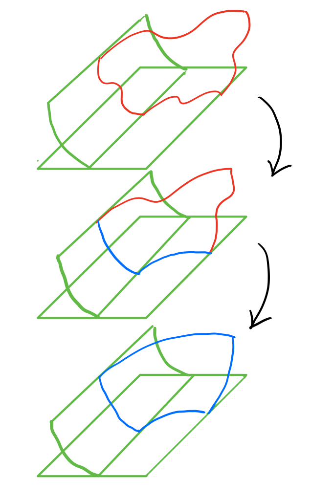
Refer to caption
Figure 3.5. The strategy of the proof: inductively normalize tangencies.

To pursue this argument, we need the following control over primary tangencies.

Lemma 3.34.

Fix 0≤k<j≤n−10\leq k<j\leq n-1.

We have

τ⁡(τ⁡(Υn,Γkn),τ⁡(Γjn,Γkn))⊃τ⁡(Υn,Γjn)∩τ⁡(Γjn,Γkn)\textstyle{\tau(\tau(\Upsilon_{n},{}^{n}\Gamma_{k}),\tau({}^{n}\Gamma_{j},{}^{n}\Gamma_{k}))\supset\tau(\Upsilon_{n},{}^{n}\Gamma_{j})\cap\tau({}^{n}\Gamma_{j},{}^{n}\Gamma_{k})}

Moreover, when k=n−2k=n-2, the tangency of τ⁡(Υn,Γn−2n)\tau(\Upsilon_{n},{}^{n}\Gamma_{n-2}) and τ⁡(Γn−1n,Γn−2n)\tau({}^{n}\Gamma_{n-1},{}^{n}\Gamma_{n-2}) is nondegenerate.

Proof.

We will assume k>0k>0 and leave the case k=0k=0 as an exercise.

Fix a point

y∈τ⁡(Υn,Γjn)∩τ⁡(Γjn,Γkn)\textstyle{y\in\tau(\Upsilon_{n},{}^{n}\Gamma_{j})\cap\tau({}^{n}\Gamma_{j},{}^{n}\Gamma_{k})}

In particular y∈Υny\in\Upsilon_{n} and so y=π⁡(y~)y=\pi(\tilde{y}) for some y~∈Λnn\tilde{y}\in{}^{n}\Lambda_{n}. Recall Λnn=⋃εΛεnn{}^{n}\Lambda_{n}=\bigcup_{\varepsilon}{}^{n}\Lambda_{n}^{\varepsilon} and so y~∈Λεnn\tilde{y}\in{}^{n}\Lambda_{n}^{\varepsilon}, for some ε\varepsilon.

Note y∈τ⁡(Υn,Γjn)y\in\tau(\Upsilon_{n},{}^{n}\Gamma_{j}) implies y~\tilde{y} is in the closure of the clean codimension one intersection of Λnn,Λjn{}^{n}\Lambda_{n},{}^{n}\Lambda_{j}.

By Corollary 3.26, this locus intersects Λεnn{}^{n}\Lambda_{n}^{\varepsilon} precisely along Λnεn∩Λjεn{}^{n}\Lambda^{\varepsilon}_{n}\cap{}^{n}\Lambda^{\varepsilon}_{j} and so y~∈Λεjn\tilde{y}\in{}^{n}\Lambda_{j}^{\varepsilon}.

Similarly, note y∈τ⁡(Γjn,Γkn)y\in\tau({}^{n}\Gamma_{j},{}^{n}\Gamma_{k}) implies y~\tilde{y} is in the closure of the clean codimension one intersection of Λjn,Λkn{}^{n}\Lambda_{j},{}^{n}\Lambda_{k}. By Corollary 3.26, this locus intersects Λεjn{}^{n}\Lambda_{j}^{\varepsilon} precisely along Λjεn∩Λkεn{}^{n}\Lambda^{\varepsilon}_{j}\cap{}^{n}\Lambda^{\varepsilon}_{k} and so y~∈Λεkn\tilde{y}\in{}^{n}\Lambda_{k}^{\varepsilon}.

Thus altogether y~∈Λnεn∩Λjεn∩Λkεn=(Λnεn∩Λkεn)∩(Λjεn∩Λkεn)\tilde{y}\in{}^{n}\Lambda^{\varepsilon}_{n}\cap{}^{n}\Lambda^{\varepsilon}_{j}\cap{}^{n}\Lambda^{\varepsilon}_{k}=({}^{n}\Lambda^{\varepsilon}_{n}\cap{}^{n}\Lambda^{\varepsilon}_{k})\cap({}^{n}\Lambda^{\varepsilon}_{j}\cap{}^{n}\Lambda^{\varepsilon}_{k}).

By Corollary 3.26, the intersections Λnεn∩Λkεn{}^{n}\Lambda^{\varepsilon}_{n}\cap{}^{n}\Lambda^{\varepsilon}_{k} and Λjεn∩Λkεn{}^{n}\Lambda^{\varepsilon}_{j}\cap{}^{n}\Lambda^{\varepsilon}_{k} are closures of clean codimension one intersections, hence their projections lie in the primary tangencies τ⁡(Υn,Γkn)\tau(\Upsilon_{n},{}^{n}\Gamma_{k}) and τ⁡(Γjn,Γkn)\tau({}^{n}\Gamma_{j},{}^{n}\Gamma_{k}). Moreover, Λnεn∩Λkεn{}^{n}\Lambda^{\varepsilon}_{n}\cap{}^{n}\Lambda^{\varepsilon}_{k} and Λjεn∩Λkεn{}^{n}\Lambda^{\varepsilon}_{j}\cap{}^{n}\Lambda^{\varepsilon}_{k} intersect along their primary tangency. Since π\pi restricted to Λkn{}^{n}\Lambda_{k} has no critical points, the projection of this primary tangency is again a primary tangency. Hence y∈τ⁡(τ⁡(Υn,Γkn),τ⁡(Γjn,Γkn))y\in\tau(\tau(\Upsilon_{n},{}^{n}\Gamma_{k}),\tau({}^{n}\Gamma_{j},{}^{n}\Gamma_{k})), proving the asserted containment.

We leave the nondegeneracy of the case k=n−2k=n-2 to the reader. ∎

Now we are ready to inductively normalize the primary tangencies.

Lemma 3.35.

Fix 0≤k<n−10\leq k<n-1.

Suppose

τ⁡(Υn,Γjn)=τ⁡(Γnn,Γjn)\textstyle{\tau(\Upsilon_{n},{}^{n}\Gamma_{j})=\tau({}^{n}\Gamma_{n},{}^{n}\Gamma_{j})}j>k\textstyle{j>k}

Then there exists a diffeomorphism ψ:ℝn+1→ℝn+1\psi:{\mathbb{R}}^{n+1}\to{\mathbb{R}}^{n+1} preserving Υ′=⋃i=0n−1Γin\Upsilon^{\prime}=\bigcup_{i=0}^{n-1}{}^{n}\Gamma_{i} such that

τ⁡(ψ⁡(Υn),Γjn)=τ⁡(Γnn,Γjn)\textstyle{\tau(\psi(\Upsilon_{n}),{}^{n}\Gamma_{j})=\tau({}^{n}\Gamma_{n},{}^{n}\Gamma_{j})}j≥k\textstyle{j\geq k}

Moreover, when k≠n−2k\not=n-2, the diffeomorphism is an isotopy.

Proof.

We will assume k<n−3k<n-3. We leave the elementary cases k=n−2,n−3k=n-2,n-3 to the reader. They can be deduced from the parametric versions of the cases n=0,1n=0,1 presented in 3.5.1, 3.5.2 respectively.

Throughout what follows, we use the projection ℝn+1→ℝn{\mathbb{R}}^{n+1}\to{\mathbb{R}}^{n} to identify Γkn=ℝn{}^{n}\Gamma_{k}={\mathbb{R}}^{n}.

On the one hand, we have

τ⁡(Γjn,Γkn)=ℝk×Γj−k−1n−k−1\textstyle{\tau({}^{n}\Gamma_{j},{}^{n}\Gamma_{k})={\mathbb{R}}^{k}\times{}^{n-k-1}\Gamma_{j-k-1}}k<j<n\textstyle{k<j<n}

On the other hand, by Lemma 3.34 and assumption, we have

τ⁡(τ⁡(Υn,Γkn),τ⁡(Γjn,Γkn))=τ⁡(Υn,Γjn)∩Γkn=τ⁡(Γnn,Γjn)∩Γkn\textstyle{\tau(\tau(\Upsilon_{n},{}^{n}\Gamma_{k}),\tau({}^{n}\Gamma_{j},{}^{n}\Gamma_{k}))=\tau(\Upsilon_{n},{}^{n}\Gamma_{j})\cap{}^{n}\Gamma_{k}=\tau({}^{n}\Gamma_{n},{}^{n}\Gamma_{j})\cap{}^{n}\Gamma_{k}}k<j<n\textstyle{k<j<n}

Hence within Γkn=ℝn{}^{n}\Gamma_{k}={\mathbb{R}}^{n}, the loci τ⁡(Υn,Γkn)\tau(\Upsilon_{n},{}^{n}\Gamma_{k}) and τ⁡(Γnn,Γkn)\tau({}^{n}\Gamma_{n},{}^{n}\Gamma_{k}) have the same tangencies with

τ⁡(Γjn,Γkn)=ℝk×Γj−k−1n−k−1\textstyle{\tau({}^{n}\Gamma_{j},{}^{n}\Gamma_{k})={\mathbb{R}}^{k}\times{}^{n-k-1}\Gamma_{j-k-1}}k<j<n\textstyle{k<j<n}

Thus Proposition 3.29 and Proposition 3.30 provide a time-dependent vector field of the form

vt=ht∑i=k+1n−112ixi∂xi\textstyle{v_{t}=h_{t}\sum\limits_{i=k+1}^{n-1}\frac{1}{2^{i}}x_{i}\partial_{x_{i}}}

generating an isotopy φ:ℝn−k→ℝn−k\varphi:{\mathbb{R}}^{n-k}\to{\mathbb{R}}^{n-k} satisfying

φ⁡(τ⁡(Υn,Γkn))=τ⁡(Γnn,Γkn)\textstyle{\varphi(\tau(\Upsilon_{n},{}^{n}\Gamma_{k}))=\tau({}^{n}\Gamma_{n},{}^{n}\Gamma_{k})}

In addition, the function hth_{t}, hence vector field vtv_{t}, is divisible by the product ∏j=k+1n−1hn,j,\prod_{j=k+1}^{n-1}h_{n,j}, and thus φ\varphi preserves its zero-locus.

Let us complete vtv_{t} to the vector field

Vt=ht∑i=0n−112ixi∂xi\textstyle{V_{t}=h_{t}\sum\limits_{i=0}^{n-1}\frac{1}{2^{i}}x_{i}\partial_{x_{i}}}

and consider the isotopy ψ:ℝn+1→ℝn+1\psi:{\mathbb{R}}^{n+1}\to{\mathbb{R}}^{n+1} generated by VtV_{t}.

Then ψ\psi satisfies

ψ⁡(τ⁡(Υn,Γkn))=τ⁡(Γnn,Γkn)\textstyle{\psi(\tau(\Upsilon_{n},{}^{n}\Gamma_{k}))=\tau({}^{n}\Gamma_{n},{}^{n}\Gamma_{k})}

It also preserves Γin{}^{n}\Gamma_{i}, for 0≤i≤n−10\leq i\leq n-1, as well as τ⁡(Υn,Γjn)=τ⁡(Γnn,Γjn)\tau(\Upsilon_{n},{}^{n}\Gamma_{j})=\tau({}^{n}\Gamma_{n},{}^{n}\Gamma_{j}), for j>kj>k. In addition, it preserves

τ⁡(Γjn,Γkn)=ℝk×Γj−k−1n−k−1\textstyle{\tau({}^{n}\Gamma_{j},{}^{n}\Gamma_{k})={\mathbb{R}}^{k}\times{}^{n-k-1}\Gamma_{j-k-1}}k<j<n\textstyle{k<j<n}

since this is the zero-locus of hn,jh_{n,j}. ∎

Finally, let us use the lemma to complete the inductive step of the proof of Theorem 3.27 as outlined above. Suppose for some 0<k≤n−10<k\leq n-1, we have moved Υn\Upsilon_{n}, while preserving Υ′\Upsilon^{\prime}, so that we have the sought-after primary tangencies

τ⁡(Υn,Γjn)=τ⁡(Γnn,Γjn)\textstyle{\tau(\Upsilon_{n},{}^{n}\Gamma_{j})=\tau({}^{n}\Gamma_{n},{}^{n}\Gamma_{j})}j>k\textstyle{j>k}

Then using Lemma 3.35, we can move Υn\Upsilon_{n}, while preserving Υ′\Upsilon^{\prime}, so that we have the sought-after primary tangencies

τ⁡(Υn,Γjn)=τ⁡(Γnn,Γjn)\textstyle{\tau(\Upsilon_{n},{}^{n}\Gamma_{j})=\tau({}^{n}\Gamma_{n},{}^{n}\Gamma_{j})}j≥k\textstyle{j\geq k}

Proceeding in this way, we arrive at k=0k=0, where all primary tangencies have been normalized. Now a final application of Proposition 3.29 and Proposition 3.30 move Υn\Upsilon_{n} to Γnn{}^{n}\Gamma_{n}, while preserving Υ′\Upsilon^{\prime}, and thus complete the proof of Theorem 3.27.

3.6. Conclusion of the proof

We are now ready to prove Proposition 3.6. As a consequence we establish Theorem 3.5, and since all the above also holds parametrically this also establishes the parametric version Theorem 3.12.

Proof of Proposition 3.6.

Take any point λ\lambda in the front H:=π⁡(Λ)H:=\pi(\Lambda) and let π−1​(λ)={λ1,…,λk}\pi^{-1}(\lambda)=\{\lambda_{1},\dots,\lambda_{k}\}. Let Λ1,…,Λk\Lambda_{1},\dots,\Lambda_{k} be germs of Λ\Lambda at these points of arboreal types (𝒯j,n)(\mathscr{T}_{j},n), n⁡(𝒯j)=njn(\mathscr{T}_{j})=n_{j}. We need to show that the germ of the front HH at λ\lambda is diffeomorphic to the germ of a model front H𝒯H_{\mathscr{T}}, where 𝒯\mathscr{T} is a signed rooted tree obtained from ⨆Tj\bigsqcup T_{j} by adding the root ρ\rho and adjoining it to the roots ρj\rho_{j} of the trees TjT_{j} by edges [ρ​ρj][\rho\rho_{j}]. The signs of all edges of the trees TjT_{j} are preserved, while previously unsigned edges ρj​α\rho_{j}\alpha get a sign ε⁡(ν,L,α)\varepsilon(\nu,L,\alpha), see (1).

We proceed by induction on the number of vertices in the signed rooted tree 𝒯=(T,ρ,ε)\mathscr{T}=(T,\rho,\varepsilon).

The base case of a (𝒜1,m)(\mathscr{A}_{1},m)-front H⊂ℝmH\subset{\mathbb{R}}^{m} is the same geometry as appearing in 3.5.1: any graphical hypersurface H⊂ℝ×ℝm−1H\subset{\mathbb{R}}\times{\mathbb{R}}^{m-1} is isotopic to the germ of the zero-graph {0}×ℝm−1\{0\}\times{\mathbb{R}}^{m-1}.

For the inductive step, fix a rooted tree 𝒯=(T,ρ,ε)\mathscr{T}=(T,\rho,\varepsilon), and as usual set n=|n⁡(𝒯)|n=|n(\mathscr{T})|. Consider a (𝒯,m)(\mathscr{T},m)-front H⊂ℝmH\subset{\mathbb{R}}^{m}, with by necessity m≥nm\geq n.

Fix a leaf vertex β∈ℓ⁡(𝒯)\beta\in\ell(\mathscr{T}), which always exists as long as 𝒯≠𝒜1\mathscr{T}\not=\mathscr{A}_{1}. Consider the smaller signed rooted tree 𝒯′=𝒯∖β\mathscr{T}^{\prime}=\mathscr{T}\setminus\beta, and the corresponding (𝒯′,m)(\mathscr{T}^{\prime},m)-front H′=H∖H̊​[β]⊂ℝmH^{\prime}=H\setminus\mathring{H}[\beta]\subset{\mathbb{R}}^{m}, where H̊​[β]⊂H\mathring{H}[\beta]\subset H is the interior of the smooth piece indexed by β\beta. By induction, we may assume

H′=H𝒯′×ℝm−n+1⊂ℝm\textstyle{H^{\prime}=H_{\mathscr{T}^{\prime}}\times{\mathbb{R}}^{m-n+1}\subset{\mathbb{R}}^{m}}

Thus it remains to normalize the smooth piece H⁡[β]H[\beta].

Let 𝒜β=(Aβ,ρ,εβ)\mathscr{A}_{\beta}=(A_{\beta},\rho,\varepsilon_{\beta}) be the linear signed rooted subtree of 𝒯=(T,ρ,ε)\mathscr{T}=(T,\rho,\varepsilon) with vertices v⁡(Aβ)={α∈v⁡(T)|α≤β}v(A_{\beta})=\{\alpha\in v(T)\,|\,\alpha\leq\beta\}. Set d=v⁡(𝒯)∖v⁡(𝒜β)=n⁡(𝒯)∖n⁡(𝒜β)d=v(\mathscr{T})\setminus v(\mathscr{A}_{\beta})=n(\mathscr{T})\setminus n(\mathscr{A}_{\beta}) to be the complementary vertices.

Consider the (𝒜β,m)(\mathscr{A}_{\beta},m)-front K⊂HK\subset H given by the union K=⋃α∈n⁡(𝒜β)K⁡[α]K=\bigcup_{\alpha\in n(\mathscr{A}_{\beta})}K[\alpha] of the smooth pieces of H⊂ℝmH\subset{\mathbb{R}}^{m} indexed by α∈n⁡(𝒜β)\alpha\in n(\mathscr{A}_{\beta}). Note for 𝒜β′=𝒜β∩𝒯′\mathscr{A}^{\prime}_{\beta}=\mathscr{A}_{\beta}\cap\mathscr{T}^{\prime}, and K′=K∩H′K^{\prime}=K\cap H^{\prime}, we already have

K′=H𝒜β′×ℝm−n+1+d⊂ℝm\textstyle{K^{\prime}=H_{\mathscr{A}_{\beta}^{\prime}}\times{\mathbb{R}}^{m-n+1+d}\subset{\mathbb{R}}^{m}}

and seek to normalize the smooth piece K⁡[β]=H⁡[β]K[\beta]=H[\beta].

Now we can apply Theorem 3.27 to normalize K⁡[β]K[\beta] viewed as the final smooth piece of KK. More specifically, we can apply Theorem 3.27 to normalize K⁡[β]K[\beta] while preserving K′K^{\prime} and viewing the complementary directions ℝm−n+1+d{\mathbb{R}}^{m-n+1+d} as parameters, see Figure 3.6. This insures we preserve H′H^{\prime} and hence do not disturb its already arranged normalization.

This concludes the proof of Proposition 3.6. ∎

Refer to caption
Figure 3.6. Treating the complementary directions as parameters.

References

  • [Ab12] M. Abouzaid, Framed bordism and Lagrangian embeddings of exotic spheres, Annals of Math., 175(2012), 71–185.
  • [AGEN19] D. Alvarez-Gavela, Y. Eliashberg, and D. Nadler, Geomorphology of Lagrangian ridges, arXiv:1912.03439.
  • [AGEN20b] D. Alvarez-Gavela, Y. Eliashberg, and D. Nadler, Positive arborealization of polarized Weinstein manifolds, arXiv:1912.03439.
  • [AGEN22] D. Alvarez-Gavela, Y. Eliashberg, and D. Nadler, Reidemeister moves for positive arboreal skeleta, in preparation.
  • [E18] Y. Eliashberg, Weinstein manifolds revisited, Proc. of Symp. in Pure Math., Amer. Math. Soc., 99(2018), 59–82.
  • [N13] D. Nadler, Arboreal Singularities, arXiv:1309.4122.
  • [N15] D. Nadler, Non-characteristic expansion of Legendrian singularities, arXiv:1507.01513.
  • [St18] L. Starkston, Arboreal Singularities in Weinstein Skeleta, Selecta Mathematica, 24(2018), 4105–4140.