CleftNet: Augmented Deep Learning for Synaptic Cleft Detection from Brain Electron Microscopy
Abstract
Detecting synaptic clefts is a crucial step to investigate the biological function of synapses. The volume electron microscopy (EM) allows the identification of synaptic clefts by photoing EM images with high resolution and fine details. Machine learning approaches have been employed to automatically predict synaptic clefts from EM images. In this work, we propose a novel and augmented deep learning model, known as CleftNet, for improving synaptic cleft detection from brain EM images. We first propose two novel network components, known as the feature augmentor and the label augmentor, for augmenting features and labels to improve cleft representations. The feature augmentor can fuse global information from inputs and learn common morphological patterns in clefts, leading to augmented cleft features. In addition, it can generate outputs with varying dimensions, making it flexible to be integrated in any deep network. The proposed label augmentor augments the label of each voxel from a value to a vector, which contains both the segmentation label and boundary label. This allows the network to learn important shape information and to produce more informative cleft representations. Based on the proposed feature augmentor and label augmentor, We build the CleftNet as a U-Net like network. The effectiveness of our methods is evaluated on both online and offline tasks. Our CleftNet currently ranks #1 on the online task of the CREMI open challenge. In addition, both quantitative and qualitative results in the offline tasks show that our method outperforms the baseline approaches significantly.
Index Terms:
Synaptic cleft detection, electron microscopy, feature augmentation, label augmentationI Introduction
Synapses are fundamental biological structures that transmit signals across neurons. A synapse is composed of several pre-synaptic neurons, a pro-synaptic neuron, and a synaptic cleft between these two types of neurons. [1, 2]. Detecting synaptic clefts is a key step to reconstruct synapses and investigate synaptic functions. Currently, the volume electron microscopy (EM) is recognized as the most reliable technique for reconstruction of neural circuits [3, 4, 5, 6, 7, 8]. It can provide 3D EM images with high resolution and sufficient details for synaptic cleft detection and synaptic structure analysis [9, 10].
The manual annotation of synaptic clefts is time-consuming and requires heavy labor from domain experts [11]. This raises the need of constructing computational models to automatically detect synaptic clefts from EM images. Machine learning approaches [1, 12, 9, 13] have been employed to learn relationships between EM images and the annotated clefts. Then for any newly obtained EM image, the synaptic clefts it contains could be directly predicted by the trained models. Earlier studies [1, 12] employ traditional machine learning methods for synaptic cleft detection. These methods require carefully-designed features based on the prior knowledge of synapses and EM images.
With the rapid development of deep learning, recent methods [9, 13] automatically learn features from EM images using deep neural networks. Thus, hand-crafted features are avoided and models can be learned end-to-end. Importantly, synaptic cleft detection is formulated as an image dense prediction problem, where each voxel in the input volume is predicted as a cleft voxel or not. There exist several deep architectures for the dense prediction of biological images [14, 15, 16, 17, 18, 19], among which networks based-on the U-Net architecture [16, 20, 21, 22] are shown to achieve the best performance. Existing studies [9, 13] apply vanilla U-Nets to cleft detection and obtain the state-of-the-art results. However, they do not consider the unique properties of clefts, e.g., morphological patterns and geometrical shapes of clefts.
In this work, we propose the CleftNet, a novel deep learning model for improving synaptic cleft detection from brain EM images. Our CleftNet contains two novel components, known as the feature augmentor (FA) and the label augmentor (LA), to augment features and labels by considering and learning important properties of clefts. The feature augmentor is inspired by the attention mechanisms [23, 24]. The feature representation of each output position in the FA is dependent on features of all positions in the input. Hence, global information is captured effectively to improve cleft features. Importantly, a trainable query tensor is used to learn common morphological patterns of all synaptic clefts. The query is fully trainable and updated by all input EM images. Thus, it can capture common patterns and learn topological structures in clefts, leading to augmented feature representations. Note that our proposed FA is flexible in terms of generating outputs of different sizes. Thus, it can simulate any commonly-used operations, like pooling, convolution, or deconvolution, and can be easily integrated into any deep neural network.
In addition to augmenting features using the FA, we propose the label augmentor to augment labels for voxels. Existing methods mainly use original segmentation labels, which is demonstrated to be biased towards learning image textures while ignoring shape information [25, 26]. However, such information is important to circuit reconstruction based on biological images [13]. To this end, We proposed the LA to augment the label of each voxel from a scalar to a vector, which contains the segmentation label and the boundary label for the voxel. By doing this, the network is encouraged to learn both the texture and shape information from inputs, leading to more informative representations. Finally, we build the CleftNet, a U-Net like network integrating the proposed feature augmentors and label augmentors. We replace all the pooling layers, deconvolution layers, and the bottom block with the appropriately sized FAs to generate augmented features. A novel loss function based on the LA is used in the CleftNet for learning more powerful cleft representations.
We conduct comprehensive experiments to evaluate our methods. First, we apply our methods to the MICCAI Challenge on Circuit Reconstruction from Electron Microscopy Images (CREMI). Our CleftNet now ranks #1 on the synaptic cleft detection task of the CREMI open challenge. Next, we compare our methods with several baseline methods on both the validation set and the test data. Quantitative and qualitative results show that our methods achieve significant improvements over the baselines. In addition, we conduct ablation studies to demonstrate the effectiveness of the important network components including the FA, LA and the learnable query. Overall, our contributions are summarized as below:
- •
We propose the feature augmentor that improves cleft features through fusing global information from inputs and learning shared patterns in clefts. It can generate outputs with varying dimensions and can be adapted to any deep network with high flexibility.
- •
We design the label augmentor that augments the label for each voxel from a scalar to a vector. The LA enables the network to prioritize the learning of shape information, which is important for identifying synaptic clefts.
- •
We develop the CleftNet, an augmented deep learning method considering and learning specific morphological patterns and shape information in clefts. CleftNet generates improved cleft representations by incorporating the proposed feature augmentor and label augmentor.
- •
CleftNet is the new state-of-the-art model for synaptic cleft detection. It not only ranks #1 on the online task of the CREMI open challenge, but also outperforms other baseline methods significantly on offline tasks.
II Related Work
II-A Synaptic Cleft Detection
Machine learning methods have been explored for synaptic cleft detection. Earlier studies [1, 12] employ traditional machine learning methods with carefully-designed features. The work in [1] designs features for synapses by considering similar texture cues shared by clefts. The constructed features are then taken by an AdaBoost-based classifier to identify synapses and clefts. The work in [12] applies a random-forest classifier to hand-crafted features that constructed based on the geometrical information in EM volumes. Recently, deep learning methods [9, 13] are used to automatically learn features from EM images. Synaptic cleft detection is formulated as an image dense prediction problem in these methods. The work in [9] uses the 3D residual U-Net [27] to detect cleft voxels from a newly obtained large EM dataset. The misalignment issue of adjacent patches is tackled by designing a training strategy that is robust to misalignments. The work in [13] employs the vanilla 3D U-Net with an auxiliary task to detect clefts and uses the CREMI [28] dataset. Both approaches apply well-studied deep architectures and obtain state-of-the-art detection performance on the used datasets. In this work, we propose a novel deep model, known as CleftNet, to improve synaptic cleft detection by augmenting cleft features and labels of clefts.

II-B Attention on Images
We summarize the attention-based methods on images in this section. Generally, there exist two categories of attention methods for images in literature; those are, gated-attention (GateAttn) methods and self-attention (SelfAttn) methods. We start by defining annotations for clear illustration. Given an input image tensor , we convert it to a matrix following appropriate modes as introduced in [29], where denotes the spatial dimensions, and denotes the channel dimension. For instance, if the input is a 3D image, where , and denote the depth, height, and the width, respectively.
II-B1 Gated-attention Methods
The GateAttn aims at selecting important features from inputs using a trainable vector. The selection could be conducted along the spatial direction, namely spatial-wise attention (SWA), as used in the spatial attention module in CBAM [30] and the attention U-Net [23]. In the SWA, the matrix could be treated as a set of vectors as , where each is a vector representation for the pixel or voxel , and . If the selection is performed along the channel direction, it is known as the channel-wise attention (CWA) and is used in the channel attention module in CBAM [30] and the squeeze and excitation networks [31]. We use the matrix in CWA and it could be treated as a set of vectors as , where each is a vector representation for the channel , and .
Let and denote the learnable vectors for the SWA and the CWA. The corresponding importance vectors and are computed as
| (1) | ||||
where denotes the element-wise softmax operation. Essentially, each in is the inner product of and , which serves as the important score for . Similarly, the important score for is computed as the inner product of and . Finally, in SWA, each is scaled by its important score , resulting in the output matrix as a set of vectors as . Similarly, in CWA, the generated matrix could be treated as . Essentially, SWA imposes an importance score for each pixel/voxel vector representation, and CWA applies an importance score for each channel vector representation. The obtained or can be converted back to the output tensor that has the same dimensions as the input . Importantly, the GateAttn is used to highlight important pixels/voxels or channels, but fails in capturing global information to the output. In addition, using a trainable vector constraints the network’s capability to learn complicated patterns, such as the common morphological patterns shared by all clefts.
II-B2 Self-attention Methods
The SelfAttn is firstly introduced in the work [24] and then applied to images [32] and videos [33]. It first performs linear transformation on the three times and generates three tensors; those are, the query , the key , and the value . These three tensors are converted to three matrix , , and along the appropriate modes [29]. Each matrix has the dimensions of same as . SelfAttn is then performed as
| (2) |
where denotes the column-wise softmax operation. is then converted back to the tensor that has the same dimensions as . By performing SelfAttn, Each pixel/voxel feature in the output is dependent on features of all the pixels/voxels in the input . To this end, SelfAttn is used to capture long-range dependencies and aggregate global information from inputs. However, all the three tensors , , and are generated from inputs, making them input-dependent, which may not able to capture the common patterns shared by all clefts. In addition, SelfAttn preserves the dimensions from inputs, which leads to its nature of low flexibility. For instance, we can only replace a convolution with a stride of 1 with SelfAttn. It can not simulate other operations that change the input dimensions, such as pooling or deconvolution.
III The Proposed Methods
III-A Feature Augmentation
The self-attention mechanism [24, 33] has achieved great success in various domains, including natural language processing [34, 35] and computer vision [21, 22, 36]. Based upon the self-attention mechanism, we propose a novel method, known as the feature augmentor (FA), to improve cleft feature representations. Our proposed FA not only aggregates global information from the whole feature space of inputs, but also captures shared patterns of all synaptic clefts in the whole dataset, thereby leading to augmented and improved feature representations.
An illustration of our proposed FA is provided in Figure 1. Formally, let denote the input tensor to the FA, where is the depth, is the height, is the width, and is the number of feature maps. We first generate the key tensor and the value tensor from the input tensor by performing two separate 3D convolutions, each of which has a kernel size of and a stride of . The used convolutions retain the spatial sizes of the input tensor but generate varying numbers of feature maps. Assuming the first convolution above produces feature maps, thus, we have . Similarly, we obtain assuming the second convolution generates feature maps. Note that and are both generated from , hence, they are input-dependent.
Next, we consider the query tensor in our proposed FA. Existing studies [21, 22, 36] use the same strategies to generate as and , making it to be input-dependent. In this work, we instead formulate as a learnable tensor containing free parameters, where , , , and denote the depth, height, width, and the number of feature maps, respectively. The parameters in are randomly initialized and trained along with other parameters during the whole learning process. Note that , , can be any positive integers, but needs to be equal to as required by the attention mechanism.
The main purpose of using a learnable query is to capture shared patterns of all synaptic clefts. Even though different synaptic clefts exhibit distinct shapes, they share common morphological patterns. Such patterns are important for learning structural topology and improving cleft feature representations. Existing studies [21, 22, 36] obtain the query tensor by imposing a linear transformation on the input tensor . However, they suffer from two limitations when learning cleft features. First, the input-dependent query fails to capture the common patterns shared by all clefts. In addition, the shared patterns are complicated, and it is difficult to explicitly capture them by performing a linear transformation on the input. To this end, we use a trainable query to automatically learn such complicated and shared patterns. As is shared and updated by all input volumes in the dataset, it is expected to grasp common patterns and help to augment cleft features.
After obtaining the tensors , , and , we perform attention by first converting them to three matrices. Formally, we have
| (3) | ||||
where denotes the mode-4 matricization of an input tensor [29]. The attention is then performed as
| (4) |
where denotes the column-wise softmax operation. The is then converted back to the tensor along mode-4 [29]. Another 3D convolution is performed on to produce to match the number of feature maps of the input . Then the final output of the proposed FA is computed as
| (5) |
where denotes the residual operations that directly map the input to the output with the purpose of reusing features and accelerating training [37]. It is obvious that the depth, height, and width of are determined by . Theoretically, , , and can be any positive integers. In practice, we consider three scenarios to be corresponding to other commonly-used operations. For instance, we set to correspond with a pooling or a convolution with a stride of ; we set to match up with a deconvolution with a stride of 2; we can also preserve the spatial dimensions from the input to simulate a convolution with a stride of 1. For the residual operations, accordingly, we simply use a max pooling, a trilinear interpolation with a factor of 2, and an identical mapping for these three scenarios.
Generally, the matrix in Eq. 4 can be treated as a set of query vectors , and it is similar to , and the produced . enables each query to attend each key vector , generating an attention map as a matrix , where , and . This matrix is further normalized by performing the column-wise softmax operation. Next, by multiplying at the left side, each output vector in is obtained as a weighted sum of all the value vectors in , with each scaled by the weight in the attention map matrix. By doing this, the feature vector of each voxel in the tensor is dependent on feature vectors of all the voxels in the input. Hence, global information from the whole feature space of the input is captured effectively. In addition, we use a learnable query tensor to automatically learn shared pattern features of all synaptic clefts. The query is randomly initialized and trained during the whole learning process. As is shared and updated by all input volumes, it is expected to grasp common patterns and shape structural relationships in clefts, thereby leading to augmented feature representations.
III-B Label Augmentation
Deep neural networks (DNNs) have achieved state-of-the-art performance on the tasks of dense prediction for 3D images [20, 38, 22] Existing methods mainly perform voxel-wise classification and the label information only contains the category for each voxel. In this work, we propose the label augmentor (LA) to augment labels and explicitly consider shape information of clefts.
Generally, an image contains color, shape, and texture information. These information is combined together to DNNs for pixel/voxel-wise classification [25, 39]. The work in [26] demonstrates that DNNs have strong biases towards learning textures but pay little attention to shapes. In biological-image analysis, however, manual annotations from domain experts are usually conducted with the prior knowledge of boundary and shape identification. For instance, segmenting clefts from tissue volumes would entail following cleft boundaries and consequently narrowing the region of interest. Hence, it is natural to leverage shape information to enhance the capability of the networks. To this end, we propose to prioritize the learning of boundary information by augmenting labels. Specifically, for each voxel, we augment its label from a scalar to a vector, which consists of both the segmentation category and the corresponding boundary information. The proposed label augmentor enables the multi-task learning that captures ample information from input EM images.
There exist several methods to compute and incorporate boundary information [25, 40, 41, 42]. In this work, we follow the thread and use tanh distance map (TDM) to compute the tanh of the Euclidean distance of each voxel from the nearest boundary voxel [43]. Formally, let denote the set of cleft voxels for one synaptic cleft, and let represent the set of boundary voxels for this synaptic cleft. Then the tanh distance map, , is defined as
| (6) |
where is the index of any voxel in the input volume, denotes the Euclidean distance for any two voxels, and is the element-wise tanh operation. Apparently, is in the range of based on the definition. Essentially, TDM reveals how each voxel contributes to the shape of the corresponding cleft. Let denote the original segmentation category of the voxel . To this end, we augment the label for each voxel to a vector .
We use the same network to produce the outputs of two streams corresponding to two labels, and the parameters are shared across both streams. By doing this, the network is forced to learn rich texture and shape information, thereby leading to more powerful representations. Let indicate the voxel is a cleft voxel. We use the weighted binary cross-entropy loss for the segmentation steam as
| (7) |
where is the ratio of non-cleft voxels to all voxels in the volume, is the probability of the predicted class for the voxel , and , are the sets of indexes of voxels whose segmentation labels are clefts, non-clefts, respectively. As the data is imbalanced and the non-clefts are overwhelmingly dominant in the volume, is close to one while is close to zero. Intuitively, we use larger penalties for cleft voxels in the loss function to tackle the imbalance issue.
Essentially, the segmentation stream is a voxel-wise classification problem, while the boundary stream is a voxel-wise regression problem. We use the weighted L2 loss for the boundary stream as
| (8) |
where is the ratio of voxels whose boundary labels are larger than zero to all voxels in the volume, is the predicted boundary distance of the voxel , and , are the sets of indexes of voxels whose boundary labels are positive, and zeros, respectively.
We augment the label of each voxel to a vector , and the boundary label is computed based on the provided segmentation label . Importantly, there exists correspondence between these two scalars. Specifically, the segmentation label is in line with the boundary label , and corresponds to . By augmenting labels and employing the same network with weight sharing, the texture and shape information are jointly learned together in the training phase. However, there may still exist mismatch in the predicted segmentation map and shape map. Here, we propose a coherence loss as a regularizer as
| (9) |
where , and denote the sets of voxels whose predicted boundary values are positive, and non-positive, respectively. Intuitively, we impose a penalty to voxel if the two predicted values and are not consistent with each other. Specifically, there are two terms in Eq. 9. The former penalizes the voxel whose predicted boundary value is positive while the predicted segmentation value is zero. We use the function to impose heavier penalties for the voxels close to the boundary. For the latter, the voxel is penalized if the predicted boundary value is zero but the predicted segmentation value is one. Note that ranges from to in the former. Correspondingly, we use to produce a probability that also ranges from to in the latter.
The final loss is computed as the weighted sum of the above three loss functions as
| (10) |
where the weights and are hyper-parameters. By doing this, the network is forced to learn high-level patterns for both the segmentation label and boundary label. As a result, shape information is explicitly considered in LA to benefit synaptic cleft detection.
III-C CleftNet
Deep architectures have been intensively studied for dense prediction of biological images [15, 16, 21], among which networks based on the U-Net architecture are shown to achieve superior performance [16, 20, 21]. Essentially, the U-Net consists of an encoder and a decoder, which are connected by the bottom block and several skip connections. In this work, we propose the CleftNet, a U-Net like network with the proposed feature augmentors and label augmentors, for improving synaptic cleft detection from EM images. Specifically, we replace all the downsampling layers in the encoder, all the upsampling layers in the decoder, and the bottom block of the vanilla U-Net with the corresponding FAs as introduced in Section III-A. For example, we replace a downsampling layer with a FA where the depth, height, and width of the learnable query are all set to be half of those of the input volume. In addition, the residual operation used in this FA is a max pooling. Essentially, The proposed FA augments cleft features by aggregating global information from the whole input volume and capturing commonly shared patterns of all clefts in the whole dataset. By incorporating the proposed LA as described in Section III-B, the CleftNet outputs a vector with two elements for each voxel corresponding to its label vector containing the segmentation label and the boundary label. The final loss function of the CleftNet is the weighted sum of the three loss functions as mentioned in Eq. 10. By doing this, the network is forced to learn both the texture and the shape information for synaptic clefts, thereby leading to more powerful cleft representations.
IV Experimental Studies
IV-A Dataset
We use the dataset from the MICCAI Challenge on Circuit Reconstruction from Electron Microscopy Images (CREMI) [28]. The CREMI dataset was obtained from the adult Drosophila using serial section transmission electron microscopy (ssTEM) with the resolution . The training data is consist of three volumes A, B, and C, each of which has the spatial sizes of . The original segmentation label for the training data indicates whether a voxel is a background voxel or a cleft voxel. There are also three volumes A+, B+, and C+ with the same dimensions as the training volumes in the test data, but the label is not publicly provided. The CREMI challenge requires the submitting of predicted results to conduct unbiased comparisons among different methods. Generally, the data is sparse regarding the ratio of cleft voxels to total voxels.
IV-B Network Settings
Our proposed CleftNet follows the general settings in the 3D U-Net architecture [20] and ResUnet [27] with integrating our proposed FAs and LAs. Both the encoder and decoder contain 4 blocks, and the numbers of output channels of the 4 block are 32, 64, 96, 128, respectively. The bottom block outputs 160 channels. We replace the second convolution block in each of the 9 blocks in the original 3D U-Net architecture [20] with a residual block. By doing this, each of the 9 blocks contains a convolution block, a residual block, and a corresponding FA, sequentially. Each of the 4 used FAs in the encoder serves as a downsampling layer such that the spatial sizes are halved along the depth, height, and the width directions. In the decoder, the FA can be used for performing upsampling and recovering the spatial sizes of inputs. Convolution layers and residual blocks in the encoder and decoder are used for extracting features. Each convolution block is consist of a convolution layer with kernel and stride 1, followed by a batch normalization (BN) layer and ELu with equal to 1 [44]. For each residual block, we employ the original version of ResNets in [45] that addition is performed after the second BN layer and before the second Elu. The output block integrates our proposed LA and generates two channels for both the textual and shape learning. The weights in Eq. 10 are , , respectively.
IV-C Training and Inference
Each of the three volumes A, B, C in the training data contains 125 slices. We use the first 100 slices of all the A, B, C as the training set. The last 25 slices of A, B, C are used as the validation set. In this way, the training set contains three volumes with sizes of , while the validation set contains three volumes with sizes of .
We compute the augmented label vector based on the original segmentation label for each voxel of the input volumes. The input sizes of the network are set to be . During training, a 3D patch with sizes is randomly cropped from the any of the three volumes as input to the network to train the weights. During inference, we first perform prediction for each patch and then stack all the predicted patches together to generate the final prediction map for each volume. As the data is sparse, we further tackle the imbalance issue by counting the number of cleft voxels in an input patch. Specifically, we reject a patch with a high probability of 95% if it contains less than 200 cleft voxels. Our data augmentation techniques include rotation with probability 0.5, flip with probability 0.5, and grayscale with probability 0.2. We set the batch size to be 16 using four NVIDIA GeForce RTX 2080 Ti GPUs. To optimize the model, we employ the Adam optimizer [46] with a learning rate of 0.001. All hyper-parameters are tuned on the validation set. We run iterations in total, and inference on the validation set is performed per 100 iterations.
After obtaining the optimized model, we conduct inference on the test data, which contains three volumes A+, B+, and C+ with sizes of . We use the same input patch sizes and generate predicted patches then stack them together as the final predictions. As the ground truth of the test data is not publicly provided, we submitted the predictions to CREMI open challenge to compute the model performance.
| Rank | Group | Model | CREMI-score() |
|---|---|---|---|
| 1 | DIVE | CleftNet | 57.73 |
| 4 | CleftKing | CleABC1 | 58.02 |
| 6 | lbdl | lb_thicc | 59.04 |
| 9 | 3DEM | BesA225 | 59.34 |
| 15 | SDG | Unet2 | 63.92 |
IV-D Metrics
As data is imbalanced regarding the ratio of cleft voxels to total voxels in three volumes, we use F1-score, AUC, and CREMI-score for evaluation. Specifically, AUC represents area under the ROC curve, where the ROC curve is created by plotting true positive rate (TPR) against the false positive rate (FPR). Formally, , and , where TP, FN, FP, and TN represent true positive, false negative, false positive, and true negative, respectively. In addition, for the F1-score and CREMI-score, we have
| (11) | ||||
where , and . ADGT represents the average distance of any predicted cleft voxel to the closest ground truth cleft voxel, which is related to FPs in predictions. ADF denotes the average distance of any ground truth cleft voxel to the closest predicted cleft voxel, which is related to FNs in predictions. Essentially, F1-score is the Harmonic mean of recall and precision, and CREMI-score aims at measuring the overall distance between a predicted cleft and a true cleft. Note that CREMI-score is used as the primary ranking metric on the leaderboard of synaptic cleft detection of the CREMI open challenge.
| Model | CREMI-score() | AUC() | F1-score() |
|---|---|---|---|
| SegNet | 72.32 | 0.883 | 0.842 |
| 3D U-Net | 64.27 | 0.875 | 0.837 |
| V-Net | 65.73 | 0.896 | 0.858 |
| ResUnet | 59.64 | 0.909 | 0.874 |
| AttnUnet | 57.34 | 0.914 | 0.878 |
| CleftNet | 50.50 | 0.938 | 0.895 |
| Model | CREMI-score() | F1-score() |
|---|---|---|
| SegNet | 82.46 | 0.794 |
| V-Net | 76.12 | 0.744 |
| 3D U-Net | 75.02 | 0.800 |
| ResUnet | 66.50 | 0.813 |
| AttnUnet | 65.19 | 0.812 |
| CleftNet | 57.73 | 0.831 |
IV-E CREMI Open Challenge Task
The MICCAI Challenge on Circuit Reconstruction from Electron Microscopy Images (CREMI) [28] started from the year of 2016 and has become one of the most well-known open challenges on EM data. There are totally three tasks in the CREMI challenge including neuron segmentation, synaptic cleft detection, and synaptic partner identification. We focus on the task of synaptic cleft detection and the used data is described in Section IV-A. As the label for the test data is not publicly provided, we submitted the predicted results of our CleftNet to the task of synaptic cleft detection of the CREMI challenge, where CREMI-score is used as the primary ranking metric. There are at least 15 groups participating in this task. We summarize the results of the best models for the top 5 groups in Table I. Our best model CleftNet ranks the first with the CREMI-score of 57.73. Note we do not use any model ensemble technique to enhance the performance.
IV-F Comparison with Baselines
We compare our methods with several state-of-the-art architectures including SegNet [47], V-Net [14], 3D U-Net [20], ResUnet [27], and AttnUnet [23]. To ensure fair comparisons, we use similar architectures for all methods, including number of blocks for the encoders and decoders, numbers of output features of each block, etc. In addition, we integrate their official code for specific components (like residual blocks and attention units) to the architectures.
For the validation set, we directly report the computed values for all metrics from the optimized models. The comparison results are provided in Table II. We can observe from the table that our proposed CleftNet consistently outperforms other baseline methods on all the three metrics. Specifically, compared with the best baseline method AttnUnet, CleftNet refines the CREMI-score by a large margin of 6.84, which is a considerable value of 13.5% of our current CREMI-score 50.50. CleftNet reduces the CREMI-score by an average margin of 13.76 when considering all the five baseline methods, which is an incredible percentage of 27.2% of our current score. In addition, CleftNet outperforms the baselines on the other two metrics by average margins of 4.25% in terms of AUC and 3.72% in terms of F1-score. All of these results demonstrate the effectiveness of CleftNet with the proposed feature augmentors and label augmentors.
For the test data, we submitted the predicted volumes from all the optimized models to the CREMI open challenge for evaluation. The results in terms of CREMI-score and F1-score are provided at the CREMI website [28] and summarized in Table III. We draw similar conclusions that CleftNet performs the best on the test data. Specifically, CleftNet outperforms the other five methods by an average margin of 15.33 in terms of CREMI-score, which is 26.6% of the current score 57.73. In addition, CleftNet achieves an average improvement of 3.12% in terms of F1-score. The CREMI open challenge does not provide results for AUC.
| Model | CREMI-score() | AUC() | F1-score() |
|---|---|---|---|
| ResUnet | 59.64 | 0.909 | 0.874 |
| AttnUnet | 57.34 | 0.914 | 0.878 |
| CleftNet w/o FA | 53.37 | 0.922 | 0.883 |
| CleftNet w/o LA | 52.65 | 0.930 | 0.890 |
| CleftNet | 50.50 | 0.938 | 0.895 |
| Model | CREMI-score() | F1-score() |
|---|---|---|
| ResUnet | 66.50 | 0.813 |
| AttnUnet | 65.19 | 0.812 |
| CleftNet w/o FA | 59.11 | 0.820 |
| CleftNet w/o LA | 59.03 | 0.823 |
| CleftNet | 57.73 | 0.831 |
IV-G Ablation Studies
We conduct ablation study to investigate the effectiveness of our proposed components feature augmentor (FA) and label augmentor (LA). We remove the FAs from CleftNet which we denote as CleftNet w/o FA, and we remove the LAs from CleftNet which we denote as CleftNet w/o LA. If we remove both the FAs and LAs then CleftNet would simply become ResUnet. We also include the results of AttnUnet to compare the attention units used in AttnUnet and our proposed FA. Experimental results on the validation set is provided in Table IV. We can observe from the table that CleftNet outperforms ResUnet by large margins of 9.14, 2.7%, and 2.1% in terms of CREMI-score, AUC, and F1-score, respectively. As we use ResUnet as the backbone architecture, the better performance achieved by CleftNet compared with ResUnet indicates the effectiveness of our proposed FA ans LA. In addition, the contribution of FAs can be shown from two comparisons; these are, the better results of CleftNet w/o LA over ResUnet, and the better results of CleftNet over CleftNet w/o FA. Similarly, both the better performances of CleftNet w/o FA over ResUnet and CleftNet over CleftNet w/o LA reveal the effectiveness of LAs.
Notably, the only difference of CleftNet w/o LA from AttnUnet is the use of the FAs rather that the attention units proposed in AttnUnet. Table IV shows that compared with AttnUnet, CleftNet w/o LA induces improvements of 6.99, 2.1%, and 1.6% in terms of CREMI-score, AUC, and F1-score, respectively. This reveals the superior capability of our proposed FA than the attention unit. Essentially, the used attention unit in AttnUnet employs a query vector to highlight more important voxels in the input. The inner product between the query vector and each voxel vector produces a scalar as the importance score of the corresponding voxel. However, it fails to aggregate global context information from the whole input to the output, imposing natural constraints to the network’s capability. In addition, a single vector may not sufficient to store and learn the commonly shared patterns of all clefts in the dataset. Our FA uses a learnable query tensor with high dimensions and generates response of each voxel by considering all the voxels in the input. By doing this, FA not only extracts global information from the whole input volume, but also captures the complicated shared patterns of all clefts in the dataset, leading to augmented and improved cleft features.
We summarize the results on the test data in Table V. For CREMI score, CleftNet w/o LA reduces the score by 7.47 compared with ResUnet, and CleftNet reduces the score by 1.38 compared with CleftNet w/o FA. Both of these demonstrate the contribution of the proposed FA. Similarly, the effectiveness of the LA can be demonstrated by either the improvement of 7.39 induced by CleftNet w/o FA over ResUnet, or the the improvement of 1.30 induced by CleftNet over CleftNet w/o LA. Essentially, we draw consistent conclusions that both the FA and LA make considerable contributions for learning better cleft representations.
| Model | CREMI-score() | AUC() | F1-score() |
|---|---|---|---|
| CleftNet w SelfAttn | 51.98 | 0.932 | 0.894 |
| CleftNet w FA | 50.50 | 0.938 | 0.895 |
IV-H Investigating Different Queries
We investigate the effectiveness of the learnable query in FA compared the input-dependent query in self-attention [24]. The studies [21, 22] use similar strategies to integrate attention-based methods in U-Net, but the query tensor is achieved by performing a linear transformation on the input. By doing this, the query is similar as the key and value that to be input-dependent. For clear illustration, we denote our method as CleftNet w FA, and the methods in [21, 22] as CleftNet w SelfAttn. We conduct experiments to compare these two methods and the results on the validation set are reported in Table VI. We can observe from the table that our method induces slight improvements based on CleftNet w SelfAttn. Specifically, CleftNet w FA outperforms CleftNet w SelfAtt by margins of 1.48, 0.6%, and 0.1% in terms of CREMI-score, AUC, and F1-score, respectively. This indicates that compared with using self-attention, integrating our proposed FA in U-Net generates better cleft representations. The performance improvements are achieved by purely using the learnable query rather than the input-dependent query. Note that our FA can achieve one similar goal as self-attention that capturing global context information. The output response of each voxel fuses information from all the voxels in the whole input volume. However, commonly shared patterns for clefts are complicated, and it is difficult to obtain these patterns by performing a linear transformation on the input. The self-attention used in [21, 22] designs the query to be input-dependent, failing to store and learn complicated inherent patterns shared by all the clefts in the dataset. Instead, in our FA, we design a trainable query tensor to automatically learn such complex patterns during the whole training process and produce better cleft representations.
IV-I Qualitative Results
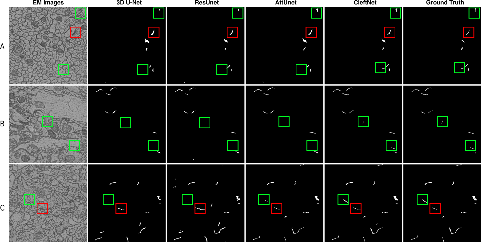
We compare the four best methods among six qualitatively by showing visualization results in Figure 3. Specifically, we compare 3D U-Net, ResUnet, AttnUnet, and CleftNet on the validation set for clear comparisons as the validation set has labels. We show the predicted results for three slices, and each of them is from the volume A, B, and C, respectively. The figure evidently shows that CleftNet generates best cleft predictions among the four methods. Generally, some non-cleft cracks in tissues appear to be similar as clefts, and it is possible that these voxels are predicted as cleft voxels, thereby resulting in false positives. In addition, some clefts have small sizes that the contained voxels can be easily predicted as background voxels, which inducing false negatives. Our CleftNet produces the least false positives or false negatives, generating predictions that are closest to the ground truth. This again demonstrates the effectivenesses of the proposed feature augmentor and label augmentor in CleftNet.
V Conclusion
In this work, we propose a novel deep network, known as CleftNet, for synaptic cleft detection from brain EM images. Our CleftNet is a U-Net like network with the purpose of learning specific properties of synaptic clefts, such as common morphological patterns and shape information of clefts. We achieve this goal by augmenting the network with two network components, the feature augmentor and the label augmentor. The feature augmentor is designed based on the self-attention mechanism but uses a learnable query and generates outputs with arbitrary spatial dimensions. It can not only capture global information from inputs, but also learn complicated morphological patterns shared by all clefts, leading to aumgmented cleft features. The feature augmentor can replace any commonly-used operation, such as convolution, pooling, or deconvolution. Hence, it can be integrated into any deep model with high flexibility. The original label for each input voxel is the segmentation label purely, and we propose the label augmentor to augment it to a vector, which contains both the segmentation label and boundary label. This essentially enables the multi-task learning, and the network is capable of learning both the texture and shape information of clefts, generating more informative representations. We integrate these two components and propose the CleftNet, the new state-of-the-art model for synaptic cleft detection. CleftNet not only ranks first on the online task of the CREMI challenge, but also performs much better than the baseline methods on offline tasks.
References
- [1] C. Becker, K. Ali, G. Knott, and P. Fua, “Learning context cues for synapse segmentation,” IEEE transactions on medical imaging, vol. 32, no. 10, pp. 1864–1877, 2013.
- [2] J. Buhmann, A. Sheridan, S. Gerhard, R. Krause, T. Nguyen, L. Heinrich et al., “Automatic detection of synaptic partners in a whole-brain drosophila em dataset,” bioRxiv, 2019.
- [3] K. Lee, N. Turner, T. Macrina, J. Wu, R. Lu, and H. S. Seung, “Convolutional nets for reconstructing neural circuits from brain images acquired by serial section electron microscopy,” Current opinion in neurobiology, vol. 55, pp. 188–198, 2019.
- [4] R. Li, T. Zeng, H. Peng, and S. Ji, “Deep learning segmentation of optical microscopy images improves 3D neuron reconstruction,” IEEE Transactions on Medical Imaging, vol. 36, no. 7, pp. 1533–1541, 2017.
- [5] A. Fakhry, T. Zeng, and S. Ji, “Residual deconvolutional networks for brain electron microscopy image segmentation,” IEEE Transactions on Medical Imaging, vol. 36, no. 2, pp. 447–456, 2017.
- [6] T. Zeng, B. Wu, and S. Ji, “DeepEM3D: Approaching human-level performance on 3D anisotropic EM image segmentation,” Bioinformatics, vol. 33, no. 16, pp. 2555–2562, 2017.
- [7] A. Fakhry, H. Peng, and S. Ji, “Deep models for brain EM image segmentation: novel insights and improved performance,” Bioinformatics, vol. 32, pp. 2352–2358, 2016.
- [8] D. Wei, Z. Lin, D. Franco-Barranco, N. Wendt, X. Liu, W. Yin et al., “Mitoem dataset: Large-scale 3d mitochondria instance segmentation from em images,” in International Conference on Medical Image Computing and Computer-Assisted Intervention. Springer, 2020, pp. 66–76.
- [9] S. Dorkenwald, N. L. Turner, T. Macrina, K. Lee, R. Lu, J. Wu et al., “Binary and analog variation of synapses between cortical pyramidal neurons,” BioRxiv, 2019.
- [10] S. Dorkenwald, P. J. Schubert, M. F. Killinger, G. Urban, S. Mikula, F. Svara et al., “Automated synaptic connectivity inference for volume electron microscopy,” Nature methods, vol. 14, no. 4, pp. 435–442, 2017.
- [11] Z. Zheng, J. S. Lauritzen, E. Perlman, C. G. Robinson, M. Nichols, D. Milkie et al., “A complete electron microscopy volume of the brain of adult drosophila melanogaster,” Cell, vol. 174, no. 3, pp. 730–743, 2018.
- [12] A. Kreshuk, C. N. Straehle, C. Sommer, U. Koethe, M. Cantoni, G. Knott et al., “Automated detection and segmentation of synaptic contacts in nearly isotropic serial electron microscopy images,” PloS one, vol. 6, no. 10, p. e24899, 2011.
- [13] L. Heinrich, J. Funke, C. Pape, J. Nunez-Iglesias, and S. Saalfeld, “Synaptic cleft segmentation in non-isotropic volume electron microscopy of the complete drosophila brain,” in International Conference on Medical Image Computing and Computer-Assisted Intervention. Springer, 2018, pp. 317–325.
- [14] F. Milletari, N. Navab, and S.-A. Ahmadi, “V-net: Fully convolutional neural networks for volumetric medical image segmentation,” in 2016 fourth international conference on 3D vision (3DV). IEEE, 2016, pp. 565–571.
- [15] J. Long, E. Shelhamer, and T. Darrell, “Fully convolutional networks for semantic segmentation,” in Proceedings of the IEEE conference on computer vision and pattern recognition, 2015, pp. 3431–3440.
- [16] O. Ronneberger, P. Fischer, and T. Brox, “U-net: Convolutional networks for biomedical image segmentation,” in International Conference on Medical image computing and computer-assisted intervention. Springer, 2015, pp. 234–241.
- [17] E. M. Christiansen, S. J. Yang, D. M. Ando, A. Javaherian, G. Skibinski, S. Lipnick et al., “In silico labeling: Predicting fluorescent labels in unlabeled images,” Cell, vol. 173, no. 3, pp. 792–803, 2018.
- [18] P. F. Christ, M. E. A. Elshaer, F. Ettlinger, S. Tatavarty, M. Bickel, P. Bilic et al., “Automatic liver and lesion segmentation in ct using cascaded fully convolutional neural networks and 3d conditional random fields,” in International Conference on Medical Image Computing and Computer-Assisted Intervention. Springer, 2016, pp. 415–423.
- [19] G. Wang, W. Li, M. A. Zuluaga, R. Pratt, P. A. Patel, M. Aertsen et al., “Interactive medical image segmentation using deep learning with image-specific fine tuning,” IEEE transactions on medical imaging, vol. 37, no. 7, pp. 1562–1573, 2018.
- [20] Ö. Çiçek, A. Abdulkadir, S. S. Lienkamp, T. Brox, and O. Ronneberger, “3d u-net: learning dense volumetric segmentation from sparse annotation,” in International conference on medical image computing and computer-assisted intervention. Springer, 2016, pp. 424–432.
- [21] Y. Liu, H. Yuan, Z. Wang, and S. Ji, “Global pixel transformers for virtual staining of microscopy images,” IEEE Transactions on Medical Imaging, vol. 39, no. 6, pp. 2256–2266, 2020.
- [22] Z. Wang, Y. Xie, and S. Ji, “Global voxel transformer networks for augmented microscopy,” Nature Machine Intelligence, 2020.
- [23] O. Oktay, J. Schlemper, L. L. Folgoc, M. Lee, M. Heinrich, K. Misawa et al., “Attention u-net: Learning where to look for the pancreas,” arXiv preprint arXiv:1804.03999, 2018.
- [24] A. Vaswani, N. Shazeer, N. Parmar, J. Uszkoreit, L. Jones, A. N. Gomez et al., “Attention is all you need,” in Advances in Neural Information Processing Systems, 2017, pp. 6000–6010.
- [25] T. Takikawa, D. Acuna, V. Jampani, and S. Fidler, “Gated-scnn: Gated shape cnns for semantic segmentation,” in Proceedings of the IEEE International Conference on Computer Vision, 2019, pp. 5229–5238.
- [26] R. Geirhos, P. Rubisch, C. Michaelis, M. Bethge, F. A. Wichmann, and W. Brendel, “Imagenet-trained cnns are biased towards texture; increasing shape bias improves accuracy and robustness,” in International Conference on Learning Representations (ICLR), 2019.
- [27] Z. Zhang, Q. Liu, and Y. Wang, “Road extraction by deep residual u-net,” IEEE Geoscience and Remote Sensing Letters, vol. 15, no. 5, pp. 749–753, 2018.
- [28] D. B. S. T. E. P. Jan Funke, Stephan Saalfeld, “Miccai challenge oncircuit reconstruction from electron microscopy images,” http://cremi.org/, 2016.
- [29] T. G. Kolda and B. W. Bader, “Tensor decompositions and applications,” SIAM review, vol. 51, no. 3, pp. 455–500, 2009.
- [30] X. Chen, H. Fan, R. Girshick, and K. He, “Improved baselines with momentum contrastive learning,” arXiv preprint arXiv:2003.04297, 2020.
- [31] J. Hu, L. Shen, and G. Sun, “Squeeze-and-excitation networks,” in Proceedings of the IEEE conference on computer vision and pattern recognition, 2018, pp. 7132–7141.
- [32] H. Zhang, I. Goodfellow, D. Metaxas, and A. Odena, “Self-attention generative adversarial networks,” in International conference on machine learning. PMLR, 2019, pp. 7354–7363.
- [33] X. Wang, R. Girshick, A. Gupta, and K. He, “Non-local neural networks,” in Proceedings of the IEEE conference on computer vision and pattern recognition, 2018, pp. 7794–7803.
- [34] Z. Yang, D. Yang, C. Dyer, X. He, A. Smola, and E. Hovy, “Hierarchical attention networks for document classification,” in Proceedings of the 2016 Conference of the North American Chapter of the Association for Computational Linguistics: Human Language Technologies, 2016, pp. 1480–1489.
- [35] Y. Liu, H. Yuan, and S. Ji, “Learning local and global multi-context representations for document classification,” in Proceedings of the 19th IEEE International Conference on Data Mining, 2019, pp. 1234–1239.
- [36] Z. Wang, N. Zou, D. Shen, and S. Ji, “Non-local U-nets for biomedical image segmentation,” in Proceedings of the 34th AAAI Conference on Artificial Intelligence, 2020, pp. 6315–6322.
- [37] K. He, X. Zhang, S. Ren, and J. Sun, “Deep residual learning for image recognition,” in Proceedings of the IEEE conference on computer vision and pattern recognition, 2016, pp. 770–778.
- [38] Y. Chen, H. Gao, L. Cai, M. Shi, D. Shen, and S. Ji, “Voxel deconvolutional networks for 3D brain image labeling,” in Proceedings of the 24th ACM SIGKDD International Conference on Knowledge Discovery and Data Mining, 2018, pp. 1226–1234.
- [39] D. Karimi and S. E. Salcudean, “Reducing the hausdorff distance in medical image segmentation with convolutional neural networks,” IEEE Transactions on medical imaging, vol. 39, no. 2, pp. 499–513, 2019.
- [40] Y. Xue, H. Tang, Z. Qiao, G. Gong, Y. Yin, Z. Qian et al., “Shape-aware organ segmentation by predicting signed distance maps,” in Proceedings of the AAAI Conference on Artificial Intelligence, vol. 34, no. 07, 2020, pp. 12 565–12 572.
- [41] S. Dangi, C. A. Linte, and Z. Yaniv, “A distance map regularized cnn for cardiac cine mr image segmentation,” Medical physics, vol. 46, no. 12, pp. 5637–5651, 2019.
- [42] T. Ni, L. Xie, H. Zheng, E. K. Fishman, and A. L. Yuille, “Elastic boundary projection for 3d medical image segmentation,” in Proceedings of the IEEE Conference on Computer Vision and Pattern Recognition, 2019, pp. 2109–2118.
- [43] G. Borgefors, “Distance transformations in digital images,” Computer vision, graphics, and image processing, vol. 34, no. 3, pp. 344–371, 1986.
- [44] D.-A. Clevert, T. Unterthiner, and S. Hochreiter, “Fast and accurate deep network learning by exponential linear units (elus),” arXiv preprint arXiv:1511.07289, 2015.
- [45] K. He, X. Zhang, S. Ren, and J. Sun, “Identity mappings in deep residual networks,” in European conference on computer vision. Springer, 2016, pp. 630–645.
- [46] D. P. Kingma and J. Ba, “Adam: A method for stochastic optimization,” arXiv preprint arXiv:1412.6980, 2014.
- [47] V. Badrinarayanan, A. Kendall, and R. Cipolla, “Segnet: A deep convolutional encoder-decoder architecture for image segmentation,” IEEE transactions on pattern analysis and machine intelligence, vol. 39, no. 12, pp. 2481–2495, 2017.