跳到论文正文
W Papers独立论文阅读器 arXiv:2101.04254 论文正文 计算阅读时间 · 0%
引用这篇论文根据当前论文元数据生成,正式投稿前建议核对。


License: arXiv.org perpetual non-exclusive license
arXiv:2101.04254v1 [math.CA] 12 Jan 2021

Nonhomogeneous T⁡(1)T(1) Theorem on Product Quasimetric Spaces Note:  The first and second authors are supported by DP170101060. The second author is supported by a Lift-off Fellowship of the Australian Mathematical Society. The third author is supported by DP160100153. The fourth author is partially supported by National Science Foundation DMS grant # 1800057 and Australian Research Council DP 190100970.

Ji Li Email: ji.li@mq.edu.au Address: Department of Mathematics
Macquarie University
NSW 2109, Australia
   Trang T.T. Nguyen Email: trang.t.nguyen1@mymail.unisa.edu.au Address: School of Information Technology and Mathematical Sciences
University of South Australia
Mawson Lakes SA 5095, Australia
   Lesley A. Ward Email: lesley.ward@unisa.edu.au Address: School of Information Technology and Mathematical Sciences
University of South Australia
Mawson Lakes SA 5095, Australia
   Brett D. Wick Email: bwick@wustl.edu Address: Department of Mathematics & Statistics
Washington University – St. Louis
One Brookings Drive, St. Louis, MO USA 63130-4899
Abstract

In this paper, we provide a non-homogeneous T⁡(1)T(1) theorem on product spaces (X1×X2,ρ1×ρ2,μ1×μ2)(X_{1}\times X_{2},\rho_{1}\times\rho_{2},\mu_{1}\times\mu_{2}) equipped with a quasimetric ρ1×ρ2\rho_{1}\times\rho_{2} and a Borel measure μ1×μ2\mu_{1}\times\mu_{2}, which, need not be doubling but satisfies an upper control on the size of quasiballs.

Keywords: 
T⁡(1)T(1) theorem, BMO{\rm BMO}, nonhomogeneous settings, product settings, quasimetric spaces
2010 MSC
Primary 42B20; Secondary 30L99, 43A15

1 Introduction And Statement Of Main Results

The T⁡(1)T(1) Theorem of David and Journé was a ground-breaking result that gave easily-checked criteria for a SIO TT to be bounded from L2​(ℝn)L^{2}(\mathbb{R}^{n}) to L2​(ℝn)L^{2}(\mathbb{R}^{n}) [9]. The name is derived from the fact that these criteria are expressed in terms of the image T⁡(1)T(1) of the constant function 11. Specifically, the T⁡(1)T(1) theorem says that a Calderón–Zygmund operator is bounded on L2​(ℝn)L^{2}(\mathbb{R}^{n}) if and only if T⁡(1)∈BMO⁡(ℝn)T(1)\in{\rm BMO}(\mathbb{R}^{n}); T∗​(1)∈BMO⁡(ℝn)T^{*}(1)\in{\rm BMO}(\mathbb{R}^{n}), and TT satisfies the so-called weak boundedness property. Here T∗T^{*} is the adjoint operator of TT. While incredibly useful, sometimes checking the behavior on T⁡(1)T(1) is not obvious nor direct and instead one wants to test on a function bb that has properties similar to the function 11 (a so called para-accretive function). This extension was also investigated and established by David, Journé and Semmes [10] providing at T⁡(b)T(b) theorem.

The setting of this classical T⁡(1)T(1) theorem of David and Journé is Euclidean space ℝn\mathbb{R}^{n}, equipped with the usual Euclidean metric and Lebesgue measure. In particular, the functions ff that the operator TT acts on are defined on ℝn\mathbb{R}^{n}. Since then, several remarkable results have been obtained along this line of research, further unveiling the strong relationship between the function space BMO{\rm BMO} and the L2L^{2}-boundedness of singular integral operators. In the last twenty years or so, substantial progresses have been made by Tolsa [36, 37, 38, 39], Nazarov–Treil–Volberg [31], in showing that a suitable version of T⁡(1)T(1) theorem also hold without the doubling property of the measure. Specifically, in ℝn\mathbb{R}^{n}, the standard Lebesgue measure can be replaced by a more general measure μ\mu satisfying only the growth condition: for some fixed positive constants CC and d∈(0,n]d\in(0,n],

μ⁡(B⁡(x,r))≤C​rdfor​all​x∈ℝn,r>0.\mu(B(x,r))\leq Cr^{d}\quad{\rm for\ all\ }x\in\mathbb{R}^{n},\ \ r>0.

When it comes to the multi-parameter setting (or product setting), meaning one considers singular integral operators that are invariant under non-isotropic dilations (x1,…,xn)→(δ1​x1,…,δn​xn)(x_{1},\ldots,x_{n})\rightarrow(\delta_{1}x_{1},\ldots,\delta_{n}x_{n}), where xi∈ℝnix_{i}\in\mathbb{R}^{n_{i}}, δi>0\delta_{i}>0, the theory of Calderón and Zygmund for the one-parameter setting does not carry over in a straightforward way. Multiparameter harmonic analysis was introduced in the ’70s and studied extensively in the ’80s, led by S.-Y. A. Chang, R. Fefferman, R. Gundy, J. Journé, J. Pipher, E. Stein and others (see for example [3, 16, 4, 11, 5, 14, 6, 30, 12, 13, 33]). The first T⁡(1)T(1) type theorem for product spaces was proved by Journé [26], where he formulated the assumptions in the language of vector-valued Calderón–Zygmund theory. Later, this has been studied extensively by many authors via Haar expansions, or via product representation theorem, see for example (but not limited to) Pott–Villarroya [34], Martikainen [29], Herrán [19], Ou [32], Li–Martikainen–Vuorinen [28]. Han, Lin and the first author [17] also established the T⁡(1)T(1) theorem on the tensor product of spaces of homogeneous type in the sense of Coifman and Weiss, by using the product version of discrete reproducing formula.

A recent breakthrough was due to Hytönen and Martikainen [24], where they proved a T⁡(1)T(1) theorem on bi-parameter Euclidean spaces ℝn1×ℝn2\mathbb{R}^{n_{1}}\times\mathbb{R}^{n_{2}}, equipped with an upper doubling measure.

Ten year ago, Hytönen [20] set up a more general setting for non-homogeneous analysis on metric spaces (X,d,μ)(X,d,\mu), where (X,d)(X,d) is geometrically doubling, meaning that every ball of radius rr can be covered by at most NN balls of radius r/2r/2, and the measure μ\mu satisfies the so-called upper doubling condition as follows: there exists a dominating function λ:X×ℝ+→ℝ+\lambda:X\times\mathbb{R}_{+}\to\mathbb{R}_{+} and a positive constant CλC_{\lambda} such that for all x∈Xx\in X and r>0r>0,

(i):r→λ⁡(x,r)​is​increasing,(ii):λ⁡(x,2​r)≤Cλ​λ​(x,r),(iii):μ⁡(B⁡(x,r))≤λ⁡(x,r).{\rm(i)}:\ r\to\lambda(x,r)\ {\rm is\ increasing\ },\quad{\rm(ii)}:\ \lambda(x,2r)\leq C_{\lambda}\lambda(x,r),\quad{\rm(iii)}:\ \mu(B(x,r))\leq\lambda(x,r).

Later, many results on the T⁡(b)T(b) and local T⁡(b)T(b) theorems were extended to this general setting. See, for example, [21, 22, 23, 25] and the references therein.

The goal of this paper is to establish a full version of the product T⁡(1)T(1) theorem for Calderón–Zygmund type singular integrals TT on non-homogeneous metric measure spaces setting. This result will marry the multiparameter theory with that of non-homogeneous harmonic analysis.

To be more precise, let (𝒳,ρ,μ):=(X1×X2,ρ1×ρ2,μ1×μ2)(\mathcal{X},\rho,\mu):=(X_{1}\times X_{2},\rho_{1}\times\rho_{2},\mu_{1}\times\mu_{2}) be a non-homogeneous bi-parameter quasimetric space such that for i=1,2i=1,2 we have XiX_{i} is a set, ρi\rho_{i} is a quasimetric on XiX_{i} satisfying the regularity property, μi\mu_{i} is an upper doubling measure on XiX_{i}. On (𝒳,ρ,μ)(\mathcal{X},\rho,\mu), let Ccη​(𝒳)=Ccη​(X1)×Ccη​(X2)C^{\eta}_{c}(\mathcal{X})=C_{c}^{\eta}(X_{1})\times C_{c}^{\eta}(X_{2}), η>0\eta>0 denote the space of continuous functions ff with compact support such that

‖f‖η:=supx1≠y1,x2≠y2|f⁡(x1,x2)−f⁡(y1,x2)−f⁡(x1,y2)+f⁡(y1,y2)|ρ1​(x1,y1)η​ρ2​(x2,y2)η<∞.\|f\|_{\eta}:=\sup_{x_{1}\neq y_{1},x_{2}\neq y_{2}}\frac{|f(x_{1},x_{2})-f(y_{1},x_{2})-f(x_{1},y_{2})+f(y_{1},y_{2})|}{\rho_{1}(x_{1},y_{1})^{\eta}\,\rho_{2}(x_{2},y_{2})^{\eta}}<\infty. (1.1)

We study the operators which satisfy the four Assumptions 2.7–2.10 as in Section 2.4.

Definition 1.1.

A linear operator T:Ccη​(𝒳)→Ccη​(𝒳)′T:C^{\eta}_{c}(\mathcal{X})\rightarrow C^{\eta}_{c}(\mathcal{X})^{\prime} is called a bi-parameter singular integral operator (bi-parameter SIO) if it satisfies Assumptions 2.7–2.10 on size and regularities.

The main result of this paper is as follows.

Theorem 1.2.

Let (𝒳,ρ,μ)(\mathcal{X},\rho,\mu) be a non-homogeneous bi-parameter quasimetric space. Let TT be a bi-parameter SIO as defined above. Assume also that TT satisfies Assumptions 2.16–2.18 on the weak boundedness properties, and S​(1)∈BMOprod​(μ)S(1)\in{\rm BMO}_{\textup{prod}}(\mu) for all S∈{T,T∗,T1,T1∗}S\in\{T,T^{*},T_{1},T^{*}_{1}\}. Then TT extends to a bounded operator on L2​(μ)L^{2}(\mu) and ‖T‖≲1\|T\|\lesssim 1, with a bound depending only on the assumptions and the BMOprod​(μ){\rm BMO}_{\textup{prod}}(\mu) norms of the four S⁡(1)S(1).

Outline of the proof of Theorem 1.2. Inspired by the idea in [31], our goal is divided into three main steps:

  1. Step 1

    Establish Theorem 1.2 under the a priori assumption that the operator norm ‖T‖\|T\| of TT is finite, that is, ‖T‖<∞\|T\|<\infty. See Theorem 1.3.

  2. Step 2

    Establish Theorem 1.2 under the weaker a priori assumption that for all functions f,g∈Ccη​(𝒳)f,g\in C^{\eta}_{\textup{c}}(\mathcal{X}) which are supported on a rectangle R⊂𝒳R\subset\mathcal{X}, we have |⟨T​f,g⟩|≤C⁡(R)​‖g‖L2​(μ)​‖g‖L2​(μ).|\langle Tf,g\rangle|\leq C(R)\|g\|_{L^{2}(\mu)}\|g\|_{L^{2}(\mu)}. See Theorem 1.4.

  3. Step 3

    Establish Theorem 1.2, which the full version of a T⁡(1)T(1) theorem on (𝒳,ρ,μ)(\mathcal{X},\rho,\mu) in which the assumption of a priori boundedness of TT is relaxed.

Initially, it may seem surprising that in Step 1, we assume an a priori bound on the operator norm ‖T‖\|T\|, and then prove that in fact there is then a bound depends (only) on the assumptions and the BMO{\rm BMO} norms of S⁡(1)S(1). The big picture is that in Step 2, this assumption of an a priori bound on ‖T‖\|T\| is weakened, and in Step 3, it is removed entirely.

In fact, the major result of this paper is Step 1. This is because Steps 2 and 3 can always be reduced to Step 1.

We first state the result in Step 1.

Theorem 1.3.

Let (𝒳,ρ,μ)(\mathcal{X},\rho,\mu) be a non-homogeneous bi-parameter quasimetric space. Let TT be a bi-parameter singular integral operator as in Definition 1.1, such that ‖T‖<∞\|T\|<\infty. Assume also that TT satisfies Assumptions 2.14–2.15 on the weak boundedness properties, and S​(1)∈BMOprod​(μ)S(1)\in{\rm BMO}_{\textup{prod}}(\mu) for all S∈{T,T∗,T1,T1∗}S\in\{T,T^{*},T_{1},T^{*}_{1}\}.

Then there holds that ‖T‖≲1\|T\|\lesssim 1, with a bound depending only on the assumptions and the BMOprod​(μ){\rm BMO}_{\textup{prod}}(\mu) norms of the four functions S⁡(1)S(1), but independent of the a priori bound on ‖T‖\|T\|.

There is a clear path toward proving Theorem 1.3. We adapt and combine methods of proofs that are developed in two recent articles: (1) a non-homogeneous T⁡(1)T(1) theorem on product Euclidean spaces ℝn1×ℝn1\mathbb{R}^{n_{1}}\times\mathbb{R}^{n_{1}}, which deals with an extension from the one-parameter setting to the product setting [24], and (2) a non-homogeneous T⁡(b)T(b) theorem on one-parameter metric measure spaces (X,d,μ)(X,d,\mu), which deals with an extension from the setting of Euclidean spaces to the setting of metric measure spaces [22].

In terms of the proof of Theorem 1.3, we would like to highlight the powerful tools of representing arbitrary singular integral operators as averages of simpler components, in particular, Haar functions; and of eliminating bad cases by averaging over random dyadic lattices. These techniques have already been used by other authors. See for example [24, 22, 31]. However, when we use them in our setting, it requires an additional layer of difficulty, due to the complexity of working both in nonhomogeneous setting whose underlying spaces are of homogeneous type while incorporating the multiparameter theory.

Outline of the proof of Theorem 1.3. Fix functions ff, g∈Ccη​(𝒳)g\in C^{\eta}_{\textup{c}}(\mathcal{X}) so that ‖f‖L2​(μ)=‖g‖L2​(μ)=1\|f\|_{L^{2}(\mu)}=\|g\|_{L^{2}(\mu)}=1, supp⁡f⊂R\supp f\subset R, supp⁡g⊂R\supp g\subset R where RR is a rectangle in 𝒳\mathcal{X}, and

0.7​‖T‖≤|⟨T​f,g⟩|.0.7\|T\|\leq|\langle Tf,g\rangle|.

We want to show that |⟨T​f,g⟩|≤C|\langle Tf,g\rangle|\leq C, where the constant CC is independent of ff and gg. To do so, we will decompose

|⟨T​f,g⟩|≤|⟨T​fgood,ggood⟩|+|⟨T​fgood,gbad⟩|+|⟨T​fgood,g⟩|,|\langle Tf,g\rangle|\leq|\langle Tf_{\text{good}},g_{\text{good}}\rangle|+|\langle Tf_{\text{good}},g_{\text{bad}}\rangle|+|\langle Tf_{\text{good}},g\rangle|, (1.2)

where fgoodf_{\text{good}} and fbadf_{\text{bad}} are called the good part and bad part of ff, respectively; a similar statement holds for the function gg. Then we will show that

|⟨T​fgood,g⟩|\displaystyle|\langle Tf_{\text{good}},g\rangle| ≤\displaystyle\leq 0.05​‖T‖,\displaystyle 0.05\|T\|, (1.3)
|⟨T​fgood,gbad⟩|\displaystyle|\langle Tf_{\text{good}},g_{\text{bad}}\rangle| ≤\displaystyle\leq 0.05​‖T‖and\displaystyle 0.05\|T\|\quad\text{and} (1.4)
|⟨T​fgood,ggood⟩|\displaystyle|\langle Tf_{\text{good}},g_{\text{good}}\rangle| ≤\displaystyle\leq C+0.1​‖T‖.\displaystyle C+0.1\|T\|. (1.5)

This implies 0.7​‖T‖≤|⟨T​f,g⟩|≤C+0.2​‖T‖0.7\|T\|\leq|\langle Tf,g\rangle|\leq C+0.2\|T\|, and so ‖T‖≤2​C\|T\|\leq 2C. This establishes Theorem 1.3.

In fact, inequalities (1.3) and (1.4) are straightforward. Therefore, most of the proof is devoted to showing (1.5). Please refer to Section 4.1 for the details of this reduction. Also refer to Section 4.2 for further outline of the proof of (1.5). The proof of Theorem 1.3 is given in Sections 4–8.

The main result in Step 2 is stated formally in Theorem 1.4 below.

Theorem 1.4.

Let (𝒳,ρ,μ)(\mathcal{X},\rho,\mu) be a non-homogeneous bi-parameter quasimetric space. Let TT be a bi-parameter singular integral operator as in Definition 1.1, such that for all functions f,g∈Ccη​(𝒳)f,g\in C^{\eta}_{\textup{c}}(\mathcal{X}) with supp⁡f⊂R\supp f\subset R and supp⁡g⊂R\supp g\subset R for some rectangle R⊂𝒳R\subset\mathcal{X} we have

|⟨T​f,g⟩|≤C⁡(R)​‖f‖L2​(μ)​‖g‖L2​(μ).|\langle Tf,g\rangle|\leq C(R)\|f\|_{L^{2}(\mu)}\|g\|_{L^{2}(\mu)}.

Assume also that TT satisfies Assumptions 2.14–2.15 on the weak boundedness properties, and S​(1)∈BMOprod​(μ)S(1)\in{\rm BMO}_{\textup{prod}}(\mu) for all S∈{T,T∗,T1,T1∗}S\in\{T,T^{*},T_{1},T^{*}_{1}\}.

Then there holds that ‖T‖≲1\|T\|\lesssim 1, with a bound depending only on the assumptions and the BMOprod​(μ){\rm BMO}_{\textup{prod}}(\mu) norms of the four functions S⁡(1)S(1), but independent of the a priori bound C⁡(R)C(R).

Outline of the proof of Theorem 1.4. Let EE be the set of functions in Ccη​(𝒳)C^{\eta}_{\textup{c}}(\mathcal{X}) such that supp⁡f⊂R\supp f\subset R, supp⁡g⊂R\supp g\subset R where RR is a rectangle in 𝒳\mathcal{X}, and ‖f‖L2​(μ)=‖g‖L2​(μ)=1\|f\|_{L^{2}(\mu)}=\|g\|_{L^{2}(\mu)}=1. Define

M(R):=sup{|⟨Tf,g⟩|:f,g∈E}.M(R):=\sup\{|\langle Tf,g\rangle|:f,g\in E\}.

Fix f,g∈Ef,g\in E such that

0.7​M​(R)≤|⟨T​f,g⟩|.0.7M(R)\leq|\langle Tf,g\rangle|.

We want to show that M⁡(R)≤CM(R)\leq C, where the constant CC is independent of ff and gg. As in (1.2), we decompose |⟨T​f,g⟩||\langle Tf,g\rangle| into three parts, and aim to prove that

|⟨T​fgood,g⟩|\displaystyle|\langle Tf_{\text{good}},g\rangle| ≤\displaystyle\leq 0.05​M​(R),\displaystyle 0.05M(R),
|⟨T​fgood,gbad⟩|\displaystyle|\langle Tf_{\text{good}},g_{\text{bad}}\rangle| ≤\displaystyle\leq 0.05​M​(R)and\displaystyle 0.05M(R)\quad\text{and}
|⟨T​fgood,ggood⟩|\displaystyle|\langle Tf_{\text{good}},g_{\text{good}}\rangle| ≤\displaystyle\leq C+0.1​M​(R).\displaystyle C+0.1M(R).

This implies ‖T‖=M⁡(R)≤2​C\|T\|=M(R)\leq 2C.

Notice that the structure of the proof of Theorem 1.4 in Step 2 is similar to that of Theorem 1.3 in Step 1, except replacing ‖T‖\|T\| by M⁡(R)M(R). In fact, the proof of Theorem 1.4 is almost the same as that of Theorem 1.3. See Section 9 for further details of the proof of Theorem 1.4, and how it can be reduced to the proof of Theorem 1.3.

In Step 3, we consider the most general case, where the operator TT does not necessarily satisfy the a priori bounds. The idea is that we will approximate the operator TT by truncated operators TτT_{\tau}, where τ>0\tau>0. As shown in [31, p.165], it is reasonable to think of boundedness of TT as the uniform boundedness of TτT_{\tau}. In Section 10 we will show that hypotheses of Theorem 1.4 hold for TτT_{\tau}. This implies that the sequence TτT_{\tau} is uniformly bounded on L2​(μ)L^{2}(\mu) and hence, TT is bounded on L2​(μ)L^{2}(\mu). Thus, Theorem 1.2 is established.

Throughout the paper, we use the usual notation ⟨f⟩E=−∫Efdμ=1μ⁡(E)∫Efdμ\langle f\rangle_{E}=-\!\!\!\!\!\!\int_{E}f\,d\mu=\frac{1}{\mu(E)}\int_{E}f\,d\mu, where E⊂XE\subset X. We denote by CC a positive constant that is independent of the main parameters but may vary from line to line. If f≤C​gf\leq Cg, we write f≲gf\lesssim g or g≳fg\gtrsim f; and if f≲g≲ff\lesssim g\lesssim f, we write f∼gf\sim g, or f∼Cgf\sim_{C}g when we want to emphasise the implied constant.

This paper is organised as follows. In Section 2, we present the mathematical concepts needed later in the paper. In Section 3, we introduce the Hardy and BMO{\rm BMO} spaces on non-homogeneous setting and discuss their duality. The proof of Theorem 1.3 is carried out in Sections 4–8. In Section 9, we establish Theorem 1.4. In Section 10, we prove the main result of this paper which is Theorem 1.2. Finally, in Section 11, we describe an application of our result to Carleson measures on reproducing kernel Hilbert spaces over the bidisc. These results are applicable to the Hardy spaces and Bergman spaces, and more generally to the Besov-Sobolev spaces of analytic functions on the bidisc.

2 Preliminaries

This section is organised as follows. In Section 2.1, we introduce metric measure spaces (X,d,μ)(X,d,\mu) and spaces of homogeneous type (X,ρ,μ)(X,\rho,\mu). In Section 2.2, we define upper doubling measures. In Section 2.3, we introduce non-homogeneous bi-parameter quasimetric spaces (𝒳,ρ,μ)(\mathcal{X},\rho,\mu). In Section 2.4, we introduce the class of Calderón-Zygmund operators TT that we work with. In Section 2.5, we discuss the weak boundedness properties of the operator TT. In Section 2.6, we explain systems of dyadic cubes. In Section 2.7, we discuss good and bad cubes. In Section 2.8, we recall Haar functions. In Section 2.9, we give the interpretation of T⁡(1)T(1).

2.1 Spaces of homogeneous type (X,ρ,μ)(X,\rho,\mu)

In this section, we define metrics, quasimetrics and doubling measures, which will let us define metric measure spaces and spaces of homogeneous type.

A metric on a set XX is a function d:X×X→[0,∞)d:X\times X\rightarrow[0,\infty) satisfying the following conditions for all x,y,z∈Xx,y,z\in X: d⁡(x,y)=0d(x,y)=0 if and only if x=yx=y, d⁡(x,y)=d⁡(y,x)d(x,y)=d(y,x), and d⁡(x,z)≤d⁡(x,y)+d⁡(y,z)d(x,z)\leq d(x,y)+d(y,z). The pair (X,d)(X,d) is called a metric space.

A quasimetric on a set XX is a function ρ:X×X→[0,∞)\rho:X\times X\rightarrow[0,\infty) satisfying the same conditions as a metric, except that the triangle inequality is replaced by a quasitriangle inequality:

ρ⁡(x,z)≤A0​ρ​(x,y)+A0​d​ρ​(y,z),\rho(x,z)\leq A_{0}\rho(x,y)+A_{0}d\rho(y,z), (2.1)

where the quasitriangle constant A0≥1A_{0}\geq 1 does not depend on x,yx,y or zz. In this paper, we assume that the quasimetric ρ\rho also satisfies the following regularity property: for all ε>0\varepsilon>0 there exists A⁡(ε)<∞A(\varepsilon)<\infty so that

ρ⁡(x,y)≤(1+ε)​ρ1​(x,z)+A⁡(ε)​ρ1​(z,y).\rho(x,y)\leq(1+\varepsilon)\rho_{1}(x,z)+A(\varepsilon)\rho_{1}(z,y). (2.2)

The pair (X,ρ)(X,\rho) is called a quasimetric space. A doubling measure on the space (X,d)(X,d) is a measure μ\mu on XX such that the balls in (X,d)(X,d) are μ\mu-measurable sets, and the following condition holds for all x∈Xx\in X and all r>0r>0:

0<μ⁡(B⁡(x,2​r))≤A1​μ​(B⁡(x,r))<∞,0<\mu(B(x,2r))\leq A_{1}\mu(B(x,r))<\infty, (2.3)

where B⁡(x,r):={y∈X:d⁡(x,y)<r}B(x,r):=\{y\in X:d(x,y)<r\} and the doubling constant A1≥1A_{1}\geq 1 does not depend on xx and rr. In fact, inequality (2.3) implies a more general property of the doubling measure μ\mu. Namely, for all x∈Xx\in X, r>0r>0 and λ>1\lambda>1 we have

μ⁡(B⁡(x,λ​r))≤A11+log2⁡λ​μ​(B⁡(x,r)).\mu(B(x,\lambda r))\leq A_{1}^{1+\log_{2}\lambda}\mu(B(x,r)). (2.4)

A doubling measure on a quasimetric space (X,ρ)(X,\rho) is defined in the same way, except the metric dd is replaced by the quasimetric ρ\rho in the definition of B⁡(x,r)B(x,r). When a metric space (X,d)(X,d) is equipped with a doubling measure μ\mu, the triple (X,d,μ)(X,d,\mu) is called a metric measure space. When a quasimetric space (X,ρ)(X,\rho) is equipped with a doubling measure μ\mu, the triple (X,ρ,μ)(X,\rho,\mu) is called a space of homogeneous type.

We note that every quasimetric space is geometrically doubling [8], meaning that there exists NN such that every ball B⁡(x,r)B(x,r) in (X,ρ)(X,\rho) can be covered by at most NN balls of radius r/2r/2.

2.2 Upper doubling measures

Let (X,ρ)(X,\rho) be a quasimetric space as defined in Section 2.1. We equip XX with a so-called upper doubling measure μ\mu, which is a generalisation of both doubling measures and those with the upper power bound property μ⁡(B⁡(x,r))≤C​rd\mu(B(x,r))\leq Cr^{d}.

Definition 2.5 (Upper doubling measure).

A Borel measure μ\mu on a quasimetric space (X,ρ)(X,\rho) is called upper doubling if there exist a dominating function λ:X×(0,∞)→(0,∞)\lambda:X\times(0,\infty)\rightarrow(0,\infty) and a constant CλC_{\lambda} so that r↦λ⁡(x,r)r\mapsto\lambda(x,r) is non-decreasing for each x∈Xx\in X, λ⁡(x,2​r)≤Cλ​λ​(x,r)\lambda(x,2r)\leq C_{\lambda}\lambda(x,r) and μ⁡(B⁡(x,r))≤λ⁡(x,r)\mu(B(x,r))\leq\lambda(x,r) for all x∈Xx\in X and r>0r>0. We set tλ:=log2⁡Cλt_{\lambda}:=\log_{2}C_{\lambda}. We call CλC_{\lambda} the upper doubling constant. The space (X,ρ,μ)(X,\rho,\mu) is called a non-homogeneous quasimetric space.

We also assume that the dominating function λ\lambda satisfies the additional symmetry property that there exists a constant CC such that for all x,y∈Xx,y\in X with ρ⁡(x,y)≤r\rho(x,y)\leq r,

λ⁡(x,r)≤C​λ​(y,r).\lambda(x,r)\leq C\lambda(y,r). (2.5)

Then it follows from (2.5) that

λ⁡(x,ρ⁡(x,y))∼λ⁡(y,ρ⁡(x,y)).\lambda(x,\rho(x,y))\sim\lambda(y,\rho(x,y)). (2.6)

Assumption (2.5) is reasonable because as shown in [25, Proposition 1.1], on a non-homogeneous quasimetric space (X,ρ,μ)(X,\rho,\mu) where μ\mu is an upper doubling measure associated with the dominating function λ\lambda, the function Λ⁡(x,r):=infz∈Xλ⁡(z,r+ρ⁡(x,z))\Lambda(x,r):=\inf_{z\in X}\lambda(z,r+\rho(x,z)) satisfies that r↦Λ⁡(x,r)r\mapsto\Lambda(x,r) is non-decreasing for each x∈Xx\in X, Λ⁡(x,2​r)≤Cλ​Λ​(x,r)\Lambda(x,2r)\leq C_{\lambda}\Lambda(x,r), μ⁡(B⁡(x,r))≤Λ⁡(x,r)\mu(B(x,r))\leq\Lambda(x,r), Λ⁡(x,r)≤λ⁡(x,r)\Lambda(x,r)\leq\lambda(x,r) and Λ⁡(x,r)≤Cλ​Λ​(y,r)\Lambda(x,r)\leq C_{\lambda}\Lambda(y,r) if ρ⁡(x,y)≤r\rho(x,y)\leq r.

The following result in [22] will be useful in later computation.

Lemma 2.6 ([22, Lemma 2.2]).

Let (X,ρ,μ)(X,\rho,\mu) be a non-homogeneous quasimetric space. Then for every ball B=B⁡(xB,rB)⊂XB=B(x_{B},r_{B})\subset X and for every ε>0\varepsilon>0 we have that

∫X\Bρ​(x,xB)−ελ⁡(xB,ρ⁡(x,xB))​𝑑μ​(x)≤Cλ​Aε​rB−ε,\int_{X\backslash B}\frac{\rho(x,x_{B})^{-\varepsilon}}{\lambda(x_{B},\rho(x,x_{B}))}\,d\mu(x)\leq C_{\lambda}A_{\varepsilon}r_{B}^{-\varepsilon},

where Aε=2ε/(2ε−1)A_{\varepsilon}=2^{\varepsilon}/(2^{\varepsilon}-1).

2.3 Non-homogeneous bi-parameter quasimetric spaces (𝒳,ρ,μ)(\mathcal{X},\rho,\mu)

We denote the product of such spaces by 𝒳:=X1×⋯×Xn\mathcal{X}:=X_{1}\times\cdots\times X_{n} equipped with a product quasimetric ρ:=ρ1×⋯×ρn\rho:=\rho_{1}\times\cdots\times\rho_{n} and a product upper doubling measure μ:=μ1×⋯×μn\mu:=\mu_{1}\times\cdots\times\mu_{n}, where for each i=1,…,ni=1,\ldots,n, ρi\rho_{i} is a quasimetric and μi\mu_{i} is an upper doubling measure. The space (𝒳,ρ,μ)(\mathcal{X},\rho,\mu) is called non-homogeneous product quasimetric space.

In this paper, we only work on the case n=2n=2. Specifically, we consider non-homogeneous bi-parameter quasimetric spaces

(𝒳,ρ,μ):=(X1×X2,ρ1×ρ2,μ1×μ2).(\mathcal{X},\rho,\mu):=(X_{1}\times X_{2},\rho_{1}\times\rho_{2},\mu_{1}\times\mu_{2}).

The quasimetrics ρ1\rho_{1} and ρ2\rho_{2} satisfy the quasitriangle inequality (2.1) with quasitriangle constant A0(1)A_{0}^{(1)} and A0(2)A_{0}^{(2)}, respectively. Without loss of generality, we assume that A0(1)=A0(2)=A0A_{0}^{(1)}=A_{0}^{(2)}=A_{0}.

2.4 Singular integral operators on (𝒳,ρ,μ)(\mathcal{X},\rho,\mu)

Recall that in the original T⁡(1)T(1) theorem of David and Journé, the hypotheses involve assumptions on the size and smoothness of the kernel, a weak boundedness property, and BMO{\rm BMO} conditions. Therefore, when it comes to the bi-parameter setting, it is natural to formulate assumptions about ‘mixed type’ conditions, which is actually what Hytönen and Martikainen did in [24]. Following their idea, we define a class of singular integral operators on non-homogeneous bi-parameter quasimetric spaces.

On a non-homogeneous bi-parameter quasimetric space (𝒳,ρ,μ)(\mathcal{X},\rho,\mu), let Ccη​(𝒳)=Ccη​(X1)×Ccη​(X2)C^{\eta}_{c}(\mathcal{X})=C_{c}^{\eta}(X_{1})\times C_{c}^{\eta}(X_{2}), η>0\eta>0 denote the space of continuous functions ff with compact support such that

‖f‖η:=supx1≠y1,x2≠y2|f⁡(x1,x2)−f⁡(y1,x2)−f⁡(x1,y2)+f⁡(y1,y2)|ρ1​(x1,y1)η​ρ2​(x2,y2)η<∞.\|f\|_{\eta}:=\sup_{x_{1}\neq y_{1},x_{2}\neq y_{2}}\frac{|f(x_{1},x_{2})-f(y_{1},x_{2})-f(x_{1},y_{2})+f(y_{1},y_{2})|}{\rho_{1}(x_{1},y_{1})^{\eta}\,\rho_{2}(x_{2},y_{2})^{\eta}}<\infty.

Let TT be a linear operator continuously mapping Ccη​(𝒳)C_{c}^{\eta}(\mathcal{X}) to its dual Ccη​(𝒳)′C_{c}^{\eta}(\mathcal{X})^{\prime}. Besides the usual adjoint T∗T^{*}, we also consider the partial adjoint T1T_{1} defined by

⟨T1​(f1⊗f2),g1⊗g2⟩=⟨T⁡(g1⊗f2),f1⊗g2⟩.\langle T_{1}(f_{1}\otimes f_{2}),g_{1}\otimes g_{2}\rangle=\langle T(g_{1}\otimes f_{2}),f_{1}\otimes g_{2}\rangle.

TT is assumed to satisfy the following four assumptions.

Assumption 2.7.

(Full kernel representation) If f=f1⊗f2∈Ccη​(𝒳)f=f_{1}\otimes f_{2}\in C^{\eta}_{c}(\mathcal{X}) and g=g1⊗g2∈Ccη​(𝒳)g=g_{1}\otimes g_{2}\in C^{\eta}_{c}(\mathcal{X}) with f1,g1:(X1,ρ1,μ1)→ℂf_{1},g_{1}:(X_{1},\rho_{1},\mu_{1})\rightarrow\mathbb{C}, f2,g2:(X2,ρ2,μ2)→ℂf_{2},g_{2}:(X_{2},\rho_{2},\mu_{2})\rightarrow\mathbb{C}, supp⁡f1∩supp⁡g1=∅\supp f_{1}\cap\supp g_{1}=\emptyset and supp⁡f2∩supp⁡g2=∅\supp f_{2}\cap\supp g_{2}=\emptyset, we have the full kernel representation

⟨T​f,g⟩\displaystyle\langle Tf,g\rangle =\displaystyle= ∫𝒳∫𝒳K⁡(x,y)​f​(y)​g​(x)​𝑑μ​(x)​𝑑μ​(y)\displaystyle\int_{\mathcal{X}}\int_{\mathcal{X}}K(x,y)f(y)g(x)\,d\mu(x)\,d\mu(y)
=\displaystyle= ∬X1×X2∬X1×X2K⁡(x1,x2,y1,y2)​f​(y1,y2)​g​(x1,x2)​𝑑μ​(x1,x2)​𝑑μ​(y1,y2)\displaystyle\iint_{X_{1}\times X_{2}}\iint_{X_{1}\times X_{2}}K(x_{1},x_{2};y_{1},y_{2})f(y_{1},y_{2})g(x_{1},x_{2})\,d\mu(x_{1},x_{2})\,d\mu(y_{1},y_{2})

where the kernel KK is a function

K:(𝒳×𝒳)\{(x,y)∈𝒳×𝒳:x1=y1​ or ​x2=y2}→ℂ.K:(\mathcal{X}\times\mathcal{X})\backslash\{(x,y)\in\mathcal{X}\times\mathcal{X}:x_{1}=y_{1}\text{ or }x_{2}=y_{2}\}\rightarrow\mathbb{C}.

For the kernel representation for T∗,T1T^{*},T_{1} and T1∗T^{*}_{1}, we use

K∗(x,y):=K(y1,y2;x1,x2),K1(x,y):=K(y1,x2;x1,y2), andK1∗(x,y):=K(x1,y2;y1,x2).K^{*}(x,y):=K(y_{1},y_{2};x_{1},x_{2}),\hskip 14.22636ptK_{1}(x,y):=K(y_{1},x_{2};x_{1},y_{2}),\text{ and}\ \ K_{1}^{*}(x,y):=K(x_{1},y_{2};y_{1},x_{2}).
Assumption 2.8.

(Full standard size and regularity estimates) There exist α1\alpha_{1}, α2>0\alpha_{2}>0 and CK>1C_{K}>~1 such that the kernel KK satisfies the size condition

|K⁡(x,y)|≤C​1λ1​(x1,ρ1​(x1,y1))​1λ2​(x2,ρ2​(x2,y2)),|K(x,y)|\leq C\frac{1}{\lambda_{1}(x_{1},\rho_{1}(x_{1},y_{1}))}\frac{1}{\lambda_{2}(x_{2},\rho_{2}(x_{2},y_{2}))},

the Hölder condition

|K⁡(x,y)−K⁡(x,(y1,y2′))−K⁡(x,(y1′,y2))+K⁡(x,y′)|\displaystyle|K(x,y)-K(x,(y_{1},y_{2}^{\prime}))-K(x,(y_{1}^{\prime},y_{2}))+K(x,y^{\prime})|
≤\displaystyle\leq C​ρ1​(y1,y1′)α1ρ1​(x1,y1)α1​λ1​(x1,ρ1​(x1,y1))​ρ2​(y2,y2′)α2ρ2​(x2,y2)α2​λ2​(x2,ρ2​(x2,y2))\displaystyle C\frac{\rho_{1}(y_{1},y_{1}^{\prime})^{\alpha_{1}}}{\rho_{1}(x_{1},y_{1})^{\alpha_{1}}\lambda_{1}(x_{1},\rho_{1}(x_{1},y_{1}))}\frac{\rho_{2}(y_{2},y_{2}^{\prime})^{\alpha_{2}}}{\rho_{2}(x_{2},y_{2})^{\alpha_{2}}\lambda_{2}(x_{2},\rho_{2}(x_{2},y_{2}))}

whenever ρ1​(x1,y1)≥CK​ρ1​(y1,y1′)\rho_{1}(x_{1},y_{1})\geq C_{K}\rho_{1}(y_{1},y_{1}^{\prime}) and ρ2​(x2,y2)≥CK​ρ2​(y2,y2′)\rho_{2}(x_{2},y_{2})\geq C_{K}\rho_{2}(y_{2},y_{2}^{\prime}), and the mixed Hölder and size condition

|K⁡(x,y)−K⁡(x,(y1′,y2))|≤C​ρ1​(y1,y1′)α1ρ1​(x1,y1)α1​λ1​(x1,ρ1​(x1,y1))​1λ2​(x2,ρ2​(x2,y2))|K(x,y)-K(x,(y_{1}^{\prime},y_{2}))|\leq C\frac{\rho_{1}(y_{1},y_{1}^{\prime})^{\alpha_{1}}}{\rho_{1}(x_{1},y_{1})^{\alpha_{1}}\lambda_{1}(x_{1},\rho_{1}(x_{1},y_{1}))}\frac{1}{\lambda_{2}(x_{2},\rho_{2}(x_{2},y_{2}))}

whenever ρ1​(x1,y1)≥CK​ρ1​(y1,y1′)\rho_{1}(x_{1},y_{1})\geq C_{K}\rho_{1}(y_{1},y_{1}^{\prime}). The same conditions are imposed on K∗K^{*}, K1K_{1}, and K1∗K^{*}_{1}.

Assumption 2.9.

(Partial kernel representation) If f=f1⊗f2∈Ccη​(𝒳)f=f_{1}\otimes f_{2}\in C^{\eta}_{c}(\mathcal{X}) and g=g1⊗g2∈Ccη​(𝒳)g=g_{1}\otimes g_{2}\in C^{\eta}_{c}(\mathcal{X}) with supp⁡f1∩supp⁡g1=∅\supp f_{1}\cap\supp g_{1}=\emptyset, then we assume the partial kernel representation

⟨T​f,g⟩=∫X1∫X1Kf2,g2​(x1,y1)​f1​(y1)​g1​(x1)​d​μ1​(x1)​d​μ1​(y1).\langle Tf,g\rangle=\int_{X_{1}}\int_{X_{1}}K_{f_{2},g_{2}}(x_{1},y_{1})f_{1}(y_{1})g_{1}(x_{1})\,d\mu_{1}(x_{1})\,d\mu_{1}(y_{1}).
Assumption 2.10.

(Partial boundedness ×\times standard estimates) The kernel from Assumption 2.9

Kf2,g2:(X1×X1)\{(x1,y1)∈X1×X1:x1=y1}→ℂK_{f_{2},g_{2}}:(X_{1}\times X_{1})\backslash\left\{(x_{1},y_{1})\in X_{1}\times X_{1}:x_{1}=y_{1}\right\}\rightarrow\mathbb{C}

is assumed to satisfy the size condition

|Kf2,g2​(x1,y1)|≤C⁡(f2,g2)​1λ1​(x1,ρ1​(x1,y1)),|K_{f_{2},g_{2}}(x_{1},y_{1})|\leq C(f_{2},g_{2})\frac{1}{\lambda_{1}(x_{1},\rho_{1}(x_{1},y_{1}))},

for some constant C⁡(f2,g2)C(f_{2},g_{2}), and the Hölder conditions

|Kf2,g2​(x1,y1)−Kf2,g2​(x1′,y1)|≤C⁡(f2,g2)​ρ1​(x1,x1′)α1ρ1​(x1,y1)α1​λ1​(x1,ρ1​(x1,y1))|K_{f_{2},g_{2}}(x_{1},y_{1})-K_{f_{2},g_{2}}(x_{1}^{\prime},y_{1})|\leq C(f_{2},g_{2})\frac{\rho_{1}(x_{1},x_{1}^{\prime})^{\alpha_{1}}}{\rho_{1}(x_{1},y_{1})^{\alpha_{1}}\lambda_{1}(x_{1},\rho_{1}(x_{1},y_{1}))}

whenever ρ1​(x1,y1)≥CK​ρ1​(x1,x1′)\rho_{1}(x_{1},y_{1})\geq C_{K}\rho_{1}(x_{1},x_{1}^{\prime}), and

|Kf2,g2​(x1,y1)−Kf2,g2​(x1,y1′)|≤C⁡(f2,g2)​ρ1​(y1,y1′)α1ρ1​(x1,y1)α1​λ1​(x1,ρ1​(x1,y1))|K_{f_{2},g_{2}}(x_{1},y_{1})-K_{f_{2},g_{2}}(x_{1},y_{1}^{\prime})|\leq C(f_{2},g_{2})\frac{\rho_{1}(y_{1},y_{1}^{\prime})^{\alpha_{1}}}{\rho_{1}(x_{1},y_{1})^{\alpha_{1}}\lambda_{1}(x_{1},\rho_{1}(x_{1},y_{1}))}

whenever ρ1​(x1,y1)≥CK​ρ1​(y1,y1′)\rho_{1}(x_{1},y_{1})\geq C_{K}\rho_{1}(y_{1},y_{1}^{\prime}).

We assume that C⁡(f2,g2)≲‖f2‖L2​(μ2)​‖g2‖L2​(μ2)C(f_{2},g_{2})\lesssim\|f_{2}\|_{L^{2}(\mu_{2})}\|g_{2}\|_{L^{2}(\mu_{2})}. We also assume the analogous representation and properties with a kernel Kf1,g1K_{f_{1},g_{1}} in the case supp⁡f2∩supp⁡g2=∅.\supp f_{2}\cap\supp g_{2}=\emptyset.

Here we do assume some type of L2L^{2}-boundedness separately on (X1,μ1)(X_{1},\mu_{1}) and (X2,μ2)(X_{2},\mu_{2}), namely the bounds for C⁡(f1,g1)C(f_{1},g_{1}) and C⁡(f2,g2)C(f_{2},g_{2}). However, as noted in [24], this seems to be a standard assumption in the classical homogeneous work, and we also require it in our non-homogeneous setting.

Remark 2.11.

Let KK be a kernel on 𝒳=X1×X2\mathcal{X}=X_{1}\times X_{2} which can be written in form

K⁡(x,y)=K⁡(x1,x2,y1,y2):=K1​(x1,y1)​K2​(x2,y2),K(x,y)=K(x_{1},x_{2};y_{1},y_{2}):=K_{1}(x_{1},y_{1})K_{2}(x_{2},y_{2}),

where K1​(x1,y1)K_{1}(x_{1},y_{1}), K2​(x2,y2)K_{2}(x_{2},y_{2}) are standard kernels on X1X_{1} and X2X_{2}, respectively. See [22, Section 2.3] for the definition of (one-parameter) standard kernels. Then the kernel KK satisfies Assumptions 2.7–2.10.

The following lemmas will be useful for later calculations, they will give estimates on the quantity |⟨T⁡(ϕ),θ⟩||\langle T(\phi),\theta\rangle|, where ϕ\phi and θ∈L2​(μ)\theta\in L^{2}(\mu).

Lemma 2.12.

Let T:L2​(μ)→L2​(μ)T:L^{2}(\mu)\rightarrow L^{2}(\mu) be a bi-parameter SIO as defined in Definition 1.1. Take ϕ=ϕ1⊗ϕ2∈L2​(μ)\phi=\phi_{1}\otimes\phi_{2}\in L^{2}(\mu) and θ=θ1⊗θ2∈L2​(μ)\theta=\theta_{1}\otimes\theta_{2}\in L^{2}(\mu). Suppose supp⁡ϕ1∩supp⁡θ1=∅\supp\phi_{1}\cap\supp\theta_{1}=\emptyset and supp⁡ϕ2∩supp⁡θ2=∅\supp\phi_{2}\cap\supp\theta_{2}=\emptyset. Moreover, suppose that for all x1∈supp⁡θ1=:Eθ1x_{1}\in\supp\theta_{1}=:E_{\theta_{1}} and y1,z∈supp⁡ϕ1=:Eϕ1y_{1},z\in\supp\phi_{1}=:E_{\phi_{1}} we have ρ1​(y1,z)≤ρ1​(x1,z)/CK\rho_{1}(y_{1},z)\leq\rho_{1}(x_{1},z)/C_{K} for some constant CKC_{K} depending on the kernel of TT, and for all x2∈supp⁡θ2=:Eθ2x_{2}\in\supp\theta_{2}=:E_{\theta_{2}} and y2,w∈supp⁡ϕ2=:Eϕ2y_{2},w\in\supp\phi_{2}=:E_{\phi_{2}} we have ρ2​(y2,w)≤ρ2​(x2,w)/CK\rho_{2}(y_{2},w)\leq\rho_{2}(x_{2},w)/C_{K}. Also assume that ∫ϕ1​d​μ1=∫ϕ2​d​μ2=0\int\phi_{1}\,d\mu_{1}=\int\phi_{2}\,d\mu_{2}=0. Then

|⟨T⁡(ϕ1⊗ϕ2),θ1⊗θ2⟩|\displaystyle|\langle T(\phi_{1}\otimes\phi_{2}),\theta_{1}\otimes\theta_{2}\rangle| ≲\displaystyle\lesssim ‖ϕ1‖L2​(μ1)​‖ϕ2‖L2​(μ2)​μ1​(Eϕ1)1/2​μ2​(Eϕ2)1/2\displaystyle\|\phi_{1}\|_{L^{2}(\mu_{1})}\|\phi_{2}\|_{L^{2}(\mu_{2})}\mu_{1}(E_{\phi_{1}})^{1/2}\mu_{2}(E_{\phi_{2}})^{1/2}
×∫Eθ1ρ1​(y1,z)α1ρ1​(x1,z)α1​λ1​(z,ρ1​(x1,z))​|θ1​(x1)|​d​μ1​(x1)\displaystyle\times\int_{E_{\theta_{1}}}\frac{\rho_{1}(y_{1},z)^{\alpha_{1}}}{\rho_{1}(x_{1},z)^{\alpha_{1}}\lambda_{1}(z,\rho_{1}(x_{1},z))}|\theta_{1}(x_{1})|\,d\mu_{1}(x_{1})
×∫Eθ2ρ2​(y2,w)α2ρ2​(x2,w)α2​λ2​(w,ρ2​(x2,w))​|θ2​(x2)|​d​μ2​(x2).\displaystyle\times\int_{E_{\theta_{2}}}\frac{\rho_{2}(y_{2},w)^{\alpha_{2}}}{\rho_{2}(x_{2},w)^{\alpha_{2}}\lambda_{2}(w,\rho_{2}(x_{2},w))}|\theta_{2}(x_{2})|\,d\mu_{2}(x_{2}).
Proof.

Since supp⁡ϕ1∩supp⁡θ1=∅\supp\phi_{1}\cap\supp\theta_{1}=\emptyset and supp⁡ϕ2∩supp⁡θ2=∅\supp\phi_{2}\cap\supp\theta_{2}=\emptyset, using Assumption 2.7, we can write ⟨T⁡(ϕ1⊗ϕ2),θ1⊗θ2⟩\langle T(\phi_{1}\otimes\phi_{2}),\theta_{1}\otimes\theta_{2}\rangle as

∫Eϕ1∫Eϕ2∫Eθ1∫Eθ1K⁡(x,y)​ϕ1​(y1)​ϕ2​(y2)​θ1​(x1)​θ2​(x2)​d​μ2​(x2)​d​μ1​(x1)​d​μ2​(y2)​d​μ1​(y1)\int_{E_{\phi_{1}}}\int_{E_{\phi_{2}}}\int_{E_{\theta_{1}}}\int_{E_{\theta_{1}}}K(x,y)\phi_{1}(y_{1})\phi_{2}(y_{2})\theta_{1}(x_{1})\theta_{2}(x_{2})\,d\mu_{2}(x_{2})\,d\mu_{1}(x_{1})\,d\mu_{2}(y_{2})\,d\mu_{1}(y_{1})

then replace K⁡(x,y)K(x,y) by

K⁡(x,y)−K⁡(x,(y1,w))−K⁡(x,(z,y2))+K⁡(x,(z,w)),K(x,y)-K(x,(y_{1},w))-K(x,(z,y_{2}))+K(x,(z,w)),

where z∈Eϕ1z\in E_{\phi_{1}} and w∈Eϕ2w\in E_{\phi_{2}} are arbitrary. The replacement can be done since ∫ϕ1​d​μ1=∫ϕ2​d​μ2=0\int\phi_{1}\,d\mu_{1}=\int\phi_{2}\,d\mu_{2}=0.

As ρ1​(y1,z)≤ρ1​(x1,z)/CK\rho_{1}(y_{1},z)\leq\rho_{1}(x_{1},z)/C_{K} for all x1∈Eθ1x_{1}\in E_{\theta_{1}} and y1,z∈Eϕ1y_{1},z\in E_{\phi_{1}} , and ρ2​(y2,w)≤ρ2​(x2,w)/CK\rho_{2}(y_{2},w)\leq\rho_{2}(x_{2},w)/C_{K} for all x2∈Eθ2x_{2}\in E_{\theta_{2}} and y2,w∈Eϕ2y_{2},w\in E_{\phi_{2}}, using the Hölder condition for KK in Assumption 2.8, this yields

|K(x,y)−K(x,(y1,w))−K(x,(z,y2)+K(x,(z,w))|\displaystyle|K(x,y)-K(x,(y_{1},w))-K(x,(z,y_{2})+K(x,(z,w))|
≲\displaystyle\lesssim ρ1​(y1,z)α1ρ1​(x1,z)α1​λ1​(z,ρ1​(x1,z))​ρ2​(y2,w)α2ρ2​(x2,w)α2​λ2​(w,ρ2​(x2,w)).\displaystyle\frac{\rho_{1}(y_{1},z)^{\alpha_{1}}}{\rho_{1}(x_{1},z)^{\alpha_{1}}\lambda_{1}(z,\rho_{1}(x_{1},z))}\frac{\rho_{2}(y_{2},w)^{\alpha_{2}}}{\rho_{2}(x_{2},w)^{\alpha_{2}}\lambda_{2}(w,\rho_{2}(x_{2},w))}.

Hence, Lemma 2.12 follows. ∎

Lemma 2.13.

Let T:L2​(μ)→L2​(μ)T:L^{2}(\mu)\rightarrow L^{2}(\mu) be a bi-parameter SIO as defined in Definition 1.1. Take ϕ=ϕ1⊗ϕ2∈L2​(μ)\phi=\phi_{1}\otimes\phi_{2}\in L^{2}(\mu) and θ=θ1⊗θ2∈L2​(μ)\theta=\theta_{1}\otimes\theta_{2}\in L^{2}(\mu). If supp⁡ϕ1∩supp⁡θ1=∅\supp\phi_{1}\cap\supp\theta_{1}=\emptyset; for all x1∈supp⁡θ1=:Eθ1x_{1}\in\supp\theta_{1}=:E_{\theta_{1}} and y1,z∈supp⁡ϕ1=:Eϕ1y_{1},z\in\supp\phi_{1}=:E_{\phi_{1}} we have ρ1​(y1,z)≤ρ1​(x1,z)/CK\rho_{1}(y_{1},z)\leq\rho_{1}(x_{1},z)/C_{K} for some constant CKC_{K} depending on the kernel of TT; and ∫ϕ1​d​μ1=0\int\phi_{1}\,d\mu_{1}=0 then

|⟨T⁡(ϕ1⊗ϕ2),θ1⊗θ2⟩|\displaystyle|\langle T(\phi_{1}\otimes\phi_{2}),\theta_{1}\otimes\theta_{2}\rangle| ≲\displaystyle\lesssim ‖ϕ1‖L2​(μ1)​‖ϕ2‖L2​(μ2)​μ1​(Eϕ1)1/2​‖θ2‖L2​(μ2)\displaystyle\|\phi_{1}\|_{L^{2}(\mu_{1})}\|\phi_{2}\|_{L^{2}(\mu_{2})}\mu_{1}(E_{\phi_{1}})^{1/2}\|\theta_{2}\|_{L^{2}(\mu_{2})}
×∫Eθ1ρ1​(y1,z)α1ρ1​(x1,z)α1​λ1​(z,ρ1​(x1,z))​|θ1​(x1)|​d​μ1​(x1).\displaystyle\times\int_{E_{\theta_{1}}}\frac{\rho_{1}(y_{1},z)^{\alpha_{1}}}{\rho_{1}(x_{1},z)^{\alpha_{1}}\lambda_{1}(z,\rho_{1}(x_{1},z))}|\theta_{1}(x_{1})|\,d\mu_{1}(x_{1}).

Similarly, if supp⁡ϕ2∩supp⁡θ2=∅\supp\phi_{2}\cap\supp\theta_{2}=\emptyset; for all x2∈supp⁡θ2=:Eθ2x_{2}\in\supp\theta_{2}=:E_{\theta_{2}} and y2,w∈supp⁡ϕ2=:Eϕ2y_{2},w\in\supp\phi_{2}=:E_{\phi_{2}} we have ρ2​(y2,w)≤ρ2​(x2,w)/CK\rho_{2}(y_{2},w)\leq\rho_{2}(x_{2},w)/C_{K}; and ∫ϕ2​d​μ2=0\int\phi_{2}\,d\mu_{2}=0 then

|⟨T⁡(ϕ1⊗ϕ2),θ1⊗θ2⟩|\displaystyle|\langle T(\phi_{1}\otimes\phi_{2}),\theta_{1}\otimes\theta_{2}\rangle| ≲\displaystyle\lesssim ‖ϕ1‖L2​(μ1)​‖ϕ2‖L2​(μ2)​‖θ1‖L2​(μ1)​μ2​(Eϕ2)1/2\displaystyle\|\phi_{1}\|_{L^{2}(\mu_{1})}\|\phi_{2}\|_{L^{2}(\mu_{2})}\|\theta_{1}\|_{L^{2}(\mu_{1})}\mu_{2}(E_{\phi_{2}})^{1/2}
×∫Eθ2ρ2​(y2,w)α2ρ2​(x2,w)α2​λ2​(w,ρ2​(x2,w))​|θ2​(x2)|​d​μ2​(x2).\displaystyle\times\int_{E_{\theta_{2}}}\frac{\rho_{2}(y_{2},w)^{\alpha_{2}}}{\rho_{2}(x_{2},w)^{\alpha_{2}}\lambda_{2}(w,\rho_{2}(x_{2},w))}|\theta_{2}(x_{2})|\,d\mu_{2}(x_{2}).
Proof.

We will prove the first conclusion. The second conclusion can be shown analogously. Since supp⁡ϕ1∩supp⁡θ1=∅\supp\phi_{1}\cap\supp\theta_{1}=\emptyset, using Assumption 2.9, we can write ⟨T⁡(ϕ1⊗ϕ2),θ1⊗θ2⟩\langle T(\phi_{1}\otimes\phi_{2}),\theta_{1}\otimes\theta_{2}\rangle as

∫Eϕ1∫Eθ1Kϕ2,θ2​(x1,y1)​ϕ1​(y1)​θ1​(x1)​d​μ1​(x1)​d​μ1​(y1),\int_{E_{\phi_{1}}}\int_{E_{\theta_{1}}}K_{\phi_{2},\theta_{2}}(x_{1},y_{1})\phi_{1}(y_{1})\theta_{1}(x_{1})\,d\mu_{1}(x_{1})\,d\mu_{1}(y_{1}),

and replace Kϕ1,θ1​(x1,y1)K_{\phi_{1},\theta_{1}}(x_{1},y_{1}) by Kϕ2,θ2​(x1,y1)−Kϕ2,θ2​(x1,z),K_{\phi_{2},\theta_{2}}(x_{1},y_{1})-K_{\phi_{2},\theta_{2}}(x_{1},z), where z∈Eϕ1z\in E_{\phi_{1}} is arbitrary. The replacement can be done since ∫ϕ1​d​μ1=0\int\phi_{1}\,d\mu_{1}=0. Since ρ1​(y1,z)≤ρ1​(x1,z)/CK\rho_{1}(y_{1},z)\leq\rho_{1}(x_{1},z)/C_{K} for all x1∈Eθ1x_{1}\in E_{\theta_{1}} and y1,z∈Eϕ1y_{1},z\in E_{\phi_{1}}, we can use Assumption 2.10 to estimate

|Kϕ2,θ2​(x1,y1)−Kϕ2,θ2​(x1,z)|\displaystyle|K_{\phi_{2},\theta_{2}}(x_{1},y_{1})-K_{\phi_{2},\theta_{2}}(x_{1},z)| ≤\displaystyle\leq C⁡(ϕ2,θ2)​ρ1​(y1,z)α1ρ1​(x1,z)α1​λ1​(z,ρ1​(x1,z))\displaystyle C(\phi_{2},\theta_{2})\frac{\rho_{1}(y_{1},z)^{\alpha_{1}}}{\rho_{1}(x_{1},z)^{\alpha_{1}}\lambda_{1}(z,\rho_{1}(x_{1},z))}
≲\displaystyle\lesssim ‖ϕ2‖L2​(μ2)​‖θ2‖L2​(μ2)​ρ1​(y1,z)α1ρ1​(x1,z)α1​λ1​(z,ρ1​(x1,z)).\displaystyle\|\phi_{2}\|_{L^{2}(\mu_{2})}\|\theta_{2}\|_{L^{2}(\mu_{2})}\frac{\rho_{1}(y_{1},z)^{\alpha_{1}}}{\rho_{1}(x_{1},z)^{\alpha_{1}}\lambda_{1}(z,\rho_{1}(x_{1},z))}.

Thus

|⟨T⁡(ϕ1⊗ϕ2),θ1⊗θ2⟩|\displaystyle|\langle T(\phi_{1}\otimes\phi_{2}),\theta_{1}\otimes\theta_{2}\rangle|
≲\displaystyle\lesssim ‖ϕ2‖L2​(μ2)|θ2|∫Eϕ1L2​(μ2)⁡|ϕ1​(y1)|​d​μ1​(y1)​∫Eθ2ρ1​(y1,z)α1ρ1​(x1,z)α1​λ1​(z,ρ1​(x1,z))​|θ1​(x1)|​d​μ1​(x1)\displaystyle\|\phi_{2}\|_{L^{2}(\mu_{2})}\|\theta_{2}\|_{L^{2}(\mu_{2})}\int_{E_{\phi_{1}}}|\phi_{1}(y_{1})|\,d\mu_{1}(y_{1})\int_{E_{\theta_{2}}}\frac{\rho_{1}(y_{1},z)^{\alpha_{1}}}{\rho_{1}(x_{1},z)^{\alpha_{1}}\lambda_{1}(z,\rho_{1}(x_{1},z))}|\theta_{1}(x_{1})|\,d\mu_{1}(x_{1})
≤\displaystyle\leq ‖ϕ2‖L2​(μ2)​‖θ2‖L2​(μ2)​‖ϕ1‖L2​(μ1)​μ1​(Eϕ1)1/2​∫Eθ2ρ1​(y1,z)α1ρ1​(x1,z)α1​λ1​(z,ρ1​(x1,z))​|θ1​(x1)|​d​μ1​(x1),\displaystyle\|\phi_{2}\|_{L^{2}(\mu_{2})}\|\theta_{2}\|_{L^{2}(\mu_{2})}\|\phi_{1}\|_{L^{2}(\mu_{1})}\mu_{1}(E_{\phi_{1}})^{1/2}\int_{E_{\theta_{2}}}\frac{\rho_{1}(y_{1},z)^{\alpha_{1}}}{\rho_{1}(x_{1},z)^{\alpha_{1}}\lambda_{1}(z,\rho_{1}(x_{1},z))}|\theta_{1}(x_{1})|\,d\mu_{1}(x_{1}),

as required. ∎

2.5 Weak Boundedness Properties

Depending on the way we interpret the bi-parameter SIO TT, we need to use suitable assumptions on the weak boundedness property of TT. In this paper, we give two ways to interpret the operator TT. First, we assume that TT has some a priori boundedness. Second, we assume that the bilinear form ⟨T​f,g⟩\langle Tf,g\rangle is initially well-defined on functions ff and g∈Ccη​(𝒳)g\in C^{\eta}_{c}(\mathcal{X}).

When we say TT has a priori boundedness, we either mean that the operator norm ‖T‖\|T\| of TT is finite, that is, ‖T‖<∞\|T\|<\infty, or that for all functions f,g∈Ccη​(𝒳)f,g\in C^{\eta}_{\textup{c}}(\mathcal{X}) with supp⁡f⊂B⁡(x,R)\supp f\subset B(x,R) and supp⁡g⊂B⁡(x,R)\supp g\subset B(x,R) for some x∈𝒳x\in\mathcal{X} and R>0R>0, we have

|⟨T​f,g⟩|≤C⁡(R)​‖g‖L2​(μ)​‖g‖L2​(μ).|\langle Tf,g\rangle|\leq C(R)\|g\|_{L^{2}(\mu)}\|g\|_{L^{2}(\mu)}.

We will make it clear in the paper which definition is used whenever we mention the a priori boundedness. With this interpretation, the operator TT is assumed to satisfy additional Assumptions 2.14–2.15.

Assumption 2.14.

(Full weak boundedness property) There exist C>0C>0 and Λ>1\Lambda>1 such that for every ball B1⊂X1B_{1}\subset X_{1} and B2⊂X2B_{2}\subset X_{2},

|⟨T⁡(χB1⊗χB2),χB1⊗χB2⟩|≤C​μ1​(Λ​B1)​μ2​(Λ​B2).|\langle T(\chi_{B_{1}}\otimes\chi_{B_{2}}),\chi_{B_{1}}\otimes\chi_{B_{2}}\rangle|\leq C\mu_{1}(\Lambda B_{1})\mu_{2}(\Lambda B_{2}).
Assumption 2.15.

(Partial weak boundedness ×\times BMO{\rm BMO} condition) There exist C>0C>0 and Λ>1\Lambda>1 such that for all B1⊂X1B_{1}\subset X_{1}, B2⊂X2B_{2}\subset X_{2} and for all functions aB1a_{B_{1}}, aB2a_{B_{2}} with ∫aB1​d​μ1=∫aB2​d​μ2=0,supp⁡aB1⊂B1\int a_{B_{1}}\,d\mu_{1}=\int a_{B_{2}}\,d\mu_{2}=0,\supp a_{B_{1}}\subset B_{1} and supp⁡aB2⊂B2\supp a_{B_{2}}\subset B_{2} we have

|⟨T⁡(χB1⊗χB2),aB1⊗χB2⟩|+|⟨T∗​(χB1⊗χB2),aB1⊗χB2⟩|≤C​‖aB1‖L2​(μ1)​μ1​(Λ​B1)1/2​μ2​(Λ​B2)\displaystyle|\langle T(\chi_{B_{1}}\otimes\chi_{B_{2}}),a_{B_{1}}\otimes\chi_{B_{2}}\rangle|+|\langle T^{*}(\chi_{B_{1}}\otimes\chi_{B_{2}}),a_{B_{1}}\otimes\chi_{B_{2}}\rangle|\leq C\|a_{B_{1}}\|_{L^{2}(\mu_{1})}\mu_{1}(\Lambda B_{1})^{1/2}\mu_{2}(\Lambda B_{2})

and

|⟨T⁡(χB1⊗χB2),χB1⊗aB2⟩|+|⟨T∗​(χB1⊗χB2),χB1⊗aB2⟩|≤C​‖aB2‖L2​(μ2)​μ1​(Λ​B1)​μ2​(Λ​B2)1/2.\displaystyle|\langle T(\chi_{B_{1}}\otimes\chi_{B_{2}}),\chi_{B_{1}}\otimes a_{B_{2}}\rangle|+|\langle T^{*}(\chi_{B_{1}}\otimes\chi_{B_{2}}),\chi_{B_{1}}\otimes a_{B_{2}}\rangle|\leq C\|a_{B_{2}}\|_{L^{2}(\mu_{2})}\mu_{1}(\Lambda B_{1})\mu_{2}(\Lambda B_{2})^{1/2}.

As noted in [22], it is sometimes of interest to replace the rough test functions χB\chi_{B} by some more regular ones. Specifically, in our setting we can replace χB\chi_{B} by χ~B,ϵ∈Cη​(𝒳)\widetilde{\chi}_{B,\epsilon}\in C^{\eta}(\mathcal{X}), where χB​(x)≤χ~B,ϵ​(x)≤χ(1+ϵ)​B​(x)\chi_{B}(x)\leq\widetilde{\chi}_{B,\epsilon}(x)\leq\chi_{(1+\epsilon)B}(x) for every x∈𝒳x\in\mathcal{X}, every ball BB and every ϵ∈(0,1]\epsilon\in(0,1]. Therefore, we can obtain weaker conditions than those in Assumptions 2.14 and 2.15 by replacing χB1\chi_{B_{1}} and χB2\chi_{B_{2}} by χ~B1,ϵ\widetilde{\chi}_{B_{1},\epsilon} and χ~B2,ϵ\widetilde{\chi}_{B_{2},\epsilon} on the left-hand side of the inequalities. Also, the constant C=C⁡(ϵ)<∞C=C(\epsilon)<\infty depends on ϵ\epsilon, but is independent of the other quantities.

If we interpret the operator TT in the sense that the bilinear form ⟨T​f,g⟩\langle Tf,g\rangle is defined on functions ff and g∈Ccη​(𝒳)g\in C^{\eta}_{c}(\mathcal{X}), then the weak boundedness of TT means Assumptions 2.16–2.18. Again, for every ball BB and every ϵ∈(0,1]\epsilon\in(0,1] we have function χ~B,ϵ∈Cη​(𝒳)\widetilde{\chi}_{B,\epsilon}\in C^{\eta}(\mathcal{X}) and χB≤χ~B,ϵ≤χ(1+ϵ)​B\chi_{B}\leq\widetilde{\chi}_{B,\epsilon}\leq\chi_{(1+\epsilon)B} .

Assumption 2.16.

(Full weak boundedness property) There exist C>0C>0 and Λ>1\Lambda>1 such that for every ball B1,B1′⊂X1B_{1},B^{\prime}_{1}\subset X_{1} with supp⁡B1∩supp⁡B1′≠∅\supp B_{1}\cap\supp B^{\prime}_{1}\neq\emptyset and B2⊂B2′⊂X2B_{2}\subset B^{\prime}_{2}\subset X_{2} with supp⁡B2∩supp⁡B2′≠∅\supp B_{2}\cap\supp B^{\prime}_{2}\neq\emptyset we have

|⟨T⁡(χ~B1′,ϵ⊗χ~B2′,ϵ),χ~B1,ϵ⊗χ~B2,ϵ⟩|≤C​μ1​(Λ​B1)​μ2​(Λ​B2).|\langle T(\widetilde{\chi}_{B^{\prime}_{1},\epsilon}\otimes\widetilde{\chi}_{B^{\prime}_{2},\epsilon}),\widetilde{\chi}_{B_{1},\epsilon}\otimes\widetilde{\chi}_{B_{2},\epsilon}\rangle|\leq C\mu_{1}(\Lambda B_{1})\mu_{2}(\Lambda B_{2}).
Assumption 2.17.

(Partial weak boundedness property) There exist C>0C>0 and Λ>1\Lambda>1 such that for every ball B1,B1′⊂X1B_{1},B^{\prime}_{1}\subset X_{1} with supp⁡B1∩supp⁡B1′≠∅\supp B_{1}\cap\supp B^{\prime}_{1}\neq\emptyset and B2⊂B2′⊂X2B_{2}\subset B^{\prime}_{2}\subset X_{2} with supp⁡B2∩supp⁡B2′≠∅\supp B_{2}\cap\supp B^{\prime}_{2}\neq\emptyset we have

|⟨T⁡(χ~B1′,ϵ⊗χ~B2′,ϵ),χ~B1,ϵ⊗δxB2⟩|+|⟨T∗​(χ~B1′,ϵ⊗χ~B2′,ϵ),χ~B1,ϵ⊗δxB2⟩|≤C​μ1​(Λ​B1),\displaystyle|\langle T(\widetilde{\chi}_{B^{\prime}_{1},\epsilon}\otimes\widetilde{\chi}_{B^{\prime}_{2},\epsilon}),\widetilde{\chi}_{B_{1},\epsilon}\otimes\delta_{x_{B_{2}}}\rangle|+|\langle T^{*}(\widetilde{\chi}_{B^{\prime}_{1},\epsilon}\otimes\widetilde{\chi}_{B^{\prime}_{2},\epsilon}),\widetilde{\chi}_{B_{1},\epsilon}\otimes\delta_{x_{B_{2}}}\rangle|\leq C\mu_{1}(\Lambda B_{1}),

and

|⟨T⁡(χ~B1′,ϵ⊗χ~B2′,ϵ),δxB1⊗χ~B2,ϵ⟩|+|⟨T∗​(χ~B1′,ϵ⊗χ~B2′,ϵ),δxB1⊗χ~B2,ϵ⟩|≤C​μ2​(Λ​B2),|\langle T(\widetilde{\chi}_{B^{\prime}_{1},\epsilon}\otimes\widetilde{\chi}_{B^{\prime}_{2},\epsilon}),\delta_{x_{B_{1}}}\otimes\widetilde{\chi}_{B_{2},\epsilon}\rangle|+|\langle T^{*}(\widetilde{\chi}_{B^{\prime}_{1},\epsilon}\otimes\widetilde{\chi}_{B^{\prime}_{2},\epsilon}),\delta_{x_{B_{1}}}\otimes\widetilde{\chi}_{B_{2},\epsilon}\rangle|\leq C\mu_{2}(\Lambda B_{2}),

where for i=1,2i=1,2, xBix_{B_{i}} is the centre of the ball BiB_{i} and δxBi​(x)=1\delta_{x_{B_{i}}}(x)=1 if x=xBix=x_{B_{i}} and 00 otherwise.

Assumption 2.18.

(Partial weak boundedness ×\times BMO{\rm BMO} condition) There exist C>0C>0 and Λ>1\Lambda>1 such that for all B1⊂X1B_{1}\subset X_{1}, B2⊂X2B_{2}\subset X_{2} and for all functions aB1a_{B_{1}}, aB2a_{B_{2}} with ∫aB1​d​μ1=∫aB2​d​μ2=0,supp⁡aB1⊂B1\int a_{B_{1}}\,d\mu_{1}=\int a_{B_{2}}\,d\mu_{2}=0,\supp a_{B_{1}}\subset B_{1} and supp⁡aB2⊂B2\supp a_{B_{2}}\subset B_{2} we have

|⟨T⁡(χ~B1,ϵ⊗χ~B2,ϵ),aB1⊗χ~B2,ϵ⟩|+|⟨T∗​(χ~B1,ϵ⊗χ~B2,ϵ),aB1⊗χ~B2,ϵ⟩|\displaystyle|\langle T(\widetilde{\chi}_{B_{1},\epsilon}\otimes\widetilde{\chi}_{B_{2},\epsilon}),a_{B_{1}}\otimes\widetilde{\chi}_{B_{2},\epsilon}\rangle|+|\langle T^{*}(\widetilde{\chi}_{B_{1},\epsilon}\otimes\widetilde{\chi}_{B_{2},\epsilon}),a_{B_{1}}\otimes\widetilde{\chi}_{B_{2},\epsilon}\rangle|
≤C​‖aB1‖L2​(μ1)​μ1​(Λ​B1)1/2​μ2​(Λ​B2)\displaystyle\leq C\|a_{B_{1}}\|_{L^{2}(\mu_{1})}\mu_{1}(\Lambda B_{1})^{1/2}\mu_{2}(\Lambda B_{2})

and

|⟨T⁡(χ~B1,ϵ⊗χ~B2,ϵ),χ~B1,ϵ⊗aB2⟩|+|⟨T∗​(χ~B1,ϵ⊗χ~B2,ϵ),χ~B1,ϵ⊗aB2⟩|\displaystyle|\langle T(\widetilde{\chi}_{B_{1},\epsilon}\otimes\widetilde{\chi}_{B_{2},\epsilon}),\widetilde{\chi}_{B_{1},\epsilon}\otimes a_{B_{2}}\rangle|+|\langle T^{*}(\widetilde{\chi}_{B_{1},\epsilon}\otimes\widetilde{\chi}_{B_{2},\epsilon}),\widetilde{\chi}_{B_{1},\epsilon}\otimes a_{B_{2}}\rangle|
≤C​‖aB2‖L2​(μ2)​μ1​(Λ​B1)​μ2​(Λ​B2)1/2.\displaystyle\leq C\|a_{B_{2}}\|_{L^{2}(\mu_{2})}\mu_{1}(\Lambda B_{1})\mu_{2}(\Lambda B_{2})^{1/2}.

Note that the same conditions hold when replacing TT by T1T_{1} in Assumptions 2.14–2.18.

2.6 Dyadic cubes in (X,ρ)(X,\rho)

In this section, we recall the constructions of dyadic cubes, adjacent systems of dyadic cubes and random systems of dyadic cubes. We use the construction from [21]. We present here the (slightly reworded) version that appears in [27, Section 2]. For the history of the development of systems of dyadic cubes, and collection of such systems which generalise the “one-third trick”, see [21] and the references therein, especially [7] and [35].

Definition 2.19 ([27]).

(A system of dyadic cubes) In a geometrically doubling quasimetric space (X,ρ)(X,\rho), a countable family

𝒟=⋃k∈ℤ𝒟k,𝒟k={Qαk:α∈𝒜k},\mathscr{D}=\bigcup_{k\in\mathbb{Z}}\mathscr{D}_{k},\hskip 17.07182pt\mathscr{D}_{k}=\{Q_{\alpha}^{k}:\alpha\in\mathscr{A}_{k}\},

of Borel sets Qαk⊂XQ_{\alpha}^{k}\subset X together with a fixed collection of countably many (reference) points xαkx_{\alpha}^{k} in XX, with xαk∈Qαkx_{\alpha}^{k}\in Q_{\alpha}^{k} for each k∈ℤk\in\mathbb{Z} and each α∈𝒜k\alpha\in\mathscr{A}_{k}, is called a system of dyadic cubes with parameters δ∈(0,1)\delta\in(0,1), cQc_{Q} and CQC_{Q} such that 0<cQ<CQ<∞0<c_{Q}<C_{Q}<\infty if it has the following properties.

1. X=⋃α∈𝒜kQαk (disjoint union) for all k∈ℤ.\displaystyle\hskip 14.22636pt1.\text{ }X=\bigcup_{\alpha\in\mathscr{A}_{k}}Q_{\alpha}^{k}\text{ (disjoint union) for all }k\in\mathbb{Z}. (2.7)
2. If ​l≥k, then either ​Qβl⊂Qαk​ or ​Qαk∩Qβl=∅.\displaystyle\hskip 14.22636pt2.\text{ If }l\geq k,\text{ then either }Q_{\beta}^{l}\subset Q_{\alpha}^{k}\text{ or }Q_{\alpha}^{k}\cap Q_{\beta}^{l}=\emptyset. (2.8)
3. B(xαk,cQδk)⊂Qαk⊂B(xαk,CQδk)=:B(Qαk).\displaystyle\hskip 14.22636pt3.\text{ }B(x_{\alpha}^{k},c_{Q}\delta^{k})\subset Q_{\alpha}^{k}\subset B(x_{\alpha}^{k},C_{Q}\delta^{k})=:B(Q_{\alpha}^{k}). (2.9)
4. If ​l≥k​ and ​Qβl⊂Qαk, then ​B​(Qβl)⊂B⁡(Qαk).\displaystyle\hskip 14.22636pt4.\text{ If }l\geq k\text{ and }Q_{\beta}^{l}\subset Q_{\alpha}^{k},\text{ then }B(Q_{\beta}^{l})\subset B(Q_{\alpha}^{k}). (2.10)
5. For each ​(k,α)​ and each ​l≤k, there exists a unique ​β​ such that ​Qαk⊂Qβl.\displaystyle\hskip 14.22636pt5.\text{ For each }(k,\alpha)\text{ and each }l\leq k,\text{ there exists a unique }\beta\text{ such that }Q_{\alpha}^{k}\subset Q_{\beta}^{l}. (2.11)
6. For each ​(k,α)​there​is​at​most​M​(a​fixed​geometric​constant)​c​u​b​e​s​Qβk+1\displaystyle\hskip 14.22636pt6.\text{ For each }(k,\alpha){\rm there\ is\ at\ most\ }M{\rm(a\ fixed\ geometric\ constant)}\ cubes\ Q_{\beta}^{k+1}
such​that​Qβk+1⊂Qαk, and ​Qαk=⋃Q∈𝒟k+1,Q⊂QαkQ.\hskip-113.81102pt{\rm\ such\ that\ }Q_{\beta}^{k+1}\subset Q_{\alpha}^{k},\text{ and }Q_{\alpha}^{k}=\bigcup_{Q\in\mathscr{D}_{k+1},Q\subset Q_{\alpha}^{k}}Q. (2.12)

The set QαkQ_{\alpha}^{k} is called a dyadic cube of generation kk with centre point xαk∈Qαkx_{\alpha}^{k}\in Q_{\alpha}^{k} and side length δk.\delta^{k}. We will use ℓ⁡(Qαk)\ell(Q_{\alpha}^{k}) to denote the side length of QαkQ_{\alpha}^{k}.

Theorem 2.20 ([27, Theorem 2.1]).

Let (X,ρ)(X,\rho) be a geometrically doubling quasimetric space. Then there exists a system 𝒟\mathscr{D} of dyadic cubes with parameters 0<δ≤(12​A03)−10<\delta\leq(12A_{0}^{3})^{-1}, cQ=(3​A02)−1c_{Q}=(3A_{0}^{2})^{-1} and CQ=2​A0.C_{Q}=2A_{0}. The construction only depends on some fixed set of countably many centre points xαkx_{\alpha}^{k}, satisfying the two inequalities

ρ⁡(xαk,xβk)≥δk(α≠β),minα⁡ρ⁡(x,xαk)<δk​ for all ​x∈X,\rho(x_{\alpha}^{k},x_{\beta}^{k})\geq\delta^{k}\hskip 14.22636pt(\alpha\neq\beta),\hskip 42.67912pt\min_{\alpha}\rho(x,x_{\alpha}^{k})<\delta^{k}\text{ for all }x\in X,

and a certain partial order ≤\leq among their index pairs (k,α)(k,\alpha).

Definition 2.21 ([27]).

(Adjacent Systems of Dyadic Cubes) In a geometrically doubling quasimetric space (X,ρ)(X,\rho), a finite collection {𝒟t:t=1,2,…,T}\{\mathscr{D}^{t}:t=1,2,\ldots,T\} of families 𝒟t\mathscr{D}^{t} is called a collection of adjacent systems of dyadic cubes with parameters δ∈(0,1)\delta\in(0,1), cQc_{Q} and CQC_{Q} such that 0<cQ<CQ<∞0<c_{Q}<C_{Q}<\infty and C∈[1,∞)C\in[1,\infty) if it has the following properties: individually, each 𝒟t\mathscr{D}^{t} is a system of dyadic cubes with parameters δ∈(0,1)\delta\in(0,1) and 0<cQ<CQ<∞0<c_{Q}<C_{Q}<\infty; collectively, for each ball B⁡(x,r)⊂XB(x,r)\subset X with δk+3<r<δk+2,k∈ℤ\delta^{k+3}<r<\delta^{k+2},k\in\mathbb{Z}, there exist t∈{1,2,…,T}t\in\{1,2,\ldots,T\} and Q∈𝒟tQ\in\mathscr{D}^{t} of generation kk and with centre point xαk,tx_{\alpha}^{k,t} such that ρ⁡(x,xαk,t)<2​A0​δk\rho(x,x_{\alpha}^{k,t})<2A_{0}\delta^{k} and

B⁡(x,r)⊂Q⊂B⁡(x,C​r).B(x,r)\subset Q\subset B(x,Cr). (2.13)
Theorem 2.22 ([27, Theorem 2.7]).

Let (X,ρ)(X,\rho) be a geometrically doubling quasimetric space. Then there exists a collection {𝒟t=1,2,…,T}\{\mathscr{D}^{t}=1,2,\ldots,T\} of adjacent systems of dyadic cubes with parameters 0<δ≤(96​A06)−10<\delta\leq(96A_{0}^{6})^{-1}, cQ=(12​A04)−1c_{Q}=(12A_{0}^{4})^{-1}, CQ=4​A02C_{Q}=4A_{0}^{2} and C=8​A03​δ−3C=8A_{0}^{3}\delta^{-3}. The centre points xαk,tx_{\alpha}^{k,t} of the cubes Q∈𝒟ktQ\in\mathscr{D}^{t}_{k} satisfy, for each t∈{1,2,…,T}t\in\{1,2,\ldots,T\}, the two inequalities

ρ⁡(xαk,t,xβk,t)≥(4​A02)−1​δk(α≠β),minα⁡ρ⁡(x,xαk,t)<2​A0​δk​ for all ​x∈X,\rho(x_{\alpha}^{k,t},x_{\beta}^{k,t})\geq(4A_{0}^{2})^{-1}\delta^{k}\hskip 14.22636pt(\alpha\neq\beta),\hskip 42.67912pt\min_{\alpha}\rho(x,x_{\alpha}^{k,t})<2A_{0}\delta^{k}\text{ for all }x\in X,

and a certain partial order ≤\leq among their index pairs (k,α)(k,\alpha).

We want to construct systems of dyadic cubes randomly and independently. This is done by defining a maximal collection of reference points xαkx^{k}_{\alpha} with fixed separation, as introduced in Definition 2.19. From these reference points, we can build a single system of dyadic cubes. However, we need more than one system. Therefore, we generate new systems of dyadic cubes by varying the reference points. This way we can eventually randomise the grids. Please refer to [21] for more details of the construction.

Theorem 2.23 ([21]).

(Random systems of dyadic cubes) Given a set of reference points {xαk},k∈ℤ,α∈𝒜k\{x_{\alpha}^{k}\},k\in\mathbb{Z},\alpha\in\mathscr{A}_{k}, suppose the constant δ∈(0,1)\delta\in(0,1) satisfies 96​A06​δ≤196A_{0}^{6}\delta\leq 1. Then there exists a probability space (Ω,ℙ)(\Omega,\mathbb{P}) such that every ω∈Ω\omega\in\Omega defines a dyadic system 𝒟⁡(ω)={Qαk​(ω)}k,α\mathscr{D}(\omega)=\{Q_{\alpha}^{k}(\omega)\}_{k,\alpha}, related to new dyadic points {zαk​(ω)}k,α\{z_{\alpha}^{k}(\omega)\}_{k,\alpha}, with the properties (2.7)–(2.12) in Definition 2.19. Further, the probability space (Ω,ℙ)(\Omega,\mathbb{P}) has the following properties:
(i) Ω=∏k∈ℤΩk,ω=(ωk)k∈ℤ\Omega=\prod_{k\in\mathbb{Z}}\Omega_{k},\quad\omega=(\omega_{k})_{k\in\mathbb{Z}} with ωk∈Ωk\omega_{k}\in\Omega_{k} being independent;
(ii) zαk​(ω)=zαk​(ωk)z_{\alpha}^{k}(\omega)=z_{\alpha}^{k}(\omega_{k}); and
(iii) if (k+1,β)≤(k,α)(k+1,\beta)\leq(k,\alpha), then ℙ⁡({ω∈Ω:zαk​(ω)=xβk+1≥τ0>0})\mathbb{P}(\{\omega\in\Omega:z_{\alpha}^{k}(\omega)=x_{\beta}^{k+1}\geq\tau_{0}>0\}).

In [22], they also present a construction of dyadic cubes, with the same properties described above, except the choice of the parameters. In particular, δ≤1/1000\delta\leq 1/1000, cQ=1/100c_{Q}=1/100 and CQ=10C_{Q}=10. As noted in [21], the construction of dyadic cubes in [21] is a simplified and streamlined version of that in [22].

All the results presented in [22] are in terms of the construction of dyadic cubes presented there. In fact, these results still hold if we use the construction of dyadic cubes in [21]. This is because their proofs rely on the properties of the dyadic cubes, not on how the cube are constructed, and both constructions in [22] and [21] yield the same properties of dyadic cubes.

2.7 Good and bad cubes

Let (𝒳,ρ,μ):=(X1×X2,ρ1×ρ2,μ1×μ2)(\mathcal{X},\rho,\mu):=(X_{1}\times X_{2},\rho_{1}\times\rho_{2},\mu_{1}\times\mu_{2}) be a non-homogeneous bi-parameter quasimetric space. Let 𝒟1,𝒟1′∈X1\mathcal{D}_{1},\mathcal{D}_{1}^{\prime}\in X_{1} and 𝒟2,𝒟2′∈X2\mathcal{D}_{2},\mathcal{D}_{2}^{\prime}\in X_{2} be four independent random systems of dyadic cubes, which are defined from a probability space (Ω,ℙ)(\Omega,\mathbb{P}) (see Theorem 2.23, Section 2.6).

We recall property (2.9) of Definition 2.19 that there exist universal constants cQc_{Q} and CQC_{Q} such that for all dyadic cubes QQ in a fixed dyadic grid 𝒟\mathcal{D} with centre point xQx_{Q} and side length ℓ⁡(Q)\ell(Q) we have

B⁡(xQ,cQ​ℓ​(Q))⊂Q⊂B⁡(xQ,CQ​ℓ​(Q))=:B⁡(Q).B(x_{Q},c_{Q}\ell(Q))\subset Q\subset B(x_{Q},C_{Q}\ell(Q))=:B(Q). (2.14)

In general, the constants cQc_{Q} and CQC_{Q} can be different for different dyadic grids 𝒟\mathcal{D}. However, for simplicity, without loss of generality, we will use the constants cQc_{Q} and CQC_{Q} for both grids 𝒟1\mathcal{D}_{1} and 𝒟2\mathcal{D}_{2}.

We separate the cubes of 𝒟1\mathcal{D}_{1} into good and bad cubes depending on their side length and how close they are to the boundary of cubes in 𝒟1′\mathcal{D}^{\prime}_{1}. In simple terms, a cube Q∈𝒟1Q\in\mathcal{D}_{1} is bad if there is a much bigger cube Q′∈𝒟1′Q^{\prime}\in\mathcal{D}^{\prime}_{1} such that QQ is close to the boundary of Q′Q^{\prime}.

Definition 2.24.

A cube QQ in 𝒟1\mathcal{D}_{1} is called bad if there exists a cube Q′∈𝒟1′Q^{\prime}\in\mathcal{D}_{1}^{\prime} for which ℓ⁡(Q)≤δr​ℓ​(Q′)\ell(Q)\leq\delta^{r}\ell(Q^{\prime}) and

ρ1​(Q,∂Q′)≤δ​𝒞​ℓ​(Q)γ1​ℓ​(Q′)1−γ1,\rho_{1}(Q,\partial Q^{\prime})\leq\delta\mathcal{C}\ell(Q)^{\gamma_{1}}\ell(Q^{\prime})^{1-\gamma_{1}}, (2.15)

where 𝒞:=2​A0​CQ​CK\mathcal{C}:=2A_{0}C_{Q}C_{K}, A0A_{0} is the quasitriangle constant of ρ1\rho_{1}, CQC_{Q} is from equation (2.14) and CKC_{K} is from the kernel estimates in Assumptions 2.8 and 2.10. Here ℓ⁡(Q)=δk\ell(Q)=\delta^{k} denotes the side length of QQ where δ∈(0,1)\delta\in(0,1) and k=gen​(Q)k=\text{gen}(Q), γ1:=α12​(α1+t1)\gamma_{1}:=\frac{\alpha_{1}}{2(\alpha_{1}+t_{1})} where α1>0\alpha_{1}>0 appears in the kernel estimates, t1:=log2⁡Cλ1t_{1}:=\log_{2}C_{\lambda_{1}}, Cλ1C_{\lambda_{1}} is the upper doubling constant of μ1\mu_{1}, and rr is a sufficiently large parameter that will be chosen later.

The badness of cubes in 𝒟1\mathcal{D}_{1} is relative to the grid 𝒟1′\mathcal{D}^{\prime}_{1}. Thus, here bad really means 𝒟1′\mathcal{D}_{1}^{\prime}-bad, or even (𝒟1′,r,γ1)(\mathcal{D}_{1}^{\prime},r,\gamma_{1})-bad.

Notice that condition (2.15) is equivalent to that of both

ρ1​(Q,Q′)≤δ​𝒞​ℓ​(Q)γ1​ℓ​(Q′)1−γ1​ and ​ρ1​(Q,X1\Q′)≤δ​𝒞​ℓ​(Q)γ1​ℓ​(Q′)1−γ1.\rho_{1}(Q,Q^{\prime})\leq\delta\mathcal{C}\ell(Q)^{\gamma_{1}}\ell(Q^{\prime})^{1-\gamma_{1}}\text{ and }\rho_{1}(Q,X_{1}\backslash Q^{\prime})\leq\delta\mathcal{C}\ell(Q)^{\gamma_{1}}\ell(Q^{\prime})^{1-\gamma_{1}}.

Moreover, the cubes QQ and Q′Q^{\prime} can be disjoint, nested, next to each other or overlapping.

A cube QQ is good if it is not bad. Denote the collection of all good cubes in 𝒟1\mathcal{D}_{1} by 𝒟1′\mathcal{D}_{1}^{\prime}-good, and the rest by 𝒟1′\mathcal{D}_{1}^{\prime}-bad :=𝒟1\𝒟1:=\mathcal{D}_{1}\backslash\mathcal{D}_{1}-good.

We find that for fixed δ,γ1∈(0,1)\delta,\gamma_{1}\in(0,1), the probability of being bad is vanishing, when r→∞r\rightarrow\infty.

Theorem 2.25 ([22, Theorem 10.2]).

There exists κ∈(0,1]\kappa\in(0,1] such that for all cube Q∈𝒟1Q\in\mathcal{D}_{1},

ℙ⁡(Q∈𝒟1′​-bad)≲δr​γ1​κ.\mathbb{P}(Q\in\mathcal{D}^{\prime}_{1}\textup{-bad})\lesssim\delta^{r\gamma_{1}\kappa}.

The badness of cubes in X2X_{2} is defined analogously.

2.8 Haar functions on (𝒳,ρ,μ)(\mathcal{X},\rho,\mu)

As mentioned in the Introduction, we are going to use the technique of representing functions in terms of Haar functions. We are going to use the construction of Haar functions, that is presented in [27, Section 4]; see also the references therein.

Let (X,ρ,μ)(X,\rho,\mu) be a (one-parameter) quasimetric space equipped with a positive Borel measure. Note that as in [27] they also follow the same construction of dyadic cubes of [21]. Let 𝒟\mathcal{D} be one of the dyadic grids on XX. Let QQ be a dyadic cube in 𝒟k\mathcal{D}^{k}. For f∈Lloc2​(μ)f\in L^{2}_{\textup{loc}}(\mu) set

EQ​f:=⟨f⟩Q​χQ,ΔQ​f:=∑Q′∈ch​(Q)(⟨f⟩Q′−⟨f⟩Q)​χQ′,E_{Q}f:=\langle f\rangle_{Q}\chi_{Q},\qquad\Delta_{Q}f:=\sum_{Q^{\prime}\in\text{ch}(Q)}(\langle f\rangle_{Q^{\prime}}-\langle f\rangle_{Q})\chi_{Q^{\prime}},

where ch(Q)={Qj:j=1,…,MQ}(Q)=\{Q_{j}:j=1,\ldots,M_{Q}\} is the collection of dyadic children of QQ, and MQ:=#​ch​(Q)=#⁡{Qj∈𝒟k+1:Qj⊂Q}M_{Q}:=\#\text{ch}(Q)=\#\{Q_{j}\in\mathcal{D}^{k+1}:Q_{j}\subset Q\}, and ⟨f⟩Q=μ1​(Q)−1​∫Qf​𝑑μ\langle f\rangle_{Q}=\mu_{1}(Q)^{-1}\int_{Q}f\,d\mu.

For all m∈ℤm\in\mathbb{Z} we have the orthogonal decomposition

f=∑Q∈𝒟mEQ​f+∑k≥m∑Q∈𝒟kΔQ​f.f=\sum_{Q\in\mathcal{D}^{m}}E_{Q}f+\sum_{k\geq m}\sum_{Q\in\mathcal{D}^{k}}\Delta_{Q}f.

We index the children of QQ by u=1,2,…,MQu=1,2,\ldots,M_{Q} in such a way that

μ1​(Q^u)≥[1−(u−1)​MQ−1]​μ1​(Q), where Q^u=⋃j=uMQQj.\mu_{1}(\widehat{Q}_{u})\geq[1-(u-1)M_{Q}^{-1}]\mu_{1}(Q),\text{ where }\quad\widehat{Q}_{u}=\bigcup_{j=u}^{M_{Q}}Q_{j}.

We then continue to decompose

EQ​f=⟨f,h0Q⟩​h0QandΔQ​f=∑u=1MQ−1⟨f,huQ⟩​huQ.E_{Q}f=\langle f,h_{0}^{Q}\rangle h_{0}^{Q}\quad\text{and}\quad\Delta_{Q}f=\sum_{u=1}^{M_{Q}-1}\langle f,h_{u}^{Q}\rangle h_{u}^{Q}.

Here h0Q:=μ1(Q)−1/2χQh_{0}^{Q}:=\mu_{1}(Q)^{-1/2}\chi_{Q} and huQ:=au​χQu−bu​χQ^u+1h_{u}^{Q}:=a_{u}\chi_{Q_{u}}-b_{u}\chi_{\widehat{Q}_{u+1}}, where u=1,…,MQ−1,u=1,\ldots,M_{Q}-1,

au:=μ1​(Q^u+1)1/2μ1​(Qu)1/2​μ1​(Q^u)1/2andbu:=μ1​(Qu)1/2μ1​(Q^u)1/2​μ1​(Q^u+1)1/2.a_{u}:=\frac{\mu_{1}(\widehat{Q}_{u+1})^{1/2}}{\mu_{1}(Q_{u})^{1/2}\mu_{1}(\widehat{Q}_{u})^{1/2}}\quad\text{and}\quad b_{u}:=\frac{\mu_{1}(Q_{u})^{1/2}}{\mu_{1}(\widehat{Q}_{u})^{1/2}\mu_{1}(\widehat{Q}_{u+1})^{1/2}}.

[27, Theorem 4.2] lists the properties of huQh_{u}^{Q}.

Theorem 2.26 ([27, Theorem 4.2]).

The Haar functions huQh_{u}^{Q}, Q∈𝒟Q\in\mathcal{D}, u∈{1,…,MQ−1}u\in\{1,\ldots,M_{Q}-1\}, have the following properties:
(i) huQh_{u}^{Q} is a simple Borel-measurable real function on XX;
(ii) huQh_{u}^{Q} is supported on QQ;
(iii) huQh_{u}^{Q} is constant of each Q′∈ch​(Q)Q^{\prime}\in\textup{ch}(Q);
(iv) ∫huQ​𝑑μ=0\int h_{u}^{Q}\,d\mu=0 (cancellation);
(v) ⟨huQ,hu′Q⟩=0\langle h_{u}^{Q},h_{u^{\prime}}^{Q}\rangle=0 for u≠u′u\neq u^{\prime}, u,u′∈{1,…,MQ−1}u,u^{\prime}\in\{1,\ldots,M_{Q}-1\};
(vi) the collection

{μ(Q)−1/2χQ}∪{huQ:u=1,…,MQ−1}\{\mu(Q)^{-1/2}\chi_{Q}\}\cup\{h_{u}^{Q}:u=1,\ldots,M_{Q}-1\}

is an orthogonal basis for the vector space V⁡(Q)V(Q) of all functions on QQ that are constant on each sub-cube Q′∈ch​(Q)Q^{\prime}\in\textup{ch}(Q);
(vii) for u∈{1,…,MQ−1}u\in\{1,\ldots,M_{Q}-1\}, if huQ≠0h_{u}^{Q}\neq 0 then for each Qu∈ch​(Q)Q_{u}\in\textup{ch}(Q)

‖huQ‖Lp​(μ)≃μ​(Q)1p−12for ​1≤p≤∞;\|h_{u}^{Q}\|_{L^{p}(\mu)}\simeq\mu(Q)^{\frac{1}{p}-\frac{1}{2}}\quad\text{for }1\leq p\leq\infty;

and
(viii)       ‖huQ‖L1​(μ)⋅‖huQ‖L∞​(μ)∼1\|h_{u}^{Q}\|_{L^{1}(\mu)}\cdot\|h_{u}^{Q}\|_{L^{\infty}(\mu)}\sim 1.

In addition to the properties listed above, using property (vii) and Hölder’s inequality, for all Haar functions hu1Q1,hu2Q2h_{u_{1}}^{Q_{1}},h_{u_{2}}^{Q_{2}}, where Q1,Q2∈𝒟kQ_{1},Q_{2}\in\mathcal{D}^{k}, u1∈{1,…,MQ1−1}u_{1}\in\{1,\ldots,M_{Q_{1}}-1\}, u2∈{1,…,MQ2−1}u_{2}\in\{1,\ldots,M_{Q_{2}}-1\} we have

‖hu1Q1⊗hu2Q2‖L2​(μ)=‖hu1Q1‖L2​(μ)​‖hu2Q2‖L2​(μ)∼1.\|h_{u_{1}}^{Q_{1}}\otimes h_{u_{2}}^{Q_{2}}\|_{L^{2}(\mu)}=\|h_{u_{1}}^{Q_{1}}\|_{L^{2}(\mu)}\|h_{u_{2}}^{Q_{2}}\|_{L^{2}(\mu)}\sim 1. (2.16)

Moreover, for all Q′∈ch​(Q)Q^{\prime}\in\textup{ch}(Q), using Hölder’s inequality we have

⟨huQ⟩Q′=1μ⁡(Q′)∫Q′huQdμ≤1μ⁡(Q′)∥huQ∥L2​(μ)μ(Q′)1/2≲μ(Q′)−1/2.\langle h_{u}^{Q}\rangle_{Q^{\prime}}=\frac{1}{\mu(Q^{\prime})}\int_{Q^{\prime}}h_{u}^{Q}\,d\mu\leq\frac{1}{\mu(Q^{\prime})}\|h_{u}^{Q}\|_{L^{2}(\mu)}\mu(Q^{\prime})^{1/2}\lesssim\mu(Q^{\prime})^{-1/2}. (2.17)

Let (𝒳,ρ,μ)(\mathcal{X},\rho,\mu) be a non-homogeneous bi-parameter quasimetric space. Denote 𝒟1,𝒟1′∈X1\mathcal{D}_{1},\mathcal{D}_{1}^{\prime}\in X_{1} and 𝒟2,𝒟2′∈X2\mathcal{D}_{2},\mathcal{D}_{2}^{\prime}\in X_{2} be four independent random systems of dyadic cubes (see Theorem 2.23, Section 2.6). For each i=1,2i=1,2, let Qi∈𝒟iQ_{i}\in\mathcal{D}_{i}, Qi′∈𝒟i′Q^{\prime}_{i}\in\mathcal{D}^{\prime}_{i}, ui∈{0,…,MQi−1}u_{i}\in\{0,\ldots,M_{Q_{i}}-1\} and ui′∈{0,…,MQi′−1}u^{\prime}_{i}\in\{0,\ldots,M_{Q^{\prime}_{i}}-1\}. We denote the Haar functions with respect to the dyadic grids 𝒟i,𝒟i′\mathcal{D}_{i},\mathcal{D}^{\prime}_{i} by huiQi,hui′Qi′h_{u_{i}}^{Q_{i}},h_{u^{\prime}_{i}}^{Q^{\prime}_{i}}, respectively.

2.9 Interpretation of T⁡(1)T(1) on (𝒳,ρ,μ)(\mathcal{X},\rho,\mu)

Among the criteria mentioned in Theorem 1.3, four of them are establishing certain bounds on pairings involving TT acting on the constant function 11. Therefore, it is necessary to understand how these objects are defined.

Let (𝒳,ρ,μ):=(X1×X2,ρ1×ρ2,μ1×μ2)(\mathcal{X},\rho,\mu):=(X_{1}\times X_{2},\rho_{1}\times\rho_{2},\mu_{1}\times\mu_{2}) be a non-homogeneous bi-parameter quasimetric space. Let 𝒟1\mathcal{D}_{1} and 𝒟2\mathcal{D}_{2} be fixed dyadic systems in X1X_{1} and X2X_{2}, respectively. Take Q1∈𝒟1Q_{1}\in\mathcal{D}_{1} and Q2∈𝒟2Q_{2}\in\mathcal{D}_{2}. Let hQ1:=hu1Q1h_{Q_{1}}:=h_{u_{1}}^{Q_{1}} and hQ2:=hu2Q2h_{Q_{2}}:=h_{u_{2}}^{Q_{2}} be Haar functions as defined in Section 2.8. To interpret the condition T​(1)∈BMOprod​(μ)T(1)\in{\rm BMO}_{\textup{prod}}(\mu), it is enough to define the pairing ⟨T⁡(1),hQ1⊗hQ2⟩\langle T(1),h_{Q_{1}}\otimes h_{Q_{2}}\rangle. Then by symmetry of our assumptions, such pairings will also be defined when we replace TT by T∗T^{*}, T1T_{1} or T1∗T_{1}^{*}.

Let U⊂X1U\subset X_{1} and V⊂X2V\subset X_{2} be arbitrary balls with the property that

CK​B​(Q1):=B⁡(xQ1,CK​CQ​ℓ​(Q1))⊂U​ and ​CK​B​(Q2):=B⁡(xQ2,CK​CQ​ℓ​(Q2))⊂V,C_{K}B(Q_{1}):=B(x_{Q_{1}},C_{K}C_{Q}\ell(Q_{1}))\subset U\text{ \,and\, }C_{K}B(Q_{2}):=B(x_{Q_{2}},C_{K}C_{Q}\ell(Q_{2}))\subset V,

where CK>1C_{K}>1 is the constant depending on the kernel of TT which appears in Assumptions 2.8 and 2.10, and CQ>1C_{Q}>1 is the universal constant which appear in property 2.14. Note that for x1∈Q1x_{1}\in Q_{1} and y1∈Ucy_{1}\in U^{c} we have

ρ1​(xQ1,y1)≥CK​CQ​ℓ​(Q1)≥CK​ρ1​(xQ1,x1).\rho_{1}(x_{Q_{1}},y_{1})\geq C_{K}C_{Q}\ell(Q_{1})\geq C_{K}\rho_{1}(x_{Q_{1}},x_{1}).

Similarly, for x2∈Q2x_{2}\in Q_{2} and y2∈Vcy_{2}\in V^{c} we also have ρ2​(xQ2,y2)≥CK​ρ2​(xQ2,x2)\rho_{2}(x_{Q_{2}},y_{2})\geq C_{K}\rho_{2}(x_{Q_{2}},x_{2}).

Set ⟨T​1,hQ1⊗hQ2⟩:=∑i=14Ai​(U,V)\langle T1,h_{Q_{1}}\otimes h_{Q_{2}}\rangle:=\sum_{i=1}^{4}A_{i}(U,V) where

A1​(U,V)\displaystyle A_{1}(U,V) :⁣=\displaystyle:= ⟨T⁡(χU⊗χV),hQ1⊗hQ2⟩,\displaystyle\langle T(\chi_{U}\otimes\chi_{V}),h_{Q_{1}}\otimes h_{Q_{2}}\rangle,
A2​(U,V)\displaystyle A_{2}(U,V) :⁣=\displaystyle:= ⟨T⁡(χUc⊗χV),hQ1⊗hQ2⟩,\displaystyle\langle T(\chi_{U^{c}}\otimes\chi_{V}),h_{Q_{1}}\otimes h_{Q_{2}}\rangle,
A3​(U,V)\displaystyle A_{3}(U,V) :⁣=\displaystyle:= ⟨T⁡(χU⊗χVc),hQ1⊗hQ2⟩,and\displaystyle\langle T(\chi_{U}\otimes\chi_{V^{c}}),h_{Q_{1}}\otimes h_{Q_{2}}\rangle,\quad\text{and}
A4​(U,V)\displaystyle A_{4}(U,V) :⁣=\displaystyle:= ⟨T⁡(χUc⊗χVc),hQ1⊗hQ2⟩.\displaystyle\langle T(\chi_{U^{c}}\otimes\chi_{V^{c}}),h_{Q_{1}}\otimes h_{Q_{2}}\rangle.

Now, we will estimate Ai​(U,V)A_{i}(U,V) for each i=1,…,4i=1,\ldots,4. We start with A1​(U,V)A_{1}(U,V):

|A1​(U,V)|\displaystyle|A_{1}(U,V)| ≤\displaystyle\leq ‖T‖​‖χU‖L2​(μ1)​‖χV‖L2​(μ2)​‖hQ1‖L2​(μ1)​‖hQ2‖L2​(μ2)≲‖T‖​μ1​(U)1/2​μ2​(V)1/2.\displaystyle\|T\|\|\chi_{U}\|_{L^{2}(\mu_{1})}\|\chi_{V}\|_{L^{2}(\mu_{2})}\|h_{Q_{1}}\|_{L^{2}(\mu_{1})}\|h_{Q_{2}}\|_{L^{2}(\mu_{2})}\lesssim\|T\|\mu_{1}(U)^{1/2}\mu_{2}(V)^{1/2}.

Next, we consider A2​(U,V)A_{2}(U,V). Since Uc∩Q1=∅U^{c}\cap Q_{1}=\emptyset and ∫hQ1​d​μ1=0\int h_{Q_{1}}\,d\mu_{1}=0, we can use Assumption 2.9 to write

|A2​(U,V)|≤∫Uc∫Q1|KχV,hQ2​(x1,y1)−KχV,hQ2​(xQ1,y1)|​|hQ1​(x1)|​d​μ1​(x1)​d​μ1​(y1).|A_{2}(U,V)|\leq\int_{U^{c}}\int_{Q_{1}}\left|K_{\chi_{V},h_{Q_{2}}}(x_{1},y_{1})-K_{\chi_{V},h_{Q_{2}}}(x_{Q_{1}},y_{1})\right||h_{Q_{1}}(x_{1})|\,d\mu_{1}(x_{1})\,d\mu_{1}(y_{1}).

Furthermore, by Assumption 2.10 we get

|KχV,hQ2​(x1,y1)−KχV,hQ2​(xQ1,y1)|≲‖χV‖L2​(μ2)​‖hQ2‖L2​(μ2)​ρ1​(x1,xQ1)α1ρ1​(xQ1,y1)α1​λ1​(xQ1,ρ1​(xQ1,y1)).\displaystyle\left|K_{\chi_{V},h_{Q_{2}}}(x_{1},y_{1})-K_{\chi_{V},h_{Q_{2}}}(x_{Q_{1}},y_{1})\right|\lesssim\|\chi_{V}\|_{L^{2}(\mu_{2})}\|h_{Q_{2}}\|_{L^{2}(\mu_{2})}\frac{\rho_{1}(x_{1},x_{Q_{1}})^{\alpha_{1}}}{\rho_{1}(x_{Q_{1}},y_{1})^{\alpha_{1}}\lambda_{1}(x_{Q_{1}},\rho_{1}(x_{Q_{1}},y_{1}))}.

Thus,

|A2​(U,V)|≲μ2​(V)1/2​∫Q1|hQ1​(x1)|​d​μ1​(x1)​∫UcCQα1​ℓ​(Q1)α1ρ1​(xQ1,y1)α1​λ1​(xQ1,ρ1​(xQ1,y1))​d​μ1​(y1).\displaystyle|A_{2}(U,V)|\lesssim\mu_{2}(V)^{1/2}\int_{Q_{1}}|h_{Q_{1}}(x_{1})|\,d\mu_{1}(x_{1})\int_{U^{c}}\frac{C_{Q}^{\alpha_{1}}\ell(Q_{1})^{\alpha_{1}}}{\rho_{1}(x_{Q_{1}},y_{1})^{\alpha_{1}}\lambda_{1}(x_{Q_{1}},\rho_{1}(x_{Q_{1}},y_{1}))}\,d\mu_{1}(y_{1}).

By Lemma 2.6, the integral above is bounded by

ℓ​(Q1)α1​∫X1\B⁡(cQ1,CK​CQ​ℓ​(Q1))ρ1​(xQ1,y1)−α1λ1​(xQ1,ρ1​(xQ1,y1))​d​μ1​(y1)≲ℓ​(Q1)α1​(CK​CQ)​ℓ​(Q1)−α1≲1.\displaystyle\ell(Q_{1})^{\alpha_{1}}\int_{X_{1}\backslash B(c_{Q_{1}},C_{K}C_{Q}\ell(Q_{1}))}\frac{\rho_{1}(x_{Q_{1}},y_{1})^{-\alpha_{1}}}{\lambda_{1}(x_{Q_{1}},\rho_{1}(x_{Q_{1}},y_{1}))}\,d\mu_{1}(y_{1})\lesssim\ell(Q_{1})^{\alpha_{1}}(C_{K}C_{Q})\ell(Q_{1})^{-\alpha_{1}}\lesssim 1. (2.18)

Therefore, |A2​(U,V)|≲μ1​(Q1)1/2​μ2​(V)1/2≲μ1​(U)1/2​μ2​(V)1/2|A_{2}(U,V)|\lesssim\mu_{1}(Q_{1})^{1/2}\mu_{2}(V)^{1/2}\lesssim\mu_{1}(U)^{1/2}\mu_{2}(V)^{1/2}. Following the same argument, we obtain |A3​(U,V)|≲μ1​(U)1/2​μ2​(V)1/2|A_{3}(U,V)|\lesssim\mu_{1}(U)^{1/2}\mu_{2}(V)^{1/2}.

Now we estimate A4​(U,V)A_{4}(U,V). Since Uc∩Q1=∅U^{c}\cap Q_{1}=\emptyset and Vc∩Q2=∅V^{c}\cap Q_{2}=\emptyset, we can use Assumption 2.7 to write

|A4​(U,V)|≤∫Uc∫Vc∫Q1∫Q2|K⁡(x,y)​‖hQ1​(x1)‖​hQ2​(x2)|​d​μ2​(x2)​d​μ1​(x1)​d​μ2​(y2)​d​μ1​(y1).\displaystyle|A_{4}(U,V)|\leq\int_{U^{c}}\int_{V^{c}}\int_{Q_{1}}\int_{Q_{2}}|K(x,y)||h_{Q_{1}}(x_{1})||h_{Q_{2}}(x_{2})|\,d\mu_{2}(x_{2})\,d\mu_{1}(x_{1})\,d\mu_{2}(y_{2})\,d\mu_{1}(y_{1}).

Using the fact that ∫hQ1​d​μ1=∫hQ2​d​μ2=0\int h_{Q_{1}}\,d\mu_{1}=\int h_{Q_{2}}\,d\mu_{2}=0 together with Assumption 2.8, we can replace and estimate |K⁡(x,y)||K(x,y)| by

|K(x,y)−K((xQ1,x2),y)−K((x1,xQ2),y)+K((xQ1,xQ2)|\displaystyle|K(x,y)-K((x_{Q_{1}},x_{2}),y)-K((x_{1},x_{Q_{2}}),y)+K((x_{Q_{1}},x_{Q_{2}})|
≲\displaystyle\lesssim ρ1​(x1,xQ1)α1ρ1​(xQ1,y1)α1​λ1​(xQ1,ρ1​(xQ1,y1))​ρ2​(x2,xQ2)α2ρ2​(xQ2,y2)α2​λ2​(xQ2,ρ2​(xQ2,y2)).\displaystyle\frac{\rho_{1}(x_{1},x_{Q_{1}})^{\alpha_{1}}}{\rho_{1}(x_{Q_{1}},y_{1})^{\alpha_{1}}\lambda_{1}(x_{Q_{1}},\rho_{1}(x_{Q_{1}},y_{1}))}\frac{\rho_{2}(x_{2},x_{Q_{2}})^{\alpha_{2}}}{\rho_{2}(x_{Q_{2}},y_{2})^{\alpha_{2}}\lambda_{2}(x_{Q_{2}},\rho_{2}(x_{Q_{2}},y_{2}))}.

Now we have

|A4​(U,V)|\displaystyle|A_{4}(U,V)| ≤\displaystyle\leq ‖hQ1‖L2​(μ1)​‖hQ2‖L2​(μ2)​μ1​(Q1)1/2​μ2​(Q2)1/2\displaystyle\|h_{Q_{1}}\|_{L^{2}(\mu_{1})}\|h_{Q_{2}}\|_{L^{2}(\mu_{2})}\mu_{1}(Q_{1})^{1/2}\mu_{2}(Q_{2})^{1/2}
×∫UcCQα1​ℓ​(Q1)α1ρ1​(xQ1,y1)α1​λ1​(xQ1,ρ1​(xQ1,y1))​d​μ1​(y1)\displaystyle\times\int_{U^{c}}\frac{C_{Q}^{\alpha_{1}}\ell(Q_{1})^{\alpha_{1}}}{\rho_{1}(x_{Q_{1}},y_{1})^{\alpha_{1}}\lambda_{1}(x_{Q_{1}},\rho_{1}(x_{Q_{1}},y_{1}))}\,d\mu_{1}(y_{1})
×∫VcCQα2​ℓ​(Q2)α2ρ2​(xQ2,y2)α2​λ2​(xQ2,ρ2​(xQ2,y2))​d​μ1​(y2).\displaystyle\times\int_{V^{c}}\frac{C_{Q}^{\alpha_{2}}\ell(Q_{2})^{\alpha_{2}}}{\rho_{2}(x_{Q_{2}},y_{2})^{\alpha_{2}}\lambda_{2}(x_{Q_{2}},\rho_{2}(x_{Q_{2}},y_{2}))}\,d\mu_{1}(y_{2}).

As shown in (2.18), the first integral above is controlled by 11. Similarly, the second integral above is also controlled 11. This implies that |A4​(U,V)|≲μ1​(Q1)1/2​μ2​(Q2)1/2≤μ1​(U)1/2​μ2​(V)1/2|A_{4}(U,V)|\lesssim\mu_{1}(Q_{1})^{1/2}\mu_{2}(Q_{2})^{1/2}\leq\mu_{1}(U)^{1/2}\mu_{2}(V)^{1/2}.

Hence, Ai​(U,V)A_{i}(U,V) converges for all i=1,…,4i=1,\ldots,4, and so ⟨T​1,hQ1⊗hQ2⟩\langle T1,h_{Q_{1}}\otimes h_{Q_{2}}\rangle is well defined.

In Lemma 2.27 below, we will show that the definition of Ai​(U,V)A_{i}(U,V) is in fact independent of the choice of the balls UU and VV.

Lemma 2.27.

Suppose (𝒳,ρ,μ):=(X1×X2,ρ1×ρ2,μ1×μ2)(\mathcal{X},\rho,\mu):=(X_{1}\times X_{2},\rho_{1}\times\rho_{2},\mu_{1}\times\mu_{2}) is a non-homogeneous bi-parameter quasimetric space. Let 𝒟1\mathcal{D}_{1} and 𝒟2\mathcal{D}_{2} be fixed dyadic systems in X1X_{1} and X2X_{2}, respectively. Take Q1∈𝒟1Q_{1}\in\mathcal{D}_{1} and Q2∈𝒟2Q_{2}\in\mathcal{D}_{2}. Let U⊂X1U\subset X_{1} and V⊂X2V\subset X_{2} be arbitrary balls with the property that CK​B​(Q1)⊂UC_{K}B(Q_{1})\subset U and CK​B​(Q2)⊂VC_{K}B(Q_{2})\subset V. There holds that

∑i=14Ai​(U,V)=∑i=14Ai​(CK​B​(Q1),CK​B​(Q2)).\sum_{i=1}^{4}A_{i}(U,V)=\sum_{i=1}^{4}A_{i}\left(C_{K}B(Q_{1}),C_{K}B(Q_{2})\right).
Proof.

We will consider Ai​(CK​B​(Q1),CK​B​(Q2))−Ai​(U,V)A_{i}\left(C_{K}B(Q_{1}),C_{K}B(Q_{2})\right)-A_{i}(U,V), i=1,…,4i=1,\ldots,4. First, we have

A1​(CK​B​(Q1),CK​B​(Q2))−A1​(U,V)\displaystyle A_{1}\left(C_{K}B(Q_{1}),C_{K}B(Q_{2})\right)-A_{1}(U,V)
=\displaystyle= ⟨T⁡(χCK​B​(Q1)⊗χCK​B​(Q2)),hQ1⊗hQ2⟩−⟨T⁡(χU⊗χV),hQ1⊗hQ2⟩.\displaystyle\langle T(\chi_{C_{K}B(Q_{1})}\otimes\chi_{C_{K}B(Q_{2})}),h_{Q_{1}}\otimes h_{Q_{2}}\rangle-\langle T(\chi_{U}\otimes\chi_{V}),h_{Q_{1}}\otimes h_{Q_{2}}\rangle.

Next, consider

A2​(CK​B​(Q1),CK​B​(Q2))−A2​(U,V)\displaystyle A_{2}\left(C_{K}B(Q_{1}),C_{K}B(Q_{2})\right)-A_{2}(U,V)
=\displaystyle= ⟨T⁡(χCK​B​(Q1)c⊗χCK​B​(Q2)),hQ1⊗hQ2⟩−⟨T⁡(χUc⊗χV),hQ1⊗hQ2⟩\displaystyle\langle T(\chi_{C_{K}B(Q_{1})^{c}}\otimes\chi_{C_{K}B(Q_{2})}),h_{Q_{1}}\otimes h_{Q_{2}}\rangle-\langle T(\chi_{U^{c}}\otimes\chi_{V}),h_{Q_{1}}\otimes h_{Q_{2}}\rangle
=\displaystyle= ⟨T⁡(χU\CK​B​(Q1)⊗χCK​B​(Q2)),hQ1⊗hQ2⟩+⟨T⁡(χUc⊗χCK​B​(Q2)),hQ1⊗hQ2⟩\displaystyle\langle T(\chi_{U\backslash C_{K}B(Q_{1})}\otimes\chi_{C_{K}B(Q_{2})}),h_{Q_{1}}\otimes h_{Q_{2}}\rangle+\langle T(\chi_{U^{c}}\otimes\chi_{C_{K}B(Q_{2})}),h_{Q_{1}}\otimes h_{Q_{2}}\rangle
−⟨T⁡(χUc⊗χV\CK​B​(Q2)),hQ1⊗hQ2⟩−⟨T⁡(χUc⊗χCK​B​(Q2)),hQ1⊗hQ2⟩\displaystyle-\langle T(\chi_{U^{c}}\otimes\chi_{V\backslash C_{K}B(Q_{2})}),h_{Q_{1}}\otimes h_{Q_{2}}\rangle-\langle T(\chi_{U^{c}}\otimes\chi_{C_{K}B(Q_{2})}),h_{Q_{1}}\otimes h_{Q_{2}}\rangle
=\displaystyle= ⟨T⁡(χU\CK​B​(Q1)⊗χCK​B​(Q2)),hQ1⊗hQ2⟩−⟨T⁡(χUc⊗χV\CK​B​(Q2)),hQ1⊗hQ2⟩.\displaystyle\langle T(\chi_{U\backslash C_{K}B(Q_{1})}\otimes\chi_{C_{K}B(Q_{2})}),h_{Q_{1}}\otimes h_{Q_{2}}\rangle-\langle T(\chi_{U^{c}}\otimes\chi_{V\backslash C_{K}B(Q_{2})}),h_{Q_{1}}\otimes h_{Q_{2}}\rangle.

Similarly, we see that

A3​(CK​B​(Q1),CK​B​(Q2))−A3​(U,V)\displaystyle A_{3}\left(C_{K}B(Q_{1}),C_{K}B(Q_{2})\right)-A_{3}(U,V)
=\displaystyle= ⟨T⁡(χCK​B​(Q1)⊗χV\CK​B​(Q2)),hQ1⊗hQ2⟩−⟨T⁡(χU\CK​B​(Q1)⊗χVc),hQ1⊗hQ2⟩.\displaystyle\langle T(\chi_{C_{K}B(Q_{1})}\otimes\chi_{V\backslash C_{K}B(Q_{2})}),h_{Q_{1}}\otimes h_{Q_{2}}\rangle-\langle T(\chi_{U\backslash C_{K}B(Q_{1})}\otimes\chi_{V^{c}}),h_{Q_{1}}\otimes h_{Q_{2}}\rangle.

Now, using the decomposition

∫CK​B​(Q1)c∫CK​B​(Q2)c=∫U\CK​B​(Q1)∫V\CK​B​(Q2)+∫U\CK​B​(Q1)∫Vc+∫Uc∫V\CK​B​(Q2)+∫Uc∫Vc\int\limits_{C_{K}B(Q_{1})^{c}}\int\limits_{C_{K}B(Q_{2})^{c}}=\int\limits_{U\backslash C_{K}B(Q_{1})}\int\limits_{V\backslash C_{K}B(Q_{2})}+\int\limits_{U\backslash C_{K}B(Q_{1})}\int\limits_{V^{c}}+\int\limits_{U^{c}}\int\limits_{V\backslash C_{K}B(Q_{2})}+\int\limits_{U^{c}}\int\limits_{V^{c}}

we have

A4​(CK​B​(Q1),CK​B​(Q2))−A4​(U,V)\displaystyle A_{4}\left(C_{K}B(Q_{1}),C_{K}B(Q_{2})\right)-A_{4}(U,V)
=\displaystyle= ⟨T⁡(χCK​B​(Q1)c⊗χCK​B​(Q2)c),hQ1⊗hQ2⟩−⟨T⁡(χUc⊗χVc),hQ1⊗hQ2⟩\displaystyle\langle T(\chi_{C_{K}B(Q_{1})^{c}}\otimes\chi_{C_{K}B(Q_{2})^{c}}),h_{Q_{1}}\otimes h_{Q_{2}}\rangle-\langle T(\chi_{U^{c}}\otimes\chi_{V^{c}}),h_{Q_{1}}\otimes h_{Q_{2}}\rangle
=\displaystyle= ⟨T⁡(χU\CK​B​(Q1)⊗χV\CK​B​(Q2)),hQ1⊗hQ2⟩\displaystyle\langle T(\chi_{U\backslash C_{K}B(Q_{1})}\otimes\chi_{V\backslash C_{K}B(Q_{2})}),h_{Q_{1}}\otimes h_{Q_{2}}\rangle
+⟨T⁡(χU\CK​B​(Q1)⊗χVc),hQ1⊗hQ2⟩+⟨T⁡(χUc⊗χV\CK​B​(Q2)),hQ1⊗hQ2⟩.\displaystyle+\,\langle T(\chi_{U\backslash C_{K}B(Q_{1})}\otimes\chi_{V^{c}}),h_{Q_{1}}\otimes h_{Q_{2}}\rangle+\langle T(\chi_{U^{c}}\otimes\chi_{V\backslash C_{K}B(Q_{2})}),h_{Q_{1}}\otimes h_{Q_{2}}\rangle.

Combining all these terms together we obtain

∑i=24[Ai​(CK​B​(Q1),CK​B​(Q2))−Ai​(U,V)]\displaystyle\sum_{i=2}^{4}\left[A_{i}\left(C_{K}B(Q_{1}),C_{K}B(Q_{2})\right)-A_{i}(U,V)\right]
=\displaystyle= ⟨T⁡(χU\CK​B​(Q1)⊗χCK​B​(Q2)),hQ1⊗hQ2⟩\displaystyle\langle T(\chi_{U\backslash C_{K}B(Q_{1})}\otimes\chi_{C_{K}B(Q_{2})}),h_{Q_{1}}\otimes h_{Q_{2}}\rangle
+⟨T⁡(χCK​B​(Q1)⊗χV\CK​B​(Q2)),hQ1⊗hQ2⟩\displaystyle+\,\langle T(\chi_{C_{K}B(Q_{1})}\otimes\chi_{V\backslash C_{K}B(Q_{2})}),h_{Q_{1}}\otimes h_{Q_{2}}\rangle
+⟨T⁡(χU\CK​B​(Q1)⊗χV\CK​B​(Q2)),hQ1⊗hQ2⟩\displaystyle+\,\langle T(\chi_{U\backslash C_{K}B(Q_{1})}\otimes\chi_{V\backslash C_{K}B(Q_{2})}),h_{Q_{1}}\otimes h_{Q_{2}}\rangle
=\displaystyle= ⟨T⁡(χU⊗χCK​B​(Q2)),hQ1⊗hQ2⟩−⟨T⁡(χCK​B​(Q1)⊗χCK​B​(Q2)),hQ1⊗hQ2⟩\displaystyle\langle T(\chi_{U}\otimes\chi_{C_{K}B(Q_{2})}),h_{Q_{1}}\otimes h_{Q_{2}}\rangle-\langle T(\chi_{C_{K}B(Q_{1})}\otimes\chi_{C_{K}B(Q_{2})}),h_{Q_{1}}\otimes h_{Q_{2}}\rangle
+⟨T⁡(χU⊗χV),hQ1⊗hQ2⟩−⟨T⁡(χU⊗χCK​B​(Q2)),hQ1⊗hQ2⟩\displaystyle+\,\langle T(\chi_{U}\otimes\chi_{V}),h_{Q_{1}}\otimes h_{Q_{2}}\rangle-\langle T(\chi_{U}\otimes\chi_{C_{K}B(Q_{2})}),h_{Q_{1}}\otimes h_{Q_{2}}\rangle
=\displaystyle= −A1​(CK​B​(Q1),CK​B​(Q2))+A1​(U,V).\displaystyle-A_{1}\left(C_{K}B(Q_{1}),C_{K}B(Q_{2})\right)+A_{1}(U,V).

This completes the proof of Lemma 2.27. ∎

3 The Hardy, BMO{\rm BMO} spaces on (𝒳,ρ,μ)(\mathcal{X},\rho,\mu) and Duality

In this section, we will introduce the BMO{\rm BMO} and Hardy spaces, and discuss their duality in non-homogeneous settings. First, when talking about the one-parameter setting (X1X_{1} or X2X_{2}), we use the families of spaces BMOκp{\rm BMO}_{\kappa}^{p} and H1,pH^{1,p}, where 1≤p<∞1\leq p<\infty, κ>1\kappa>1 as defined in Definitions 3.28 and 3.29 below. Second, when talking about the bi-parameter setting, we use the BMOprod{\rm BMO}_{\textup{prod}} and Hprod1​(μ)H^{1}_{{\rm prod}}(\mu) spaces defined in Definitions 3.30 and 3.31 below. We formulate our main theorem with respect to the BMOprod{\rm BMO}_{\textup{prod}} space. The BMOκp{\rm BMO}_{\kappa}^{p} space is used as a tool in the proof of our main theorem.

We define the BMOκp{\rm BMO}_{\kappa}^{p} and H1,pH^{1,p} spaces on the first factor X1X_{1}. The definition on the second factor X2X_{2} is analogous. Please refer to [31, Section 1.1] and [40, Chapter 7] for further details related to these spaces.

Definition 3.28.

Given p≥1p\geq 1 and κ>1\kappa>1, we say that b∈Lloc1​(μ1)b\in L^{1}_{\text{loc}}(\mu_{1}) belongs to BMOκp​(μ1){\rm BMO}_{\kappa}^{p}(\mu_{1}), if for each ball B⊂X1B\subset X_{1} there exists a constant bBb_{B} such that

(∫B|b−bB|p​d​μ1)1/p≤L​μ1​(κ​B)1/p,\bigg(\int_{B}|b-b_{B}|^{p}\,d\mu_{1}\bigg)^{1/p}\leq L\mu_{1}(\kappa B)^{1/p},

where the constant LL does not depend on BB. The best constant CC is called the BMOκp​(μ1){\rm BMO}_{\kappa}^{p}(\mu_{1})-norm of bb, and is denoted by ‖b‖BMOκp​(μ1)\|b\|_{{\rm BMO}_{\kappa}^{p}(\mu_{1})}.

Given p≥1p\geq 1, a function aa is called pp-atom associated with a ball BB if supp⁡a⊂B\supp a\subset B, ∫Ba​d​μ1=0\int_{B}a\,d\mu_{1}=0 and ‖a‖Lp​(μ1)≤μ1​(B)1/p−1\|a\|_{L^{p}(\mu_{1})}\leq\mu_{1}(B)^{1/p-1}.

Definition 3.29.

A function f∈L1​(μ1)f\in L^{1}(\mu_{1}) is said to belong to the Hardy space H1​(μ1)=H1,p​(μ1)H^{1}(\mu_{1})=H^{1,p}(\mu_{1}), p≥1p\geq 1 if there exist pp-atoms {ai}i∈ℕ\{a_{i}\}_{i\in\mathbb{N}} such that

f=∑i=1∞λi​aiand∑i=1∞|λi|<∞.f=\sum_{i=1}^{\infty}\lambda_{i}a_{i}\quad\text{and}\quad\sum_{i=1}^{\infty}|\lambda_{i}|<\infty.

By duality, to show that a function b∈BMOκp​(μ1)b\in{\rm BMO}_{\kappa}^{p}(\mu_{1}), it is sufficient to show that there exists a constant such that |⟨b,a⟩|≤C|\langle b,a\rangle|\leq C for all pp-atoms of the Hardy space H1,p​(μ1)H^{1,p}(\mu_{1}) [40, Chapter 7].

Let (𝒳,ρ,μ)(\mathcal{X},\rho,\mu) be a non-homogeneous bi-parameter quasimetric space. Let 𝒟1,𝒟1′∈X1\mathcal{D}_{1},\mathcal{D}_{1}^{\prime}\in X_{1} and 𝒟2,𝒟2′∈X2\mathcal{D}_{2},\mathcal{D}_{2}^{\prime}\in X_{2} be four independent random systems of dyadic cubes. Denote 𝒟=𝒟1×𝒟2\mathcal{D}=\mathcal{D}_{1}\times\mathcal{D}_{2} and 𝒟′=𝒟1′×𝒟2′\mathcal{D}^{\prime}=\mathcal{D}_{1}^{\prime}\times\mathcal{D}_{2}^{\prime}. A rectangle R=Q1×Q2R=Q_{1}\times Q_{2} is in 𝒟\mathcal{D} if Q1∈𝒟1Q_{1}\in\mathcal{D}_{1} and Q2∈𝒟2Q_{2}\in\mathcal{D}_{2}. Similarly, R′=Q1′×Q2′R^{\prime}=Q^{\prime}_{1}\times Q^{\prime}_{2} is in 𝒟′\mathcal{D}^{\prime} if Q1′∈𝒟1′Q^{\prime}_{1}\in\mathcal{D}^{\prime}_{1} and Q2′∈𝒟2′Q^{\prime}_{2}\in\mathcal{D}^{\prime}_{2}. For each R′=Q1′×Q2′∈𝒟′R^{\prime}=Q^{\prime}_{1}\times Q^{\prime}_{2}\in\mathcal{D}^{\prime}, define

𝒞R′:={R∈𝒟′-good:R⊂R′,gen(R)=gen(R′)+(r,r)}.\mathcal{C}_{R^{\prime}}:=\{R\in\mathcal{D}^{\prime}\text{-good}:R\subset R^{\prime},\text{gen}(R)=\text{gen}(R^{\prime})+(r,r)\}.

Here gen(R):=(gen​(Q1),gen​(Q2))(R):=(\text{gen}(Q_{1}),\text{gen}(Q_{2})). The rectangle RR is good (𝒟′\mathcal{D}^{\prime}-good) means Q1Q_{1} is 𝒟1′\mathcal{D}_{1}^{\prime}-good and Q2Q_{2} is 𝒟2′\mathcal{D}_{2}^{\prime}-good. For each R=Q1×Q2∈𝒞R′R=Q_{1}\times Q_{2}\in\mathcal{C}_{R^{\prime}}, denote S⁡(R):=R′S(R):=R^{\prime}. That is, S⁡(Q1)=Q1′S(Q_{1})=Q^{\prime}_{1}, S⁡(Q2)=Q2′S(Q_{2})=Q^{\prime}_{2} and S⁡(Q1)×S⁡(Q2)=S⁡(R)=R′S(Q_{1})\times S(Q_{2})=S(R)=R^{\prime}. Below, we define the dyadic product BMO{\rm BMO} space BMOprod​(μ){\rm BMO}_{\textup{prod}}(\mu) and the dyadic product Hardy space Hprod1​(μ)H^{1}_{{\rm prod}}(\mu).

Definition 3.30.

Given b∈Lloc1​(μ)b\in L^{1}_{\text{loc}}(\mu), we say b∈BMOprod​(μ)b\in{\rm BMO}_{\textup{prod}}(\mu) if for every 𝒟=𝒟1×𝒟2\mathcal{D}=\mathcal{D}_{1}\times\mathcal{D}_{2}, 𝒟′=𝒟1′×𝒟2′\mathcal{D}^{\prime}=\mathcal{D}_{1}^{\prime}\times\mathcal{D}_{2}^{\prime} there holds that

(∑R=Q1×Q2R​ good,R⊂Ω∑u1∑u2|⟨b,hu1Q1⊗hu2Q2⟩|2)1/2=(∑R′∈𝒟′R′⊂Ω∑R∈𝒞R′|⟨b,hR⟩|2)1/2≤L​μ​(Ω)1/2\left(\sum_{\begin{subarray}{c}R=Q_{1}\times Q_{2}\\ R\text{ good},R\subset\Omega\end{subarray}}\sum_{u_{1}}\sum_{u_{2}}|\langle b,h_{u_{1}}^{Q_{1}}\otimes h_{u_{2}}^{Q_{2}}\rangle|^{2}\right)^{1/2}=\left(\sum_{\begin{subarray}{c}R^{\prime}\in\mathcal{D}^{\prime}\\ R^{\prime}\subset\Omega\end{subarray}}\sum_{R\in\mathcal{C}_{R^{\prime}}}|\langle b,h_{R}\rangle|^{2}\right)^{1/2}\leq L\mu(\Omega)^{1/2}

for all sets Ω⊂X1×X2\Omega\subset X_{1}\times X_{2} such that μ⁡(Ω)<∞\mu(\Omega)<\infty and such that for all x∈Ωx\in\Omega, there exists R′∈𝒟′R^{\prime}\in\mathcal{D}^{\prime} such that x∈R′⊂Ωx\in R^{\prime}\subset\Omega. The best constant LL is denoted by ‖b‖BMOprod​(μ)\|b\|_{{\rm BMO}_{\textup{prod}}(\mu)}.

Definition 3.30 is motivated by [24, Definition 2.11] of the BMO{\rm BMO} space BMOprod{\rm BMO}_{\textup{prod}} on product Euclidean spaces ℝn×ℝm\mathbb{R}^{n}\times\mathbb{R}^{m}, and by [27, Definition 5.7] of the BMO{\rm BMO} space BMOd,d{\rm BMO}_{d,d} on product spaces of homogeneous type. Definition 3.30 is a natural generalisation of [24, Definition 2.11]. In comparing to [27, Definition 5.7], the only difference is that in [27, Definition 5.7], they sum over all R∈𝒟R\in\mathcal{D}, not just R∈𝒟′R\in\mathcal{D}^{\prime}-good.

Definition 3.31.

Given φ∈L1​(μ)\varphi\in L^{1}(\mu), we say φ∈Hprod1​(μ)\varphi\in H^{1}_{{\rm prod}}(\mu) if for every 𝒟=𝒟1×𝒟2\mathcal{D}=\mathcal{D}_{1}\times\mathcal{D}_{2} we have S𝒟1​𝒟2​φ∈L1​(μ)S_{\mathcal{D}_{1}\mathcal{D}_{2}}\varphi\in L^{1}(\mu), where S𝒟1​𝒟2​φS_{\mathcal{D}_{1}\mathcal{D}_{2}}\varphi is the square function defined by

S𝒟1​𝒟2​φ​(x1,x2)\displaystyle S_{\mathcal{D}_{1}\mathcal{D}_{2}}\varphi(x_{1},x_{2}) :=(∑Q1∈𝒟1Q1​ good∑Q2∈𝒟2Q2​ good∑u1∑u2|⟨φ,hu1Q1⊗hu2Q2⟩|2​χS⁡(Q1)​(x1)⊗χS⁡(Q2)​(x2)μ1​(S⁡(Q1))​μ2​(S⁡(Q2)))1/2\displaystyle:=\bigg(\sum_{\begin{subarray}{c}Q_{1}\in\mathcal{D}_{1}\\ Q_{1}{\text{ good}}\end{subarray}}\sum_{\begin{subarray}{c}Q_{2}\in\mathcal{D}_{2}\\ Q_{2}{\text{ good}}\end{subarray}}\sum_{u_{1}}\sum_{u_{2}}|\langle\varphi,h_{u_{1}}^{Q_{1}}\otimes h_{u_{2}}^{Q_{2}}\rangle|^{2}\frac{\chi_{S(Q_{1})}(x_{1})\otimes\chi_{S(Q_{2})}(x_{2})}{\mu_{1}(S(Q_{1}))\mu_{2}(S(Q_{2}))}\bigg)^{1/2}
=(∑R′∈𝒟′∑R∈𝒞R′|⟨φ,hR⟩|2​χR′μ⁡(R′))1/2.\displaystyle=\bigg(\sum_{R^{\prime}\in\mathcal{D}^{\prime}}\sum_{R\in\mathcal{C}_{R^{\prime}}}|\langle\varphi,h_{R}\rangle|^{2}\frac{\chi_{R^{\prime}}}{\mu(R^{\prime})}\bigg)^{1/2}.

Moreover, we define

‖φ‖Hprod1​(μ):=‖S𝒟1​𝒟2​φ‖L1​(μ).\|\varphi\|_{H^{1}_{{\rm prod}}(\mu)}:=\|S_{\mathcal{D}_{1}\mathcal{D}_{2}}\varphi\|_{L^{1}(\mu)}.

Definition 3.31 is motivated by [24, Definition 7.1] of the square functions S𝒟n​𝒟mS_{\mathcal{D}_{n}\mathcal{D}_{m}} on product Euclidean spaces ℝn×ℝm\mathbb{R}^{n}\times\mathbb{R}^{m}, and by [27, Definition 5.6] of the dyadic Hardy space Hd,d1H^{1}_{d,d} on product spaces of homogeneous type. Definition 3.31 is a natural generalisation of [24, Definition 7.1]. In comparing to [27, Definition 5.6], the only difference is that in [27, Definition 5.6], the cubes S⁡(Q1)S(Q_{1}) and S⁡(Q2)S(Q_{2}) are replaced by Q1Q_{1} and Q2Q_{2}.

Then we have the following argument.

Theorem 3.32.

The dual of Hprod1​(μ)H^{1}_{{\rm prod}}(\mu) is BMOprod​(μ){\rm BMO}_{\textup{prod}}(\mu).

Proof.

To prove Theorem 3.32, we first introduce the product sequence spaces s1s^{1} and t1t^{1}, and show their duality: (s1)′=t1(s^{1})^{\prime}=t^{1}. These two spaces are models for Hprod1​(μ)H^{1}_{{\rm prod}}(\mu) and BMOprod​(μ){\rm BMO}_{\textup{prod}}(\mu), respectively. Then, we use the lifting - projection argument to show that Hprod1​(μ)H^{1}_{{\rm prod}}(\mu) can be lifted to s1s^{1} and s1s^{1} can be projected to Hprod1​(μ)H^{1}_{{\rm prod}}(\mu), and that the combination of the lifting and projection operators equals the identity operator on Hprod1​(μ)H^{1}_{{\rm prod}}(\mu). We also obtain similar results for BMOprod​(μ){\rm BMO}_{\textup{prod}}(\mu) and t1t^{1}. Hence, Theorem 3.32 follows. The idea of using product sequence spaces and the lifting - projection argument has been used previously in [17, 18] to prove duality results in other settings.

Let us define s1s^{1} and t1t^{1} and their properties.

The product sequence space s1s^{1} is defined as the collection of all sequences s={sQ1,u1,Q2,u2}={sR}s=\{s_{Q_{1},u_{1},Q_{2},u_{2}}\}=\{s_{R}\} of complex numbers such that

‖s‖s1\displaystyle\|s\|_{s^{1}} :=‖(∑Q1∈𝒟1Q1​ good∑Q2∈𝒟2Q2​ good∑u1∑u2|sQ1,u1,Q2,u2|2​χS⁡(Q1)​(x1)⊗χS⁡(Q2)​(x2)μ1​(S⁡(Q1))​μ2​(S⁡(Q2)))1/2‖L1​(μ)\displaystyle:=\bigg\|\bigg(\sum_{\begin{subarray}{c}Q_{1}\in\mathcal{D}_{1}\\ Q_{1}{\text{ good}}\end{subarray}}\sum_{\begin{subarray}{c}Q_{2}\in\mathcal{D}_{2}\\ Q_{2}{\text{ good}}\end{subarray}}\sum_{u_{1}}\sum_{u_{2}}|s_{Q_{1},u_{1},Q_{2},u_{2}}|^{2}\frac{\chi_{S(Q_{1})}(x_{1})\otimes\chi_{S(Q_{2})}(x_{2})}{\mu_{1}(S(Q_{1}))\mu_{2}(S(Q_{2}))}\bigg)^{1/2}\bigg\|_{L^{1}(\mu)}
=‖(∑R′∈𝒟′∑R∈𝒞R′|sR|2​χR′μ⁡(R′))1/2‖L1​(μ)<∞.\displaystyle=\bigg\|\bigg(\sum_{R^{\prime}\in\mathcal{D}^{\prime}}\sum_{R\in\mathcal{C}_{R^{\prime}}}|s_{R}|^{2}\frac{\chi_{R^{\prime}}}{\mu(R^{\prime})}\bigg)^{1/2}\bigg\|_{L^{1}(\mu)}<\infty. (3.1)

The product sequence space t1t^{1} is defined as the collection of all sequences t={tQ1,u1,Q2,u2}={tR}t=\{t_{Q_{1},u_{1},Q_{2},u_{2}}\}=\{t_{R}\} of complex numbers such that

‖t‖t1:=supΩ(1μ⁡(Ω)​∑R=Q1×Q2R​ good,R⊂Ω∑u1∑u2|tQ1,u1,Q2,u2|2)1/2=supΩ(1μ⁡(Ω)​∑R′⊂𝒟′R′∈Ω∑R∈𝒞R′|tR|2)1/2<∞,\displaystyle\|t\|_{t^{1}}:=\sup_{\Omega}\bigg(\frac{1}{\mu(\Omega)}\sum_{\begin{subarray}{c}R=Q_{1}\times Q_{2}\\ R\text{ good},R\subset\Omega\end{subarray}}\sum_{u_{1}}\sum_{u_{2}}|t_{Q_{1},u_{1},Q_{2},u_{2}}|^{2}\bigg)^{1/2}=\sup_{\Omega}\bigg(\frac{1}{\mu(\Omega)}\sum_{\begin{subarray}{c}R^{\prime}\subset\mathcal{D}^{\prime}\\ R^{\prime}\in\Omega\end{subarray}}\sum_{R\in\mathcal{C}_{R^{\prime}}}|t_{R}|^{2}\bigg)^{1/2}<\infty, (3.2)

where the supremum is taken over all open sets Ω∈𝒳\Omega\in\mathcal{X} with finite measure.

The duality result of these two sequences is stated in Theorem 3.33.

Theorem 3.33.

The dual of s1s^{1} is t1t^{1}: (s1)′=t1(s^{1})^{\prime}=t^{1}.

Proof.

First, we prove that for each t∈t1t\in t^{1}, if for all s∈s1s\in s^{1} we have

L⁡(s)=⟨s,t⟩:=∑R′∈𝒟′∑R∈𝒞R′sR⋅t¯R,L(s)=\langle s,t\rangle:=\sum_{R^{\prime}\in\mathcal{D}^{\prime}}\sum_{R\in\mathcal{C}_{R^{\prime}}}s_{R}\cdot\bar{t}_{R}, (3.3)

then there exists a constant C>0C>0 such that

|L⁡(s)|≤C​‖s‖s1​‖t‖t1.|L(s)|\leq C\|s\|_{s^{1}}\|t\|_{t^{1}}.

To see this, let us recall the strong maximal function M𝒟′M_{\mathcal{D}^{\prime}} with respect 𝒟′\mathcal{D}^{\prime}, being defined as

M𝒟′​f​(x):=supR′∈𝒟′R′∋x1μ⁡(5​R′)​∫R′|f⁡(y)|​𝑑μ​(y).M_{\mathcal{D}^{\prime}}f(x):=\sup_{\begin{subarray}{c}R^{\prime}\in\mathcal{D}^{\prime}\\ R^{\prime}\ni x\end{subarray}}\frac{1}{\mu(5R^{\prime})}\int_{R^{\prime}}|f(y)|\,d\mu(y).

We claim that this M𝒟′M_{\mathcal{D}^{\prime}} is bounded on L2​(μ)L^{2}(\mu). In fact, it is easy to see that

M𝒟′​(f)​(x1,x2)≤M1​M2​(f)​(x1,x2),M_{\mathcal{D}^{\prime}}(f)(x_{1},x_{2})\leq M_{1}M_{2}(f)(x_{1},x_{2}),

where XiX_{i} is the Hardy–Littlewood maximal function on (Xi,ρi,μi)(X_{i},\rho_{i},\mu_{i}) for i=1,2i=1,2, given by

Mi​(h)​(x)=supQ∈𝒟iQ∋x1μi​(5​Q)​∫Q|f⁡(y)|​d​μi​(y),x∈Xi.M_{i}(h)(x)=\sup_{\begin{subarray}{c}Q\in\mathcal{D}_{i}\\ Q\ni x\end{subarray}}\frac{1}{\mu_{i}(5Q)}\int_{Q}|f(y)|\,d\mu_{i}(y),\quad x\in X_{i}.

Since each MiM_{i} is bounded on L2​(Xi,μi)L^{2}(X_{i},\mu_{i}), we get that M𝒟′M_{\mathcal{D}^{\prime}} is bounded on L2​(μ)L^{2}(\mu).

Now, for each k∈ℤk\in\mathbb{Z}, we define the following sets

Ωk\displaystyle\Omega_{k} :={x∈𝒳:(∑R′∈𝒟′∑R∈𝒞R′|sR|2​χR′μ⁡(R′))1/2>2k},\displaystyle:=\left\{x\in\mathcal{X}:\bigg(\sum_{R^{\prime}\in\mathcal{D}^{\prime}}\sum_{R\in\mathcal{C}_{R^{\prime}}}|s_{R}|^{2}\frac{\chi_{R^{\prime}}}{\mu(R^{\prime})}\bigg)^{1/2}>2^{k}\right\},
ℛk′\displaystyle\mathcal{R}^{\prime}_{k} :={R′∈𝒟′:μ⁡(R′∩Ωk)>12​μ​(R′)​ and ​μ​(R′∩Ωk+1)≤12​μ​(R′)},and\displaystyle:=\left\{R^{\prime}\in\mathcal{D}^{\prime}:\mu(R^{\prime}\cap\Omega_{k})>\frac{1}{2}\mu(R^{\prime})\text{ and }\mu(R^{\prime}\cap\Omega_{k+1})\leq\frac{1}{2}\mu(R^{\prime})\right\},\quad\text{and}
Ω~k\displaystyle\widetilde{\Omega}_{k} :={x∈𝒳:M𝒟′​(χΩk)>12}.\displaystyle:=\left\{x\in\mathcal{X}:M_{\mathcal{D}^{\prime}}(\chi_{\Omega_{k}})>\frac{1}{2}\right\}.

We have the following properties
(i) each rectangle R′∈𝒟′R^{\prime}\in\mathcal{D}^{\prime} belongs to exactly one set ℛk′\mathcal{R}^{\prime}_{k};
(ii) if R′∈ℛk′R^{\prime}\in\mathcal{R}^{\prime}_{k}, then R′⊂Ω~kR^{\prime}\subset\widetilde{\Omega}_{k}, and so ∪R′∈ℛk′R′⊂Ω~k\cup_{R^{\prime}\in\mathcal{R}^{\prime}_{k}}R^{\prime}\subset\widetilde{\Omega}_{k} and ℛk′⊂{R:R⊂Ω~k}\mathcal{R}^{\prime}_{k}\subset\{R:R\subset\widetilde{\Omega}_{k}\};
(iii) if R′∈ℛk′R^{\prime}\in\mathcal{R}^{\prime}_{k}, then μ⁡((Ω~k\Ωk+1)∩R′)≥μ⁡(R′)2\mu((\widetilde{\Omega}_{k}\backslash\Omega_{k+1})\cap R^{\prime})\geq\frac{\mu(R^{\prime})}{2}; and
(iv) there exists a positive constant CC such that μ⁡(Ω~k)≤C​μ​(Ωk)\mu(\widetilde{\Omega}_{k})\leq C\mu(\Omega_{k}) for all kk, since M𝒟′M_{\mathcal{D}^{\prime}} is bounded on L2​(μ)L^{2}(\mu).

Now using property (i) we can write

|L⁡(s)|\displaystyle|L(s)| =|∑R′∈𝒟′∑R∈𝒞R′sR⋅t¯R|≤∑R′∈𝒟′∑R∈𝒞R′|sR⋅t¯R|=∑k∈ℤ∑R′∈ℛk′∑R∈𝒞R′|sR⋅t¯R|.\displaystyle=|\sum_{R^{\prime}\in\mathcal{D}^{\prime}}\sum_{R\in\mathcal{C}_{R^{\prime}}}s_{R}\cdot\bar{t}_{R}|\leq\sum_{R^{\prime}\in\mathcal{D}^{\prime}}\sum_{R\in\mathcal{C}_{R^{\prime}}}|s_{R}\cdot\bar{t}_{R}|=\sum_{k\in\mathbb{Z}}\sum_{R^{\prime}\in\mathcal{R}^{\prime}_{k}}\sum_{R\in\mathcal{C}_{R^{\prime}}}|s_{R}\cdot\bar{t}_{R}|. (3.4)

By Hölder’s inequality we have

∑R′∈ℛk′∑R∈𝒞R′|sR⋅t¯R|≤(∑R′∈ℛk′∑R∈𝒞R′|sR|2)1/2​(∑R′∈ℛk′∑R∈𝒞R′|tR|2)1/2.\sum_{R^{\prime}\in\mathcal{R}^{\prime}_{k}}\sum_{R\in\mathcal{C}_{R^{\prime}}}|s_{R}\cdot\bar{t}_{R}|\leq\Big(\sum_{R^{\prime}\in\mathcal{R}^{\prime}_{k}}\sum_{R\in\mathcal{C}_{R^{\prime}}}|s_{R}|^{2}\Big)^{1/2}\Big(\sum_{R^{\prime}\in\mathcal{R}^{\prime}_{k}}\sum_{R\in\mathcal{C}_{R^{\prime}}}|t_{R}|^{2}\Big)^{1/2}. (3.5)

Using property (ii), the definition of ‖t‖t1\|t\|_{t^{1}} in (3.2) and property (i), the second term in the right-hand side of (3.5) is bounded by

(∑R′∈ℛk′∑R∈𝒞R′|tR|2)1/2\displaystyle\Big(\sum_{R^{\prime}\in\mathcal{R}^{\prime}_{k}}\sum_{R\in\mathcal{C}_{R^{\prime}}}|t_{R}|^{2}\Big)^{1/2} ≤μ​(Ω~k)1/2​‖t‖t1≲μ​(Ωk)1/2​‖t‖t1.\displaystyle\leq\mu(\widetilde{\Omega}_{k})^{1/2}\|t\|_{t^{1}}\lesssim\mu(\Omega_{k})^{1/2}\|t\|_{t^{1}}. (3.6)

Using property (iii) and the definition of Ωk\Omega_{k}, we can estimate the first term in the right-hand side of (3.5) as

∑R′∈ℛk′∑R∈𝒞R′|sR|2\displaystyle\sum_{R^{\prime}\in\mathcal{R}^{\prime}_{k}}\sum_{R\in\mathcal{C}_{R^{\prime}}}|s_{R}|^{2}
≤2​∑R′∈ℛk′∑R∈𝒞R′|sR|2​μ⁡((Ω~k\Ωk+1)∩R′)μ⁡(R′)≤2​∫Ω~k\Ωk+1∑R′∈ℛk′∑R∈𝒞R′|sR|2​χR′μ⁡(R′)​𝑑μ\displaystyle\leq 2\sum_{R^{\prime}\in\mathcal{R}^{\prime}_{k}}\sum_{R\in\mathcal{C}_{R^{\prime}}}|s_{R}|^{2}\frac{\mu((\widetilde{\Omega}_{k}\backslash\Omega_{k+1})\cap R^{\prime})}{\mu(R^{\prime})}\leq 2\int_{\widetilde{\Omega}_{k}\backslash\Omega_{k+1}}\sum_{R^{\prime}\in\mathcal{R}^{\prime}_{k}}\sum_{R\in\mathcal{C}_{R^{\prime}}}|s_{R}|^{2}\frac{\chi_{R^{\prime}}}{\mu(R^{\prime})}\,d\mu
≤2​∫Ω~k\Ωk+122​(k+1)​𝑑μ≤2⋅22​(k+1)​μ​(Ω~k)\displaystyle\leq 2\int_{\widetilde{\Omega}_{k}\backslash\Omega_{k+1}}2^{2(k+1)}\,d\mu\leq 2\cdot 2^{2(k+1)}\mu(\widetilde{\Omega}_{k})
≲22​k​μ​(Ωk),\displaystyle\lesssim 2^{2k}\mu(\Omega_{k}), (3.7)

where the last inequality follows from property (iv).

Combining (3.4)–(3) we obtain

|L⁡(s)|\displaystyle|L(s)| ≤C​∑k∈ℤ2k​μ​(Ωk)1/2​μ​(Ωk)1/2​‖t‖t1=C​∑k∈ℤ2k​μ​(Ωk)​‖t‖t1≤C​‖s‖s1​‖t‖t1, as required.\displaystyle\leq C\sum_{k\in\mathbb{Z}}2^{k}\mu(\Omega_{k})^{1/2}\mu(\Omega_{k})^{1/2}\|t\|_{t^{1}}=C\sum_{k\in\mathbb{Z}}2^{k}\mu(\Omega_{k})\|t\|_{t^{1}}\leq C\|s\|_{s^{1}}\|t\|_{t^{1}},\text{ as required}.

Second, we prove that for all L∈(s1)′L\in(s^{1})^{\prime}, there exists t∈t1t\in t^{1} with ‖t‖t1≤‖L‖\|t\|_{t^{1}}\leq\|L\| such that for all s∈s1s\in s^{1} we have

L⁡(s)=∑R′∈𝒟′∑R∈𝒞R′sR⋅t¯R.L(s)=\sum_{R^{\prime}\in\mathcal{D}^{\prime}}\sum_{R\in\mathcal{C}_{R^{\prime}}}s_{R}\cdot\bar{t}_{R}.

Let sQ1,u1,Q2,u2i=sRis^{i}_{Q_{1},u_{1},Q_{2},u_{2}}=s^{i}_{R} be the sequence that equals 1 when R=Ri∈𝒞Ri′R=R_{i}\in\mathcal{C}_{R^{\prime}_{i}}, Ri′∈𝒟′R^{\prime}_{i}\in\mathcal{D}^{\prime} and equals 0 everywhere else. In other words, sRis^{i}_{R} equals 1 at the (Q1,u1,Q2,u2)(Q_{1},u_{1},Q_{2},u_{2}) entry and equals 0 everywhere else. Notice that ‖sRi‖s1=1\|s^{i}_{R}\|_{s^{1}}=1. For all s∈s1s\in s^{1} we have

s=∑R′∈𝒟′∑R∈𝒞R′sR⋅sRi,s=\sum_{R^{\prime}\in\mathcal{D}^{\prime}}\sum_{R\in\mathcal{C}_{R^{\prime}}}s_{R}\cdot s^{i}_{R},

where the limit holds in the norm of s1s^{1}. For each L∈(s1)′L\in(s^{1})^{\prime}, let t¯R:=L⁡(sRi)\bar{t}_{R}:=L(s^{i}_{R}). Since LL is a bounded linear functional on s1s^{1}, we have

L⁡(s)=L⁡(∑R′∈𝒟′∑R∈𝒞R′sR⋅sRi)\displaystyle L(s)=L(\sum_{R^{\prime}\in\mathcal{D}^{\prime}}\sum_{R\in\mathcal{C}_{R^{\prime}}}s_{R}\cdot s^{i}_{R}) =∑R′∈𝒟′∑R∈𝒞R′sR⋅L⁡(sRi)=∑R′∈𝒟′∑R∈𝒞R′sR⋅t¯R.\displaystyle=\sum_{R^{\prime}\in\mathcal{D}^{\prime}}\sum_{R\in\mathcal{C}_{R^{\prime}}}s_{R}\cdot L(s^{i}_{R})=\sum_{R^{\prime}\in\mathcal{D}^{\prime}}\sum_{R\in\mathcal{C}_{R^{\prime}}}s_{R}\cdot\bar{t}_{R}.

Let t:={tR}t:=\{t_{R}\}. Then we only have to check that ‖t‖t1≤‖L‖\|t\|_{t^{1}}\leq\|L\|.

For each fixed open set Ω⊂𝒳\Omega\subset\mathcal{X} with finite measure, we define a new measure μ¯\bar{\mu} such that μ¯​(R)=μ⁡(R)μ⁡(Ω)\bar{\mu}(R)=\frac{\mu(R)}{\mu(\Omega)} when R⊂ΩR\subset\Omega and μ¯​(R)=0\bar{\mu}(R)=0 when R⊈ΩR\nsubseteq\Omega. Let ℓ2​(μ¯)\ell^{2}(\bar{\mu}) be a sequence space such that when s∈ℓ2​(μ¯)s\in\ell^{2}(\bar{\mu}) we have

‖s‖ℓ2​(μ¯):=(∑R′∈𝒟′R′⊂Ω∑R∈𝒞R′|sR|2​μ⁡(R′)μ⁡(Ω))1/2<∞.\|s\|_{\ell^{2}(\bar{\mu})}:=\bigg(\sum_{\begin{subarray}{c}R^{\prime}\in\mathcal{D}^{\prime}\\ R^{\prime}\subset\Omega\end{subarray}}\sum_{R\in\mathcal{C}_{R^{\prime}}}|s_{R}|^{2}\frac{\mu(R^{\prime})}{\mu(\Omega)}\bigg)^{1/2}<\infty.

Notice that (ℓ2​(μ¯))′=ℓ2​(μ¯)(\ell^{2}(\bar{\mu}))^{\prime}=\ell^{2}(\bar{\mu}). Then

(1μ⁡(Ω)​∑R′∈𝒟′R′⊂Ω∑R∈𝒞R′|tR|2)1/2\displaystyle\bigg(\frac{1}{\mu(\Omega)}\sum_{\begin{subarray}{c}R^{\prime}\in\mathcal{D}^{\prime}\\ R^{\prime}\subset\Omega\end{subarray}}\sum_{R\in\mathcal{C}_{R^{\prime}}}|t_{R}|^{2}\bigg)^{1/2}
=∥{μ(R′)−1/2tR}∥ℓ2​(μ¯)=sups:‖s‖ℓ2​(μ¯)≤1|∑R′∈𝒟′R′⊂Ω∑R∈𝒞R′μ(R′)−1/2tRsRμ⁡(R′)μ⁡(Ω)|\displaystyle=\|\{\mu(R^{\prime})^{-1/2}t_{R}\}\|_{\ell^{2}(\bar{\mu})}=\sup_{s:\|s\|_{\ell^{2}(\bar{\mu})}\leq 1}\bigg|\sum_{\begin{subarray}{c}R^{\prime}\in\mathcal{D}^{\prime}\\ R^{\prime}\subset\Omega\end{subarray}}\sum_{R\in\mathcal{C}_{R^{\prime}}}\mu(R^{\prime})^{-1/2}t_{R}s_{R}\frac{\mu(R^{\prime})}{\mu(\Omega)}\bigg|
=sups:‖s‖ℓ2​(μ¯)≤1|L({sRμ​(R′)1/2μ⁡(Ω)}R:R∈𝒞R′,R′∈𝒟,R′⊂Ω)|\displaystyle=\sup_{s:\|s\|_{\ell^{2}(\bar{\mu})}\leq 1}\bigg|L\bigg(\Big\{s_{R}\frac{\mu(R^{\prime})^{1/2}}{\mu(\Omega)}\Big\}_{R:R\in\mathcal{C}_{R^{\prime}},R^{\prime}\in\mathcal{D},R^{\prime}\subset\Omega}\bigg)\bigg|
≤sups:‖s‖ℓ2​(μ¯)≤1∥L∥∥{sRμ​(R′)1/2μ⁡(Ω)}R:R∈𝒞R′,R′∈𝒟,R′⊂Ω∥s1.\displaystyle\leq\sup_{s:\|s\|_{\ell^{2}(\bar{\mu})}\leq 1}\|L\|\bigg\|\Big\{s_{R}\frac{\mu(R^{\prime})^{1/2}}{\mu(\Omega)}\Big\}_{R:R\in\mathcal{C}_{R^{\prime}},R^{\prime}\in\mathcal{D},R^{\prime}\subset\Omega}\bigg\|_{s^{1}}.

By the definition of ‖s‖s1\|s\|_{s^{1}} and Hölder’s inequality we have

∥{sRμ​(R′)1/2μ⁡(Ω)}R:R∈𝒞R′,R′∈𝒟,R′⊂Ω∥s1=∥∑R′∈𝒟′R′⊂Ω∑R∈𝒞R′|sRμ​(R′)1/2μ⁡(Ω)|2χR′μ⁡(R′)∥L1​(μ)\displaystyle\hskip-14.22636pt\bigg\|\Big\{s_{R}\frac{\mu(R^{\prime})^{1/2}}{\mu(\Omega)}\Big\}_{R:R\in\mathcal{C}_{R^{\prime}},R^{\prime}\in\mathcal{D},R^{\prime}\subset\Omega}\bigg\|_{s^{1}}=\bigg\|\sum_{\begin{subarray}{c}R^{\prime}\in\mathcal{D}^{\prime}\\ R^{\prime}\subset\Omega\end{subarray}}\sum_{R\in\mathcal{C}_{R^{\prime}}}\Big|s_{R}\frac{\mu(R^{\prime})^{1/2}}{\mu(\Omega)}\Big|^{2}\frac{\chi_{R^{\prime}}}{\mu(R^{\prime})}\bigg\|_{L^{1}(\mu)}
≤(∑R′∈𝒟′R′⊂Ω∑R∈𝒞R′|sR|2​μ⁡(R′)μ⁡(Ω))1/2=‖s‖ℓ2​(μ¯).\displaystyle\leq\bigg(\sum_{\begin{subarray}{c}R^{\prime}\in\mathcal{D}^{\prime}\\ R^{\prime}\subset\Omega\end{subarray}}\sum_{R\in\mathcal{C}_{R^{\prime}}}|s_{R}|^{2}\frac{\mu(R^{\prime})}{\mu(\Omega)}\bigg)^{1/2}=\|s\|_{\ell^{2}(\bar{\mu})}.

Hence

(1μ⁡(Ω)∑R′∈𝒟′R′∈Ω∑R∈𝒞R′|tR|2)1/2≤sups:‖s‖ℓ2​(μ¯)≤1∥L∥∥s∥ℓ2​(μ¯)≤∥L∥.\bigg(\frac{1}{\mu(\Omega)}\sum_{\begin{subarray}{c}R^{\prime}\in\mathcal{D}^{\prime}\\ R^{\prime}\in\Omega\end{subarray}}\sum_{R\in\mathcal{C}_{R^{\prime}}}|t_{R}|^{2}\bigg)^{1/2}\leq\sup_{s:\|s\|_{\ell^{2}(\bar{\mu})}\leq 1}\|L\|\,\|s\|_{\ell^{2}(\bar{\mu})}\leq\|L\|.

Since this is true for all sets Ω⊂𝒳\Omega\subset\mathcal{X} with finite measure, ‖t‖t1≤‖L‖\|t\|_{t^{1}}\leq\|L\|. This completes the proof of Theorem 3.33. ∎

Before discussing the lifting - projection argument, let us introduce the sequence space s2s^{2}, which is a model for function space L2​(μ)L^{2}(\mu). We define s2s^{2} to be the space consisting of the sequences s:={sQ1,u1,Q2,u2}={sR}s:=\{s_{Q_{1},u_{1},Q_{2},u_{2}}\}=\{s_{R}\} of complex numbers with

‖s‖s2\displaystyle\|s\|_{s^{2}} :=‖(∑Q1∈𝒟1Q1​ good∑Q2∈𝒟2Q2​ good∑u1∑u2|sQ1,u1,Q2,u2|2​χS⁡(Q1)​(x1)⊗χS⁡(Q2)​(x2)μ1​(S⁡(Q1))​μ2​(S⁡(Q2)))1/2‖L2​(μ)\displaystyle:=\bigg\|\bigg(\sum_{\begin{subarray}{c}Q_{1}\in\mathcal{D}_{1}\\ Q_{1}{\text{ good}}\end{subarray}}\sum_{\begin{subarray}{c}Q_{2}\in\mathcal{D}_{2}\\ Q_{2}{\text{ good}}\end{subarray}}\sum_{u_{1}}\sum_{u_{2}}|s_{Q_{1},u_{1},Q_{2},u_{2}}|^{2}\frac{\chi_{S(Q_{1})}(x_{1})\otimes\chi_{S(Q_{2})}(x_{2})}{\mu_{1}(S(Q_{1}))\mu_{2}(S(Q_{2}))}\bigg)^{1/2}\bigg\|_{L^{2}(\mu)}
=‖(∑R′∈𝒟′∑R∈𝒞R′|sR|2​χR′μ⁡(R′))1/2‖L2​(μ)<∞.\displaystyle=\bigg\|\bigg(\sum_{R^{\prime}\in\mathcal{D}^{\prime}}\sum_{R\in\mathcal{C}_{R^{\prime}}}|s_{R}|^{2}\frac{\chi_{R^{\prime}}}{\mu(R^{\prime})}\bigg)^{1/2}\bigg\|_{L^{2}(\mu)}<\infty.

We note that the sets s1∩s2s^{1}\cap s^{2} is dense in s1s^{1} in terms of the s1s^{1} norm [27].

Now, we introduce the lifting operator TLT_{L} and projection operator TPT_{P} and their properties.

Definition 3.34.

Given functions φ∈L2​(μ)\varphi\in L^{2}(\mu), we define the lifting operator TLT_{L} by

TL​(φ):={⟨φ,hu1Q1⊗hu2Q2⟩}Q1,u1,Q2,u2={⟨φ,hR⟩}R∈𝒞R′,R′∈𝒟′.T_{L}(\varphi):=\{\langle\varphi,h_{u_{1}}^{Q_{1}}\otimes h_{u_{2}}^{Q_{2}}\rangle\}_{Q_{1},u_{1},Q_{2},u_{2}}=\{\langle\varphi,h_{R}\rangle\}_{R\in\mathcal{C}_{R^{\prime}},R^{\prime}\in\mathcal{D}^{\prime}}.
Definition 3.35.

Given sequences s={sQ1,u1,Q2,u2}={sR}s=\{s_{Q_{1},u_{1},Q_{2},u_{2}}\}=\{s_{R}\}, we define the projection operator TPT_{P} by

TP​(s):=∑Q1∈𝒟1Q1​ good∑Q2∈𝒟2Q2​ good∑u1∑u2sQ1,u1,Q2,u2​hu1Q1⊗hu2Q2=∑R′∈𝒟′∑R∈𝒞R′sR​hR.T_{P}(s):=\sum_{\begin{subarray}{c}Q_{1}\in\mathcal{D}_{1}\\ Q_{1}{\text{ good}}\end{subarray}}\sum_{\begin{subarray}{c}Q_{2}\in\mathcal{D}_{2}\\ Q_{2}{\text{ good}}\end{subarray}}\sum_{u_{1}}\sum_{u_{2}}s_{Q_{1},u_{1},Q_{2},u_{2}}h_{u_{1}}^{Q_{1}}\otimes h_{u_{2}}^{Q_{2}}=\sum_{R^{\prime}\in\mathcal{D}^{\prime}}\sum_{R\in\mathcal{C}_{R^{\prime}}}s_{R}h_{R}.

Notice that for all φ∈L2​(μ)\varphi\in L^{2}(\mu) we have φ=TP∘TL​(φ)\varphi=T_{P}\circ T_{L}(\varphi) due to by the Haar expansion of φ\varphi.

The following four propositions are obtained from the definitions of Hardy spaces Hprod1​(μ)H^{1}_{{\rm prod}}(\mu) and BMO space BMOprod​(μ){\rm BMO}_{\textup{prod}}(\mu) and the sequence spaces s1s^{1}, s2s^{2} and t1t^{1}.

Proposition 3.36.

For all φ∈L2​(μ)∩Hprod1​(μ)\varphi\in L^{2}(\mu)\cap H^{1}_{{\rm prod}}(\mu), we have ‖TL​(φ)‖s1=‖φ‖Hprod1​(μ).\|T_{L}(\varphi)\|_{s^{1}}=\|\varphi\|_{H^{1}_{{\rm prod}}(\mu)}.

Proof.
‖TL​(φ)‖s1\displaystyle\|T_{L}(\varphi)\|_{s^{1}} =‖(∑R′∈𝒟′∑R∈𝒞R′|⟨φ,hR⟩|2​χR′μ⁡(R′))1/2‖L1​(μ)=‖S𝒟​(φ)‖L1​(μ)=‖φ‖Hprod1​(μ).\displaystyle=\bigg\|\bigg(\sum_{R^{\prime}\in\mathcal{D}^{\prime}}\sum_{R\in\mathcal{C}_{R^{\prime}}}|\langle\varphi,h_{R}\rangle|^{2}\frac{\chi_{R^{\prime}}}{\mu(R^{\prime})}\bigg)^{1/2}\bigg\|_{L^{1}(\mu)}=\|S_{\mathcal{D}}(\varphi)\|_{L^{1}(\mu)}=\|\varphi\|_{H^{1}_{{\rm prod}}(\mu)}.

∎

Proposition 3.37.

For all b∈BMOprod​(μ)b\in{\rm BMO}_{\textup{prod}}(\mu), we have ‖TL​(b)‖t1=‖b‖BMOprod​(μ).\|T_{L}(b)\|_{t^{1}}=\|b\|_{{\rm BMO}_{\textup{prod}}(\mu)}.

Proof.
‖TL​(b)‖t1\displaystyle\|T_{L}(b)\|_{t^{1}} =supΩ(1μ⁡(Ω)​∑R′∈𝒟′R′⊂Ω∑R∈𝒞R′|⟨b,hR⟩|2)1/2=‖b‖BMOprod​(μ).\displaystyle=\sup_{\Omega}\bigg(\frac{1}{\mu(\Omega)}\sum_{\begin{subarray}{c}R^{\prime}\in\mathcal{D}^{\prime}\\ R^{\prime}\subset\Omega\end{subarray}}\sum_{R\in\mathcal{C}_{R^{\prime}}}|\langle b,h_{R}\rangle|^{2}\bigg)^{1/2}=\|b\|_{{\rm BMO}_{\textup{prod}}(\mu)}.

∎

Proposition 3.38.

For all s∈s1∩s2s\in s^{1}\cap s^{2}, we have ‖TP​(s)‖Hprod1​(μ)≲‖s‖s1.\|T_{P}(s)\|_{H^{1}_{{\rm prod}}(\mu)}\lesssim\|s\|_{s^{1}}.

Proof.
‖TP​(s)‖Hprod1​(μ)\displaystyle\|T_{P}(s)\|_{H^{1}_{{\rm prod}}(\mu)} =‖S𝒟​(TP​(s))‖L1​(μ)=‖(∑R′∈𝒟′∑R∈𝒞R′|⟨∑R~′∈𝒟′∑R~∈𝒞R~′sR~​hR~,hR⟩|2​χR′μ⁡(R′))1/2‖L1​(μ)\displaystyle=\|S_{\mathcal{D}}(T_{P}(s))\|_{L^{1}(\mu)}=\bigg\|\bigg(\sum_{R^{\prime}\in\mathcal{D}^{\prime}}\sum_{R\in\mathcal{C}_{R^{\prime}}}\Big|\Big\langle\sum_{\widetilde{R}^{\prime}\in\mathcal{D}^{\prime}}\sum_{\widetilde{R}\in\mathcal{C}_{\widetilde{R}^{\prime}}}s_{\widetilde{R}}h_{\widetilde{R}},h_{R}\Big\rangle\Big|^{2}\frac{\chi_{R^{\prime}}}{\mu(R^{\prime})}\bigg)^{1/2}\bigg\|_{L^{1}(\mu)}
=‖(∑R′∈𝒟′∑R∈𝒞R′|∑R~′∈𝒟′∑R~∈𝒞R~′⟨sR~​hR~,hR⟩|2​χR′μ⁡(R′))1/2‖L1​(μ)\displaystyle=\bigg\|\bigg(\sum_{R^{\prime}\in\mathcal{D}^{\prime}}\sum_{R\in\mathcal{C}_{R^{\prime}}}\Big|\sum_{\widetilde{R}^{\prime}\in\mathcal{D}^{\prime}}\sum_{\widetilde{R}\in\mathcal{C}_{\widetilde{R}^{\prime}}}\langle s_{\widetilde{R}}h_{\widetilde{R}},h_{R}\rangle\Big|^{2}\frac{\chi_{R^{\prime}}}{\mu(R^{\prime})}\bigg)^{1/2}\bigg\|_{L^{1}(\mu)}
=‖(∑R′∈𝒟′∑R∈𝒞R′|⟨sR​hR,hR⟩|2​χR′μ⁡(R′))1/2‖L1​(μ)\displaystyle=\bigg\|\bigg(\sum_{R^{\prime}\in\mathcal{D}^{\prime}}\sum_{R\in\mathcal{C}_{R^{\prime}}}|\langle s_{R}h_{R},h_{R}\rangle|^{2}\frac{\chi_{R^{\prime}}}{\mu(R^{\prime})}\bigg)^{1/2}\bigg\|_{L^{1}(\mu)}
≤‖(∑R′∈𝒟′∑R∈𝒞R′‖sR​hR‖L2​(μ)2​‖hR‖L22​χR′μ⁡(R′))1/2‖L1​(μ)\displaystyle\leq\bigg\|\bigg(\sum_{R^{\prime}\in\mathcal{D}^{\prime}}\sum_{R\in\mathcal{C}_{R^{\prime}}}\|s_{R}h_{R}\|_{L^{2}(\mu)}^{2}\|h_{R}\|_{L^{2}}^{2}\frac{\chi_{R^{\prime}}}{\mu(R^{\prime})}\bigg)^{1/2}\bigg\|_{L^{1}(\mu)}
≲‖(∑R′∈𝒟′∑R∈𝒞R′|sR|2​χR′μ⁡(R′))1/2‖L1​(μ)=‖s‖s1.\displaystyle\lesssim\bigg\|\bigg(\sum_{R^{\prime}\in\mathcal{D}^{\prime}}\sum_{R\in\mathcal{C}_{R^{\prime}}}|s_{R}|^{2}\frac{\chi_{R^{\prime}}}{\mu(R^{\prime})}\bigg)^{1/2}\bigg\|_{L^{1}(\mu)}=\|s\|_{s^{1}}.

Note that ⟨hR~,hR⟩=1\langle h_{\widetilde{R}},h_{R}\rangle=1 when R=R~R=\widetilde{R} and equals 0 otherwise, ‖hR‖L2​(μ)≲1\|h_{R}\|_{L^{2}(\mu)}\lesssim 1. Also, since {sR}\{s_{R}\} is a sequence of numbers, ‖sR‖L2​(μ)=|sR|\|s_{R}\|_{L^{2}(\mu)}=|s_{R}|. ∎

Proposition 3.39.

For all t∈t1∩s2t\in t^{1}\cap s^{2}, we have ‖TP​(t)‖BMOprod​(μ)≲‖t‖t1.\|T_{P}(t)\|_{{\rm BMO}_{\textup{prod}}(\mu)}\lesssim\|t\|_{t^{1}}.

Proof.

By definition we have

‖TP​(t)‖BMOprod​(μ)\displaystyle\|T_{P}(t)\|_{{\rm BMO}_{\textup{prod}}(\mu)} =supΩ(1μ⁡(Ω)​∑R′∈𝒟′R′⊂Ω∑R∈𝒞R′|⟨tR,hR⟩|2)1/2\displaystyle=\sup_{\Omega}\bigg(\frac{1}{\mu(\Omega)}\sum_{\begin{subarray}{c}R^{\prime}\in\mathcal{D}^{\prime}\\ R^{\prime}\subset\Omega\end{subarray}}\sum_{R\in\mathcal{C}_{R^{\prime}}}|\langle t_{R},h_{R}\rangle|^{2}\bigg)^{1/2}
≤supΩ(1μ⁡(Ω)​∑R′∈𝒟′R′⊂Ω∑R∈𝒞R′|tR|2)1/2=‖t‖t1.∎\displaystyle\leq\sup_{\Omega}\bigg(\frac{1}{\mu(\Omega)}\sum_{\begin{subarray}{c}R^{\prime}\in\mathcal{D}^{\prime}\\ R^{\prime}\subset\Omega\end{subarray}}\sum_{R\in\mathcal{C}_{R^{\prime}}}|t_{R}|^{2}\bigg)^{1/2}=\|t\|_{t^{1}}.\qed

The following theorem completes the proof of Theorem 3.32.

Theorem 3.40.

For each b∈BMOprod​(μ)b\in{\rm BMO}_{\textup{prod}}(\mu), the linear functional given by

ℒ⁡(φ)=⟨φ,b⟩:=∫𝒳φ⁡(x)​b​(x)​𝑑μ​(x),\mathcal{L}(\varphi)=\langle\varphi,b\rangle:=\int_{\mathcal{X}}\varphi(x)b(x)\,d\mu(x), (3.8)

initially defined on Hprod1​(μ)∩L2​(μ)H^{1}_{{\rm prod}}(\mu)\cap L^{2}(\mu), has a unique bounded extension to Hprod1​(μ)H^{1}_{{\rm prod}}(\mu) with

‖ℒ‖≤C​‖b‖BMOprod​(μ).\|\mathcal{L}\|\leq C\|b\|_{{\rm BMO}_{\textup{prod}(\mu)}}.

Conversely, every bounded linear functional ℒ\mathcal{L} on Hprod1​(μ)∩L2​(μ)H^{1}_{{\rm prod}}(\mu)\cap L^{2}(\mu) can be realised in the form of (3.8). That is, there exists b∈BMOprod​(μ)b\in{\rm BMO}_{\textup{prod}(\mu)} such that (3.8) holds for all φ∈Hprod1​(μ)∩L2​(μ)\varphi\in H^{1}_{{\rm prod}}(\mu)\cap L^{2}(\mu) and

‖b‖BMOprod​(μ)≤C​‖ℒ‖.\|b\|_{{\rm BMO}_{\textup{prod}(\mu)}}\leq C\|\mathcal{L}\|.
Proof.

Suppose b∈BMOprod​(μ)b\in{\rm BMO}_{\textup{prod}}(\mu) and we define the linear functional as in (3.8) for φ∈Hprod1​(μ)∩L2​(μ)\varphi\in H^{1}_{{\rm prod}}(\mu)\cap L^{2}(\mu). Then by Haar expansion of φ\varphi, Propositions 3.36 and 3.37 we have

|ℒ⁡(φ)|\displaystyle|\mathcal{L}(\varphi)| =|∫𝒳b⁡(x)​∑R′∈𝒟′∑R∈𝒞R′⟨φ,hR⟩​hR​(x)​𝑑μ​(x)|=|∑R′∈𝒟′∑R∈𝒞R′⟨φ,hR⟩​⟨b,hR⟩|\displaystyle=|\int_{\mathcal{X}}b(x)\sum_{R^{\prime}\in\mathcal{D}^{\prime}}\sum_{R\in\mathcal{C}_{R^{\prime}}}\langle\varphi,h_{R}\rangle h_{R}(x)\,d\mu(x)|=|\sum_{R^{\prime}\in\mathcal{D}^{\prime}}\sum_{R\in\mathcal{C}_{R^{\prime}}}\langle\varphi,h_{R}\rangle\langle b,h_{R}\rangle|
≤‖{⟨φ,hR⟩}‖s1​‖{⟨b,hR⟩}‖t1=‖TL​(φ)‖s1​‖TL​(b)‖t1\displaystyle\leq\|\{\langle\varphi,h_{R}\rangle\}\|_{s^{1}}\|\{\langle b,h_{R}\rangle\}\|_{t^{1}}=\|T_{L}(\varphi)\|_{s^{1}}\|T_{L}(b)\|_{t^{1}}
≤C​‖φ‖Hprod1​(μ)​‖b‖BMOprod​(μ).\displaystyle\leq C\|\varphi\|_{H^{1}_{{\rm prod}}(\mu)}\|b\|_{{\rm BMO}_{\textup{prod}}(\mu)}.

This implies that ℒ\mathcal{L} is a bounded linear functional on Hprod1​(μ)∩L2​(μ)H^{1}_{{\rm prod}}(\mu)\cap L^{2}(\mu) and hence has a unique bounded extension to Hprod1​(μ)H^{1}_{{\rm prod}}(\mu) with ‖ℒ‖≤C​‖b‖BMOprod​(μ)\|\mathcal{L}\|\leq C\|b\|_{{\rm BMO}_{\textup{prod}}(\mu)} since Hprod1​(μ)∩L2​(μ)H^{1}_{{\rm prod}}(\mu)\cap L^{2}(\mu) is dense in Hprod1​(μ)H^{1}_{{\rm prod}}(\mu).

Conversely, let ℒ\mathcal{L} be a bounded linear operator on Hprod1​(μ)∩L2​(μ)H^{1}_{{\rm prod}}(\mu)\cap L^{2}(\mu), and define ℒ1:=ℒ∘TP\mathcal{L}_{1}:=\mathcal{L}\circ T_{P}, thus ℒ1\mathcal{L}_{1} is a bounded linear functional on s1∩s2s^{1}\cap s^{2}. Recall that φ=TP∘TL​(φ)\varphi=T_{P}\circ T_{L}(\varphi) for all φ∈L2​(μ)\varphi\in L^{2}(\mu). Hence we have

ℒ⁡(φ)=ℒ⁡(TP∘TL​(φ))=ℒ1​(TL​(φ)).\mathcal{L}(\varphi)=\mathcal{L}(T_{P}\circ T_{L}(\varphi))=\mathcal{L}_{1}(T_{L}(\varphi)). (3.9)

Since (s1)′=t1(s^{1})^{\prime}=t^{1}, there exists t∈t1t\in t^{1} with ‖t‖t1≤‖ℒ‖\|t\|_{t^{1}}\leq\|\mathcal{L}\| such that ℒ1​(s)=⟨t,s⟩\mathcal{L}_{1}(s)=\langle t,s\rangle for all s∈s1s\in s^{1}. Hence we have

ℒ1​(TL​(φ))\displaystyle\mathcal{L}_{1}(T_{L}(\varphi)) =⟨t,TL​(φ)⟩=∑R′∈𝒟′∑R∈𝒞R′tR​⟨φ,hR⟩=⟨φ,∑R′∈𝒟′∑R∈𝒞R′tR​hR⟩=⟨φ,TP​(t)⟩.\displaystyle=\langle t,T_{L}(\varphi)\rangle=\sum_{R^{\prime}\in\mathcal{D}^{\prime}}\sum_{R\in\mathcal{C}_{R^{\prime}}}t_{R}\langle\varphi,h_{R}\rangle=\langle\varphi,\sum_{R^{\prime}\in\mathcal{D}^{\prime}}\sum_{R\in\mathcal{C}_{R^{\prime}}}t_{R}h_{R}\rangle=\langle\varphi,T_{P}(t)\rangle. (3.10)

From (3.9) and (3.10) we have

ℒ⁡(φ)=⟨φ,TP​(t)⟩.\mathcal{L}(\varphi)=\langle\varphi,T_{P}(t)\rangle.

Moreover, by Proposition 3.39 we have ‖TP​(t)‖BMOprod​(μ)≲‖t‖t1≤‖ℒ‖,\|T_{P}(t)\|_{{\rm BMO}_{\textup{prod}}(\mu)}\lesssim\|t\|_{t^{1}}\leq\|\mathcal{L}\|, as required. ∎

Hence, Theorem 3.32 is established. ∎

The following proposition is immediate from Theorem 3.40. It will be used in the proof of Proposition 8.67.

Proposition 3.41.

Given b∈BMOprod​(μ)b\in{\rm BMO}_{\textup{prod}}(\mu) and dyadic grids 𝒟1\mathcal{D}_{1}, 𝒟1′\mathcal{D}^{\prime}_{1}, 𝒟2\mathcal{D}_{2}, 𝒟2′\mathcal{D}^{\prime}_{2}, let φ\varphi be a function which is of the form

φ\displaystyle\varphi =∑Q1∈𝒟1​good∑Q2∈𝒟2​good∑u1∑u2λu1​u2Q1​Q2​hu1Q1⊗hu2Q2:=∑R′∈𝒟′∑R∈𝒞RλR​hR,\displaystyle=\sum_{Q_{1}\in\mathcal{D}_{1}{\text{good}}}\sum_{Q_{2}\in\mathcal{D}_{2}{\text{good}}}\sum_{u_{1}}\sum_{u_{2}}\lambda_{u_{1}u_{2}}^{Q_{1}Q_{2}}h_{u_{1}}^{Q_{1}}\otimes h_{u_{2}}^{Q_{2}}:=\sum_{R^{\prime}\in\mathcal{D}^{\prime}}\sum_{R\in\mathcal{C}_{R}}\lambda_{R}h_{R},

where {λu1​u2Q1​Q2}\{\lambda_{u_{1}u_{2}}^{Q_{1}Q_{2}}\} is a sequence of real numbers. Then there holds that

|⟨b,φ⟩|≲‖b‖BMOprod​(μ)​‖S𝒟1​𝒟2​φ‖L1​(μ).|\langle b,\varphi\rangle|\lesssim\|b\|_{{\rm BMO}_{\textup{prod}(\mu)}}\|S_{\mathcal{D}_{1}\mathcal{D}_{2}}\varphi\|_{L^{1}(\mu)}.

4 Strategy of the Proof of Theorem 1.3

In this section, we present the strategy of proof of Theorem 1.3, namely a T⁡(1)T(1) type theorem on non-homogeneous bi-parameter quasimetric spaces (𝒳,ρ,μ)(\mathcal{X},\rho,\mu), under the a priori boundedness assumption that ‖T‖<∞\|T\|<\infty. The proof of Theorem 1.3 follows the same lines as that in [22] and [24], which introduce non-homogeneous T⁡(1)T(1) Theorems on metric spaces (X,d,μ)(X,d,\mu) and on bi-parameter Euclidean spaces ℝn×ℝm\mathbb{R}^{n}\times\mathbb{R}^{m}. For the reader’s convenience, we point out the differences between our notation and that in [24] in Table 4.1 below.

Table 4.1: Differences between our notation and that in [24].
Our notation Notation in [24]
Bi-parameter spaces X1×X2X_{1}\times X_{2} ℝn×ℝm\mathbb{R}^{n}\times\mathbb{R}^{m}
Dyadic grids 𝒟1\mathcal{D}_{1}, 𝒟1′\mathcal{D}^{\prime}_{1} in X1X_{1}, 𝒟n\mathcal{D}_{n}, 𝒟n′\mathcal{D}^{\prime}_{n} in ℝn\mathbb{R}^{n},
𝒟2\mathcal{D}_{2}, 𝒟2′\mathcal{D}^{\prime}_{2} in X2X_{2} 𝒟m\mathcal{D}_{m}, 𝒟m′\mathcal{D}^{\prime}_{m} in ℝm\mathbb{R}^{m}
Dyadic cubes Q1∈𝒟1Q_{1}\in\mathcal{D}_{1}, Q1′∈𝒟1′Q^{\prime}_{1}\in\mathcal{D}^{\prime}_{1}, I1∈𝒟nI_{1}\in\mathcal{D}_{n}, I2,∈𝒟n′I_{2},\in\mathcal{D}^{\prime}_{n}
Q2∈𝒟2Q_{2}\in\mathcal{D}_{2}, Q2′∈𝒟2′Q^{\prime}_{2}\in\mathcal{D}^{\prime}_{2} J1∈𝒟nJ_{1}\in\mathcal{D}_{n}, J2∈𝒟m′J_{2}\in\mathcal{D}^{\prime}_{m}

In Section 4.1, we explain the initial reductions of the proof. In Section 4.2, the outline of the main part of the proof is given.

4.1 Initial reductions

Let (𝒳,ρ,μ):=(X1×X2,ρ1×ρ2,μ1×μ2)(\mathcal{X},\rho,\mu):=(X_{1}\times X_{2},\rho_{1}\times\rho_{2},\mu_{1}\times\mu_{2}) be a non-homogeneous bi-parameter quasimetric space. Let 𝒟1,𝒟1′\mathcal{D}_{1},\mathcal{D}_{1}^{\prime} on X1X_{1} and 𝒟2,𝒟2′\mathcal{D}_{2},\mathcal{D}_{2}^{\prime} on X2X_{2} be four independent random systems of dyadic cubes, which are defined from a probability space (Ω,ℙ)(\Omega,\mathbb{P}) (see Theorem 2.23, Section 2.6). For each i=1,2i=1,2, let Qi∈𝒟iQ_{i}\in\mathcal{D}_{i}, Qi′∈𝒟i′Q^{\prime}_{i}\in\mathcal{D}^{\prime}_{i}, ui∈{1,…,MQi−1}u_{i}\in\{1,\ldots,M_{Q_{i}}-1\} and ui′∈{1,…,MQi′−1}u^{\prime}_{i}\in\{1,\ldots,M_{Q^{\prime}_{i}}-1\}, where MQiM_{Q_{i}} and MQi′M_{Q^{\prime}_{i}} are the number of children of the cubes QiQ_{i} and Qi′Q^{\prime}_{i}, respectively. We denote the Haar functions with respect to the dyadic grids 𝒟i,𝒟i′\mathcal{D}_{i},\mathcal{D}^{\prime}_{i} by huiQi,hui′Qi′h_{u_{i}}^{Q_{i}},h_{u^{\prime}_{i}}^{Q^{\prime}_{i}}, respectively.

Let T:L2​(μ)→L2​(μ)T:L^{2}(\mu)\rightarrow L^{2}(\mu) be a bi-parameter singular integral operator on 𝒳\mathcal{X} defined as in Section 2.4, such that ‖T‖:=‖T‖L2​(μ)→L2​(μ)<∞\|T\|:=\|T\|_{L^{2}(\mu)\rightarrow L^{2}(\mu)}<\infty. For each x=x1×x2∈𝒳x=x_{1}\times x_{2}\in\mathcal{X}, m∈ℤm\in\mathbb{Z} and δ∈(0,1)\delta\in(0,1) satisfying 96​A06​δ≤196A_{0}^{6}\delta\leq 1, define

ℰ=ℰ(x,m,δ):={f∈𝒳:∥f∥L2​(μ)=1,suppf⊂Rx,m,δ},\mathcal{E}=\mathcal{E}(x,m,\delta):=\{f\in\mathcal{X}:\|f\|_{L^{2}(\mu)}=1,\supp f\subset R_{x,m,\delta}\},

where Rx,m,δ:=Q1,x1,m,δ×Q2,x2,m,δR_{x,m,\delta}:=Q_{1,x_{1},m,\delta}\times Q_{2,x_{2},m,\delta}, with Qi,x,m,δQ_{i,x,m,\delta} being dyadic cubes in XiX_{i}, centred at xix_{i} and at level δm\delta^{m}, i=1,2i=1,2. Choose ff, g∈ℰg\in\mathcal{E} so that 0.7​‖T‖≤|⟨T​f,g⟩|0.7\|T\|\leq|\langle Tf,g\rangle|.

For each integer k>mk>m we define

Ek​f\displaystyle E_{k}f :⁣=\displaystyle:= ∑Q1∈𝒟1k>gen​(Q1)≥m∑u1=1MQ1−1hu1Q1⊗⟨f,hu1Q1⟩1+∑Q1∈𝒟1gen​(Q1)=mh0Q1⊗⟨f,h0Q1⟩1\displaystyle\sum_{\begin{subarray}{c}Q_{1}\in\mathcal{D}_{1}\\ k>\text{gen}(Q_{1})\geq m\end{subarray}}\sum_{u_{1}=1}^{M_{Q_{1}}-1}h_{u_{1}}^{Q_{1}}\otimes\langle f,h_{u_{1}}^{Q_{1}}\rangle_{1}+\sum_{\begin{subarray}{c}Q_{1}\in\mathcal{D}_{1}\\ \text{gen}(Q_{1})=m\end{subarray}}h_{0}^{Q_{1}}\otimes\langle f,h_{0}^{Q_{1}}\rangle_{1}
=:\displaystyle=: Ek,u​f+Ek,0​f,\displaystyle E_{k,u}f+E_{k,0}f,
Ek′​g\displaystyle E^{\prime}_{k}g :⁣=\displaystyle:= ∑Q1′∈𝒟1′k>gen​(Q1′)≥m∑u1′=1MQ1′−1hu1′Q1′⊗⟨g,hu1′Q1′⟩1+∑Q1′∈𝒟1′gen​(Q1′)=mh0Q1′⊗⟨g,h0Q1′⟩1,\displaystyle\sum_{\begin{subarray}{c}Q^{\prime}_{1}\in\mathcal{D}^{\prime}_{1}\\ k>\text{gen}(Q^{\prime}_{1})\geq m\end{subarray}}\sum_{u^{\prime}_{1}=1}^{M_{Q^{\prime}_{1}}-1}h_{u^{\prime}_{1}}^{Q^{\prime}_{1}}\otimes\langle g,h_{u^{\prime}_{1}}^{Q^{\prime}_{1}}\rangle_{1}+\sum_{\begin{subarray}{c}Q^{\prime}_{1}\in\mathcal{D}^{\prime}_{1}\\ \text{gen}(Q^{\prime}_{1})=m\end{subarray}}h_{0}^{Q^{\prime}_{1}}\otimes\langle g,h_{0}^{Q^{\prime}_{1}}\rangle_{1},
=:\displaystyle=: Ek,u′​g+Ek,0′​g,\displaystyle E^{\prime}_{k,u}g+E^{\prime}_{k,0}g,
E~k​f\displaystyle\widetilde{E}_{k}f :⁣=\displaystyle:= ∑Q2∈𝒟2k>gen​(Q2)≥m∑u2=1MQ2−1hu2Q2⊗⟨f,hu2Q2⟩2+∑Q2∈𝒟2gen​(Q2)=mh0Q2⊗⟨f,h0Q2⟩2,and\displaystyle\sum_{\begin{subarray}{c}Q_{2}\in\mathcal{D}_{2}\\ k>\text{gen}(Q_{2})\geq m\end{subarray}}\sum_{u_{2}=1}^{M_{Q_{2}}-1}h_{u_{2}}^{Q_{2}}\otimes\langle f,h_{u_{2}}^{Q_{2}}\rangle_{2}+\sum_{\begin{subarray}{c}Q_{2}\in\mathcal{D}_{2}\\ \text{gen}(Q_{2})=m\end{subarray}}h_{0}^{Q_{2}}\otimes\langle f,h_{0}^{Q_{2}}\rangle_{2},\quad\text{and}
=:\displaystyle=: E~k,u​f+E~k,0​f,\displaystyle\widetilde{E}_{k,u}f+\widetilde{E}_{k,0}f,
E~k′​g\displaystyle\widetilde{E}^{\prime}_{k}g :⁣=\displaystyle:= ∑Q2′∈𝒟2′k>gen​(Q2′)≥m∑u2′=1MQ2′−1hu2′Q2′⊗⟨g,hu2′Q2′⟩2+∑Q2′∈𝒟2′gen​(Q2′)=mh0Q2′⊗⟨g,h0Q2′⟩2\displaystyle\sum_{\begin{subarray}{c}Q^{\prime}_{2}\in\mathcal{D}^{\prime}_{2}\\ k>\text{gen}(Q^{\prime}_{2})\geq m\end{subarray}}\sum_{u^{\prime}_{2}=1}^{M_{Q^{\prime}_{2}}-1}h_{u^{\prime}_{2}}^{Q^{\prime}_{2}}\otimes\langle g,h_{u^{\prime}_{2}}^{Q^{\prime}_{2}}\rangle_{2}+\sum_{\begin{subarray}{c}Q^{\prime}_{2}\in\mathcal{D}^{\prime}_{2}\\ \text{gen}(Q^{\prime}_{2})=m\end{subarray}}h_{0}^{Q^{\prime}_{2}}\otimes\langle g,h_{0}^{Q^{\prime}_{2}}\rangle_{2}
=:\displaystyle=: E~k,u′​g+E~k,0′​g.\displaystyle\widetilde{E}^{\prime}_{k,u}g+\widetilde{E}^{\prime}_{k,0}g.

Here ⟨f,hu1Q1⟩1​(y2)=⟨f⁡(⋅,y2),hu1Q1⟩=∫f⁡(y1,y2)​hu1Q1​(y1)​d​μ1​(y1)\langle f,h_{u_{1}}^{Q_{1}}\rangle_{1}(y_{2})=\langle f(\cdot,y_{2}),h_{u_{1}}^{Q_{1}}\rangle=\int f(y_{1},y_{2})h_{u_{1}}^{Q_{1}}(y_{1})\,d\mu_{1}(y_{1}), and gen​(Q)\text{gen}(Q) means the generation of the cube QQ.

We recall the definitions of good and bad cubes in Section 2.7. We fix the parameters γi\gamma_{i}, αi\alpha_{i} and tit_{i}, where i=1,2i=1,2, which are used to defined good and bad cubes.

We also denote Ek,u=Ek,u,good+Ek,u,badE_{k,u}=E_{k,u,\text{good}}+E_{k,u,\text{bad}}, where

Ek,u,good​f\displaystyle E_{k,u,\text{good}}f :=∑Q1∈𝒟1,goodk>gen​(Q1)≥m∑u1=1MQ1−1hu1Q1⊗⟨f,hu1Q1⟩1;\displaystyle:=\sum_{\begin{subarray}{c}Q_{1}\in\mathcal{D}_{1},\text{good}\\ k>\text{gen}(Q_{1})\geq m\end{subarray}}\sum_{u_{1}=1}^{M_{Q_{1}}-1}h_{u_{1}}^{Q_{1}}\otimes\langle f,h_{u_{1}}^{Q_{1}}\rangle_{1};
Ek,u,bad​f\displaystyle E_{k,u,\text{bad}}f :=∑Q1∈𝒟1,badk>gen​(Q1)≥m∑u1=1MQ1−1hu1Q1⊗⟨f,hu1Q1⟩1.\displaystyle:=\sum_{\begin{subarray}{c}Q_{1}\in\mathcal{D}_{1},\text{bad}\\ k>\text{gen}(Q_{1})\geq m\end{subarray}}\sum_{u_{1}=1}^{M_{Q_{1}}-1}h_{u_{1}}^{Q_{1}}\otimes\langle f,h_{u_{1}}^{Q_{1}}\rangle_{1}.

We perform a similar split for other terms Ek,0​fE_{k,0}f, …\ldots, E~k,0′​g\widetilde{E}^{\prime}_{k,0}g above, and the terms Ek,0,good​fE_{k,0,\text{good}}f, Ek,0,bad​fE_{k,0,\text{bad}}f,…\ldots, E~k,0,good′​g\widetilde{E}^{\prime}_{k,0,\text{good}}g, E~k,0,bad′​g\widetilde{E}^{\prime}_{k,0,\text{bad}}g are defined analogously to Ek,u,good​fE_{k,u,\text{good}}f and Ek,u,bad​fE_{k,u,\text{bad}}f above.

Note that the operator EkE_{k} and Ek′E^{\prime}_{k} in fact are the inhomogeneous Haar expansions with respect to generation kk in the first variable of functions ff and gg, respectively. Similarly, E~k\widetilde{E}_{k} and E~k′\widetilde{E}^{\prime}_{k} are the inhomogeneous Haar expansions with respect to generation kk in the second variable of functions ff and gg, respectively. Thus, they satisfy the following properties.

  1. (1)

    EkE_{k}, Ek′E^{\prime}_{k}, E~k\widetilde{E}_{k} and E~k′\widetilde{E}^{\prime}_{k} are linear operators,

  2. (2)

    f=limk→∞Ek​f=limk→∞E~k​ff=\lim_{k\rightarrow\infty}E_{k}f=\lim_{k\rightarrow\infty}\widetilde{E}_{k}f on L2​(μ)L^{2}(\mu),

  3. (3)

    ‖Ek​f‖L2​(μ),‖E~k​f‖L2​(μ)≤‖f‖L2​(μ)=1\|E_{k}f\|_{L^{2}(\mu)},\|\widetilde{E}_{k}f\|_{L^{2}(\mu)}\leq\|f\|_{L^{2}(\mu)}=1, and

  4. (4)

    Ek​E~k​f=E~k​Ek​fE_{k}\widetilde{E}_{k}f=\widetilde{E}_{k}E_{k}f.

We write

⟨T​f,g⟩\displaystyle\langle Tf,g\rangle =\displaystyle= ⟨T⁡(f−Ek​f),g⟩+⟨T⁡(Ek​f),g−Ek′​g⟩+⟨T⁡(Ek​f−E~k​Ek​f),Ek′​g⟩\displaystyle\langle T(f-E_{k}f),g\rangle+\langle T(E_{k}f),g-E^{\prime}_{k}g\rangle+\langle T(E_{k}f-\widetilde{E}_{k}E_{k}f),E^{\prime}_{k}g\rangle
+⟨T⁡(E~k​Ek​f),Ek′​g−E~k′​Ek′​g⟩+⟨T⁡(E~k​Ek​f),E~k′​Ek′​g⟩.\displaystyle+\langle T(\widetilde{E}_{k}E_{k}f),E^{\prime}_{k}g-\widetilde{E}^{\prime}_{k}E^{\prime}_{k}g\rangle+\langle T(\widetilde{E}_{k}E_{k}f),\widetilde{E}^{\prime}_{k}E^{\prime}_{k}g\rangle.

More briefly,

⟨T​f,g⟩=⟨T⁡(E~k​Ek​f),E~k′​Ek′​g⟩+εk​(𝒟),where 𝒟=(𝒟1,𝒟1′,𝒟2,𝒟2′).\langle Tf,g\rangle=\langle T(\widetilde{E}_{k}E_{k}f),\widetilde{E}^{\prime}_{k}E^{\prime}_{k}g\rangle+\varepsilon_{k}(\mathcal{D}),\quad\text{where~$\mathcal{D}=(\mathcal{D}_{1},\mathcal{D}^{\prime}_{1},\mathcal{D}_{2},\mathcal{D}^{\prime}_{2})$}.

Using the fact that ‖T‖<∞\|T\|<\infty and property (2) listed above we obtain limk→∞εk​(𝒟)=0.\lim_{k\rightarrow\infty}\varepsilon_{k}(\mathcal{D})=0. Then, using the Dominated Convergence Theorem, we deduce that

⟨T​f,g⟩=limk→∞𝔼⁡⟨T⁡(E~k​Ek​f),E~k′​Ek′​g⟩.\langle Tf,g\rangle=\lim_{k\rightarrow\infty}\mathbb{E}\langle T(\widetilde{E}_{k}E_{k}f),\widetilde{E}^{\prime}_{k}E^{\prime}_{k}g\rangle. (4.1)

Here 𝔼:=𝔼𝒟=𝔼(𝒟1,𝒟1′,𝒟2,𝒟2′)=𝔼𝒟1​𝔼𝒟1′​𝔼𝒟2​𝔼𝒟2′\mathbb{E}:=\mathbb{E}_{\mathcal{D}}=\mathbb{E}_{(\mathcal{D}_{1},\mathcal{D}^{\prime}_{1},\mathcal{D}_{2},\mathcal{D}^{\prime}_{2})}=\mathbb{E}_{\mathcal{D}_{1}}\mathbb{E}_{\mathcal{D}^{\prime}_{1}}\mathbb{E}_{\mathcal{D}_{2}}\mathbb{E}_{\mathcal{D}^{\prime}_{2}} is the mathematical expectation taken over all the random dyadic lattices 𝒟1\mathcal{D}_{1}, 𝒟1′\mathcal{D}^{\prime}_{1}, 𝒟2\mathcal{D}_{2} and 𝒟2′\mathcal{D}^{\prime}_{2} constructed above. Note that

E~k​Ek​f=E~k,u​Ek,u​f+E~k,0​Ek,u​f+E~k,u​Ek,0​f+E~k,0​Ek,0​f.\displaystyle\widetilde{E}_{k}E_{k}f=\widetilde{E}_{k,u}E_{k,u}f+\widetilde{E}_{k,0}E_{k,u}f+\widetilde{E}_{k,u}E_{k,0}f+\widetilde{E}_{k,0}E_{k,0}f. (4.2)

We continue to decompose E~k​Ek​f\widetilde{E}_{k}E_{k}f into smaller sums as follows.

Denote fk:=E~k​Ek​ff_{k}:=\widetilde{E}_{k}E_{k}f. Let fk=fk,good+fk,badf_{k}=f_{k,\text{good}}+f_{k,\text{bad}} where fk,goodf_{k,\text{good}} contain the sums over Q1Q_{1} and Q2Q_{2} where both cubes are good, and fk,badf_{k,\text{bad}} contain the sums over Q1Q_{1} and Q2Q_{2} where at least one cube is bad:

fk,good:=E~k,u,good​Ek,u,good​f+E~k,0,good​Ek,u,good​f+E~k,u,good​Ek,0,good​f+E~k,0,good​Ek,0,good​f.\displaystyle f_{k,\text{good}}:=\widetilde{E}_{k,u,\text{good}}E_{k,u,\text{good}}f+\widetilde{E}_{k,0,\text{good}}E_{k,u,\text{good}}f+\widetilde{E}_{k,u,\text{good}}E_{k,0,\text{good}}f+\widetilde{E}_{k,0,\text{good}}E_{k,0,\text{good}}f.

and

fk,bad:=\displaystyle f_{k,\text{bad}}:=\, E~k,u,good​Ek,u,bad​f+E~k,0,good​Ek,u,bad​f+E~k,u,good​Ek,0,bad​f+E~k,0,good​Ek,0,bad​f\displaystyle\widetilde{E}_{k,u,\text{good}}E_{k,u,\text{bad}}f+\widetilde{E}_{k,0,\text{good}}E_{k,u,\text{bad}}f+\widetilde{E}_{k,u,\text{good}}E_{k,0,\text{bad}}f+\widetilde{E}_{k,0,\text{good}}E_{k,0,\text{bad}}f
+E~k,u,bad​Ek,u​f+E~k,0,bad​Ek,u​f+E~k,u,bad​Ek,0​f+E~k,0,bad​Ek,0​f.\displaystyle+\,\widetilde{E}_{k,u,\text{bad}}E_{k,u}f+\widetilde{E}_{k,0,\text{bad}}E_{k,u}f+\widetilde{E}_{k,u,\text{bad}}E_{k,0}f+\widetilde{E}_{k,0,\text{bad}}E_{k,0}f.

Notice that

‖fk‖L2​(μ)=‖E~k​Ek​f‖L2​(μ)≤‖Ek​f‖L2​(μ)≤‖f‖L2​(μ),and\displaystyle\|f_{k}\|_{L^{2}(\mu)}=\|\widetilde{E}_{k}E_{k}f\|_{L^{2}(\mu)}\leq\|E_{k}f\|_{L^{2}(\mu)}\leq\|f\|_{L^{2}(\mu)},\quad\text{and}
‖fk‖L2​(μ)≤‖fk,good‖L2​(μ)+‖fk,bad‖L2​(μ).\displaystyle\|f_{k}\|_{L^{2}(\mu)}\leq\|f_{k,\text{good}}\|_{L^{2}(\mu)}+\|f_{k,\text{bad}}\|_{L^{2}(\mu)}.

Since ‖f‖L2​(μ)=‖g‖L2​(μ)=1\|f\|_{L^{2}(\mu)}=\|g\|_{L^{2}(\mu)}=1, we have

‖fk,good‖L2​(μ)≤‖f‖L2​(μ)=1,and\displaystyle\|f_{k,\text{good}}\|_{L^{2}(\mu)}\leq\|f\|_{L^{2}(\mu)}=1,\quad\text{and} (4.3)
‖fk,bad‖L2​(μ)≤‖f‖L2​(μ)=1.\displaystyle\|f_{k,\text{bad}}\|_{L^{2}(\mu)}\leq\|f\|_{L^{2}(\mu)}=1. (4.4)

Similarly, denote gk:=E~k′​Ek′​g=gk,good+gk,bad.g_{k}:=\widetilde{E}^{\prime}_{k}E^{\prime}_{k}g=g_{k,\text{good}}+g_{k,\text{bad}}. We now write

⟨T⁡(E~k​Ek​f),E~k′​Ek′​g⟩\displaystyle\langle T(\widetilde{E}_{k}E_{k}f),\widetilde{E}^{\prime}_{k}E^{\prime}_{k}g\rangle =⟨T​fk,gk⟩=⟨T​fk,good,gk,good⟩+⟨T​fk,good,gk,bad⟩+⟨T​fk,bad,gk⟩.\displaystyle=\langle Tf_{k},g_{k}\rangle=\langle Tf_{k,\text{good}},g_{k,\text{good}}\rangle+\langle Tf_{k,\text{good}},g_{k,\text{bad}}\rangle+\langle Tf_{k,\text{bad}},g_{k}\rangle. (4.5)

Using (4.1), (4.3), (4.4) and (4.5) we have

|⟨T​f,g⟩|\displaystyle|\langle Tf,g\rangle| =\displaystyle= limk→∞|𝔼⁡⟨T⁡(E~k​Ek​f),E~k′​Ek′​g⟩|=limk→∞|𝔼⁡⟨T​fk,gk⟩|\displaystyle\lim_{k\rightarrow\infty}|\mathbb{E}\langle T(\widetilde{E}_{k}E_{k}f),\widetilde{E}^{\prime}_{k}E^{\prime}_{k}g\rangle|=\lim_{k\rightarrow\infty}|\mathbb{E}\langle Tf_{k},g_{k}\rangle|
≤\displaystyle\leq limk→∞(𝔼​|⟨T​fk,good,gk,good⟩​|+𝔼|​⟨T​fk,good,gk,bad⟩​|+𝔼|​⟨T​fk,bad,gk⟩|)\displaystyle\lim_{k\rightarrow\infty}\left(\mathbb{E}|\langle Tf_{k,\text{good}},g_{k,\text{good}}\rangle|+\mathbb{E}|\langle Tf_{k,\text{good}},g_{k,\text{bad}}\rangle|+\mathbb{E}|\langle Tf_{k,\text{bad}},g_{k}\rangle|\right)
≤\displaystyle\leq limk→∞(𝔼​|⟨T​fk,good,gk,good⟩|+‖T​‖𝔼​‖gk,bad‖L2​(μ)+‖​T‖​𝔼​‖fk,bad‖L2​(μ)).\displaystyle\lim_{k\rightarrow\infty}\left(\mathbb{E}|\langle Tf_{k,\text{good}},g_{k,\text{good}}\rangle|+\|T\|\mathbb{E}\|g_{k,\text{bad}}\|_{L^{2}(\mu)}+\|T\|\mathbb{E}\|f_{k,\text{bad}}\|_{L^{2}(\mu)}\right).

Now, we will estimate 𝔼​‖fk,bad‖L2​(μ)\mathbb{E}\|f_{k,\text{bad}}\|_{L^{2}(\mu)}. We start with the first term E~k,u,good​Ek,u,bad​f\widetilde{E}_{k,u,\text{good}}E_{k,u,\text{bad}}f in the definition of fk,badf_{k,\text{bad}}. Using the property (2.16) of Haar functions, we have

‖E~k,u,good​Ek,u,bad​f‖L2​(μ)\displaystyle\hskip-42.67912pt\|\widetilde{E}_{k,u,\text{good}}E_{k,u,\text{bad}}f\|_{L^{2}(\mu)}
≲\displaystyle\lesssim (∑Q1∈𝒟1,goodk>gen​(Q1)≥m∑Q2∈𝒟2,badk>gen​(Q2)≥m∑u1=1MQ1−1∑u2=1MQ2−1|⟨f,hu1Q1⊗hu2Q2⟩|2)1/2\displaystyle\bigg(\sum_{\begin{subarray}{c}Q_{1}\in\mathcal{D}_{1},\text{good}\\ k>\text{gen}(Q_{1})\geq m\end{subarray}}\,\sum_{\begin{subarray}{c}Q_{2}\in\mathcal{D}_{2},\text{bad}\\ k>\text{gen}(Q_{2})\geq m\end{subarray}}\sum_{u_{1}=1}^{M_{Q_{1}}-1}\sum_{u_{2}=1}^{M_{Q_{2}}-1}|\langle f,h_{u_{1}}^{Q_{1}}\otimes h_{u_{2}}^{Q_{2}}\rangle|^{2}\bigg)^{1/2}
≤\displaystyle\leq (∑Q1∈𝒟1k>gen​(Q1)≥m∑Q2∈𝒟2k>gen​(Q2)≥m∑u1=1MQ1−1∑u2=1MQ2−1χbad​(Q2)​|⟨f,hu1Q1⊗hu2Q2⟩|2)1/2,\displaystyle\bigg(\sum_{\begin{subarray}{c}Q_{1}\in\mathcal{D}_{1}\\ k>\text{gen}(Q_{1})\geq m\end{subarray}}\,\sum_{\begin{subarray}{c}Q_{2}\in\mathcal{D}_{2}\\ k>\text{gen}(Q_{2})\geq m\end{subarray}}\sum_{u_{1}=1}^{M_{Q_{1}}-1}\sum_{u_{2}=1}^{M_{Q_{2}}-1}\chi_{\text{bad}}(Q_{2})|\langle f,h_{u_{1}}^{Q_{1}}\otimes h_{u_{2}}^{Q_{2}}\rangle|^{2}\bigg)^{1/2},

where the function χbad​(Q2)\chi_{\text{bad}}(Q_{2}) is defined by

χbad​(Q2):={1,if Q2 is bad;0,if Q2 is good.\chi_{\text{bad}}(Q_{2}):=\left\{\begin{array}[]{l l}1,&\quad\text{if $Q_{2}$ is bad;}\\ 0,&\quad\text{if $Q_{2}$ is good.}\end{array}\right.

Hence,

𝔼​‖E~k,u,good​Ek,u,bad​f‖L2​(μ)\displaystyle\mathbb{E}\|\widetilde{E}_{k,u,\text{good}}E_{k,u,\text{bad}}f\|_{L^{2}(\mu)}
=\displaystyle= 𝔼(𝒟1,𝒟1′,𝒟2,𝒟2′)​‖E~k,u,good​Ek,u,bad​f‖L2​(μ)\displaystyle\mathbb{E}_{(\mathcal{D}_{1},\mathcal{D}^{\prime}_{1},\mathcal{D}_{2},\mathcal{D}^{\prime}_{2})}\|\widetilde{E}_{k,u,\text{good}}E_{k,u,\text{bad}}f\|_{L^{2}(\mu)}
=\displaystyle= 𝔼(𝒟1,𝒟1′,𝒟2)​(∑Q1∈𝒟1k>gen​(Q1)≥m∑Q2∈𝒟2k>gen​(Q2)≥m∑u1=1MQ1−1∑u2=1MQ2−1ℙ⁡(Q2∈𝒟2′​-bad)​|⟨f,hu1Q1⊗hu2Q2⟩|2)1/2\displaystyle\mathbb{E}_{(\mathcal{D}_{1},\mathcal{D}^{\prime}_{1},\mathcal{D}_{2})}\bigg(\sum_{\begin{subarray}{c}Q_{1}\in\mathcal{D}_{1}\\ k>\text{gen}(Q_{1})\geq m\end{subarray}}\,\sum_{\begin{subarray}{c}Q_{2}\in\mathcal{D}_{2}\\ k>\text{gen}(Q_{2})\geq m\end{subarray}}\sum_{u_{1}=1}^{M_{Q_{1}}-1}\sum_{u_{2}=1}^{M_{Q_{2}}-1}\mathbb{P}(Q_{2}\in\mathcal{D}^{\prime}_{2}\text{-bad})|\langle f,h_{u_{1}}^{Q_{1}}\otimes h_{u_{2}}^{Q_{2}}\rangle|^{2}\bigg)^{1/2}
≲\displaystyle\lesssim c⁡(r),\displaystyle c(r),

where the last inequality follows from Theorem 2.25 with c⁡(r)∼δr​γ2​κc(r)\sim\delta^{r\gamma_{2}\kappa}, where δ∈(0,1)\delta\in(0,1), γ2∈(0,1)\gamma_{2}\in(0,1) and κ∈(0,1]\kappa\in(0,1]. It is clear that c⁡(r)→0c(r)\rightarrow 0, when r→∞r\rightarrow\infty. Recall that 𝒟1′​-bad\mathcal{D}^{\prime}_{1}\text{-bad} and 𝒟2′​-bad\mathcal{D}^{\prime}_{2}\text{-bad} are collections of all bad cubes Q1∈𝒟1Q_{1}\in\mathcal{D}_{1} and Q2∈𝒟2Q_{2}\in\mathcal{D}_{2}, respectively (see Section 2.7). Here ℙ\mathbb{P} is the probability measure on the collection Ω\Omega of random dyadic grids.

Following similar calculations, we obtain the same result for other terms in the definition of fk,badf_{k,\text{bad}}. Then we obtain the bound

𝔼​‖fk,bad‖L2​(μ)≲c⁡(r).\displaystyle\mathbb{E}\|f_{k,\text{bad}}\|_{L^{2}(\mu)}\lesssim c(r).

The same result holds for 𝔼​‖gk,bad‖L2​(μ)\mathbb{E}\|g_{k,\text{bad}}\|_{L^{2}(\mu)}. Fixing rr to be sufficiently large, we have shown that

0.7​‖T‖≤|⟨T​f,g⟩|≤limk→∞|𝔼⁡⟨T​fk,good,gk,good⟩|+0.1​‖T‖.0.7\|T\|\leq|\langle Tf,g\rangle|\leq\lim_{k\rightarrow\infty}|\mathbb{E}\langle Tf_{k,\text{good}},g_{k,\text{good}}\rangle|+0.1\|T\|. (4.6)

Now our goal is to show that limk→∞|𝔼⁡⟨T​fk,good,gk,good⟩|≤C+0.1​‖T‖\lim_{k\rightarrow\infty}|\mathbb{E}\langle Tf_{k,\text{good}},g_{k,\text{good}}\rangle|\leq C+0.1\|T\|. In fact, most of the rest of this paper is to show this.

4.2 Outline of the core of the proof

Notice that |𝔼⁡⟨T​fk,good,gk,good⟩||\mathbb{E}\langle Tf_{k,\text{good}},g_{k,\text{good}}\rangle| can be split into 16 terms, and our proof is reduced to showing that

|𝔼⁡⟨T​fk,good,gk,good⟩|\displaystyle|\mathbb{E}\langle Tf_{k,\text{good}},g_{k,\text{good}}\rangle| =\displaystyle= |𝔼⟨T(E~k,u,goodEk,u,goodf),E~k,u,good′Ek,u,good′g⟩\displaystyle|\mathbb{E}\langle T(\widetilde{E}_{k,u,\text{good}}E_{k,u,\text{good}}f),\widetilde{E}^{\prime}_{k,u,\text{good}}E^{\prime}_{k,u,\text{good}}g\rangle (4.7)
+⋯+𝔼⟨T(E~k,0,goodEk,0,goodf),E~k,0,good′Ek,0,good′g⟩|\displaystyle\,+\cdots+\mathbb{E}\langle T(\widetilde{E}_{k,0,\text{good}}E_{k,0,\text{good}}f),\widetilde{E}^{\prime}_{k,0,\text{good}}E^{\prime}_{k,0,\text{good}}g\rangle|
=\displaystyle= |𝔼∑Q1,Q2​ good k>gen​(Q1),gen​(Q2)≥m∑Q1′,Q2′​ goodk>gen​(Q1′),gen​(Q2′)≥m∑u1,u2u1′,u2′⟨f,hu1Q1⊗hu2Q2⟩\displaystyle\Bigg|\mathbb{E}\sum_{\begin{subarray}{c}Q_{1},Q_{2}\text{ good }\\ k>\text{gen}(Q_{1}),\text{gen}(Q_{2})\geq m\end{subarray}}\,\sum_{\begin{subarray}{c}Q^{\prime}_{1},Q^{\prime}_{2}\text{ good}\\ k>\text{gen}(Q^{\prime}_{1}),\text{gen}(Q^{\prime}_{2})\geq m\end{subarray}}\,\sum_{\begin{subarray}{c}u_{1},u_{2}\\ u^{\prime}_{1},u^{\prime}_{2}\end{subarray}}\langle f,h_{u_{1}}^{Q_{1}}\otimes h_{u_{2}}^{Q_{2}}\rangle
×⟨g,hu1′Q1′⊗hu2′Q2′⟩​⟨T⁡(hu1Q1⊗hu2Q2),hu1′Q1′⊗hu2′Q2′⟩\displaystyle\quad\times\langle g,h_{u^{\prime}_{1}}^{Q^{\prime}_{1}}\otimes h_{u^{\prime}_{2}}^{Q^{\prime}_{2}}\rangle\langle T(h_{u_{1}}^{Q_{1}}\otimes h_{u_{2}}^{Q_{2}}),h_{u^{\prime}_{1}}^{Q^{\prime}_{1}}\otimes h_{u^{\prime}_{2}}^{Q^{\prime}_{2}}\rangle
+⋯+𝔼∑Q1,Q2​ good gen​(Q1)=gen​(Q2)=m∑Q1′,Q2′​ goodgen​(Q1′)=gen​(Q2′)=m⟨f,h0Q1⊗h0Q2⟩\displaystyle\,+\cdots+\mathbb{E}\sum_{\begin{subarray}{c}Q_{1},Q_{2}\text{ good }\\ \text{gen}(Q_{1})=\text{gen}(Q_{2})=m\end{subarray}}\,\sum_{\begin{subarray}{c}Q^{\prime}_{1},Q^{\prime}_{2}\text{ good}\\ \text{gen}(Q^{\prime}_{1})=\text{gen}(Q^{\prime}_{2})=m\end{subarray}}\langle f,h_{0}^{Q_{1}}\otimes h_{0}^{Q_{2}}\rangle
×⟨g,h0Q1′⊗h0Q2′⟩⟨T(h0Q1⊗h0Q2),h0Q1′⊗h0Q2′⟩|\displaystyle\quad\times\langle g,h_{0}^{Q^{\prime}_{1}}\otimes h_{0}^{Q^{\prime}_{2}}\rangle\langle T(h_{0}^{Q_{1}}\otimes h_{0}^{Q_{2}}),h_{0}^{Q^{\prime}_{1}}\otimes h_{0}^{Q^{\prime}_{2}}\rangle\Bigg|
≤\displaystyle\leq (C+0.1​‖T‖)​‖f‖L2​(μ)​‖g‖L2​(μ),\displaystyle(C+0.1\|T\|)\|f\|_{L^{2}(\mu)}\|g\|_{L^{2}(\mu)},

where CC is a constant depending only on the assumptions and the BMOprod​(μ){\rm BMO}_{\textup{prod}}(\mu) norms of the four S⁡(1)S(1), S∈{T,T∗,T1,T1∗}S\in\{T,T^{*},T_{1},T^{*}_{1}\}, but independent of the a priori bound.

Combining with (4.6), we get 0.6​‖T‖≤C+0.1​‖T‖,0.6\|T\|\leq C+0.1\|T\|, which implies ‖T‖≤2​C.\|T\|\leq 2C.

Recall that we have already fixed mm. Now we also fix kk. Note that the restriction k> gen​(Q1)≥mk>\text{ gen}(Q_{1})\geq m is equivalent to δk<ℓ⁡(Q1)≤δm\delta^{k}<\ell(Q_{1})\leq\delta^{m}. The same holds for Q1′Q^{\prime}_{1}, Q2Q_{2} and Q2′Q^{\prime}_{2}. We will suppress this restriction from the sum.

We perform the splitting

∑Q1,Q1′∑Q2,Q2′\displaystyle\sum_{Q_{1},Q^{\prime}_{1}}\sum_{Q_{2},Q^{\prime}_{2}} =\displaystyle= ∑ℓ⁡(Q1)≤ℓ⁡(Q1′)∑ℓ⁡(Q2)≤ℓ⁡(Q2′)+∑ℓ⁡(Q1)≤ℓ⁡(Q1′)∑ℓ⁡(Q2)>ℓ⁡(Q2′)\displaystyle\sum_{\ell(Q_{1})\leq\ell(Q_{1}^{\prime})}\sum_{\ell(Q_{2})\leq\ell(Q_{2}^{\prime})}+\sum_{\ell(Q_{1})\leq\ell(Q_{1}^{\prime})}\sum_{\ell(Q_{2})>\ell(Q_{2}^{\prime})} (4.8)
+∑ℓ⁡(Q1)>ℓ⁡(Q1′)∑ℓ⁡(Q2)≤ℓ⁡(Q2′)+∑ℓ⁡(Q1)>ℓ⁡(Q1′)∑ℓ⁡(Q2)>ℓ⁡(Q2′).\displaystyle+\sum_{\ell(Q_{1})>\ell(Q_{1}^{\prime})}\sum_{\ell(Q_{2})\leq\ell(Q_{2}^{\prime})}+\sum_{\ell(Q_{1})>\ell(Q_{1}^{\prime})}\sum_{\ell(Q_{2})>\ell(Q_{2}^{\prime})}.

We have to deal with |𝔼⁡⟨T​fk,good,gk,good⟩||\mathbb{E}\langle Tf_{k,\text{good}},g_{k,\text{good}}\rangle| in (4.7) corresponding to each of the four subseries on the right-hand side of (4.8). This is where the conditions on T⁡(1)T(1), T~​(1)\widetilde{T}(1), T~∗​(1)\widetilde{T}^{*}(1) and T∗​(1)T^{*}(1), respectively, are needed.

We mainly concentrate on the first subseries when ℓ⁡(Q1)≤ℓ⁡(Q1′)\ell(Q_{1})\leq\ell(Q_{1}^{\prime}) and ℓ⁡(Q2)≤ℓ⁡(Q2′)\ell(Q_{2})\leq\ell(Q_{2}^{\prime}), and the second subseries ℓ⁡(Q1)≤ℓ⁡(Q1′)\ell(Q_{1})\leq\ell(Q_{1}^{\prime}) and ℓ⁡(Q2)>ℓ⁡(Q2′)\ell(Q_{2})>\ell(Q_{2}^{\prime}). The remaining two subseries are completely symmetric to one of these first two.

The calculation involving the first subseries is also similar to that of the second subseries. The only difference is that the paraproduct Πau2​ω\Pi_{a}^{u_{2}}\omega has different forms in two cases. When ℓ⁡(Q1)≤ℓ⁡(Q1′)\ell(Q_{1})\leq\ell(Q_{1}^{\prime}) and ℓ⁡(Q2)≤ℓ⁡(Q2′)\ell(Q_{2})\leq\ell(Q_{2}^{\prime}), we call Πau2​ω\Pi_{a}^{u_{2}}\omega full paraproduct. When ℓ⁡(Q1)≤ℓ⁡(Q1′)\ell(Q_{1})\leq\ell(Q_{1}^{\prime}) and ℓ⁡(Q2)>ℓ⁡(Q2′)\ell(Q_{2})>\ell(Q_{2}^{\prime}), we call Πau2​ω\Pi_{a}^{u_{2}}\omega mixed paraproduct.

From now on, we focus on the summation when ℓ⁡(Q1)≤ℓ⁡(Q1′)\ell(Q_{1})\leq\ell(Q_{1}^{\prime}) and ℓ⁡(Q2)≤ℓ⁡(Q2′)\ell(Q_{2})\leq\ell(Q_{2}^{\prime}). The exception related to the mixed paraproduct will be handled explicitly in Section 8.

We perform the splitting

∑ℓ⁡(Q1)≤ℓ⁡(Q1′)=∑Q1,Q1′ separated +∑Q1,Q1′ nested +∑Q1,Q1′ adjacent \sum_{\ell(Q_{1})\leq\ell(Q^{\prime}_{1})}=\sum_{\begin{subarray}{c}Q_{1},Q^{\prime}_{1}\\ \text{ separated }\end{subarray}}+\sum_{\begin{subarray}{c}Q_{1},Q^{\prime}_{1}\\ \text{ nested }\end{subarray}}+\sum_{\begin{subarray}{c}Q_{1},Q^{\prime}_{1}\\ \text{ adjacent }\end{subarray}}

where

∑Q1,Q1′ separated\displaystyle\sum_{\begin{subarray}{c}Q_{1},Q^{\prime}_{1}\\ \text{ separated }\end{subarray}} :⁣=\displaystyle:= ∑ℓ⁡(Q1)≤ℓ⁡(Q1′)ρ1​(Q1,Q1′)>𝒞​ℓ​(Q1)γ1​ℓ​(Q1′)1−γ1,∑Q1,Q1′ nested :=∑ℓ⁡(Q1)<δr​ℓ​(Q1′)ρ1​(Q1,Q1′)≤𝒞​ℓ​(Q1)γ1​ℓ​(Q1′)1−γ1\displaystyle\sum_{\begin{subarray}{c}\ell(Q_{1})\leq\ell(Q^{\prime}_{1})\\ \rho_{1}(Q_{1},Q^{\prime}_{1})>\mathcal{C}\ell(Q_{1})^{\gamma_{1}}\ell(Q^{\prime}_{1})^{1-\gamma_{1}}\end{subarray}},\quad\sum_{\begin{subarray}{c}Q_{1},Q^{\prime}_{1}\\ \text{ nested }\end{subarray}}:=\sum_{\begin{subarray}{c}\ell(Q_{1})<\delta^{r}\ell(Q^{\prime}_{1})\\ \rho_{1}(Q_{1},Q^{\prime}_{1})\leq\mathcal{C}\ell(Q_{1})^{\gamma_{1}}\ell(Q^{\prime}_{1})^{1-\gamma_{1}}\end{subarray}}
and∑Q1,Q1′ adjacent :=∑δr​ℓ​(Q1′)≤ℓ⁡(Q1)≤ℓ⁡(Q1′)ρ1​(Q1,Q1′)≤𝒞​ℓ​(Q1)γ1​ℓ​(Q1′)1−γ1.\displaystyle\quad\text{and}\sum_{\begin{subarray}{c}Q_{1},Q^{\prime}_{1}\\ \text{ adjacent }\end{subarray}}:=\sum_{\begin{subarray}{c}\delta^{r}\ell(Q^{\prime}_{1})\leq\ell(Q_{1})\leq\ell(Q^{\prime}_{1})\\ \rho_{1}(Q_{1},Q^{\prime}_{1})\leq\mathcal{C}\ell(Q_{1})^{\gamma_{1}}\ell(Q^{\prime}_{1})^{1-\gamma_{1}}\end{subarray}}.

Here 𝒞=2​A0​CQ​CK\mathcal{C}=2A_{0}C_{Q}C_{K}, A0A_{0} is the quasitriangle constant of ρ1\rho_{1}, CQC_{Q} is from equation (2.9) and CKC_{K} is from the kernel estimates in Assumptions 2.8 and 2.10; δ∈(0,1)\delta\in(0,1) satisfies 96​A06​δ≤196A_{0}^{6}\delta\leq 1; and γ1∈(0,1)\gamma_{1}\in(0,1) is from Definition 2.24 of bad cubes. Figure 4.1 presents the relative positions of separated cubes, nested cubes and adjacent cubes on the real line for a representative idea of how this would work in a more general metric space.

It is clear from the definition of separated cubes that if Q1Q_{1} and Q1′Q^{\prime}_{1} are separated, then Q1∩Q1′=∅Q_{1}\cap Q^{\prime}_{1}=\emptyset.

The term nested makes sense due to the fact that Q1Q_{1} is good. In the nested term, the first condition ℓ⁡(Q1)<δr​ℓ​(Q1′)\ell(Q_{1})<\delta^{r}\ell(Q^{\prime}_{1}) means that Q1Q_{1} is quite small compared to Q1′Q^{\prime}_{1}, and the second condition ρ1​(Q1,Q1′)≤𝒞​ℓ​(Q1)γ1​ℓ​(Q1′)1−γ1\rho_{1}(Q_{1},Q^{\prime}_{1})\leq\mathcal{C}\ell(Q_{1})^{\gamma_{1}}\ell(Q^{\prime}_{1})^{1-\gamma_{1}} means that Q1Q_{1} and Q1′Q^{\prime}_{1} are not too far from each other, but also cannot be too close to each other since Q1Q_{1} is good. Moreover, as Q1Q_{1} is good and ℓ⁡(Q1)<δr​ℓ​(Q1′)\ell(Q_{1})<\delta^{r}\ell(Q^{\prime}_{1}), we have

ρ1​(Q1,∂Q1′)>𝒞​ℓ​(Q1)γ1​ℓ​(Q1′)1−γ1.\rho_{1}(Q_{1},\partial Q^{\prime}_{1})>\mathcal{C}\ell(Q_{1})^{\gamma_{1}}\ell(Q^{\prime}_{1})^{1-\gamma_{1}}. (4.9)

If Q1∩Q1′≠∅Q_{1}\cap Q^{\prime}_{1}\neq\emptyset, then ρ1​(Q1,∂Q1′)=0\rho_{1}(Q_{1},\partial Q^{\prime}_{1})=0, so (4.9) does not hold. If Q1∩Q1′=∅Q_{1}\cap Q^{\prime}_{1}=\emptyset, then (4.9) also fails, as it contradicts the second property of nested cubes. Therefore, Q1Q_{1} and Q1′Q^{\prime}_{1} are nested actually means that Q1⊂Q1′Q_{1}\subset Q^{\prime}_{1}.

Furthermore, the condition ℓ⁡(Q1)<δr​ℓ​(Q1′)\ell(Q_{1})<\delta^{r}\ell(Q^{\prime}_{1}) implies that ℓ⁡(Q1)≤δr​ℓ​(Q′)\ell(Q_{1})\leq\delta^{r}\ell(Q^{\prime}) for all Q′∈ch​(Q1′)Q^{\prime}\in\text{ch}(Q^{\prime}_{1}). Since Q1Q_{1} is good, then there exists a child Q′∈ch​(Q1′)Q^{\prime}\in\text{ch}(Q^{\prime}_{1}) such that ρ1​(Q1,Q′c)>δ​𝒞​ℓ​(Q1)γ1​ℓ​(Q′)1−γ1\rho_{1}(Q_{1},Q^{\prime c})>\delta\mathcal{C}\ell(Q_{1})^{\gamma_{1}}\ell(Q^{\prime})^{1-\gamma_{1}}. Hence Q1⊂Q′⊂Q1′Q_{1}\subset Q^{\prime}\subset Q^{\prime}_{1}.

The cases involving adjacent cubes are a bit more complicated. This is because two adjacent cubes can be contained in each other, overlapping or disjoint.

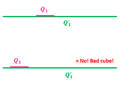
Refer to caption
(a) Separated cubes
Refer to caption
(b) Nested cubes
Refer to caption
(c) Adjacent cubes
Figure 4.1: Relative positions of separated, nested and adjacent cubes.

We preform a similar splitting in the summation ℓ⁡(Q2)≤ℓ⁡(Q2′)\ell(Q_{2})\leq\ell(Q^{\prime}_{2}). Thus, the whole summation is split into nine cases as shown in Table 4.2 below. We explicitly deal with the following six cases. Each of the remaining three cases is symmetric to one of these.

Table 4.2: Splitting of cubes.
(Q1,Q1′)\(Q2,Q2′)(Q_{1},Q^{\prime}_{1})\backslash(Q_{2},Q^{\prime}_{2})      separated      adjacent      nested
separated      case 1      case 2      case 3
adjacent      case 4      case 5
nested      case 6

5 Separated Cubes

In this section, we deal with the cases involving separated cubes. In Section 5.1, we consider the Sep/Sep case when Q1,Q1′Q_{1},Q^{\prime}_{1} are separated and Q2,Q2′Q_{2},Q^{\prime}_{2} are separated. In Section 5.2 we consider the Sep/Nes case when Q1,Q1′Q_{1},Q^{\prime}_{1} are separated and Q2,Q2′Q_{2},Q^{\prime}_{2} are nested. In Section 5.3 we consider the Sep/Adj case when Q1,Q1′Q_{1},Q^{\prime}_{1} are separated and Q2,Q2′Q_{2},Q^{\prime}_{2} are adjacent.

5.1 Separated/Separated cubes

In this section, we consider the Sep/Sep case when Q1,Q1′Q_{1},Q^{\prime}_{1} are separated and Q2,Q2′Q_{2},Q^{\prime}_{2} are separated. That is,

ℓ(Q1)≤ℓ(Q1′),ρ1(Q1,Q1′)>𝒞ℓ(Q1)γ1ℓ(Q1′)1−γ1,and\displaystyle\ell(Q_{1})\leq\ell(Q^{\prime}_{1}),\quad\rho_{1}(Q_{1},Q^{\prime}_{1})>\mathcal{C}\ell(Q_{1})^{\gamma_{1}}\ell(Q^{\prime}_{1})^{1-\gamma_{1}},\quad\text{and}
ℓ⁡(Q2)≤ℓ⁡(Q2′),ρ2​(Q2,Q2′)>𝒞​ℓ​(Q2)γ2​ℓ​(Q2′)1−γ2,\displaystyle\ell(Q_{2})\leq\ell(Q^{\prime}_{2}),\quad\rho_{2}(Q_{2},Q^{\prime}_{2})>\mathcal{C}\ell(Q_{2})^{\gamma_{2}}\ell(Q^{\prime}_{2})^{1-\gamma_{2}},

where 𝒞:=2​A0​CQ​CK\mathcal{C}:=2A_{0}C_{Q}C_{K}.

Recall that we need to estimate (4.7), where |𝔼⁡⟨T​fk,good,gk,good⟩||\mathbb{E}\langle Tf_{k,\text{good}},g_{k,\text{good}}\rangle| can be split into 16 terms. In this Sep/Sep case, the terms involving h0Q1h_{0}^{Q_{1}} or h0Q2h_{0}^{Q_{2}} will disappear. This is because for example, the terms involving h0Q1h_{0}^{Q_{1}} is summed over cubes Q1Q_{1} such that gen​(Q1)=m\text{gen}(Q_{1})=m. This implies δm=ℓ⁡(Q1)≤ℓ⁡(Q1′)≤δm\delta^{m}=\ell(Q_{1})\leq\ell(Q^{\prime}_{1})\leq\delta^{m}, and so ℓ⁡(Q1)=ℓ⁡(Q1′)=δm\ell(Q_{1})=\ell(Q^{\prime}_{1})=\delta^{m}. Thus

ρ1​(Q1,Q1′)>𝒞​ℓ​(Q1)γ1​ℓ​(Q1′)1−γ1≥2​A0​CQ​ℓ​(Q1)≥2​A0​CQ​δm.\rho_{1}(Q_{1},Q^{\prime}_{1})>\mathcal{C}\ell(Q_{1})^{\gamma_{1}}\ell(Q^{\prime}_{1})^{1-\gamma_{1}}\geq 2A_{0}C_{Q}\ell(Q_{1})\geq 2A_{0}C_{Q}\delta^{m}.

This implies Q1∩Rx,m,δ=∅Q_{1}\cap R_{x,m,\delta}=\emptyset or Q1′∩Rx,m,δ=∅Q^{\prime}_{1}\cap R_{x,m,\delta}=\emptyset, where Rx,m,δR_{x,m,\delta} is the support of the functions ff and gg and so

|⟨f,h0Q1⊗hu2Q2⟩|​|⟨g,hu1′Q1′⊗hu2′Q2′⟩|=0.|\langle f,h_{0}^{Q_{1}}\otimes h_{u_{2}}^{Q_{2}}\rangle||\langle g,h_{u^{\prime}_{1}}^{Q^{\prime}_{1}}\otimes h_{u^{\prime}_{2}}^{Q^{\prime}_{2}}\rangle|=0.

Hence, we are left to bound the expression

∑Q1,Q1′separated∑Q2,Q2′separated∑u1,u1′u2,u2′⟨f,hu1Q1⊗hu2Q2⟩​⟨g,hu1′Q1′⊗hu2′Q2′⟩​⟨T⁡(hu1Q1⊗hu2Q2),hu1′Q1′⊗hu2′Q2′⟩\displaystyle\hskip-14.22636pt\sum_{\begin{subarray}{c}Q_{1},Q^{\prime}_{1}\\ \text{separated}\end{subarray}}\,\sum_{\begin{subarray}{c}Q_{2},Q^{\prime}_{2}\\ \text{separated}\end{subarray}}\,\sum_{\begin{subarray}{c}u_{1},u^{\prime}_{1}\\ u_{2},u^{\prime}_{2}\end{subarray}}\,\langle f,h_{u_{1}}^{Q_{1}}\otimes h_{u_{2}}^{Q_{2}}\rangle\langle g,h_{u^{\prime}_{1}}^{Q^{\prime}_{1}}\otimes h_{u^{\prime}_{2}}^{Q^{\prime}_{2}}\rangle\langle T(h_{u_{1}}^{Q_{1}}\otimes h_{u_{2}}^{Q_{2}}),h_{u^{\prime}_{1}}^{Q^{\prime}_{1}}\otimes h_{u^{\prime}_{2}}^{Q^{\prime}_{2}}\rangle
+∑Q1,Q1′separated∑Q2,Q2′ separatedgen​(Q2′)=m∑u1,u1′u2⟨f,hu1Q1⊗hu2Q2⟩⟨g,hu1′Q1′⊗h0Q2′⟩⟨T(hu1Q1⊗hu2Q2),hu1′Q1′⊗h0Q2′⟩\displaystyle+\sum_{\begin{subarray}{c}Q_{1},Q^{\prime}_{1}\\ \text{separated}\end{subarray}}\,\sum_{\begin{subarray}{c}Q_{2},Q^{\prime}_{2}\\ \text{ separated}\\ \text{gen}(Q^{\prime}_{2})=m\end{subarray}}\,\sum_{\begin{subarray}{c}u_{1},u^{\prime}_{1}\\ u_{2}\end{subarray}}\,\langle f,h_{u_{1}}^{Q_{1}}\otimes h_{u_{2}}^{Q_{2}}\rangle\langle g,h_{u^{\prime}_{1}}^{Q^{\prime}_{1}}\otimes h_{0}^{Q^{\prime}_{2}}\rangle\langle T(h_{u_{1}}^{Q_{1}}\otimes h_{u_{2}}^{Q_{2}}),h_{u^{\prime}_{1}}^{Q^{\prime}_{1}}\otimes h_{0}^{Q^{\prime}_{2}}\rangle
+∑Q1,Q1′separatedgen​(Q1′)=m∑Q2,Q2′separated∑u1u2,u2′⟨f,hu1Q1⊗hu2Q2⟩⟨g,h0Q1′⊗hu2′Q2′⟩⟨T(hu1Q1⊗hu2Q2),h0Q1′⊗hu2′Q2′⟩\displaystyle+\sum_{\begin{subarray}{c}Q_{1},Q^{\prime}_{1}\\ \text{separated}\\ \text{gen}(Q^{\prime}_{1})=m\end{subarray}}\,\sum_{\begin{subarray}{c}Q_{2},Q^{\prime}_{2}\\ \text{separated}\end{subarray}}\,\sum_{\begin{subarray}{c}u_{1}\\ u_{2},u^{\prime}_{2}\end{subarray}}\,\langle f,h_{u_{1}}^{Q_{1}}\otimes h_{u_{2}}^{Q_{2}}\rangle\langle g,h_{0}^{Q^{\prime}_{1}}\otimes h_{u^{\prime}_{2}}^{Q^{\prime}_{2}}\rangle\langle T(h_{u_{1}}^{Q_{1}}\otimes h_{u_{2}}^{Q_{2}}),h_{0}^{Q^{\prime}_{1}}\otimes h_{u^{\prime}_{2}}^{Q^{\prime}_{2}}\rangle
+∑Q1,Q1′separatedgen​(Q1′)=m∑Q2,Q2′separatedgen​(Q2′)=m∑u1u2⟨f,hu1Q1⊗hu2Q2⟩⟨g,h0Q1′⊗h0Q2′⟩⟨T(hu1Q1⊗hu2Q2),h0Q1′⊗h0Q2′⟩.\displaystyle+\sum_{\begin{subarray}{c}Q_{1},Q^{\prime}_{1}\\ \text{separated}\\ \text{gen}(Q^{\prime}_{1})=m\end{subarray}}\,\sum_{\begin{subarray}{c}Q_{2},Q^{\prime}_{2}\\ \text{separated}\\ \text{gen}(Q^{\prime}_{2})=m\end{subarray}}\,\sum_{\begin{subarray}{c}u_{1}\\ u_{2}\end{subarray}}\,\langle f,h_{u_{1}}^{Q_{1}}\otimes h_{u_{2}}^{Q_{2}}\rangle\langle g,h_{0}^{Q^{\prime}_{1}}\otimes h_{0}^{Q^{\prime}_{2}}\rangle\langle T(h_{u_{1}}^{Q_{1}}\otimes h_{u_{2}}^{Q_{2}}),h_{0}^{Q^{\prime}_{1}}\otimes h_{0}^{Q^{\prime}_{2}}\rangle. (5.1)

We will estimate the first sum in (5.1). The remaining three sums can be handled analogously. Our proof requires the use of Lemma 5.42, which is also the main result in this section. For i=1,2i=1,2 we define D⁡(Qi,Qi′):=ℓ⁡(Qi)+ℓ⁡(Qi′)+ρi​(Qi,Qi′)D(Q_{i},Q^{\prime}_{i}):=\ell(Q_{i})+\ell(Q^{\prime}_{i})+\rho_{i}(Q_{i},Q^{\prime}_{i}).

Lemma 5.42.

Let Q1∈𝒟1,Q1′∈𝒟1′,Q2∈𝒟2,Q2′∈𝒟2′Q_{1}\in\mathcal{D}_{1},Q^{\prime}_{1}\in\mathcal{D}^{\prime}_{1},Q_{2}\in\mathcal{D}_{2},Q^{\prime}_{2}\in\mathcal{D}^{\prime}_{2} be such that Q1Q_{1} and Q1′Q^{\prime}_{1} are separated and Q2Q_{2} and Q2′Q^{\prime}_{2} are separated. Let fQ1f_{Q_{1}}, fQ1′f_{Q^{\prime}_{1}}, fQ2f_{Q_{2}}, fQ2′f_{Q^{\prime}_{2}} be L2​(μ)L^{2}(\mu) functions supported on cubes Q1Q_{1}, Q1′Q^{\prime}_{1}, Q2Q_{2}, Q2′Q^{\prime}_{2}, respectively. Also assume that

‖fQ1‖L2​(μ1)=‖fQ1′‖L2​(μ1)=‖fQ2‖L2​(μ2)=‖fQ2′‖L2​(μ2)=1\|f_{Q_{1}}\|_{L^{2}(\mu_{1})}=\|f_{Q^{\prime}_{1}}\|_{L^{2}(\mu_{1})}=\|f_{Q_{2}}\|_{L^{2}(\mu_{2})}=\|f_{Q^{\prime}_{2}}\|_{L^{2}(\mu_{2})}=1

and ∫fQ1​d​μ1=∫fQ2​d​μ2=0\int f_{Q_{1}}\,d\mu_{1}=\int f_{Q_{2}}\,d\mu_{2}=0. Then there holds that

|⟨T⁡(fQ1⊗fQ2),gQ1′⊗gQ2′⟩|≲AQ1​Q1′sep​AQ2​Q2′sep,|\langle T(f_{Q_{1}}\otimes f_{Q_{2}}),g_{Q^{\prime}_{1}}\otimes g_{Q^{\prime}_{2}}\rangle|\lesssim A_{Q_{1}Q^{\prime}_{1}}^{\textup{sep}}A_{Q_{2}Q^{\prime}_{2}}^{\textup{sep}},

where

AQ1​Q1′sep:=ℓ​(Q1)α1/2​ℓ​(Q1′)α1/2D​(Q1,Q1′)α1​supz∈Q1λ1​(z,ρ1​(Q1,Q1′))​μ1​(Q1)1/2​μ1​(Q1′)1/2A_{Q_{1}Q^{\prime}_{1}}^{\textup{sep}}:=\frac{\ell(Q_{1})^{\alpha_{1}/2}\ell(Q^{\prime}_{1})^{\alpha_{1}/2}}{D(Q_{1},Q^{\prime}_{1})^{\alpha_{1}}\sup_{z\in Q_{1}}\lambda_{1}(z,\rho_{1}(Q_{1},Q^{\prime}_{1}))}\mu_{1}(Q_{1})^{1/2}\mu_{1}(Q^{\prime}_{1})^{1/2}

and

AQ2​Q2′sep:=ℓ​(Q2)α2/2​ℓ​(Q2′)α2/2D​(Q2,Q2′)α2​supz∈Q2λ2​(z,ρ2​(Q2,Q2′))​μ2​(Q2)1/2​μ1​(Q2′)1/2.A_{Q_{2}Q^{\prime}_{2}}^{\textup{sep}}:=\frac{\ell(Q_{2})^{\alpha_{2}/2}\ell(Q^{\prime}_{2})^{\alpha_{2}/2}}{D(Q_{2},Q^{\prime}_{2})^{\alpha_{2}}\sup_{z\in Q_{2}}\lambda_{2}(z,\rho_{2}(Q_{2},Q^{\prime}_{2}))}\mu_{2}(Q_{2})^{1/2}\mu_{1}(Q^{\prime}_{2})^{1/2}.
Proof.

Since Q1Q_{1} and Q1′Q^{\prime}_{1} are separated, for y1,z∈Q1y_{1},z\in Q_{1} and x1∈Q1′x_{1}\in Q^{\prime}_{1} we have

ρ1​(y1,z)≤CQ​ℓ​(Q1)≤2​A0​CQ​ℓ​(Q1)γ1​ℓ​(Q1′)1−γ1≤ρ1​(Q1,Q1′)CK≤ρ1​(x1,z)CK.\rho_{1}(y_{1},z)\leq C_{Q}\ell(Q_{1})\leq 2A_{0}C_{Q}\ell(Q_{1})^{\gamma_{1}}\ell(Q^{\prime}_{1})^{1-\gamma_{1}}\leq\frac{\rho_{1}(Q_{1},Q^{\prime}_{1})}{C_{K}}\leq\frac{\rho_{1}(x_{1},z)}{C_{K}}. (5.2)

Similarly, for y2,w∈Q2y_{2},w\in Q_{2} and x2∈Q2′x_{2}\in Q^{\prime}_{2} we have

ρ2​(y2,w)≤ρ2​(x2,w)CK.\rho_{2}(y_{2},w)\leq\frac{\rho_{2}(x_{2},w)}{C_{K}}.

Applying Lemma 2.12 to ϕ1=fQ1\phi_{1}=f_{Q_{1}}, ϕ2=fQ2\phi_{2}=f_{Q_{2}}, θ1=gQ1′\theta_{1}=g_{Q^{\prime}_{1}} and θ2=gQ2′\theta_{2}=g_{Q^{\prime}_{2}} we have

|⟨T⁡(fQ1⊗fQ2),gQ1′⊗gQ2′⟩|\displaystyle|\langle T(f_{Q_{1}}\otimes f_{Q_{2}}),g_{Q^{\prime}_{1}}\otimes g_{Q^{\prime}_{2}}\rangle| ≲\displaystyle\lesssim ‖fQ1‖L2​(μ1)​‖fQ2‖L2​(μ2)​μ1​(Q1)1/2​μ2​(Q2)1/2\displaystyle\|f_{Q_{1}}\|_{L^{2}(\mu_{1})}\|f_{Q_{2}}\|_{L^{2}(\mu_{2})}\mu_{1}(Q_{1})^{1/2}\mu_{2}(Q_{2})^{1/2} (5.3)
×∫Q1′CQα1​ℓ​(Q1)α1ρ1​(x1,z)α1​λ1​(z,ρ1​(x1,z))​|gQ1′​(x1)|​d​μ1​(x1)\displaystyle\times\int_{Q^{\prime}_{1}}\frac{C_{Q}^{\alpha_{1}}\ell(Q_{1})^{\alpha_{1}}}{\rho_{1}(x_{1},z)^{\alpha_{1}}\lambda_{1}(z,\rho_{1}(x_{1},z))}|g_{Q^{\prime}_{1}}(x_{1})|\,d\mu_{1}(x_{1})
×∫Q2′CQα2​ℓ​(Q2)α2ρ2​(x2,w)α2​λ2​(w,ρ2​(x2,w))​|gQ2′​(x2)|​d​μ2​(x2).\displaystyle\times\int_{Q^{\prime}_{2}}\frac{C_{Q}^{\alpha_{2}}\ell(Q_{2})^{\alpha_{2}}}{\rho_{2}(x_{2},w)^{\alpha_{2}}\lambda_{2}(w,\rho_{2}(x_{2},w))}|g_{Q^{\prime}_{2}}(x_{2})|\,d\mu_{2}(x_{2}).

Lemma 5.43 below will be used to estimate the two integrals above.

Lemma 5.43.

Let Q1∈𝒟1,Q1′∈𝒟1′,Q2∈𝒟2,Q2′∈𝒟2′Q_{1}\in\mathcal{D}_{1},Q^{\prime}_{1}\in\mathcal{D}^{\prime}_{1},Q_{2}\in\mathcal{D}_{2},Q^{\prime}_{2}\in\mathcal{D}^{\prime}_{2} be such that Q1Q_{1} and Q1′Q^{\prime}_{1} are separated and Q2Q_{2} and Q2′Q^{\prime}_{2} are separated. Suppose z∈Q1z\in Q_{1} and w∈Q2w\in Q_{2}. Then the following hold

ℓ​(Q1)α1ρ1​(Q1,Q1′)α1​λ1​(z,ρ1​(Q1,Q1′))≲ℓ​(Q1)α1/2​ℓ​(Q1′)α1/2D​(Q1,Q1′)α1​λ1​(z,D⁡(Q1,Q1′)),\frac{\ell(Q_{1})^{\alpha_{1}}}{\rho_{1}(Q_{1},Q^{\prime}_{1})^{\alpha_{1}}\lambda_{1}(z,\rho_{1}(Q_{1},Q^{\prime}_{1}))}\lesssim\frac{\ell(Q_{1})^{\alpha_{1}/2}\ell(Q^{\prime}_{1})^{\alpha_{1}/2}}{D(Q_{1},Q^{\prime}_{1})^{\alpha_{1}}\lambda_{1}(z,D(Q_{1},Q^{\prime}_{1}))}, (5.4)

and

ℓ​(Q2)α2ρ2​(Q2,Q2′)α2​λ2​(w,ρ2​(Q2,Q2′))≲ℓ​(Q2)α2/2​ℓ​(Q2′)α2/2D​(Q2,Q2′)α2​λ2​(w,D⁡(Q2,Q2′)).\frac{\ell(Q_{2})^{\alpha_{2}}}{\rho_{2}(Q_{2},Q^{\prime}_{2})^{\alpha_{2}}\lambda_{2}(w,\rho_{2}(Q_{2},Q^{\prime}_{2}))}\lesssim\frac{\ell(Q_{2})^{\alpha_{2}/2}\ell(Q^{\prime}_{2})^{\alpha_{2}/2}}{D(Q_{2},Q^{\prime}_{2})^{\alpha_{2}}\lambda_{2}(w,D(Q_{2},Q^{\prime}_{2}))}. (5.5)

Proof of Lemma 5.43. Consider the case ρ1​(Q1,Q1′)≥ℓ⁡(Q1′)\rho_{1}(Q_{1},Q^{\prime}_{1})\geq\ell(Q^{\prime}_{1}), where we have

D⁡(Q1,Q1′)\displaystyle D(Q_{1},Q^{\prime}_{1}) =\displaystyle= ℓ⁡(Q1)+ℓ⁡(Q1′)+ρ1​(Q1,Q1′)≤ℓ⁡(Q1)+ρ1​(Q1,Q1′)+ρ1​(Q1,Q1′)\displaystyle\ell(Q_{1})+\ell(Q^{\prime}_{1})+\rho_{1}(Q_{1},Q^{\prime}_{1})\leq\ell(Q_{1})+\rho_{1}(Q_{1},Q^{\prime}_{1})+\rho_{1}(Q_{1},Q^{\prime}_{1})
≤\displaystyle\leq ℓ⁡(Q1′)+2​ρ1​(Q1,Q1′)≤3​ρ1​(Q1,Q1′).\displaystyle\ell(Q^{\prime}_{1})+2\rho_{1}(Q_{1},Q^{\prime}_{1})\leq 3\rho_{1}(Q_{1},Q^{\prime}_{1}).

Since λ1\lambda_{1} is non-decreasing with respect to its second variable and is doubling,

λ1​(z,ρ1​(Q1,Q1′))≥λ1​(z,D⁡(Q1,Q1′)3)≥Cλ1−(log2⁡3+1)​λ1​(z,D⁡(Q1,Q1′)).\lambda_{1}(z,\rho_{1}(Q_{1},Q^{\prime}_{1}))\geq\lambda_{1}\bigg(z,\frac{D(Q_{1},Q^{\prime}_{1})}{3}\bigg)\geq C_{\lambda_{1}}^{-(\log_{2}3+1)}\lambda_{1}(z,D(Q_{1},Q^{\prime}_{1})).

Hence when ρ1​(Q1,Q1′)≥ℓ⁡(Q1′)\rho_{1}(Q_{1},Q^{\prime}_{1})\geq\ell(Q^{\prime}_{1}) we have

ℓ​(Q1)α1ρ1​(Q1,Q1′)α1​λ1​(z,ρ1​(Q1,Q1′))≲ℓ​(Q1)α1/2​ℓ​(Q1′)α1/2D​(Q1,Q1′)α1​λ1​(z,D⁡(Q1,Q1′)).\frac{\ell(Q_{1})^{\alpha_{1}}}{\rho_{1}(Q_{1},Q^{\prime}_{1})^{\alpha_{1}}\lambda_{1}(z,\rho_{1}(Q_{1},Q^{\prime}_{1}))}\lesssim\frac{\ell(Q_{1})^{\alpha_{1}/2}\ell(Q^{\prime}_{1})^{\alpha_{1}/2}}{D(Q_{1},Q^{\prime}_{1})^{\alpha_{1}}\lambda_{1}(z,D(Q_{1},Q^{\prime}_{1}))}. (5.6)

Consider the case ρ1​(Q1,Q1′)<ℓ⁡(Q1′)\rho_{1}(Q_{1},Q^{\prime}_{1})<\ell(Q^{\prime}_{1}). Here

D⁡(Q1,Q1′)=ℓ⁡(Q1)+ℓ⁡(Q1′)+ρ1​(Q1,Q1′)<ℓ⁡(Q1′)+ℓ⁡(Q1′)+ℓ⁡(Q1′)=3​ℓ​(Q1′).D(Q_{1},Q^{\prime}_{1})=\ell(Q_{1})+\ell(Q^{\prime}_{1})+\rho_{1}(Q_{1},Q^{\prime}_{1})<\ell(Q^{\prime}_{1})+\ell(Q^{\prime}_{1})+\ell(Q^{\prime}_{1})=3\ell(Q^{\prime}_{1}).

Again, since λ1\lambda_{1} is non-decreasing and is doubling,

λ1​(z,ρ1​(Q1,Q1′))\displaystyle\lambda_{1}(z,\rho_{1}(Q_{1},Q^{\prime}_{1})) >\displaystyle> λ1​(z,𝒞​ℓ​(Q1)γ1​ℓ​(Q1′)1−γ1)>λ1​(z,ℓ​(Q1)γ1​ℓ​(Q1′)1−γ1)\displaystyle\lambda_{1}(z,\mathcal{C}\ell(Q_{1})^{\gamma_{1}}\ell(Q^{\prime}_{1})^{1-\gamma_{1}})>\lambda_{1}(z,\ell(Q_{1})^{\gamma_{1}}\ell(Q^{\prime}_{1})^{1-\gamma_{1}})
≳\displaystyle\gtrsim Cλ1OPEN−γ1​log2​ℓ⁡(Q1′CLOSEℓ⁡(Q1))​λ1​(z,ℓ⁡(Q1′))=(ℓ⁡(Q1)ℓ⁡(Q1′))t1​γ1​λ1​(z,ℓ⁡(Q1′)).\displaystyle C_{\lambda_{1}}^{-\gamma_{1}\log_{2}\frac{\ell(Q^{\prime}_{1}}{\ell(Q_{1})})}\lambda_{1}(z,\ell(Q^{\prime}_{1}))=\bigg(\frac{\ell(Q_{1})}{\ell(Q^{\prime}_{1})}\bigg)^{t_{1}\gamma_{1}}\lambda_{1}(z,\ell(Q^{\prime}_{1})).

The last equality above is due to the facts that Cλ1≥1C_{\lambda_{1}}\geq 1 and t1:=log2⁡Cλ1t_{1}:=\log_{2}C_{\lambda_{1}}, which imply

Cλ1−γ1​log2​ℓ⁡(Q1′)ℓ⁡(Q1)=2−t1​γ1​log2​ℓ⁡(Q1′)ℓ⁡(Q1)=(ℓ⁡(Q1)ℓ⁡(Q1′))t1​γ1.C_{\lambda_{1}}^{-\gamma_{1}\log_{2}\frac{\ell(Q^{\prime}_{1})}{\ell(Q_{1})}}=2^{-t_{1}\gamma_{1}\log_{2}\frac{\ell(Q^{\prime}_{1})}{\ell(Q_{1})}}=\bigg(\frac{\ell(Q_{1})}{\ell(Q^{\prime}_{1})}\bigg)^{t_{1}\gamma_{1}}.

Combining with the fact that α1​γ1+t1​γ1=α1/2\alpha_{1}\gamma_{1}+t_{1}\gamma_{1}=\alpha_{1}/2 we have

ℓ​(Q1)α1ρ1​(Q1,Q1′)α1​λ1​(z,ρ1​(Q1,Q1′))\displaystyle\frac{\ell(Q_{1})^{\alpha_{1}}}{\rho_{1}(Q_{1},Q^{\prime}_{1})^{\alpha_{1}}\lambda_{1}(z,\rho_{1}(Q_{1},Q^{\prime}_{1}))} ≲\displaystyle\lesssim ℓ​(Q1)α1𝒞α1​ℓ​(Q1)α1​γ1​ℓ​(Q1′)(1−γ1)​α1​ℓ​(Q1)t1​γ1​ℓ​(Q1′)−t1​γ1​λ1​(z,ℓ⁡(Q1′))\displaystyle\frac{\ell(Q_{1})^{\alpha_{1}}}{\mathcal{C}^{\alpha_{1}}\ell(Q_{1})^{\alpha_{1}\gamma_{1}}\ell(Q^{\prime}_{1})^{(1-\gamma_{1})\alpha_{1}}\ell(Q_{1})^{t_{1}\gamma_{1}}\ell(Q^{\prime}_{1})^{-t_{1}\gamma_{1}}\lambda_{1}(z,\ell(Q^{\prime}_{1}))} (5.7)
=\displaystyle= ℓ​(Q1)α1−(α1​γ1+t1​γ1)​ℓ​(Q1′)α1​γ1+t1​γ1𝒞α1​ℓ​(Q1′)α1​λ1​(z,ℓ⁡(Q1′))\displaystyle\frac{\ell(Q_{1})^{\alpha_{1}-(\alpha_{1}\gamma_{1}+t_{1}\gamma_{1})}\ell(Q^{\prime}_{1})^{\alpha_{1}\gamma_{1}+t_{1}\gamma_{1}}}{\mathcal{C}^{\alpha_{1}}\ell(Q^{\prime}_{1})^{\alpha_{1}}\lambda_{1}(z,\ell(Q^{\prime}_{1}))}
=\displaystyle= ℓ​(Q1)α1/2​ℓ​(Q1′)α1/2𝒞α1​ℓ​(Q1′)α1​λ1​(z,ℓ⁡(Q1′))\displaystyle\frac{\ell(Q_{1})^{\alpha_{1}/2}\ell(Q^{\prime}_{1})^{\alpha_{1}/2}}{\mathcal{C}^{\alpha_{1}}\ell(Q^{\prime}_{1})^{\alpha_{1}}\lambda_{1}(z,\ell(Q^{\prime}_{1}))}
≲\displaystyle\lesssim ℓ​(Q1)α1/2​ℓ​(Q1′)α1/2D​(Q1,Q1′)α1​λ1​(z,D⁡(Q1,Q1′)).\displaystyle\frac{\ell(Q_{1})^{\alpha_{1}/2}\ell(Q^{\prime}_{1})^{\alpha_{1}/2}}{D(Q_{1},Q^{\prime}_{1})^{\alpha_{1}}\lambda_{1}(z,D(Q_{1},Q^{\prime}_{1}))}.

From (5.6) and (5.7), in both cases we have

ℓ​(Q1)α1ρ1​(Q1,Q1′)α1​λ1​(z,ρ1​(Q1,Q1′))≲ℓ​(Q1)α1/2​ℓ​(Q1′)α1/2D​(Q1,Q1′)α1​λ1​(z,D⁡(Q1,Q1′)).\frac{\ell(Q_{1})^{\alpha_{1}}}{\rho_{1}(Q_{1},Q^{\prime}_{1})^{\alpha_{1}}\lambda_{1}(z,\rho_{1}(Q_{1},Q^{\prime}_{1}))}\lesssim\frac{\ell(Q_{1})^{\alpha_{1}/2}\ell(Q^{\prime}_{1})^{\alpha_{1}/2}}{D(Q_{1},Q^{\prime}_{1})^{\alpha_{1}}\lambda_{1}(z,D(Q_{1},Q^{\prime}_{1}))}.

Following the same procedure we also obtain

ℓ​(Q2)α2ρ2​(Q2,Q2′)α2​λ2​(w,ρ2​(Q2,Q2′))≲ℓ​(Q2)α2/2​ℓ​(Q2′)α2/2D​(Q2,Q2′)α2​λ2​(w,D⁡(Q2,Q2′)).\frac{\ell(Q_{2})^{\alpha_{2}}}{\rho_{2}(Q_{2},Q^{\prime}_{2})^{\alpha_{2}}\lambda_{2}(w,\rho_{2}(Q_{2},Q^{\prime}_{2}))}\lesssim\frac{\ell(Q_{2})^{\alpha_{2}/2}\ell(Q^{\prime}_{2})^{\alpha_{2}/2}}{D(Q_{2},Q^{\prime}_{2})^{\alpha_{2}}\lambda_{2}(w,D(Q_{2},Q^{\prime}_{2}))}.

This completes the proof of Lemma 5.43. □\hfill\Box

Using Lemma 5.43 we have

∫Q1′CQα1​ℓ​(Q1)α1​|gQ1′​(x1)|ρ1​(x1,z)α1​λ1​(z,ρ1​(x1,z))​d​μ1​(x1)≲ℓ​(Q1)α1/2​ℓ​(Q1′)α1/2D​(Q1,Q1′)α1​λ1​(z,D⁡(Q1,Q1′))​μ1​(Q1′)1/2≲AQ1​Q1′sepμ1​(Q1)1/2,\displaystyle\int_{Q^{\prime}_{1}}\frac{C_{Q}^{\alpha_{1}}\ell(Q_{1})^{\alpha_{1}}|g_{Q^{\prime}_{1}}(x_{1})|}{\rho_{1}(x_{1},z)^{\alpha_{1}}\lambda_{1}(z,\rho_{1}(x_{1},z))}\,d\mu_{1}(x_{1})\lesssim\frac{\ell(Q_{1})^{\alpha_{1}/2}\ell(Q^{\prime}_{1})^{\alpha_{1}/2}}{D(Q_{1},Q^{\prime}_{1})^{\alpha_{1}}\lambda_{1}(z,D(Q_{1},Q^{\prime}_{1}))}\mu_{1}(Q^{\prime}_{1})^{1/2}\lesssim\frac{A_{Q_{1}Q^{\prime}_{1}}^{\textup{sep}}}{\mu_{1}(Q_{1})^{1/2}},

and

∫Q2′CQα2​ℓ​(Q2)α2​|gQ2′​(x2)|ρ2​(x2,w)α2​λ2​(w,ρ2​(x2,w))​d​μ2​(x2)≲ℓ​(Q2)α2/2​ℓ​(Q2′)α2/2D​(Q2,Q2′)α2​λ2​(w,D⁡(Q2,Q2′))​μ2​(Q2′)1/2≲AQ2​Q2′sepμ2​(Q2)1/2.\displaystyle\int_{Q^{\prime}_{2}}\frac{C_{Q}^{\alpha_{2}}\ell(Q_{2})^{\alpha_{2}}|g_{Q^{\prime}_{2}}(x_{2})|}{\rho_{2}(x_{2},w)^{\alpha_{2}}\lambda_{2}(w,\rho_{2}(x_{2},w))}\,d\mu_{2}(x_{2})\lesssim\frac{\ell(Q_{2})^{\alpha_{2}/2}\ell(Q^{\prime}_{2})^{\alpha_{2}/2}}{D(Q_{2},Q^{\prime}_{2})^{\alpha_{2}}\lambda_{2}(w,D(Q_{2},Q^{\prime}_{2}))}\mu_{2}(Q^{\prime}_{2})^{1/2}\lesssim\frac{A_{Q_{2}Q^{\prime}_{2}}^{\textup{sep}}}{\mu_{2}(Q_{2})^{1/2}}.

Thus, (5.3) becomes

|⟨T⁡(fQ1⊗fQ2,gQ1′⊗gQ2′)⟩|≲AQ1​Q1′sep​AQ2​Q2′sep,|\langle T(f_{Q_{1}}\otimes f_{Q_{2}},g_{Q^{\prime}_{1}}\otimes g_{Q^{\prime}_{2}})\rangle|\lesssim A_{Q_{1}Q^{\prime}_{1}}^{\textup{sep}}A_{Q_{2}Q^{\prime}_{2}}^{\textup{sep}},

as required. ∎

The following proposition estimates the sum involving AQ1​Q1′sepA_{Q_{1}Q^{\prime}_{1}}^{\textup{sep}}.

Proposition 5.44.

For each Q1∈𝒟1Q_{1}\in\mathcal{D}_{1} and Q1′∈𝒟1′Q^{\prime}_{1}\in\mathcal{D}^{\prime}_{1}, given nonnegative constants aQ1,bQ1′≥0a_{Q_{1}},b_{Q^{\prime}_{1}}\geq 0, we have

∑Q1,Q1′separatedAQ1,Q1′sep​aQ1​bQ1′≲(∑Q1aQ12)1/2​(∑Q1′bQ1′2)1/2.\sum_{\begin{subarray}{c}Q_{1},Q^{\prime}_{1}\\ \textup{separated}\end{subarray}}A_{Q_{1},Q^{\prime}_{1}}^{\textup{sep}}a_{Q_{1}}b_{Q^{\prime}_{1}}\lesssim\bigg(\sum_{Q_{1}}a_{Q_{1}}^{2}\bigg)^{1/2}\bigg(\sum_{Q^{\prime}_{1}}b_{Q^{\prime}_{1}}^{2}\bigg)^{1/2}.

In fact,

(∑Q1′[∑Q1:ℓ⁡(Q1)≤ℓ⁡(Q1′)AQ1,Q1′sepaQ1]2)1/2≲(∑Q1aQ12)1/2.\left(\sum_{Q^{\prime}_{1}}\left[\sum_{Q_{1}:\ell(Q_{1})\leq\ell(Q^{\prime}_{1})}A_{Q_{1},Q^{\prime}_{1}}^{\textup{sep}}a_{Q_{1}}\right]^{2}\right)^{1/2}\lesssim\bigg(\sum_{Q_{1}}a_{Q_{1}}^{2}\bigg)^{1/2}.
Proof.

The proof of Proposition 5.44 is a generalisation of Proposition 6.3 in [22] from non-homogeneous metric spaces to non-homogeneous quasimetric spaces. The proof given there goes through unchanged, as it does not depend on the quasitriangle inequality of quasimetric ρ1\rho_{1}.

There is also an analogue of Proposition 5.44 in non-homogeneous Euclidean spaces stated as Theorem 6.5 in [31]. ∎

Now, applying Lemma 5.42 to fQ1=hu1Q1f_{Q_{1}}=h_{u_{1}}^{Q_{1}}, fQ2=hu2Q2f_{Q_{2}}=h_{u_{2}}^{Q_{2}}, fQ1′=hu1′Q1′f_{Q^{\prime}_{1}}=h_{u^{\prime}_{1}}^{Q^{\prime}_{1}}, fQ2′=hu2′Q2′f_{Q^{\prime}_{2}}=h_{u^{\prime}_{2}}^{Q^{\prime}_{2}}, and using Proposition 5.44, the first sum in (5.1) is bounded by

∑ℓ⁡(Q1)≤ℓ⁡(Q1′)∑ℓ⁡(Q2)≤ℓ⁡(Q2′)∑u1,u1′u2,u2′AQ1,Q1′sep​AQ2,Q2′sep​|⟨f,hu1Q1⊗hu2Q2⟩|​|⟨g,hu1′Q1′⊗hu2′Q2′⟩|\displaystyle\sum_{\ell(Q_{1})\leq\ell(Q^{\prime}_{1})}\sum_{\ell(Q_{2})\leq\ell(Q^{\prime}_{2})}\sum_{\begin{subarray}{c}u_{1},u^{\prime}_{1}\\ u_{2},u^{\prime}_{2}\end{subarray}}A_{Q_{1},Q^{\prime}_{1}}^{\text{sep}}A_{Q_{2},Q^{\prime}_{2}}^{\text{sep}}|\langle f,h_{u_{1}}^{Q_{1}}\otimes h_{u_{2}}^{Q_{2}}\rangle||\langle g,h_{u^{\prime}_{1}}^{Q^{\prime}_{1}}\otimes h_{u^{\prime}_{2}}^{Q^{\prime}_{2}}\rangle|
≲\displaystyle\lesssim ∑ℓ⁡(Q1)≤ℓ⁡(Q1′)∑u1,u1′AQ1,Q1′sep​(∑Q2∑u2|⟨f,hu1Q1⊗hu2Q2⟩|2)1/2​(∑Q2′∑u2′|⟨g,hu1′Q1′⊗hu2′Q2′⟩|2)1/2\displaystyle\sum_{\ell(Q_{1})\leq\ell(Q^{\prime}_{1})}\sum_{u_{1},u^{\prime}_{1}}A_{Q_{1},Q^{\prime}_{1}}^{\text{sep}}\Big(\sum_{Q_{2}}\sum_{u_{2}}|\langle f,h_{u_{1}}^{Q_{1}}\otimes h_{u_{2}}^{Q_{2}}\rangle|^{2}\Big)^{1/2}\Big(\sum_{Q^{\prime}_{2}}\sum_{u^{\prime}_{2}}|\langle g,h_{u^{\prime}_{1}}^{Q^{\prime}_{1}}\otimes h_{u^{\prime}_{2}}^{Q^{\prime}_{2}}\rangle|^{2}\Big)^{1/2}
≲\displaystyle\lesssim (∑Q1∑u1∑Q2∑u2|⟨f,hu1Q1⊗hu2Q2⟩|2)1/2​(∑Q1′∑u1′∑Q2′∑u2′|⟨g,hu1′Q1′⊗hu2′Q2′⟩|2)1/2\displaystyle\Big(\sum_{Q_{1}}\sum_{u_{1}}\sum_{Q_{2}}\sum_{u_{2}}|\langle f,h_{u_{1}}^{Q_{1}}\otimes h_{u_{2}}^{Q_{2}}\rangle|^{2}\Big)^{1/2}\Big(\sum_{Q^{\prime}_{1}}\sum_{u^{\prime}_{1}}\sum_{Q^{\prime}_{2}}\sum_{u^{\prime}_{2}}|\langle g,h_{u^{\prime}_{1}}^{Q^{\prime}_{1}}\otimes h_{u^{\prime}_{2}}^{Q^{\prime}_{2}}\rangle|^{2}\Big)^{1/2}
≲\displaystyle\lesssim ‖f‖L2​(μ)​‖g‖L2​(μ).\displaystyle\|f\|_{L^{2}(\mu)}\|g\|_{L^{2}(\mu)}.

Similarly, we obtain the same result for other sums in (5.1). This completes the Sep/Sep case.

5.2 Separated/Nested cubes

In this section, we consider the Sep/Nes case. That is, we estimate (4.7) when Q1,Q1′Q_{1},Q^{\prime}_{1} are separated and Q2,Q2′Q_{2},Q^{\prime}_{2} are nested:

ℓ(Q1)≤ℓ(Q1′),ρ1(Q1,Q1′)>𝒞ℓ(Q1)γ1ℓ(Q1′)1−γ1,and\displaystyle\ell(Q_{1})\leq\ell(Q^{\prime}_{1}),\quad\rho_{1}(Q_{1},Q^{\prime}_{1})>\mathcal{C}\ell(Q_{1})^{\gamma_{1}}\ell(Q^{\prime}_{1})^{1-\gamma_{1}},\quad\text{and}
ℓ⁡(Q2)<δr​ℓ​(Q2′),ρ2​(Q2,Q2′)≤𝒞​ℓ​(Q2)γ2​ℓ​(Q2′)1−γ2,\displaystyle\ell(Q_{2})<\delta^{r}\ell(Q^{\prime}_{2}),\quad\rho_{2}(Q_{2},Q^{\prime}_{2})\leq\mathcal{C}\ell(Q_{2})^{\gamma_{2}}\ell(Q^{\prime}_{2})^{1-\gamma_{2}},

where 𝒞:=2​A0​CQ​CK\mathcal{C}:=2A_{0}C_{Q}C_{K}. With the same reason as in the Sep/Sep case, the terms in (4.7) which involves h0Q1h_{0}^{Q_{1}} vanish. Furthermore, the terms involving h0Q2h_{0}^{Q_{2}} also vanish. This is because ℓ⁡(Q2)=δm\ell(Q_{2})=\delta^{m} implies that δ−r​ℓ​(Q2)=δm−r<ℓ⁡(Q2′)≤δm\delta^{-r}\ell(Q_{2})=\delta^{m-r}<\ell(Q^{\prime}_{2})\leq\delta^{m}, which is impossible.

We are left to bound

∑Q1,Q1′separated∑Q2,Q2′nested∑u1,u1′u2,u2′⟨f,hu1Q1⊗hu2Q2⟩​⟨g,hu1′Q1′⊗hu2′Q2′⟩​⟨T⁡(hu1Q1⊗hu2Q2),hu1′Q1′⊗hu2′Q2′⟩\displaystyle\hskip-14.22636pt\sum_{\begin{subarray}{c}Q_{1},Q^{\prime}_{1}\\ \text{separated}\end{subarray}}\,\sum_{\begin{subarray}{c}Q_{2},Q^{\prime}_{2}\\ \text{nested}\end{subarray}}\,\sum_{\begin{subarray}{c}u_{1},u^{\prime}_{1}\\ u_{2},u^{\prime}_{2}\end{subarray}}\,\langle f,h_{u_{1}}^{Q_{1}}\otimes h_{u_{2}}^{Q_{2}}\rangle\langle g,h_{u^{\prime}_{1}}^{Q^{\prime}_{1}}\otimes h_{u^{\prime}_{2}}^{Q^{\prime}_{2}}\rangle\langle T(h_{u_{1}}^{Q_{1}}\otimes h_{u_{2}}^{Q_{2}}),h_{u^{\prime}_{1}}^{Q^{\prime}_{1}}\otimes h_{u^{\prime}_{2}}^{Q^{\prime}_{2}}\rangle
+∑Q1,Q1′separated∑Q2,Q2′ nestedgen​(Q2′)=m∑u1,u1′u2⟨f,hu1Q1⊗hu2Q2⟩⟨g,hu1′Q1′⊗h0Q2′⟩⟨T(hu1Q1⊗hu2Q2),hu1′Q1′⊗h0Q2′⟩\displaystyle+\sum_{\begin{subarray}{c}Q_{1},Q^{\prime}_{1}\\ \text{separated}\end{subarray}}\,\sum_{\begin{subarray}{c}Q_{2},Q^{\prime}_{2}\\ \text{ nested}\\ \text{gen}(Q^{\prime}_{2})=m\end{subarray}}\,\sum_{\begin{subarray}{c}u_{1},u^{\prime}_{1}\\ u_{2}\end{subarray}}\,\langle f,h_{u_{1}}^{Q_{1}}\otimes h_{u_{2}}^{Q_{2}}\rangle\langle g,h_{u^{\prime}_{1}}^{Q^{\prime}_{1}}\otimes h_{0}^{Q^{\prime}_{2}}\rangle\langle T(h_{u_{1}}^{Q_{1}}\otimes h_{u_{2}}^{Q_{2}}),h_{u^{\prime}_{1}}^{Q^{\prime}_{1}}\otimes h_{0}^{Q^{\prime}_{2}}\rangle
+∑Q1,Q1′separatedgen​(Q1′)=m∑Q2,Q2′nested∑u1u2,u2′⟨f,hu1Q1⊗hu2Q2⟩⟨g,h0Q1′⊗hu2′Q2′⟩⟨T(hu1Q1⊗hu2Q2),h0Q1′⊗hu2′Q2′⟩\displaystyle+\sum_{\begin{subarray}{c}Q_{1},Q^{\prime}_{1}\\ \text{separated}\\ \text{gen}(Q^{\prime}_{1})=m\end{subarray}}\,\sum_{\begin{subarray}{c}Q_{2},Q^{\prime}_{2}\\ \text{nested}\end{subarray}}\,\sum_{\begin{subarray}{c}u_{1}\\ u_{2},u^{\prime}_{2}\end{subarray}}\,\langle f,h_{u_{1}}^{Q_{1}}\otimes h_{u_{2}}^{Q_{2}}\rangle\langle g,h_{0}^{Q^{\prime}_{1}}\otimes h_{u^{\prime}_{2}}^{Q^{\prime}_{2}}\rangle\langle T(h_{u_{1}}^{Q_{1}}\otimes h_{u_{2}}^{Q_{2}}),h_{0}^{Q^{\prime}_{1}}\otimes h_{u^{\prime}_{2}}^{Q^{\prime}_{2}}\rangle
+∑Q1,Q1′separatedgen​(Q1′)=m∑Q2,Q2′nestedgen​(Q2′)=m∑u1u2⟨f,hu1Q1⊗hu2Q2⟩⟨g,h0Q1′⊗h0Q2′⟩⟨T(hu1Q1⊗hu2Q2),h0Q1′⊗h0Q2′⟩.\displaystyle+\sum_{\begin{subarray}{c}Q_{1},Q^{\prime}_{1}\\ \text{separated}\\ \text{gen}(Q^{\prime}_{1})=m\end{subarray}}\,\sum_{\begin{subarray}{c}Q_{2},Q^{\prime}_{2}\\ \text{nested}\\ \text{gen}(Q^{\prime}_{2})=m\end{subarray}}\,\sum_{\begin{subarray}{c}u_{1}\\ u_{2}\end{subarray}}\,\langle f,h_{u_{1}}^{Q_{1}}\otimes h_{u_{2}}^{Q_{2}}\rangle\langle g,h_{0}^{Q^{\prime}_{1}}\otimes h_{0}^{Q^{\prime}_{2}}\rangle\langle T(h_{u_{1}}^{Q_{1}}\otimes h_{u_{2}}^{Q_{2}}),h_{0}^{Q^{\prime}_{1}}\otimes h_{0}^{Q^{\prime}_{2}}\rangle. (5.8)

We will handle the first two terms in (5.2). The last two terms can be estimated analogously. We write ⟨T⁡(hu1Q1⊗hu2Q2),hu1′Q1′⊗hu2′Q2′⟩\langle T(h_{u_{1}}^{Q_{1}}\otimes h_{u_{2}}^{Q_{2}}),h_{u^{\prime}_{1}}^{Q^{\prime}_{1}}\otimes h_{u^{\prime}_{2}}^{Q^{\prime}_{2}}\rangle as the sum

(⟨T⁡(hu1Q1⊗hu2Q2),hu1′Q1′⊗hu2′Q2′⟩−⟨hu2′Q2′⟩Q2​⟨T⁡(hu1Q1⊗hu2Q2),hy1′Q1′⊗1⟩)\displaystyle(\langle T(h_{u_{1}}^{Q_{1}}\otimes h_{u_{2}}^{Q_{2}}),h_{u^{\prime}_{1}}^{Q^{\prime}_{1}}\otimes h_{u^{\prime}_{2}}^{Q^{\prime}_{2}}\rangle-\langle h_{u^{\prime}_{2}}^{Q^{\prime}_{2}}\rangle_{Q_{2}}\langle T(h_{u_{1}}^{Q_{1}}\otimes h_{u_{2}}^{Q_{2}}),h_{y^{\prime}_{1}}^{Q^{\prime}_{1}}\otimes 1\rangle)
+⟨hu2′Q2′⟩Q2​⟨T⁡(hu1Q1⊗hu2Q2),hu1′Q1′⊗1⟩.\displaystyle\qquad+\,\langle h_{u^{\prime}_{2}}^{Q^{\prime}_{2}}\rangle_{Q_{2}}\langle T(h_{u_{1}}^{Q_{1}}\otimes h_{u_{2}}^{Q_{2}}),h_{u^{\prime}_{1}}^{Q^{\prime}_{1}}\otimes 1\rangle.

Here ⟨h⟩Q:=μ2​(Q)−1​∫Qh​d​μ2\langle h\rangle_{Q}:=\mu_{2}(Q)^{-1}\int_{Q}h\,d\mu_{2}. Let Q2,1′∈ch​(Q2′)Q^{\prime}_{2,1}\in\text{ch}(Q^{\prime}_{2}) be the child of Q2′Q^{\prime}_{2} such that Q2⊂Q2,1′Q_{2}\subset Q^{\prime}_{2,1}. As noted in Section 4.2, there is such a child Q2,1′Q^{\prime}_{2,1} because Q2Q_{2} and Q2′Q^{\prime}_{2} are nested and Q2Q_{2} is good. Since Q2⊂Q2,1′Q_{2}\subset Q^{\prime}_{2,1}, and hu2′Q2′h_{u^{\prime}_{2}}^{Q^{\prime}_{2}} is constant on Q2,1′Q^{\prime}_{2,1}, we have

⟨hu2′Q2′⟩Q2=⟨hu2′Q2′⟩Q2,1′=C.\langle h_{u^{\prime}_{2}}^{Q^{\prime}_{2}}\rangle_{Q_{2}}=\langle h_{u^{\prime}_{2}}^{Q^{\prime}_{2}}\rangle_{Q^{\prime}_{2,1}}=C.

We first consider the matrix element

⟨T⁡(hu1Q1⊗hu2Q2),hu1′Q1′⊗hu2′Q2′⟩−⟨hu2′Q2′⟩Q2​⟨T⁡(hu1Q1⊗hu2Q2),hu1′Q1′⊗1⟩\displaystyle\langle T(h_{u_{1}}^{Q_{1}}\otimes h_{u_{2}}^{Q_{2}}),h_{u^{\prime}_{1}}^{Q^{\prime}_{1}}\otimes h_{u^{\prime}_{2}}^{Q^{\prime}_{2}}\rangle-\langle h_{u^{\prime}_{2}}^{Q^{\prime}_{2}}\rangle_{Q_{2}}\langle T(h_{u_{1}}^{Q_{1}}\otimes h_{u_{2}}^{Q_{2}}),h_{u^{\prime}_{1}}^{Q^{\prime}_{1}}\otimes 1\rangle
=\displaystyle= ∑Q′∈ch​(Q2′)Q′⊂Q2′\Q2,1′⟨T⁡(hu1Q1⊗hu2Q2),hu1′Q1′⊗hu2′Q2′​χQ′⟩+⟨T⁡(hu1Q1⊗hu2Q2),hu1′Q1′⊗hu2′Q2′​χQ2,1′⟩\displaystyle\sum_{\begin{subarray}{c}Q^{\prime}\in\text{ch}(Q^{\prime}_{2})\\ Q^{\prime}\subset Q^{\prime}_{2}\backslash Q^{\prime}_{2,1}\end{subarray}}\langle T(h_{u_{1}}^{Q_{1}}\otimes h_{u_{2}}^{Q_{2}}),h_{u^{\prime}_{1}}^{Q^{\prime}_{1}}\otimes h_{u^{\prime}_{2}}^{Q^{\prime}_{2}}\chi_{Q^{\prime}}\rangle+\langle T(h_{u_{1}}^{Q_{1}}\otimes h_{u_{2}}^{Q_{2}}),h_{u^{\prime}_{1}}^{Q^{\prime}_{1}}\otimes h_{u^{\prime}_{2}}^{Q^{\prime}_{2}}\chi_{Q^{\prime}_{2,1}}\rangle
−⟨hu2′Q2′⟩Q2,1′​⟨T⁡(hu1Q1⊗hu2Q2),hu1′Q1′⊗χQ2,1c′⟩−⟨hu2′Q2′⟩Q2,1′​⟨T⁡(hu1Q1⊗hu2Q2),hu1′Q1′⊗χQ2,1′⟩\displaystyle-\langle h_{u^{\prime}_{2}}^{Q^{\prime}_{2}}\rangle_{Q^{\prime}_{2,1}}\langle T(h_{u_{1}}^{Q_{1}}\otimes h_{u_{2}}^{Q_{2}}),h_{u^{\prime}_{1}}^{Q^{\prime}_{1}}\otimes\chi_{Q^{{}^{\prime}c}_{2,1}}\rangle-\langle h_{u^{\prime}_{2}}^{Q^{\prime}_{2}}\rangle_{Q^{\prime}_{2,1}}\langle T(h_{u_{1}}^{Q_{1}}\otimes h_{u_{2}}^{Q_{2}}),h_{u^{\prime}_{1}}^{Q^{\prime}_{1}}\otimes\chi_{Q^{\prime}_{2,1}}\rangle
=\displaystyle= ∑Q′∈ch​(Q2′)Q′⊂Q2′\Q2,1′⟨T⁡(hu1Q1⊗hu2Q2),hu1′Q1′⊗hu2′Q2′​χQ′⟩−⟨hu2′Q2′⟩Q2,1′​⟨T⁡(hu1Q1⊗hu2Q2),hu1′Q1′⊗χQ2,1c′⟩.\displaystyle\sum_{\begin{subarray}{c}Q^{\prime}\in\text{ch}(Q^{\prime}_{2})\\ Q^{\prime}\subset Q^{\prime}_{2}\backslash Q^{\prime}_{2,1}\end{subarray}}\langle T(h_{u_{1}}^{Q_{1}}\otimes h_{u_{2}}^{Q_{2}}),h_{u^{\prime}_{1}}^{Q^{\prime}_{1}}\otimes h_{u^{\prime}_{2}}^{Q^{\prime}_{2}}\chi_{Q^{\prime}}\rangle-\,\langle h_{u^{\prime}_{2}}^{Q^{\prime}_{2}}\rangle_{Q^{\prime}_{2,1}}\langle T(h_{u_{1}}^{Q_{1}}\otimes h_{u_{2}}^{Q_{2}}),h_{u^{\prime}_{1}}^{Q^{\prime}_{1}}\otimes\chi_{Q^{{}^{\prime}c}_{2,1}}\rangle.

These two terms will be estimated in Lemmas 5.47 and 5.48 below. Before that, we would like to mention the following useful claim.

Claim 5.45.

Suppose Q2Q_{2} and Q2′Q^{\prime}_{2} are nested, Q2,1′∈ch​(Q2′)Q^{\prime}_{2,1}\in\text{ch}(Q^{\prime}_{2}) such that Q2⊂Q2,1′Q_{2}\subset Q^{\prime}_{2,1}, and Q′∈ch​(Q2′)Q^{\prime}\in\text{ch}(Q^{\prime}_{2}) such that Q′⊂Q2′\Q2,1′Q^{\prime}\subset Q^{\prime}_{2}\backslash Q^{\prime}_{2,1}. The following properties hold:
(i) for rr sufficiently large, ρ2​(Q2,Q2,1c′)≥𝒞​ℓ​(Q2)\rho_{2}(Q_{2},Q^{{}^{\prime}c}_{2,1})\geq\mathcal{C}\ell(Q_{2}) and ρ2​(Q2,Q′)≥𝒞​ℓ​(Q2)\rho_{2}(Q_{2},Q^{\prime})\geq\mathcal{C}\ell(Q_{2});
(ii) ρ2​(Q2,Q2,1c′)≥𝒞​ℓ​(Q2)1/2​ℓ​(Q2,1′)1/2\rho_{2}(Q_{2},Q^{{}^{\prime}c}_{2,1})\geq\mathcal{C}\ell(Q_{2})^{1/2}\ell(Q^{\prime}_{2,1})^{1/2}; and
(iii) for all w∈Q2w\in Q_{2}, B(w,ρ2(Q2,Q2,1c′))⊂Q2,1′B(w,\rho_{2}(Q_{2},Q^{{}^{\prime}c}_{2,1}))\subset Q^{{}^{\prime}}_{2,1}.

Proof.

We start with (i). As Q2Q_{2} and Q2′Q^{\prime}_{2} are nested, ℓ⁡(Q2)<δr​ℓ​(Q2′)\ell(Q_{2})<\delta^{r}\ell(Q^{\prime}_{2}). Thus

ℓ⁡(Q2)≤δr+1​ℓ​(Q2′)=δr​ℓ​(Q2,1′)=δr​ℓ​(Q′).\ell(Q_{2})\leq\delta^{r+1}\ell(Q^{\prime}_{2})=\delta^{r}\ell(Q^{\prime}_{2,1})=\delta^{r}\ell(Q^{\prime}).

As Q2Q_{2} is good, Q2⊂Q2,1′Q_{2}\subset Q^{\prime}_{2,1} and ℓ⁡(Q2)≤δr​ℓ​(Q2,1′)\ell(Q_{2})\leq\delta^{r}\ell(Q^{\prime}_{2,1}) we have

ρ2​(Q2,Q2,1c′)≥𝒞​ℓ​(Q2)γ2​ℓ​(Q2,1′)1−γ2≥𝒞​ℓ​(Q2)​δ−r⁡(1−γ2),\rho_{2}(Q_{2},Q^{{}^{\prime}c}_{2,1})\geq\mathcal{C}\ell(Q_{2})^{\gamma_{2}}\ell(Q^{\prime}_{2,1})^{1-\gamma_{2}}\geq\mathcal{C}\ell(Q_{2})\delta^{-r(1-\gamma_{2})},

where 𝒞=2​A0​CQ​CK\mathcal{C}=2A_{0}C_{Q}C_{K}. Similarly, since Q2Q_{2} is good, Q′∩Q2,1′=∅Q^{\prime}\cap Q^{\prime}_{2,1}=\emptyset and ℓ⁡(Q2)≤δr​ℓ​(Q′)\ell(Q_{2})\leq\delta^{r}\ell(Q^{\prime}) we have

ρ2​(Q2,Q′)≥𝒞​ℓ​(Q2)γ2​ℓ​(Q2,1′)1−γ2≥𝒞​ℓ​(Q2)​δ−r⁡(1−γ2).\rho_{2}(Q_{2},Q^{\prime})\geq\mathcal{C}\ell(Q_{2})^{\gamma_{2}}\ell(Q^{\prime}_{2,1})^{1-\gamma_{2}}\geq\mathcal{C}\ell(Q_{2})\delta^{-r(1-\gamma_{2})}.

Choose rr large enough such that δ−r⁡(1−γ2)≥1\delta^{-r(1-\gamma_{2})}\geq 1. Then ρ2​(Q2,Q2,1c′)≥𝒞​ℓ​(Q2)\rho_{2}(Q_{2},Q^{{}^{\prime}c}_{2,1})\geq\mathcal{C}\ell(Q_{2}), as required.

Moreover, applying Proposition 5.46 below to A=ℓ⁡(Q2)A=\ell(Q_{2}), B=ℓ⁡(Q2,1′)B=\ell(Q^{\prime}_{2,1}) and s=γ2=α2/2​(α2+t2)≤1/2s=\gamma_{2}=\alpha_{2}/2(\alpha_{2}+t_{2})\leq 1/2 we also obtain (ii):

ρ2​(Q2,Q2,1c′)≥𝒞​ℓ​(Q2)γ2​ℓ​(Q2,1′)1−γ2≥𝒞​ℓ​(Q2)1/2​ℓ​(Q2,1′)1/2.\rho_{2}(Q_{2},Q^{{}^{\prime}c}_{2,1})\geq\mathcal{C}\ell(Q_{2})^{\gamma_{2}}\ell(Q^{\prime}_{2,1})^{1-\gamma_{2}}\geq\mathcal{C}\ell(Q_{2})^{1/2}\ell(Q^{\prime}_{2,1})^{1/2}. (5.9)
Proposition 5.46.

If 0<A<B0<A<B and s∈(0,1/2]s\in(0,1/2], then As​B1−s≥A1/2​B1/2A^{s}B^{1-s}\geq A^{1/2}B^{1/2}.

Proof.

Let k⁡(s):=As​B1−s=es​log⁡A​e(1−s)​log⁡Bk(s):=A^{s}B^{1-s}=e^{s\log A}e^{(1-s)\log B}. Thus

k′​(s)=As​B1−s​log⁡A−As​B1−s​log⁡B=(log⁡A−log⁡B)​As​B1−s<0for ​s∈(0,1/2].\displaystyle k^{\prime}(s)=A^{s}B^{1-s}\log A-A^{s}B^{1-s}\log B=(\log A-\log B)A^{s}B^{1-s}<0\quad\text{for }s\in(0,1/2].

This implies that k⁡(s)k(s) is a decreasing function, and so k⁡(s)≥k⁡(1/2)k(s)\geq k(1/2). ∎

Too see (iii), suppose B⁡(w,ρ2​(Q2,Q2,1c′))⊈Q2,1′B(w,\rho_{2}(Q_{2},Q^{{}^{\prime}c}_{2,1}))\nsubseteq Q^{\prime}_{2,1}. Then there exists zz such that z∈B⁡(w,ρ2​(Q2,Q2,1c′))z\in B(w,\rho_{2}(Q_{2},Q^{{}^{\prime}c}_{2,1})) but z∉Q2,1′z\notin Q^{\prime}_{2,1}. Since z∈B⁡(w,ρ2​(Q2,Q2,1c′))z\in B(w,\rho_{2}(Q_{2},Q^{{}^{\prime}c}_{2,1})), ρ2​(w,z)<ρ2​(Q2,Q2,1c′)\rho_{2}(w,z)<\rho_{2}(Q_{2},Q^{{}^{\prime}c}_{2,1}). Since z∈Q2,1c′z\in Q^{{}^{\prime}c}_{2,1}, ρ2​(z,w)≥ρ2​(Q2,Q2,1c′)\rho_{2}(z,w)\geq\rho_{2}(Q_{2},Q^{{}^{\prime}c}_{2,1}). Thus, B⁡(w,ρ2​(Q2,Q2,1c′))⊂Q2,1c′B(w,\rho_{2}(Q_{2},Q^{{}^{\prime}c}_{2,1}))\subset Q^{{}^{\prime}c}_{2,1} by contradiction. This completes the proof of Claim 5.45. ∎

Lemma 5.47.

Suppose Q1Q_{1}, Q1′Q^{\prime}_{1} are separated, Q2Q_{2}, Q2′Q^{\prime}_{2} are nested, and Q2,1′∈ch​(Q2′)Q^{\prime}_{2,1}\in\textup{ch}(Q^{\prime}_{2}) such that Q2⊂Q2,1′Q_{2}\subset Q^{\prime}_{2,1}. There holds

|⟨hu2′Q2′⟩Q2,1′​⟨T⁡(hu1Q1⊗hu2Q2),hu1′Q1′⊗χQ2,1c′⟩|≲AQ1,Q1′sep​AQ2,Q2′in,\Big|\langle h_{u^{\prime}_{2}}^{Q^{\prime}_{2}}\rangle_{Q^{\prime}_{2,1}}\langle T(h_{u_{1}}^{Q_{1}}\otimes h_{u_{2}}^{Q_{2}}),h_{u^{\prime}_{1}}^{Q^{\prime}_{1}}\otimes\chi_{Q^{{}^{\prime}c}_{2,1}}\rangle\Big|\lesssim A^{\textup{sep}}_{Q_{1},Q^{\prime}_{1}}A^{\textup{in}}_{Q_{2},Q^{\prime}_{2}},

where AQ1,Q1′sepA^{\textup{sep}}_{Q_{1},Q^{\prime}_{1}} is defined as in Lemma 5.42 above, and

AQ2,Q2′in:=(ℓ⁡(Q2)ℓ⁡(Q2′))α2/2​(μ2​(Q2)μ2​(Q2,1′))1/2.A^{\textup{in}}_{Q_{2},Q^{\prime}_{2}}:=\left(\frac{\ell(Q_{2})}{\ell(Q^{\prime}_{2})}\right)^{\alpha_{2}/2}\left(\frac{\mu_{2}(Q_{2})}{\mu_{2}(Q^{\prime}_{2,1})}\right)^{1/2}.
Proof.

First, using property (2.17) of Haar functions we get

⟨hu2′Q2′⟩Q2,1′≲μ2(Q2,1′)−1/2.\langle h_{u^{\prime}_{2}}^{Q^{\prime}_{2}}\rangle_{Q^{\prime}_{2,1}}\lesssim\mu_{2}(Q^{\prime}_{2,1})^{-1/2}. (5.10)

Second, we consider ⟨T⁡(hu1Q1⊗hu2Q2),hu1′Q1′⊗χQ2,1c′⟩\langle T(h_{u_{1}}^{Q_{1}}\otimes h_{u_{2}}^{Q_{2}}),h_{u^{\prime}_{1}}^{Q^{\prime}_{1}}\otimes\chi_{Q^{{}^{\prime}c}_{2,1}}\rangle. As Q1Q_{1} and Q1′Q^{\prime}_{1} are separated, (5.2) holds for all y1,z∈Q1y_{1},z\in Q_{1} and x1∈Q1′x_{1}\in Q^{\prime}_{1}:

ρ1​(y1,z)≤CQ​ℓ​(Q1)≤2​A0​CQ​ℓ​(Q1)γ1​ℓ​(Q1′)1−γ1<ρ1​(Q1,Q1′)CK≤ρ1​(x1,z)CK.\rho_{1}(y_{1},z)\leq C_{Q}\ell(Q_{1})\leq 2A_{0}C_{Q}\ell(Q_{1})^{\gamma_{1}}\ell(Q^{\prime}_{1})^{1-\gamma_{1}}<\frac{\rho_{1}(Q_{1},Q^{\prime}_{1})}{C_{K}}\leq\frac{\rho_{1}(x_{1},z)}{C_{K}}.

Moreover, using property (i) of Claim 5.45, for all y2,w∈Q2y_{2},w\in Q_{2}, x2∈Q2,1c′x_{2}\in Q^{{}^{\prime}c}_{2,1} we have

ρ2​(y2,w)≤CQ​ℓ​(Q2)≤ρ2​(x2,w)CK.\rho_{2}(y_{2},w)\leq C_{Q}\ell(Q_{2})\leq\frac{\rho_{2}(x_{2},w)}{C_{K}}.

Since Q1∩Q1′=∅Q_{1}\cap Q^{\prime}_{1}=\emptyset and Q2∩Q2,1c′=∅Q_{2}\cap Q^{{}^{\prime}c}_{2,1}=\emptyset, we can follow a similar calculation as in Lemma 5.42 in the Sep/Sep case. In particular, applying Lemma 2.12 to ϕ1=hu1Q1\phi_{1}=h^{Q_{1}}_{u_{1}}, ϕ2=hu2Q2\phi_{2}=h^{Q_{2}}_{u_{2}}, θ1=hu1′Q1′\theta_{1}=h^{Q^{\prime}_{1}}_{u^{\prime}_{1}} and θ2=χQ2,1c′\theta_{2}=\chi_{Q^{{}^{\prime}c}_{2,1}} we have

|⟨T⁡(hu1Q1⊗hu2Q2),hu1′Q1′⊗χQ2,1c′⟩|\displaystyle|\langle T(h_{u_{1}}^{Q_{1}}\otimes h_{u_{2}}^{Q_{2}}),h_{u^{\prime}_{1}}^{Q^{\prime}_{1}}\otimes\chi_{Q^{{}^{\prime}c}_{2,1}}\rangle| ≲\displaystyle\lesssim ‖hu1Q1‖L2​(μ1)​‖hu2Q2‖L2​(μ2)​μ1​(Q1)1/2​μ2​(Q2)1/2\displaystyle\|h^{Q_{1}}_{u_{1}}\|_{L^{2}(\mu_{1})}\|h^{Q_{2}}_{u_{2}}\|_{L^{2}(\mu_{2})}\mu_{1}(Q_{1})^{1/2}\mu_{2}(Q_{2})^{1/2} (5.11)
×∫Q1′CQα1​ℓ​(Q1)α1ρ1​(x1,z)α1​λ1​(z,ρ1​(x1,z))​|hu1′Q1′​(x1)|​d​μ1​(x1)\displaystyle\times\int_{Q^{\prime}_{1}}\frac{C_{Q}^{\alpha_{1}}\ell(Q_{1})^{\alpha_{1}}}{\rho_{1}(x_{1},z)^{\alpha_{1}}\lambda_{1}(z,\rho_{1}(x_{1},z))}|h^{Q^{\prime}_{1}}_{u^{\prime}_{1}}(x_{1})|\,d\mu_{1}(x_{1})
×∫Q2,1c′CQα2​ℓ​(Q2)α2ρ2​(x2,w)α2​λ2​(w,ρ2​(x2,w))​d​μ2​(x2).\displaystyle\times\int_{Q^{{}^{\prime}c}_{2,1}}\frac{C_{Q}^{\alpha_{2}}\ell(Q_{2})^{\alpha_{2}}}{\rho_{2}(x_{2},w)^{\alpha_{2}}\lambda_{2}(w,\rho_{2}(x_{2},w))}\,d\mu_{2}(x_{2}).

Using equation (5.4) of Lemma 5.43, the first integral above is bounded by

ℓ​(Q1)α1/2​ℓ​(Q1′)α1/2D​(Q1,Q1′)α1​λ1​(z,D⁡(Q1,Q1′))​μ1​(Q1′)1/2≲AQ1,Q1′sepμ1​(Q1)1/2.\frac{\ell(Q_{1})^{\alpha_{1}/2}\ell(Q^{\prime}_{1})^{\alpha_{1}/2}}{D(Q_{1},Q^{\prime}_{1})^{\alpha_{1}}\lambda_{1}(z,D(Q_{1},Q^{\prime}_{1}))}\mu_{1}(Q^{\prime}_{1})^{1/2}\lesssim\frac{A^{\text{sep}}_{Q_{1},Q^{\prime}_{1}}}{\mu_{1}(Q_{1})^{1/2}}.

Using property (iii) of Claim 5.45, the estimate in Lemma 2.6, property (ii) of Claim 5.45 and the fact that ℓ(Q2,1′)<ℓ(Q2′)\ell(Q^{{}^{\prime}}_{2,1})<\ell(Q^{\prime}_{2}), the second integral above is bounded by

ℓ​(Q2)α2​∫Q2,1c′ρ2​(x2,w)−α2λ2​(w,ρ2​(x,w))​d​μ2​(x2)\displaystyle\ell(Q_{2})^{\alpha_{2}}\int_{Q^{{}^{\prime}c}_{2,1}}\frac{\rho_{2}(x_{2},w)^{-\alpha_{2}}}{\lambda_{2}(w,\rho_{2}(x,w))}\,d\mu_{2}(x_{2}) ≤ℓ​(Q2)α2​∫X2\B⁡(w,ρ2​(Q2,Q2,1c′))ρ2​(x2,w)−α2λ2​(w,ρ2​(x,w))​d​μ2​(x2)\displaystyle\leq\ell(Q_{2})^{\alpha_{2}}\int_{X_{2}\backslash B(w,\rho_{2}(Q_{2},Q^{{}^{\prime}c}_{2,1}))}\frac{\rho_{2}(x_{2},w)^{-\alpha_{2}}}{\lambda_{2}(w,\rho_{2}(x,w))}\,d\mu_{2}(x_{2})
≲ℓ(Q2)α2ρ2(Q2,Q2,1c′)−α2≲ℓ(Q2)α2/2ℓ(Q2′)−α2/2.\displaystyle\lesssim\ell(Q_{2})^{\alpha_{2}}\rho_{2}(Q_{2},Q^{{}^{\prime}c}_{2,1})^{-\alpha_{2}}\lesssim\ell(Q_{2})^{\alpha_{2}/2}\ell(Q^{\prime}_{2})^{-\alpha_{2}/2}. (5.12)

Thus, (5.11) becomes

|⟨T⁡(hu1Q1⊗hu2Q2),hu1′Q1′⊗χQ2,1c′⟩|\displaystyle|\langle T(h_{u_{1}}^{Q_{1}}\otimes h_{u_{2}}^{Q_{2}}),h_{u^{\prime}_{1}}^{Q^{\prime}_{1}}\otimes\chi_{Q^{{}^{\prime}c}_{2,1}}\rangle| ≲\displaystyle\lesssim μ1(Q1)1/2μ2(Q2)1/2AQ1,Q1′sepμ1​(Q1)1/2ℓ(Q2)α2/2ℓ(Q2′)−α2/2\displaystyle\mu_{1}(Q_{1})^{1/2}\mu_{2}(Q_{2})^{1/2}\frac{A^{\text{sep}}_{Q_{1},Q^{\prime}_{1}}}{\mu_{1}(Q_{1})^{1/2}}\ell(Q_{2})^{\alpha_{2}/2}\ell(Q^{\prime}_{2})^{-\alpha_{2}/2}
=\displaystyle= AQ1,Q1′sep​(ℓ⁡(Q2)ℓ⁡(Q2′))α2/2​μ2​(Q2)1/2.\displaystyle A^{\textup{sep}}_{Q_{1},Q^{\prime}_{1}}\left(\frac{\ell(Q_{2})}{\ell(Q^{\prime}_{2})}\right)^{\alpha_{2}/2}\mu_{2}(Q_{2})^{1/2}.

This together with (5.10) establishes Lemma 5.47. ∎

Lemma 5.48.

Suppose Q1Q_{1} and Q1′Q^{\prime}_{1} are separated, Q2Q_{2} and Q2′Q^{\prime}_{2} are nested, Q′∈ch​(Q2′)Q^{\prime}\in\textup{ch}(Q^{\prime}_{2}) and Q′⊂Q2′\Q2,1′Q^{\prime}\subset Q^{\prime}_{2}\backslash Q^{\prime}_{2,1}. Then

|⟨T⁡(hu1Q1⊗hu2Q2),hu1′Q1′⊗hu2′Q2′​χQ′⟩|≲AQ1,Q1′sep​AQ2,Q2′in.|\langle T(h_{u_{1}}^{Q_{1}}\otimes h_{u_{2}}^{Q_{2}}),h_{u^{\prime}_{1}}^{Q^{\prime}_{1}}\otimes h_{u^{\prime}_{2}}^{Q^{\prime}_{2}}\chi_{Q^{\prime}}\rangle|\lesssim A^{\textup{sep}}_{Q_{1},Q^{\prime}_{1}}A^{\textup{in}}_{Q_{2},Q^{\prime}_{2}}.
Proof.

Since Q1∩Q1′=∅Q_{1}\cap Q^{\prime}_{1}=\emptyset and Q2∩Q′=∅Q_{2}\cap Q^{\prime}=\emptyset, we can follow the same proof structure as in Lemma 5.47. Specifically, we apply Lemma 2.12 to ϕ1=hu1Q1\phi_{1}=h^{Q_{1}}_{u_{1}}, ϕ2=hu2Q2\phi_{2}=h^{Q_{2}}_{u_{2}}, θ1=hu1′Q1′\theta_{1}=h^{Q^{\prime}_{1}}_{u^{\prime}_{1}} and θ2=hu2′Q2′​χQ′\theta_{2}=h_{u^{\prime}_{2}}^{Q^{\prime}_{2}}\chi_{Q^{\prime}} to get

|⟨T⁡(hu1Q1⊗hu2Q2),hu1′Q1′⊗hu2′Q2′​χQ′⟩|\displaystyle|\langle T(h_{u_{1}}^{Q_{1}}\otimes h_{u_{2}}^{Q_{2}}),h_{u^{\prime}_{1}}^{Q^{\prime}_{1}}\otimes h_{u^{\prime}_{2}}^{Q^{\prime}_{2}}\chi_{Q^{\prime}}\rangle| ≲‖hu1Q1‖L2​(μ1)​‖hu2Q2‖L2​(μ2)​μ1​(Q1)1/2​μ2​(Q2)1/2\displaystyle\lesssim\|h^{Q_{1}}_{u_{1}}\|_{L^{2}(\mu_{1})}\|h^{Q_{2}}_{u_{2}}\|_{L^{2}(\mu_{2})}\mu_{1}(Q_{1})^{1/2}\mu_{2}(Q_{2})^{1/2}
×∫Q1′CQα1​ℓ​(Q1)α1ρ1​(x1,z)α1​λ1​(z,ρ1​(x1,z))​|hu1′Q1′​(x1)|​d​μ1​(x1)\displaystyle\times\int_{Q^{\prime}_{1}}\frac{C_{Q}^{\alpha_{1}}\ell(Q_{1})^{\alpha_{1}}}{\rho_{1}(x_{1},z)^{\alpha_{1}}\lambda_{1}(z,\rho_{1}(x_{1},z))}|h^{Q^{\prime}_{1}}_{u^{\prime}_{1}}(x_{1})|\,d\mu_{1}(x_{1})
×∫Q′CQα2​ℓ​(Q2)α2ρ2​(x2,w)α2​λ2​(w,ρ2​(x2,w))​|hu2′Q2′​(x2)|​d​μ2​(x2).\displaystyle\times\int_{Q^{\prime}}\frac{C_{Q}^{\alpha_{2}}\ell(Q_{2})^{\alpha_{2}}}{\rho_{2}(x_{2},w)^{\alpha_{2}}\lambda_{2}(w,\rho_{2}(x_{2},w))}|h_{u^{\prime}_{2}}^{Q^{\prime}_{2}}(x_{2})|\,d\mu_{2}(x_{2}). (5.13)

Again, using equation (5.4) of Lemma 5.43, the first integral above is bounded by

ℓ​(Q1)α1/2​ℓ​(Q1′)α1/2D​(Q1,Q1′)α1​λ1​(z,D⁡(Q1,Q1′))​μ1​(Q1′)1/2≲AQ1,Q1′sepμ1​(Q1)1/2.\frac{\ell(Q_{1})^{\alpha_{1}/2}\ell(Q^{\prime}_{1})^{\alpha_{1}/2}}{D(Q_{1},Q^{\prime}_{1})^{\alpha_{1}}\lambda_{1}(z,D(Q_{1},Q^{\prime}_{1}))}\mu_{1}(Q^{\prime}_{1})^{1/2}\lesssim\frac{A^{\text{sep}}_{Q_{1},Q^{\prime}_{1}}}{\mu_{1}(Q_{1})^{1/2}}.

Recall that Q2Q_{2} is good, Q2⊂Q2,1′Q_{2}\subset Q^{\prime}_{2,1} and ℓ⁡(Q2)≤δr​ℓ​(Q2,1′)\ell(Q_{2})\leq\delta^{r}\ell(Q^{\prime}_{2,1}). For x2∈Q′x_{2}\in Q^{\prime}, w∈Q2w\in Q_{2} we have

ρ2(x2,w)≥ρ2(Q′,Q2)≥ρ2(Q2,1c′,Q2)≳ℓ(Q2)γ2ℓ(Q2,1′)1−γ2∼δℓ(Q2)γ2ℓ(Q2′)1−γ2.\rho_{2}(x_{2},w)\geq\rho_{2}(Q^{\prime},Q_{2})\geq\rho_{2}(Q^{{}^{\prime}c}_{2,1},Q_{2})\gtrsim\ell(Q_{2})^{\gamma_{2}}\ell(Q^{\prime}_{2,1})^{1-\gamma_{2}}\sim_{\delta}\ell(Q_{2})^{\gamma_{2}}\ell(Q^{\prime}_{2})^{1-\gamma_{2}}.

Also, as λ2\lambda_{2} is doubling and t2:=log2⁡Cλ2t_{2}:=\log_{2}C_{\lambda_{2}}, we have

λ2​(w,ρ2​(x2,w))\displaystyle\lambda_{2}(w,\rho_{2}(x_{2},w)) ≳\displaystyle\gtrsim λ2​(w,ℓ​(Q2)γ2​ℓ​(Q2′)1−γ2)\displaystyle\lambda_{2}(w,\ell(Q_{2})^{\gamma_{2}}\ell(Q^{\prime}_{2})^{1-\gamma_{2}})
≳\displaystyle\gtrsim Cλ2−γ2​log2​ℓ⁡(Q2′)ℓ⁡(Q2)​λ2​(w,ℓ⁡(Q2′))=(ℓ⁡(Q2′)ℓ⁡(Q2))−t2​γ2​λ2​(w,ℓ⁡(Q2′)).\displaystyle C_{\lambda_{2}}^{-\gamma_{2}\log_{2}\frac{\ell(Q^{\prime}_{2})}{\ell(Q_{2})}}\lambda_{2}(w,\ell(Q^{\prime}_{2}))=\bigg(\frac{\ell(Q^{\prime}_{2})}{\ell(Q_{2})}\bigg)^{-t_{2}\gamma_{2}}\lambda_{2}(w,\ell(Q^{\prime}_{2})).

Combining this with the fact that α2​γ2+t2​γ2=α2/2\alpha_{2}\gamma_{2}+t_{2}\gamma_{2}=\alpha_{2}/2 we have

ℓ​(Q2)α2​ρ2​(x2,w)−α2λ2​(w,ρ2​(x,w))\displaystyle\frac{\ell(Q_{2})^{\alpha_{2}}\rho_{2}(x_{2},w)^{-\alpha_{2}}}{\lambda_{2}(w,\rho_{2}(x,w))} ≲\displaystyle\lesssim ℓ​(Q2)α2​ℓ​(Q2)−α2​γ2​ℓ​(Q2′)−α2​(1−γ2)​ℓ​(Q2′)t2​γ2​ℓ​(Q2)−t2​γ2λ2​(w,ℓ⁡(Q2′))\displaystyle\frac{\ell(Q_{2})^{\alpha_{2}}\ell(Q_{2})^{-\alpha_{2}\gamma_{2}}\ell(Q^{\prime}_{2})^{-\alpha_{2}(1-\gamma_{2})}\ell(Q^{\prime}_{2})^{t_{2}\gamma_{2}}\ell(Q_{2})^{-t_{2}\gamma_{2}}}{\lambda_{2}(w,\ell(Q^{\prime}_{2}))}
=\displaystyle= (ℓ⁡(Q2)ℓ⁡(Q2′))α2/2​1λ2​(w,ℓ⁡(Q′)).\displaystyle\left(\frac{\ell(Q_{2})}{\ell(Q^{\prime}_{2})}\right)^{\alpha_{2}/2}\frac{1}{\lambda_{2}(w,\ell(Q^{\prime}))}.

Therefore the second integral in (5.2) is bounded by

∫Q′CQα2​ℓ​(Q2)α2ρ2​(x2,w)α2​λ2​(w,ρ2​(x2,w))​|hu2′Q2′​(x2)|​d​μ2​(x2)≲(ℓ⁡(Q2)ℓ⁡(Q2′))α2/2​μ2​(Q′)1/2λ2​(w,ℓ⁡(Q′)).\int_{Q^{\prime}}\frac{C_{Q}^{\alpha_{2}}\ell(Q_{2})^{\alpha_{2}}}{\rho_{2}(x_{2},w)^{\alpha_{2}}\lambda_{2}(w,\rho_{2}(x_{2},w))}|h_{u^{\prime}_{2}}^{Q^{\prime}_{2}}(x_{2})|\,d\mu_{2}(x_{2})\lesssim\left(\frac{\ell(Q_{2})}{\ell(Q^{\prime}_{2})}\right)^{\alpha_{2}/2}\frac{\mu_{2}(Q^{\prime})^{1/2}}{\lambda_{2}(w,\ell(Q^{\prime}))}.

Furthermore, recall that λ2\lambda_{2} is doubling and λ2​(x,r)≲λ2​(y,r)\lambda_{2}(x,r)\lesssim\lambda_{2}(y,r) if ρ2​(x,y)≤r\rho_{2}(x,y)\leq r. Let z2′z^{\prime}_{2} be the centre of Q2′Q^{\prime}_{2}. Then ρ⁡(z2′,w)≤CQ​ℓ​(Q2′)\rho(z^{\prime}_{2},w)\leq C_{Q}\ell(Q^{\prime}_{2}) as w∈Q2′w\in Q^{\prime}_{2}. Consider

μ2​(Q′)≤μ2​(Q2′)\displaystyle\mu_{2}(Q^{\prime})\leq\mu_{2}(Q^{\prime}_{2}) ≤μ2​(B⁡(z2′,CQ​ℓ​(Q2′)))≤λ2​(z2′,CQ​ℓ​(Q2′))≲λ2​(w,CQ​ℓ​(Q2′))\displaystyle\leq\mu_{2}(B(z^{\prime}_{2},C_{Q}\ell(Q^{\prime}_{2})))\leq\lambda_{2}(z^{\prime}_{2},C_{Q}\ell(Q^{\prime}_{2}))\lesssim\lambda_{2}(w,C_{Q}\ell(Q^{\prime}_{2}))
=λ2​(w,CQ​δ−1​ℓ​(Q′))≲C⁡(Cλ2,CQ,δ)​λ2​(w,ℓ⁡(Q′)).\displaystyle=\lambda_{2}(w,C_{Q}\delta^{-1}\ell(Q^{\prime}))\lesssim C(C_{\lambda_{2}},C_{Q},\delta)\lambda_{2}(w,\ell(Q^{\prime})).

Thus

μ2​(Q′)1/2λ2​(w,ℓ⁡(Q′))≲1λ2​(z2′,CQ​ℓ​(Q′))1/2≤1μ2​(B​((z2′,CQ​ℓ​(Q′)))1/2CLOSE≤1μ2​(Q2′)1/2<1μ2​(Q2,1′)1/2.\displaystyle\frac{\mu_{2}(Q^{\prime})^{1/2}}{\lambda_{2}(w,\ell(Q^{\prime}))}\lesssim\frac{1}{\lambda_{2}(z^{\prime}_{2},C_{Q}\ell(Q^{\prime}))^{1/2}}\leq\frac{1}{\mu_{2}(B((z^{\prime}_{2},C_{Q}\ell(Q^{\prime})))^{1/2}}\leq\frac{1}{\mu_{2}(Q^{\prime}_{2})^{1/2}}<\frac{1}{\mu_{2}(Q^{\prime}_{2,1})^{1/2}}.

Hence, the second integral in (5.2) is bounded further by

∫Q′CQα2​ℓ​(Q2)α2ρ2​(x2,w)α2​λ2​(w,ρ2​(x2,w))​|hu2′Q2′​(x2)|​d​μ2​(x2)≲(ℓ⁡(Q2)ℓ⁡(Q2′))α2/2​1μ2​(Q2,1′)1/2.\int_{Q^{\prime}}\frac{C_{Q}^{\alpha_{2}}\ell(Q_{2})^{\alpha_{2}}}{\rho_{2}(x_{2},w)^{\alpha_{2}}\lambda_{2}(w,\rho_{2}(x_{2},w))}|h_{u^{\prime}_{2}}^{Q^{\prime}_{2}}(x_{2})|\,d\mu_{2}(x_{2})\lesssim\left(\frac{\ell(Q_{2})}{\ell(Q^{\prime}_{2})}\right)^{\alpha_{2}/2}\frac{1}{\mu_{2}(Q^{\prime}_{2,1})^{1/2}}. (5.14)

Now, (5.2) becomes

|⟨T⁡(hu1Q1⊗hu2Q2),hu1′Q1′⊗hu2′Q2′​χQ′⟩|\displaystyle|\langle T(h_{u_{1}}^{Q_{1}}\otimes h_{u_{2}}^{Q_{2}}),h_{u^{\prime}_{1}}^{Q^{\prime}_{1}}\otimes h_{u^{\prime}_{2}}^{Q^{\prime}_{2}}\chi_{Q^{\prime}}\rangle| ≲μ1​(Q1)1/2​μ2​(Q2)1/2​AQ1,Q1′sepμ1​(Q1)1/2​(ℓ⁡(Q2)ℓ⁡(Q2′))α2/2​1μ2​(Q2,1′)1/2\displaystyle\lesssim\mu_{1}(Q_{1})^{1/2}\mu_{2}(Q_{2})^{1/2}\frac{A^{\text{sep}}_{Q_{1},Q^{\prime}_{1}}}{\mu_{1}(Q_{1})^{1/2}}\left(\frac{\ell(Q_{2})}{\ell(Q^{\prime}_{2})}\right)^{\alpha_{2}/2}\frac{1}{\mu_{2}(Q^{\prime}_{2,1})^{1/2}}
=AQ1,Q1′sep​AQ2,Q2′in.\displaystyle=A^{\textup{sep}}_{Q_{1},Q^{\prime}_{1}}A^{\textup{in}}_{Q_{2},Q^{\prime}_{2}}.

This completes the proof of Lemma 5.48. ∎

The following proposition estimates the sum involving AQ2,Q2′inA^{\textup{in}}_{Q_{2},Q^{\prime}_{2}}.

Proposition 5.49.

The matrix AQ2,Q2′inA^{\textup{in}}_{Q_{2},Q^{\prime}_{2}} generates a bounded operator on ℓ2\ell^{2}. That is, for each Q2∈𝒟2Q_{2}\in\mathcal{D}_{2} and Q2′∈𝒟2′Q^{\prime}_{2}\in\mathcal{D}^{\prime}_{2}, given nonnegative constants aQ2a_{Q_{2}} and bQ2′b_{Q^{\prime}_{2}}, we have

∑Q2,Q2′nestedAQ2,Q2′in​aQ2​bQ2′≲(∑Q2aQ22)1/2​(∑Q2′bQ2′2)1/2.\sum_{\begin{subarray}{c}Q_{2},Q^{\prime}_{2}\\ \textup{nested}\end{subarray}}A^{\textup{in}}_{Q_{2},Q^{\prime}_{2}}a_{Q_{2}}b_{Q^{\prime}_{2}}\lesssim\big(\sum_{Q_{2}}a_{Q_{2}}^{2}\big)^{1/2}\big(\sum_{Q^{\prime}_{2}}b_{Q^{\prime}_{2}}^{2}\big)^{1/2}.

In fact, there holds that

(∑Q2′(∑Q2,Q2′nestedAQ2,Q2′in​aQ2)2)1/2≲(∑Q2aQ22)1/2.\Big(\sum_{Q^{\prime}_{2}}\big(\sum_{\begin{subarray}{c}Q_{2},Q^{\prime}_{2}\\ \textup{nested}\end{subarray}}A^{\textup{in}}_{Q_{2},Q^{\prime}_{2}}a_{Q_{2}}\big)^{2}\Big)^{1/2}\lesssim\big(\sum_{Q_{2}}a_{Q_{2}}^{2}\big)^{1/2}.
Proof.

As for Proposition 5.44, the proof of Proposition 5.49 is a generalisation of Proposition 7.3 in [22] from non-homogeneous metric spaces, and of Lemma 7.4 in [31] from non-homogeneous Euclidean spaces to non-homogeneous quasimetric spaces. The proofs given there go through unchanged, as it does not depend on the quasitriangle inequality of quasimetric ρ1\rho_{1}. ∎

Now combining Lemmas 5.47 and 5.48, Propositions 5.44 and 5.49, we consider the summation as in the first term of (5.2), but with the term

⟨T⁡(hu1Q1⊗hu2Q2),hu1′Q1′⊗hu2′Q2′⟩−⟨hu2′Q2′⟩Q2​⟨T⁡(hu1Q1⊗hu2Q2),hu1′Q1′⊗1⟩.\langle T(h_{u_{1}}^{Q_{1}}\otimes h_{u_{2}}^{Q_{2}}),h_{u^{\prime}_{1}}^{Q^{\prime}_{1}}\otimes h_{u^{\prime}_{2}}^{Q^{\prime}_{2}}\rangle-\langle h_{u^{\prime}_{2}}^{Q^{\prime}_{2}}\rangle_{Q_{2}}\langle T(h_{u_{1}}^{Q_{1}}\otimes h_{u_{2}}^{Q_{2}}),h_{u^{\prime}_{1}}^{Q^{\prime}_{1}}\otimes 1\rangle.

We have

∑Q1,Q1′separated∑Q2,Q2′nested∑u1,u1′u2,u2′|⟨f,hu1Q1⊗hu2Q2⟩|​|⟨g,hu1′Q1′⊗hu2′Q2′⟩|\displaystyle\sum_{\begin{subarray}{c}Q_{1},Q^{\prime}_{1}\\ \textup{separated}\end{subarray}}\sum_{\begin{subarray}{c}Q_{2},Q^{\prime}_{2}\\ \textup{nested}\end{subarray}}\sum_{\begin{subarray}{c}u_{1},u^{\prime}_{1}\\ u_{2},u^{\prime}_{2}\end{subarray}}|\langle f,h_{u_{1}}^{Q_{1}}\otimes h_{u_{2}}^{Q_{2}}\rangle||\langle g,h_{u^{\prime}_{1}}^{Q^{\prime}_{1}}\otimes h_{u^{\prime}_{2}}^{Q^{\prime}_{2}}\rangle|
×|⟨T⁡(hu1Q1⊗hu2Q2),hu1′Q1′⊗hu2′Q2′⟩−⟨hu2′Q2′⟩Q2​⟨T⁡(hu1Q1⊗hu2Q2),hu1′Q1′⊗1⟩|\displaystyle\qquad\times\,|\langle T(h_{u_{1}}^{Q_{1}}\otimes h_{u_{2}}^{Q_{2}}),h_{u^{\prime}_{1}}^{Q^{\prime}_{1}}\otimes h_{u^{\prime}_{2}}^{Q^{\prime}_{2}}\rangle-\langle h_{u^{\prime}_{2}}^{Q^{\prime}_{2}}\rangle_{Q_{2}}\langle T(h_{u_{1}}^{Q_{1}}\otimes h_{u_{2}}^{Q_{2}}),h_{u^{\prime}_{1}}^{Q^{\prime}_{1}}\otimes 1\rangle|
≲\displaystyle\lesssim ∑Q1,Q1′separated∑Q2,Q2′nested∑u1,u1′u2,u2′AQ1,Q1′sep​AQ2,Q2′in​|⟨f,hu1Q1⊗hu2Q2⟩|​|⟨g,hu1′Q1′⊗hu2′Q2′⟩|\displaystyle\sum_{\begin{subarray}{c}Q_{1},Q^{\prime}_{1}\\ \textup{separated}\end{subarray}}\sum_{\begin{subarray}{c}Q_{2},Q^{\prime}_{2}\\ \textup{nested}\end{subarray}}\sum_{\begin{subarray}{c}u_{1},u^{\prime}_{1}\\ u_{2},u^{\prime}_{2}\end{subarray}}A^{\textup{sep}}_{Q_{1},Q^{\prime}_{1}}A^{\textup{in}}_{Q_{2},Q^{\prime}_{2}}|\langle f,h_{u_{1}}^{Q_{1}}\otimes h_{u_{2}}^{Q_{2}}\rangle||\langle g,h_{u^{\prime}_{1}}^{Q^{\prime}_{1}}\otimes h_{u^{\prime}_{2}}^{Q^{\prime}_{2}}\rangle|
≲\displaystyle\lesssim ‖f‖L2​(μ)​‖g‖L2​(μ).\displaystyle\|f\|_{L^{2}(\mu)}\|g\|_{L^{2}(\mu)}.

Applying the same proof technique to the second term of (5.2), we obtain

∑Q1,Q1′separated∑Q2,Q2′nestedgen​(Q2′)=m∑u1,u1′u2|⟨f,hu1Q1⊗hu2Q2⟩|​|⟨g,hu1′Q1′⊗h0Q2′⟩|\displaystyle\sum_{\begin{subarray}{c}Q_{1},Q^{\prime}_{1}\\ \textup{separated}\end{subarray}}\sum_{\begin{subarray}{c}Q_{2},Q^{\prime}_{2}\\ \textup{nested}\\ \text{gen}(Q^{\prime}_{2})=m\end{subarray}}\sum_{\begin{subarray}{c}u_{1},u^{\prime}_{1}\\ u_{2}\end{subarray}}|\langle f,h_{u_{1}}^{Q_{1}}\otimes h_{u_{2}}^{Q_{2}}\rangle||\langle g,h_{u^{\prime}_{1}}^{Q^{\prime}_{1}}\otimes h_{0}^{Q^{\prime}_{2}}\rangle|
×|⟨T⁡(hu1Q1⊗hu2Q2),hu1′Q1′⊗h0Q2′⟩−⟨h0Q2′⟩Q2​⟨T⁡(hu1Q1⊗hu2Q2),hu1′Q1′⊗1⟩|\displaystyle\qquad\times\,|\langle T(h_{u_{1}}^{Q_{1}}\otimes h_{u_{2}}^{Q_{2}}),h_{u^{\prime}_{1}}^{Q^{\prime}_{1}}\otimes h_{0}^{Q^{\prime}_{2}}\rangle-\langle h_{0}^{Q^{\prime}_{2}}\rangle_{Q_{2}}\langle T(h_{u_{1}}^{Q_{1}}\otimes h_{u_{2}}^{Q_{2}}),h_{u^{\prime}_{1}}^{Q^{\prime}_{1}}\otimes 1\rangle|
≲\displaystyle\lesssim ‖f‖L2​(μ)​‖g‖L2​(μ).\displaystyle\|f\|_{L^{2}(\mu)}\|g\|_{L^{2}(\mu)}.

We are left to consider the same summations as in the first and second terms of (5.2) but involving the elements ⟨hu2′Q2′⟩Q2​⟨T⁡(hu1Q1⊗hu2Q2),hu1′Q1′⊗1⟩\langle h_{u^{\prime}_{2}}^{Q^{\prime}_{2}}\rangle_{Q_{2}}\langle T(h_{u_{1}}^{Q_{1}}\otimes h_{u_{2}}^{Q_{2}}),h_{u^{\prime}_{1}}^{Q^{\prime}_{1}}\otimes 1\rangle and ⟨h0Q2′⟩Q2​⟨T⁡(hu1Q1⊗hu2Q2),hu1′Q1′⊗1⟩\langle h_{0}^{Q^{\prime}_{2}}\rangle_{Q_{2}}\langle T(h_{u_{1}}^{Q_{1}}\otimes h_{u_{2}}^{Q_{2}}),h_{u^{\prime}_{1}}^{Q^{\prime}_{1}}\otimes 1\rangle, respectively. That is,

∑Q1,Q1′separated∑Q2,Q2′nested∑u1,u1′u2,u2′⟨f,hu1Q1⊗hu2Q2⟩​⟨g,hu1′Q1′⊗hu2′Q2′⟩​⟨hu2′Q2′⟩Q2​⟨T⁡(hu1Q1⊗hu2Q2),hu1′Q1′⊗1⟩\displaystyle\sum_{\begin{subarray}{c}Q_{1},Q^{\prime}_{1}\\ \textup{separated}\end{subarray}}\,\sum_{\begin{subarray}{c}Q_{2},Q^{\prime}_{2}\\ \textup{nested}\end{subarray}}\,\sum_{\begin{subarray}{c}u_{1},u^{\prime}_{1}\\ u_{2},u^{\prime}_{2}\end{subarray}}\langle f,h_{u_{1}}^{Q_{1}}\otimes h_{u_{2}}^{Q_{2}}\rangle\langle g,h_{u^{\prime}_{1}}^{Q^{\prime}_{1}}\otimes h_{u^{\prime}_{2}}^{Q^{\prime}_{2}}\rangle\langle h_{u^{\prime}_{2}}^{Q^{\prime}_{2}}\rangle_{Q_{2}}\langle T(h_{u_{1}}^{Q_{1}}\otimes h_{u_{2}}^{Q_{2}}),h_{u^{\prime}_{1}}^{Q^{\prime}_{1}}\otimes 1\rangle
+∑Q1,Q1′separated∑Q2,Q2′nestedgen​(Q2′)=m∑u1,u1′u2⟨f,hu1Q1⊗hu2Q2⟩⟨g,hu1′Q1′⊗h0Q2′⟩⟨h0Q2′⟩Q2⟨T(hu1Q1⊗hu2Q2),hu1′Q1′⊗1⟩.\displaystyle+\sum_{\begin{subarray}{c}Q_{1},Q^{\prime}_{1}\\ \textup{separated}\end{subarray}}\,\sum_{\begin{subarray}{c}Q_{2},Q^{\prime}_{2}\\ \textup{nested}\\ \text{gen}(Q^{\prime}_{2})=m\end{subarray}}\,\sum_{\begin{subarray}{c}u_{1},u^{\prime}_{1}\\ u_{2}\end{subarray}}\langle f,h_{u_{1}}^{Q_{1}}\otimes h_{u_{2}}^{Q_{2}}\rangle\langle g,h_{u^{\prime}_{1}}^{Q^{\prime}_{1}}\otimes h_{0}^{Q^{\prime}_{2}}\rangle\langle h_{0}^{Q^{\prime}_{2}}\rangle_{Q_{2}}\langle T(h_{u_{1}}^{Q_{1}}\otimes h_{u_{2}}^{Q_{2}}),h_{u^{\prime}_{1}}^{Q^{\prime}_{1}}\otimes 1\rangle. (5.15)

Lemma 5.50 below will let us rewrite (5.2) in terms of a paraproduct. Notice that in Lemma 5.50, the cubes Q1Q_{1} and Q1′Q^{\prime}_{1} are not necessarily separated.

Lemma 5.50.

The sum

∑Q1,Q1′∑Q2,Q2′nested∑u1,u1′u2,u2′⟨f,hu1Q1⊗hu2Q2⟩​⟨g,hu1′Q1′⊗hu2′Q2′⟩​⟨hu2′Q2′⟩Q2​⟨T⁡(hu1Q1⊗hu2Q2),hu1′Q1′⊗1⟩\displaystyle\sum_{Q_{1},Q^{\prime}_{1}}\,\sum_{\begin{subarray}{c}Q_{2},Q^{\prime}_{2}\\ \textup{nested}\end{subarray}}\,\sum_{\begin{subarray}{c}u_{1},u^{\prime}_{1}\\ u_{2},u^{\prime}_{2}\end{subarray}}\langle f,h_{u_{1}}^{Q_{1}}\otimes h_{u_{2}}^{Q_{2}}\rangle\langle g,h_{u^{\prime}_{1}}^{Q^{\prime}_{1}}\otimes h_{u^{\prime}_{2}}^{Q^{\prime}_{2}}\rangle\langle h_{u^{\prime}_{2}}^{Q^{\prime}_{2}}\rangle_{Q_{2}}\langle T(h_{u_{1}}^{Q_{1}}\otimes h_{u_{2}}^{Q_{2}}),h_{u^{\prime}_{1}}^{Q^{\prime}_{1}}\otimes 1\rangle
+∑Q1,Q1′∑Q2,Q2′nestedgen​(Q2′)=m∑u1,u1′u2⟨f,hu1Q1⊗hu2Q2⟩⟨g,hu1′Q1′⊗h0Q2′⟩⟨h0Q2′⟩Q2⟨T(hu1Q1⊗hu2Q2),hu1′Q1′⊗1⟩\displaystyle+\sum_{Q_{1},Q^{\prime}_{1}}\,\sum_{\begin{subarray}{c}Q_{2},Q^{\prime}_{2}\\ \textup{nested}\\ \textup{gen}(Q^{\prime}_{2})=m\end{subarray}}\,\sum_{\begin{subarray}{c}u_{1},u^{\prime}_{1}\\ u_{2}\end{subarray}}\langle f,h_{u_{1}}^{Q_{1}}\otimes h_{u_{2}}^{Q_{2}}\rangle\langle g,h_{u^{\prime}_{1}}^{Q^{\prime}_{1}}\otimes h_{0}^{Q^{\prime}_{2}}\rangle\langle h_{0}^{Q^{\prime}_{2}}\rangle_{Q_{2}}\langle T(h_{u_{1}}^{Q_{1}}\otimes h_{u_{2}}^{Q_{2}}),h_{u^{\prime}_{1}}^{Q^{\prime}_{1}}\otimes 1\rangle (5.16)

equals

⟨∑Q1,Q1′​ good∑u1,u1′u2hu1′Q1′⊗(ΠbQ1​Q1′u1​u1′u2)∗fQ1,u1,ggood⟩,\bigg\langle\sum_{Q_{1},Q^{\prime}_{1}\textup{ good}}\quad\sum_{\begin{subarray}{c}u_{1},u^{\prime}_{1}\\ u_{2}\end{subarray}}\quad h_{u^{\prime}_{1}}^{Q^{\prime}_{1}}\otimes\big(\Pi_{b^{u_{1}u^{\prime}_{1}}_{Q_{1}Q^{\prime}_{1}}}^{u_{2}}\big)^{*}f^{Q_{1},u_{1}},g_{\textup{good}}\bigg\rangle,

where

fQ1,u1\displaystyle f^{Q_{1},u_{1}} :⁣=\displaystyle:= ⟨f,hu1Q1⟩1=∫X1f⁡(x,y)​hu1Q1​(x)​d​μ1​(x),\displaystyle\langle f,h_{u_{1}}^{Q_{1}}\rangle_{1}=\int_{X_{1}}f(x,y)h_{u_{1}}^{Q_{1}}(x)\,d\mu_{1}(x),
bQ1​Q1′u1​u1′\displaystyle b^{u_{1}u^{\prime}_{1}}_{Q_{1}Q^{\prime}_{1}} :⁣=\displaystyle:= ⟨T∗​(hu1′Q1′⊗1),hu1Q1⟩1,and\displaystyle\langle T^{*}(h_{u^{\prime}_{1}}^{Q^{\prime}_{1}}\otimes 1),h_{u_{1}}^{Q_{1}}\rangle_{1},\quad\text{and}
Πau2​ω\displaystyle\Pi_{a}^{u_{2}}\omega :⁣=\displaystyle:= ∑Q2′∈𝒟2′∑Q2​ goodQ2⊂Q2′ℓ⁡(Q2)=δr​ℓ​(Q2′)⟨ω⟩Q2′​⟨a,hu2Q2⟩​hu2Q2.\displaystyle\sum_{Q^{\prime}_{2}\in\mathcal{D}^{\prime}_{2}}\quad\sum_{\begin{subarray}{c}Q_{2}\textup{ good}\\ Q_{2}\subset Q^{\prime}_{2}\\ \ell(Q_{2})=\delta^{r}\ell(Q^{\prime}_{2})\end{subarray}}\langle\omega\rangle_{Q^{\prime}_{2}}\langle a,h_{u_{2}}^{Q_{2}}\rangle h_{u_{2}}^{Q_{2}}.
Proof.

Since Q2Q_{2} is good, Q2⊂Q2′Q_{2}\subset Q^{\prime}_{2} and ℓ⁡(Q2)<δr​ℓ​(Q2′)\ell(Q_{2})<\delta^{r}\ell(Q^{\prime}_{2}), there exists a unique cube S⁡(Q2)∈𝒟2′S(Q_{2})\in\mathcal{D}^{\prime}_{2} such that ℓ⁡(Q2)=δr​ℓ​(S⁡(Q2))\ell(Q_{2})=\delta^{r}\ell(S(Q_{2})) and Q2⊂S⁡(Q2)⊂Q2′Q_{2}\subset S(Q_{2})\subset Q^{\prime}_{2}. This implies

⟨hu2′Q2′⟩Q2=⟨hu2′Q2′⟩S⁡(Q2)and⟨h0Q2′⟩Q2=⟨h0Q2′⟩S⁡(Q2).\langle h_{u^{\prime}_{2}}^{Q^{\prime}_{2}}\rangle_{Q_{2}}=\langle h_{u^{\prime}_{2}}^{Q^{\prime}_{2}}\rangle_{S(Q_{2})}\quad\text{and}\quad\langle h_{0}^{Q^{\prime}_{2}}\rangle_{Q_{2}}=\langle h_{0}^{Q^{\prime}_{2}}\rangle_{S(Q_{2})}.

Recall that all the cubes appearing here are good. In fact, the goodness of Q2′Q^{\prime}_{2} is unfavourable here. Therefore, we define

⟨ggood,hu1′Q1′⊗hu2′Q2′⟩:={⟨g,hu1′Q1′⊗hu2′Q2′⟩,if Q2′ is good;0,if Q2′ is bad.\langle g_{\text{good}},h_{u^{\prime}_{1}}^{Q^{\prime}_{1}}\otimes h_{u^{\prime}_{2}}^{Q^{\prime}_{2}}\rangle:=\left\{\begin{array}[]{ll}\langle g,h_{u^{\prime}_{1}}^{Q^{\prime}_{1}}\otimes h_{u^{\prime}_{2}}^{Q^{\prime}_{2}}\rangle,&\hbox{\text{if $Q^{\prime}_{2}$ is good};}\\ 0,&\hbox{\text{if $Q^{\prime}_{2}$ is bad}.}\end{array}\right.

Now we can add all bad cubes Q2′Q^{\prime}_{2} to the summation (5.50) and write

⟨g,hu1′Q1′⊗hu2′Q2′⟩=⟨ggood,hu1′Q1′⊗hu2′Q2′⟩.\langle g,h_{u^{\prime}_{1}}^{Q^{\prime}_{1}}\otimes h_{u^{\prime}_{2}}^{Q^{\prime}_{2}}\rangle=\langle g_{\text{good}},h_{u^{\prime}_{1}}^{Q^{\prime}_{1}}\otimes h_{u^{\prime}_{2}}^{Q^{\prime}_{2}}\rangle.

Below, we explicitly write the fact that Q1,Q1′Q_{1},Q^{\prime}_{1} and Q2Q_{2} are good, because we want to highlight the fact that Q2′Q^{\prime}_{2} is not necessarily a good cube. Also, we add the condition ℓ⁡(Q2′)≤δm\ell(Q^{\prime}_{2})\leq\delta^{m} back, which we have suppressed in Section 4.2. Note that Q2Q_{2} and Q2′Q^{\prime}_{2} are nested. The sum (5.50) becomes

∑Q1,Q1′good∑Q2​ good∑Q2′ℓ⁡(Q2′)≤δm∑u1,u1′u2,u2′⟨ggood,hu1′Q1′⊗hu2′Q2′⟩​⟨hu2′Q2′⟩S⁡(Q2)\displaystyle\sum_{\begin{subarray}{c}Q_{1},Q^{\prime}_{1}\\ \textup{good}\end{subarray}}\,\sum_{Q_{2}\textup{ good}}\,\sum_{\begin{subarray}{c}Q^{\prime}_{2}\\ \ell(Q^{\prime}_{2})\leq\delta^{m}\end{subarray}}\,\sum_{\begin{subarray}{c}u_{1},u^{\prime}_{1}\\ u_{2},u^{\prime}_{2}\end{subarray}}\langle g_{\textup{good}},h_{u^{\prime}_{1}}^{Q^{\prime}_{1}}\otimes h_{u^{\prime}_{2}}^{Q^{\prime}_{2}}\rangle\langle h_{u^{\prime}_{2}}^{Q^{\prime}_{2}}\rangle_{S(Q_{2})}
×⟨f,hu1Q1⊗hu2Q2⟩​⟨T⁡(hu1Q1⊗hu2Q2),hu1′Q1′⊗1⟩\displaystyle\hskip 56.9055pt\times\,\langle f,h_{u_{1}}^{Q_{1}}\otimes h_{u_{2}}^{Q_{2}}\rangle\langle T(h_{u_{1}}^{Q_{1}}\otimes h_{u_{2}}^{Q_{2}}),h_{u^{\prime}_{1}}^{Q^{\prime}_{1}}\otimes 1\rangle
+∑Q1,Q1′good∑Q2​ good∑Q2′ℓ⁡(Q2′)=δm∑u1,u1′u2⟨g good,hu1′Q1′⊗h0Q2′⟩⟨h0Q2′⟩S⁡(Q2)\displaystyle+\sum_{\begin{subarray}{c}Q_{1},Q^{\prime}_{1}\\ \textup{good}\end{subarray}}\,\sum_{Q_{2}\textup{ good}}\,\sum_{\begin{subarray}{c}Q^{\prime}_{2}\\ \ell(Q^{\prime}_{2})=\delta^{m}\end{subarray}}\sum_{\begin{subarray}{c}u_{1},u^{\prime}_{1}\\ u_{2}\end{subarray}}\langle g_{\textup{ good}},h_{u^{\prime}_{1}}^{Q^{\prime}_{1}}\otimes h_{0}^{Q^{\prime}_{2}}\rangle\langle h_{0}^{Q^{\prime}_{2}}\rangle_{S(Q_{2})}
×⟨f,hu1Q1⊗hu2Q2⟩​⟨T⁡(hu1Q1⊗hu2Q2),hu1′Q1′⊗1⟩,\displaystyle\hskip 56.9055pt\times\,\langle f,h_{u_{1}}^{Q_{1}}\otimes h_{u_{2}}^{Q_{2}}\rangle\langle T(h_{u_{1}}^{Q_{1}}\otimes h_{u_{2}}^{Q_{2}}),h_{u^{\prime}_{1}}^{Q^{\prime}_{1}}\otimes 1\rangle,

which equals

∑Q1,Q1′​ good∑Q2​ good∑u1,u1′u2⟨∑Q2′ℓ⁡(Q2′)≤δm∑u2′⟨ggood,hu1′Q1′⊗hu2′Q2′⟩​hu2′Q2′⟩S⁡(Q2)\displaystyle\sum_{Q_{1},Q^{\prime}_{1}\textup{ good}}\,\sum_{Q_{2}\textup{ good}}\sum_{\begin{subarray}{c}u_{1},u^{\prime}_{1}\\ u_{2}\end{subarray}}\bigg\langle\sum_{\begin{subarray}{c}Q^{\prime}_{2}\\ \ell(Q^{\prime}_{2})\leq\delta^{m}\end{subarray}}\,\sum_{u^{\prime}_{2}}\langle g_{\text{good}},h_{u^{\prime}_{1}}^{Q^{\prime}_{1}}\otimes h_{u^{\prime}_{2}}^{Q^{\prime}_{2}}\rangle h_{u^{\prime}_{2}}^{Q^{\prime}_{2}}\bigg\rangle_{S(Q_{2})}
×⟨f,hu1Q1⊗hu2Q2⟩​⟨T⁡(hu1Q1⊗hu2Q2),hu1′Q1′⊗1⟩\displaystyle\hskip 56.9055pt\times\,\langle f,h_{u_{1}}^{Q_{1}}\otimes h_{u_{2}}^{Q_{2}}\rangle\langle T(h_{u_{1}}^{Q_{1}}\otimes h_{u_{2}}^{Q_{2}}),h_{u^{\prime}_{1}}^{Q^{\prime}_{1}}\otimes 1\rangle
+∑Q1,Q1′​ good∑Q2​ good∑u1,u1′u2⟨∑Q2′ℓ⁡(Q2′)=δm⟨ggood,hu1′Q1′⊗h0Q2′⟩h0Q2′⟩S⁡(Q2)\displaystyle+\sum_{Q_{1},Q^{\prime}_{1}\textup{ good}}\,\sum_{Q_{2}\textup{ good}}\sum_{\begin{subarray}{c}u_{1},u^{\prime}_{1}\\ u_{2}\end{subarray}}\bigg\langle\sum_{\begin{subarray}{c}Q^{\prime}_{2}\\ \ell(Q^{\prime}_{2})=\delta^{m}\end{subarray}}\langle g_{\text{good}},h_{u^{\prime}_{1}}^{Q^{\prime}_{1}}\otimes h_{0}^{Q^{\prime}_{2}}\rangle h_{0}^{Q^{\prime}_{2}}\bigg\rangle_{S(Q_{2})}
×⟨f,hu1Q1⊗hu2Q2⟩​⟨T⁡(hu1Q1⊗hu2Q2),hu1′Q1′⊗1⟩.\displaystyle\hskip 56.9055pt\times\,\langle f,h_{u_{1}}^{Q_{1}}\otimes h_{u_{2}}^{Q_{2}}\rangle\langle T(h_{u_{1}}^{Q_{1}}\otimes h_{u_{2}}^{Q_{2}}),h_{u^{\prime}_{1}}^{Q^{\prime}_{1}}\otimes 1\rangle. (5.17)

Define

ggoodQ1′,u1′​(y):=⟨ggood,hu1′Q1′⟩1​(y):=∫X1ggood​(x,y)​hu1′Q1′​(x)​d​μ1​(x).g_{\text{good}}^{Q^{\prime}_{1},u^{\prime}_{1}}(y):=\Big\langle g_{\text{good}},h_{u^{\prime}_{1}}^{Q^{\prime}_{1}}\Big\rangle_{1}(y):=\int_{X_{1}}g_{\text{good}}(x,y)h_{u^{\prime}_{1}}^{Q^{\prime}_{1}}(x)\,d\mu_{1}(x).

We write

⟨ggood,hu1′Q1′⊗hu2′Q2′⟩=∫X2ggoodQ1′,u1′​(y)​hu2′Q2′​(y)​d​μ2​(y)=⟨ggoodQ1′,u1′,hu2′Q2′⟩,and\displaystyle\Big\langle g_{\text{good}},h_{u^{\prime}_{1}}^{Q^{\prime}_{1}}\otimes h_{u^{\prime}_{2}}^{Q^{\prime}_{2}}\Big\rangle=\int_{X_{2}}g_{\text{good}}^{Q^{\prime}_{1},u^{\prime}_{1}}(y)h_{u^{\prime}_{2}}^{Q^{\prime}_{2}}(y)\,d\mu_{2}(y)=\Big\langle g_{\text{good}}^{Q^{\prime}_{1},u^{\prime}_{1}},h_{u^{\prime}_{2}}^{Q^{\prime}_{2}}\Big\rangle,\quad\text{and}
⟨ggood,hu1′Q1′⊗h0Q2′⟩=∫X2ggoodQ1′,u1′​(y)​h0Q2′​(y)​d​μ2​(y)=⟨ggoodQ1′,u1′,h0Q2′⟩.\displaystyle\Big\langle g_{\text{good}},h_{u^{\prime}_{1}}^{Q^{\prime}_{1}}\otimes h_{0}^{Q^{\prime}_{2}}\Big\rangle=\int_{X_{2}}g_{\text{good}}^{Q^{\prime}_{1},u^{\prime}_{1}}(y)h_{0}^{Q^{\prime}_{2}}(y)\,d\mu_{2}(y)=\Big\langle g_{\text{good}}^{Q^{\prime}_{1},u^{\prime}_{1}},h_{0}^{Q^{\prime}_{2}}\Big\rangle.

Notice that

∑Q2′ℓ⁡(Q2′)≤δm∑u2′⟨ggood,hu1′Q1′⊗hu2′Q2′⟩​hu2′Q2′+∑Q2′ℓ⁡(Q2′)=δm⟨ggood,hu1′Q1′⊗h0Q2′⟩​h0Q2′\displaystyle\hskip-14.22636pt\sum_{\begin{subarray}{c}Q^{\prime}_{2}\\ \ell(Q^{\prime}_{2})\leq\delta^{m}\end{subarray}}\,\sum_{u^{\prime}_{2}}\langle g_{\text{good}},h_{u^{\prime}_{1}}^{Q^{\prime}_{1}}\otimes h_{u^{\prime}_{2}}^{Q^{\prime}_{2}}\rangle h_{u^{\prime}_{2}}^{Q^{\prime}_{2}}+\sum_{\begin{subarray}{c}Q^{\prime}_{2}\\ \ell(Q^{\prime}_{2})=\delta^{m}\end{subarray}}\langle g_{\text{good}},h_{u^{\prime}_{1}}^{Q^{\prime}_{1}}\otimes h_{0}^{Q^{\prime}_{2}}\rangle h_{0}^{Q^{\prime}_{2}}
=∑Q2′ℓ⁡(Q2′)≤δm∑u2′⟨ggoodQ1′,u1′,hu2′Q2′⟩​hu2′Q2′+∑Q2′ℓ⁡(Q2′)=δm⟨ggoodQ1′,u1′,h0Q2′⟩​h0Q2′\displaystyle=\sum_{\begin{subarray}{c}Q^{\prime}_{2}\\ \ell(Q^{\prime}_{2})\leq\delta^{m}\end{subarray}}\,\sum_{u^{\prime}_{2}}\Big\langle g_{\text{good}}^{Q^{\prime}_{1},u^{\prime}_{1}},h_{u^{\prime}_{2}}^{Q^{\prime}_{2}}\Big\rangle h_{u^{\prime}_{2}}^{Q^{\prime}_{2}}+\sum_{\begin{subarray}{c}Q^{\prime}_{2}\\ \ell(Q^{\prime}_{2})=\delta^{m}\end{subarray}}\Big\langle g_{\text{good}}^{Q^{\prime}_{1},u^{\prime}_{1}},h_{0}^{Q^{\prime}_{2}}\Big\rangle h_{0}^{Q^{\prime}_{2}}
=ggoodQ1′,u1′.\displaystyle=g_{\text{good}}^{Q^{\prime}_{1},u^{\prime}_{1}}.

Hence, (5.2) equals

∑Q1,Q1′​ good∑Q2​ good∑u1,u1′u2⟨ggoodQ1′,u1′⟩S⁡(Q2)​⟨f,hu1Q1⊗hu2Q2⟩​⟨T⁡(hu1Q1⊗hu2Q2),hu1′Q1′⊗1⟩\displaystyle\hskip-14.22636pt\sum_{Q_{1},Q^{\prime}_{1}\textup{ good}}\,\sum_{Q_{2}\textup{ good}}\sum_{\begin{subarray}{c}u_{1},u^{\prime}_{1}\\ u_{2}\end{subarray}}\Big\langle g_{\text{good}}^{Q^{\prime}_{1},u^{\prime}_{1}}\Big\rangle_{S(Q_{2})}\langle f,h_{u_{1}}^{Q_{1}}\otimes h_{u_{2}}^{Q_{2}}\rangle\langle T(h_{u_{1}}^{Q_{1}}\otimes h_{u_{2}}^{Q_{2}}),h_{u^{\prime}_{1}}^{Q^{\prime}_{1}}\otimes 1\rangle
=∑Q1,Q1′​ good∑Q2′∑Q2​ goodQ2⊂Q2′ℓ⁡(Q2)=δr​ℓ​(Q2′)∑u1,u1′u2⟨ggoodQ1′,u1′⟩Q2′​⟨f,hu1Q1⊗hu2Q2⟩​⟨T⁡(hu1Q1⊗hu2Q2),hu1′Q1′⊗1⟩.\displaystyle=\,\sum_{Q_{1},Q^{\prime}_{1}\textup{ good}}\,\sum_{Q^{\prime}_{2}}\,\sum_{\begin{subarray}{c}Q_{2}\textup{ good}\\ Q_{2}\subset Q^{\prime}_{2}\\ \ell(Q_{2})=\delta^{r}\ell(Q^{\prime}_{2})\end{subarray}}\,\sum_{\begin{subarray}{c}u_{1},u^{\prime}_{1}\\ u_{2}\end{subarray}}\,\Big\langle g_{\text{good}}^{Q^{\prime}_{1},u^{\prime}_{1}}\Big\rangle_{Q^{\prime}_{2}}\langle f,h_{u_{1}}^{Q_{1}}\otimes h_{u_{2}}^{Q_{2}}\rangle\langle T(h_{u_{1}}^{Q_{1}}\otimes h_{u_{2}}^{Q_{2}}),h_{u^{\prime}_{1}}^{Q^{\prime}_{1}}\otimes 1\rangle.

Define fQ1,u1:=⟨f,hu1Q1⟩1f^{Q_{1},u_{1}}:=\langle f,h_{u_{1}}^{Q_{1}}\rangle_{1}, bQ1​Q1′u1​u1′:=⟨T∗​(hu1′Q1′⊗1),hu1Q1⟩1b^{u_{1}u^{\prime}_{1}}_{Q_{1}Q^{\prime}_{1}}:=\langle T^{*}(h_{u^{\prime}_{1}}^{Q^{\prime}_{1}}\otimes 1),h_{u_{1}}^{Q_{1}}\rangle_{1} and

Πau2ω:=∑Q2′∈𝒟2′∑Q2​ goodQ2⊂Q2′ℓ⁡(Q2)=δr​ℓ​(Q2′)⟨ω⟩Q2′⟨a,hu2Q2⟩hu2Q2,u2≠0.\Pi_{a}^{u_{2}}\omega:=\sum_{Q^{\prime}_{2}\in\mathcal{D}^{\prime}_{2}}\quad\sum_{\begin{subarray}{c}Q_{2}\textup{ good}\\ Q_{2}\subset Q^{\prime}_{2}\\ \ell(Q_{2})=\delta^{r}\ell(Q^{\prime}_{2})\end{subarray}}\langle\omega\rangle_{Q^{\prime}_{2}}\langle a,h_{u_{2}}^{Q_{2}}\rangle h_{u_{2}}^{Q_{2}},\qquad u_{2}\neq 0.

We can manipulate each term of the summand as follows:

⟨ggoodQ1′,u1′⟩Q2′\displaystyle\Big\langle g_{\text{good}}^{Q^{\prime}_{1},u^{\prime}_{1}}\Big\rangle_{Q^{\prime}_{2}} =−∫Q2′∫X1ggood(x,y)hu1′Q1′(x)dμ1(x)dμ2(y)\displaystyle=-\!\!\!\!\!\!\int_{Q^{\prime}_{2}}\int_{X_{1}}g_{\text{good}}(x,y)h_{u^{\prime}_{1}}^{Q^{\prime}_{1}}(x)\,d\mu_{1}(x)\,d\mu_{2}(y)
=∫X1−∫Q2′ggood(x,y)dμ2(y)hu1′Q1′(x)dμ1(x)=⟨hu1′Q1′,⟨ggood⟩Q2′⟩,\displaystyle=\int_{X_{1}}-\!\!\!\!\!\!\int_{Q^{\prime}_{2}}g_{\text{good}}(x,y)\,d\mu_{2}(y)\,h_{u^{\prime}_{1}}^{Q^{\prime}_{1}}(x)\,d\mu_{1}(x)=\Big\langle h_{u^{\prime}_{1}}^{Q^{\prime}_{1}},\langle g_{\text{good}}\rangle_{Q^{\prime}_{2}}\Big\rangle,
⟨f,hu1Q1⊗hu2Q2⟩\displaystyle\langle f,h_{u_{1}}^{Q_{1}}\otimes h_{u_{2}}^{Q_{2}}\rangle =⟨⟨f,hu1Q1⟩1,hu2Q2⟩=⟨fQ1,u1,hu2Q2⟩,and\displaystyle=\Big\langle\langle f,h_{u_{1}}^{Q_{1}}\rangle_{1},h_{u_{2}}^{Q_{2}}\Big\rangle=\langle f^{Q_{1},u_{1}},h_{u_{2}}^{Q_{2}}\rangle,\quad\text{and}
⟨T⁡(hu1Q1⊗hu2Q2),hu1′Q1′⊗1⟩\displaystyle\langle T(h_{u_{1}}^{Q_{1}}\otimes h_{u_{2}}^{Q_{2}}),h_{u^{\prime}_{1}}^{Q^{\prime}_{1}}\otimes 1\rangle =⟨⟨T∗​(hu1′Q1′⊗1),hu1Q1⟩1,hu2Q2⟩=⟨bQ1​Q1′u1​u1′,hu2Q2⟩.\displaystyle=\Big\langle\langle T^{*}(h_{u^{\prime}_{1}}^{Q^{\prime}_{1}}\otimes 1),h_{u_{1}}^{Q_{1}}\rangle_{1},h_{u_{2}}^{Q_{2}}\Big\rangle=\Big\langle b^{u_{1}u^{\prime}_{1}}_{Q_{1}Q^{\prime}_{1}},h_{u_{2}}^{Q_{2}}\Big\rangle.

Thus

⟨ggoodQ1′,u1′⟩Q2′​⟨f,hu1Q1⊗hu2Q2⟩​⟨T⁡(hu1Q1⊗hu2Q2),hu1′Q1′⊗1⟩\displaystyle\Big\langle g_{\text{good}}^{Q^{\prime}_{1},u^{\prime}_{1}}\Big\rangle_{Q^{\prime}_{2}}\langle f,h_{u_{1}}^{Q_{1}}\otimes h_{u_{2}}^{Q_{2}}\rangle\langle T(h_{u_{1}}^{Q_{1}}\otimes h_{u_{2}}^{Q_{2}}),h_{u^{\prime}_{1}}^{Q^{\prime}_{1}}\otimes 1\rangle
=\displaystyle= ⟨hu1′Q1′,⟨ggood⟩Q2′⟩​⟨fQ1,u1,hu2Q2⟩​⟨bQ1​Q1′u1​u1′,hu2Q2⟩\displaystyle\Big\langle h_{u^{\prime}_{1}}^{Q^{\prime}_{1}},\langle g_{\text{good}}\rangle_{Q^{\prime}_{2}}\Big\rangle\langle f^{Q_{1},u_{1}},h_{u_{2}}^{Q_{2}}\rangle\Big\langle b^{u_{1}u^{\prime}_{1}}_{Q_{1}Q^{\prime}_{1}},h_{u_{2}}^{Q_{2}}\Big\rangle
=\displaystyle= ⟨hu1′Q1′⊗fQ1,u1,⟨ggood⟩Q2′​⟨bQ1​Q1′u1​u1′,hu2Q2⟩​hu2Q2⟩.\displaystyle\bigg\langle h_{u^{\prime}_{1}}^{Q^{\prime}_{1}}\otimes f^{Q_{1},u_{1}},\Big\langle g_{\text{good}}\Big\rangle_{Q^{\prime}_{2}}\Big\langle b^{u_{1}u^{\prime}_{1}}_{Q_{1}Q^{\prime}_{1}},h_{u_{2}}^{Q_{2}}\Big\rangle h_{u_{2}}^{Q_{2}}\bigg\rangle.

So we are left with

∑Q1,Q1′​ good∑u1,u1′u2⟨hu1′Q1′⊗fQ1,u1,∑Q2′∑Q2​ goodQ2⊂Q2′ℓ⁡(Q2)=δr​ℓ​(Q2′)⟨ggood⟩Q2′⟨bQ1​Q1′u1​u1′,hu2Q2⟩hu2Q2⟩\displaystyle\sum_{Q_{1},Q^{\prime}_{1}\textup{ good}}\quad\sum_{\begin{subarray}{c}u_{1},u^{\prime}_{1}\\ u_{2}\end{subarray}}\quad\bigg\langle h_{u^{\prime}_{1}}^{Q^{\prime}_{1}}\otimes f^{Q_{1},u_{1}},\sum_{Q^{\prime}_{2}}\quad\sum_{\begin{subarray}{c}Q_{2}\textup{ good}\\ Q_{2}\subset Q^{\prime}_{2}\\ \ell(Q_{2})=\delta^{r}\ell(Q^{\prime}_{2})\end{subarray}}\Big\langle g_{\text{good}}\Big\rangle_{Q^{\prime}_{2}}\Big\langle b^{u_{1}u^{\prime}_{1}}_{Q_{1}Q^{\prime}_{1}},h_{u_{2}}^{Q_{2}}\Big\rangle h_{u_{2}}^{Q_{2}}\bigg\rangle
=\displaystyle= ∑Q1,Q1′​ good∑u1,u1′u2⟨hu1′Q1′⊗fQ1,u1,ΠbQ1​Q1′u1​u1′u2​ggood⟩\displaystyle\sum_{Q_{1},Q^{\prime}_{1}\textup{ good}}\quad\sum_{\begin{subarray}{c}u_{1},u^{\prime}_{1}\\ u_{2}\end{subarray}}\quad\bigg\langle h_{u^{\prime}_{1}}^{Q^{\prime}_{1}}\otimes f^{Q_{1},u_{1}},\Pi_{b^{u_{1}u^{\prime}_{1}}_{Q_{1}Q^{\prime}_{1}}}^{u_{2}}g_{\text{good}}\bigg\rangle
=\displaystyle= ⟨∑Q1,Q1′​ good∑u1,u1′u2hu1′Q1′⊗(ΠbQ1​Q1′u1​u1′u2)∗fQ1,u1,ggood⟩.\displaystyle\bigg\langle\sum_{Q_{1},Q^{\prime}_{1}\textup{ good}}\quad\sum_{\begin{subarray}{c}u_{1},u^{\prime}_{1}\\ u_{2}\end{subarray}}\quad h_{u^{\prime}_{1}}^{Q^{\prime}_{1}}\otimes\big(\Pi_{b^{u_{1}u^{\prime}_{1}}_{Q_{1}Q^{\prime}_{1}}}^{u_{2}}\big)^{*}f^{Q_{1},u_{1}},g_{\text{good}}\bigg\rangle.

This completes the proof of Lemma 5.50. ∎

Now using Lemma 5.50, the sum (5.2) is given by

⟨∑Q1,Q1′​ goodseparated∑u1,u1′u2hu1′Q1′⊗(ΠbQ1​Q1′u1​u1′u2)∗fQ1,u1,ggood⟩.\bigg\langle\sum_{\begin{subarray}{c}Q_{1},Q^{\prime}_{1}\textup{ good}\\ \textup{separated}\end{subarray}}\quad\sum_{\begin{subarray}{c}u_{1},u^{\prime}_{1}\\ u_{2}\end{subarray}}\quad h_{u^{\prime}_{1}}^{Q^{\prime}_{1}}\otimes\big(\Pi_{b^{u_{1}u^{\prime}_{1}}_{Q_{1}Q^{\prime}_{1}}}^{u_{2}}\big)^{*}f^{Q_{1},u_{1}},g_{\text{good}}\bigg\rangle.

There holds

|⟨∑Q1,Q1′​ goodseparated∑u1,u1′u2hu1′Q1′⊗(ΠbQ1​Q1′u1​u1′u2)∗fQ1,u1,ggood⟩|\displaystyle\bigg|\bigg\langle\sum_{\begin{subarray}{c}Q_{1},Q^{\prime}_{1}\textup{ good}\\ \textup{separated}\end{subarray}}\quad\sum_{\begin{subarray}{c}u_{1},u^{\prime}_{1}\\ u_{2}\end{subarray}}\quad h_{u^{\prime}_{1}}^{Q^{\prime}_{1}}\otimes\big(\Pi_{b^{u_{1}u^{\prime}_{1}}_{Q_{1}Q^{\prime}_{1}}}^{u_{2}}\big)^{*}f^{Q_{1},u_{1}},g_{\text{good}}\bigg\rangle\bigg|
≤\displaystyle\leq ∥∑Q1,Q1′​ goodseparated∑u1,u1′u2hu1′Q1′⊗(ΠbQ1​Q1′u1​u1′u2)∗fQ1,u1∥L2​(μ)∥ggood∥L2​(μ)\displaystyle\bigg\|\sum_{\begin{subarray}{c}Q_{1},Q^{\prime}_{1}\textup{ good}\\ \textup{separated}\end{subarray}}\quad\sum_{\begin{subarray}{c}u_{1},u^{\prime}_{1}\\ u_{2}\end{subarray}}\quad h_{u^{\prime}_{1}}^{Q^{\prime}_{1}}\otimes\big(\Pi_{b^{u_{1}u^{\prime}_{1}}_{Q_{1}Q^{\prime}_{1}}}^{u_{2}}\big)^{*}f^{Q_{1},u_{1}}\bigg\|_{L^{2}(\mu)}\|g_{\text{good}}\|_{L^{2}(\mu)}
≤\displaystyle\leq (∑Q1′​ good∥∑Q1​ goodQ1,Q1′​separated∑u1,u1′u2(ΠbQ1​Q1′u1​u1′u2)∗fQ1,u1∥L2​(μ2)2)1/2∥g∥L2​(μ)\displaystyle\bigg(\sum_{Q^{\prime}_{1}\textup{ good}}\bigg\|\sum_{\begin{subarray}{c}Q_{1}\textup{ good}\\ Q_{1},Q^{\prime}_{1}\textup{separated}\end{subarray}}\quad\sum_{\begin{subarray}{c}u_{1},u^{\prime}_{1}\\ u_{2}\end{subarray}}\quad\big(\Pi_{b^{u_{1}u^{\prime}_{1}}_{Q_{1}Q^{\prime}_{1}}}^{u_{2}}\big)^{*}f^{Q_{1},u_{1}}\bigg\|_{L^{2}(\mu_{2})}^{2}\bigg)^{1/2}\|g\|_{L^{2}(\mu)}
≲\displaystyle\lesssim (∑Q1′[∑Q1​ goodQ1,Q1′​separated∑u1,u1′∥bQ1​Q1′u1​u1′∥BMOCK2​(μ2)∥fQ1,u1∥L2​(μ2)]2)1/2∥g∥L2​(μ).\displaystyle\bigg(\sum_{Q^{\prime}_{1}}\bigg[\sum_{\begin{subarray}{c}Q_{1}\textup{ good}\\ Q_{1},Q^{\prime}_{1}\textup{separated}\end{subarray}}\quad\sum_{u_{1},u^{\prime}_{1}}\quad\|b^{u_{1}u^{\prime}_{1}}_{Q_{1}Q^{\prime}_{1}}\|_{{\rm BMO}^{2}_{C_{K}}(\mu_{2})}\|f^{Q_{1},u_{1}}\|_{L^{2}(\mu_{2})}\bigg]^{2}\bigg)^{1/2}\|g\|_{L^{2}(\mu)}.

We recall Definition 3.28 of function spaces BMOκp{\rm BMO}^{p}_{\kappa}. Here CK>1C_{K}>1 is fixed in Section 2.4 (see Assumptions 2.8 and 2.10). These inequalities hold due to the orthonormality of the functions hu1′Q1′∈L2​(μ1)h_{u^{\prime}_{1}}^{Q^{\prime}_{1}}\in L^{2}(\mu_{1}) and the L2L^{2}-boundedness of the paraproduct Πaκ\Pi_{a}^{\kappa}, stated in Lemma 5.51 below.

Lemma 5.51.

For any M>1M>1, we have

‖Πaκ‖L2​(μ2)→L2​(μ2)≲‖a‖BMOM2​(μ2).\|\Pi_{a}^{\kappa}\|_{L^{2}(\mu_{2})\rightarrow L^{2}(\mu_{2})}\lesssim\|a\|_{{\rm BMO}_{M}^{2}(\mu_{2})}.
Proof.

For ω∈L2​(μ2)\omega\in L^{2}(\mu_{2}), we have

‖Πaκ​ω‖L2​(μ2)=\displaystyle\|\Pi_{a}^{\kappa}\omega\|_{L^{2}(\mu_{2})}= ∑Q2′∈𝒟2′|⟨ω⟩Q2′|2​∑Q2​ goodQ2⊂Q2′ℓ⁡(Q2)=δr​ℓ​(Q2′)|⟨a,hκQ2⟩|2.\displaystyle\sum_{Q^{\prime}_{2}\in\mathcal{D}^{\prime}_{2}}\quad|\langle\omega\rangle_{Q^{\prime}_{2}}|^{2}\sum_{\begin{subarray}{c}Q_{2}\textup{ good}\\ Q_{2}\subset Q^{\prime}_{2}\\ \ell(Q_{2})=\delta^{r}\ell(Q^{\prime}_{2})\end{subarray}}|\langle a,h_{\kappa}^{Q_{2}}\rangle|^{2}.

Given a cube Q∈𝒟2′Q\in\mathcal{D}^{\prime}_{2}, set

αQ:=1μ2​(Q)​∑Q2​ goodQ2⊂Qℓ⁡(Q2)=δr​ℓ​(Q)|⟨a,hκQ2⟩|2.\alpha_{Q}:={1\over\mu_{2}(Q)}\sum_{\begin{subarray}{c}Q_{2}\textup{ good}\\ Q_{2}\subset Q\\ \ell(Q_{2})=\delta^{r}\ell(Q)\end{subarray}}|\langle a,h_{\kappa}^{Q_{2}}\rangle|^{2}.

We claim that for each fixed cube Q2′∈𝒟2′Q^{\prime}_{2}\in\mathcal{D}^{\prime}_{2} we have

∑Q∈𝒟2′,Q⊂Q2′αQ​μ2​(Q)≲μ2​(Q2′)​‖a‖BMOM2​(μ2)2.\sum_{Q\in\mathcal{D}^{\prime}_{2},Q\subset Q^{\prime}_{2}}\alpha_{Q}\mu_{2}(Q)\lesssim\mu_{2}(Q^{\prime}_{2})\|a\|^{2}_{{\rm BMO}_{M}^{2}(\mu_{2})}. (5.18)

Then by using the Carleson’s embedding theorem [22, Theorem 5.2], we get that

‖Πaκ​ω‖L2​(μ2)=\displaystyle\|\Pi_{a}^{\kappa}\omega\|_{L^{2}(\mu_{2})}= ∑Q2′∈𝒟2′|⟨ω⟩Q2′|2​αQ2′​μ2​(Q2′)≲‖a‖BMOM2​(μ2)2​‖ω‖L2​(μ2)2.\displaystyle\sum_{Q^{\prime}_{2}\in\mathcal{D}^{\prime}_{2}}\quad|\langle\omega\rangle_{Q^{\prime}_{2}}|^{2}\ \alpha_{Q^{\prime}_{2}}\ \mu_{2}(Q^{\prime}_{2})\lesssim\|a\|^{2}_{{\rm BMO}_{M}^{2}(\mu_{2})}\|\omega\|_{L^{2}(\mu_{2})}^{2}.

Hence, Lemma 5.51 is established.

Now we prove (5.18). We consider the left-hand side of (5.18)

∑Q∈𝒟2′Q⊂Q2′αQ​μ2​(Q)=∑Q∈𝒟2′Q⊂Q2′∑Q2​ goodQ2⊂Qℓ⁡(Q2)=δr​ℓ​(Q)|⟨a,hκQ2⟩|2≤∑Q2​ goodQ2⊂Q2′ℓ⁡(Q2)≤δr​ℓ​(Q2′)|⟨a,hκQ2⟩|2.\sum_{\begin{subarray}{c}Q\in\mathcal{D}^{\prime}_{2}\\ Q\subset Q^{\prime}_{2}\end{subarray}}\alpha_{Q}\mu_{2}(Q)=\sum_{\begin{subarray}{c}Q\in\mathcal{D}^{\prime}_{2}\\ Q\subset Q^{\prime}_{2}\end{subarray}}\sum_{\begin{subarray}{c}Q_{2}\textup{ good}\\ Q_{2}\subset Q\\ \ell(Q_{2})=\delta^{r}\ell(Q)\end{subarray}}|\langle a,h_{\kappa}^{Q_{2}}\rangle|^{2}\leq\sum_{\begin{subarray}{c}Q_{2}\textup{ good}\\ Q_{2}\subset Q^{\prime}_{2}\\ \ell(Q_{2})\leq\delta^{r}\ell(Q^{\prime}_{2})\end{subarray}}|\langle a,h_{\kappa}^{Q_{2}}\rangle|^{2}. (5.19)

Moreover, using the facts that ∫hκQ2​d​μ2=0\int h_{\kappa}^{Q_{2}}\,d\mu_{2}=0, ‖hκQ2‖L2​(μ2)∼1\|h_{\kappa}^{Q_{2}}\|_{L^{2}(\mu_{2})}\sim 1, supp⁡hκQ2⊂Q2\supp h_{\kappa}^{Q_{2}}\subset Q_{2}, Q2⊂B⁡(Q2):=B⁡(zQ2,CQ​ℓ​(Q2))Q_{2}\subset B(Q_{2}):=B(z_{Q_{2}},C_{Q}\ell(Q_{2})) and a∈BMOM2​(μ2)a\in{\rm BMO}_{M}^{2}(\mu_{2}) we have

|⟨a,hκQ2⟩|2\displaystyle|\langle a,h_{\kappa}^{Q_{2}}\rangle|^{2} =|⟨(a−aB⁡(Q2)),hκQ2⟩|2=|⟨(a−aB⁡(Q2))​χB⁡(Q2),hκQ2⟩|2\displaystyle=|\langle(a-a_{B(Q_{2})}),h_{\kappa}^{Q_{2}}\rangle|^{2}=|\langle(a-a_{B(Q_{2})})\chi_{B(Q_{2})},h_{\kappa}^{Q_{2}}\rangle|^{2}
≤‖(a−aB⁡(Q2))​χB⁡(Q2)‖L2​(μ2)2​‖hκQ2‖L2​(μ2)2\displaystyle\leq\|(a-a_{B(Q_{2})})\chi_{B(Q_{2})}\|^{2}_{L^{2}(\mu_{2})}\|h_{\kappa}^{Q_{2}}\|^{2}_{L^{2}(\mu_{2})}
≲∫B⁡(Q2)|a−aB⁡(Q2)|2​d​μ2\displaystyle\lesssim\int_{B(Q_{2})}|a-a_{B(Q_{2})}|^{2}\,d\mu_{2}
≲μ2​(M​B​(Q2))​‖a‖BMOM2​(μ2)2.\displaystyle\lesssim\mu_{2}(MB(Q_{2}))\|a\|^{2}_{{\rm BMO}^{2}_{M}(\mu_{2})}. (5.20)

Inequalities (5.19) and (5.2) give

∑Q∈𝒟2′Q⊂Q2′αQ​μ2​(Q)≲∑Q2​ goodQ2⊂Q2′ℓ⁡(Q2)≤δr​ℓ​(Q2′)μ2​(M​B​(Q2))​‖a‖BMOM2​(μ2)2.\sum_{\begin{subarray}{c}Q\in\mathcal{D}^{\prime}_{2}\\ Q\subset Q^{\prime}_{2}\end{subarray}}\alpha_{Q}\mu_{2}(Q)\lesssim\sum_{\begin{subarray}{c}Q_{2}\textup{ good}\\ Q_{2}\subset Q^{\prime}_{2}\\ \ell(Q_{2})\leq\delta^{r}\ell(Q^{\prime}_{2})\end{subarray}}\mu_{2}(MB(Q_{2}))\|a\|^{2}_{{\rm BMO}^{2}_{M}(\mu_{2})}.

To show (5.18), it is sufficient to show that every point q∈Q2′q\in Q^{\prime}_{2} is covered by at most NN balls M​B​(Q2)MB(Q_{2}) for NN independent of Q2Q_{2}, as it implies

∑Q2​ goodQ2⊂Q2′ℓ⁡(Q2)≤δr​ℓ​(Q2′)μ2​(M​B​(Q2))≤N​μ2​(Q2′).\sum_{\begin{subarray}{c}Q_{2}\textup{ good}\\ Q_{2}\subset Q^{\prime}_{2}\\ \ell(Q_{2})\leq\delta^{r}\ell(Q^{\prime}_{2})\end{subarray}}\mu_{2}(MB(Q_{2}))\leq N\mu_{2}(Q^{\prime}_{2}).

To prove this, we adapt a part of the proof of [22, Lemma 7.1], where they prove the same result in the setting of metric spaces (X,d)(X,d). For convenience, we note the differences in our notations in Table 5.1.

Table 5.1: Differences between our notation and that in [22].
Our notation Notation in [22]
Q2′Q^{\prime}_{2} QQ
Q2Q_{2} RR,
CQC_{Q} C0C_{0}
cQc_{Q} C1C_{1}
MM κ\kappa

The proof in [22] goes through almost unchanged. The idea is that we first show that every x∈Q2′x\in Q^{\prime}_{2} can belong to only ≲1\lesssim 1 balls M​B​(Q2)MB(Q_{2}) associated with a fixed generation k≥gen​(Q2′)+rk\geq\text{gen}(Q^{\prime}_{2})+r. We then show that if M​B​(Q2k)∩M​B​(Q2l)MB(Q_{2}^{k})\cap MB(Q_{2}^{l}), where k=gen​(Q2k)k=\text{gen}(Q_{2}^{k}) and l=gen​(Q2l)l=\text{gen}(Q_{2}^{l}), then |k−l|≲1|k-l|\lesssim 1.

The only difference is that, instead of obtaining that if RR is a chosen cube for which gen​(R)=k>gen​(Q)+r\text{gen}(R)=k>\text{gen}(Q)+r, then for all x∈κ​BRx\in\kappa B_{R} we have

C0​κ​δk≤d⁡(x,X\Q)≤3​C​C0​κ​δk−1;C_{0}\kappa\delta^{k}\leq d(x,X\backslash Q)\leq 3CC_{0}\kappa\delta^{k-1};

we will get that if Q2Q_{2} is a chosen cube for which gen​(Q2)=k>gen​(Q2′)+r\text{gen}(Q_{2})=k>\text{gen}(Q^{\prime}_{2})+r, then for all x∈M​B​(Q2)x\in MB(Q_{2}) we have

A0​CQ​M​δk≤ρ2​(x,X2\Q2′)≤4​A02​CK​CQ​M​δk−​1,A_{0}C_{Q}M\delta^{k}\leq\rho_{2}(x,X_{2}\backslash Q^{\prime}_{2})\leq 4A_{0}^{2}C_{K}C_{Q}M\delta^{k^{-}1},

where A0A_{0} is the quasitriangle constant of ρ0\rho_{0} and CKC_{K} is fixed in the kernel estimates in Assumptions 2.8 and 2.10. This completes the proof of Lemma 5.51. ∎

The BMO{\rm BMO} norms above are estimated as follows.

Lemma 5.52.

Suppose Q1Q_{1}, Q1′Q^{\prime}_{1} are separated, meaning ℓ⁡(Q1)≤ℓ⁡(Q1′)\ell(Q_{1})\leq\ell(Q^{\prime}_{1}) and ρ1​(Q1,Q1′)>𝒞​ℓ​(Q1)γ1​ℓ​(Q1′)1−γ1\rho_{1}(Q_{1},Q^{\prime}_{1})>\mathcal{C}\ell(Q_{1})^{\gamma_{1}}\ell(Q^{\prime}_{1})^{1-\gamma_{1}}. Then there holds that

‖bQ1​Q1′u1​u1′‖BMOCK2​(μ2)≲AQ1,Q1′sep,where ​CK>1.\|b^{u_{1}u^{\prime}_{1}}_{Q_{1}Q^{\prime}_{1}}\|_{{\rm BMO}^{2}_{C_{K}}(\mu_{2})}\lesssim A_{Q_{1},Q^{\prime}_{1}}^{\textup{sep}},\quad\text{where }C_{K}>1.
Proof.

By duality, it is sufficient to show |⟨bQ1​Q1′u1​u1′,a⟩|≲AQ1,Q1′sep|\langle b^{u_{1}u^{\prime}_{1}}_{Q_{1}Q^{\prime}_{1}},a\rangle|\lesssim A_{Q_{1},Q^{\prime}_{1}}^{\textup{sep}} for all 22-atom aa in Hardy space H1​(μ2)H^{1}(\mu_{2}). Fix a ball J=B⁡(xJ,rJ)⊂X2J=B(x_{J},r_{J})\subset X_{2} and an atom aa such that supp⁡a⊂J\supp a\subset J, ∫Ja​d​μ2=0\int_{J}a\,d\mu_{2}=0 and ∥a∥L2​(μ1)≤μ1(J)−1/2\|a\|_{L^{2}(\mu_{1})}\leq\mu_{1}(J)^{-1/2} . Consider

⟨bQ1​Q1′u1​u1′,a⟩=⟨⟨T∗​(hu1′Q1′⊗1),hu1Q1⟩1,a⟩=⟨T∗​(hu1′Q1′⊗1),hu1Q1⊗a⟩=⟨T⁡(hu1Q1⊗a),hu1′Q1′⊗1⟩.\displaystyle\Big\langle b^{u_{1}u^{\prime}_{1}}_{Q_{1}Q^{\prime}_{1}},a\Big\rangle=\Big\langle\langle T^{*}(h_{u^{\prime}_{1}}^{Q^{\prime}_{1}}\otimes 1),h_{u_{1}}^{Q_{1}}\rangle_{1},a\Big\rangle=\Big\langle T^{*}(h_{u^{\prime}_{1}}^{Q^{\prime}_{1}}\otimes 1),h_{u_{1}}^{Q_{1}}\otimes a\Big\rangle=\Big\langle T(h_{u_{1}}^{Q_{1}}\otimes a),h_{u^{\prime}_{1}}^{Q^{\prime}_{1}}\otimes 1\Big\rangle.

Let V:=CK​J=B⁡(xJ,CK​rJ)V:=C_{K}J=B(x_{J},C_{K}r_{J}). We need to show that

|⟨T⁡(hu1Q1⊗a),hu1′Q1′⊗1⟩|\displaystyle\Big|\Big\langle T(h_{u_{1}}^{Q_{1}}\otimes a),h_{u^{\prime}_{1}}^{Q^{\prime}_{1}}\otimes 1\Big\rangle\Big| ≤|⟨T⁡(hu1Q1⊗a),hu1′Q1′⊗χV⟩|+|⟨T⁡(hu1Q1⊗a),hu1′Q1′⊗χVc⟩|\displaystyle\leq\Big|\Big\langle T(h_{u_{1}}^{Q_{1}}\otimes a),h_{u^{\prime}_{1}}^{Q^{\prime}_{1}}\otimes\chi_{V}\Big\rangle\Big|+\Big|\Big\langle T(h_{u_{1}}^{Q_{1}}\otimes a),h_{u^{\prime}_{1}}^{Q^{\prime}_{1}}\otimes\chi_{V^{c}}\Big\rangle\Big| (5.21)
≲AQ1,Q1′sep.\displaystyle\lesssim A_{Q_{1},Q^{\prime}_{1}}^{\textup{sep}}.

We will consider each term in (5.21), individually.

Since Q1Q_{1} and Q1′Q^{\prime}_{1} are separated, inequality (5.2) holds for all y1,z∈Q1y_{1},z\in Q_{1} and x1∈Q1′x_{1}\in Q^{\prime}_{1}. Applying Lemma 2.13 to ϕ1=hu1Q1\phi_{1}=h_{u_{1}}^{Q_{1}}, ϕ2=a\phi_{2}=a, θ1=hu1′Q1′\theta_{1}=h_{u^{\prime}_{1}}^{Q^{\prime}_{1}} and θ2=χV\theta_{2}=\chi_{V} we have

|⟨T⁡(hu1Q1⊗a),hu1′Q1′⊗χV⟩|\displaystyle\Big|\Big\langle T(h_{u_{1}}^{Q_{1}}\otimes a),h_{u^{\prime}_{1}}^{Q^{\prime}_{1}}\otimes\chi_{V}\Big\rangle\Big| ≲‖hu1Q1‖L2​(μ1)​‖a‖L2​(μ2)​μ1​(Q1)1/2​‖χV‖L2​(μ2)\displaystyle\lesssim\|h_{u_{1}}^{Q_{1}}\|_{L^{2}(\mu_{1})}\|a\|_{L^{2}(\mu_{2})}\mu_{1}(Q_{1})^{1/2}\|\chi_{V}\|_{L^{2}(\mu_{2})}
×∫Q1′CKα1​ℓ​(Q1)α1ρ1​(x1,y1)α1​λ1​(x1,ρ1​(x1,y1))​|hu1′Q1′​(x1)|​d​μ1​(x1).\displaystyle\times\int_{Q^{\prime}_{1}}\frac{C_{K}^{\alpha_{1}}\ell(Q_{1})^{\alpha_{1}}}{\rho_{1}(x_{1},y_{1})^{\alpha_{1}}\lambda_{1}(x_{1},\rho_{1}(x_{1},y_{1}))}|h_{u^{\prime}_{1}}^{Q^{\prime}_{1}}(x_{1})|\,d\mu_{1}(x_{1}).

Using inequality (5.4) in Lemma 5.43, the integral above is bounded by

ℓ​(Q1)α1/2​ℓ​(Q1′)α1/2D​(Q1,Q1′)α1​λ1​(z,D⁡(Q1,Q1′))​μ1​(Q1′)1/2=AQ1,Q1′sepμ1​(Q1)1/2.\frac{\ell(Q_{1})^{\alpha_{1}/2}\ell(Q^{\prime}_{1})^{\alpha_{1}/2}}{D(Q_{1},Q^{\prime}_{1})^{\alpha_{1}}\lambda_{1}(z,D(Q_{1},Q^{\prime}_{1}))}\mu_{1}(Q^{\prime}_{1})^{1/2}=\frac{A_{Q_{1},Q^{\prime}_{1}}^{\textup{sep}}}{\mu_{1}(Q_{1})^{1/2}}.

Therefore,

|⟨T⁡(hu1Q1⊗a),hu1′Q1′⊗χV⟩|≲‖a‖L2​(μ2)​μ2​(V)1/2​μ1​(Q1)1/2​AQ1,Q1′sepμ1​(Q1)1/2≲AQ1,Q1′sep..\displaystyle\Big|\Big\langle T(h_{u_{1}}^{Q_{1}}\otimes a),h_{u^{\prime}_{1}}^{Q^{\prime}_{1}}\otimes\chi_{V}\Big\rangle\Big|\lesssim\|a\|_{L^{2}(\mu_{2})}\mu_{2}(V)^{1/2}\mu_{1}(Q_{1})^{1/2}\frac{A_{Q_{1},Q^{\prime}_{1}}^{\textup{sep}}}{\mu_{1}(Q_{1})^{1/2}}\lesssim A_{Q_{1},Q^{\prime}_{1}}^{\textup{sep}}..

Next we consider the second term. For all y2,xJ∈Jy_{2},x_{J}\in J and x2∈Vcx_{2}\in V^{c}, we have

ρ2​(x2,xJ)≥CK​rJ≥CK​ρ2​(xJ,y2).\rho_{2}(x_{2},x_{J})\geq C_{K}r_{J}\geq C_{K}\rho_{2}(x_{J},y_{2}). (5.22)

Since Q1∩Q1′=∅Q_{1}\cap Q^{\prime}_{1}=\emptyset, and supp⁡a∩supp⁡χVc=∅\supp a\cap\supp\chi_{V^{c}}=\emptyset, we can follow a similar proof structure to that in Lemma 5.47. That is, applying Lemma 2.12 to ϕ1=hu1Q1\phi_{1}=h^{Q_{1}}_{u_{1}}, ϕ2=a\phi_{2}=a, θ1=hu1′Q1′\theta_{1}=h^{Q^{\prime}_{1}}_{u^{\prime}_{1}} and θ2=χVc\theta_{2}=\chi_{V^{c}} we have

|⟨T⁡(hu1Q1⊗a),hu1′Q1′⊗χVc⟩|\displaystyle|\langle T(h_{u_{1}}^{Q_{1}}\otimes a),h_{u^{\prime}_{1}}^{Q^{\prime}_{1}}\otimes\chi_{V^{c}}\rangle|
≲‖hu1Q1‖L2​(μ1)​‖a‖L2​(μ2)​μ1​(Q1)1/2​μ2​(J)1/2​∫Q1′CQα1​ℓ​(Q1)α1ρ1​(x1,z)α1​λ1​(z,ρ1​(x1,z))​|hu1′Q1′​(x1)|​d​μ1​(x1)\displaystyle\hskip 14.22636pt\lesssim\|h^{Q_{1}}_{u_{1}}\|_{L^{2}(\mu_{1})}\|a\|_{L^{2}(\mu_{2})}\mu_{1}(Q_{1})^{1/2}\mu_{2}(J)^{1/2}\int_{Q^{\prime}_{1}}\frac{C_{Q}^{\alpha_{1}}\ell(Q_{1})^{\alpha_{1}}}{\rho_{1}(x_{1},z)^{\alpha_{1}}\lambda_{1}(z,\rho_{1}(x_{1},z))}|h^{Q^{\prime}_{1}}_{u^{\prime}_{1}}(x_{1})|\,d\mu_{1}(x_{1})
×∫VcrJα2ρ2​(x2,xJ)α2​λ2​(xJ,ρ2​(x2,xJ))​d​μ2​(x2).\displaystyle\hskip 28.45274pt\times\int_{V^{c}}\frac{r_{J}^{\alpha_{2}}}{\rho_{2}(x_{2},x_{J})^{\alpha_{2}}\lambda_{2}(x_{J},\rho_{2}(x_{2},x_{J}))}\,d\mu_{2}(x_{2}). (5.23)

Using inequality (5.4) of Lemma 5.43, the first integral above is bounded by

ℓ​(Q1)α1/2​ℓ​(Q1′)α1/2D​(Q1,Q1′)α1​λ1​(z,D⁡(Q1,Q1′))​μ1​(Q1′)1/2≲AQ1,Q1′sepμ1​(Q1)1/2.\frac{\ell(Q_{1})^{\alpha_{1}/2}\ell(Q^{\prime}_{1})^{\alpha_{1}/2}}{D(Q_{1},Q^{\prime}_{1})^{\alpha_{1}}\lambda_{1}(z,D(Q_{1},Q^{\prime}_{1}))}\mu_{1}(Q^{\prime}_{1})^{1/2}\lesssim\frac{A^{\text{sep}}_{Q_{1},Q^{\prime}_{1}}}{\mu_{1}(Q_{1})^{1/2}}.

Using Lemma 2.6, the second integral above is bounded by

rJα2​∫X2\B⁡(xJ,CK​rJ)ρ2​(x2,xJ)−α2λ2​(xJ,ρ2​(x,xJ))​d​μ2​(x2)≲rα2​(CK​rJ)−α2≲1.\displaystyle r_{J}^{\alpha_{2}}\int_{X_{2}\backslash B(x_{J},C_{K}r_{J})}\frac{\rho_{2}(x_{2},x_{J})^{-\alpha_{2}}}{\lambda_{2}(x_{J},\rho_{2}(x,x_{J}))}\,d\mu_{2}(x_{2})\lesssim r^{\alpha_{2}}(C_{K}r_{J})^{-\alpha_{2}}\lesssim 1.

Thus, (5.2) becomes

|⟨T⁡(hu1Q1⊗hu2Q2),hu1′Q1′⊗χVc⟩|≲‖a‖L2​(μ2)​μ1​(Q1)1/2​μ2​(J)1/2​AQ1,Q1′sepμ1​(Q1)1/2=AQ1,Q1′sep.\displaystyle|\langle T(h_{u_{1}}^{Q_{1}}\otimes h_{u_{2}}^{Q_{2}}),h_{u^{\prime}_{1}}^{Q^{\prime}_{1}}\otimes\chi_{V^{c}}\rangle|\lesssim\|a\|_{L^{2}(\mu_{2})}\mu_{1}(Q_{1})^{1/2}\mu_{2}(J)^{1/2}\frac{A^{\text{sep}}_{Q_{1},Q^{\prime}_{1}}}{\mu_{1}(Q_{1})^{1/2}}=A^{\textup{sep}}_{Q_{1},Q^{\prime}_{1}}.

This establishes Lemma 5.52. ∎

Now, using Lemma 5.52 and Proposition 5.44 we go back to considering

∑Q1′[∑Q1​ goodQ1,Q1′​separated∑u1,u1′‖bQ1​Q1′u1​u1′‖BMOCK2​(μ2)​‖fQ1,u1‖L2​(μ2)]2\displaystyle\sum_{Q^{\prime}_{1}}\bigg[\sum_{\begin{subarray}{c}Q_{1}\textup{ good}\\ Q_{1},Q^{\prime}_{1}\textup{separated}\end{subarray}}\,\sum_{u_{1},u^{\prime}_{1}}\|b^{u_{1}u^{\prime}_{1}}_{Q_{1}Q^{\prime}_{1}}\|_{{\rm BMO}^{2}_{C_{K}}(\mu_{2})}\|f^{Q_{1},u_{1}}\|_{L^{2}(\mu_{2})}\bigg]^{2}
≲\displaystyle\lesssim ∑Q1′[∑Q1​ goodQ1,Q1′​separated∑u1AQ1,Q1′sep​‖fQ1,u1‖L2​(μ2)]2≲∑Q1∑u1‖fQ1,u1‖L2​(μ2)2\displaystyle\sum_{Q^{\prime}_{1}}\bigg[\sum_{\begin{subarray}{c}Q_{1}\textup{ good}\\ Q_{1},Q^{\prime}_{1}\textup{separated}\end{subarray}}\,\sum_{u_{1}}A_{Q_{1},Q^{\prime}_{1}}^{\textup{sep}}\|f^{Q_{1},u_{1}}\|_{L^{2}(\mu_{2})}\bigg]^{2}\lesssim\sum_{Q_{1}}\sum_{u_{1}}\|f^{Q_{1},u_{1}}\|^{2}_{L^{2}(\mu_{2})}
=\displaystyle= ∑Q1∑u1∫X2|∫X1f⁡(x1,x2)​hu1Q1​(x1)​d​μ1​(x1)|2​d​μ2​(x2)\displaystyle\sum_{Q_{1}}\sum_{u_{1}}\int_{X_{2}}\Big|\int_{X_{1}}f(x_{1},x_{2})h_{u_{1}}^{Q_{1}}(x_{1})\,d\mu_{1}(x_{1})\Big|^{2}\,d\mu_{2}(x_{2})
=\displaystyle= ∫X2∑Q1∑u1|⟨f⁡(⋅,x2),hu1Q1⟩|2​d​μ2​(x2)\displaystyle\int_{X_{2}}\sum_{Q_{1}}\sum_{u_{1}}|\langle f(\cdot,x_{2}),h_{u_{1}}^{Q_{1}}\rangle|^{2}\,d\mu_{2}(x_{2})
=\displaystyle= ∫X2‖f⁡(⋅,x2)‖L2​(μ1)2​d​μ2​(x2)=∫X2∫X1|f⁡(x1,x2)|2​𝑑μ=‖f‖L2​(μ)2.\displaystyle\int_{X_{2}}\|f(\cdot,x_{2})\|_{L^{2}(\mu_{1})}^{2}\,d\mu_{2}(x_{2})=\int_{X_{2}}\int_{X_{1}}|f(x_{1},x_{2})|^{2}\,d\mu=\|f\|_{L^{2}(\mu)}^{2}.

This lets us control the first sum in (5.2) by ‖f‖L2​(μ)​‖g‖L2​(μ)\|f\|_{L^{2}(\mu)}\|g\|_{L^{2}(\mu)}. Other sum in (5.2) can be controlled in the same way, completing the Sep/Nes case.

5.3 Separated/Adjacent cubes

In this section, we consider the Sep/Adj case. That is, we estimate (4.7) when Q1,Q1′Q_{1},Q^{\prime}_{1} are separated and Q2,Q2′Q_{2},Q^{\prime}_{2} are adjacent:

ℓ(Q1)≤ℓ(Q1′),ρ1(Q1,Q1′)>𝒞ℓ(Q1)γ1ℓ(Q1′)1−γ1,and\displaystyle\ell(Q_{1})\leq\ell(Q^{\prime}_{1}),\quad\rho_{1}(Q_{1},Q^{\prime}_{1})>\mathcal{C}\ell(Q_{1})^{\gamma_{1}}\ell(Q^{\prime}_{1})^{1-\gamma_{1}},\quad\text{and}
δr​ℓ​(Q2′)≤ℓ⁡(Q2)≤ℓ⁡(Q2′),ρ2​(Q2,Q2′)≤𝒞​ℓ​(Q2)γ2​ℓ​(Q2′)1−γ2,\displaystyle\delta^{r}\ell(Q^{\prime}_{2})\leq\ell(Q_{2})\leq\ell(Q^{\prime}_{2}),\quad\rho_{2}(Q_{2},Q^{\prime}_{2})\leq\mathcal{C}\ell(Q_{2})^{\gamma_{2}}\ell(Q^{\prime}_{2})^{1-\gamma_{2}},

where 𝒞:=2​A0​CQ​CK\mathcal{C}:=2A_{0}C_{Q}C_{K}. With the same reason as in the Sep/Sep case, the terms in (4.7) which involves h0Q1h_{0}^{Q_{1}} vanish. Therefore, we only need to bound eight (out of 16 terms) in (4.7):

∑Q1,Q1′separated∑Q2,Q2′adjacent∑u1,u1′u2,u2′⟨f,hu1Q1⊗hu2Q2⟩​⟨g,hu1′Q1′⊗hu2′Q2′⟩​⟨T⁡(hu1Q1⊗hu2Q2),hu1′Q1′⊗hu2′Q2′⟩\displaystyle\hskip-14.22636pt\sum_{\begin{subarray}{c}Q_{1},Q^{\prime}_{1}\\ \text{separated}\end{subarray}}\,\sum_{\begin{subarray}{c}Q_{2},Q^{\prime}_{2}\\ \text{adjacent}\end{subarray}}\,\sum_{\begin{subarray}{c}u_{1},u^{\prime}_{1}\\ u_{2},u^{\prime}_{2}\end{subarray}}\,\langle f,h_{u_{1}}^{Q_{1}}\otimes h_{u_{2}}^{Q_{2}}\rangle\langle g,h_{u^{\prime}_{1}}^{Q^{\prime}_{1}}\otimes h_{u^{\prime}_{2}}^{Q^{\prime}_{2}}\rangle\langle T(h_{u_{1}}^{Q_{1}}\otimes h_{u_{2}}^{Q_{2}}),h_{u^{\prime}_{1}}^{Q^{\prime}_{1}}\otimes h_{u^{\prime}_{2}}^{Q^{\prime}_{2}}\rangle
+∑Q1,Q1′separated∑Q2,Q2′adjacentgen​(Q2′)=m∑u1,u1′u2⟨f,hu1Q1⊗hu2Q2⟩⟨g,hu1′Q1′⊗h0Q2′⟩⟨T(hu1Q1⊗hu2Q2),hu1′Q1′⊗h0Q2′⟩\displaystyle+\sum_{\begin{subarray}{c}Q_{1},Q^{\prime}_{1}\\ \text{separated}\end{subarray}}\,\sum_{\begin{subarray}{c}Q_{2},Q^{\prime}_{2}\\ \text{adjacent}\\ \text{gen}(Q^{\prime}_{2})=m\end{subarray}}\,\sum_{\begin{subarray}{c}u_{1},u^{\prime}_{1}\\ u_{2}\end{subarray}}\,\langle f,h_{u_{1}}^{Q_{1}}\otimes h_{u_{2}}^{Q_{2}}\rangle\langle g,h_{u^{\prime}_{1}}^{Q^{\prime}_{1}}\otimes h_{0}^{Q^{\prime}_{2}}\rangle\langle T(h_{u_{1}}^{Q_{1}}\otimes h_{u_{2}}^{Q_{2}}),h_{u^{\prime}_{1}}^{Q^{\prime}_{1}}\otimes h_{0}^{Q^{\prime}_{2}}\rangle
+∑Q1,Q1′separatedgen​(Q1′)=m∑Q2,Q2′adjacent∑u1u2,u2′⟨f,hu1Q1⊗hu2Q2⟩⟨g,h0Q1′⊗hu2′Q2′⟩⟨T(hu1Q1⊗hu2Q2),h0Q1′⊗hu2′Q2′⟩\displaystyle+\sum_{\begin{subarray}{c}Q_{1},Q^{\prime}_{1}\\ \text{separated}\\ \text{gen}(Q^{\prime}_{1})=m\end{subarray}}\,\sum_{\begin{subarray}{c}Q_{2},Q^{\prime}_{2}\\ \text{adjacent}\end{subarray}}\,\sum_{\begin{subarray}{c}u_{1}\\ u_{2},u^{\prime}_{2}\end{subarray}}\,\langle f,h_{u_{1}}^{Q_{1}}\otimes h_{u_{2}}^{Q_{2}}\rangle\langle g,h_{0}^{Q^{\prime}_{1}}\otimes h_{u^{\prime}_{2}}^{Q^{\prime}_{2}}\rangle\langle T(h_{u_{1}}^{Q_{1}}\otimes h_{u_{2}}^{Q_{2}}),h_{0}^{Q^{\prime}_{1}}\otimes h_{u^{\prime}_{2}}^{Q^{\prime}_{2}}\rangle
+∑Q1,Q1′separatedgen​(Q1′)=m∑Q2,Q2′adjacentgen​(Q2′)=m∑u1u2⟨f,hu1Q1⊗hu2Q2⟩⟨g,h0Q1′⊗h0Q2′⟩⟨T(hu1Q1⊗hu2Q2),h0Q1′⊗h0Q2′⟩\displaystyle+\sum_{\begin{subarray}{c}Q_{1},Q^{\prime}_{1}\\ \text{separated}\\ \text{gen}(Q^{\prime}_{1})=m\end{subarray}}\,\sum_{\begin{subarray}{c}Q_{2},Q^{\prime}_{2}\\ \text{adjacent}\\ \text{gen}(Q^{\prime}_{2})=m\end{subarray}}\,\sum_{\begin{subarray}{c}u_{1}\\ u_{2}\end{subarray}}\,\langle f,h_{u_{1}}^{Q_{1}}\otimes h_{u_{2}}^{Q_{2}}\rangle\langle g,h_{0}^{Q^{\prime}_{1}}\otimes h_{0}^{Q^{\prime}_{2}}\rangle\langle T(h_{u_{1}}^{Q_{1}}\otimes h_{u_{2}}^{Q_{2}}),h_{0}^{Q^{\prime}_{1}}\otimes h_{0}^{Q^{\prime}_{2}}\rangle
+∑Q1,Q1′separated∑Q2,Q2′adjacent∑u1,u1′u2′⟨f,hu1Q1⊗h0Q2⟩⟨g,hu1′Q1′⊗hu2′Q2′⟩⟨T(hu1Q1⊗h0Q2),hu1′Q1′⊗hu2′Q2′⟩\displaystyle+\sum_{\begin{subarray}{c}Q_{1},Q^{\prime}_{1}\\ \text{separated}\end{subarray}}\,\sum_{\begin{subarray}{c}Q_{2},Q^{\prime}_{2}\\ \text{adjacent}\end{subarray}}\,\sum_{\begin{subarray}{c}u_{1},u^{\prime}_{1}\\ u^{\prime}_{2}\end{subarray}}\,\langle f,h_{u_{1}}^{Q_{1}}\otimes h_{0}^{Q_{2}}\rangle\langle g,h_{u^{\prime}_{1}}^{Q^{\prime}_{1}}\otimes h_{u^{\prime}_{2}}^{Q^{\prime}_{2}}\rangle\langle T(h_{u_{1}}^{Q_{1}}\otimes h_{0}^{Q_{2}}),h_{u^{\prime}_{1}}^{Q^{\prime}_{1}}\otimes h_{u^{\prime}_{2}}^{Q^{\prime}_{2}}\rangle
+∑Q1,Q1′separated∑Q2,Q2′adjacentgen​(Q2)=gen​(Q2′)=m∑u1,u1′⟨f,hu1Q1⊗h0Q2⟩⟨g,hu1′Q1′⊗h0Q2′⟩⟨T(hu1Q1⊗h0Q2),hu1′Q1′⊗h0Q2′⟩\displaystyle+\sum_{\begin{subarray}{c}Q_{1},Q^{\prime}_{1}\\ \text{separated}\end{subarray}}\,\sum_{\begin{subarray}{c}Q_{2},Q^{\prime}_{2}\\ \text{adjacent}\\ \text{gen}(Q_{2})=\text{gen}(Q^{\prime}_{2})=m\end{subarray}}\,\sum_{u_{1},u^{\prime}_{1}}\,\langle f,h_{u_{1}}^{Q_{1}}\otimes h_{0}^{Q_{2}}\rangle\langle g,h_{u^{\prime}_{1}}^{Q^{\prime}_{1}}\otimes h_{0}^{Q^{\prime}_{2}}\rangle\langle T(h_{u_{1}}^{Q_{1}}\otimes h_{0}^{Q_{2}}),h_{u^{\prime}_{1}}^{Q^{\prime}_{1}}\otimes h_{0}^{Q^{\prime}_{2}}\rangle
+∑Q1,Q1′separatedgen​(Q1′)=m∑Q2,Q2′adjacentgen​(Q2)=m∑u1u2′⟨f,hu1Q1⊗h0Q2⟩⟨g,h0Q1′⊗hu2′Q2′⟩⟨T(hu1Q1⊗h0Q2),h0Q1′⊗hu2′Q2′⟩\displaystyle+\sum_{\begin{subarray}{c}Q_{1},Q^{\prime}_{1}\\ \text{separated}\\ \text{gen}(Q^{\prime}_{1})=m\end{subarray}}\,\sum_{\begin{subarray}{c}Q_{2},Q^{\prime}_{2}\\ \text{adjacent}\\ \text{gen}(Q_{2})=m\end{subarray}}\,\sum_{\begin{subarray}{c}u_{1}\\ u^{\prime}_{2}\end{subarray}}\,\langle f,h_{u_{1}}^{Q_{1}}\otimes h_{0}^{Q_{2}}\rangle\langle g,h_{0}^{Q^{\prime}_{1}}\otimes h_{u^{\prime}_{2}}^{Q^{\prime}_{2}}\rangle\langle T(h_{u_{1}}^{Q_{1}}\otimes h_{0}^{Q_{2}}),h_{0}^{Q^{\prime}_{1}}\otimes h_{u^{\prime}_{2}}^{Q^{\prime}_{2}}\rangle
+∑Q1,Q1′separatedgen​(Q1′)=m∑Q2,Q2′adjacentgen​(Q2)=gen​(Q2′)=m∑u1⟨f,hu1Q1⊗h0Q2⟩⟨g,h0Q1′⊗h0Q2′⟩⟨T(hu1Q1⊗h0Q2),h0Q1′⊗h0Q2′⟩.\displaystyle+\sum_{\begin{subarray}{c}Q_{1},Q^{\prime}_{1}\\ \text{separated}\\ \text{gen}(Q^{\prime}_{1})=m\end{subarray}}\,\sum_{\begin{subarray}{c}Q_{2},Q^{\prime}_{2}\\ \text{adjacent}\\ \text{gen}(Q_{2})=\text{gen}(Q^{\prime}_{2})=m\end{subarray}}\,\sum_{u_{1}}\,\langle f,h_{u_{1}}^{Q_{1}}\otimes h_{0}^{Q_{2}}\rangle\langle g,h_{0}^{Q^{\prime}_{1}}\otimes h_{0}^{Q^{\prime}_{2}}\rangle\langle T(h_{u_{1}}^{Q_{1}}\otimes h_{0}^{Q_{2}}),h_{0}^{Q^{\prime}_{1}}\otimes h_{0}^{Q^{\prime}_{2}}\rangle. (5.24)

We will consider the first term in (5.3). The other terms can be estimated analogously.

Again, as Q1Q_{1} and Q1′Q^{\prime}_{1} are separated, inequality (5.2) holds for all y1,z∈Q1y_{1},z\in Q_{1} and x1∈Q1′x_{1}\in Q^{\prime}_{1}. Applying Lemma 2.13 to ϕ1=hu1Q1\phi_{1}=h_{u_{1}}^{Q_{1}}, ϕ2=hu2Q2\phi_{2}=h_{u_{2}}^{Q_{2}}, θ1=hu1′Q1′\theta_{1}=h_{u^{\prime}_{1}}^{Q^{\prime}_{1}} and θ2=hu2′Q2′\theta_{2}=h_{u^{\prime}_{2}}^{Q^{\prime}_{2}} we obtain

|⟨T⁡(hu1Q1⊗hu2Q2),hu1′Q1′⊗hu2′Q2′⟩|\displaystyle|\langle T(h_{u_{1}}^{Q_{1}}\otimes h_{u_{2}}^{Q_{2}}),h_{u^{\prime}_{1}}^{Q^{\prime}_{1}}\otimes h_{u^{\prime}_{2}}^{Q^{\prime}_{2}}\rangle| ≲\displaystyle\lesssim ‖hu1Q1‖L2​(μ1)​‖hu2Q2‖L2​(μ2)​μ1​(Q1)1/2​‖hu2′Q2′‖L2​(μ2)\displaystyle\|h_{u_{1}}^{Q_{1}}\|_{L^{2}(\mu_{1})}\|h_{u_{2}}^{Q_{2}}\|_{L^{2}(\mu_{2})}\mu_{1}(Q_{1})^{1/2}\|h_{u^{\prime}_{2}}^{Q^{\prime}_{2}}\|_{L^{2}(\mu_{2})}
×∫Q1′CQα1​ℓ​(Q1)α1ρ1​(x1,z)α1​λ1​(z,ρ1​(x1,z))​|hu1′Q1′​(x1)|​d​μ1​(x1).\displaystyle\times\int_{Q^{\prime}_{1}}\frac{C_{Q}^{\alpha_{1}}\ell(Q_{1})^{\alpha_{1}}}{\rho_{1}(x_{1},z)^{\alpha_{1}}\lambda_{1}(z,\rho_{1}(x_{1},z))}|h_{u^{\prime}_{1}}^{Q^{\prime}_{1}}(x_{1})|\,d\mu_{1}(x_{1}).

Using equation (5.4) of Lemma 5.43, the integral above is bounded by

ℓ​(Q1)α1/2​ℓ​(Q1′)α1/2D​(Q1,Q1′)α1​λ1​(z,D⁡(Q1,Q1′))​μ1​(Q1′)1/2≲AQ1,Q1′sepμ1​(Q1)1/2.\frac{\ell(Q_{1})^{\alpha_{1}/2}\ell(Q^{\prime}_{1})^{\alpha_{1}/2}}{D(Q_{1},Q^{\prime}_{1})^{\alpha_{1}}\lambda_{1}(z,D(Q_{1},Q^{\prime}_{1}))}\mu_{1}(Q^{\prime}_{1})^{1/2}\lesssim\frac{A^{\text{sep}}_{Q_{1},Q^{\prime}_{1}}}{\mu_{1}(Q_{1})^{1/2}}.

Therefore

|⟨T⁡(hu1Q1⊗hu2Q2),hu1′Q1′⊗hu2′Q2′⟩|≲AQ1,Q1′sep.|\langle T(h_{u_{1}}^{Q_{1}}\otimes h_{u_{2}}^{Q_{2}}),h_{u^{\prime}_{1}}^{Q^{\prime}_{1}}\otimes h_{u^{\prime}_{2}}^{Q^{\prime}_{2}}\rangle|\lesssim A^{\text{sep}}_{Q_{1},Q^{\prime}_{1}}.

Note that for a given Q2Q_{2}, there are finitely many Q2′Q^{\prime}_{2} such that

δr​ℓ​(Q2′)≤ℓ⁡(Q2)≤ℓ⁡(Q2′),ρ2​(Q2,Q2′)≤𝒞​ℓ​(Q2)γ2​ℓ​(Q2′)1−γ2.\delta^{r}\ell(Q^{\prime}_{2})\leq\ell(Q_{2})\leq\ell(Q^{\prime}_{2}),\quad\rho_{2}(Q_{2},Q^{\prime}_{2})\leq\mathcal{C}\ell(Q_{2})^{\gamma_{2}}\ell(Q^{\prime}_{2})^{1-\gamma_{2}}.

Using Proposition 5.44 we can now estimate the first term in (5.3) by

∑Q1,Q1′separated∑Q2,Q2′adjacent∑u1,u1′u2,u2′AQ1,Q1′sep​|⟨f,hu1Q1⊗hu2Q2⟩|​|⟨g,hu1′Q1′⊗hu2′Q2′⟩|\displaystyle\sum_{\begin{subarray}{c}Q_{1},Q^{\prime}_{1}\\ \text{separated}\end{subarray}}\quad\sum_{\begin{subarray}{c}Q_{2},Q^{\prime}_{2}\\ \text{adjacent}\end{subarray}}\quad\sum_{\begin{subarray}{c}u_{1},u^{\prime}_{1}\\ u_{2},u^{\prime}_{2}\end{subarray}}A_{Q_{1},Q^{\prime}_{1}}^{\textup{sep}}|\langle f,h_{u_{1}}^{Q_{1}}\otimes h_{u_{2}}^{Q_{2}}\rangle||\langle g,h_{u^{\prime}_{1}}^{Q^{\prime}_{1}}\otimes h_{u^{\prime}_{2}}^{Q^{\prime}_{2}}\rangle|
≤\displaystyle\leq ∑u1,u1′u2,u2′∑ℓ⁡(Q1)≤ℓ⁡(Q1′)AQ1,Q1′sep​(∑Q2|⟨f,hu1Q1⊗hu2Q2⟩|2)1/2​(∑Q2′|⟨g,hu1′Q1′⊗hu2′Q2′⟩|2)1/2\displaystyle\sum_{\begin{subarray}{c}u_{1},u^{\prime}_{1}\\ u_{2},u^{\prime}_{2}\end{subarray}}\quad\sum_{\ell(Q_{1})\leq\ell(Q^{\prime}_{1})}A_{Q_{1},Q^{\prime}_{1}}^{\textup{sep}}\bigg(\sum_{Q_{2}}|\langle f,h_{u_{1}}^{Q_{1}}\otimes h_{u_{2}}^{Q_{2}}\rangle|^{2}\bigg)^{1/2}\bigg(\sum_{Q^{\prime}_{2}}|\langle g,h_{u^{\prime}_{1}}^{Q^{\prime}_{1}}\otimes h_{u^{\prime}_{2}}^{Q^{\prime}_{2}}\rangle|^{2}\bigg)^{1/2}
≲\displaystyle\lesssim (∑Q1∑u1∑Q2∑u2|⟨f,hu1Q1⊗hu2Q2⟩|2)1/2​(∑Q1′∑u1′∑Q2′∑u2′|⟨g,hu1′Q1′⊗hu2′Q2′⟩|2)1/2\displaystyle\bigg(\sum_{Q_{1}}\sum_{u_{1}}\sum_{Q_{2}}\sum_{u_{2}}|\langle f,h_{u_{1}}^{Q_{1}}\otimes h_{u_{2}}^{Q_{2}}\rangle|^{2}\bigg)^{1/2}\bigg(\sum_{Q^{\prime}_{1}}\sum_{u^{\prime}_{1}}\sum_{Q^{\prime}_{2}}\sum_{u^{\prime}_{2}}|\langle g,h_{u^{\prime}_{1}}^{Q^{\prime}_{1}}\otimes h_{u^{\prime}_{2}}^{Q^{\prime}_{2}}\rangle|^{2}\bigg)^{1/2}
≲\displaystyle\lesssim ‖f‖L2​(μ)​‖g‖L2​(μ).\displaystyle\|f\|_{L^{2}(\mu)}\|g\|_{L^{2}(\mu)}.

This completes the Sep/Adj case.

6 Adjacent Cubes

In this section, we handle the cases involving adjacent cubes. In Section 6.1, we present the so-called surgery for adjacent cubes, which lets us split the cubes into smaller parts, which are easier to deal with. In Section 6.2, we recall the construction of the random almost-covering by balls, which will further allow us to decompose the intersection Δ\Delta of two dyadic cubes from different dyadic grids into smaller parts. This construction is first introduced in [22, Section 8]. In Section 6.3, we consider the Adj/Nes case when Q1,Q1′Q_{1},Q^{\prime}_{1} are adjacent and Q2,Q2′Q_{2},Q^{\prime}_{2} are nested. In Section 6.4, we consider the Adj/Adj case when Q1,Q1′Q_{1},Q^{\prime}_{1} are adjacent and Q2,Q2′Q_{2},Q^{\prime}_{2} are adjacent.

6.1 Surgery for adjacent cubes

Handling the cases involving adjacent cubes requires a further splitting, namely the surgery for adjacent cubes. This idea was also used by other authors who work on non-homogeneous settings. See for example [31, 22, 24].

The setting of this section is a non-homogeneous (one-parameter) quasimetric spaces (X,ρ,μ)(X,\rho,\mu). We can think of XX as the factor X1X_{1} or X2X_{2} of our product space. We drop the subscript in all symbols for simplicity. In this section, we present the surgery of adjacent cubes on (X,ρ,μ)(X,\rho,\mu). This surgery is derived from [22, Section 9]. Later, we will apply this surgery to the cubes in each factor X1X_{1} and X2X_{2} of the bi-parameter space 𝒳\mathcal{X}.

Let 𝒟,𝒟′\mathcal{D},\mathcal{D}^{\prime} be two independent random dyadic grids in XX. Let Q∈𝒟Q\in\mathcal{D} and Q′∈𝒟′Q^{\prime}\in\mathcal{D}^{\prime} be two adjacent cubes. That is

δr​ℓ​(Q′)≤ℓ⁡(Q)≤ℓ⁡(Q′),ρ1​(Q,Q′)≤𝒞​ℓ​(Q)γ​ℓ​(Q′)1−γ,where ​𝒞=2​A0​CQ​CK.\delta^{r}\ell(Q^{\prime})\leq\ell(Q)\leq\ell(Q^{\prime}),\quad\rho_{1}(Q,Q^{\prime})\leq\mathcal{C}\ell(Q)^{\gamma}\ell(Q^{\prime})^{1-\gamma},\quad\text{where }\mathcal{C}=2A_{0}C_{Q}C_{K}.

Given a fixed small ϵ∈(0,1)\epsilon\in(0,1), we define the following sets:

Δ\displaystyle\Delta :⁣=\displaystyle:= Q∩Q′,\displaystyle Q\cap Q^{\prime},
δQ\displaystyle\delta_{Q} :⁣=\displaystyle:= {x:ρ⁡(x,Q)≤ϵ​ℓ​(Q)​ and ​ρ​(x,X\Q)≤ϵ​ℓ​(Q)},\displaystyle\{x:\rho(x,Q)\leq\epsilon\ell(Q)\textup{ and }\rho(x,X\backslash Q)\leq\epsilon\ell(Q)\},
δQ′\displaystyle\delta_{Q^{\prime}} :⁣=\displaystyle:= {x:ρ⁡(x,Q′)≤ϵ​ℓ​(Q′)​ and ​ρ​(x,X\Q′)≤ϵ​ℓ​(Q′)},\displaystyle\{x:\rho(x,Q^{\prime})\leq\epsilon\ell(Q^{\prime})\textup{ and }\rho(x,X\backslash Q^{\prime})\leq\epsilon\ell(Q^{\prime})\},
Qb\displaystyle Q_{b} :⁣=\displaystyle:= Q∩⋃Q′∈𝒟′δr​ℓ​(Q′)≤ℓ⁡(Q)≤ℓ⁡(Q′)δQ′,\displaystyle Q\cap\bigcup_{\begin{subarray}{c}Q^{\prime}\in\mathcal{D}^{\prime}\\ \delta^{r}\ell(Q^{\prime})\leq\ell(Q)\leq\ell(Q^{\prime})\end{subarray}}\delta_{Q^{\prime}},
Qb′\displaystyle Q^{\prime}_{b} :⁣=\displaystyle:= Q′∩⋃Q∈𝒟δr​ℓ​(Q′)≤ℓ⁡(Q)≤ℓ⁡(Q′)δQ\displaystyle Q^{\prime}\cap\bigcup_{\begin{subarray}{c}Q\in\mathcal{D}\\ \delta^{r}\ell(Q^{\prime})\leq\ell(Q)\leq\ell(Q^{\prime})\end{subarray}}\delta_{Q}
Qs\displaystyle Q_{s} :⁣=\displaystyle:= Q\(Δ∪δQ′),\displaystyle Q\backslash(\Delta\cup\delta_{Q^{\prime}}),
Qs′\displaystyle Q^{\prime}_{s} :⁣=\displaystyle:= Q′\(Δ∪δQ),\displaystyle Q^{\prime}\backslash(\Delta\cup\delta_{Q}),
Q∂\displaystyle Q_{\partial} :⁣=\displaystyle:= Q\(Δ∪Qs),\displaystyle Q\backslash(\Delta\cup Q_{s}),
Q∂′\displaystyle Q^{\prime}_{\partial} :⁣=\displaystyle:= Q\(Δ∪Qs′), and\displaystyle Q\backslash(\Delta\cup Q^{\prime}_{s}),\text{ and }
Δ~\displaystyle\widetilde{\Delta} :⁣=\displaystyle:= Δ\(δQ∪δQ′).\displaystyle\Delta\backslash(\delta_{Q}\cup\delta_{Q^{\prime}}).

Figure 6.1 illustrates the sets Δ\Delta, δQ\delta_{Q}, δQ′\delta_{Q^{\prime}}, QsQ_{s}, Q∂Q_{\partial} and Δ~\widetilde{\Delta} in ℝ\mathbb{R} to give some intuition as to what is going on in the more general case.

Refer to caption
Figure 6.1: Sets Δ\Delta, δQ′\delta_{Q^{\prime}}, QsQ_{s} Q∂Q_{\partial} and Δ~\widetilde{\Delta} in ℝ\mathbb{R}.

The set Δ\Delta is the intersection of the two cubes QQ and Q′Q^{\prime}, δQ\delta_{Q} is the set of points close to the boundary of QQ, QbQ_{b} is the set of points in QQ which are close to the boundary of at least one cube Q′∈𝒟′Q^{\prime}\in\mathcal{D}^{\prime} which is adjacent to QQ, QsQ_{s} is the set of points in QQ which are strictly separated from Q′Q^{\prime}, Q∂Q_{\partial} is the set of points in QQ which do not belong to Q′Q^{\prime} but are close to the boundary of Q′Q^{\prime}, and Δ~\widetilde{\Delta} is the set of points that belong to both cubes QQ and Q′Q^{\prime} but are far from the boundary of both cubes. The sets δQ′\delta_{Q^{\prime}}, Qb′Q^{\prime}_{b}, Qs′Q^{\prime}_{s} and Q∂′Q^{\prime}_{\partial} are described analogously.

Remark 6.53.

As we may notice from the definitions of the sets above, in order to perform surgery on the cubes QQ and Q′Q^{\prime}, it is sufficient if δr​ℓ​(Q′)≤ℓ⁡(Q)≤ℓ⁡(Q′)\delta^{r}\ell(Q^{\prime})\leq\ell(Q)\leq\ell(Q^{\prime}), which is one (of two) conditions satisfied by adjacent cubes.

By surgery on adjacent cubes QQ, Q′Q^{\prime} we mean the decomposition of each of the cubes QQ and Q′Q^{\prime} into three disjoint sets:

Q=Qs∪Q∂∪ΔandQ′=Qs′∪Q∂′∪Δ.Q=Q_{s}\cup Q_{\partial}\cup\Delta\quad\text{and}\quad Q^{\prime}=Q^{\prime}_{s}\cup Q^{\prime}_{\partial}\cup\Delta. (6.1)

Notice also that the following inclusion property holds.

Q∂⊂δQ′⊂QbandQ∂′⊂δQ⊂Qb′.Q_{\partial}\subset\delta_{Q^{\prime}}\subset Q_{b}\quad\text{and}\quad Q^{\prime}_{\partial}\subset\delta_{Q}\subset Q^{\prime}_{b}. (6.2)

The following lemma will be useful in the calculations of (6.21) and (6.23) in Lemma 6.61 below.

Lemma 6.54.

Suppose ϵ∈(0,1)\epsilon\in(0,1) is fixed as in the definition of surgery above. For all x∈Qx\in Q, y∈Qs′y\in Q^{\prime}_{s}, we have

λ⁡(x,ρ⁡(x,y))≳C⁡(ϵ)​μ​(Q)1/2​μ​(Q′)1/2.\lambda(x,\rho(x,y))\gtrsim C(\epsilon)\mu(Q)^{1/2}\mu(Q^{\prime})^{1/2}. (6.3)

Similarly, equation (6.3) also holds for all x∈Qsx\in Q_{s} and y∈Q′y\in Q^{\prime}.

Proof.

We will consider the first case when x∈Qx\in Q, y∈Qs′y\in Q^{\prime}_{s}. The second case when x∈Qsx\in Q_{s}, y∈Q′y\in Q^{\prime} can be proved analogously.

Note that for each x∈Qx\in Q, y∈Qs′y\in Q^{\prime}_{s}, we have ρ⁡(x,y)≥ρ⁡(y,∂Q)>ϵ​ℓ​(Q)≥ϵ​δr​ℓ​(Q′).\rho(x,y)\geq\rho(y,\partial Q)>\epsilon\ell(Q)\geq\epsilon\delta^{r}\ell(Q^{\prime}). This together with (2.6) gives us

λ⁡(x,ρ⁡(x,y))\displaystyle\lambda(x,\rho(x,y)) ∼λ​(x,ρ⁡(x,y))1/2​λ​(y,ρ⁡(x,y))1/2\displaystyle\sim\lambda(x,\rho(x,y))^{1/2}\lambda(y,\rho(x,y))^{1/2}
≥λ​(x,ϵ​ℓ​(Q))1/2​λ​(y,ϵ​δr​ℓ​(Q′))1/2.\displaystyle\geq\lambda(x,\epsilon\ell(Q))^{1/2}\lambda(y,\epsilon\delta^{r}\ell(Q^{\prime}))^{1/2}.

Let x∗x^{*} be the centre of the cube QQ, so ρ⁡(x∗,x)≤CQ​ℓ​(Q)\rho(x^{*},x)\leq C_{Q}\ell(Q). Using the doubling property of λ\lambda, inequality (2.5) and the upper doubling property of μ\mu we have

λ⁡(x,ϵ​ℓ​(Q))\displaystyle\lambda(x,\epsilon\ell(Q)) ≥C⁡(ϵ)​λ​(x,CQ​ℓ​(Q))≥C⁡(ϵ)​λ​(x∗,CQ​ℓ​(Q))≥C⁡(ϵ)​μ​(B⁡(x∗,CQ​ℓ​(Q)))≥C⁡(ϵ)​μ​(Q).\displaystyle\geq C(\epsilon)\lambda(x,C_{Q}\ell(Q))\geq C(\epsilon)\lambda(x^{*},C_{Q}\ell(Q))\geq C(\epsilon)\mu(B(x^{*},C_{Q}\ell(Q)))\geq C(\epsilon)\mu(Q).

Similarly, we also have λ⁡(y,ϵ​δr​ℓ​(Q′))≥C⁡(ϵ)​μ​(Q′).\lambda(y,\epsilon\delta^{r}\ell(Q^{\prime}))\geq C(\epsilon)\mu(Q^{\prime}). Therefore,

λ⁡(x,ρ⁡(x,y))≳C⁡(ϵ)​μ​(Q)1/2​μ​(Q′)1/2,\lambda(x,\rho(x,y))\gtrsim C(\epsilon)\mu(Q)^{1/2}\mu(Q^{\prime})^{1/2},

as required. ∎

We also recall a result in [22] stated as Lemma 6.55 below. This lemma will be used in the calculation of estimate (6.3).

Lemma 6.55 ([22, Lemma 10.1]).

There exists η>0\eta>0 such that for each fixed x∈Xx\in X and dyadic cube Q=QαkQ=Q^{k}_{\alpha} we have

ℙ⁡(x∈δQαk)≲ϵη.\mathbb{P}(x\in\delta_{Q^{k}_{\alpha}})\lesssim\epsilon^{\eta}.

By Lemma 6.55 and the definition of QbQ_{b}, we have that 𝔼⁡(μ⁡(Qb))≲ϵη​μ​(Q)\mathbb{E}(\mu(Q_{b}))\lesssim\epsilon^{\eta}\mu(Q), where the expectation 𝔼\mathbb{E} is taken over dyadic grids 𝒟′\mathcal{D}^{\prime}.

6.2 Random almost-covering by balls

The setting of this section is the same as that of Section 6.1 above. That is, non-homogeneous one-parameter quasimetric spaces (X,ρ,μ)(X,\rho,\mu).

We will introduce the construction of a probabilistic covering ℬ\mathcal{B} of a large portion of the space with balls, starting from some fixed size of the radii of balls, and then decreasing the radii but only for some controlled amount. This construction of a covering is originally developed in [22, Section 8]. The covering ℬ\mathcal{B} is used as a substitute for a certain auxiliary third dyadic grid used in [NTV, Section 10.2] and in [24, Section 5.1]. Once this covering is available, we can carry out further decomposition of the characteristic function χΔ\chi_{\Delta}, where Δ=Q1∩Q1′\Delta=Q_{1}\cap Q^{\prime}_{1} as defined in Section 6.1 (see (6.6) and (6.7) below). Furthermore, at the end of this section we also present some observations and Lemma 6.58, which are properties related to the covering ℬ\mathcal{B}. These properties will be used in later proofs.

Proposition 6.56 summarises the construction of the covering. Please refer to [22, Section 8] for the detail of the construction.

Proposition 6.56 ([22, Proposition 8.2]).

Suppose (X,ρ,μ)(X,\rho,\mu) is a non-homogeneous one-parameter quasimetric space. Let 0<ϑ<A0−4/320<\vartheta<A_{0}^{-4}/32, where A0A_{0} is the quasitriangle constant, and let k∈ℤk\in\mathbb{Z} and υ∈(0,1)\upsilon\in(0,1) be given. Then we may randomly construct a family ℬ\mathcal{B} of disjoint quasiballs as follows: there exist constants c⁡(ϑ,υ)c(\vartheta,\upsilon) and CC with 0<c⁡(ϑ,υ)≤C<10<c(\vartheta,\upsilon)\leq C<1 so that if B,B^∈ℬB,\widehat{B}\in\mathcal{B} are two different balls, then

c⁡(ϑ,υ)​ϑk≤rB≤C​ϑk,ρ⁡(B,B^)≥c⁡(ϑ,υ)​ϑk.c(\vartheta,\upsilon)\vartheta^{k}\leq r_{B}\leq C\vartheta^{k},\qquad\rho(B,\widehat{B})\geq c(\vartheta,\upsilon)\vartheta^{k}.

and for every x∈Xx\in X,

ℙ⁡(x∈⋃B∈ℬB)>1−υ.\mathbb{P}\bigg(x\in\bigcup_{B\in\mathcal{B}}B\bigg)>1-\upsilon.

Here ℙ\mathbb{P} is a probability measure on the collection of all such families ℬ\mathcal{B}.

From Proposition 6.56 we know that all balls B∈ℬB\in\mathcal{B} have roughly the same radius, and are c⁡(ϑ,υ)c(\vartheta,\upsilon) separated.

Now, we will use Proposition 6.56 to decompose the function χΔ\chi_{\Delta}. Recall that we have fixed ϵ∈(0,1)\epsilon\in(0,1) in Section 6.1. We now fix δ=A0−4/1000\delta=A_{0}^{-4}/1000, where A0A_{0} is the quasitriangle constant. Then fix the smallest kk for which

δk≤(Λ)−1​(2​A0)−2​ϵ​min⁡(ℓ⁡(Q),ℓ⁡(Q′)),\delta^{k}\leq(\Lambda)^{-1}(2A_{0})^{-2}\epsilon\min(\ell(Q),\ell(Q^{\prime})), (6.4)

where Λ>1\Lambda>1 is from Assumptions 2.14 and 2.15 of weak boundedness properties of the operator TT.

Remark 6.57.

Notice that our choice of kk here is slightly different from that in [22], in which kk is chosen so that

δk≤Λ−1​(8−1​ϵ​min⁡(ℓ⁡(Q,ℓ⁡(Q′))))β,where ​β≥1.\delta^{k}\leq\Lambda^{-1}(8^{-1}\epsilon\min(\ell(Q,\ell(Q^{\prime}))))^{\beta},\quad\text{where }\beta\geq 1. (6.5)

Recall that in [22], they initially work with quasimetrics ρ\rho. Then, using a result of Macías and Segovia, they reduce to working with an equivalent metric dd so that for all x,y∈Xx,y\in X

2−β​d​(x,y)β≤ρ⁡(x,y)≤4β​d​(x,y)β.2^{-\beta}d(x,y)^{\beta}\leq\rho(x,y)\leq 4^{\beta}d(x,y)^{\beta}.

The extra power β\beta in (6.5) is to cope with this reduction. Since we always work with quasimetrics, we can choose kk as in (6.4).

Consider some small enough υ∈(0,1)\upsilon\in(0,1), and set ϑ=δ\vartheta=\delta. By Proposition 6.56 we can randomly construct a family ℬ\mathcal{B} of disjoint balls starting from the fixed level kk with parameter υ\upsilon, so that for all x∈Xx\in X we have ℙ⁡(x∈⋃B∈ℬB)>1−υ\mathbb{P}(x\in\bigcup_{B\in\mathcal{B}}B)>1-\upsilon. This implies 𝔼⁡(μ⁡(Δ~\⋃B∈ℬB))<υ​μ​(Δ~),\mathbb{E}(\mu(\widetilde{\Delta}\backslash\bigcup_{B\in\mathcal{B}}B))<\upsilon\mu(\widetilde{\Delta}), where the expectation 𝔼\mathbb{E} is taken over families ℬ\mathcal{B}. So we may now fix some such covering ℬ\mathcal{B} for which μ⁡(Δ~\⋃B∈ℬB)<υ​μ​(Δ~)\mu(\widetilde{\Delta}\backslash\bigcup_{B\in\mathcal{B}}B)<\upsilon\mu(\widetilde{\Delta}). We now remove from the collection ℬ\mathcal{B} those balls that do not touch Δ~\widetilde{\Delta}.

We claim that for all B∈ℬB\in\mathcal{B}, we have Λ​B:=B⁡(xB,Λ​rB)⊂Δ\Lambda B:=B(x_{B},\Lambda r_{B})\subset\Delta. To see this, fix a ball B=B⁡(xB,rB)∈ℬB=B(x_{B},r_{B})\in\mathcal{B}. By Proposition 6.56, rB≤C​ϑk=C​δkr_{B}\leq C\vartheta^{k}=C\delta^{k}, where C<1C<1. As B∩Δ~≠∅B\cap\widetilde{\Delta}\neq\emptyset, there exists x∈Bx\in B so that ρ⁡(x,X\Δ)≥ϵ​min⁡(ℓ⁡(Q),ℓ⁡(Q′))\rho(x,X\backslash\Delta)\geq\epsilon\min(\ell(Q),\ell(Q^{\prime})). Fix w∈Λ​Bw\in\Lambda B, then with the choice of kk as in (6.4) we have

ρ⁡(x,X\Δ)−A0​ρ​(w,X\Δ)\displaystyle\rho(x,X\backslash\Delta)-A_{0}\rho(w,X\backslash\Delta) ≤\displaystyle\leq A0​ρ​(w,x)≤A02​(ρ⁡(w,xB)+ρ⁡(xB,x))≤2​A02​Λ​C​δk\displaystyle A_{0}\rho(w,x)\leq A_{0}^{2}(\rho(w,x_{B})+\rho(x_{B},x))\leq 2A_{0}^{2}\Lambda C\delta^{k}
≤\displaystyle\leq 2−1​ϵ​min⁡(ℓ⁡(Q),ℓ⁡(Q′)).\displaystyle 2^{-1}\epsilon\min(\ell(Q),\ell(Q^{\prime})).

Therefore, ρ⁡(w,X\Δ)≥(1−2−1)​A0−1​ϵ​min⁡(ℓ⁡(Q),ℓ⁡(Q′))\rho(w,X\backslash\Delta)\geq(1-2^{-1})A_{0}^{-1}\epsilon\min(\ell(Q),\ell(Q^{\prime})). Since this is true for all w∈Λ​Bw\in\Lambda B, we have ρ⁡(Λ​B,X\Δ)≥(2​A0)−1​ϵ​min⁡(ℓ⁡(Q),ℓ⁡(Q′))>0\rho(\Lambda B,X\backslash\Delta)\geq(2A_{0})^{-1}\epsilon\min(\ell(Q),\ell(Q^{\prime}))>0, and so Λ​B⊂Δ\Lambda B\subset\Delta.

Since any two balls BB and B^∈ℬ\widehat{B}\in\mathcal{B} are separated by a distance comparable to their radii, namely ρ⁡(B,B^)≥c⁡(ϑ,υ)​ϑk\rho(B,\widehat{B})\geq c(\vartheta,\upsilon)\vartheta^{k} and c⁡(ϑ,υ)​ϑk≤rBc(\vartheta,\upsilon)\vartheta^{k}\leq r_{B}, the same is still true for some expanded balls (1+ϵ′)​B(1+\epsilon^{\prime})B, which contain the support of the function χ~B:=χ~B,ϵ′\widetilde{\chi}_{B}:=\widetilde{\chi}_{B,\epsilon^{\prime}}. Recall that χ~B,ϵ′∈Cη​(𝒳)\widetilde{\chi}_{B,\epsilon^{\prime}}\in C^{\eta}(\mathcal{X}) is a function which is more regular than the rough function χB\chi_{B}, and for all x∈Xx\in X we have χB​(x)≤χ~B,ϵ′​(x)≤χ(1+ϵ′)​B​(x)\chi_{B}(x)\leq\widetilde{\chi}_{B,\epsilon^{\prime}}(x)\leq\chi_{(1+\epsilon^{\prime})B}(x). As ϑ\vartheta and kk are fixed, the parameter ϵ′\epsilon^{\prime} only depends on υ\upsilon.

We write

χΔ=∑B∈ℬχ~B+χ~Δ\∪B,\chi_{\Delta}=\sum_{B\in\mathcal{B}}\widetilde{\chi}_{B}+\widetilde{\chi}_{\Delta\backslash\cup B}, (6.6)

where

χ~Δ\∪B:=χΔ−∑B∈ℬχ~B≤χΔ−∑B∈ℬχB=χΔ\∪B.\widetilde{\chi}_{\Delta\backslash\cup B}:=\chi_{\Delta}-\sum_{B\in\mathcal{B}}\widetilde{\chi}_{B}\leq\chi_{\Delta}-\sum_{B\in\mathcal{B}}\chi_{B}=\chi_{\Delta\backslash\cup B}.

Note also that χ~Δ\∪B≥0\widetilde{\chi}_{\Delta\backslash\cup B}\geq 0 since (1+ϵ′)​B⊂Λ​B⊂Δ(1+\epsilon^{\prime})B\subset\Lambda B\subset\Delta. We further decompose

χ~Δ\∪B=χ~Δ\∪B(χΩi+χΩQ+χΩQ′)=:χ~Ωi+χ~ΩQ+χ~ΩQ′,\displaystyle\widetilde{\chi}_{\Delta\backslash\cup B}=\widetilde{\chi}_{\Delta\backslash\cup B}(\chi_{\Omega_{i}}+\chi_{\Omega_{Q}}+\chi_{\Omega_{Q^{\prime}}})=:\widetilde{\chi}_{\Omega_{i}}+\widetilde{\chi}_{\Omega_{Q}}+\widetilde{\chi}_{\Omega_{Q^{\prime}}}, (6.7)

where Δ\∪B\Delta\backslash\cup B is a disjoint union of Ωi:=Δ~\∪B\Omega_{i}:=\widetilde{\Delta}\backslash\cup B, and some sets ΩQ⊂Qb\Omega_{Q}\subset Q_{b} and ΩQ′⊂Qb′\Omega_{Q^{\prime}}\subset Q^{\prime}_{b}. Figure 6.2 presents the sets Ωi\Omega_{i}, ΩQ\Omega_{Q} and ΩQ′\Omega_{Q^{\prime}} in ℝ\mathbb{R} for intuition in the general case.

Refer to caption
Figure 6.2: Sets Ωi\Omega_{i}, ΩQ\Omega_{Q} and ΩQ′\Omega_{Q^{\prime}} in ℝ\mathbb{R}.

The following observations will be useful for later calculations:

∥χ~Ωi∥L2≤∥χΔ~\∪B∥L2≤μ(Δ~\∪B)1/2≤υ1/2μ(Δ~)1/2,\displaystyle\|\widetilde{\chi}_{\Omega_{i}}\|_{L^{2}}\leq\|\chi_{\widetilde{\Delta}\backslash\cup B}\|_{L^{2}}\leq\mu(\widetilde{\Delta}\backslash\cup B)^{1/2}\leq\upsilon^{1/2}\mu(\widetilde{\Delta})^{1/2}, (6.8)
‖∑B∈ℬχ~B‖L2≤‖χΔ‖L2≤μ​(Δ)1/2,\displaystyle\Big\|\sum_{B\in\mathcal{B}}\widetilde{\chi}_{B}\Big\|_{L^{2}}\leq\|\chi_{\Delta}\|_{L^{2}}\leq\mu(\Delta)^{1/2}, (6.9)
‖χ~ΩQ‖L2≤‖χΩQ‖L2≤μ​(ΩQ)1/2≤μ​(Qb)1/2,\displaystyle\|\widetilde{\chi}_{\Omega_{Q}}\|_{L^{2}}\leq\|\chi_{\Omega_{Q}}\|_{L^{2}}\leq\mu(\Omega_{Q})^{1/2}\leq\mu(Q_{b})^{1/2}, (6.10)

and similarly,

‖χ~ΩQ′‖L2≤μ​(Qb′)1/2.\|\widetilde{\chi}_{\Omega_{Q^{\prime}}}\|_{L^{2}}\leq\mu(Q^{\prime}_{b})^{1/2}. (6.11)

Lemma 6.58 shows another property of the collection ℬ\mathcal{B}. This lemma will be used in the calculation of (6.35) in Lemma 6.61.

Lemma 6.58.

Fix the balls B,B^∈ℬB,\widehat{B}\in\mathcal{B} such that B≠B^B\neq\widehat{B}. For all x∈(1+ϵ′)​B=:Bϵ′x\in(1+\epsilon^{\prime})B=:B_{\epsilon^{\prime}} and y∈(1+ϵ′)​B^=:B^ϵ′y\in(1+\epsilon^{\prime})\widehat{B}=:\widehat{B}_{\epsilon^{\prime}} we have

λ⁡(x,ρ⁡(x,y))≳C⁡(υ)​μ​(Bϵ′)1/2​μ​(B^ϵ′)1/2,\lambda(x,\rho(x,y))\gtrsim C(\upsilon)\mu(B_{\epsilon^{\prime}})^{1/2}\mu(\widehat{B}_{\epsilon^{\prime}})^{1/2},

where ϵ′∈(0,1)\epsilon^{\prime}\in(0,1) is fixed in the surgery, and υ∈(0,1)\upsilon\in(0,1) is given in the construction of the covering ℬ\mathcal{B}.

Proof.

Note that ϑ\vartheta is already fixed and ϵ′\epsilon^{\prime} only depends on υ\upsilon. Using (2.6), Proposition 6.56, and the facts that λ\lambda is doubling and μ\mu is upper doubling, we get

λ⁡(x,ρ⁡(x,y))\displaystyle\lambda(x,\rho(x,y)) ∼λ​(x,ρ⁡(x,y))1/2​λ​(y,ρ⁡(x,y))1/2≥λ​(x,ρ⁡(Bϵ′,B^ϵ′))1/2​λ​(y,ρ⁡(Bϵ′,B^ϵ′))1/2\displaystyle\sim\lambda(x,\rho(x,y))^{1/2}\lambda(y,\rho(x,y))^{1/2}\geq\lambda(x,\rho(B_{\epsilon^{\prime}},\widehat{B}_{\epsilon^{\prime}}))^{1/2}\lambda(y,\rho(B_{\epsilon^{\prime}},\widehat{B}_{\epsilon^{\prime}}))^{1/2}
≥λ​(x,c⁡(ϑ,υ)​ϑk)1/2​λ​(y,c⁡(ϑ,υ)​ϑk)1/2≳λ​(x,C⁡(υ)​rBϵ′)1/2​λ​(y,C⁡(υ)​rB^ϵ′)1/2\displaystyle\geq\lambda(x,c(\vartheta,\upsilon)\vartheta^{k})^{1/2}\lambda(y,c(\vartheta,\upsilon)\vartheta^{k})^{1/2}\gtrsim\lambda(x,C(\upsilon)r_{B_{\epsilon^{\prime}}})^{1/2}\lambda(y,C(\upsilon)r_{\widehat{B}_{\epsilon^{\prime}}})^{1/2}
≥C⁡(υ)​μ​(Bϵ′)1/2​μ​(B^ϵ′)1/2, as required.∎\displaystyle\geq C(\upsilon)\mu(B_{\epsilon^{\prime}})^{1/2}\mu(\widehat{B}_{\epsilon^{\prime}})^{1/2},\quad\text{ as required.}\qed

To sum up, given two adjacent cubes Q∈𝒟Q\in\mathcal{D} and Q′∈𝒟′Q^{\prime}\in\mathcal{D}^{\prime}, we can perform the decompositions as in (6.1), (6.6) and (6.7).

6.3 Adjacent/Nested cubes

In this section, we consider the Adj/Nes case. That is, we estimate (4.7) when Q1,Q1′Q_{1},Q^{\prime}_{1} are adjacent and Q2,Q2′Q_{2},Q^{\prime}_{2} are nested:

δr​ℓ​(Q1′)≤ℓ⁡(Q1)≤ℓ⁡(Q1′),\displaystyle\delta^{r}\ell(Q^{\prime}_{1})\leq\ell(Q_{1})\leq\ell(Q^{\prime}_{1}), ρ1​(Q1,Q1′)≤𝒞​ℓ​(Q1)γ1​ℓ​(Q1′)1−γ1,and\displaystyle\rho_{1}(Q_{1},Q^{\prime}_{1})\leq\mathcal{C}\ell(Q_{1})^{\gamma_{1}}\ell(Q^{\prime}_{1})^{1-\gamma_{1}},\quad\text{and}
ℓ⁡(Q2)<δr​ℓ​(Q2′),\displaystyle\ell(Q_{2})<\delta^{r}\ell(Q^{\prime}_{2}), ρ2​(Q2,Q2′)≤𝒞​ℓ​(Q2)γ2​ℓ​(Q2′)1−γ2,\displaystyle\rho_{2}(Q_{2},Q^{\prime}_{2})\leq\mathcal{C}\ell(Q_{2})^{\gamma_{2}}\ell(Q^{\prime}_{2})^{1-\gamma_{2}},

where 𝒞:=2​A0​CQ​CK\mathcal{C}:=2A_{0}C_{Q}C_{K}. With the same reason as in the Sep/Nes case, the terms in (4.7) which involves h0Q2h_{0}^{Q_{2}} vanish. Thus, we only need to estimate eight (out of 16 terms) in (4.7):

∑Q1,Q1′adjacent∑Q2,Q2′nested∑u1,u1′u2,u2′⟨f,hu1Q1⊗hu2Q2⟩​⟨g,hu1′Q1′⊗hu2′Q2′⟩​⟨T⁡(hu1Q1⊗hu2Q2),hu1′Q1′⊗hu2′Q2′⟩\displaystyle\hskip-14.22636pt\sum_{\begin{subarray}{c}Q_{1},Q^{\prime}_{1}\\ \text{adjacent}\end{subarray}}\,\sum_{\begin{subarray}{c}Q_{2},Q^{\prime}_{2}\\ \text{nested}\end{subarray}}\,\sum_{\begin{subarray}{c}u_{1},u^{\prime}_{1}\\ u_{2},u^{\prime}_{2}\end{subarray}}\,\langle f,h_{u_{1}}^{Q_{1}}\otimes h_{u_{2}}^{Q_{2}}\rangle\langle g,h_{u^{\prime}_{1}}^{Q^{\prime}_{1}}\otimes h_{u^{\prime}_{2}}^{Q^{\prime}_{2}}\rangle\langle T(h_{u_{1}}^{Q_{1}}\otimes h_{u_{2}}^{Q_{2}}),h_{u^{\prime}_{1}}^{Q^{\prime}_{1}}\otimes h_{u^{\prime}_{2}}^{Q^{\prime}_{2}}\rangle
+∑Q1,Q1′adjacent∑Q2,Q2′nestedgen​(Q2′)=m∑u1,u1′u2⟨f,hu1Q1⊗hu2Q2⟩⟨g,hu1′Q1′⊗h0Q2′⟩⟨T(hu1Q1⊗hu2Q2),hu1′Q1′⊗h0Q2′⟩\displaystyle+\sum_{\begin{subarray}{c}Q_{1},Q^{\prime}_{1}\\ \text{adjacent}\end{subarray}}\,\sum_{\begin{subarray}{c}Q_{2},Q^{\prime}_{2}\\ \text{nested}\\ \text{gen}(Q^{\prime}_{2})=m\end{subarray}}\,\sum_{\begin{subarray}{c}u_{1},u^{\prime}_{1}\\ u_{2}\end{subarray}}\,\langle f,h_{u_{1}}^{Q_{1}}\otimes h_{u_{2}}^{Q_{2}}\rangle\langle g,h_{u^{\prime}_{1}}^{Q^{\prime}_{1}}\otimes h_{0}^{Q^{\prime}_{2}}\rangle\langle T(h_{u_{1}}^{Q_{1}}\otimes h_{u_{2}}^{Q_{2}}),h_{u^{\prime}_{1}}^{Q^{\prime}_{1}}\otimes h_{0}^{Q^{\prime}_{2}}\rangle
+∑Q1,Q1′adjacentgen​(Q1′)=m∑Q2,Q2′nested∑u1u2,u2′⟨f,hu1Q1⊗hu2Q2⟩⟨g,h0Q1′⊗hu2′Q2′⟩⟨T(hu1Q1⊗hu2Q2),h0Q1′⊗hu2′Q2′⟩\displaystyle+\sum_{\begin{subarray}{c}Q_{1},Q^{\prime}_{1}\\ \text{adjacent}\\ \text{gen}(Q^{\prime}_{1})=m\end{subarray}}\,\sum_{\begin{subarray}{c}Q_{2},Q^{\prime}_{2}\\ \text{nested}\end{subarray}}\,\sum_{\begin{subarray}{c}u_{1}\\ u_{2},u^{\prime}_{2}\end{subarray}}\,\langle f,h_{u_{1}}^{Q_{1}}\otimes h_{u_{2}}^{Q_{2}}\rangle\langle g,h_{0}^{Q^{\prime}_{1}}\otimes h_{u^{\prime}_{2}}^{Q^{\prime}_{2}}\rangle\langle T(h_{u_{1}}^{Q_{1}}\otimes h_{u_{2}}^{Q_{2}}),h_{0}^{Q^{\prime}_{1}}\otimes h_{u^{\prime}_{2}}^{Q^{\prime}_{2}}\rangle
+∑Q1,Q1′adjacentgen​(Q1′)=m∑Q2,Q2′nestedgen​(Q2′)=m∑u1u2⟨f,hu1Q1⊗hu2Q2⟩⟨g,h0Q1′⊗h0Q2′⟩⟨T(hu1Q1⊗hu2Q2),h0Q1′⊗h0Q2′⟩\displaystyle+\sum_{\begin{subarray}{c}Q_{1},Q^{\prime}_{1}\\ \text{adjacent}\\ \text{gen}(Q^{\prime}_{1})=m\end{subarray}}\,\sum_{\begin{subarray}{c}Q_{2},Q^{\prime}_{2}\\ \text{nested}\\ \text{gen}(Q^{\prime}_{2})=m\end{subarray}}\,\sum_{\begin{subarray}{c}u_{1}\\ u_{2}\end{subarray}}\,\langle f,h_{u_{1}}^{Q_{1}}\otimes h_{u_{2}}^{Q_{2}}\rangle\langle g,h_{0}^{Q^{\prime}_{1}}\otimes h_{0}^{Q^{\prime}_{2}}\rangle\langle T(h_{u_{1}}^{Q_{1}}\otimes h_{u_{2}}^{Q_{2}}),h_{0}^{Q^{\prime}_{1}}\otimes h_{0}^{Q^{\prime}_{2}}\rangle
+∑Q1,Q1′adjacentgen​(Q1)=m∑Q2,Q2′nested∑u1′u2,u2′⟨f,h0Q1⊗hu2Q2⟩⟨g,hu1′Q1′⊗hu2′Q2′⟩⟨T(h0Q1⊗hu2Q2),hu1′Q1′⊗hu2′Q2′⟩\displaystyle+\sum_{\begin{subarray}{c}Q_{1},Q^{\prime}_{1}\\ \text{adjacent}\\ \text{gen}(Q_{1})=m\end{subarray}}\,\sum_{\begin{subarray}{c}Q_{2},Q^{\prime}_{2}\\ \text{nested}\end{subarray}}\,\sum_{\begin{subarray}{c}u^{\prime}_{1}\\ u_{2},u^{\prime}_{2}\end{subarray}}\,\langle f,h_{0}^{Q_{1}}\otimes h_{u_{2}}^{Q_{2}}\rangle\langle g,h_{u^{\prime}_{1}}^{Q^{\prime}_{1}}\otimes h_{u^{\prime}_{2}}^{Q^{\prime}_{2}}\rangle\langle T(h_{0}^{Q_{1}}\otimes h_{u_{2}}^{Q_{2}}),h_{u^{\prime}_{1}}^{Q^{\prime}_{1}}\otimes h_{u^{\prime}_{2}}^{Q^{\prime}_{2}}\rangle
+∑Q1,Q1′adjacentgen​(Q1)=m∑Q2,Q2′nestedgen​(Q2′)=m∑u1′u2⟨f,h0Q1⊗hu2Q2⟩⟨g,hu1′Q1′⊗h0Q2′⟩⟨T(h0Q1⊗hu2Q2),hu1′Q1′⊗h0Q2′⟩\displaystyle+\sum_{\begin{subarray}{c}Q_{1},Q^{\prime}_{1}\\ \text{adjacent}\\ \text{gen}(Q_{1})=m\end{subarray}}\,\sum_{\begin{subarray}{c}Q_{2},Q^{\prime}_{2}\\ \text{nested}\\ \text{gen}(Q^{\prime}_{2})=m\end{subarray}}\,\sum_{\begin{subarray}{c}u^{\prime}_{1}\\ u_{2}\end{subarray}}\,\langle f,h_{0}^{Q_{1}}\otimes h_{u_{2}}^{Q_{2}}\rangle\langle g,h_{u^{\prime}_{1}}^{Q^{\prime}_{1}}\otimes h_{0}^{Q^{\prime}_{2}}\rangle\langle T(h_{0}^{Q_{1}}\otimes h_{u_{2}}^{Q_{2}}),h_{u^{\prime}_{1}}^{Q^{\prime}_{1}}\otimes h_{0}^{Q^{\prime}_{2}}\rangle
+∑Q1,Q1′adjacentgen​(Q1)=gen​(Q1′)=m∑Q2,Q2′nested∑u2,u2′⟨f,h0Q1⊗hu2Q2⟩⟨g,h0Q1′⊗hu2′Q2′⟩⟨T(h0Q1⊗hu2Q2),h0Q1′⊗hu2′Q2′⟩\displaystyle+\sum_{\begin{subarray}{c}Q_{1},Q^{\prime}_{1}\\ \text{adjacent}\\ \text{gen}(Q_{1})=\text{gen}(Q^{\prime}_{1})=m\end{subarray}}\,\sum_{\begin{subarray}{c}Q_{2},Q^{\prime}_{2}\\ \text{nested}\end{subarray}}\,\sum_{u_{2},u^{\prime}_{2}}\,\langle f,h_{0}^{Q_{1}}\otimes h_{u_{2}}^{Q_{2}}\rangle\langle g,h_{0}^{Q^{\prime}_{1}}\otimes h_{u^{\prime}_{2}}^{Q^{\prime}_{2}}\rangle\langle T(h_{0}^{Q_{1}}\otimes h_{u_{2}}^{Q_{2}}),h_{0}^{Q^{\prime}_{1}}\otimes h_{u^{\prime}_{2}}^{Q^{\prime}_{2}}\rangle
+∑Q1,Q1′adjacentgen​(Q1)=gen​(Q1′)=m∑Q2,Q2′nestedgen​(Q2′)=m∑u2⟨f,h0Q1⊗hu2Q2⟩⟨g,h0Q1′⊗h0Q2′⟩⟨T(h0Q1⊗hu2Q2),h0Q1′⊗h0Q2′⟩.\displaystyle+\sum_{\begin{subarray}{c}Q_{1},Q^{\prime}_{1}\\ \text{adjacent}\\ \text{gen}(Q_{1})=\text{gen}(Q^{\prime}_{1})=m\end{subarray}}\,\sum_{\begin{subarray}{c}Q_{2},Q^{\prime}_{2}\\ \text{nested}\\ \text{gen}(Q^{\prime}_{2})=m\end{subarray}}\,\sum_{u_{2}}\,\langle f,h_{0}^{Q_{1}}\otimes h_{u_{2}}^{Q_{2}}\rangle\langle g,h_{0}^{Q^{\prime}_{1}}\otimes h_{0}^{Q^{\prime}_{2}}\rangle\langle T(h_{0}^{Q_{1}}\otimes h_{u_{2}}^{Q_{2}}),h_{0}^{Q^{\prime}_{1}}\otimes h_{0}^{Q^{\prime}_{2}}\rangle. (6.12)

We will estimate the pair of the first two sums in (6.3). The remaining pairs can be handled using the same proof technique. The proof strategy in this case is the same as that in the Sep/Nes case (Section 5.2). Namely, we write ⟨T⁡(hu1Q1⊗hu2Q2),hu1′Q1′⊗hu2′Q2′⟩\langle T(h_{u_{1}}^{Q_{1}}\otimes h_{u_{2}}^{Q_{2}}),h_{u^{\prime}_{1}}^{Q^{\prime}_{1}}\otimes h_{u^{\prime}_{2}}^{Q^{\prime}_{2}}\rangle as the sum

(⟨T⁡(hu1Q1⊗hu2Q2),hu1′Q1′⊗hu2′Q2′⟩−⟨hu2′Q2′⟩Q2​⟨T⁡(hu1Q1⊗hu2Q2),hu1′Q1′⊗1⟩)​⟨hu2′Q2′⟩Q2​⟨T⁡(hu1Q1⊗hu2Q2),hu1′Q1′⊗1⟩,\displaystyle(\langle T(h_{u_{1}}^{Q_{1}}\otimes h_{u_{2}}^{Q_{2}}),h_{u^{\prime}_{1}}^{Q^{\prime}_{1}}\otimes h_{u^{\prime}_{2}}^{Q^{\prime}_{2}}\rangle-\langle h_{u^{\prime}_{2}}^{Q^{\prime}_{2}}\rangle_{Q_{2}}\langle T(h_{u_{1}}^{Q_{1}}\otimes h_{u_{2}}^{Q_{2}}),h_{u^{\prime}_{1}}^{Q^{\prime}_{1}}\otimes 1\rangle)\langle h_{u^{\prime}_{2}}^{Q^{\prime}_{2}}\rangle_{Q_{2}}\langle T(h_{u_{1}}^{Q_{1}}\otimes h_{u_{2}}^{Q_{2}}),h_{u^{\prime}_{1}}^{Q^{\prime}_{1}}\otimes 1\rangle,

and then consider the first summation in (6.3) involving each of these terms. Here ⟨h⟩Q:=μ2​(Q)−1​∫Qh​d​μ2\langle h\rangle_{Q}:=\mu_{2}(Q)^{-1}\int_{Q}h\,d\mu_{2}. Let Q2,1′∈ch​(Q2′)Q^{\prime}_{2,1}\in\text{ch}(Q^{\prime}_{2}) be such that Q2⊂Q2,1′Q_{2}\subset Q^{\prime}_{2,1}.

As in the Sep/Nes case, we also have

⟨T⁡(hu1Q1⊗hu2Q2),hu1′Q1′⊗hu2′Q2′⟩−⟨hu2′Q2′⟩Q2​⟨T⁡(hu1Q1⊗hu2Q2),hu1′Q1′⊗1⟩\displaystyle\langle T(h_{u_{1}}^{Q_{1}}\otimes h_{u_{2}}^{Q_{2}}),h_{u^{\prime}_{1}}^{Q^{\prime}_{1}}\otimes h_{u^{\prime}_{2}}^{Q^{\prime}_{2}}\rangle-\langle h_{u^{\prime}_{2}}^{Q^{\prime}_{2}}\rangle_{Q_{2}}\langle T(h_{u_{1}}^{Q_{1}}\otimes h_{u_{2}}^{Q_{2}}),h_{u^{\prime}_{1}}^{Q^{\prime}_{1}}\otimes 1\rangle
=\displaystyle= ∑Q′∈ch​(Q2′)Q′⊂Q2′\Q2,1′⟨T⁡(hu1Q1⊗hu2Q2),hu1′Q1′⊗hu2′Q2′​χQ′⟩−⟨hu2′Q2′⟩Q2,1′​⟨T⁡(hu1Q1⊗hu2Q2),hu1′Q1′⊗χQ2,1c′⟩.\displaystyle\sum_{\begin{subarray}{c}Q^{\prime}\in\text{ch}(Q^{\prime}_{2})\\ Q^{\prime}\subset Q^{\prime}_{2}\backslash Q^{\prime}_{2,1}\end{subarray}}\langle T(h_{u_{1}}^{Q_{1}}\otimes h_{u_{2}}^{Q_{2}}),h_{u^{\prime}_{1}}^{Q^{\prime}_{1}}\otimes h_{u^{\prime}_{2}}^{Q^{\prime}_{2}}\chi_{Q^{\prime}}\rangle-\langle h_{u^{\prime}_{2}}^{Q^{\prime}_{2}}\rangle_{Q^{\prime}_{2,1}}\langle T(h_{u_{1}}^{Q_{1}}\otimes h_{u_{2}}^{Q_{2}}),h_{u^{\prime}_{1}}^{Q^{\prime}_{1}}\otimes\chi_{Q^{{}^{\prime}c}_{2,1}}\rangle.

These two terms will be estimated in Lemmas 6.59 and 6.60 below. These two lemmas are substitutes for Lemmas 5.47 and 5.48 from the Sep/Nes case. The main differences are the use of Lemma 2.13 instead of Lemma 2.12.

Lemma 6.59.

Suppose Q1Q_{1}, Q1′Q^{\prime}_{1} are adjacent, Q2Q_{2}, Q2′Q^{\prime}_{2} are nested, and Q2,1′∈ch​(Q2′)Q^{\prime}_{2,1}\in\textup{ch}(Q^{\prime}_{2}) such that Q2⊂Q2,1′Q_{2}\subset Q^{\prime}_{2,1}. There holds

|⟨hu2′Q2′⟩Q2,1′​⟨T⁡(hu1Q1⊗hu2Q2),hu1′Q1′⊗χQ2,1c′⟩|≲AQ2,Q2′in,|\langle h_{u^{\prime}_{2}}^{Q^{\prime}_{2}}\rangle_{Q^{\prime}_{2,1}}\langle T(h_{u_{1}}^{Q_{1}}\otimes h_{u_{2}}^{Q_{2}}),h_{u^{\prime}_{1}}^{Q^{\prime}_{1}}\otimes\chi_{Q^{{}^{\prime}c}_{2,1}}\rangle|\lesssim A_{Q_{2},Q^{\prime}_{2}}^{\textup{in}},

where

AQ2,Q2′in:=(ℓ⁡(Q2)ℓ⁡(Q2′))α2/2​(μ2​(Q2)μ2​(Q2,1′))1/2.A^{\textup{in}}_{Q_{2},Q^{\prime}_{2}}:=\left(\frac{\ell(Q_{2})}{\ell(Q^{\prime}_{2})}\right)^{\alpha_{2}/2}\left(\frac{\mu_{2}(Q_{2})}{\mu_{2}(Q^{\prime}_{2,1})}\right)^{1/2}.
Proof.

First, using property (2.17) of Haar functions we get

⟨hu2′Q2′⟩Q2,1′≲μ2(Q2′)−1/2.\langle h_{u^{\prime}_{2}}^{Q^{\prime}_{2}}\rangle_{Q^{\prime}_{2,1}}\lesssim\mu_{2}(Q^{\prime}_{2})^{-1/2}. (6.13)

Second, we consider the term ⟨T⁡(hu1Q1⊗hu2Q2),hu1′Q1′⊗χQ2,1c′⟩\langle T(h_{u_{1}}^{Q_{1}}\otimes h_{u_{2}}^{Q_{2}}),h_{u^{\prime}_{1}}^{Q^{\prime}_{1}}\otimes\chi_{Q^{{}^{\prime}c}_{2,1}}\rangle. Recall that Q2∩Q2,1c′=∅Q_{2}\cap Q^{{}^{\prime}c}_{2,1}=\emptyset, and by property (i) of Claim 5.45, for all y2,w∈Q2y_{2},w\in Q_{2}, x2∈Q2,1c′x_{2}\in Q^{{}^{\prime}c}_{2,1} we have

ρ2​(y2,w)≤CQ​ℓ​(Q2)≤ρ2​(x2,w)CK.\rho_{2}(y_{2},w)\leq C_{Q}\ell(Q_{2})\leq\frac{\rho_{2}(x_{2},w)}{C_{K}}.

Applying Lemma 2.13 to ϕ1=hu1Q1\phi_{1}=h_{u_{1}}^{Q_{1}}, ϕ2=hu2Q2\phi_{2}=h_{u_{2}}^{Q_{2}}, θ1=hu1′Q1′\theta_{1}=h_{u^{\prime}_{1}}^{Q^{\prime}_{1}} and θ2=χQ2,1c′\theta_{2}=\chi_{Q^{{}^{\prime}c}_{2,1}} we have

|⟨T⁡(hu1Q1⊗hu2Q2),hu1′Q1′⊗χQ2,1c′⟩|\displaystyle|\langle T(h_{u_{1}}^{Q_{1}}\otimes h_{u_{2}}^{Q_{2}}),h_{u^{\prime}_{1}}^{Q^{\prime}_{1}}\otimes\chi_{Q^{{}^{\prime}c}_{2,1}}\rangle| ≲‖hu1Q1‖L2​(μ1)​‖hu1′Q1′‖L2​(μ1)​‖hu2Q2‖L2​(μ2)​μ2​(Q2)1/2\displaystyle\lesssim\|h_{u_{1}}^{Q_{1}}\|_{L^{2}(\mu_{1})}\|h_{u^{\prime}_{1}}^{Q^{\prime}_{1}}\|_{L^{2}(\mu_{1})}\|h_{u_{2}}^{Q_{2}}\|_{L^{2}(\mu_{2})}\mu_{2}(Q_{2})^{1/2}
×∫Q2,1c′CQα2​ℓ​(Q2)α2ρ2​(x2,w)α2​λ2​(w,ρ2​(x2,w))α2​d​μ2​(x2).\displaystyle\hskip 14.22636pt\times\,\int_{Q^{{}^{\prime}c}_{2,1}}\frac{C_{Q}^{\alpha_{2}}\ell(Q_{2})^{\alpha_{2}}}{\rho_{2}(x_{2},w)^{\alpha_{2}}\lambda_{2}(w,\rho_{2}(x_{2},w))^{\alpha_{2}}}\,d\mu_{2}(x_{2}).

Moreover, as shown in (5.2), the integral above is bounded by ℓ(Q2)α2/2ℓ(Q2′)−α2/2\ell(Q_{2})^{\alpha_{2}/2}\ell(Q^{\prime}_{2})^{-\alpha_{2}/2}. Therefore,

|⟨T⁡(hu1Q1⊗hu2Q2),hu1′Q1′⊗χQ2,1c′⟩|≲(ℓ⁡(Q2)ℓ⁡(Q2′))α2/2​μ2​(Q2)1/2.|\langle T(h_{u_{1}}^{Q_{1}}\otimes h_{u_{2}}^{Q_{2}}),h_{u^{\prime}_{1}}^{Q^{\prime}_{1}}\otimes\chi_{Q^{{}^{\prime}c}_{2,1}}\rangle|\lesssim\bigg(\frac{\ell(Q_{2})}{\ell(Q^{\prime}_{2})}\bigg)^{\alpha_{2}/2}\mu_{2}(Q_{2})^{1/2}. (6.14)

Combining (6.13) and (6.14), we establish Lemma 6.59. ∎

Lemma 6.60.

Suppose Q1Q_{1} and Q1′Q^{\prime}_{1} are adjacent, Q2Q_{2} and Q2′Q^{\prime}_{2} are nested, and Q′∈ch​(Q2′)Q^{\prime}\in\textup{ch}(Q^{\prime}_{2}) such that Q′⊂Q2′\Q2,1′Q^{\prime}\subset Q^{\prime}_{2}\backslash Q^{\prime}_{2,1}. Then

|⟨T⁡(hu1Q1⊗hu2Q2),hu1′Q1′⊗hu2′Q2′​χQ′⟩|≲AQ2,Q2′in.|\langle T(h_{u_{1}}^{Q_{1}}\otimes h_{u_{2}}^{Q_{2}}),h_{u^{\prime}_{1}}^{Q^{\prime}_{1}}\otimes h_{u^{\prime}_{2}}^{Q^{\prime}_{2}}\chi_{Q^{\prime}}\rangle|\lesssim A_{Q_{2},Q^{\prime}_{2}}^{\textup{in}}.
Proof.

Note that Q2∩Q′=∅Q_{2}\cap Q^{\prime}=\emptyset. Moreover, using property (i) of Claim 5.45, for all y2,w∈Q2y_{2},w\in Q_{2}, x2∈Q′x_{2}\in Q^{\prime} we have

ρ2​(y2,w)≤CQ​ℓ​(Q2)≤ρ2​(Q2,Q′)2​A0​CK≤ρ2​(x2,w)CK.\rho_{2}(y_{2},w)\leq C_{Q}\ell(Q_{2})\leq\frac{\rho_{2}(Q_{2},Q^{\prime})}{2A_{0}C_{K}}\leq\frac{\rho_{2}(x_{2},w)}{C_{K}}.

Similar to Lemma 6.59, we apply Lemma 2.13 to ϕ1=hu1Q1\phi_{1}=h_{u_{1}}^{Q_{1}}, ϕ2=hu2Q2\phi_{2}=h_{u_{2}}^{Q_{2}}, θ1=hu1′Q1′\theta_{1}=h_{u^{\prime}_{1}}^{Q^{\prime}_{1}} and θ2=hu2′Q2′​χQ′\theta_{2}=h_{u^{\prime}_{2}}^{Q^{\prime}_{2}}\chi_{Q^{\prime}} to get

|⟨T⁡(hu1Q1⊗hu2Q2),hu1′Q1′⊗hu2′Q2′​χQ′⟩|\displaystyle|\langle T(h_{u_{1}}^{Q_{1}}\otimes h_{u_{2}}^{Q_{2}}),h_{u^{\prime}_{1}}^{Q^{\prime}_{1}}\otimes h_{u^{\prime}_{2}}^{Q^{\prime}_{2}}\chi_{Q^{\prime}}\rangle| ≲‖hu1Q1‖L2​(μ1)​‖hu1′Q1′‖L2​(μ1)​‖hu2Q2‖L2​(μ2)​μ2​(Q2)1/2\displaystyle\lesssim\|h_{u_{1}}^{Q_{1}}\|_{L^{2}(\mu_{1})}\|h_{u^{\prime}_{1}}^{Q^{\prime}_{1}}\|_{L^{2}(\mu_{1})}\|h_{u_{2}}^{Q_{2}}\|_{L^{2}(\mu_{2})}\mu_{2}(Q_{2})^{1/2}
×∫Q′CQα2​ℓ​(Q2)α2ρ2​(x2,w)α2​λ2​(w,ρ2​(x2,w))​|hu2′Q2′​(x2)|​d​μ2​(x2).\displaystyle\hskip 14.22636pt\times\int_{Q^{\prime}}\frac{C_{Q}^{\alpha_{2}}\ell(Q_{2})^{\alpha_{2}}}{\rho_{2}(x_{2},w)^{\alpha_{2}}\lambda_{2}(w,\rho_{2}(x_{2},w))}|h_{u^{\prime}_{2}}^{Q^{\prime}_{2}}(x_{2})|\,d\mu_{2}(x_{2}).

The integral above was estimated in (5.14):

∫Q′CQα2​ℓ​(Q2)α2ρ2​(x2,w)α2​λ2​(w,ρ2​(x2,w))​|hu2′Q2′​(x2)|​d​μ2​(x2)≲(ℓ⁡(Q2)ℓ⁡(Q2′))α2/2​1μ2​(Q2,1′)1/2.\int_{Q^{\prime}}\frac{C_{Q}^{\alpha_{2}}\ell(Q_{2})^{\alpha_{2}}}{\rho_{2}(x_{2},w)^{\alpha_{2}}\lambda_{2}(w,\rho_{2}(x_{2},w))}|h_{u^{\prime}_{2}}^{Q^{\prime}_{2}}(x_{2})|\,d\mu_{2}(x_{2})\lesssim\left(\frac{\ell(Q_{2})}{\ell(Q^{\prime}_{2})}\right)^{\alpha_{2}/2}\frac{1}{\mu_{2}(Q^{\prime}_{2,1})^{1/2}}.

Thus we have

|⟨T⁡(hu1Q1⊗hu2Q2),hu1′Q1′⊗hu2′Q2′​χQ′⟩|≲(ℓ⁡(Q2)ℓ⁡(Q2′))α2/2​(μ2​(Q2)μ2​(Q2,1′))1/2=AQ2,Q2′in\displaystyle|\langle T(h_{u_{1}}^{Q_{1}}\otimes h_{u_{2}}^{Q_{2}}),h_{u^{\prime}_{1}}^{Q^{\prime}_{1}}\otimes h_{u^{\prime}_{2}}^{Q^{\prime}_{2}}\chi_{Q^{\prime}}\rangle|\lesssim\left(\frac{\ell(Q_{2})}{\ell(Q^{\prime}_{2})}\right)^{\alpha_{2}/2}\left(\frac{\mu_{2}(Q_{2})}{\mu_{2}(Q^{\prime}_{2,1})}\right)^{1/2}=A^{\textup{in}}_{Q_{2},Q^{\prime}_{2}}

as required. ∎

Lemmas 6.59 and 6.60 give us

|⟨T⁡(hu1Q1⊗hu2Q2),hu1′Q1′⊗hu2′Q2′⟩−⟨hu2′Q2′⟩Q2​⟨T⁡(hu1Q1⊗hu2Q2),hu1′Q1′⊗1⟩|\displaystyle\hskip-14.22636pt|\langle T(h_{u_{1}}^{Q_{1}}\otimes h_{u_{2}}^{Q_{2}}),h_{u^{\prime}_{1}}^{Q^{\prime}_{1}}\otimes h_{u^{\prime}_{2}}^{Q^{\prime}_{2}}\rangle-\langle h_{u^{\prime}_{2}}^{Q^{\prime}_{2}}\rangle_{Q_{2}}\langle T(h_{u_{1}}^{Q_{1}}\otimes h_{u_{2}}^{Q_{2}}),h_{u^{\prime}_{1}}^{Q^{\prime}_{1}}\otimes 1\rangle|
≲∑Q′∈ch​(Q2′)Q′⊂Q2′\Q2,1′AQ2,Q2′in+AQ2,Q2′in≲AQ2,Q2′in.\displaystyle\lesssim\sum_{\begin{subarray}{c}Q^{\prime}\in\text{ch}(Q^{\prime}_{2})\\ Q^{\prime}\subset Q^{\prime}_{2}\backslash Q^{\prime}_{2,1}\end{subarray}}A_{Q_{2},Q^{\prime}_{2}}^{\textup{in}}+A_{Q_{2},Q^{\prime}_{2}}^{\textup{in}}\lesssim A_{Q_{2},Q^{\prime}_{2}}^{\textup{in}}.

Recall that for a given Q1Q_{1}, there are only finitely many Q1′Q^{\prime}_{1} such that Q1Q_{1} and Q1′Q^{\prime}_{1} are adjacent, meaning

δr​ℓ​(Q1′)≤ℓ⁡(Q1)≤ℓ⁡(Q1′),ρ1​(Q1,Q1′)≤𝒞​ℓ​(Q1)γ1​ℓ​(Q1′)1−γ1.\delta^{r}\ell(Q^{\prime}_{1})\leq\ell(Q_{1})\leq\ell(Q^{\prime}_{1}),\quad\rho_{1}(Q_{1},Q^{\prime}_{1})\leq\mathcal{C}\ell(Q_{1})^{\gamma_{1}}\ell(Q^{\prime}_{1})^{1-\gamma_{1}}.

Combining this fact with Lemmas 6.59, 6.60 and Proposition 5.49, we have

∑Q1,Q1′adjacent∑Q2,Q2′nested∑u1,u1′u2,u2′|⟨T⁡(hu1Q1⊗hu2Q2),hu1′Q1′⊗hu2′Q2′⟩−⟨hu2′Q2′⟩Q2​⟨T⁡(hu1Q1⊗hu2Q2),hu1′Q1′⊗1⟩|\displaystyle\sum_{\begin{subarray}{c}Q_{1},Q^{\prime}_{1}\\ \text{adjacent}\end{subarray}}\,\sum_{\begin{subarray}{c}Q_{2},Q^{\prime}_{2}\\ \text{nested}\end{subarray}}\,\sum_{\begin{subarray}{c}u_{1},u^{\prime}_{1}\\ u_{2},u^{\prime}_{2}\end{subarray}}\,|\langle T(h_{u_{1}}^{Q_{1}}\otimes h_{u_{2}}^{Q_{2}}),h_{u^{\prime}_{1}}^{Q^{\prime}_{1}}\otimes h_{u^{\prime}_{2}}^{Q^{\prime}_{2}}\rangle-\langle h_{u^{\prime}_{2}}^{Q^{\prime}_{2}}\rangle_{Q_{2}}\langle T(h_{u_{1}}^{Q_{1}}\otimes h_{u_{2}}^{Q_{2}}),h_{u^{\prime}_{1}}^{Q^{\prime}_{1}}\otimes 1\rangle| (6.15)
×|⟨f,hu1Q1⊗hu2Q2⟩|​|⟨g,hu1′Q1′⊗hu2′Q2′⟩|\displaystyle\hskip 42.67912pt\times|\langle f,h_{u_{1}}^{Q_{1}}\otimes h_{u_{2}}^{Q_{2}}\rangle||\langle g,h_{u^{\prime}_{1}}^{Q^{\prime}_{1}}\otimes h_{u^{\prime}_{2}}^{Q^{\prime}_{2}}\rangle|
≲\displaystyle\lesssim ∑Q1,Q1′adjacent∑Q2,Q2′nested∑u1,u1′u2,u2′AQ2,Q2′in​|⟨f,hu1Q1⊗hu2Q2⟩|​|⟨g,hu1′Q1′⊗hu2′Q2′⟩|\displaystyle\sum_{\begin{subarray}{c}Q_{1},Q^{\prime}_{1}\\ \text{adjacent}\end{subarray}}\,\sum_{\begin{subarray}{c}Q_{2},Q^{\prime}_{2}\\ \text{nested}\end{subarray}}\,\sum_{\begin{subarray}{c}u_{1},u^{\prime}_{1}\\ u_{2},u^{\prime}_{2}\end{subarray}}\,A_{Q_{2},Q^{\prime}_{2}}^{\textup{in}}|\langle f,h_{u_{1}}^{Q_{1}}\otimes h_{u_{2}}^{Q_{2}}\rangle||\langle g,h_{u^{\prime}_{1}}^{Q^{\prime}_{1}}\otimes h_{u^{\prime}_{2}}^{Q^{\prime}_{2}}\rangle|
≲\displaystyle\lesssim ∑Q1,Q1′adjacent∑u1,u1′(∑Q2|∑u2⟨f,hu1Q1⊗hu2Q2⟩|2)1/2​(∑Q2′|∑u2′⟨g,hu1′Q1′⊗hu2′Q2′⟩|2)1/2\displaystyle\sum_{\begin{subarray}{c}Q_{1},Q^{\prime}_{1}\\ \text{adjacent}\end{subarray}}\,\sum_{u_{1},u^{\prime}_{1}}\,\left(\sum_{Q_{2}}|\sum_{u_{2}}\langle f,h_{u_{1}}^{Q_{1}}\otimes h_{u_{2}}^{Q_{2}}\rangle|^{2}\right)^{1/2}\left(\sum_{Q^{\prime}_{2}}|\sum_{u^{\prime}_{2}}\langle g,h_{u^{\prime}_{1}}^{Q^{\prime}_{1}}\otimes h_{u^{\prime}_{2}}^{Q^{\prime}_{2}}\rangle|^{2}\right)^{1/2}
≲\displaystyle\lesssim (∑Q1∑u1∑Q2∑u2|⟨f,hu1Q1⊗hu2Q2⟩|2)1/2​(∑Q1′∑u1′∑Q2′∑u2′|⟨g,hu1′Q1′⊗hu2′Q2′⟩|2)1/2\displaystyle\left(\sum_{Q_{1}}\sum_{u_{1}}\sum_{Q_{2}}\sum_{u_{2}}|\langle f,h_{u_{1}}^{Q_{1}}\otimes h_{u_{2}}^{Q_{2}}\rangle|^{2}\right)^{1/2}\left(\sum_{Q^{\prime}_{1}}\sum_{u^{\prime}_{1}}\sum_{Q^{\prime}_{2}}\sum_{u^{\prime}_{2}}|\langle g,h_{u^{\prime}_{1}}^{Q^{\prime}_{1}}\otimes h_{u^{\prime}_{2}}^{Q^{\prime}_{2}}\rangle|^{2}\right)^{1/2}
≲\displaystyle\lesssim ‖f‖L2​(μ)​‖g‖L2​(μ).\displaystyle\|f\|_{L^{2}(\mu)}\|g\|_{L^{2}(\mu)}.

Similarly, we also obtain the same result for the second sum in (6.3). Specifically,

∑Q1,Q1′adjacent∑Q2,Q2′nestedgen​(Q2′)=m∑u1,u1′u2|⟨T⁡(hu1Q1⊗hu2Q2),hu1′Q1′⊗h0Q2′⟩−⟨h0Q2′⟩Q2​⟨T⁡(hu1Q1⊗hu2Q2),hu1′Q1′⊗1⟩|\displaystyle\sum_{\begin{subarray}{c}Q_{1},Q^{\prime}_{1}\\ \text{adjacent}\end{subarray}}\,\sum_{\begin{subarray}{c}Q_{2},Q^{\prime}_{2}\\ \text{nested}\\ \text{gen}(Q^{\prime}_{2})=m\end{subarray}}\,\sum_{\begin{subarray}{c}u_{1},u^{\prime}_{1}\\ u_{2}\end{subarray}}\,|\langle T(h_{u_{1}}^{Q_{1}}\otimes h_{u_{2}}^{Q_{2}}),h_{u^{\prime}_{1}}^{Q^{\prime}_{1}}\otimes h_{0}^{Q^{\prime}_{2}}\rangle-\langle h_{0}^{Q^{\prime}_{2}}\rangle_{Q_{2}}\langle T(h_{u_{1}}^{Q_{1}}\otimes h_{u_{2}}^{Q_{2}}),h_{u^{\prime}_{1}}^{Q^{\prime}_{1}}\otimes 1\rangle|
×|⟨f,hu1Q1⊗hu2Q2⟩|​|⟨g,hu1′Q1′⊗h0Q2′⟩|\displaystyle\hskip 42.67912pt\times|\langle f,h_{u_{1}}^{Q_{1}}\otimes h_{u_{2}}^{Q_{2}}\rangle||\langle g,h_{u^{\prime}_{1}}^{Q^{\prime}_{1}}\otimes h_{0}^{Q^{\prime}_{2}}\rangle|
≲‖f‖L2​(μ)​‖g‖L2​(μ).\displaystyle\lesssim\|f\|_{L^{2}(\mu)}\|g\|_{L^{2}(\mu)}. (6.16)

Now we only need to consider the same summation as in the first and the second term of (6.3), but with the elements ⟨hu2′Q2′⟩Q2​⟨T⁡(hu1Q1⊗hu2Q2),hu1′Q1′⊗1⟩\langle h_{u^{\prime}_{2}}^{Q^{\prime}_{2}}\rangle_{Q_{2}}\langle T(h_{u_{1}}^{Q_{1}}\otimes h_{u_{2}}^{Q_{2}}),h_{u^{\prime}_{1}}^{Q^{\prime}_{1}}\otimes 1\rangle and ⟨h0Q2′⟩Q2​⟨T⁡(hu1Q1⊗hu2Q2),hu1′Q1′⊗1⟩\langle h_{0}^{Q^{\prime}_{2}}\rangle_{Q_{2}}\langle T(h_{u_{1}}^{Q_{1}}\otimes h_{u_{2}}^{Q_{2}}),h_{u^{\prime}_{1}}^{Q^{\prime}_{1}}\otimes 1\rangle, respectively. That is

∑Q1,Q1′adjacent∑Q2,Q2′nested∑u1,u1′u2,u2′⟨f,hu1Q1⊗hu2Q2⟩​⟨g,hu1′Q1′⊗hu2′Q2′⟩​⟨hu2′Q2′⟩Q2​⟨T⁡(hu1Q1⊗hu2Q2),hu1′Q1′⊗1⟩\displaystyle\sum_{\begin{subarray}{c}Q_{1},Q^{\prime}_{1}\\ \text{adjacent}\end{subarray}}\,\sum_{\begin{subarray}{c}Q_{2},Q^{\prime}_{2}\\ \text{nested}\end{subarray}}\,\sum_{\begin{subarray}{c}u_{1},u^{\prime}_{1}\\ u_{2},u^{\prime}_{2}\end{subarray}}\langle f,h_{u_{1}}^{Q_{1}}\otimes h_{u_{2}}^{Q_{2}}\rangle\langle g,h_{u^{\prime}_{1}}^{Q^{\prime}_{1}}\otimes h_{u^{\prime}_{2}}^{Q^{\prime}_{2}}\rangle\langle h_{u^{\prime}_{2}}^{Q^{\prime}_{2}}\rangle_{Q_{2}}\langle T(h_{u_{1}}^{Q_{1}}\otimes h_{u_{2}}^{Q_{2}}),h_{u^{\prime}_{1}}^{Q^{\prime}_{1}}\otimes 1\rangle
+∑Q1,Q1′adjacent∑Q2,Q2′nestedgen​(Q2′)=m∑u1,u1′u2⟨f,hu1Q1⊗hu2Q2⟩⟨g,hu1′Q1′⊗h0Q2′⟩⟨h0Q2′⟩Q2⟨T(hu1Q1⊗hu2Q2),hu1′Q1′⊗1⟩.\displaystyle\hskip 14.22636pt+\sum_{\begin{subarray}{c}Q_{1},Q^{\prime}_{1}\\ \text{adjacent}\end{subarray}}\,\sum_{\begin{subarray}{c}Q_{2},Q^{\prime}_{2}\\ \text{nested}\\ \text{gen}(Q^{\prime}_{2})=m\end{subarray}}\,\sum_{\begin{subarray}{c}u_{1},u^{\prime}_{1}\\ u_{2}\end{subarray}}\langle f,h_{u_{1}}^{Q_{1}}\otimes h_{u_{2}}^{Q_{2}}\rangle\langle g,h_{u^{\prime}_{1}}^{Q^{\prime}_{1}}\otimes h_{0}^{Q^{\prime}_{2}}\rangle\langle h_{0}^{Q^{\prime}_{2}}\rangle_{Q_{2}}\langle T(h_{u_{1}}^{Q_{1}}\otimes h_{u_{2}}^{Q_{2}}),h_{u^{\prime}_{1}}^{Q^{\prime}_{1}}\otimes 1\rangle. (6.17)

Using Lemma 5.50, these two sums equal

⟨∑Q1,Q1′​ goodadjacent∑u1,u1′u2hu1′Q1′⊗(ΠbQ1​Q1′u1​u1′u2)∗fQ1,u1,ggood⟩\displaystyle\bigg\langle\sum_{\begin{subarray}{c}Q_{1},Q^{\prime}_{1}\textup{ good}\\ \textup{adjacent}\end{subarray}}\quad\sum_{\begin{subarray}{c}u_{1},u^{\prime}_{1}\\ u_{2}\end{subarray}}\quad h_{u^{\prime}_{1}}^{Q^{\prime}_{1}}\otimes\big(\Pi_{b^{u_{1}u^{\prime}_{1}}_{Q_{1}Q^{\prime}_{1}}}^{u_{2}}\big)^{*}f^{Q_{1},u_{1}},g_{\text{good}}\bigg\rangle
=\displaystyle= ∑Q1,Q1′​ goodadjacent∑u1,u1′u2⟨(ΠbQ1​Q1′u1​u1′u2)∗​fQ1,u1,⟨ggood,hu1′Q1′⟩1⟩\displaystyle\sum_{\begin{subarray}{c}Q_{1},Q^{\prime}_{1}\textup{ good}\\ \textup{adjacent}\end{subarray}}\quad\sum_{\begin{subarray}{c}u_{1},u^{\prime}_{1}\\ u_{2}\end{subarray}}\quad\bigg\langle\big(\Pi_{b^{u_{1}u^{\prime}_{1}}_{Q_{1}Q^{\prime}_{1}}}^{u_{2}}\big)^{*}f^{Q_{1},u_{1}},\langle g_{\text{good}},h_{u^{\prime}_{1}}^{Q^{\prime}_{1}}\rangle_{1}\bigg\rangle
=\displaystyle= ∑Q1,Q1′​ goodadjacent∑u1,u1′u2⟨(ΠbQ1​Q1′u1​u1′u2)∗​fQ1,u1,ggoodQ1′,u1′⟩,\displaystyle\sum_{\begin{subarray}{c}Q_{1},Q^{\prime}_{1}\textup{ good}\\ \textup{adjacent}\end{subarray}}\quad\sum_{\begin{subarray}{c}u_{1},u^{\prime}_{1}\\ u_{2}\end{subarray}}\quad\bigg\langle\big(\Pi_{b^{u_{1}u^{\prime}_{1}}_{Q_{1}Q^{\prime}_{1}}}^{u_{2}}\big)^{*}f^{Q_{1},u_{1}},g_{\text{good}}^{Q^{\prime}_{1},u^{\prime}_{1}}\bigg\rangle,

where

fQ1,u1\displaystyle f^{Q_{1},u_{1}} :⁣=\displaystyle:= ⟨f,hu1Q1⟩1=∫X1f⁡(x,y)​hu1Q1​(x)​d​μ1​(x),\displaystyle\langle f,h_{u_{1}}^{Q_{1}}\rangle_{1}=\int_{X_{1}}f(x,y)h_{u_{1}}^{Q_{1}}(x)\,d\mu_{1}(x),
ggoodQ1′,u1′\displaystyle g_{\text{good}}^{Q^{\prime}_{1},u^{\prime}_{1}} :⁣=\displaystyle:= ⟨ggood,hu1Q1⟩1,\displaystyle\langle g_{\text{good}},h_{u_{1}}^{Q_{1}}\rangle_{1},
bQ1​Q1′u1​u1′\displaystyle b^{u_{1}u^{\prime}_{1}}_{Q_{1}Q^{\prime}_{1}} :⁣=\displaystyle:= ⟨T∗​(hu1′Q1′⊗1),hu1Q1⟩1, and\displaystyle\langle T^{*}(h_{u^{\prime}_{1}}^{Q^{\prime}_{1}}\otimes 1),h_{u_{1}}^{Q_{1}}\rangle_{1},\text{ and}
Πau2​ω\displaystyle\Pi_{a}^{u_{2}}\omega :⁣=\displaystyle:= ∑Q2′∈𝒟2′∑Q2​ goodQ2⊂Q2′ℓ⁡(Q2)=δr​ℓ​(Q2′)⟨ω⟩Q2′​⟨a,hu2Q2⟩​hu2Q2,u2≠0.\displaystyle\sum_{Q^{\prime}_{2}\in\mathcal{D}^{\prime}_{2}}\quad\sum_{\begin{subarray}{c}Q_{2}\textup{ good}\\ Q_{2}\subset Q^{\prime}_{2}\\ \ell(Q_{2})=\delta^{r}\ell(Q^{\prime}_{2})\end{subarray}}\langle\omega\rangle_{Q^{\prime}_{2}}\langle a,h_{u_{2}}^{Q_{2}}\rangle h_{u_{2}}^{Q_{2}},\qquad u_{2}\neq 0.

For fixed u1,u1′,u2u_{1},u^{\prime}_{1},u_{2}, we can then estimate

|∑Q1,Q1′​ goodadjacent⟨(ΠbQ1​Q1′u1​u1′u2)∗fQ1,u1,ggoodQ1′,u1′⟩|\displaystyle\bigg|\sum_{\begin{subarray}{c}Q_{1},Q^{\prime}_{1}\textup{ good}\\ \textup{adjacent}\end{subarray}}\quad\bigg\langle\big(\Pi_{b^{u_{1}u^{\prime}_{1}}_{Q_{1}Q^{\prime}_{1}}}^{u_{2}}\big)^{*}f^{Q_{1},u_{1}},g_{\text{good}}^{Q^{\prime}_{1},u^{\prime}_{1}}\bigg\rangle\bigg| (6.18)
≤\displaystyle\leq ∑Q1,Q1′​ goodadjacent‖(ΠbQ1​Q1′u1​u1′u2)∗​fQ1,u1‖L2​(μ2)​‖ggoodQ1′,u1′‖L2​(μ2)\displaystyle\sum_{\begin{subarray}{c}Q_{1},Q^{\prime}_{1}\textup{ good}\\ \textup{adjacent}\end{subarray}}\quad\Big\|\big(\Pi_{b^{u_{1}u^{\prime}_{1}}_{Q_{1}Q^{\prime}_{1}}}^{u_{2}}\big)^{*}f^{Q_{1},u_{1}}\Big\|_{L^{2}(\mu_{2})}\,\big\|g_{\text{good}}^{Q^{\prime}_{1},u^{\prime}_{1}}\big\|_{L^{2}(\mu_{2})}
≲\displaystyle\lesssim ∑Q1,Q1′adjacent‖bQ1​Q1′u1​u1′‖BMOCK2​(μ2)​‖fQ1,u1‖L2​(μ2)​‖gQ1′,u1′‖L2​(μ2),\displaystyle\sum_{\begin{subarray}{c}Q_{1},Q^{\prime}_{1}\\ \textup{adjacent}\end{subarray}}\quad\Big\|b^{u_{1}u^{\prime}_{1}}_{Q_{1}Q^{\prime}_{1}}\Big\|_{{\rm BMO}_{C_{K}}^{2}(\mu_{2})}\,\big\|f^{Q_{1},u_{1}}\big\|_{L^{2}(\mu_{2})}\,\big\|g^{Q^{\prime}_{1},u^{\prime}_{1}}\big\|_{L^{2}(\mu_{2})},

where we use the paraproduct estimate in Lemma 5.51 and the bound

‖ggoodQ1′,u1′‖L2​(μ2)=‖⟨ggood,hu1′Q1′⟩1‖L2​(μ2)≤‖⟨g,hu1′Q1′⟩1‖L2​(μ2)=‖gQ1′,u1′‖L2​(μ2).\big\|g_{\text{good}}^{Q^{\prime}_{1},u^{\prime}_{1}}\big\|_{L^{2}(\mu_{2})}=\big\|\langle g_{\text{good}},h^{Q^{\prime}_{1}}_{u^{\prime}_{1}}\rangle_{1}\big\|_{L^{2}(\mu_{2})}\leq\big\|\langle g,h^{Q^{\prime}_{1}}_{u^{\prime}_{1}}\rangle_{1}\big\|_{L^{2}(\mu_{2})}=\big\|g^{Q^{\prime}_{1},u^{\prime}_{1}}\big\|_{L^{2}(\mu_{2})}.

In Lemma 6.61 below, we will estimate ‖bQ1​Q1′u1​u1′‖BMOCK2​(μ2)\Big\|b^{u_{1}u^{\prime}_{1}}_{Q_{1}Q^{\prime}_{1}}\Big\|_{{\rm BMO}_{C_{K}}^{2}(\mu_{2})}.

Lemma 6.61.

If Q1Q_{1} and Q1′Q^{\prime}_{1} are adjacent, then there holds that

‖bQ1​Q1′u1​u1′‖BMOCK2​(μ2)≲C⁡(ϵ,υ)+υ1/2|T|+|T|(HQ1,bu1+HQ1′,bu1′),\Big\|b^{u_{1}u^{\prime}_{1}}_{Q_{1}Q^{\prime}_{1}}\Big\|_{{\rm BMO}_{C_{K}}^{2}(\mu_{2})}\lesssim C(\epsilon,\upsilon)+\upsilon^{1/2}\|T\|+\|T\|\Big(H_{Q_{1},b}^{u_{1}}+H_{Q^{\prime}_{1},b}^{u^{\prime}_{1}}\Big),

where ϵ∈(0,1)\epsilon\in(0,1) is fixed in the surgery of adjacent cubes (Section 6.1), υ∈(0,1)\upsilon\in(0,1) is fixed in the random almost-covering by balls (Section 6.2), and

HQ1,bu1\displaystyle H_{Q_{1},b}^{u_{1}} :=(∑Q∈ch​(Q1)|⟨hu1Q1⟩Q|2​μ1​(Qb))1/2, andHQ1′,bu1′:=(∑Q′∈ch​(Q1′)|⟨hu1′Q1′⟩Q′|2​μ1​(Qb′))1/2.\displaystyle:=\Big(\sum_{Q\in\textup{ch}(Q_{1})}|\langle h_{u_{1}}^{Q_{1}}\rangle_{Q}|^{2}\mu_{1}(Q_{b})\Big)^{1/2},\text{ and}\quad H_{Q^{\prime}_{1},b}^{u^{\prime}_{1}}:=\Big(\sum_{Q^{\prime}\in\textup{ch}(Q^{\prime}_{1})}|\langle h_{u^{\prime}_{1}}^{Q^{\prime}_{1}}\rangle_{Q^{\prime}}|^{2}\mu_{1}(Q^{\prime}_{b})\Big)^{1/2}.
Proof.

Fix a cube J⊂X2J\subset X_{2} and a 22-atom aa of the Hardy space H1,2​(μ2)H^{1,2}(\mu_{2}). That is supp⁡a⊂J\supp a\subset J, ∫Ja​𝑑μ=0\int_{J}a\,d\mu=0 and ∥a∥L2​(μ2)≤μ2(J)−1/2\|a\|_{L^{2}(\mu_{2})}\leq\mu_{2}(J)^{-1/2}. Let xJx_{J} be the centre of JJ. Then J⊂B⁡(xJ,CQ​ℓ​(J))=:B⁡(J)J\subset B(x_{J},C_{Q}\ell(J))=:B(J). Let V⊂X2V\subset X_{2} be an arbitrary ball such that CK​B​(J)=B⁡(xJ,CK​CQ​ℓ​(J))⊂V.C_{K}B(J)=B(x_{J},C_{K}C_{Q}\ell(J))\subset V. We need to show that

⟨bQ1​Q1′u1​u1′,a⟩\displaystyle\langle b^{u_{1}u^{\prime}_{1}}_{Q_{1}Q^{\prime}_{1}},a\rangle =\displaystyle= |⟨T⁡(hu1Q1⊗a),hu1′Q1′⊗1⟩|\displaystyle|\langle T(h_{u_{1}}^{Q_{1}}\otimes a),h_{u^{\prime}_{1}}^{Q^{\prime}_{1}}\otimes 1\rangle| (6.19)
≤\displaystyle\leq |⟨T⁡(hu1Q1⊗a),hu1′Q1′⊗χV⟩|+|⟨T⁡(hu1Q1⊗a),hu1′Q1′⊗χVc⟩|\displaystyle|\langle T(h_{u_{1}}^{Q_{1}}\otimes a),h_{u^{\prime}_{1}}^{Q^{\prime}_{1}}\otimes\chi_{V}\rangle|+|\langle T(h_{u_{1}}^{Q_{1}}\otimes a),h_{u^{\prime}_{1}}^{Q^{\prime}_{1}}\otimes\chi_{V^{c}}\rangle|
≲\displaystyle\lesssim C⁡(ϵ,υ)+υ1/2|T|+|T|(HQ1,bu1+HQ1′,bu1′).\displaystyle C(\epsilon,\upsilon)+\upsilon^{1/2}\|T\|+\|T\|\big(H_{Q_{1},b}^{u_{1}}+H_{Q^{\prime}_{1},b}^{u^{\prime}_{1}}\big).

We will consider each term in (6.19). As the reader may notice, the idea of the proof of Lemma 6.61 is similar to that of Lemma 5.52, in which we estimate ‖bQ1​Q1′u1​u1′‖BMOCK2​(μ2)\big\|b^{u_{1}u^{\prime}_{1}}_{Q_{1}Q^{\prime}_{1}}\big\|_{{\rm BMO}_{C_{K}}^{2}(\mu_{2})} when Q1Q_{1} and Q1′Q^{\prime}_{1} are separated.

We start with |⟨T⁡(hu1Q1⊗a),hu1′Q1′⊗χVc⟩||\langle T(h_{u_{1}}^{Q_{1}}\otimes a),h_{u^{\prime}_{1}}^{Q^{\prime}_{1}}\otimes\chi_{V^{c}}\rangle|. Recall that supp⁡a∩supp⁡χVc=∅\supp a\cap\supp\chi_{V^{c}}=\emptyset and for y2∈Jy_{2}\in J and x2∈Vcx_{2}\in V^{c}, we have

ρ2​(xJ,x2)≥CK​CQ​ℓ​(J)≥CK​ρ2​(y2,xJ).\rho_{2}(x_{J},x_{2})\geq C_{K}C_{Q}\ell(J)\geq C_{K}\rho_{2}(y_{2},x_{J}).

Thus, we can apply Lemma 2.13 to ϕ1=hu1Q1\phi_{1}=h^{Q_{1}}_{u_{1}}, ϕ2=a\phi_{2}=a, θ1=hu1′Q1′\theta_{1}=h^{Q^{\prime}_{1}}_{u^{\prime}_{1}} and θ2=χVc\theta_{2}=\chi_{V^{c}}. We have

|⟨T⁡(hu1Q1⊗a),hu1′Q1′⊗χVc⟩|\displaystyle|\langle T(h_{u_{1}}^{Q_{1}}\otimes a),h_{u^{\prime}_{1}}^{Q^{\prime}_{1}}\otimes\chi_{V^{c}}\rangle|
≲\displaystyle\lesssim ‖hu1Q1‖L2​(μ1)​‖hu1′Q1′‖L2​(μ1)​‖a‖L2​(μ2)​μ2​(J)1/2​∫VcCQα2​ℓ​(J)α2ρ2​(x2,xJ)α2​λ2​(xJ,ρ2​(x2,xJ))​d​μ2​(x2).\displaystyle\|h^{Q_{1}}_{u_{1}}\|_{L^{2}(\mu_{1})}\|h^{Q^{\prime}_{1}}_{u^{\prime}_{1}}\|_{L^{2}(\mu_{1})}\|a\|_{L^{2}(\mu_{2})}\mu_{2}(J)^{1/2}\int_{V^{c}}\frac{C_{Q}^{\alpha_{2}}\ell(J)^{\alpha_{2}}}{\rho_{2}(x_{2},x_{J})^{\alpha_{2}}\lambda_{2}(x_{J},\rho_{2}(x_{2},x_{J}))}\,d\mu_{2}(x_{2}).

Using Lemma 2.6, the integral above is bounded by

ℓ​(J)α2​∫X2\B⁡(xJ,CK​CQ​ℓ​(J))ρ2​(x2,xJ)−α2λ2​(xJ,ρ2​(x2,xJ))​d​μ2​(x2)≲ℓ​(J)α2​(CK​CQ​ℓ​(J))−α2≲1.\displaystyle\ell(J)^{\alpha_{2}}\int_{X_{2}\backslash B(x_{J},C_{K}C_{Q}\ell(J))}\frac{\rho_{2}(x_{2},x_{J})^{-\alpha_{2}}}{\lambda_{2}(x_{J},\rho_{2}(x_{2},x_{J}))}\,d\mu_{2}(x_{2})\lesssim\ell(J)^{\alpha_{2}}(C_{K}C_{Q}\ell(J))^{-\alpha_{2}}\lesssim 1.

This implies

|⟨T⁡(hu1Q1⊗a),hu1′Q1′⊗χVc⟩|≲‖a‖L2​(μ2)​μ2​(V)1/2≲1.|\langle T(h_{u_{1}}^{Q_{1}}\otimes a),h_{u^{\prime}_{1}}^{Q^{\prime}_{1}}\otimes\chi_{V^{c}}\rangle|\lesssim\|a\|_{L^{2}(\mu_{2})}\mu_{2}(V)^{1/2}\lesssim 1. (6.20)

Next, we consider the term |⟨T⁡(hu1Q1⊗a),hu1′Q1′⊗χV⟩||\langle T(h_{u_{1}}^{Q_{1}}\otimes a),h_{u^{\prime}_{1}}^{Q^{\prime}_{1}}\otimes\chi_{V}\rangle|. We write the Haar function hu1Q1h_{u_{1}}^{Q_{1}} as a combination of χQ\chi_{Q}, where Q∈ch​(Q1)Q\in\text{ch}(Q_{1}). Similarly, write hu1′Q1′h_{u^{\prime}_{1}}^{Q^{\prime}_{1}} as a combination of χQ′\chi_{Q^{\prime}}, where Q′∈ch​(Q1′)Q^{\prime}\in\text{ch}(Q^{\prime}_{1}). Then we have

|⟨T⁡(∑Q∈ch​(Q1)⟨hu1Q1⟩Q​χQ⊗a),∑Q′∈ch​(Q1′)⟨hu1′Q1′⟩Q′​χQ′⊗χV⟩|\displaystyle\hskip-14.22636pt\Big|\Big\langle T\Big(\sum_{Q\in\text{ch}(Q_{1})}\langle h_{u_{1}}^{Q_{1}}\rangle_{Q}\chi_{Q}\otimes a\Big),\sum_{Q^{\prime}\in\text{ch}(Q^{\prime}_{1})}\langle h_{u^{\prime}_{1}}^{Q^{\prime}_{1}}\rangle_{Q^{\prime}}\chi_{Q^{\prime}}\otimes\chi_{V}\Big\rangle\Big|
≤∑Q∈ch​(Q1)∑Q′∈ch​(Q1′)|⟨hu1Q1⟩Q​‖⟨hu1′Q1′⟩Q′‖​⟨T⁡(χQ⊗a),χQ′⊗χV⟩|.\displaystyle\leq\sum_{Q\in\text{ch}(Q_{1})}\sum_{Q^{\prime}\in\text{ch}(Q^{\prime}_{1})}|\langle h_{u_{1}}^{Q_{1}}\rangle_{Q}||\langle h_{u^{\prime}_{1}}^{Q^{\prime}_{1}}\rangle_{Q^{\prime}}||\langle T(\chi_{Q}\otimes a),\chi_{Q^{\prime}}\otimes\chi_{V}\rangle|.

Notice that, since Q1Q_{1} and Q1′Q^{\prime}_{1} are adjacent, δr​ℓ​(Q1′)≤ℓ⁡(Q1)≤ℓ⁡(Q1′)\delta^{r}\ell(Q^{\prime}_{1})\leq\ell(Q_{1})\leq\ell(Q^{\prime}_{1}). Thus, we also have δr​ℓ​(Q′)≤ℓ⁡(Q)≤ℓ⁡(Q′)\delta^{r}\ell(Q^{\prime})\leq\ell(Q)\leq\ell(Q^{\prime}). Now for fixed QQ and Q′Q^{\prime}, we focus on the matrix element ⟨T⁡(χQ⊗a),χQ′⊗χV⟩\langle T(\chi_{Q}\otimes a),\chi_{Q^{\prime}}\otimes\chi_{V}\rangle. We apply surgery to the pair of cubes QQ and Q′Q^{\prime} as shown in (6.1), (6.6) and (6.7) (see Sections 6.1 and 6.2):

Q=Qs∪Q∂∪Δ,\displaystyle Q=Q_{s}\cup Q_{\partial}\cup\Delta,\quad andQ′=Qs′∩Q∂′∩Δ,\displaystyle\text{and}\quad Q^{\prime}=Q^{\prime}_{s}\cap Q^{\prime}_{\partial}\cap\Delta,
χΔ=∑B∈ℬχ~B+χ~Δ\∪B,\displaystyle\chi_{\Delta}=\sum_{B\in\mathcal{B}}\widetilde{\chi}_{B}+\widetilde{\chi}_{\Delta\backslash\cup B},\quad andχ~Δ\∪B=χ~Ωi+χ~ΩQ+χ~ΩQ′.\displaystyle\text{and}\quad\widetilde{\chi}_{\Delta\backslash\cup B}=\widetilde{\chi}_{\Omega_{i}}+\widetilde{\chi}_{\Omega_{Q}}+\widetilde{\chi}_{\Omega_{Q^{\prime}}}.

Then ⟨T⁡(χQ⊗a),χQ′⊗χV⟩\langle T(\chi_{Q}\otimes a),\chi_{Q^{\prime}}\otimes\chi_{V}\rangle is decomposed into

⟨T⁡(χQ⊗a),χQs′⊗χV⟩\displaystyle\hskip-14.22636pt\langle T(\chi_{Q}\otimes a),\chi_{Q^{\prime}_{s}}\otimes\chi_{V}\rangle (6.21)
+⟨T⁡(χQ⊗a),χQ∂′⊗χV⟩\displaystyle+\langle T(\chi_{Q}\otimes a),\chi_{Q^{\prime}_{\partial}}\otimes\chi_{V}\rangle (6.22)
+⟨T⁡(χQs⊗a),χΔ⊗χV⟩\displaystyle+\langle T(\chi_{Q_{s}}\otimes a),\chi_{\Delta}\otimes\chi_{V}\rangle (6.23)
+⟨T⁡(χQ∂⊗a),χΔ⊗χV⟩\displaystyle+\langle T(\chi_{Q_{\partial}}\otimes a),\chi_{\Delta}\otimes\chi_{V}\rangle (6.24)
+⟨T(χΔ⊗a),χ~Δ\∪B⊗χV⟩\displaystyle+\langle T(\chi_{\Delta}\otimes a),\widetilde{\chi}_{\Delta\backslash\cup B}\otimes\chi_{V}\rangle (6.25)
+⟨T(χ~Δ\∪B⊗a),∑B∈ℬχ~B⊗χV⟩\displaystyle+\langle T(\widetilde{\chi}_{\Delta\backslash\cup B}\otimes a),\sum_{B\in\mathcal{B}}\widetilde{\chi}_{B}\otimes\chi_{V}\rangle (6.26)
+⟨T⁡(∑B∈ℬχ~B⊗a),∑B∈ℬχ~B⊗χV⟩.\displaystyle+\langle T(\sum_{B\in\mathcal{B}}\widetilde{\chi}_{B}\otimes a),\sum_{B\in\mathcal{B}}\widetilde{\chi}_{B}\otimes\chi_{V}\rangle. (6.27)

Equations (6.25)–(6.27) can be decomposed further:

⟨T(χΔ⊗a),χ~Δ\∪B⊗χV⟩=\displaystyle\langle T(\chi_{\Delta}\otimes a),\widetilde{\chi}_{\Delta\backslash\cup B}\otimes\chi_{V}\rangle={} ⟨T⁡(χΔ⊗a),χ~Ωi⊗χV⟩\displaystyle\langle T(\chi_{\Delta}\otimes a),\widetilde{\chi}_{\Omega_{i}}\otimes\chi_{V}\rangle (6.28)
+⟨T⁡(χΔ⊗a),χ~ΩQ⊗χV⟩\displaystyle+\langle T(\chi_{\Delta}\otimes a),\widetilde{\chi}_{\Omega_{Q}}\otimes\chi_{V}\rangle (6.29)
+⟨T⁡(χΔ⊗a),χ~ΩQ′⊗χV⟩,\displaystyle+\langle T(\chi_{\Delta}\otimes a),\widetilde{\chi}_{\Omega_{Q^{\prime}}}\otimes\chi_{V}\rangle, (6.30)
⟨T(χ~Δ\∪B⊗a),∑B∈ℬχ~B⊗χV⟩=\displaystyle\langle T(\widetilde{\chi}_{\Delta\backslash\cup B}\otimes a),\sum_{B\in\mathcal{B}}\widetilde{\chi}_{B}\otimes\chi_{V}\rangle={} ⟨T⁡(χ~Ωi⊗a),∑B∈ℬχ~B⊗χV⟩\displaystyle\langle T(\widetilde{\chi}_{\Omega_{i}}\otimes a),\sum_{B\in\mathcal{B}}\widetilde{\chi}_{B}\otimes\chi_{V}\rangle (6.31)
+⟨T⁡(χ~ΩQ⊗a),∑B∈ℬχ~B⊗χV⟩\displaystyle+\langle T(\widetilde{\chi}_{\Omega_{Q}}\otimes a),\sum_{B\in\mathcal{B}}\widetilde{\chi}_{B}\otimes\chi_{V}\rangle (6.32)
+⟨T⁡(χ~ΩQ′⊗a),∑B∈ℬχ~B⊗χV⟩,\displaystyle+\langle T(\widetilde{\chi}_{\Omega_{Q^{\prime}}}\otimes a),\sum_{B\in\mathcal{B}}\widetilde{\chi}_{B}\otimes\chi_{V}\rangle, (6.33)
⟨T⁡(∑B∈ℬχ~B⊗a),∑B∈ℬχ~B⊗χV⟩=\displaystyle\langle T(\sum_{B\in\mathcal{B}}\widetilde{\chi}_{B}\otimes a),\sum_{B\in\mathcal{B}}\widetilde{\chi}_{B}\otimes\chi_{V}\rangle={} ∑B⟨T⁡(χ~B⊗a),χ~B⊗χV⟩\displaystyle\sum_{B}\langle T(\widetilde{\chi}_{B}\otimes a),\widetilde{\chi}_{B}\otimes\chi_{V}\rangle (6.34)
+∑B≠B^⟨T(χ~B⊗a),χ~B^⊗χV⟩.\displaystyle+\sum_{B\neq\widehat{B}}\langle T(\widetilde{\chi}_{B}\otimes a),\widetilde{\chi}_{\widehat{B}}\otimes\chi_{V}\rangle. (6.35)

Using properties (6.2), (6.11) and (6.9), we can show that (6.22), (6.30) and (6.33) are dominated by

‖T‖​‖a‖L2​(μ2)​μ1​(Q)1/2​μ1​(Qb′)1/2​μ2​(V)1/2.\|T\|\|a\|_{L^{2}(\mu_{2})}\mu_{1}(Q)^{1/2}\mu_{1}(Q^{\prime}_{b})^{1/2}\mu_{2}(V)^{1/2}.

Similarly, using properties (6.2), (6.10) and (6.9), we can show that (6.24), (6.29) and (6.32) are dominated by

‖T‖​‖a‖L2​(μ2)​μ1​(Qb)1/2​μ1​(Q′)1/2​μ2​(V)1/2.\|T\|\|a\|_{L^{2}(\mu_{2})}\mu_{1}(Q_{b})^{1/2}\mu_{1}(Q^{\prime})^{1/2}\mu_{2}(V)^{1/2}.

Using properties (6.8) and (6.9), we can show that (6.28) and (6.31) are dominated by

υ1/2​‖T‖​‖a‖L2​(μ2)​μ1​(Q)1/2​μ1​(Q′)1/2​μ2​(V)1/2.\upsilon^{1/2}\|T\|\|a\|_{L^{2}(\mu_{2})}\mu_{1}(Q)^{1/2}\mu_{1}(Q^{\prime})^{1/2}\mu_{2}(V)^{1/2}.

We claim that (6.21) and (6.23) are dominated by

C⁡(ϵ)​‖a‖L2​(μ2)​μ1​(Q)1/2​μ1​(Q′)1/2​μ2​(V)1/2.C(\epsilon)\|a\|_{L^{2}(\mu_{2})}\mu_{1}(Q)^{1/2}\mu_{1}(Q^{\prime})^{1/2}\mu_{2}(V)^{1/2}.

We present the proof for (6.21). The same argument works for (6.23). Since Q∩Qs′=∅Q\cap Q^{\prime}_{s}=\emptyset, we can use Assumptions 2.9 and 2.10 to obtain

|⟨T⁡(χQ⊗a),χQs′⊗χV⟩|\displaystyle|\langle T(\chi_{Q}\otimes a),\chi_{Q^{\prime}_{s}}\otimes\chi_{V}\rangle| ≤∫Qs′∫Q|Ka,χV​(x1,y1)|​d​μ1​(x1)​d​μ1​(y1)\displaystyle\leq\int_{Q^{\prime}_{s}}\int_{Q}|K_{a,\chi_{V}}(x_{1},y_{1})|\,d\mu_{1}(x_{1})\,d\mu_{1}(y_{1})
≤C⁡(a,χV)​∫Qs′∫Q1λ1​(x1,ρ1​(x1,y1))​d​μ1​(x1)​d​μ1​(y1)\displaystyle\leq C(a,\chi_{V})\int_{Q^{\prime}_{s}}\int_{Q}\frac{1}{\lambda_{1}(x_{1},\rho_{1}(x_{1},y_{1}))}\,d\mu_{1}(x_{1})\,d\mu_{1}(y_{1})
≲‖a‖L2​(μ1)​‖χV‖L2​(μ1)​∫Qs′∫Q1λ1​(x1,ρ1​(x1,y1))​d​μ1​(x1)​d​μ1​(y1).\displaystyle\lesssim\|a\|_{L^{2}(\mu_{1})}\|\chi_{V}\|_{L^{2}(\mu_{1})}\int_{Q^{\prime}_{s}}\int_{Q}\frac{1}{\lambda_{1}(x_{1},\rho_{1}(x_{1},y_{1}))}\,d\mu_{1}(x_{1})\,d\mu_{1}(y_{1}).

Using Lemma 6.54, the integral above is bounded by

C(ϵ)μ1(Q)−1/2μ1(Q′)−1/2μ1(Q)μ1(Qs′)≤C(ϵ)μ1(Q)1/2μ1(Q′)1/2.C(\epsilon)\mu_{1}(Q)^{-1/2}\mu_{1}(Q^{\prime})^{-1/2}\mu_{1}(Q)\mu_{1}(Q^{\prime}_{s})\leq C(\epsilon)\mu_{1}(Q)^{1/2}\mu_{1}(Q^{\prime})^{1/2}.

Thus,

|⟨T⁡(χQ⊗a),χQs′⊗χV⟩|≲C⁡(ϵ)​‖a‖L2​(μ2)​μ1​(Q)1/2​μ1​(Q′)1/2​μ2​(V)1/2.|\langle T(\chi_{Q}\otimes a),\chi_{Q^{\prime}_{s}}\otimes\chi_{V}\rangle|\lesssim C(\epsilon)\|a\|_{L^{2}(\mu_{2})}\mu_{1}(Q)^{1/2}\mu_{1}(Q^{\prime})^{1/2}\mu_{2}(V)^{1/2}.

We claim that (6.34) and (6.35) are dominated by

C⁡(ϵ,υ)​‖a‖L2​(μ2)​μ1​(Q)1/2​μ1​(Q′)1/2​μ2​(V)1/2.C(\epsilon,\upsilon)\|a\|_{L^{2}(\mu_{2})}\mu_{1}(Q)^{1/2}\mu_{1}(Q^{\prime})^{1/2}\mu_{2}(V)^{1/2}.

The constant depends on ϵ\epsilon because the balls B∈ℬB\in\mathcal{B} depend on Δ~\widetilde{\Delta}, which in turn depends on ϵ\epsilon. We start with (6.34). Using Assumption 2.15 and the fact that Λ​B⊂Δ\Lambda B\subset\Delta, we have

|∑B⟨T⁡(χ~B⊗a),χ~B⊗χV⟩|≲\displaystyle|\sum_{B}\langle T(\widetilde{\chi}_{B}\otimes a),\widetilde{\chi}_{B}\otimes\chi_{V}\rangle|\lesssim C⁡(ϵ,υ)​‖a‖L2​(μ2)​μ2​(V)1/2​μ1​(Λ​B)\displaystyle\,\,C(\epsilon,\upsilon)\|a\|_{L^{2}(\mu_{2})}\mu_{2}(V)^{1/2}\mu_{1}(\Lambda B)
≤\displaystyle\leq C⁡(ϵ,υ)​‖a‖L2​(μ2)​μ2​(V)1/2​μ1​(Q)\displaystyle\,\,C(\epsilon,\upsilon)\|a\|_{L^{2}(\mu_{2})}\mu_{2}(V)^{1/2}\mu_{1}(Q)
≤\displaystyle\leq C⁡(ϵ,υ)​‖a‖L2​(μ2)​μ2​(V)1/2​μ1​(Q)1/2​μ1​(Q′)1/2.\displaystyle\,\,C(\epsilon,\upsilon)\|a\|_{L^{2}(\mu_{2})}\mu_{2}(V)^{1/2}\mu_{1}(Q)^{1/2}\mu_{1}(Q^{\prime})^{1/2}.

For (6.35), we can use Assumptions 2.9 and 2.10, and Lemma 6.58, to get

|∑B≠B^⟨T⁡(χ~B⊗a),χ~B^⊗χV⟩|\displaystyle\hskip-28.45274pt|\sum_{B\neq\widehat{B}}\langle T(\widetilde{\chi}_{B}\otimes a),\widetilde{\chi}_{\widehat{B}}\otimes\chi_{V}\rangle|
≤\displaystyle\leq ∑B≠B^|⟨T⁡(χ(1+ϵ′)​B⊗a),χ(1+ϵ′)​B^⊗χV⟩|\displaystyle\sum_{B\neq\widehat{B}}|\langle T(\chi_{(1+\epsilon^{\prime})B}\otimes a),\chi_{(1+\epsilon^{\prime})\widehat{B}}\otimes\chi_{V}\rangle|
≤\displaystyle\leq ∑B≠B^∫(1+ϵ′)​B∫(1+ϵ′)​B^|Ka,χV​(x1,y1)|​d​μ1​(x1)​d​μ1​(y1)\displaystyle\sum_{B\neq\widehat{B}}\int_{(1+\epsilon^{\prime})B}\int_{(1+\epsilon^{\prime})\widehat{B}}|K_{a,\chi_{V}}(x_{1},y_{1})|\,d\mu_{1}(x_{1})\,d\mu_{1}(y_{1})
≤\displaystyle\leq ∑B≠B^C⁡(a,χV)​∫(1+ϵ′)​B∫(1+ϵ′)​B^1λ1​(x1,ρ1​(x1,y1))​d​μ1​(x1)​d​μ1​(y1)\displaystyle\sum_{B\neq\widehat{B}}C(a,\chi_{V})\int_{(1+\epsilon^{\prime})B}\int_{(1+\epsilon^{\prime})\widehat{B}}\frac{1}{\lambda_{1}(x_{1},\rho_{1}(x_{1},y_{1}))}\,d\mu_{1}(x_{1})\,d\mu_{1}(y_{1})
≲\displaystyle\lesssim ∑B≠B^‖a‖L2​(μ1)​‖χV‖L2​(μ1)​∫(1+ϵ′)​B∫(1+ϵ′)​B^1λ1​(x1,ρ1​(x1,y1))​d​μ1​(x1)​d​μ1​(y1)\displaystyle\sum_{B\neq\widehat{B}}\|a\|_{L^{2}(\mu_{1})}\|\chi_{V}\|_{L^{2}(\mu_{1})}\int_{(1+\epsilon^{\prime})B}\int_{(1+\epsilon^{\prime})\widehat{B}}\frac{1}{\lambda_{1}(x_{1},\rho_{1}(x_{1},y_{1}))}\,d\mu_{1}(x_{1})\,d\mu_{1}(y_{1})
≲\displaystyle\lesssim C⁡(ϵ,υ)​‖a‖L2​(μ1)​μ2​(V)1/2​μ1​((1+ϵ′)​B)1/2​μ1​((1+ϵ′)​B^)1/2\displaystyle\,\,C(\epsilon,\upsilon)\|a\|_{L^{2}(\mu_{1})}\mu_{2}(V)^{1/2}\mu_{1}((1+\epsilon^{\prime})B)^{1/2}\mu_{1}((1+\epsilon^{\prime})\widehat{B})^{1/2}
≤\displaystyle\leq C(ϵ,υ)μ2(J)−1/2μ2(V)1/2μ1(Q)1/2μ1(Q′)1/2\displaystyle\,\,C(\epsilon,\upsilon)\mu_{2}(J)^{-1/2}\mu_{2}(V)^{1/2}\mu_{1}(Q)^{1/2}\mu_{1}(Q^{\prime})^{1/2}
≲\displaystyle\lesssim C⁡(ϵ,υ)​μ1​(Q)1/2​μ1​(Q′)1/2.\displaystyle\,\,C(\epsilon,\upsilon)\mu_{1}(Q)^{1/2}\mu_{1}(Q^{\prime})^{1/2}.

Combining all the estimates above, we obtain

|⟨T⁡(hu1Q1⊗a,hu1′Q1′⊗χV)⟩|\displaystyle\hskip-28.45274pt|\langle T(h_{u_{1}}^{Q_{1}}\otimes a,h_{u^{\prime}_{1}}^{Q^{\prime}_{1}}\otimes\chi_{V})\rangle|
≤\displaystyle\leq ∑Q∈ch​(Q1)∑Q′∈ch​(Q1′)|⟨hu1Q1⟩Q​‖⟨hu1′Q1′⟩Q′‖​⟨T⁡(χQ⊗a),χQ′⊗χV⟩|\displaystyle\sum_{Q\in\text{ch}(Q_{1})}\sum_{Q^{\prime}\in\text{ch}(Q^{\prime}_{1})}|\langle h_{u_{1}}^{Q_{1}}\rangle_{Q}||\langle h_{u^{\prime}_{1}}^{Q^{\prime}_{1}}\rangle_{Q^{\prime}}||\langle T(\chi_{Q}\otimes a),\chi_{Q^{\prime}}\otimes\chi_{V}\rangle|
≲\displaystyle\lesssim ∑Q∈ch​(Q1)∑Q′∈ch​(Q1′)|⟨hu1Q1⟩Q|​|⟨hu1′Q1′⟩Q′|\displaystyle\,\,\sum_{Q\in\text{ch}(Q_{1})}\sum_{Q^{\prime}\in\text{ch}(Q^{\prime}_{1})}|\langle h_{u_{1}}^{Q_{1}}\rangle_{Q}||\langle h_{u^{\prime}_{1}}^{Q^{\prime}_{1}}\rangle_{Q^{\prime}}|
×[∥T∥μ1(Q)1/2μ1(Qb′)1/2+∥T∥μ1(Qb)1/2μ1(Q′)1/2+υ1/2∥T∥μ1(Q)1/2μ1(Q′)1/2\displaystyle\times\Big[\|T\|\mu_{1}(Q)^{1/2}\mu_{1}(Q^{\prime}_{b})^{1/2}+\|T\|\mu_{1}(Q_{b})^{1/2}\mu_{1}(Q^{\prime})^{1/2}+\upsilon^{1/2}\|T\|\mu_{1}(Q)^{1/2}\mu_{1}(Q^{\prime})^{1/2}
+C(ϵ,υ)μ1(Q)1/2μ1(Q′)1/2]\displaystyle\hskip 14.22636pt+C(\epsilon,\upsilon)\mu_{1}(Q)^{1/2}\mu_{1}(Q^{\prime})^{1/2}\Big]
=:\displaystyle=: ∑Q∈ch​(Q1)∑Q′∈ch​(Q1′)|⟨hu1Q1⟩Q|​|⟨hu1′Q1′⟩Q′|​[(ℱ1)+(ℱ2)+(ℱ3)+(ℱ4)].\displaystyle\,\,\sum_{Q\in\text{ch}(Q_{1})}\sum_{Q^{\prime}\in\text{ch}(Q^{\prime}_{1})}|\langle h_{u_{1}}^{Q_{1}}\rangle_{Q}||\langle h_{u^{\prime}_{1}}^{Q^{\prime}_{1}}\rangle_{Q^{\prime}}|\big[(\mathcal{F}_{1})+(\mathcal{F}_{2})+(\mathcal{F}_{3})+(\mathcal{F}_{4})\big].

Using property (2.17) of Haar functions, we have

|⟨hu1Q1⟩Q|≲μ1(Q)−1/2and|⟨hu1′Q1′⟩Q′|≲μ1(Q′)−1/2.|\langle h_{u_{1}}^{Q_{1}}\rangle_{Q}|\lesssim\mu_{1}(Q)^{-1/2}\quad\text{and}\quad|\langle h_{u^{\prime}_{1}}^{Q^{\prime}_{1}}\rangle_{Q^{\prime}}|\lesssim\mu_{1}(Q^{\prime})^{-1/2}.

Thus, the sum involving (ℱ3)(\mathcal{F}_{3}) is dominated by υ1/2​‖T‖\upsilon^{1/2}\|T\|, and the sum involving (ℱ4)(\mathcal{F}_{4}) is dominated by C⁡(ϵ,υ)C(\epsilon,\upsilon). Next, using Hölder’s inequality, the sum involving (ℱ1)(\mathcal{F}_{1}) is estimates as

‖T‖​∑Q∈ch​(Q1)∑Q′∈ch​(Q1′)|⟨hu1′Q1′⟩Q′|​μ1​(Qb′)1/2\displaystyle\hskip-28.45274pt\|T\|\sum_{Q\in\text{ch}(Q_{1})}\sum_{Q^{\prime}\in\text{ch}(Q^{\prime}_{1})}|\langle h_{u^{\prime}_{1}}^{Q^{\prime}_{1}}\rangle_{Q^{\prime}}|\mu_{1}(Q^{\prime}_{b})^{1/2}
=‖T‖​MQ1​∑Q′∈ch​(Q1′)|⟨hu1′Q1′⟩Q′|​μ1​(Qb′)1/2\displaystyle=\|T\|M_{Q_{1}}\sum_{Q^{\prime}\in\text{ch}(Q^{\prime}_{1})}|\langle h_{u^{\prime}_{1}}^{Q^{\prime}_{1}}\rangle_{Q^{\prime}}|\mu_{1}(Q^{\prime}_{b})^{1/2}
≤‖T‖​MQ1​(∑Q′∈ch​(Q1′)|⟨hu1′Q1′⟩Q′|2​μ1​(Qb′))1/2​(∑Q′∈ch​(Q1′)1)1/2≲‖T‖​HQ1′,bu1′.\displaystyle\leq\|T\|M_{Q_{1}}\Big(\sum_{Q^{\prime}\in\text{ch}(Q^{\prime}_{1})}|\langle h_{u^{\prime}_{1}}^{Q^{\prime}_{1}}\rangle_{Q^{\prime}}|^{2}\mu_{1}(Q^{\prime}_{b})\Big)^{1/2}\Big(\sum_{Q^{\prime}\in\text{ch}(Q^{\prime}_{1})}1\Big)^{1/2}\lesssim\|T\|H^{u^{\prime}_{1}}_{Q^{\prime}_{1},b}.

Similarly, the sum involving (ℱ2)(\mathcal{F}_{2}) is reduced to ‖T‖​HQ1,bu1\|T\|H^{u_{1}}_{Q_{1},b}. This implies

|⟨T⁡(hu1Q1⊗a,hu1′Q1′⊗χV)⟩|≲[C⁡(ϵ,υ)+υ1/2​‖T‖+‖T‖​(HQ1,bu1+HQ1′,bu1′)]​‖a‖L2​(μ2)​μ2​(V)1/2.\displaystyle|\langle T(h_{u_{1}}^{Q_{1}}\otimes a,h_{u^{\prime}_{1}}^{Q^{\prime}_{1}}\otimes\chi_{V})\rangle|\lesssim\Big[C(\epsilon,\upsilon)+\upsilon^{1/2}\|T\|+\|T\|\big(H_{Q_{1},b}^{u_{1}}+H_{Q^{\prime}_{1},b}^{u^{\prime}_{1}}\big)\Big]\|a\|_{L^{2}(\mu_{2})}\mu_{2}(V)^{1/2}. (6.36)

Hence, equations (6.20) and (6.36) have established Lemma 6.61. ∎

Now, using Lemma 6.61, we return to considering (6.18). We note that ‖fQ1,u1‖L2​(μ2)≲‖f‖L2​(μ)\big\|f^{Q_{1},u_{1}}\big\|_{L^{2}(\mu_{2})}\lesssim\|f\|_{L^{2}(\mu)}, ‖gQ1′,u1′‖L2​(μ2)≲‖g‖L2​(μ)\big\|g^{Q^{\prime}_{1},u^{\prime}_{1}}\big\|_{L^{2}(\mu_{2})}\lesssim\|g\|_{L^{2}(\mu)}, and for each Q1∈𝒟1Q_{1}\in\mathcal{D}_{1}, there are only finitely many Q1′∈𝒟1′Q^{\prime}_{1}\in\mathcal{D}^{\prime}_{1} adjacent to Q1Q_{1}. Thus

∑Q1,Q1′adjacent‖bQ1​Q1′u1​u1′‖BMOCK2​(μ2)​‖fQ1,u1‖L2​(μ2)​‖gQ1′,u1′‖L2​(μ2)\displaystyle\hskip-28.45274pt\sum_{\begin{subarray}{c}Q_{1},Q^{\prime}_{1}\\ \textup{adjacent}\end{subarray}}\quad\Big\|b^{u_{1}u^{\prime}_{1}}_{Q_{1}Q^{\prime}_{1}}\Big\|_{{\rm BMO}_{C_{K}}^{2}(\mu_{2})}\,\big\|f^{Q_{1},u_{1}}\big\|_{L^{2}(\mu_{2})}\,\big\|g^{Q^{\prime}_{1},u^{\prime}_{1}}\big\|_{L^{2}(\mu_{2})}
≲\displaystyle\lesssim C⁡(ϵ,υ)​‖f‖L2​(μ)​‖g‖L2​(μ)+υ1/2​‖T‖​‖f‖L2​(μ)​‖g‖L2​(μ)\displaystyle\,\,C(\epsilon,\upsilon)\|f\|_{L^{2}(\mu)}\|g\|_{L^{2}(\mu)}+\upsilon^{1/2}\|T\|\|f\|_{L^{2}(\mu)}\|g\|_{L^{2}(\mu)}
+|T|∑Q1,Q1′adjacentHQ1,bu1​‖fQ1,u1‖L2​(μ2)​‖gQ1′,u1′‖L2​(μ2)\displaystyle+\|T\|\sum_{\begin{subarray}{c}Q_{1},Q^{\prime}_{1}\\ \textup{adjacent}\end{subarray}}H_{Q_{1},b}^{u_{1}}\big\|f^{Q_{1},u_{1}}\big\|_{L^{2}(\mu_{2})}\,\big\|g^{Q^{\prime}_{1},u^{\prime}_{1}}\big\|_{L^{2}(\mu_{2})}
+|T|∑Q1,Q1′adjacentHQ1′,bu1′​‖fQ1,u1‖L2​(μ2)​‖gQ1′,u1′‖L2​(μ2)\displaystyle+\|T\|\sum_{\begin{subarray}{c}Q_{1},Q^{\prime}_{1}\\ \textup{adjacent}\end{subarray}}H_{Q^{\prime}_{1},b}^{u^{\prime}_{1}}\big\|f^{Q_{1},u_{1}}\big\|_{L^{2}(\mu_{2})}\,\big\|g^{Q^{\prime}_{1},u^{\prime}_{1}}\big\|_{L^{2}(\mu_{2})}
=:\displaystyle=: (ℱ^1)+(ℱ^2)+(ℱ^3)+(ℱ^4).\displaystyle\,(\widehat{\mathcal{F}}_{1})+(\widehat{\mathcal{F}}_{2})+(\widehat{\mathcal{F}}_{3})+(\widehat{\mathcal{F}}_{4}). (6.37)

Term (ℱ^3)(\widehat{\mathcal{F}}_{3}) is estimated by

‖T‖​(∑Q1∈𝒟1(HQ1,bu1)2​‖fQ1,u1‖L2​(μ2)2)1/2​‖g‖L2​(μ).\|T\|\Big(\sum_{Q_{1}\in\mathcal{D}_{1}}(H_{Q_{1},b}^{u_{1}})^{2}\|f^{Q_{1},u_{1}}\|^{2}_{L^{2}(\mu_{2})}\Big)^{1/2}\|g\|_{L^{2}(\mu)}.

By Lemma 6.55, we have 𝔼⁡(μ1​(Qb))≲ϵη​μ1​(Q)\mathbb{E}(\mu_{1}(Q_{b}))\lesssim\epsilon^{\eta}\mu_{1}(Q), where ϵ>0\epsilon>0 and η>0\eta>0. Thus,

𝔼⁡[(HQ1,bu1)2]≲ϵη​|⟨hu1Q1⟩Q|2​μ1​(Q)≲ϵη.\mathbb{E}[(H_{Q_{1},b}^{u_{1}})^{2}]\lesssim\epsilon^{\eta}|\langle h_{u_{1}}^{Q_{1}}\rangle_{Q}|^{2}\mu_{1}(Q)\lesssim\epsilon^{\eta}. (6.38)

This implies

𝔼​(∑Q1∈𝒟1(HQ1,bu1)2​‖fQ1,u1‖L2​(μ2)2)1/2≲ϵη/2​(∑Q1∈𝒟1‖fQ1,u1‖L2​(μ2)2)1/2=ϵη/2​‖f‖L2​(μ).\mathbb{E}\Big(\sum_{Q_{1}\in\mathcal{D}_{1}}(H_{Q_{1},b}^{u_{1}})^{2}\|f^{Q_{1},u_{1}}\|^{2}_{L^{2}(\mu_{2})}\Big)^{1/2}\lesssim\epsilon^{\eta/2}\Big(\sum_{Q_{1}\in\mathcal{D}_{1}}\|f^{Q_{1},u_{1}}\|^{2}_{L^{2}(\mu_{2})}\Big)^{1/2}=\epsilon^{\eta/2}\|f\|_{L^{2}(\mu)}.

Therefore, (ℱ^3)(\widehat{\mathcal{F}}_{3}) is dominated by ϵη/2​‖T‖​‖f‖L2​(μ)​‖g‖L2​(μ).\epsilon^{\eta/2}\|T\|\|f\|_{L^{2}(\mu)}\|g\|_{L^{2}(\mu)}. Similarly, we can obtain that (ℱ^4)(\widehat{\mathcal{F}}_{4}) is also dominated by ϵη/2​‖T‖​‖f‖L2​(μ)​‖g‖L2​(μ).\epsilon^{\eta/2}\|T\|\|f\|_{L^{2}(\mu)}\|g\|_{L^{2}(\mu)}.

Fixing ϵ\epsilon and υ\upsilon sufficiently small, (6.3) becomes

∑Q1,Q1′adjacent‖bQ1​Q1′u1​u1′‖BMOCK2​(μ2)​‖fQ1,u1‖L2​(μ2)​‖gQ1′,u1′‖L2​(μ2)\displaystyle\hskip-28.45274pt\sum_{\begin{subarray}{c}Q_{1},Q^{\prime}_{1}\\ \textup{adjacent}\end{subarray}}\quad\Big\|b^{u_{1}u^{\prime}_{1}}_{Q_{1}Q^{\prime}_{1}}\Big\|_{{\rm BMO}_{C_{K}}^{2}(\mu_{2})}\,\big\|f^{Q_{1},u_{1}}\big\|_{L^{2}(\mu_{2})}\,\big\|g^{Q^{\prime}_{1},u^{\prime}_{1}}\big\|_{L^{2}(\mu_{2})}
≲C​‖f‖L2​(μ)​‖g‖L2​(μ)+0.01​‖T‖​‖f‖L2​(μ)​‖g‖L2​(μ)\displaystyle\lesssim\,\,C\|f\|_{L^{2}(\mu)}\|g\|_{L^{2}(\mu)}+0.01\|T\|\|f\|_{L^{2}(\mu)}\|g\|_{L^{2}(\mu)}
≲(C+0.01​‖T‖)​‖f‖L2​(μ)​‖g‖L2​(μ),\displaystyle\lesssim\,\,(C+0.01\|T\|)\|f\|_{L^{2}(\mu)}\|g\|_{L^{2}(\mu)}, (6.39)

completing the estimation of (6.17).

Hence, equations (6.15), (6.16) together with (6.3) has completed the Adj/Nes case.

6.4 Adjacent/Adjacent cubes

In this section, we consider the Adj/Adj case. That is, we estimate (4.7) when Q1,Q1′Q_{1},Q^{\prime}_{1} are adjacent and Q2,Q2′Q_{2},Q^{\prime}_{2} are adjacent:

δr​ℓ​(Q1′)≤ℓ⁡(Q1)≤ℓ⁡(Q1′),\displaystyle\delta^{r}\ell(Q^{\prime}_{1})\leq\ell(Q_{1})\leq\ell(Q^{\prime}_{1}), ρ1​(Q1,Q1′)≤𝒞​ℓ​(Q1)γ1​ℓ​(Q1′)1−γ1,and\displaystyle\quad\rho_{1}(Q_{1},Q^{\prime}_{1})\leq\mathcal{C}\ell(Q_{1})^{\gamma_{1}}\ell(Q^{\prime}_{1})^{1-\gamma_{1}},\quad\text{and}
δr​ℓ​(Q2′)≤ℓ⁡(Q2)≤ℓ⁡(Q2′),\displaystyle\delta^{r}\ell(Q^{\prime}_{2})\leq\ell(Q_{2})\leq\ell(Q^{\prime}_{2}), ρ2​(Q2,Q2′)≤𝒞​ℓ​(Q2)γ2​ℓ​(Q2′)1−γ2,\displaystyle\quad\rho_{2}(Q_{2},Q^{\prime}_{2})\leq\mathcal{C}\ell(Q_{2})^{\gamma_{2}}\ell(Q^{\prime}_{2})^{1-\gamma_{2}},

where 𝒞:=2​A0​CQ​CK\mathcal{C}:=2A_{0}C_{Q}C_{K}. There are 16 terms in (4.7), which we need to bound. We will give the proof of the first term. The other terms can be handled analogously. We are to bound

∑Q1,Q1′adjacent∑Q2,Q2′adjacent∑u1,u1′u2,u2′⟨f,hu1Q1⊗hu2Q2⟩​⟨g,hu1′Q1′⊗hu2′Q2′⟩​⟨T⁡(hu1Q1⊗hu2Q2),hu1′Q1′⊗hu2′Q2′⟩.\sum_{\begin{subarray}{c}Q_{1},Q^{\prime}_{1}\\ \text{adjacent}\end{subarray}}\quad\sum_{\begin{subarray}{c}Q_{2},Q^{\prime}_{2}\\ \text{adjacent}\end{subarray}}\quad\sum_{\begin{subarray}{c}u_{1},u^{\prime}_{1}\\ u_{2},u^{\prime}_{2}\end{subarray}}\langle f,h_{u_{1}}^{Q_{1}}\otimes h_{u_{2}}^{Q_{2}}\rangle\langle g,h_{u^{\prime}_{1}}^{Q^{\prime}_{1}}\otimes h_{u^{\prime}_{2}}^{Q^{\prime}_{2}}\rangle\langle T(h_{u_{1}}^{Q_{1}}\otimes h_{u_{2}}^{Q_{2}}),h_{u^{\prime}_{1}}^{Q^{\prime}_{1}}\otimes h_{u^{\prime}_{2}}^{Q^{\prime}_{2}}\rangle. (6.40)

Lemma 6.62 estimates the matrix element |⟨T⁡(hu1Q1⊗hu2Q2),hu1′Q1′⊗hu2′Q2′⟩||\langle T(h_{u_{1}}^{Q_{1}}\otimes h_{u_{2}}^{Q_{2}}),h_{u^{\prime}_{1}}^{Q^{\prime}_{1}}\otimes h_{u^{\prime}_{2}}^{Q^{\prime}_{2}}\rangle|.

Lemma 6.62.

Given pairs of adjacent cubes (Q1,Q1′)(Q_{1},Q_{1}^{\prime}) and (Q2,Q2′)(Q_{2},Q^{\prime}_{2}), we have

|⟨T⁡(hu1Q1⊗hu2Q2),hu1′Q1′⊗hu2′Q2′⟩|≲C⁡(ϵ,υ)+υ1/2|T|+|T|(HQ1,bu1+HQ1′,bu1′+HQ2,bu2+HQ2′,bu2′),\displaystyle|\langle T(h_{u_{1}}^{Q_{1}}\otimes h_{u_{2}}^{Q_{2}}),h_{u^{\prime}_{1}}^{Q^{\prime}_{1}}\otimes h_{u^{\prime}_{2}}^{Q^{\prime}_{2}}\rangle|\lesssim C(\epsilon,\upsilon)+\upsilon^{1/2}\|T\|+\|T\|\Big(H_{Q_{1},b}^{u_{1}}+H_{Q^{\prime}_{1},b}^{u^{\prime}_{1}}+H_{Q_{2},b}^{u_{2}}+H_{Q^{\prime}_{2},b}^{u^{\prime}_{2}}\Big),

where ϵ∈(0,1)\epsilon\in(0,1) is fixed in the surgery of adjacent cubes (Section 6.1), υ∈(0,1)\upsilon\in(0,1) is fixed in the random almost-covering by balls (Section 6.2), and for i=1,2i=1,2

HQi,bui\displaystyle H_{Q_{i},b}^{u_{i}} :=(∑Q∈ch​(Qi)|⟨huiQi⟩Q|2​μi​(Qb))1/2, andHQi′,bui′:=(∑Q′∈ch​(Qi′)|⟨hu1′Qi′⟩Q′|2​μi​(Qb′))1/2.\displaystyle:=\Big(\sum_{Q\in\textup{ch}(Q_{i})}|\langle h_{u_{i}}^{Q_{i}}\rangle_{Q}|^{2}\mu_{i}(Q_{b})\Big)^{1/2},\text{ and}\quad H_{Q^{\prime}_{i},b}^{u^{\prime}_{i}}:=\Big(\sum_{Q^{\prime}\in\textup{ch}(Q^{\prime}_{i})}|\langle h_{u^{\prime}_{1}}^{Q^{\prime}_{i}}\rangle_{Q^{\prime}}|^{2}\mu_{i}(Q^{\prime}_{b})\Big)^{1/2}.
Proof.

Let Q∈ch​(Q1)Q\in\text{ch}(Q_{1}), Q′∈ch​(Q1′)Q^{\prime}\in\text{ch}(Q^{\prime}_{1}), P∈ch​(Q2)P\in\text{ch}(Q_{2}) and P′∈ch​(Q2′)P^{\prime}\in\text{ch}(Q^{\prime}_{2}). We write

⟨T⁡(hu1Q1⊗hu2Q2),hu1′Q1′⊗hu2′Q2′⟩\displaystyle\langle T(h_{u_{1}}^{Q_{1}}\otimes h_{u_{2}}^{Q_{2}}),h_{u^{\prime}_{1}}^{Q^{\prime}_{1}}\otimes h_{u^{\prime}_{2}}^{Q^{\prime}_{2}}\rangle =∑Q,Q′P,P′⟨T⁡(hu1Q1​χQ⊗hu2Q2​χP),hu1′Q1′​χQ′⊗hu2′Q2′​χP′⟩\displaystyle=\sum_{\begin{subarray}{c}Q,Q^{\prime}\\ P,P^{\prime}\end{subarray}}\langle T(h_{u_{1}}^{Q_{1}}\chi_{Q}\otimes h_{u_{2}}^{Q_{2}}\chi_{P}),h_{u^{\prime}_{1}}^{Q^{\prime}_{1}}\chi_{Q^{\prime}}\otimes h_{u^{\prime}_{2}}^{Q^{\prime}_{2}}\chi_{P^{\prime}}\rangle
=∑Q,Q′P,P′⟨hu1Q1⟩Q​⟨hu2Q2⟩P​⟨hu1′Q1′⟩Q′​⟨hu2′Q2′⟩P′​⟨T⁡(χQ⊗χP),χQ′⊗χP′⟩.\displaystyle=\sum_{\begin{subarray}{c}Q,Q^{\prime}\\ P,P^{\prime}\end{subarray}}\langle h_{u_{1}}^{Q_{1}}\rangle_{Q}\,\langle h_{u_{2}}^{Q_{2}}\rangle_{P}\,\langle h_{u^{\prime}_{1}}^{Q^{\prime}_{1}}\rangle_{Q^{\prime}}\,\langle h_{u^{\prime}_{2}}^{Q^{\prime}_{2}}\rangle_{P^{\prime}}\,\langle T(\chi_{Q}\otimes\chi_{P}),\chi_{Q^{\prime}}\otimes\chi_{P^{\prime}}\rangle.

Now, we focus on the term ⟨T⁡(χQ⊗χP),χQ′⊗χP′⟩\langle T(\chi_{Q}\otimes\chi_{P}),\chi_{Q^{\prime}}\otimes\chi_{P^{\prime}}\rangle.

Recall that in the Adj/Nes case when we consider ⟨T⁡(χQ⊗a),χQ′⊗χV⟩\langle T(\chi_{Q}\otimes a),\chi_{Q^{\prime}}\otimes\chi_{V}\rangle, we perform surgery on the pair (Q,Q′)(Q,Q^{\prime}). In addition to that, here in the Adj/Adj case we also perform surgery on the pair of cubes (P,P′)(P,P^{\prime}). In particular, we will use the following decompositions:

Q=Qs∪Q∂∪Δ1,\displaystyle Q=Q_{s}\cup Q_{\partial}\cup\Delta_{1},\quad andQ′=Qs′∪Q∂′∪Δ1,\displaystyle\text{and}\quad Q^{\prime}=Q^{\prime}_{s}\cup Q^{\prime}_{\partial}\cup\Delta_{1},
P=Ps∪P∂∪Δ2,\displaystyle P=P_{s}\cup P_{\partial}\cup\Delta_{2},\quad andP′=Ps′∪P∂′∪Δ2,\displaystyle\text{and}\quad P^{\prime}=P^{\prime}_{s}\cup P^{\prime}_{\partial}\cup\Delta_{2},
χΔ1=∑B1∈ℬ1χ~B1+χ~Δ1\∪B1,\displaystyle\chi_{\Delta_{1}}=\sum_{B_{1}\in\mathcal{B}_{1}}\widetilde{\chi}_{B_{1}}+\widetilde{\chi}_{\Delta_{1}\backslash\cup B_{1}},\quad andχ~Δ1\∪B1=χ~Ωi+χ~ΩQ+χ~ΩQ′,\displaystyle\text{and}\quad\widetilde{\chi}_{\Delta_{1}\backslash\cup B_{1}}=\widetilde{\chi}_{\Omega_{i}}+\widetilde{\chi}_{\Omega_{Q}}+\widetilde{\chi}_{\Omega_{Q^{\prime}}},
χΔ2=∑B2∈ℬ2χ~B2+χ~Δ2\∪B2,\displaystyle\chi_{\Delta_{2}}=\sum_{B_{2}\in\mathcal{B}_{2}}\widetilde{\chi}_{B_{2}}+\widetilde{\chi}_{\Delta_{2}\backslash\cup B_{2}},\quad andχ~Δ2\∪B2=χ~Ωj+χ~ΩP+χ~ΩP′.\displaystyle\text{and}\quad\widetilde{\chi}_{\Delta_{2}\backslash\cup B_{2}}=\widetilde{\chi}_{\Omega_{j}}+\widetilde{\chi}_{\Omega_{P}}+\widetilde{\chi}_{\Omega_{P^{\prime}}}.

Here Δ1:=Q∩Q′\Delta_{1}:=Q\cap Q^{\prime} and Δ2:=P∩P′\Delta_{2}:=P\cap P^{\prime}. The sets PsP_{s}, P∂P_{\partial}, Ps′P^{\prime}_{s}, P∂′P^{\prime}_{\partial} are defined analogously to QsQ_{s}, Q∂Q_{\partial}, Qs′Q^{\prime}_{s}, Q∂′Q^{\prime}_{\partial}, respectively (see Section 6.1). ℬ1\mathcal{B}_{1} and ℬ2\mathcal{B}_{2} are random almost-coverings by balls of each factor X1X_{1} and X2X_{2}. The sets Ωj\Omega_{j}, ΩP\Omega_{P} and ΩP′\Omega_{P^{\prime}} are defined analogously to Ωi\Omega_{i}, ΩQ\Omega_{Q} and ΩQ′\Omega_{Q^{\prime}}, respectively (see Section 6.2).

Then ⟨T⁡(χQ⊗χP),χQ′⊗χP′⟩\langle T(\chi_{Q}\otimes\chi_{P}),\chi_{Q^{\prime}}\otimes\chi_{P^{\prime}}\rangle can be split into

⟨T⁡(χQ⊗χP),χQs′⊗χP′⟩\displaystyle\hskip-14.22636pt\langle T(\chi_{Q}\otimes\chi_{P}),\chi_{Q^{\prime}_{s}}\otimes\chi_{P^{\prime}}\rangle (6.41)
+⟨T⁡(χQ⊗χP),χQ∂′⊗χP′⟩\displaystyle+\langle T(\chi_{Q}\otimes\chi_{P}),\chi_{Q^{\prime}_{\partial}}\otimes\chi_{P^{\prime}}\rangle (6.42)
+⟨T⁡(χQs⊗χP),χΔ1⊗χP′⟩\displaystyle+\langle T(\chi_{Q_{s}}\otimes\chi_{P}),\chi_{\Delta_{1}}\otimes\chi_{P^{\prime}}\rangle (6.43)
+⟨T⁡(χQ∂⊗χP),χΔ1⊗χP′⟩\displaystyle+\langle T(\chi_{Q_{\partial}}\otimes\chi_{P}),\chi_{\Delta_{1}}\otimes\chi_{P^{\prime}}\rangle (6.44)
+⟨T⁡(χΔ1⊗χP),χΔ1⊗χPs′⟩\displaystyle+\langle T(\chi_{\Delta_{1}}\otimes\chi_{P}),\chi_{\Delta_{1}}\otimes\chi_{P^{\prime}_{s}}\rangle (6.45)
+⟨T⁡(χΔ1⊗χP),χΔ1⊗χP∂′⟩\displaystyle+\langle T(\chi_{\Delta_{1}}\otimes\chi_{P}),\chi_{\Delta_{1}}\otimes\chi_{P^{\prime}_{\partial}}\rangle (6.46)
+⟨T⁡(χΔ1⊗χPs),χΔ1⊗χΔ2⟩\displaystyle+\langle T(\chi_{\Delta_{1}}\otimes\chi_{P_{s}}),\chi_{\Delta_{1}}\otimes\chi_{\Delta_{2}}\rangle (6.47)
+⟨T⁡(χΔ1⊗χP∂),χΔ1⊗χΔ2⟩\displaystyle+\langle T(\chi_{\Delta_{1}}\otimes\chi_{P_{\partial}}),\chi_{\Delta_{1}}\otimes\chi_{\Delta_{2}}\rangle (6.48)
+⟨T(χΔ1⊗χΔ2),χ~Δ1\∪B1⊗χΔ2⟩\displaystyle+\langle T(\chi_{\Delta_{1}}\otimes\chi_{\Delta_{2}}),\widetilde{\chi}_{\Delta_{1}\backslash\cup B_{1}}\otimes\chi_{\Delta_{2}}\rangle (6.49)
+⟨T(χ~Δ1\∪B1⊗χΔ2),∑B1∈ℬ1χ~B1⊗χΔ2⟩\displaystyle+\Big\langle T(\widetilde{\chi}_{\Delta_{1}\backslash\cup B_{1}}\otimes\chi_{\Delta_{2}}),\sum_{B_{1}\in\mathcal{B}_{1}}\widetilde{\chi}_{B_{1}}\otimes\chi_{\Delta_{2}}\Big\rangle (6.50)
+⟨T(∑B1∈ℬ1χ~B1⊗χΔ2),∑B1∈ℬ1χ~B1⊗χ~Δ2\∪B2⟩\displaystyle+\Big\langle T(\sum_{B_{1}\in\mathcal{B}_{1}}\widetilde{\chi}_{B_{1}}\otimes\chi_{\Delta_{2}}),\sum_{B_{1}\in\mathcal{B}_{1}}\widetilde{\chi}_{B_{1}}\otimes\widetilde{\chi}_{\Delta_{2}\backslash\cup B_{2}}\Big\rangle (6.51)
+⟨T(∑B1∈ℬ1χ~B1⊗χ~Δ2\∪B2),∑B1∈ℬ1χ~B1⊗∑B2∈ℬ2χ~B2⟩\displaystyle+\Big\langle T(\sum_{B_{1}\in\mathcal{B}_{1}}\widetilde{\chi}_{B_{1}}\otimes\widetilde{\chi}_{\Delta_{2}\backslash\cup B_{2}}),\sum_{B_{1}\in\mathcal{B}_{1}}\widetilde{\chi}_{B_{1}}\otimes\sum_{B_{2}\in\mathcal{B}_{2}}\widetilde{\chi}_{B_{2}}\Big\rangle (6.52)
+⟨T⁡(∑B1∈ℬ1χ~B1⊗∑B2∈ℬ2χ~B2),∑B1∈ℬ1χ~B1⊗∑B2∈ℬ2χ~B2⟩.\displaystyle+\Big\langle T(\sum_{B_{1}\in\mathcal{B}_{1}}\widetilde{\chi}_{B_{1}}\otimes\sum_{B_{2}\in\mathcal{B}_{2}}\widetilde{\chi}_{B_{2}}),\sum_{B_{1}\in\mathcal{B}_{1}}\widetilde{\chi}_{B_{1}}\otimes\sum_{B_{2}\in\mathcal{B}_{2}}\widetilde{\chi}_{B_{2}}\Big\rangle. (6.53)

Terms (6.49)–(6.53) can be further decomposed:

⟨T(χΔ1⊗χΔ2),χ~Δ1\∪B1⊗χΔ2⟩\displaystyle\langle T(\chi_{\Delta_{1}}\otimes\chi_{\Delta_{2}}),\widetilde{\chi}_{\Delta_{1}\backslash\cup B_{1}}\otimes\chi_{\Delta_{2}}\rangle =⟨T⁡(χΔ1⊗χΔ2),χ~Ωi⊗χΔ2⟩\displaystyle=\,\langle T(\chi_{\Delta_{1}}\otimes\chi_{\Delta_{2}}),\widetilde{\chi}_{\Omega_{i}}\otimes\chi_{\Delta_{2}}\rangle (6.54)
+⟨T⁡(χΔ1⊗χΔ2),χ~ΩQ⊗χΔ2⟩\displaystyle\hskip 14.22636pt+\langle T(\chi_{\Delta_{1}}\otimes\chi_{\Delta_{2}}),\widetilde{\chi}_{\Omega_{Q}}\otimes\chi_{\Delta_{2}}\rangle (6.55)
+⟨T⁡(χΔ1⊗χΔ2),χ~ΩQ′⊗χΔ2⟩,\displaystyle\hskip 14.22636pt+\langle T(\chi_{\Delta_{1}}\otimes\chi_{\Delta_{2}}),\widetilde{\chi}_{\Omega_{Q^{\prime}}}\otimes\chi_{\Delta_{2}}\rangle, (6.56)
⟨T(χ~Δ1\∪B1⊗χΔ2),∑B1∈ℬ1χ~B1⊗χΔ2⟩\displaystyle\hskip-28.45274pt\Big\langle T(\widetilde{\chi}_{\Delta_{1}\backslash\cup B_{1}}\otimes\chi_{\Delta_{2}}),\sum_{B_{1}\in\mathcal{B}_{1}}\widetilde{\chi}_{B_{1}}\otimes\chi_{\Delta_{2}}\Big\rangle
=\displaystyle= ⟨T⁡(χ~Ωi⊗χΔ2),∑B1∈ℬ1χ~B1⊗χΔ2⟩\displaystyle\,\Big\langle T(\widetilde{\chi}_{\Omega_{i}}\otimes\chi_{\Delta_{2}}),\sum_{B_{1}\in\mathcal{B}_{1}}\widetilde{\chi}_{B_{1}}\otimes\chi_{\Delta_{2}}\Big\rangle (6.57)
+⟨T⁡(χ~ΩQ⊗χΔ2),∑B1∈ℬ1χ~B1⊗χΔ2⟩\displaystyle\hskip 14.22636pt+\Big\langle T(\widetilde{\chi}_{\Omega_{Q}}\otimes\chi_{\Delta_{2}}),\sum_{B_{1}\in\mathcal{B}_{1}}\widetilde{\chi}_{B_{1}}\otimes\chi_{\Delta_{2}}\Big\rangle (6.58)
+⟨T⁡(χ~ΩQ′⊗χΔ2),∑B1∈ℬ1χ~B1⊗χΔ2⟩,\displaystyle\hskip 14.22636pt+\Big\langle T(\widetilde{\chi}_{\Omega_{Q^{\prime}}}\otimes\chi_{\Delta_{2}}),\sum_{B_{1}\in\mathcal{B}_{1}}\widetilde{\chi}_{B_{1}}\otimes\chi_{\Delta_{2}}\Big\rangle, (6.59)
⟨T(∑B1∈ℬ1χ~B1⊗χΔ2),∑B1∈ℬ1χ~B1⊗χ~Δ2\∪B2⟩\displaystyle\hskip-28.45274pt\Big\langle T\Big(\sum_{B_{1}\in\mathcal{B}_{1}}\widetilde{\chi}_{B_{1}}\otimes\chi_{\Delta_{2}}\Big),\sum_{B_{1}\in\mathcal{B}_{1}}\widetilde{\chi}_{B_{1}}\otimes\widetilde{\chi}_{\Delta_{2}\backslash\cup B_{2}}\Big\rangle
=\displaystyle= ⟨T⁡(∑B1∈ℬ1χ~B1⊗χΔ2),∑B1∈ℬ1χ~B1⊗χ~Ωj⟩\displaystyle\,\Big\langle T\Big(\sum_{B_{1}\in\mathcal{B}_{1}}\widetilde{\chi}_{B_{1}}\otimes\chi_{\Delta_{2}}\Big),\sum_{B_{1}\in\mathcal{B}_{1}}\widetilde{\chi}_{B_{1}}\otimes\widetilde{\chi}_{\Omega_{j}}\Big\rangle (6.60)
+⟨T⁡(∑B1∈ℬ1χ~B1⊗χΔ2),∑B1∈ℬ1χ~B1⊗χ~ΩP⟩\displaystyle+\Big\langle T\Big(\sum_{B_{1}\in\mathcal{B}_{1}}\widetilde{\chi}_{B_{1}}\otimes\chi_{\Delta_{2}}\Big),\sum_{B_{1}\in\mathcal{B}_{1}}\widetilde{\chi}_{B_{1}}\otimes\widetilde{\chi}_{\Omega_{P}}\Big\rangle (6.61)
+⟨T⁡(∑B1∈ℬ1χ~B1⊗χΔ2),∑B1∈ℬ1χ~B1⊗χ~ΩP′⟩,\displaystyle+\Big\langle T\Big(\sum_{B_{1}\in\mathcal{B}_{1}}\widetilde{\chi}_{B_{1}}\otimes\chi_{\Delta_{2}}\Big),\sum_{B_{1}\in\mathcal{B}_{1}}\widetilde{\chi}_{B_{1}}\otimes\widetilde{\chi}_{\Omega_{P^{\prime}}}\Big\rangle, (6.62)
⟨T(∑B1∈ℬ1χ~B1⊗χ~Δ2\∪B2),∑B1∈ℬ1χ~B1⊗∑B2∈ℬ2χ~B2⟩\displaystyle\hskip-28.45274pt\Big\langle T\Big(\sum_{B_{1}\in\mathcal{B}_{1}}\widetilde{\chi}_{B_{1}}\otimes\widetilde{\chi}_{\Delta_{2}\backslash\cup B_{2}}\Big),\sum_{B_{1}\in\mathcal{B}_{1}}\widetilde{\chi}_{B_{1}}\otimes\sum_{B_{2}\in\mathcal{B}_{2}}\widetilde{\chi}_{B_{2}}\Big\rangle
=\displaystyle= ⟨T⁡(∑B1∈ℬ1χ~B1⊗χ~Ωj),∑B1∈ℬ1χ~B1⊗∑B2∈ℬ2χ~B2⟩\displaystyle\,\Big\langle T\Big(\sum_{B_{1}\in\mathcal{B}_{1}}\widetilde{\chi}_{B_{1}}\otimes\widetilde{\chi}_{\Omega_{j}}\Big),\sum_{B_{1}\in\mathcal{B}_{1}}\widetilde{\chi}_{B_{1}}\otimes\sum_{B_{2}\in\mathcal{B}_{2}}\widetilde{\chi}_{B_{2}}\Big\rangle (6.63)
+⟨T⁡(∑B1∈ℬ1χ~B1⊗χ~ΩP),∑B1∈ℬ1χ~B1⊗∑B2∈ℬ2χ~B2⟩\displaystyle+\Big\langle T\Big(\sum_{B_{1}\in\mathcal{B}_{1}}\widetilde{\chi}_{B_{1}}\otimes\widetilde{\chi}_{\Omega_{P}}\Big),\sum_{B_{1}\in\mathcal{B}_{1}}\widetilde{\chi}_{B_{1}}\otimes\sum_{B_{2}\in\mathcal{B}_{2}}\widetilde{\chi}_{B_{2}}\Big\rangle (6.64)
+⟨T⁡(∑B1∈ℬ1χ~B1⊗χ~ΩP′),∑B1∈ℬ1χ~B1⊗∑B2∈ℬ2χ~B2⟩,\displaystyle+\Big\langle T\Big(\sum_{B_{1}\in\mathcal{B}_{1}}\widetilde{\chi}_{B_{1}}\otimes\widetilde{\chi}_{\Omega_{P^{\prime}}}\Big),\sum_{B_{1}\in\mathcal{B}_{1}}\widetilde{\chi}_{B_{1}}\otimes\sum_{B_{2}\in\mathcal{B}_{2}}\widetilde{\chi}_{B_{2}}\Big\rangle, (6.65)
⟨T⁡(∑B1∈ℬ1χ~B1⊗∑B2∈ℬ2χ~B2),∑B1∈ℬ1χ~B1⊗∑B2∈ℬ2χ~B2⟩\displaystyle\hskip-28.45274pt\Big\langle T\Big(\sum_{B_{1}\in\mathcal{B}_{1}}\widetilde{\chi}_{B_{1}}\otimes\sum_{B_{2}\in\mathcal{B}_{2}}\widetilde{\chi}_{B_{2}}\Big),\sum_{B_{1}\in\mathcal{B}_{1}}\widetilde{\chi}_{B_{1}}\otimes\sum_{B_{2}\in\mathcal{B}_{2}}\widetilde{\chi}_{B_{2}}\Big\rangle
=\displaystyle= ∑B1,B2⟨T⁡(χ~B1⊗χ~B2),χ~B1⊗χ~B2⟩\displaystyle\,\sum_{B_{1},B_{2}}\Big\langle T\Big(\widetilde{\chi}_{B_{1}}\otimes\widetilde{\chi}_{B_{2}}\Big),\widetilde{\chi}_{B_{1}}\otimes\widetilde{\chi}_{B_{2}}\Big\rangle (6.66)
+∑B1,B2≠B^2⟨T(χ~B1⊗χ~B2),χ~B1⊗χ~B^2⟩\displaystyle+\sum_{B_{1},B_{2}\neq\widehat{B}_{2}}\Big\langle T\Big(\widetilde{\chi}_{B_{1}}\otimes\widetilde{\chi}_{B_{2}}\Big),\widetilde{\chi}_{B_{1}}\otimes\widetilde{\chi}_{\widehat{B}_{2}}\Big\rangle (6.67)
+∑B1≠B^1,B2⟨T(χ~B1⊗χ~B2),χ~B^1⊗χ~B2⟩\displaystyle+\sum_{B_{1}\neq\widehat{B}_{1},B_{2}}\Big\langle T(\widetilde{\chi}_{B_{1}}\otimes\widetilde{\chi}_{B_{2}}),\widetilde{\chi}_{\widehat{B}_{1}}\otimes\widetilde{\chi}_{B_{2}}\Big\rangle (6.68)
+∑B1≠B^1,B2≠B^2⟨T(χ~B1⊗χ~B2),χ~B^1⊗χ~B^2⟩.\displaystyle+\sum_{B_{1}\neq\widehat{B}_{1},B_{2}\neq\widehat{B}_{2}}\Big\langle T\Big(\widetilde{\chi}_{B_{1}}\otimes\widetilde{\chi}_{B_{2}}\Big),\widetilde{\chi}_{\widehat{B}_{1}}\otimes\widetilde{\chi}_{\widehat{B}_{2}}\Big\rangle. (6.69)

Using properties (6.2), (6.11) and (6.9), we can show that (6.42), (6.56) and (6.59) are dominated by

‖T‖​μ1​(Q)1/2​μ2​(P)1/2​μ1​(Qb′)1/2​μ2​(P′)1/2;\|T\|\mu_{1}(Q)^{1/2}\mu_{2}(P)^{1/2}\mu_{1}(Q^{\prime}_{b})^{1/2}\mu_{2}(P^{\prime})^{1/2};

and (6.46), (6.62) and (6.65) by

‖T‖​μ1​(Q)1/2​μ2​(P)1/2​μ1​(Q′)1/2​μ2​(Pb′)1/2.\|T\|\mu_{1}(Q)^{1/2}\mu_{2}(P)^{1/2}\mu_{1}(Q^{\prime})^{1/2}\mu_{2}(P^{\prime}_{b})^{1/2}.

Similarly, using properties (6.2), (6.10) and (6.9), we can show that (6.44), (6.55) and (6.58) are dominated by

‖T‖​μ1​(Qb)1/2​μ2​(P)1/2​μ1​(Q′)1/2​μ2​(P′)1/2;\|T\|\mu_{1}(Q_{b})^{1/2}\mu_{2}(P)^{1/2}\mu_{1}(Q^{\prime})^{1/2}\mu_{2}(P^{\prime})^{1/2};

and (6.48), (6.61) and (6.64) by

‖T‖​μ1​(Q)1/2​μ2​(Pb)1/2​μ1​(Q′)1/2​μ2​(P′)1/2.\|T\|\mu_{1}(Q)^{1/2}\mu_{2}(P_{b})^{1/2}\mu_{1}(Q^{\prime})^{1/2}\mu_{2}(P^{\prime})^{1/2}.

Using properties (6.8) and (6.9), we can show that (6.54), (6.57), (6.60) and (6.63) are dominated by

υ1/2​‖T‖​μ1​(Q)1/2​μ2​(P)1/2​μ1​(Q′)1/2​μ2​(P′)1/2.\upsilon^{1/2}\|T\|\mu_{1}(Q)^{1/2}\mu_{2}(P)^{1/2}\mu_{1}(Q^{\prime})^{1/2}\mu_{2}(P^{\prime})^{1/2}.

We can also show that (6.41), (6.43), (6.45) and (6.47) are dominated by

C⁡(ϵ)​μ1​(Q)1/2​μ2​(P)1/2​μ1​(Q′)1/2​μ2​(P′)1/2.C(\epsilon)\mu_{1}(Q)^{1/2}\mu_{2}(P)^{1/2}\mu_{1}(Q^{\prime})^{1/2}\mu_{2}(P^{\prime})^{1/2}.

Their proofs are similar to that of (6.21) in the Adj/Nes case, where we require the use of Assumption 2.9, Assumption 2.10 and Lemma 6.54.

We claim that terms (6.66)–(6.69) are estimated by

C⁡(ϵ,υ)​μ1​(Q)1/2​μ2​(P)1/2​μ1​(Q′)1/2​μ2​(P′)1/2.C(\epsilon,\upsilon)\mu_{1}(Q)^{1/2}\mu_{2}(P)^{1/2}\mu_{1}(Q^{\prime})^{1/2}\mu_{2}(P^{\prime})^{1/2}.

For (6.66), we use Assumption 2.14 of the full weak boundedness property to get

|∑B1,B2⟨T(χ~B1⊗χ~B2,χ~B1⊗χ~B2⟩|≤\displaystyle\big|\sum_{B_{1},B_{2}}\langle T(\widetilde{\chi}_{B_{1}}\otimes\widetilde{\chi}_{B_{2}},\widetilde{\chi}_{B_{1}}\otimes\widetilde{\chi}_{B_{2}}\rangle\big|\leq ∑B1,B2C⁡(ϵ,υ)​μ1​(Λ​B1)​μ2​(Λ​B2)\displaystyle\,\,\sum_{B_{1},B_{2}}C(\epsilon,\upsilon)\mu_{1}(\Lambda B_{1})\mu_{2}(\Lambda B_{2})
≤\displaystyle\leq C⁡(ϵ,υ)​μ1​(Q)​μ2​(P)\displaystyle\,\,C(\epsilon,\upsilon)\mu_{1}(Q)\mu_{2}(P)
≤\displaystyle\leq C⁡(ϵ,υ)​μ1​(Q)1/2​μ2​(P)1/2​μ1​(Q′)1/2​μ2​(P′)1/2.\displaystyle\,\,C(\epsilon,\upsilon)\mu_{1}(Q)^{1/2}\mu_{2}(P)^{1/2}\mu_{1}(Q^{\prime})^{1/2}\mu_{2}(P^{\prime})^{1/2}.

The proofs of (6.67) and (6.68) are similar to that of (6.34) in the Adj/Nes case, where we use Assumption 2.15 of the partial weak boundedness property and the fact that Λ​B⊂Δ\Lambda B\subset\Delta. The proof of (6.69) is similar to that of (6.35) in the Adj/Nes case, where we use Assumptions 2.9 and 2.10 of the partial weak boundedness property, and Lemma 6.58.

Combining all the estimates above, we obtain

|⟨T⁡(hu1Q1⊗hu2Q2),hu1′Q1′⊗hu2′Q2′⟩|\displaystyle\hskip-42.67912pt|\langle T(h_{u_{1}}^{Q_{1}}\otimes h_{u_{2}}^{Q_{2}}),h_{u^{\prime}_{1}}^{Q^{\prime}_{1}}\otimes h_{u^{\prime}_{2}}^{Q^{\prime}_{2}}\rangle|
≲\displaystyle\hskip-19.91684pt\lesssim ∑Q,Q′P,P′|⟨hu1Q1⟩Q|​|⟨hu2Q2⟩P​‖⟨hu1′Q1′⟩Q′‖​⟨hu2′Q2′⟩P′|\displaystyle{}\sum_{\begin{subarray}{c}Q,Q^{\prime}\\ P,P^{\prime}\end{subarray}}|\langle h_{u_{1}}^{Q_{1}}\rangle_{Q}|\,|\langle h_{u_{2}}^{Q_{2}}\rangle_{P}|\,|\langle h_{u^{\prime}_{1}}^{Q^{\prime}_{1}}\rangle_{Q^{\prime}}|\,|\langle h_{u^{\prime}_{2}}^{Q^{\prime}_{2}}\rangle_{P^{\prime}}|\,
×[∥T∥μ1(Q)1/2μ2(P)1/2μ1(Qb′)1/2μ2(P′)1/2\displaystyle\times\,\Big[\|T\|\mu_{1}(Q)^{1/2}\mu_{2}(P)^{1/2}\mu_{1}(Q^{\prime}_{b})^{1/2}\mu_{2}(P^{\prime})^{1/2}
+‖T‖​μ1​(Q)1/2​μ2​(P)1/2​μ1​(Q′)1/2​μ2​(Pb′)1/2\displaystyle\hskip 19.91684pt+\|T\|\mu_{1}(Q)^{1/2}\mu_{2}(P)^{1/2}\mu_{1}(Q^{\prime})^{1/2}\mu_{2}(P^{\prime}_{b})^{1/2}
+‖T‖​μ1​(Qb)1/2​μ2​(P)1/2​μ1​(Q′)1/2​μ2​(P′)1/2\displaystyle\hskip 19.91684pt+\|T\|\mu_{1}(Q_{b})^{1/2}\mu_{2}(P)^{1/2}\mu_{1}(Q^{\prime})^{1/2}\mu_{2}(P^{\prime})^{1/2}
+‖T‖​μ1​(Q)1/2​μ2​(Pb)1/2​μ1​(Q′)1/2​μ2​(P′)1/2\displaystyle\hskip 19.91684pt+\|T\|\mu_{1}(Q)^{1/2}\mu_{2}(P_{b})^{1/2}\mu_{1}(Q^{\prime})^{1/2}\mu_{2}(P^{\prime})^{1/2}
+υ1/2​‖T‖​μ1​(Q)1/2​μ2​(P)1/2​μ1​(Q′)1/2​μ2​(P′)1/2\displaystyle\hskip 19.91684pt+\upsilon^{1/2}\|T\|\mu_{1}(Q)^{1/2}\mu_{2}(P)^{1/2}\mu_{1}(Q^{\prime})^{1/2}\mu_{2}(P^{\prime})^{1/2}
+C(ϵ,υ)μ1(Q)1/2μ2(P)1/2μ1(Q′)1/2μ2(P′)1/2.]\displaystyle\hskip 19.91684pt+C(\epsilon,\upsilon)\mu_{1}(Q)^{1/2}\mu_{2}(P)^{1/2}\mu_{1}(Q^{\prime})^{1/2}\mu_{2}(P^{\prime})^{1/2}.\Big]
=:\displaystyle=: ∑Q,Q′P,P′|⟨hu1Q1⟩Q|​|⟨hu2Q2⟩P​‖⟨hu1′Q1′⟩Q′‖​⟨hu2′Q2′⟩P′|\displaystyle{}\sum_{\begin{subarray}{c}Q,Q^{\prime}\\ P,P^{\prime}\end{subarray}}|\langle h_{u_{1}}^{Q_{1}}\rangle_{Q}|\,|\langle h_{u_{2}}^{Q_{2}}\rangle_{P}|\,|\langle h_{u^{\prime}_{1}}^{Q^{\prime}_{1}}\rangle_{Q^{\prime}}|\,|\langle h_{u^{\prime}_{2}}^{Q^{\prime}_{2}}\rangle_{P^{\prime}}|\,
×[(ℱ~1)+(ℱ~2)+(ℱ~3)+(ℱ~4)+(ℱ~5)+(ℱ~6)].\displaystyle\times\big[(\widetilde{\mathcal{F}}_{1})+(\widetilde{\mathcal{F}}_{2})+(\widetilde{\mathcal{F}}_{3})+(\widetilde{\mathcal{F}}_{4})+(\widetilde{\mathcal{F}}_{5})+(\widetilde{\mathcal{F}}_{6})\big].

Using property (2.17) of Haar functions, we have

|⟨hu1Q1⟩Q|≲μ1(Q)−1/2|\langle h_{u_{1}}^{Q_{1}}\rangle_{Q}|\lesssim\mu_{1}(Q)^{-1/2}, |⟨hu2Q2⟩P|≲μ2(P)−1/2|\langle h_{u_{2}}^{Q_{2}}\rangle_{P}|\lesssim\mu_{2}(P)^{-1/2},
|⟨hu1′Q1′⟩Q′|≲μ1(Q′)−1/2|\langle h_{u^{\prime}_{1}}^{Q^{\prime}_{1}}\rangle_{Q^{\prime}}|\lesssim\mu_{1}(Q^{\prime})^{-1/2},  and  |⟨hu2′Q2′⟩P′|≲μ2(P′)−1/2|\langle h_{u^{\prime}_{2}}^{Q^{\prime}_{2}}\rangle_{P^{\prime}}|\lesssim\mu_{2}(P^{\prime})^{-1/2}.

Thus, the sum involving (ℱ~5)(\widetilde{\mathcal{F}}_{5}) is controlled by υ1/2​‖T‖\upsilon^{1/2}\|T\|, and the sum involving (ℱ~6)(\widetilde{\mathcal{F}}_{6}) by C⁡(ϵ,υ)C(\epsilon,\upsilon). Moreover, the sum involving (ℱ~1)(\widetilde{\mathcal{F}}_{1}) is estimated by

‖T‖​∑Q′∈ch​(Q1′)|⟨hu1′Q1′⟩Q′|​μ1​(Qb′)1/2≲‖T‖​(∑Q′∈ch​(Q1′)|⟨hu1′Q1′⟩Q′|2​μ1​(Qb′))1/2=‖T‖​HQ1′,bu1′.\|T\|\sum_{Q^{\prime}\in\text{ch}(Q^{\prime}_{1})}|\langle h_{u^{\prime}_{1}}^{Q^{\prime}_{1}}\rangle_{Q^{\prime}}|\mu_{1}(Q^{\prime}_{b})^{1/2}\lesssim\|T\|\Big(\sum_{Q^{\prime}\in\text{ch}(Q^{\prime}_{1})}|\langle h_{u^{\prime}_{1}}^{Q^{\prime}_{1}}\rangle_{Q^{\prime}}|^{2}\mu_{1}(Q^{\prime}_{b})\Big)^{1/2}=\|T\|H^{u^{\prime}_{1}}_{Q^{\prime}_{1},b}.

Similarly, the sum involving (ℱ~2)(\widetilde{\mathcal{F}}_{2}) is reduced to ‖T‖​HQ2′,bu2′\|T\|H^{u^{\prime}_{2}}_{Q^{\prime}_{2},b}, the sum involving (ℱ~3)(\widetilde{\mathcal{F}}_{3}) is reduced to ‖T‖​HQ1,bu1\|T\|H^{u_{1}}_{Q_{1},b}, and the sum involving (ℱ~4)(\widetilde{\mathcal{F}}_{4}) is reduced to ‖T‖​HQ2,bu2\|T\|H^{u_{2}}_{Q_{2},b}. Therefore, Lemma 6.62 is established. ∎

Now, using Lemma 6.62, we go back to considering (6.40). Recall that as shown in (6.38), we have 𝔼⁡[(HQ1,bu1)2]≲ϵη\mathbb{E}[(H_{Q_{1},b}^{u_{1}})^{2}]\lesssim\epsilon^{\eta}, where η>0\eta>0. Similarly, we also have

𝔼⁡[(HQ1′,bu1′)2]≲ϵη\mathbb{E}[(H_{Q^{\prime}_{1},b}^{u^{\prime}_{1}})^{2}]\lesssim\epsilon^{\eta}, 𝔼⁡[(HQ2,bu2)2]≲ϵη\mathbb{E}[(H_{Q_{2},b}^{u_{2}})^{2}]\lesssim\epsilon^{\eta}, and  𝔼⁡[(HQ2′,bu2′)2]≲ϵη\mathbb{E}[(H_{Q^{\prime}_{2},b}^{u^{\prime}_{2}})^{2}]\lesssim\epsilon^{\eta}.

Thus, for fixed u1u_{1}, u1′u^{\prime}_{1}, u2u_{2} and u2′u^{\prime}_{2}, (6.40) becomes

∑Q1,Q1′adjacent∑Q2,Q2′adjacent|⟨f,hu1Q1⊗hu2Q2⟩|​|⟨g,hu1′Q1′⊗hu2′Q2′⟩|​[C⁡(ϵ,υ)+υ1/2​‖T‖+ϵη/2​‖T‖]\displaystyle\hskip-28.45274pt\sum_{\begin{subarray}{c}Q_{1},Q^{\prime}_{1}\\ \text{adjacent}\end{subarray}}\quad\sum_{\begin{subarray}{c}Q_{2},Q^{\prime}_{2}\\ \text{adjacent}\end{subarray}}|\langle f,h_{u_{1}}^{Q_{1}}\otimes h_{u_{2}}^{Q_{2}}\rangle||\langle g,h_{u^{\prime}_{1}}^{Q^{\prime}_{1}}\otimes h_{u^{\prime}_{2}}^{Q^{\prime}_{2}}\rangle|\big[C(\epsilon,\upsilon)+\upsilon^{1/2}\|T\|+\epsilon^{\eta/2}\|T\|\big]
≤\displaystyle\leq C⁡(ϵ,υ)​‖f‖L2​(μ)​‖g‖L2​(μ)+υ1/2​‖T​‖‖f‖L2​(μ)​‖g‖L2​(μ)+ϵη/2‖​T‖​‖f‖L2​(μ)​‖g‖L2​(μ).\displaystyle\,\,C(\epsilon,\upsilon)\|f\|_{L^{2}(\mu)}\|g\|_{L^{2}(\mu)}+\upsilon^{1/2}\|T\|\|f\|_{L^{2}(\mu)}\|g\|_{L^{2}(\mu)}+\epsilon^{\eta/2}\|T\|\|f\|_{L^{2}(\mu)}\|g\|_{L^{2}(\mu)}.

Fixing ϵ\epsilon and υ\upsilon sufficiently small, we establish the bound (C+0.01​‖T‖)​‖f‖L2​(μ)​‖g‖L2​(μ)(C+0.01\|T\|)\|f\|_{L^{2}(\mu)}\|g\|_{L^{2}(\mu)}, completing the estimation of the Adj/Adj case.

7 Nested Cubes

7.1 Nested/Nested cubes

In this section, we consider the Nes/Nes case. That is, we estimate (4.7) when Q1,Q1′Q_{1},Q^{\prime}_{1} are nested and Q2,Q2′Q_{2},Q^{\prime}_{2} are nested:

ℓ(Q1)<δrℓ(Q1′),ρ1(Q1,Q1′)≤𝒞ℓ(Q1)γ1ℓ(Q1′)1−γ1,and\displaystyle\ell(Q_{1})<\delta^{r}\ell(Q^{\prime}_{1}),\quad\rho_{1}(Q_{1},Q^{\prime}_{1})\leq\mathcal{C}\ell(Q_{1})^{\gamma_{1}}\ell(Q^{\prime}_{1})^{1-\gamma_{1}},\quad\text{and}
ℓ⁡(Q2)<δr​ℓ​(Q2′),ρ2​(Q2,Q2′)≤𝒞​ℓ​(Q2)γ2​ℓ​(Q2′)1−γ2,\displaystyle\ell(Q_{2})<\delta^{r}\ell(Q^{\prime}_{2}),\quad\rho_{2}(Q_{2},Q^{\prime}_{2})\leq\mathcal{C}\ell(Q_{2})^{\gamma_{2}}\ell(Q^{\prime}_{2})^{1-\gamma_{2}},

where 𝒞:=2​A0​CQ​CK\mathcal{C}:=2A_{0}C_{Q}C_{K}. As explained in the Sep/Nes case, when Q2,Q2′Q_{2},Q^{\prime}_{2} are nested, the terms in (4.7) which involves h0Q2h_{0}^{Q_{2}} vanish. Here, with the same reasoning, the terms in (4.7) which involves h0Q1h_{0}^{Q_{1}} also vanish. We are left to bound

∑Q1,Q1′nested∑Q2,Q2′nested∑u1,u1′u2,u2′⟨f,hu1Q1⊗hu2Q2⟩​⟨g,hu1′Q1′⊗hu2′Q2′⟩​⟨T⁡(hu1Q1⊗hu2Q2),hu1′Q1′⊗hu2′Q2′⟩\displaystyle\hskip-14.22636pt\sum_{\begin{subarray}{c}Q_{1},Q^{\prime}_{1}\\ \text{nested}\end{subarray}}\,\sum_{\begin{subarray}{c}Q_{2},Q^{\prime}_{2}\\ \text{nested}\end{subarray}}\,\sum_{\begin{subarray}{c}u_{1},u^{\prime}_{1}\\ u_{2},u^{\prime}_{2}\end{subarray}}\,\langle f,h_{u_{1}}^{Q_{1}}\otimes h_{u_{2}}^{Q_{2}}\rangle\langle g,h_{u^{\prime}_{1}}^{Q^{\prime}_{1}}\otimes h_{u^{\prime}_{2}}^{Q^{\prime}_{2}}\rangle\langle T(h_{u_{1}}^{Q_{1}}\otimes h_{u_{2}}^{Q_{2}}),h_{u^{\prime}_{1}}^{Q^{\prime}_{1}}\otimes h_{u^{\prime}_{2}}^{Q^{\prime}_{2}}\rangle
+∑Q1,Q1′nested∑Q2,Q2′ nestedgen​(Q2′)=m∑u1,u1′u2⟨f,hu1Q1⊗hu2Q2⟩⟨g,hu1′Q1′⊗h0Q2′⟩⟨T(hu1Q1⊗hu2Q2),hu1′Q1′⊗h0Q2′⟩\displaystyle+\sum_{\begin{subarray}{c}Q_{1},Q^{\prime}_{1}\\ \text{nested}\end{subarray}}\,\sum_{\begin{subarray}{c}Q_{2},Q^{\prime}_{2}\\ \text{ nested}\\ \text{gen}(Q^{\prime}_{2})=m\end{subarray}}\,\sum_{\begin{subarray}{c}u_{1},u^{\prime}_{1}\\ u_{2}\end{subarray}}\,\langle f,h_{u_{1}}^{Q_{1}}\otimes h_{u_{2}}^{Q_{2}}\rangle\langle g,h_{u^{\prime}_{1}}^{Q^{\prime}_{1}}\otimes h_{0}^{Q^{\prime}_{2}}\rangle\langle T(h_{u_{1}}^{Q_{1}}\otimes h_{u_{2}}^{Q_{2}}),h_{u^{\prime}_{1}}^{Q^{\prime}_{1}}\otimes h_{0}^{Q^{\prime}_{2}}\rangle
+∑Q1,Q1′nestedgen​(Q1′)=m∑Q2,Q2′nested∑u1u2,u2′⟨f,hu1Q1⊗hu2Q2⟩⟨g,h0Q1′⊗hu2′Q2′⟩⟨T(hu1Q1⊗hu2Q2),h0Q1′⊗hu2′Q2′⟩\displaystyle+\sum_{\begin{subarray}{c}Q_{1},Q^{\prime}_{1}\\ \text{nested}\\ \text{gen}(Q^{\prime}_{1})=m\end{subarray}}\,\sum_{\begin{subarray}{c}Q_{2},Q^{\prime}_{2}\\ \text{nested}\end{subarray}}\,\sum_{\begin{subarray}{c}u_{1}\\ u_{2},u^{\prime}_{2}\end{subarray}}\,\langle f,h_{u_{1}}^{Q_{1}}\otimes h_{u_{2}}^{Q_{2}}\rangle\langle g,h_{0}^{Q^{\prime}_{1}}\otimes h_{u^{\prime}_{2}}^{Q^{\prime}_{2}}\rangle\langle T(h_{u_{1}}^{Q_{1}}\otimes h_{u_{2}}^{Q_{2}}),h_{0}^{Q^{\prime}_{1}}\otimes h_{u^{\prime}_{2}}^{Q^{\prime}_{2}}\rangle
+∑Q1,Q1′nestedgen​(Q1′)=m∑Q2,Q2′nestedgen​(Q2′)=m∑u1u2⟨f,hu1Q1⊗hu2Q2⟩⟨g,h0Q1′⊗h0Q2′⟩⟨T(hu1Q1⊗hu2Q2),h0Q1′⊗h0Q2′⟩.\displaystyle+\sum_{\begin{subarray}{c}Q_{1},Q^{\prime}_{1}\\ \text{nested}\\ \text{gen}(Q^{\prime}_{1})=m\end{subarray}}\,\sum_{\begin{subarray}{c}Q_{2},Q^{\prime}_{2}\\ \text{nested}\\ \text{gen}(Q^{\prime}_{2})=m\end{subarray}}\,\sum_{\begin{subarray}{c}u_{1}\\ u_{2}\end{subarray}}\,\langle f,h_{u_{1}}^{Q_{1}}\otimes h_{u_{2}}^{Q_{2}}\rangle\langle g,h_{0}^{Q^{\prime}_{1}}\otimes h_{0}^{Q^{\prime}_{2}}\rangle\langle T(h_{u_{1}}^{Q_{1}}\otimes h_{u_{2}}^{Q_{2}}),h_{0}^{Q^{\prime}_{1}}\otimes h_{0}^{Q^{\prime}_{2}}\rangle. (7.1)

For i=1,2i=1,2, let Qi,1′∈ch​(Qi′)Q_{i,1}^{\prime}\in\text{ch}(Q^{\prime}_{i}) be such that Qi⊂Qi,1′Q_{i}\subset Q_{i,1}^{\prime}, and Qi,a′∈ch​(Qi′)Q_{i,a}^{\prime}\in\text{ch}(Q^{\prime}_{i}) be such that Qi,a′∈Qi′\Qi,1′Q^{\prime}_{i,a}\in Q^{\prime}_{i}\backslash Q^{\prime}_{i,1}. Define

SQi​Qi′ui′:=χQi,1c′(hui′Qi′−⟨hui′Qi′⟩Qi,1′)=−⟨hui′Qi′⟩Qi,1′χQi,1c′+∑Qi,a′hui′Qi′χQ′i,a,and\displaystyle S^{u^{\prime}_{i}}_{Q_{i}Q^{\prime}_{i}}:=\chi_{Q^{{}^{\prime}c}_{i,1}}\big(h_{u^{\prime}_{i}}^{Q^{\prime}_{i}}-\langle h_{u^{\prime}_{i}}^{Q^{\prime}_{i}}\rangle_{Q^{\prime}_{i,1}}\big)=-\langle h_{u^{\prime}_{i}}^{Q^{\prime}_{i}}\rangle_{Q^{\prime}_{i,1}}\chi_{Q^{{}^{\prime}c}_{i,1}}+\sum_{Q^{\prime}_{i,a}}h_{u^{\prime}_{i}}^{Q^{\prime}_{i}}\chi_{Q^{{}^{\prime}}_{i,a}},\quad\text{and}
SQi​Qi′0:=χQi,1c′(h0Qi′−⟨h0Qi′⟩Qi,1′)=−⟨h0Qi′⟩Qi,1′χQi,1c′+∑Qi,a′h0Qi′χQ′i,a.\displaystyle S^{0}_{Q_{i}Q^{\prime}_{i}}:=\chi_{Q^{{}^{\prime}c}_{i,1}}\big(h_{0}^{Q^{\prime}_{i}}-\langle h_{0}^{Q^{\prime}_{i}}\rangle_{Q^{\prime}_{i,1}}\big)=-\langle h_{0}^{Q^{\prime}_{i}}\rangle_{Q^{\prime}_{i,1}}\chi_{Q^{{}^{\prime}c}_{i,1}}+\sum_{Q^{\prime}_{i,a}}h_{0}^{Q^{\prime}_{i}}\chi_{Q^{{}^{\prime}}_{i,a}}.

We perform the split

⟨T⁡(hu1Q1⊗hu2Q2),hu1′Q1′⊗hu2′Q2′⟩\displaystyle\hskip-28.45274pt\langle T(h_{u_{1}}^{Q_{1}}\otimes h_{u_{2}}^{Q_{2}}),h_{u^{\prime}_{1}}^{Q^{\prime}_{1}}\otimes h_{u^{\prime}_{2}}^{Q^{\prime}_{2}}\rangle
=⟨T⁡(hu1Q1⊗hu2Q2),SQ1​Q1′u1′⊗SQ2​Q2′u2′⟩\displaystyle\hskip-14.22636pt=\,\langle T(h_{u_{1}}^{Q_{1}}\otimes h_{u_{2}}^{Q_{2}}),S^{u^{\prime}_{1}}_{Q_{1}Q^{\prime}_{1}}\otimes S^{u^{\prime}_{2}}_{Q_{2}Q^{\prime}_{2}}\rangle (7.2)
+⟨hu1′Q1′⟩Q1​⟨T⁡(hu1Q1⊗hu2Q2),1⊗SQ2​Q2′u2′⟩\displaystyle+\,\langle h_{u^{\prime}_{1}}^{Q^{\prime}_{1}}\rangle_{Q_{1}}\langle T(h_{u_{1}}^{Q_{1}}\otimes h_{u_{2}}^{Q_{2}}),1\otimes S^{u^{\prime}_{2}}_{Q_{2}Q^{\prime}_{2}}\rangle (7.3)
+⟨hu2′Q2′⟩Q2​⟨T⁡(hu1Q1⊗hu2Q2),SQ1​Q1′u1′⊗1⟩\displaystyle+\,\langle h_{u^{\prime}_{2}}^{Q^{\prime}_{2}}\rangle_{Q_{2}}\langle T(h_{u_{1}}^{Q_{1}}\otimes h_{u_{2}}^{Q_{2}}),S^{u^{\prime}_{1}}_{Q_{1}Q^{\prime}_{1}}\otimes 1\rangle (7.4)
+⟨hu1′Q1′⟩Q1​⟨hu2′Q2′⟩Q2​⟨T⁡(hu1Q1⊗hu2Q2),1⟩.\displaystyle+\,\langle h_{u^{\prime}_{1}}^{Q^{\prime}_{1}}\rangle_{Q_{1}}\langle h_{u^{\prime}_{2}}^{Q^{\prime}_{2}}\rangle_{Q_{2}}\langle T(h_{u_{1}}^{Q_{1}}\otimes h_{u_{2}}^{Q_{2}}),1\rangle. (7.5)

Similarly, we write

⟨T⁡(hu1Q1⊗hu2Q2),hu1′Q1′⊗h0Q2′⟩\displaystyle\hskip-28.45274pt\langle T(h_{u_{1}}^{Q_{1}}\otimes h_{u_{2}}^{Q_{2}}),h_{u^{\prime}_{1}}^{Q^{\prime}_{1}}\otimes h_{0}^{Q^{\prime}_{2}}\rangle
=⟨T⁡(hu1Q1⊗hu2Q2),SQ1​Q1′u1′⊗SQ2​Q2′0⟩\displaystyle\hskip-14.22636pt=\,\langle T(h_{u_{1}}^{Q_{1}}\otimes h_{u_{2}}^{Q_{2}}),S^{u^{\prime}_{1}}_{Q_{1}Q^{\prime}_{1}}\otimes S^{0}_{Q_{2}Q^{\prime}_{2}}\rangle (7.6)
+⟨hu1′Q1′⟩Q1​⟨T⁡(hu1Q1⊗hu2Q2),1⊗SQ2​Q2′0⟩\displaystyle+\,\langle h_{u^{\prime}_{1}}^{Q^{\prime}_{1}}\rangle_{Q_{1}}\langle T(h_{u_{1}}^{Q_{1}}\otimes h_{u_{2}}^{Q_{2}}),1\otimes S^{0}_{Q_{2}Q^{\prime}_{2}}\rangle (7.7)
+⟨h0Q2′⟩Q2​⟨T⁡(hu1Q1⊗hu2Q2),SQ1​Q1′u1′⊗1⟩\displaystyle+\,\langle h_{0}^{Q^{\prime}_{2}}\rangle_{Q_{2}}\langle T(h_{u_{1}}^{Q_{1}}\otimes h_{u_{2}}^{Q_{2}}),S^{u^{\prime}_{1}}_{Q_{1}Q^{\prime}_{1}}\otimes 1\rangle (7.8)
+⟨hu1′Q1′⟩Q1​⟨h0Q2′⟩Q2​⟨T⁡(hu1Q1⊗hu2Q2),1⟩,\displaystyle+\,\langle h_{u^{\prime}_{1}}^{Q^{\prime}_{1}}\rangle_{Q_{1}}\langle h_{0}^{Q^{\prime}_{2}}\rangle_{Q_{2}}\langle T(h_{u_{1}}^{Q_{1}}\otimes h_{u_{2}}^{Q_{2}}),1\rangle, (7.9)
⟨T⁡(hu1Q1⊗hu2Q2),h0Q1′⊗hu2′Q2′⟩\displaystyle\hskip-28.45274pt\langle T(h_{u_{1}}^{Q_{1}}\otimes h_{u_{2}}^{Q_{2}}),h_{0}^{Q^{\prime}_{1}}\otimes h_{u^{\prime}_{2}}^{Q^{\prime}_{2}}\rangle
=⟨T⁡(hu1Q1⊗hu2Q2),SQ1​Q1′0⊗SQ2​Q2′u2′⟩\displaystyle\hskip-14.22636pt=\,\langle T(h_{u_{1}}^{Q_{1}}\otimes h_{u_{2}}^{Q_{2}}),S^{0}_{Q_{1}Q^{\prime}_{1}}\otimes S^{u^{\prime}_{2}}_{Q_{2}Q^{\prime}_{2}}\rangle (7.10)
+⟨h0Q1′⟩Q1​⟨T⁡(hu1Q1⊗hu2Q2),1⊗SQ2​Q2′u2′⟩\displaystyle+\,\langle h_{0}^{Q^{\prime}_{1}}\rangle_{Q_{1}}\langle T(h_{u_{1}}^{Q_{1}}\otimes h_{u_{2}}^{Q_{2}}),1\otimes S^{u^{\prime}_{2}}_{Q_{2}Q^{\prime}_{2}}\rangle (7.11)
+⟨hu2′Q2′⟩Q2​⟨T⁡(hu1Q1⊗hu2Q2),SQ1​Q1′0⊗1⟩\displaystyle+\,\langle h_{u^{\prime}_{2}}^{Q^{\prime}_{2}}\rangle_{Q_{2}}\langle T(h_{u_{1}}^{Q_{1}}\otimes h_{u_{2}}^{Q_{2}}),S^{0}_{Q_{1}Q^{\prime}_{1}}\otimes 1\rangle (7.12)
+⟨h0Q1′⟩Q1​⟨hu2′Q2′⟩Q2​⟨T⁡(hu1Q1⊗hu2Q2),1⟩,and\displaystyle+\,\langle h_{0}^{Q^{\prime}_{1}}\rangle_{Q_{1}}\langle h_{u^{\prime}_{2}}^{Q^{\prime}_{2}}\rangle_{Q_{2}}\langle T(h_{u_{1}}^{Q_{1}}\otimes h_{u_{2}}^{Q_{2}}),1\rangle,\quad\text{and} (7.13)
⟨T⁡(hu1Q1⊗hu2Q2),h0Q1′⊗h0Q2′⟩\displaystyle\hskip-28.45274pt\langle T(h_{u_{1}}^{Q_{1}}\otimes h_{u_{2}}^{Q_{2}}),h_{0}^{Q^{\prime}_{1}}\otimes h_{0}^{Q^{\prime}_{2}}\rangle
=⟨T⁡(hu1Q1⊗hu2Q2),SQ1​Q1′0⊗SQ2​Q2′0⟩\displaystyle\hskip-14.22636pt=\,\langle T(h_{u_{1}}^{Q_{1}}\otimes h_{u_{2}}^{Q_{2}}),S^{0}_{Q_{1}Q^{\prime}_{1}}\otimes S^{0}_{Q_{2}Q^{\prime}_{2}}\rangle (7.14)
+⟨h0Q1′⟩Q1​⟨T⁡(hu1Q1⊗hu2Q2),1⊗SQ2​Q2′0⟩\displaystyle+\,\langle h_{0}^{Q^{\prime}_{1}}\rangle_{Q_{1}}\langle T(h_{u_{1}}^{Q_{1}}\otimes h_{u_{2}}^{Q_{2}}),1\otimes S^{0}_{Q_{2}Q^{\prime}_{2}}\rangle (7.15)
+⟨h0Q2′⟩Q2​⟨T⁡(hu1Q1⊗hu2Q2),SQ1​Q1′0⊗1⟩\displaystyle+\,\langle h_{0}^{Q^{\prime}_{2}}\rangle_{Q_{2}}\langle T(h_{u_{1}}^{Q_{1}}\otimes h_{u_{2}}^{Q_{2}}),S^{0}_{Q_{1}Q^{\prime}_{1}}\otimes 1\rangle (7.16)
+⟨h0Q1′⟩Q1​⟨h0Q2′⟩Q2​⟨T⁡(hu1Q1⊗hu2Q2),1⟩.\displaystyle+\,\langle h_{0}^{Q^{\prime}_{1}}\rangle_{Q_{1}}\langle h_{0}^{Q^{\prime}_{2}}\rangle_{Q_{2}}\langle T(h_{u_{1}}^{Q_{1}}\otimes h_{u_{2}}^{Q_{2}}),1\rangle. (7.17)

Our plan is the following. First, we estimate the sum involving the element (7.2). Then the sums involving (7.6), (7.10), (7.14) can be estimated using a similar proof structure. Second, we group the sums involving (7.3) and (7.7) and estimate them at once. Then the pairs of sums involving (7.11) and (7.15); (7.4) and (7.8); (7.12) and (7.16) can be estimated analogously. Finally, we group the sums involving (7.5), (7.9), (7.13), and (7.17) and deal with them all at the same time.

We start with the sum involving (7.2). The following lemma gives its bound.

Lemma 7.63.

Suppose Q1Q_{1}, Q1′Q^{\prime}_{1} are nested and Q2Q_{2}, Q2′Q^{\prime}_{2} are nested. There holds that

|⟨T⁡(hu1Q1⊗hu2Q2),SQ1​Q1′u1′⊗SQ2​Q2′uu′⟩|≲AQ1,Q1′in​AQ2,Q2′in,where|\langle T(h_{u_{1}}^{Q_{1}}\otimes h_{u_{2}}^{Q_{2}}),S^{u^{\prime}_{1}}_{Q_{1}Q^{\prime}_{1}}\otimes S^{u^{\prime}_{u}}_{Q_{2}Q^{\prime}_{2}}\rangle|\lesssim A^{\textup{in}}_{Q_{1},Q^{\prime}_{1}}A^{\textup{in}}_{Q_{2},Q^{\prime}_{2}},\quad\text{where}
AQi,Qi′in:=(ℓ⁡(Qi)ℓ⁡(Qi′))αi/2(μi​(Qi)μi​(Qi,1′))1/2,i=1,2.A^{\textup{in}}_{Q_{i},Q^{\prime}_{i}}:=\left(\frac{\ell(Q_{i})}{\ell(Q^{\prime}_{i})}\right)^{\alpha_{i}/2}\left(\frac{\mu_{i}(Q_{i})}{\mu_{i}(Q^{\prime}_{i,1})}\right)^{1/2},\quad i=1,2.
Proof.

The proof of Lemma 7.63 requires some results that we have shown in the Sep/Nes cases. Specifically, Claim 5.45, equations (5.2) and (5.14) were shown to be true for cubes Q2Q_{2} and Q2′Q^{\prime}_{2} which are nested. We note that these results also holds for cubes Q1Q_{1} and Q1′Q^{\prime}_{1} which are nested.

We write ⟨T⁡(hu1Q1⊗hu2Q2),SQ1​Q1′u1′⊗SQ2​Q2′uu′⟩\langle T(h_{u_{1}}^{Q_{1}}\otimes h_{u_{2}}^{Q_{2}}),S^{u^{\prime}_{1}}_{Q_{1}Q^{\prime}_{1}}\otimes S^{u^{\prime}_{u}}_{Q_{2}Q^{\prime}_{2}}\rangle as

⟨hu1′Q1′⟩Q1,1′​⟨hu2′Q2′⟩Q2,1′​⟨T⁡(hu1Q1⊗hu2Q2),χQ1,1c′⊗χQ2,1c′⟩\displaystyle\hskip-14.22636pt\langle h_{u^{\prime}_{1}}^{Q^{\prime}_{1}}\rangle_{Q^{\prime}_{1,1}}\langle h_{u^{\prime}_{2}}^{Q^{\prime}_{2}}\rangle_{Q^{\prime}_{2,1}}\langle T(h_{u_{1}}^{Q_{1}}\otimes h_{u_{2}}^{Q_{2}}),\chi_{Q^{{}^{\prime}c}_{1,1}}\otimes\chi_{Q^{{}^{\prime}c}_{2,1}}\rangle (7.18)
−⟨hu1′Q1′⟩Q1,1′∑Q2,a′⟨T(hu1Q1⊗hu2Q2),χQ1,1c′⊗hu2′Q2′χQ′2,a⟩\displaystyle-\,\langle h_{u^{\prime}_{1}}^{Q^{\prime}_{1}}\rangle_{Q^{\prime}_{1,1}}\sum_{Q^{\prime}_{2,a}}\langle T(h_{u_{1}}^{Q_{1}}\otimes h_{u_{2}}^{Q_{2}}),\chi_{Q^{{}^{\prime}c}_{1,1}}\otimes h_{u^{\prime}_{2}}^{Q^{\prime}_{2}}\chi_{Q^{{}^{\prime}}_{2,a}}\rangle (7.19)
−⟨hu2′Q2′⟩Q2,1′∑Q1,a′⟨T(hu1Q1⊗hu2Q2),hu1′Q1′χQ′1,a⊗χQ2,1c′⟩\displaystyle-\,\langle h_{u^{\prime}_{2}}^{Q^{\prime}_{2}}\rangle_{Q^{\prime}_{2,1}}\sum_{Q^{\prime}_{1,a}}\langle T(h_{u_{1}}^{Q_{1}}\otimes h_{u_{2}}^{Q_{2}}),h_{u^{\prime}_{1}}^{Q^{\prime}_{1}}\chi_{Q^{{}^{\prime}}_{1,a}}\otimes\chi_{Q^{{}^{\prime}c}_{2,1}}\rangle (7.20)
+∑Q1,a′∑Q2,a′⟨T(hu1Q1⊗hu2Q2),hu1′Q1′χQ′1,a⊗hu2′Q2′χQ′2,a⟩.\displaystyle+\,\sum_{Q^{\prime}_{1,a}}\sum_{Q^{\prime}_{2,a}}\langle T(h_{u_{1}}^{Q_{1}}\otimes h_{u_{2}}^{Q_{2}}),h_{u^{\prime}_{1}}^{Q^{\prime}_{1}}\chi_{Q^{{}^{\prime}}_{1,a}}\otimes h_{u^{\prime}_{2}}^{Q^{\prime}_{2}}\chi_{Q^{{}^{\prime}}_{2,a}}\rangle. (7.21)

We will apply Lemma 2.12 to the terms (7.18)–(7.21) and show that they are bounded by AQ1,Q1′in​AQ2,Q2′inA^{\textup{in}}_{Q_{1},Q^{\prime}_{1}}A^{\textup{in}}_{Q_{2},Q^{\prime}_{2}}. We will show the calculation for (7.18). The bound for three other terms can be obtained similarly.

Note that

|⟨hu1′Q1′⟩Q1,1′|≲μ1(Q1,1′)−1/2and|⟨hu2′Q2′⟩Q2,1′|≲μ2(Q2,1′)−1/2.|\langle h_{u^{\prime}_{1}}^{Q^{\prime}_{1}}\rangle_{Q^{\prime}_{1,1}}|\lesssim\mu_{1}(Q^{\prime}_{1,1})^{-1/2}\quad\text{and}\quad|\langle h_{u^{\prime}_{2}}^{Q^{\prime}_{2}}\rangle_{Q^{\prime}_{2,1}}|\lesssim\mu_{2}(Q^{\prime}_{2,1})^{-1/2}. (7.22)

Using property (i) in Claim 5.45, for all y1,z∈Q1y_{1},z\in Q_{1}, x1∈Q1,1c′x_{1}\in Q^{{}^{\prime}c}_{1,1}, y2,w∈Q2y_{2},w\in Q_{2} and x2∈Q2,1c′x_{2}\in Q^{{}^{\prime}c}_{2,1} we have

ρ1​(y1,z)≤ρ1​(x1,z)CKandρ2​(y2,w)≤ρ2​(x2,w)CK.\rho_{1}(y_{1},z)\leq\frac{\rho_{1}(x_{1},z)}{C_{K}}\quad\text{and}\quad\rho_{2}(y_{2},w)\leq\frac{\rho_{2}(x_{2},w)}{C_{K}}.

Applying Lemma 2.12 to ϕ1=hu1Q1\phi_{1}=h^{Q_{1}}_{u_{1}}, ϕ2=hu2Q2\phi_{2}=h^{Q_{2}}_{u_{2}}, θ1=χQ1,1c′\theta_{1}=\chi_{Q^{{}^{\prime}c}_{1,1}} and θ2=χQ2,1c′\theta_{2}=\chi_{Q^{{}^{\prime}c}_{2,1}} we have

|⟨T⁡(hu1Q1⊗hu2Q2),χQ1,1c′⊗χQ2,1c′⟩|\displaystyle|\langle T(h_{u_{1}}^{Q_{1}}\otimes h_{u_{2}}^{Q_{2}}),\chi_{Q^{{}^{\prime}c}_{1,1}}\otimes\chi_{Q^{{}^{\prime}c}_{2,1}}\rangle| ≲\displaystyle\lesssim ‖hu1Q1‖L2​(μ1)​‖hu2Q2‖L2​(μ2)​μ1​(Q1)1/2​μ2​(Q2)1/2\displaystyle\|h^{Q_{1}}_{u_{1}}\|_{L^{2}(\mu_{1})}\|h^{Q_{2}}_{u_{2}}\|_{L^{2}(\mu_{2})}\mu_{1}(Q_{1})^{1/2}\mu_{2}(Q_{2})^{1/2}
×∫Q1,1c′CQα1​ℓ​(Q1)α1ρ1​(x1,z)α1​λ1​(z,ρ1​(x1,z))​d​μ1​(x1)\displaystyle\times\int_{Q^{{}^{\prime}c}_{1,1}}\frac{C_{Q}^{\alpha_{1}}\ell(Q_{1})^{\alpha_{1}}}{\rho_{1}(x_{1},z)^{\alpha_{1}}\lambda_{1}(z,\rho_{1}(x_{1},z))}\,d\mu_{1}(x_{1})
×∫Q2,1c′CQα2​ℓ​(Q2)α2ρ2​(x2,w)α2​λ2​(w,ρ2​(x2,w))​d​μ2​(x2).\displaystyle\times\int_{Q^{{}^{\prime}c}_{2,1}}\frac{C_{Q}^{\alpha_{2}}\ell(Q_{2})^{\alpha_{2}}}{\rho_{2}(x_{2},w)^{\alpha_{2}}\lambda_{2}(w,\rho_{2}(x_{2},w))}\,d\mu_{2}(x_{2}).

As shown in equation (5.2), the two integrals above are bounded by ℓ(Q1)α1/2ℓ(Q1′)−α1/2\ell(Q_{1})^{\alpha_{1}/2}\ell(Q^{\prime}_{1})^{-\alpha_{1}/2} and ℓ(Q2)α2/2ℓ(Q2′)−α2/2\ell(Q_{2})^{\alpha_{2}/2}\ell(Q^{\prime}_{2})^{-\alpha_{2}/2}, respectively. These together with (7.22) imply that (7.18) is bounded by AQ1,Q1′in​AQ2,Q2′inA^{\textup{in}}_{Q_{1},Q^{\prime}_{1}}A^{\textup{in}}_{Q_{2},Q^{\prime}_{2}}. This establishes Lemma 7.63. ∎

Using Lemma 7.63 and Proposition 5.49, the term in (7.1) involving element (7.2) is dominated by ‖f‖L2​(μ)​‖g‖L2​(μ)\|f\|_{L^{2}(\mu)}\|g\|_{L^{2}(\mu)}:

∑Q1,Q1′nested∑Q2,Q2′nested∑u1,u1′u2,u2′|⟨f,hu1Q1⊗hu2Q2⟩​‖⟨g,hu1′Q1′⊗hu2′Q2′⟩‖​⟨T⁡(hu1Q1⊗hu2Q2),SQ1​Q1′u1′⊗SQ2​Q2′uu′⟩|\displaystyle\hskip-14.22636pt\sum_{\begin{subarray}{c}Q_{1},Q^{\prime}_{1}\\ \text{nested}\end{subarray}}\,\sum_{\begin{subarray}{c}Q_{2},Q^{\prime}_{2}\\ \text{nested}\end{subarray}}\,\sum_{\begin{subarray}{c}u_{1},u^{\prime}_{1}\\ u_{2},u^{\prime}_{2}\end{subarray}}\,|\langle f,h_{u_{1}}^{Q_{1}}\otimes h_{u_{2}}^{Q_{2}}\rangle||\langle g,h_{u^{\prime}_{1}}^{Q^{\prime}_{1}}\otimes h_{u^{\prime}_{2}}^{Q^{\prime}_{2}}\rangle||\langle T(h_{u_{1}}^{Q_{1}}\otimes h_{u_{2}}^{Q_{2}}),S^{u^{\prime}_{1}}_{Q_{1}Q^{\prime}_{1}}\otimes S^{u^{\prime}_{u}}_{Q_{2}Q^{\prime}_{2}}\rangle|
≲∑Q1,Q1′nested∑Q2,Q2′nested∑u1,u1′u2,u2′AQ1,Q1′in​AQ2,Q2′in​|⟨f,hu1Q1⊗hu2Q2⟩|​|⟨g,hu1′Q1′⊗hu2′Q2′⟩|\displaystyle\lesssim\sum_{\begin{subarray}{c}Q_{1},Q^{\prime}_{1}\\ \text{nested}\end{subarray}}\,\sum_{\begin{subarray}{c}Q_{2},Q^{\prime}_{2}\\ \text{nested}\end{subarray}}\,\sum_{\begin{subarray}{c}u_{1},u^{\prime}_{1}\\ u_{2},u^{\prime}_{2}\end{subarray}}\,A^{\textup{in}}_{Q_{1},Q^{\prime}_{1}}A^{\textup{in}}_{Q_{2},Q^{\prime}_{2}}|\langle f,h_{u_{1}}^{Q_{1}}\otimes h_{u_{2}}^{Q_{2}}\rangle||\langle g,h_{u^{\prime}_{1}}^{Q^{\prime}_{1}}\otimes h_{u^{\prime}_{2}}^{Q^{\prime}_{2}}\rangle|
≲∑Q1,Q1′nestedAQ1,Q1′in​(∑Q2∑u2|⟨f,hu1Q1⊗hu2Q2⟩|2)1/2​(∑Q2′∑u2′|⟨g,hu1′Q1′⊗hu2′Q2′⟩|2)1/2\displaystyle\lesssim\sum_{\begin{subarray}{c}Q_{1},Q^{\prime}_{1}\\ \text{nested}\end{subarray}}A^{\textup{in}}_{Q_{1},Q^{\prime}_{1}}\left(\sum_{Q_{2}}\sum_{u_{2}}|\langle f,h_{u_{1}}^{Q_{1}}\otimes h_{u_{2}}^{Q_{2}}\rangle|^{2}\right)^{1/2}\left(\sum_{Q^{\prime}_{2}}\sum_{u^{\prime}_{2}}|\langle g,h_{u^{\prime}_{1}}^{Q^{\prime}_{1}}\otimes h_{u^{\prime}_{2}}^{Q^{\prime}_{2}}\rangle|^{2}\right)^{1/2}
≲(∑Q1∑u1∑Q2∑u2|⟨f,hu1Q1⊗hu2Q2⟩|2)1/2​(∑Q1′∑u1′∑Q2′∑u2′|⟨g,hu1′Q1′⊗hu2′Q2′⟩|2)1/2\displaystyle\lesssim\left(\sum_{Q_{1}}\sum_{u_{1}}\sum_{Q_{2}}\sum_{u_{2}}|\langle f,h_{u_{1}}^{Q_{1}}\otimes h_{u_{2}}^{Q_{2}}\rangle|^{2}\right)^{1/2}\left(\sum_{Q^{\prime}_{1}}\sum_{u^{\prime}_{1}}\sum_{Q^{\prime}_{2}}\sum_{u^{\prime}_{2}}|\langle g,h_{u^{\prime}_{1}}^{Q^{\prime}_{1}}\otimes h_{u^{\prime}_{2}}^{Q^{\prime}_{2}}\rangle|^{2}\right)^{1/2}
≲‖f‖L2​(μ)​‖g‖L2​(μ).\displaystyle\lesssim\|f\|_{L^{2}(\mu)}\|g\|_{L^{2}(\mu)}.

Next, we group the sums involving (7.3) and (7.7) and estimate them together. To do so, we write these sums in terms of a paraproduct.

Lemma 7.64.

The sum

∑Q1,Q1′nested∑Q2,Q2′nested∑u1,u1′u2,u2′⟨f,hu1Q1⊗hu2Q2⟩​⟨g,hu1′Q1′⊗hu2′Q2′⟩​⟨hu2′Q2′⟩Q2​⟨T⁡(hu1Q1⊗hu2Q2),SQ1​Q1′u1′⊗1⟩\displaystyle\sum_{\begin{subarray}{c}Q_{1},Q^{\prime}_{1}\\ \textup{nested}\end{subarray}}\,\sum_{\begin{subarray}{c}Q_{2},Q^{\prime}_{2}\\ \textup{nested}\end{subarray}}\,\sum_{\begin{subarray}{c}u_{1},u^{\prime}_{1}\\ u_{2},u^{\prime}_{2}\end{subarray}}\langle f,h_{u_{1}}^{Q_{1}}\otimes h_{u_{2}}^{Q_{2}}\rangle\langle g,h_{u^{\prime}_{1}}^{Q^{\prime}_{1}}\otimes h_{u^{\prime}_{2}}^{Q^{\prime}_{2}}\rangle\langle h_{u^{\prime}_{2}}^{Q^{\prime}_{2}}\rangle_{Q_{2}}\langle T(h_{u_{1}}^{Q_{1}}\otimes h_{u_{2}}^{Q_{2}}),S^{u^{\prime}_{1}}_{Q_{1}Q^{\prime}_{1}}\otimes 1\rangle
+∑Q1,Q1′nested∑Q2,Q2′nestedgen​(Q2′)=m∑u1,u1′u2⟨f,hu1Q1⊗hu2Q2⟩⟨g,hu1′Q1′⊗h0Q2′⟩⟨h0Q2′⟩Q2⟨T(hu1Q1⊗hu2Q2),SQ1​Q1′u1′⊗1⟩\displaystyle+\sum_{\begin{subarray}{c}Q_{1},Q^{\prime}_{1}\\ \textup{nested}\end{subarray}}\,\sum_{\begin{subarray}{c}Q_{2},Q^{\prime}_{2}\\ \textup{nested}\\ \textup{gen}(Q^{\prime}_{2})=m\end{subarray}}\,\sum_{\begin{subarray}{c}u_{1},u^{\prime}_{1}\\ u_{2}\end{subarray}}\langle f,h_{u_{1}}^{Q_{1}}\otimes h_{u_{2}}^{Q_{2}}\rangle\langle g,h_{u^{\prime}_{1}}^{Q^{\prime}_{1}}\otimes h_{0}^{Q^{\prime}_{2}}\rangle\langle h_{0}^{Q^{\prime}_{2}}\rangle_{Q_{2}}\langle T(h_{u_{1}}^{Q_{1}}\otimes h_{u_{2}}^{Q_{2}}),S^{u^{\prime}_{1}}_{Q_{1}Q^{\prime}_{1}}\otimes 1\rangle

equals

⟨∑Q1,Q1′​ good∑u1,u1′u2hu1′Q1′⊗(ΠcQ1​Q1′u1​u1′u2)∗fQ1,u1,ggood⟩,\bigg\langle\sum_{Q_{1},Q^{\prime}_{1}\textup{ good}}\quad\sum_{\begin{subarray}{c}u_{1},u^{\prime}_{1}\\ u_{2}\end{subarray}}\quad h_{u^{\prime}_{1}}^{Q^{\prime}_{1}}\otimes\big(\Pi_{c^{u_{1}u^{\prime}_{1}}_{Q_{1}Q^{\prime}_{1}}}^{u_{2}}\big)^{*}f^{Q_{1},u_{1}},g_{\textup{good}}\bigg\rangle,

where

fQ1,u1\displaystyle f^{Q_{1},u_{1}} :⁣=\displaystyle:= ⟨f,hu1Q1⟩1=∫X1f⁡(x,y)​hu1Q1​(x)​d​μ1​(x),\displaystyle\langle f,h_{u_{1}}^{Q_{1}}\rangle_{1}=\int_{X_{1}}f(x,y)h_{u_{1}}^{Q_{1}}(x)\,d\mu_{1}(x),
cQ1​Q1′u1​u1′\displaystyle c^{u_{1}u^{\prime}_{1}}_{Q_{1}Q^{\prime}_{1}} :⁣=\displaystyle:= ⟨T∗​(SQ1​Q1′u1′⊗1),hu1Q1⟩1,and\displaystyle\langle T^{*}(S^{u^{\prime}_{1}}_{Q_{1}Q^{\prime}_{1}}\otimes 1),h_{u_{1}}^{Q_{1}}\rangle_{1},\quad\text{and}
Πau2​ω\displaystyle\Pi_{a}^{u_{2}}\omega :⁣=\displaystyle:= ∑Q2′∈𝒟2′∑Q2​ goodQ2⊂Q2′ℓ⁡(Q2)=δr​ℓ​(Q2′)⟨ω⟩Q2′​⟨a,hu2Q2⟩​hu2Q2.\displaystyle\sum_{Q^{\prime}_{2}\in\mathcal{D}^{\prime}_{2}}\quad\sum_{\begin{subarray}{c}Q_{2}\textup{ good}\\ Q_{2}\subset Q^{\prime}_{2}\\ \ell(Q_{2})=\delta^{r}\ell(Q^{\prime}_{2})\end{subarray}}\langle\omega\rangle_{Q^{\prime}_{2}}\langle a,h_{u_{2}}^{Q_{2}}\rangle h_{u_{2}}^{Q_{2}}.
Proof.

Notice that Lemma 7.64 is similar to Lemma 5.50 in the Sep/Nes case, except that SQ1​Q1′u1′S^{u^{\prime}_{1}}_{Q_{1}Q^{\prime}_{1}} has replaced hu1′Q1′h_{u^{\prime}_{1}}^{Q^{\prime}_{1}} and cQ1​Q1′u1​u1′c^{u_{1}u^{\prime}_{1}}_{Q_{1}Q^{\prime}_{1}} has replaced bQ1​Q1′u1​u1′b^{u_{1}u^{\prime}_{1}}_{Q_{1}Q^{\prime}_{1}}. Thus, the proof of Lemma 7.64 is similar to that of Lemma 5.50, incorporating the above mentioned differences. ∎

Using Lemma 7.64 and Lemma 5.51 we have

|⟨∑Q1,Q1′​ good∑u1,u1′u2hu1′Q1′⊗(ΠcQ1​Q1′u1​u1′u2)∗fQ1,u1,ggood⟩|\displaystyle\bigg|\bigg\langle\sum_{Q_{1},Q^{\prime}_{1}\textup{ good}}\quad\sum_{\begin{subarray}{c}u_{1},u^{\prime}_{1}\\ u_{2}\end{subarray}}\quad h_{u^{\prime}_{1}}^{Q^{\prime}_{1}}\otimes\big(\Pi_{c^{u_{1}u^{\prime}_{1}}_{Q_{1}Q^{\prime}_{1}}}^{u_{2}}\big)^{*}f^{Q_{1},u_{1}},g_{\textup{good}}\bigg\rangle\bigg|
≲(∑Q1′​ good[∑Q1​ good∑u1,u1′u2∥cQ1​Q1′u1​u1′∥BMOCK2​(μ2)∥fQ1,u1∥L2​(μ2)]2)1/2∥g∥L2​(μ).\displaystyle\lesssim\bigg(\sum_{Q^{\prime}_{1}\textup{ good}}\bigg[\sum_{Q_{1}\textup{ good}}\quad\sum_{\begin{subarray}{c}u_{1},u^{\prime}_{1}\\ u_{2}\end{subarray}}\quad\|c^{u_{1}u^{\prime}_{1}}_{Q_{1}Q^{\prime}_{1}}\|_{{\rm BMO}^{2}_{C_{K}}(\mu_{2})}\|f^{Q_{1},u_{1}}\|_{L^{2}(\mu_{2})}\bigg]^{2}\bigg)^{1/2}\|g\|_{L^{2}(\mu)}. (7.23)

We will estimated the term ‖cQ1​Q1′u1​u1′‖BMOCK2​(μ2)\|c^{u_{1}u^{\prime}_{1}}_{Q_{1}Q^{\prime}_{1}}\|_{{\rm BMO}^{2}_{C_{K}}(\mu_{2})} below.

Lemma 7.65.

If Q1Q_{1}, Q1′Q^{\prime}_{1} are nested, then there holds that

‖cQ1​Q1′u1​u1′‖BMOCK2​(μ2)≲AQ1,Q1′in,where ​CK>1.\|c^{u_{1}u^{\prime}_{1}}_{Q_{1}Q^{\prime}_{1}}\|_{{\rm BMO}^{2}_{C_{K}}(\mu_{2})}\lesssim A_{Q_{1},Q^{\prime}_{1}}^{\textup{in}},\quad\text{where }C_{K}>1.
Proof.

By duality, it is sufficient to show |⟨cQ1​Q1′u1​u1′,a⟩|≲AQ1,Q1′sep|\langle c^{u_{1}u^{\prime}_{1}}_{Q_{1}Q^{\prime}_{1}},a\rangle|\lesssim A_{Q_{1},Q^{\prime}_{1}}^{\textup{sep}} for all 22-atoms aa in the Hardy space H1​(μ2)H^{1}(\mu_{2}). Fix a ball J=B⁡(xJ,rJ)⊂X2J=B(x_{J},r_{J})\subset X_{2} and an atom aa such that supp⁡a⊂J\supp a\subset J, ∫Ja​d​μ2=0\int_{J}a\,d\mu_{2}=0 and ∥a∥L2​(μ1)≤μ1(J)−1/2\|a\|_{L^{2}(\mu_{1})}\leq\mu_{1}(J)^{-1/2} . Consider

⟨cQ1​Q1′u1​u1′,a⟩\displaystyle\Big\langle c^{u_{1}u^{\prime}_{1}}_{Q_{1}Q^{\prime}_{1}},a\Big\rangle =⟨T⁡(hu1Q1⊗a),SQ1​Q1′u1′⊗1⟩\displaystyle=\Big\langle T(h_{u_{1}}^{Q_{1}}\otimes a),S^{u^{\prime}_{1}}_{Q_{1}Q^{\prime}_{1}}\otimes 1\Big\rangle
=−⟨hu1′Q1′⟩Q1,1′​⟨T⁡(hu1Q1⊗a),χQ1,1c′⊗1⟩+∑Q1,a′⟨T⁡(hu1Q1⊗a),hu1′Q1′​χQ1,a′⊗1⟩.\displaystyle=-\langle h_{u^{\prime}_{1}}^{Q^{\prime}_{1}}\rangle_{Q^{\prime}_{1,1}}\Big\langle T(h_{u_{1}}^{Q_{1}}\otimes a),\chi_{Q^{{}^{\prime}c}_{1,1}}\otimes 1\Big\rangle+\sum_{Q^{\prime}_{1,a}}\Big\langle T(h_{u_{1}}^{Q_{1}}\otimes a),h_{u^{\prime}_{1}}^{Q^{\prime}_{1}}\chi_{Q^{\prime}_{1,a}}\otimes 1\Big\rangle.

Let V:=CK​J=B⁡(xJ,CK​rJ)V:=C_{K}J=B(x_{J},C_{K}r_{J}). We need to show that

|⟨T⁡(hu1Q1⊗a),SQ1​Q1′u1′⊗1⟩|\displaystyle\Big|\Big\langle T(h_{u_{1}}^{Q_{1}}\otimes a),S^{u^{\prime}_{1}}_{Q_{1}Q^{\prime}_{1}}\otimes 1\Big\rangle\Big| ≤\displaystyle\leq |⟨hu1′Q1′⟩Q1,1′​⟨T⁡(hu1Q1⊗a),χQ1,1c′⊗χV⟩|\displaystyle\Big|\langle h_{u^{\prime}_{1}}^{Q^{\prime}_{1}}\rangle_{Q^{\prime}_{1,1}}\Big\langle T(h_{u_{1}}^{Q_{1}}\otimes a),\chi_{Q^{{}^{\prime}c}_{1,1}}\otimes\chi_{V}\Big\rangle\Big| (7.24)
+|⟨hu1′Q1′⟩Q1,1′​⟨T⁡(hu1Q1⊗a),χQ1,1c′⊗χVc⟩|\displaystyle+\Big|\langle h_{u^{\prime}_{1}}^{Q^{\prime}_{1}}\rangle_{Q^{\prime}_{1,1}}\Big\langle T(h_{u_{1}}^{Q_{1}}\otimes a),\chi_{Q^{{}^{\prime}c}_{1,1}}\otimes\chi_{V^{c}}\Big\rangle\Big| (7.25)
+∑Q1,a′|⟨T(hu1Q1⊗a),hu1′Q1′χQ1,a′⊗χV⟩|\displaystyle+\sum_{Q^{\prime}_{1,a}}\Big|\Big\langle T(h_{u_{1}}^{Q_{1}}\otimes a),h_{u^{\prime}_{1}}^{Q^{\prime}_{1}}\chi_{Q^{\prime}_{1,a}}\otimes\chi_{V}\Big\rangle\Big| (7.26)
+∑Q1,a′|⟨T(hu1Q1⊗a),hu1′Q1′χQ1,a′⊗χVc⟩|\displaystyle+\sum_{Q^{\prime}_{1,a}}\Big|\Big\langle T(h_{u_{1}}^{Q_{1}}\otimes a),h_{u^{\prime}_{1}}^{Q^{\prime}_{1}}\chi_{Q^{\prime}_{1,a}}\otimes\chi_{V^{c}}\Big\rangle\Big| (7.27)
≲\displaystyle\lesssim AQ1,Q1′in.\displaystyle A_{Q_{1},Q^{\prime}_{1}}^{\textup{in}}.

To do so, we will apply Lemma 2.13 to the terms (7.24) and (7.26), and apply Lemma 2.12 to the terms (7.25) and (7.27).

For (7.24), applying Lemma 2.13 to ϕ1=hu1Q1\phi_{1}=h_{u_{1}}^{Q_{1}}, ϕ2=a\phi_{2}=a, θ1=χQ1,1c′\theta_{1}=\chi_{Q^{{}^{\prime}c}_{1,1}} and θ2=χV\theta_{2}=\chi_{V} we have

|⟨T⁡(hu1Q1⊗a),χQ1,1c′⊗χV⟩|\displaystyle\Big|\Big\langle T(h_{u_{1}}^{Q_{1}}\otimes a),\chi_{Q^{{}^{\prime}c}_{1,1}}\otimes\chi_{V}\Big\rangle\Big| ≲\displaystyle\lesssim ‖hu1Q1‖L2​(μ1)​‖a‖L2​(μ2)​μ1​(Q1)1/2​‖χV‖L2​(μ2)\displaystyle\|h_{u_{1}}^{Q_{1}}\|_{L^{2}(\mu_{1})}\|a\|_{L^{2}(\mu_{2})}\mu_{1}(Q_{1})^{1/2}\|\chi_{V}\|_{L^{2}(\mu_{2})}
×∫Q1,1c′CKα1​ℓ​(Q1)α1ρ1​(x1,z)α1​λ1​(z,ρ1​(x1,z))​|χQ1,1c′|​d​μ1​(x1).\displaystyle\times\int_{Q^{{}^{\prime}c}_{1,1}}\frac{C_{K}^{\alpha_{1}}\ell(Q_{1})^{\alpha_{1}}}{\rho_{1}(x_{1},z)^{\alpha_{1}}\lambda_{1}(z,\rho_{1}(x_{1},z))}|\chi_{Q^{{}^{\prime}c}_{1,1}}|\,d\mu_{1}(x_{1}).

Following equation (5.2), the integral above is bounded by ℓ(Q1)α1/2ℓ(Q1′)−α1/2\ell(Q_{1})^{\alpha_{1}/2}\ell(Q^{\prime}_{1})^{-\alpha_{1}/2}. This together with (7.22) implies that (7.24) is dominated by AQ1,Q1′inA_{Q_{1},Q^{\prime}_{1}}^{\textup{in}}.

For (7.25), applying Lemma 2.12 to ϕ1=hu1Q1\phi_{1}=h^{Q_{1}}_{u_{1}}, ϕ2=a\phi_{2}=a, θ1=χQ1,1c′\theta_{1}=\chi_{Q^{{}^{\prime}c}_{1,1}} and θ2=χVc\theta_{2}=\chi_{V^{c}} we have

|⟨T(hu1Q1⊗a,χQ1,1c′⊗χVc⟩|\displaystyle|\langle T(h_{u_{1}}^{Q_{1}}\otimes a,\chi_{Q^{{}^{\prime}c}_{1,1}}\otimes\chi_{V^{c}}\rangle| ≲\displaystyle\lesssim ‖hu1Q1‖L2​(μ1)​‖a‖L2​(μ2)​μ1​(Q1)1/2​μ2​(J)1/2\displaystyle\|h^{Q_{1}}_{u_{1}}\|_{L^{2}(\mu_{1})}\|a\|_{L^{2}(\mu_{2})}\mu_{1}(Q_{1})^{1/2}\mu_{2}(J)^{1/2}
×∫Q1,1c′CQα1​ℓ​(Q1)α1ρ1​(x1,z)α1​λ1​(z,ρ1​(x1,z))​d​μ1​(x1)\displaystyle\times\int_{Q^{{}^{\prime}c}_{1,1}}\frac{C_{Q}^{\alpha_{1}}\ell(Q_{1})^{\alpha_{1}}}{\rho_{1}(x_{1},z)^{\alpha_{1}}\lambda_{1}(z,\rho_{1}(x_{1},z))}\,d\mu_{1}(x_{1})
×∫VcrJα2ρ2​(x2,xJ)α2​λ2​(xJ,ρ2​(x2,xJ))​d​μ2​(x2).\displaystyle\times\int_{V^{c}}\frac{r_{J}^{\alpha_{2}}}{\rho_{2}(x_{2},x_{J})^{\alpha_{2}}\lambda_{2}(x_{J},\rho_{2}(x_{2},x_{J}))}\,d\mu_{2}(x_{2}).

The first integral above is bounded by ℓ(Q1)α1/2ℓ(Q1′)−α1/2\ell(Q_{1})^{\alpha_{1}/2}\ell(Q^{\prime}_{1})^{-\alpha_{1}/2}. Using Lemma 2.6, the second integral is bounded by

rJα2​∫X2\B⁡(xJ,Ck​rJ)ρ2​(x2,xJ)−α2λ2​(xJ,ρ2​(x2,xJ))​d​μ2​(x2)≲rJα2​(CK​rJ)−α2∼1.r_{J}^{\alpha_{2}}\int_{X_{2}\backslash B(x_{J},C_{k}r_{J})}\frac{\rho_{2}(x_{2},x_{J})^{-\alpha_{2}}}{\lambda_{2}(x_{J},\rho_{2}(x_{2},x_{J}))}\,d\mu_{2}(x_{2})\lesssim r_{J}^{\alpha_{2}}(C_{K}r_{J})^{-\alpha_{2}}\sim 1.

Hence, (7.25) is dominated by AQ1,Q1′inA_{Q_{1},Q^{\prime}_{1}}^{\textup{in}}.

For (7.26), for each fixed cube Q1,a′Q^{\prime}_{1,a} we apply Lemma 2.13 to ϕ1=hu1Q1\phi_{1}=h_{u_{1}}^{Q_{1}}, ϕ2=a\phi_{2}=a, θ1=hu1′Q1′​χQ1,a′\theta_{1}=h_{u^{\prime}_{1}}^{Q^{\prime}_{1}}\chi_{Q^{\prime}_{1,a}} and θ2=χV\theta_{2}=\chi_{V} to have

|⟨T⁡(hu1Q1⊗a),hu1′Q1′​χQ1,a′⊗χV⟩|\displaystyle\Big|\Big\langle T(h_{u_{1}}^{Q_{1}}\otimes a),h_{u^{\prime}_{1}}^{Q^{\prime}_{1}}\chi_{Q^{\prime}_{1,a}}\otimes\chi_{V}\Big\rangle\Big| ≲\displaystyle\lesssim ‖hu1Q1‖L2​(μ1)​‖a‖L2​(μ2)​μ1​(Q1)1/2​‖χV‖L2​(μ2)\displaystyle\|h_{u_{1}}^{Q_{1}}\|_{L^{2}(\mu_{1})}\|a\|_{L^{2}(\mu_{2})}\mu_{1}(Q_{1})^{1/2}\|\chi_{V}\|_{L^{2}(\mu_{2})}
×∫Q1,a′CKα1​ℓ​(Q1)α1ρ1​(x1,z)α1​λ1​(z,ρ1​(x1,z))​|hu1′Q1′​χQ1,a′|​d​μ1​(x1).\displaystyle\times\int_{Q^{\prime}_{1,a}}\frac{C_{K}^{\alpha_{1}}\ell(Q_{1})^{\alpha_{1}}}{\rho_{1}(x_{1},z)^{\alpha_{1}}\lambda_{1}(z,\rho_{1}(x_{1},z))}|h_{u^{\prime}_{1}}^{Q^{\prime}_{1}}\chi_{Q^{\prime}_{1,a}}|\,d\mu_{1}(x_{1}).

Following equation (5.14), the integral above in bounded by ℓ(Q1)α1/2ℓ(Q1′)−α1/2μ1(Q1,1′)−1/2\ell(Q_{1})^{\alpha_{1}/2}\ell(Q^{\prime}_{1})^{-\alpha_{1}/2}\mu_{1}(Q^{\prime}_{1,1})^{-1/2}. Thus, (7.26) is dominated by AQ1,Q1′inA_{Q_{1},Q^{\prime}_{1}}^{\textup{in}}.

For (7.27), for each fixed cube Q1,a′Q^{\prime}_{1,a} we apply Lemma 2.12 to ϕ1=hu1Q1\phi_{1}=h_{u_{1}}^{Q_{1}}, ϕ2=a\phi_{2}=a, θ1=hu1′Q1′​χQ1,a′\theta_{1}=h_{u^{\prime}_{1}}^{Q^{\prime}_{1}}\chi_{Q^{\prime}_{1,a}} and θ2=χVc\theta_{2}=\chi_{V^{c}} giving

|⟨T(hu1Q1⊗a,hu1′Q1′χQ1,a′⊗χVc⟩|\displaystyle|\langle T(h_{u_{1}}^{Q_{1}}\otimes a,h_{u^{\prime}_{1}}^{Q^{\prime}_{1}}\chi_{Q^{\prime}_{1,a}}\otimes\chi_{V^{c}}\rangle| ≲\displaystyle\lesssim ‖hu1Q1‖L2​(μ1)​‖a‖L2​(μ2)​μ1​(Q1)1/2​μ2​(J)1/2\displaystyle\|h^{Q_{1}}_{u_{1}}\|_{L^{2}(\mu_{1})}\|a\|_{L^{2}(\mu_{2})}\mu_{1}(Q_{1})^{1/2}\mu_{2}(J)^{1/2}
×∫Q1,a′CQα1​ℓ​(Q1)α1ρ1​(x1,z)α1​λ1​(z,ρ1​(x1,z))​|hu1′Q1′​χQ1,a′|​d​μ1​(x1)\displaystyle\times\int_{Q^{\prime}_{1,a}}\frac{C_{Q}^{\alpha_{1}}\ell(Q_{1})^{\alpha_{1}}}{\rho_{1}(x_{1},z)^{\alpha_{1}}\lambda_{1}(z,\rho_{1}(x_{1},z))}|h_{u^{\prime}_{1}}^{Q^{\prime}_{1}}\chi_{Q^{\prime}_{1,a}}|\,d\mu_{1}(x_{1})
×∫VcrJα2ρ2​(x2,xJ)α2​λ2​(xJ,ρ2​(x2,xJ))​d​μ2​(x2).\displaystyle\times\int_{V^{c}}\frac{r_{J}^{\alpha_{2}}}{\rho_{2}(x_{2},x_{J})^{\alpha_{2}}\lambda_{2}(x_{J},\rho_{2}(x_{2},x_{J}))}\,d\mu_{2}(x_{2}).

The first integral above is bounded by ℓ(Q1)α1/2ℓ(Q1′)−α1/2μ1(Q1,1′)−1/2\ell(Q_{1})^{\alpha_{1}/2}\ell(Q^{\prime}_{1})^{-\alpha_{1}/2}\mu_{1}(Q^{\prime}_{1,1})^{-1/2}, while the second integral is bounded by 1. Hence, (7.27) is dominated by AQ1,Q1′inA_{Q_{1},Q^{\prime}_{1}}^{\textup{in}}. This completes the proof of Lemma 7.65. ∎

Now we go back to considering (7.1). We have that

∑Q1′​ good[∑Q1​ good∑u1,u1′u2∥cQ1​Q1′u1​u1′∥BMOCK2​(μ2)∥fQ1,u1∥L2​(μ2)]2\displaystyle\sum_{Q^{\prime}_{1}\textup{ good}}\bigg[\sum_{Q_{1}\textup{ good}}\quad\sum_{\begin{subarray}{c}u_{1},u^{\prime}_{1}\\ u_{2}\end{subarray}}\quad\|c^{u_{1}u^{\prime}_{1}}_{Q_{1}Q^{\prime}_{1}}\|_{{\rm BMO}^{2}_{C_{K}}(\mu_{2})}\|f^{Q_{1},u_{1}}\|_{L^{2}(\mu_{2})}\bigg]^{2}
≲∑Q1′​ good[∑Q1​ good∑u1,u1′u2AQ1,Q1′in∥fQ1,u1∥L2​(μ2)]2\displaystyle\lesssim\sum_{Q^{\prime}_{1}\textup{ good}}\bigg[\sum_{Q_{1}\textup{ good}}\quad\sum_{\begin{subarray}{c}u_{1},u^{\prime}_{1}\\ u_{2}\end{subarray}}\quad A_{Q_{1},Q^{\prime}_{1}}^{\textup{in}}\|f^{Q_{1},u_{1}}\|_{L^{2}(\mu_{2})}\bigg]^{2}
≲∑Q1∑u1‖fQ1,u1‖L2​(μ2)\displaystyle\lesssim\sum_{Q_{1}}\sum_{u_{1}}\|f^{Q_{1},u_{1}}\|_{L^{2}(\mu_{2})}
=∑Q1∑u1∫X2|∫X1f⁡(x1,x2)​hu1Q1​(x1)​d​μ1​(x1)|2​d​μ2​(x2)=∫X2∑Q1∑u1|⟨f⁡(⋅,x2),hu1Q1⟩|2​d​μ2​(x2)\displaystyle=\sum_{Q_{1}}\sum_{u_{1}}\int_{X_{2}}\bigg|\int_{X_{1}}f(x_{1},x_{2})h_{u_{1}}^{Q_{1}}(x_{1})\,d\mu_{1}(x_{1})\bigg|^{2}\,d\mu_{2}(x_{2})=\int_{X_{2}}\sum_{Q_{1}}\sum_{u_{1}}|\langle f(\cdot,x_{2}),h_{u_{1}}^{Q_{1}}\rangle|^{2}\,d\mu_{2}(x_{2})
=∫X2‖f⁡(⋅,x2)‖L2​(μ1)2​d​μ2​(x2)=∫X2∫X1|f⁡(x1,x2)|2​𝑑μ=‖f‖L2​(μ)2.\displaystyle=\int_{X_{2}}\|f(\cdot,x_{2})\|_{L^{2}(\mu_{1})}^{2}\,d\mu_{2}(x_{2})=\int_{X_{2}}\int_{X_{1}}|f(x_{1},x_{2})|^{2}\,d\mu=\|f\|_{L^{2}(\mu)}^{2}.

This implies that the sums involving (7.3) and (7.7) are dominated by ‖f‖L2​(μ)2​‖g‖L2​(μ)2\|f\|_{L^{2}(\mu)}^{2}\|g\|_{L^{2}(\mu)}^{2}.

7.2 Full Paraproduct

We are left to consider the sums involving (7.5), (7.9) , (7.13) and (7.17):

∑Q1,Q1′nested∑Q2,Q2′nested∑u1,u1′u2,u2′⟨f,hu1Q1⊗hu2Q2⟩​⟨g,hu1′Q1′⊗hu2′Q2′⟩​⟨hu1′Q1′⟩Q1​⟨hu2′Q2′⟩Q2​⟨T⁡(hu1Q1⊗hu2Q2),1⟩\displaystyle\hskip-14.22636pt\sum_{\begin{subarray}{c}Q_{1},Q^{\prime}_{1}\\ \text{nested}\end{subarray}}\,\sum_{\begin{subarray}{c}Q_{2},Q^{\prime}_{2}\\ \text{nested}\end{subarray}}\,\sum_{\begin{subarray}{c}u_{1},u^{\prime}_{1}\\ u_{2},u^{\prime}_{2}\end{subarray}}\,\langle f,h_{u_{1}}^{Q_{1}}\otimes h_{u_{2}}^{Q_{2}}\rangle\langle g,h_{u^{\prime}_{1}}^{Q^{\prime}_{1}}\otimes h_{u^{\prime}_{2}}^{Q^{\prime}_{2}}\rangle\langle h_{u^{\prime}_{1}}^{Q^{\prime}_{1}}\rangle_{Q_{1}}\langle h_{u^{\prime}_{2}}^{Q^{\prime}_{2}}\rangle_{Q_{2}}\langle T(h_{u_{1}}^{Q_{1}}\otimes h_{u_{2}}^{Q_{2}}),1\rangle
+∑Q1,Q1′nested∑Q2,Q2′ nestedgen​(Q2′)=m∑u1,u1′u2⟨f,hu1Q1⊗hu2Q2⟩⟨g,hu1′Q1′⊗h0Q2′⟩⟨hu1′Q1′⟩Q1⟨h0Q2′⟩Q2⟨T(hu1Q1⊗hu2Q2),1⟩\displaystyle+\sum_{\begin{subarray}{c}Q_{1},Q^{\prime}_{1}\\ \text{nested}\end{subarray}}\,\sum_{\begin{subarray}{c}Q_{2},Q^{\prime}_{2}\\ \text{ nested}\\ \text{gen}(Q^{\prime}_{2})=m\end{subarray}}\,\sum_{\begin{subarray}{c}u_{1},u^{\prime}_{1}\\ u_{2}\end{subarray}}\,\langle f,h_{u_{1}}^{Q_{1}}\otimes h_{u_{2}}^{Q_{2}}\rangle\langle g,h_{u^{\prime}_{1}}^{Q^{\prime}_{1}}\otimes h_{0}^{Q^{\prime}_{2}}\rangle\langle h_{u^{\prime}_{1}}^{Q^{\prime}_{1}}\rangle_{Q_{1}}\langle h_{0}^{Q^{\prime}_{2}}\rangle_{Q_{2}}\langle T(h_{u_{1}}^{Q_{1}}\otimes h_{u_{2}}^{Q_{2}}),1\rangle
+∑Q1,Q1′nestedgen​(Q1′)=m∑Q2,Q2′nested∑u1u2,u2′⟨f,hu1Q1⊗hu2Q2⟩⟨g,h0Q1′⊗hu2′Q2′⟩⟨h0Q1′⟩Q1⟨hu2′Q2′⟩Q2⟨T(hu1Q1⊗hu2Q2),1⟩\displaystyle+\sum_{\begin{subarray}{c}Q_{1},Q^{\prime}_{1}\\ \text{nested}\\ \text{gen}(Q^{\prime}_{1})=m\end{subarray}}\,\sum_{\begin{subarray}{c}Q_{2},Q^{\prime}_{2}\\ \text{nested}\end{subarray}}\,\sum_{\begin{subarray}{c}u_{1}\\ u_{2},u^{\prime}_{2}\end{subarray}}\,\langle f,h_{u_{1}}^{Q_{1}}\otimes h_{u_{2}}^{Q_{2}}\rangle\langle g,h_{0}^{Q^{\prime}_{1}}\otimes h_{u^{\prime}_{2}}^{Q^{\prime}_{2}}\rangle\langle h_{0}^{Q^{\prime}_{1}}\rangle_{Q_{1}}\langle h_{u^{\prime}_{2}}^{Q^{\prime}_{2}}\rangle_{Q_{2}}\langle T(h_{u_{1}}^{Q_{1}}\otimes h_{u_{2}}^{Q_{2}}),1\rangle
+∑Q1,Q1′nestedgen​(Q1′)=m∑Q2,Q2′nestedgen​(Q2′)=m∑u1u2⟨f,hu1Q1⊗hu2Q2⟩⟨g,h0Q1′⊗h0Q2′⟩⟨h0Q1′⟩Q1⟨h0Q2′⟩Q2⟨T(hu1Q1⊗hu2Q2),1⟩.\displaystyle+\sum_{\begin{subarray}{c}Q_{1},Q^{\prime}_{1}\\ \text{nested}\\ \text{gen}(Q^{\prime}_{1})=m\end{subarray}}\,\sum_{\begin{subarray}{c}Q_{2},Q^{\prime}_{2}\\ \text{nested}\\ \text{gen}(Q^{\prime}_{2})=m\end{subarray}}\,\sum_{\begin{subarray}{c}u_{1}\\ u_{2}\end{subarray}}\,\langle f,h_{u_{1}}^{Q_{1}}\otimes h_{u_{2}}^{Q_{2}}\rangle\langle g,h_{0}^{Q^{\prime}_{1}}\otimes h_{0}^{Q^{\prime}_{2}}\rangle\langle h_{0}^{Q^{\prime}_{1}}\rangle_{Q_{1}}\langle h_{0}^{Q^{\prime}_{2}}\rangle_{Q_{2}}\langle T(h_{u_{1}}^{Q_{1}}\otimes h_{u_{2}}^{Q_{2}}),1\rangle. (7.28)

Since Q1Q_{1} is good, Q1⊂Q1′Q_{1}\subset Q^{\prime}_{1} and ℓ⁡(Q1)<δr​ℓ​(Q1′)\ell(Q_{1})<\delta^{r}\ell(Q^{\prime}_{1}), there exists a unique cube S⁡(Q1)∈𝒟1′S(Q_{1})\in\mathcal{D}^{\prime}_{1} such that ℓ⁡(Q1)=δr​ℓ​(S⁡(Q1))\ell(Q_{1})=\delta^{r}\ell(S(Q_{1})) and Q1⊂S⁡(Q1)⊂Q1′Q_{1}\subset S(Q_{1})\subset Q^{\prime}_{1}. Similarly, there exists a unique cube S⁡(Q2)∈𝒟2′S(Q_{2})\in\mathcal{D}^{\prime}_{2} such that ℓ⁡(Q2)=δr​ℓ​(S⁡(Q2))\ell(Q_{2})=\delta^{r}\ell(S(Q_{2})) and Q2⊂S⁡(Q2)⊂Q2′Q_{2}\subset S(Q_{2})\subset Q^{\prime}_{2}. This implies

⟨hu1′Q1′⟩Q1=⟨hu1′Q1′⟩S⁡(Q1),⟨h0Q1′⟩Q1=⟨h0Q1′⟩S⁡(Q1),⟨hu2′Q2′⟩Q2=⟨hu2′Q2′⟩S⁡(Q2)​and​⟨h0Q2′⟩Q2=⟨h0Q2′⟩S⁡(Q2).\langle h_{u^{\prime}_{1}}^{Q^{\prime}_{1}}\rangle_{Q_{1}}=\langle h_{u^{\prime}_{1}}^{Q^{\prime}_{1}}\rangle_{S(Q_{1})},\,\langle h_{0}^{Q^{\prime}_{1}}\rangle_{Q_{1}}=\langle h_{0}^{Q^{\prime}_{1}}\rangle_{S(Q_{1})},\,\langle h_{u^{\prime}_{2}}^{Q^{\prime}_{2}}\rangle_{Q_{2}}=\langle h_{u^{\prime}_{2}}^{Q^{\prime}_{2}}\rangle_{S(Q_{2})}\,\text{and}\,\langle h_{0}^{Q^{\prime}_{2}}\rangle_{Q_{2}}=\langle h_{0}^{Q^{\prime}_{2}}\rangle_{S(Q_{2})}.

Recall that all the cubes appearing here are good. We define

⟨ggood,hu1′Q1′⊗hu2′Q2′⟩:={⟨g,hu1′Q1′⊗hu2′Q2′⟩,if Q1′ is good and Q2′ is good;0,otherwise.\langle g_{\text{good}},h_{u^{\prime}_{1}}^{Q^{\prime}_{1}}\otimes h_{u^{\prime}_{2}}^{Q^{\prime}_{2}}\rangle:=\left\{\begin{array}[]{ll}\langle g,h_{u^{\prime}_{1}}^{Q^{\prime}_{1}}\otimes h_{u^{\prime}_{2}}^{Q^{\prime}_{2}}\rangle,&\hbox{\text{if $Q^{\prime}_{1}$ is good and $Q^{\prime}_{2}$ is good};}\\ 0,&\hbox{\text{otherwise}.}\end{array}\right.

Now we can add all bad cubes Q2′Q^{\prime}_{2} to the summation (5.50) and write

⟨g,hu1′Q1′⊗hu2′Q2′⟩=⟨ggood,hu1′Q1′⊗hu2′Q2′⟩.\langle g,h_{u^{\prime}_{1}}^{Q^{\prime}_{1}}\otimes h_{u^{\prime}_{2}}^{Q^{\prime}_{2}}\rangle=\langle g_{\text{good}},h_{u^{\prime}_{1}}^{Q^{\prime}_{1}}\otimes h_{u^{\prime}_{2}}^{Q^{\prime}_{2}}\rangle.

Below, we rewrite (7.2) in terms of ggoodg_{\text{good}}. We explicitly write the fact that Q1Q_{1} and Q2Q_{2} are good, because we want to highlight the fact that Q1′Q^{\prime}_{1} and Q2′Q^{\prime}_{2} are not necessarily good cubes. Also, we add the conditions ℓ⁡(Q1′)≤δm\ell(Q^{\prime}_{1})\leq\delta^{m} and ℓ⁡(Q2′)≤δm\ell(Q^{\prime}_{2})\leq\delta^{m} back into the sum, which we have suppressed in Section 4.2.

∑Q1,Q1′​ good∑Q2​ good∑u1u2⟨∑Q1′ℓ⁡(Q1′)≤δm∑Q2′ℓ⁡(Q2′)≤δm∑u1′u2′⟨ggood,hu1′Q1′⊗hu2′Q2′⟩​hu1′Q1′⊗hu2′Q2′⟩S⁡(Q1)⊗S⁡(Q2)\displaystyle\sum_{Q_{1},Q^{\prime}_{1}\textup{ good}}\,\sum_{Q_{2}\textup{ good}}\sum_{\begin{subarray}{c}u_{1}\\ u_{2}\end{subarray}}\bigg\langle\sum_{\begin{subarray}{c}Q^{\prime}_{1}\\ \ell(Q^{\prime}_{1})\leq\delta^{m}\end{subarray}}\,\sum_{\begin{subarray}{c}Q^{\prime}_{2}\\ \ell(Q^{\prime}_{2})\leq\delta^{m}\end{subarray}}\,\sum_{\begin{subarray}{c}u^{\prime}_{1}\\ u^{\prime}_{2}\end{subarray}}\langle g_{\text{good}},h_{u^{\prime}_{1}}^{Q^{\prime}_{1}}\otimes h_{u^{\prime}_{2}}^{Q^{\prime}_{2}}\rangle h_{u^{\prime}_{1}}^{Q^{\prime}_{1}}\otimes h_{u^{\prime}_{2}}^{Q^{\prime}_{2}}\bigg\rangle_{S(Q_{1})\otimes S(Q_{2})}
×⟨f,hu1Q1⊗hu2Q2⟩​⟨T∗​1,hu1Q1⊗hu2Q2⟩\displaystyle\hskip 56.9055pt\times\,\langle f,h_{u_{1}}^{Q_{1}}\otimes h_{u_{2}}^{Q_{2}}\rangle\langle T^{*}1,h_{u_{1}}^{Q_{1}}\otimes h_{u_{2}}^{Q_{2}}\rangle
+∑Q1,Q1′​ good∑Q2​ good∑u1u2⟨∑Q1′ℓ⁡(Q1′)=δm∑Q2′ℓ⁡(Q2′)≤δm∑u2′⟨ggood,h0Q1′⊗hu2′Q2′⟩h0Q1′⊗hu2′Q2′⟩S⁡(Q1)⊗S⁡(Q2)\displaystyle+\sum_{Q_{1},Q^{\prime}_{1}\textup{ good}}\,\sum_{Q_{2}\textup{ good}}\sum_{\begin{subarray}{c}u_{1}\\ u_{2}\end{subarray}}\bigg\langle\sum_{\begin{subarray}{c}Q^{\prime}_{1}\\ \ell(Q^{\prime}_{1})=\delta^{m}\end{subarray}}\,\sum_{\begin{subarray}{c}Q^{\prime}_{2}\\ \ell(Q^{\prime}_{2})\leq\delta^{m}\end{subarray}}\,\sum_{u^{\prime}_{2}}\langle g_{\text{good}},h_{0}^{Q^{\prime}_{1}}\otimes h_{u^{\prime}_{2}}^{Q^{\prime}_{2}}\rangle h_{0}^{Q^{\prime}_{1}}\otimes h_{u^{\prime}_{2}}^{Q^{\prime}_{2}}\bigg\rangle_{S(Q_{1})\otimes S(Q_{2})}
×⟨f,hu1Q1⊗hu2Q2⟩​⟨T∗​1,hu1Q1⊗hu2Q2⟩\displaystyle\hskip 56.9055pt\times\,\langle f,h_{u_{1}}^{Q_{1}}\otimes h_{u_{2}}^{Q_{2}}\rangle\langle T^{*}1,h_{u_{1}}^{Q_{1}}\otimes h_{u_{2}}^{Q_{2}}\rangle
+∑Q1,Q1′​ good∑Q2​ good∑u1u2⟨∑Q1′ℓ⁡(Q1′)≤δm∑Q2′ℓ⁡(Q2′)=δm∑u1′⟨ggood,hu1′Q1′⊗h0Q2′⟩hu1′Q1′⊗h0Q2′⟩S⁡(Q1)⊗S⁡(Q2)\displaystyle+\sum_{Q_{1},Q^{\prime}_{1}\textup{ good}}\,\sum_{Q_{2}\textup{ good}}\sum_{\begin{subarray}{c}u_{1}\\ u_{2}\end{subarray}}\bigg\langle\sum_{\begin{subarray}{c}Q^{\prime}_{1}\\ \ell(Q^{\prime}_{1})\leq\delta^{m}\end{subarray}}\,\sum_{\begin{subarray}{c}Q^{\prime}_{2}\\ \ell(Q^{\prime}_{2})=\delta^{m}\end{subarray}}\,\sum_{u^{\prime}_{1}}\langle g_{\text{good}},h_{u^{\prime}_{1}}^{Q^{\prime}_{1}}\otimes h_{0}^{Q^{\prime}_{2}}\rangle h_{u^{\prime}_{1}}^{Q^{\prime}_{1}}\otimes h_{0}^{Q^{\prime}_{2}}\bigg\rangle_{S(Q_{1})\otimes S(Q_{2})}
×⟨f,hu1Q1⊗hu2Q2⟩​⟨T∗​1,hu1Q1⊗hu2Q2⟩\displaystyle\hskip 56.9055pt\times\,\langle f,h_{u_{1}}^{Q_{1}}\otimes h_{u_{2}}^{Q_{2}}\rangle\langle T^{*}1,h_{u_{1}}^{Q_{1}}\otimes h_{u_{2}}^{Q_{2}}\rangle
+∑Q1,Q1′​ good∑Q2​ good∑u1u2⟨∑Q1′ℓ⁡(Q1′)=δm∑Q2′ℓ⁡(Q2′)=δm⟨ggood,h0Q1′⊗h0Q2′⟩h0Q1′⊗h0Q2′⟩S⁡(Q1)⊗S⁡(Q2)\displaystyle+\sum_{Q_{1},Q^{\prime}_{1}\textup{ good}}\,\sum_{Q_{2}\textup{ good}}\sum_{\begin{subarray}{c}u_{1}\\ u_{2}\end{subarray}}\bigg\langle\sum_{\begin{subarray}{c}Q^{\prime}_{1}\\ \ell(Q^{\prime}_{1})=\delta^{m}\end{subarray}}\,\sum_{\begin{subarray}{c}Q^{\prime}_{2}\\ \ell(Q^{\prime}_{2})=\delta^{m}\end{subarray}}\,\langle g_{\text{good}},h_{0}^{Q^{\prime}_{1}}\otimes h_{0}^{Q^{\prime}_{2}}\rangle h_{0}^{Q^{\prime}_{1}}\otimes h_{0}^{Q^{\prime}_{2}}\bigg\rangle_{S(Q_{1})\otimes S(Q_{2})}
×⟨f,hu1Q1⊗hu2Q2⟩​⟨T∗​1,hu1Q1⊗hu2Q2⟩.\displaystyle\hskip 56.9055pt\times\,\langle f,h_{u_{1}}^{Q_{1}}\otimes h_{u_{2}}^{Q_{2}}\rangle\langle T^{*}1,h_{u_{1}}^{Q_{1}}\otimes h_{u_{2}}^{Q_{2}}\rangle.

Note that

ggood=\displaystyle g_{\text{good}}= ∑Q1′ℓ⁡(Q1′)≤δm∑Q2′ℓ⁡(Q2′)≤δm∑u1′u2′⟨ggood,hu1′Q1′⊗hu2′Q2′⟩​hu1′Q1′⊗hu2′Q2′\displaystyle\sum_{\begin{subarray}{c}Q^{\prime}_{1}\\ \ell(Q^{\prime}_{1})\leq\delta^{m}\end{subarray}}\,\sum_{\begin{subarray}{c}Q^{\prime}_{2}\\ \ell(Q^{\prime}_{2})\leq\delta^{m}\end{subarray}}\,\sum_{\begin{subarray}{c}u^{\prime}_{1}\\ u^{\prime}_{2}\end{subarray}}\langle g_{\text{good}},h_{u^{\prime}_{1}}^{Q^{\prime}_{1}}\otimes h_{u^{\prime}_{2}}^{Q^{\prime}_{2}}\rangle h_{u^{\prime}_{1}}^{Q^{\prime}_{1}}\otimes h_{u^{\prime}_{2}}^{Q^{\prime}_{2}}
+∑Q1′ℓ⁡(Q1′)=δm∑Q2′ℓ⁡(Q2′)≤δm∑u2′⟨ggood,h0Q1′⊗hu2′Q2′⟩h0Q1′⊗hu2′Q2′\displaystyle+\sum_{\begin{subarray}{c}Q^{\prime}_{1}\\ \ell(Q^{\prime}_{1})=\delta^{m}\end{subarray}}\,\sum_{\begin{subarray}{c}Q^{\prime}_{2}\\ \ell(Q^{\prime}_{2})\leq\delta^{m}\end{subarray}}\,\sum_{u^{\prime}_{2}}\langle g_{\text{good}},h_{0}^{Q^{\prime}_{1}}\otimes h_{u^{\prime}_{2}}^{Q^{\prime}_{2}}\rangle h_{0}^{Q^{\prime}_{1}}\otimes h_{u^{\prime}_{2}}^{Q^{\prime}_{2}}
+∑Q1′ℓ⁡(Q1′)≤δm∑Q2′ℓ⁡(Q2′)=δm∑u2′⟨ggood,hu1′Q1′⊗h0Q2′⟩hu1′Q1′⊗h0Q2′\displaystyle+\sum_{\begin{subarray}{c}Q^{\prime}_{1}\\ \ell(Q^{\prime}_{1})\leq\delta^{m}\end{subarray}}\,\sum_{\begin{subarray}{c}Q^{\prime}_{2}\\ \ell(Q^{\prime}_{2})=\delta^{m}\end{subarray}}\,\sum_{u^{\prime}_{2}}\langle g_{\text{good}},h_{u^{\prime}_{1}}^{Q^{\prime}_{1}}\otimes h_{0}^{Q^{\prime}_{2}}\rangle h_{u^{\prime}_{1}}^{Q^{\prime}_{1}}\otimes h_{0}^{Q^{\prime}_{2}}
+∑Q1′ℓ⁡(Q1′)=δm∑Q2′ℓ⁡(Q2′)=δm⟨ggood,h0Q1′⊗h0Q2′⟩h0Q1′⊗h0Q2′.\displaystyle+\sum_{\begin{subarray}{c}Q^{\prime}_{1}\\ \ell(Q^{\prime}_{1})=\delta^{m}\end{subarray}}\,\sum_{\begin{subarray}{c}Q^{\prime}_{2}\\ \ell(Q^{\prime}_{2})=\delta^{m}\end{subarray}}\,\langle g_{\text{good}},h_{0}^{Q^{\prime}_{1}}\otimes h_{0}^{Q^{\prime}_{2}}\rangle h_{0}^{Q^{\prime}_{1}}\otimes h_{0}^{Q^{\prime}_{2}}.

Hence for fixed u1u_{1} and u2u_{2} we are to bound

∑Q1,Q1′​ good∑Q2​ good∑u1u2⟨ggood⟩S⁡(Q1)⊗S⁡(Q2)​⟨f,hu1Q1⊗hu2Q2⟩​⟨T∗​1,hu1Q1⊗hu2Q2⟩\displaystyle\sum_{Q_{1},Q^{\prime}_{1}\textup{ good}}\,\sum_{Q_{2}\textup{ good}}\sum_{\begin{subarray}{c}u_{1}\\ u_{2}\end{subarray}}\langle g_{\text{good}}\rangle_{S(Q_{1})\otimes S(Q_{2})}\langle f,h_{u_{1}}^{Q_{1}}\otimes h_{u_{2}}^{Q_{2}}\rangle\langle T^{*}1,h_{u_{1}}^{Q_{1}}\otimes h_{u_{2}}^{Q_{2}}\rangle
=∑Q1′∑Q1​ goodQ1⊂Q1′ℓ⁡(Q1)=δr​ℓ​(Q1′)∑Q2′∑Q2​ goodQ2⊂Q2′ℓ⁡(Q2)=δr​ℓ​(Q2′)∑u1u2⟨ggood⟩Q1⊗Q2​⟨f,hu1Q1⊗hu2Q2⟩​⟨T∗​1,hu1Q1⊗hu2Q2⟩\displaystyle=\sum_{Q^{\prime}_{1}}\sum_{\begin{subarray}{c}Q_{1}\textup{ good}\\ Q_{1}\subset Q^{\prime}_{1}\\ \ell(Q_{1})=\delta^{r}\ell(Q^{\prime}_{1})\end{subarray}}\,\sum_{Q^{\prime}_{2}}\sum_{\begin{subarray}{c}Q_{2}\textup{ good}\\ Q_{2}\subset Q^{\prime}_{2}\\ \ell(Q_{2})=\delta^{r}\ell(Q^{\prime}_{2})\end{subarray}}\,\sum_{\begin{subarray}{c}u_{1}\\ u_{2}\end{subarray}}\langle g_{\text{good}}\rangle_{Q_{1}\otimes Q_{2}}\langle f,h_{u_{1}}^{Q_{1}}\otimes h_{u_{2}}^{Q_{2}}\rangle\langle T^{*}1,h_{u_{1}}^{Q_{1}}\otimes h_{u_{2}}^{Q_{2}}\rangle
=⟨ΠT∗​1u1​u2​ggood,f⟩,\displaystyle=\Big\langle\Pi_{T^{*}1}^{u_{1}u_{2}}g_{\text{good}},f\Big\rangle,

where

Πbu1​u2​w:=∑Q1′∑Q1​ goodQ1⊂Q1′ℓ⁡(Q1)=δr​ℓ​(Q1′)∑Q2′∑Q2​ goodQ2⊂Q2′ℓ⁡(Q2)=δr​ℓ​(Q2′)⟨w⟩Q1⊗Q2​⟨b,hu1Q1⊗hu2Q2⟩​hu1Q1⊗hu2Q2.\Pi_{b}^{u_{1}u_{2}}w:=\sum_{Q^{\prime}_{1}}\sum_{\begin{subarray}{c}Q_{1}\textup{ good}\\ Q_{1}\subset Q^{\prime}_{1}\\ \ell(Q_{1})=\delta^{r}\ell(Q^{\prime}_{1})\end{subarray}}\,\sum_{Q^{\prime}_{2}}\sum_{\begin{subarray}{c}Q_{2}\textup{ good}\\ Q_{2}\subset Q^{\prime}_{2}\\ \ell(Q_{2})=\delta^{r}\ell(Q^{\prime}_{2})\end{subarray}}\,\langle w\rangle_{Q_{1}\otimes Q_{2}}\langle b,h_{u_{1}}^{Q_{1}}\otimes h_{u_{2}}^{Q_{2}}\rangle h_{u_{1}}^{Q_{1}}\otimes h_{u_{2}}^{Q_{2}}. (7.29)

Using Lemma 7.66 below, we conclude that the sums involving (7.5), (7.9) , (7.13) and (7.17) are dominated by

|⟨ΠT∗​1u1​u2​ggood,f⟩|≤‖ΠT∗​1u1​u2​ggood‖L2​(μ)​‖f‖L2​(μ)≤‖T∗​1‖BMOprod​(μ)​‖g‖L2​(μ)​‖f‖L2​(μ).|\langle\Pi_{T^{*}1}^{u_{1}u_{2}}g_{\text{good}},f\rangle|\leq\|\Pi_{T^{*}1}^{u_{1}u_{2}}g_{\text{good}}\|_{L^{2}(\mu)}\|f\|_{L^{2}(\mu)}\leq\|T^{*}1\|_{{\rm BMO}_{\textup{prod}}(\mu)}\|g\|_{L^{2}(\mu)}\|f\|_{L^{2}(\mu)}.
Lemma 7.66.

There holds that

‖Πbu1​u2‖L2​(μ)→L2​(μ)≲‖b‖BMOprod​(μ).\|\Pi_{b}^{u_{1}u_{2}}\|_{L^{2}(\mu)\rightarrow L^{2}(\mu)}\lesssim\|b\|_{{\rm BMO}_{\textup{prod}}(\mu)}.
Proof.

Suppose w∈L2​(μ)w\in L^{2}(\mu). We recall the strong maximal function M𝒟′M_{\mathcal{D}^{\prime}} with respect 𝒟′\mathcal{D}^{\prime}, being defined as

M𝒟′​w​(x):=supR′∈𝒟′R′∋x1μ⁡(5​R′)​∫R′|w⁡(y)|​𝑑μ​(y).M_{\mathcal{D}^{\prime}}w(x):=\sup_{\begin{subarray}{c}R^{\prime}\in\mathcal{D}^{\prime}\\ R^{\prime}\ni x\end{subarray}}\frac{1}{\mu(5R^{\prime})}\int_{R^{\prime}}|w(y)|\,d\mu(y).

Consider

‖Πbu1​u2​w‖L2​(μ2)2\displaystyle\|\Pi_{b}^{u_{1}u_{2}}w\|^{2}_{L^{2}(\mu_{2})} ≤∑S∈𝒟′∑R=Q1×Q2⊂𝒟′​-goodR⊂Sgen​(R)=gen​(S)+(r,r)|⟨w⟩S|2​|⟨b,hu1Q1⊗hu2Q2⟩|2\displaystyle\leq\sum_{S\in\mathcal{D}^{\prime}}\sum_{\begin{subarray}{c}R=Q_{1}\times Q_{2}\subset\mathcal{D}^{\prime}{\text{-good}}\\ R\subset S\\ \text{gen}(R)=\text{gen}(S)+(r,r)\end{subarray}}|\langle w\rangle_{S}|^{2}|\langle b,h_{u_{1}}^{Q_{1}}\otimes h_{u_{2}}^{Q_{2}}\rangle|^{2}
=2​∫0∞∑S∈𝒟′|⟨w⟩S|>t∑R=Q1×Q2⊂𝒟′​-goodR⊂Sgen​(R)=gen​(S)+(r,r)|⟨b,hu1Q1⊗hu2Q2⟩|2​t​𝑑t\displaystyle=2\int_{0}^{\infty}\sum_{\begin{subarray}{c}S\in\mathcal{D}^{\prime}\\ |\langle w\rangle_{S}|>t\end{subarray}}\sum_{\begin{subarray}{c}R=Q_{1}\times Q_{2}\subset\mathcal{D}^{\prime}{\text{-good}}\\ R\subset S\\ \text{gen}(R)=\text{gen}(S)+(r,r)\end{subarray}}|\langle b,h_{u_{1}}^{Q_{1}}\otimes h_{u_{2}}^{Q_{2}}\rangle|^{2}\,tdt
≤2​∫0∞∑S∈𝒟′S⊂{M𝒟′w>t}∑R=Q1×Q2⊂𝒟′​-goodR⊂Sgen​(R)=gen​(S)+(r,r)|⟨b,hu1Q1⊗hu2Q2⟩|2​t​𝑑t\displaystyle\leq 2\int_{0}^{\infty}\sum_{\begin{subarray}{c}S\in\mathcal{D}^{\prime}\\ S\subset\{M_{\mathcal{D}^{\prime}}w>t\}\end{subarray}}\sum_{\begin{subarray}{c}R=Q_{1}\times Q_{2}\subset\mathcal{D}^{\prime}{\text{-good}}\\ R\subset S\\ \text{gen}(R)=\text{gen}(S)+(r,r)\end{subarray}}|\langle b,h_{u_{1}}^{Q_{1}}\otimes h_{u_{2}}^{Q_{2}}\rangle|^{2}\,tdt
≲∥b∥BMOprod​(μ)2∫0∞μ({M𝒟′w>t})tdt\displaystyle\lesssim\|b\|^{2}_{{\rm BMO}_{\textup{prod}}(\mu)}\int_{0}^{\infty}\mu(\{M_{\mathcal{D}^{\prime}}w>t\})\,tdt
=‖b‖BMOprod​(μ)2​‖M𝒟′​w‖L2​(μ)2\displaystyle=\|b\|^{2}_{{\rm BMO}_{\textup{prod}}(\mu)}\|M_{\mathcal{D}^{\prime}}w\|^{2}_{L^{2}(\mu)}
≲‖b‖BMOprod​(μ)2​‖w‖L2​(μ)2.∎\displaystyle\lesssim\|b\|^{2}_{{\rm BMO}_{\textup{prod}}(\mu)}\|w\|^{2}_{L^{2}(\mu)}.\qed

8 Mixed Paraproducts

So far, we have completed the estimation of |𝔼⁡⟨T​fk,good,gk,good⟩||\mathbb{E}\langle Tf_{k,\text{good}},g_{k,\text{good}}\rangle| in (4.7) corresponding to the subseries when ℓ⁡(Q1)≤ℓ⁡(Q1′)\ell(Q_{1})\leq\ell(Q_{1}^{\prime}) and ℓ⁡(Q2)≤ℓ⁡(Q2′)\ell(Q_{2})\leq\ell(Q_{2}^{\prime}).

In this section, we discuss the difference which arises in estimating the second subseries ℓ⁡(Q1)≤ℓ⁡(Q1′)\ell(Q_{1})\leq\ell(Q_{1}^{\prime}) and ℓ⁡(Q2)>ℓ⁡(Q2′)\ell(Q_{2})>\ell(Q_{2}^{\prime}). Briefly, instead of the full paraproduct Πbu1​u2\Pi_{b}^{u_{1}u_{2}} being defined in (7.29), we will obtain a mixed paraproduct Πmixed,bu1​u2′\Pi_{\text{mixed},b}^{u_{1}u^{\prime}_{2}} as shown in (8) below. To see that, we start by estimating the following sums, which is a substitution of (7.2) in the full paraproduct case,

∑Q1,Q1′nested∑Q2′,Q2nested∑u1,u1′u2,u2′⟨f,hu1Q1⊗hu2Q2⟩​⟨g,hu1′Q1′⊗hu2′Q2′⟩​⟨hu1′Q1′⟩Q1​⟨hu2Q2⟩Q2′​⟨T1∗​(hu1Q1⊗hu2′Q2′),1⟩\displaystyle\hskip-14.22636pt\sum_{\begin{subarray}{c}Q_{1},Q^{\prime}_{1}\\ \text{nested}\end{subarray}}\,\sum_{\begin{subarray}{c}Q^{\prime}_{2},Q_{2}\\ \text{nested}\end{subarray}}\,\sum_{\begin{subarray}{c}u_{1},u^{\prime}_{1}\\ u_{2},u^{\prime}_{2}\end{subarray}}\,\langle f,h_{u_{1}}^{Q_{1}}\otimes h_{u_{2}}^{Q_{2}}\rangle\langle g,h_{u^{\prime}_{1}}^{Q^{\prime}_{1}}\otimes h_{u^{\prime}_{2}}^{Q^{\prime}_{2}}\rangle\langle h_{u^{\prime}_{1}}^{Q^{\prime}_{1}}\rangle_{Q_{1}}\langle h_{u_{2}}^{Q_{2}}\rangle_{Q^{\prime}_{2}}\langle T^{*}_{1}(h_{u_{1}}^{Q_{1}}\otimes h_{u^{\prime}_{2}}^{Q^{\prime}_{2}}),1\rangle (8.1)
+∑Q1,Q1′nested∑Q2′,Q2 nestedgen​(Q2)=m∑u1,u1′u2′⟨f,hu1Q1⊗h0Q2⟩⟨g,hu1′Q1′⊗hu2′Q2′⟩⟨hu1′Q1′⟩Q1⟨h0Q2⟩Q2′⟨T1∗(hu1Q1⊗hu2′Q2′),1⟩\displaystyle+\sum_{\begin{subarray}{c}Q_{1},Q^{\prime}_{1}\\ \text{nested}\end{subarray}}\,\sum_{\begin{subarray}{c}Q^{\prime}_{2},Q_{2}\\ \text{ nested}\\ \text{gen}(Q_{2})=m\end{subarray}}\,\sum_{\begin{subarray}{c}u_{1},u^{\prime}_{1}\\ u^{\prime}_{2}\end{subarray}}\,\langle f,h_{u_{1}}^{Q_{1}}\otimes h_{0}^{Q_{2}}\rangle\langle g,h_{u^{\prime}_{1}}^{Q^{\prime}_{1}}\otimes h_{u^{\prime}_{2}}^{Q^{\prime}_{2}}\rangle\langle h_{u^{\prime}_{1}}^{Q^{\prime}_{1}}\rangle_{Q_{1}}\langle h_{0}^{Q_{2}}\rangle_{Q^{\prime}_{2}}\langle T^{*}_{1}(h_{u_{1}}^{Q_{1}}\otimes h_{u^{\prime}_{2}}^{Q^{\prime}_{2}}),1\rangle
+∑Q1,Q1′nestedgen​(Q1′)=m∑Q2′,Q2nested∑u1u2,u2′⟨f,hu1Q1⊗hu2Q2⟩⟨g,h0Q1′⊗hu2′Q2′⟩⟨h0Q1′⟩Q1⟨hu2Q2⟩Q2′⟨T1∗(hu1Q1⊗hu2′Q2′),1⟩\displaystyle+\sum_{\begin{subarray}{c}Q_{1},Q^{\prime}_{1}\\ \text{nested}\\ \text{gen}(Q^{\prime}_{1})=m\end{subarray}}\,\sum_{\begin{subarray}{c}Q^{\prime}_{2},Q_{2}\\ \text{nested}\end{subarray}}\,\sum_{\begin{subarray}{c}u_{1}\\ u_{2},u^{\prime}_{2}\end{subarray}}\,\langle f,h_{u_{1}}^{Q_{1}}\otimes h_{u_{2}}^{Q_{2}}\rangle\langle g,h_{0}^{Q^{\prime}_{1}}\otimes h_{u^{\prime}_{2}}^{Q^{\prime}_{2}}\rangle\langle h_{0}^{Q^{\prime}_{1}}\rangle_{Q_{1}}\langle h_{u_{2}}^{Q_{2}}\rangle_{Q^{\prime}_{2}}\langle T^{*}_{1}(h_{u_{1}}^{Q_{1}}\otimes h_{u^{\prime}_{2}}^{Q^{\prime}_{2}}),1\rangle
+∑Q1,Q1′nestedgen​(Q1′)=m∑Q2′,Q2nestedgen​(Q2)=m∑u1u2′⟨f,hu1Q1⊗h0Q2⟩⟨g,h0Q1′⊗hu2′Q2′⟩⟨h0Q1′⟩Q1⟨h0Q2⟩Q2′⟨T1∗(hu1Q1⊗hu2′Q2′),1⟩.\displaystyle+\sum_{\begin{subarray}{c}Q_{1},Q^{\prime}_{1}\\ \text{nested}\\ \text{gen}(Q^{\prime}_{1})=m\end{subarray}}\,\sum_{\begin{subarray}{c}Q^{\prime}_{2},Q_{2}\\ \text{nested}\\ \text{gen}(Q_{2})=m\end{subarray}}\,\sum_{\begin{subarray}{c}u_{1}\\ u^{\prime}_{2}\end{subarray}}\,\langle f,h_{u_{1}}^{Q_{1}}\otimes h_{0}^{Q_{2}}\rangle\langle g,h_{0}^{Q^{\prime}_{1}}\otimes h_{u^{\prime}_{2}}^{Q^{\prime}_{2}}\rangle\langle h_{0}^{Q^{\prime}_{1}}\rangle_{Q_{1}}\langle h_{0}^{Q_{2}}\rangle_{Q^{\prime}_{2}}\langle T^{*}_{1}(h_{u_{1}}^{Q_{1}}\otimes h_{u^{\prime}_{2}}^{Q^{\prime}_{2}}),1\rangle.

Since Q1Q_{1} is nested in Q1′Q^{\prime}_{1}, there exists a unique cube S⁡(Q1)∈𝒟1′S(Q_{1})\in\mathcal{D}^{\prime}_{1} such that ℓ⁡(Q1)=δr​ℓ​(S⁡(Q1))\ell(Q_{1})=\delta^{r}\ell(S(Q_{1})) and Q1⊂S⁡(Q1)⊂Q1′Q_{1}\subset S(Q_{1})\subset Q^{\prime}_{1}. Note that in this case, Q2′Q^{\prime}_{2} is nested in Q2Q_{2}, meaning ℓ⁡(Q2′)<δr​ℓ​(Q2)\ell(Q^{\prime}_{2})<\delta^{r}\ell(Q_{2}) and ρ2​(Q2,Q2′)≤𝒞​ℓ​(Q2′)γ2​ℓ​(Q2)1−γ2\rho_{2}(Q_{2},Q^{\prime}_{2})\leq\mathcal{C}\ell(Q^{\prime}_{2})^{\gamma_{2}}\ell(Q_{2})^{1-\gamma_{2}}. Hence, there exists a unique cube S⁡(Q2′)∈𝒟2S(Q^{\prime}_{2})\in\mathcal{D}_{2} such that ℓ⁡(Q2′)=δr​ℓ​(S⁡(Q2′))\ell(Q^{\prime}_{2})=\delta^{r}\ell(S(Q^{\prime}_{2})) and Q2′⊂S⁡(Q2′)⊂Q2Q^{\prime}_{2}\subset S(Q^{\prime}_{2})\subset Q_{2}. Therefore,

⟨hu1′Q1′⟩Q1=⟨hu1′Q1′⟩S⁡(Q1),⟨h0Q1′⟩Q1=⟨h0Q1′⟩S⁡(Q1),⟨hu2Q2⟩Q2′=⟨hu2Q2⟩S⁡(Q2′)​and​⟨h0Q2⟩Q2′=⟨h0Q2⟩S⁡(Q2).\langle h_{u^{\prime}_{1}}^{Q^{\prime}_{1}}\rangle_{Q_{1}}=\langle h_{u^{\prime}_{1}}^{Q^{\prime}_{1}}\rangle_{S(Q_{1})},\,\langle h_{0}^{Q^{\prime}_{1}}\rangle_{Q_{1}}=\langle h_{0}^{Q^{\prime}_{1}}\rangle_{S(Q_{1})},\,\langle h_{u_{2}}^{Q_{2}}\rangle_{Q^{\prime}_{2}}=\langle h_{u_{2}}^{Q_{2}}\rangle_{S(Q^{\prime}_{2})}\,\text{and}\,\langle h_{0}^{Q_{2}}\rangle_{Q^{\prime}_{2}}=\langle h_{0}^{Q_{2}}\rangle_{S(Q_{2})}.

We define

⟨fgood,hu1Q1⊗hu2Q2⟩:={⟨f,hu1Q1⊗hu2Q2⟩,if Q2 is good;0,if Q2 is bad\langle f_{\text{good}},h_{u_{1}}^{Q_{1}}\otimes h_{u_{2}}^{Q_{2}}\rangle:=\left\{\begin{array}[]{ll}\langle f,h_{u_{1}}^{Q_{1}}\otimes h_{u_{2}}^{Q_{2}}\rangle,&\hbox{\text{if $Q_{2}$ is good};}\\ 0,&\hbox{\text{if $Q_{2}$ is bad}}\end{array}\right.

and

⟨ggood,hu1′Q1′⊗hu2′Q2′⟩:={⟨g,hu1′Q1′⊗hu2′Q2′⟩,if Q1′ is good;0,if Q1′ is bad.\langle g_{\text{good}},h_{u^{\prime}_{1}}^{Q^{\prime}_{1}}\otimes h_{u^{\prime}_{2}}^{Q^{\prime}_{2}}\rangle:=\left\{\begin{array}[]{ll}\langle g,h_{u^{\prime}_{1}}^{Q^{\prime}_{1}}\otimes h_{u^{\prime}_{2}}^{Q^{\prime}_{2}}\rangle,&\hbox{\text{if $Q^{\prime}_{1}$ is good};}\\ 0,&\hbox{\text{if $Q^{\prime}_{1}$ is bad}.}\end{array}\right.

Below, we rewrite the four terms in (8.1) via fgoodf_{\text{good}} and ggoodg_{\text{good}}. We explicitly write the fact that Q1Q_{1} and Q2′Q^{\prime}_{2} are good, because we want to highlight the fact that Q1′Q^{\prime}_{1} and Q2Q_{2} are not necessarily good cubes. Also, we add the conditions ℓ⁡(Q1′)≤δm\ell(Q^{\prime}_{1})\leq\delta^{m} and ℓ⁡(Q2)≤δm\ell(Q_{2})\leq\delta^{m} back, which we have suppressed in Section 4.2. This then gives

(8.1)=∑Q1​ good∑Q2′​ good⟨T1​(1),hu1Q1⊗hu2′Q2′⟩\displaystyle\hskip-28.45274pt\eqref{Mix:eq1}=\sum_{Q_{1}\text{ good}}\,\sum_{Q^{\prime}_{2}\text{ good}}\,\langle T_{1}(1),h_{u_{1}}^{Q_{1}}\otimes h_{u^{\prime}_{2}}^{Q^{\prime}_{2}}\rangle
×{∑Q1′ℓ⁡(Q1′)≤δm∑Q2ℓ⁡(Q2)≤δm∑u1,u1′u2,u2′⟨fgood,hu1Q1⊗hu2Q2⟩⟨ggood,hu1′Q1′⊗hu2′Q2′⟩⟨hu1′Q1′⟩S⁡(Q1)⟨hu2Q2⟩S⁡(Q2′)\displaystyle\hskip-14.22636pt\times\bigg\{\sum_{\begin{subarray}{c}Q^{\prime}_{1}\\ \ell(Q^{\prime}_{1})\leq\delta^{m}\end{subarray}}\,\sum_{\begin{subarray}{c}Q_{2}\\ \ell(Q_{2})\leq\delta^{m}\end{subarray}}\,\sum_{\begin{subarray}{c}u_{1},u^{\prime}_{1}\\ u_{2},u^{\prime}_{2}\end{subarray}}\,\langle f_{\text{good}},h_{u_{1}}^{Q_{1}}\otimes h_{u_{2}}^{Q_{2}}\rangle\langle g_{\text{good}},h_{u^{\prime}_{1}}^{Q^{\prime}_{1}}\otimes h_{u^{\prime}_{2}}^{Q^{\prime}_{2}}\rangle\langle h_{u^{\prime}_{1}}^{Q^{\prime}_{1}}\rangle_{S(Q_{1})}\langle h_{u_{2}}^{Q_{2}}\rangle_{S(Q^{\prime}_{2})}
+∑Q1′ℓ⁡(Q1′)≤δm∑Q2ℓ⁡(Q2)=δm∑u1,u1′u2′⟨fgood,hu1Q1⊗h0Q2⟩⟨ggood,hu1′Q1′⊗hu2′Q2′⟩⟨hu1′Q1′⟩S⁡(Q1)⟨h0Q2⟩S⁡(Q2′)\displaystyle+\sum_{\begin{subarray}{c}Q^{\prime}_{1}\\ \ell(Q^{\prime}_{1})\leq\delta^{m}\end{subarray}}\,\sum_{\begin{subarray}{c}Q_{2}\\ \ell(Q_{2})=\delta^{m}\end{subarray}}\,\sum_{\begin{subarray}{c}u_{1},u^{\prime}_{1}\\ u^{\prime}_{2}\end{subarray}}\,\langle f_{\text{good}},h_{u_{1}}^{Q_{1}}\otimes h_{0}^{Q_{2}}\rangle\langle g_{\text{good}},h_{u^{\prime}_{1}}^{Q^{\prime}_{1}}\otimes h_{u^{\prime}_{2}}^{Q^{\prime}_{2}}\rangle\langle h_{u^{\prime}_{1}}^{Q^{\prime}_{1}}\rangle_{S(Q_{1})}\langle h_{0}^{Q_{2}}\rangle_{S(Q^{\prime}_{2})}
+∑Q1′ℓ⁡(Q1′)=δm∑Q2ℓ⁡(Q2)≤δm∑u1u2,u2′⟨fgood,hu1Q1⊗hu2Q2⟩⟨ggood,h0Q1′⊗hu2′Q2′⟩⟨h0Q1′⟩S⁡(Q1)⟨hu2Q2⟩S⁡(Q2′)\displaystyle+\sum_{\begin{subarray}{c}Q^{\prime}_{1}\\ \ell(Q^{\prime}_{1})=\delta^{m}\end{subarray}}\,\sum_{\begin{subarray}{c}Q_{2}\\ \ell(Q_{2})\leq\delta^{m}\end{subarray}}\,\sum_{\begin{subarray}{c}u_{1}\\ u_{2},u^{\prime}_{2}\end{subarray}}\,\langle f_{\text{good}},h_{u_{1}}^{Q_{1}}\otimes h_{u_{2}}^{Q_{2}}\rangle\langle g_{\text{good}},h_{0}^{Q^{\prime}_{1}}\otimes h_{u^{\prime}_{2}}^{Q^{\prime}_{2}}\rangle\langle h_{0}^{Q^{\prime}_{1}}\rangle_{S(Q_{1})}\langle h_{u_{2}}^{Q_{2}}\rangle_{S(Q^{\prime}_{2})}
+∑Q1′ℓ⁡(Q1′)=δm∑Q2ℓ⁡(Q2)=δm∑u1u2′⟨fgood,hu1Q1⊗h0Q2⟩⟨ggood,h0Q1′⊗hu2′Q2′⟩⟨h0Q1′⟩S⁡(Q1)⟨h0Q2⟩S⁡(Q2′)}\displaystyle+\sum_{\begin{subarray}{c}Q^{\prime}_{1}\\ \ell(Q^{\prime}_{1})=\delta^{m}\end{subarray}}\,\sum_{\begin{subarray}{c}Q_{2}\\ \ell(Q_{2})=\delta^{m}\end{subarray}}\,\sum_{\begin{subarray}{c}u_{1}\\ u^{\prime}_{2}\end{subarray}}\,\langle f_{\text{good}},h_{u_{1}}^{Q_{1}}\otimes h_{0}^{Q_{2}}\rangle\langle g_{\text{good}},h_{0}^{Q^{\prime}_{1}}\otimes h_{u^{\prime}_{2}}^{Q^{\prime}_{2}}\rangle\langle h_{0}^{Q^{\prime}_{1}}\rangle_{S(Q_{1})}\langle h_{0}^{Q_{2}}\rangle_{S(Q^{\prime}_{2})}\bigg\}

which equals

∑Q1​ good∑Q2′​ good∑u1u2′⟨T1​(1),hu1Q1⊗hu2′Q2′⟩\displaystyle\hskip-28.45274pt\sum_{Q_{1}\text{ good}}\,\sum_{Q^{\prime}_{2}\text{ good}}\,\sum_{\begin{subarray}{c}u_{1}\\ u^{\prime}_{2}\end{subarray}}\,\langle T_{1}(1),h_{u_{1}}^{Q_{1}}\otimes h_{u^{\prime}_{2}}^{Q^{\prime}_{2}}\rangle
×{⟨∑Q2ℓ⁡(Q2)≤δm∑u2⟨fgood,hu1Q1⊗hu2Q2⟩hu2Q2⟩S⁡(Q2′)⟨∑Q1′ℓ⁡(Q1′)≤δm∑u1′⟨ggood,hu1′Q1′⊗hu2′Q2′⟩hu1′Q1′⟩S⁡(Q1)\displaystyle\hskip-14.22636pt\times\bigg\{\Big\langle\sum_{\begin{subarray}{c}Q_{2}\\ \ell(Q_{2})\leq\delta^{m}\end{subarray}}\,\sum_{u_{2}}\langle f_{\text{good}},h_{u_{1}}^{Q_{1}}\otimes h_{u_{2}}^{Q_{2}}\rangle h_{u_{2}}^{Q_{2}}\Big\rangle_{S(Q^{\prime}_{2})}\Big\langle\sum_{\begin{subarray}{c}Q^{\prime}_{1}\\ \ell(Q^{\prime}_{1})\leq\delta^{m}\end{subarray}}\,\sum_{u^{\prime}_{1}}\langle g_{\text{good}},h_{u^{\prime}_{1}}^{Q^{\prime}_{1}}\otimes h_{u^{\prime}_{2}}^{Q^{\prime}_{2}}\rangle h_{u^{\prime}_{1}}^{Q^{\prime}_{1}}\Big\rangle_{S(Q_{1})}
+⟨∑Q2ℓ⁡(Q2)=δm⟨fgood,hu1Q1⊗h0Q2⟩​h0Q2⟩S⁡(Q2′)​⟨∑Q1′ℓ⁡(Q1′)≤δm∑u1′⟨ggood,hu1′Q1′⊗hu2′Q2′⟩​hu1′Q1′⟩S⁡(Q1)\displaystyle+\Big\langle\sum_{\begin{subarray}{c}Q_{2}\\ \ell(Q_{2})=\delta^{m}\end{subarray}}\,\langle f_{\text{good}},h_{u_{1}}^{Q_{1}}\otimes h_{0}^{Q_{2}}\rangle h_{0}^{Q_{2}}\Big\rangle_{S(Q^{\prime}_{2})}\Big\langle\sum_{\begin{subarray}{c}Q^{\prime}_{1}\\ \ell(Q^{\prime}_{1})\leq\delta^{m}\end{subarray}}\,\sum_{u^{\prime}_{1}}\langle g_{\text{good}},h_{u^{\prime}_{1}}^{Q^{\prime}_{1}}\otimes h_{u^{\prime}_{2}}^{Q^{\prime}_{2}}\rangle h_{u^{\prime}_{1}}^{Q^{\prime}_{1}}\Big\rangle_{S(Q_{1})}
+⟨∑Q2ℓ⁡(Q2)≤δm∑u2⟨fgood,hu1Q1⊗hu2Q2⟩​hu2Q2⟩S⁡(Q2′)​⟨∑Q1′ℓ⁡(Q1′)=δm⟨ggood,h0Q1′⊗hu2′Q2′⟩​h0Q1′⟩S⁡(Q1)\displaystyle+\Big\langle\sum_{\begin{subarray}{c}Q_{2}\\ \ell(Q_{2})\leq\delta^{m}\end{subarray}}\,\sum_{u_{2}}\langle f_{\text{good}},h_{u_{1}}^{Q_{1}}\otimes h_{u_{2}}^{Q_{2}}\rangle h_{u_{2}}^{Q_{2}}\Big\rangle_{S(Q^{\prime}_{2})}\Big\langle\sum_{\begin{subarray}{c}Q^{\prime}_{1}\\ \ell(Q^{\prime}_{1})=\delta^{m}\end{subarray}}\,\langle g_{\text{good}},h_{0}^{Q^{\prime}_{1}}\otimes h_{u^{\prime}_{2}}^{Q^{\prime}_{2}}\rangle h_{0}^{Q^{\prime}_{1}}\Big\rangle_{S(Q_{1})}
+⟨∑Q2ℓ⁡(Q2)=δm⟨fgood,hu1Q1⊗h0Q2⟩h0Q2⟩S⁡(Q2′)⟨∑Q1′ℓ⁡(Q1′)=δm⟨ggood,h0Q1′⊗hu2′Q2′⟩h0Q1′⟩S⁡(Q1)}.\displaystyle+\Big\langle\sum_{\begin{subarray}{c}Q_{2}\\ \ell(Q_{2})=\delta^{m}\end{subarray}}\,\langle f_{\text{good}},h_{u_{1}}^{Q_{1}}\otimes h_{0}^{Q_{2}}\rangle h_{0}^{Q_{2}}\Big\rangle_{S(Q^{\prime}_{2})}\Big\langle\sum_{\begin{subarray}{c}Q^{\prime}_{1}\\ \ell(Q^{\prime}_{1})=\delta^{m}\end{subarray}}\,\langle g_{\text{good}},h_{0}^{Q^{\prime}_{1}}\otimes h_{u^{\prime}_{2}}^{Q^{\prime}_{2}}\rangle h_{0}^{Q^{\prime}_{1}}\Big\rangle_{S(Q_{1})}\bigg\}.

Define

fgoodQ1,u1​(y):=⟨fgood,hu1Q1⟩1​(y) and ggoodQ2′,u2′​(y):=⟨ggood,hu2′Q2′⟩2​(y).f_{\text{good}}^{Q_{1},u_{1}}(y):=\Big\langle f_{\text{good}},h_{u_{1}}^{Q_{1}}\Big\rangle_{1}(y)\quad\text{ and }\quad g_{\text{good}}^{Q^{\prime}_{2},u^{\prime}_{2}}(y):=\Big\langle g_{\text{good}},h_{u^{\prime}_{2}}^{Q^{\prime}_{2}}\Big\rangle_{2}(y).

Then the above expression becomes

∑Q1​ good∑Q2′​ good∑u1u2′⟨T1​(1),hu1Q1⊗hu2′Q2′⟩\displaystyle\hskip-28.45274pt\sum_{Q_{1}\text{ good}}\,\sum_{Q^{\prime}_{2}\text{ good}}\,\sum_{\begin{subarray}{c}u_{1}\\ u^{\prime}_{2}\end{subarray}}\,\langle T_{1}(1),h_{u_{1}}^{Q_{1}}\otimes h_{u^{\prime}_{2}}^{Q^{\prime}_{2}}\rangle
×{⟨∑Q2ℓ⁡(Q2)≤δm∑u2⟨fgoodQ1,u1,hu2Q2⟩hu2Q2⟩S⁡(Q2′)⟨∑Q1′ℓ⁡(Q1′)≤δm∑u1′⟨ggoodQ2′,u2′,hu1′Q1′⟩hu1′Q1′⟩S⁡(Q1)\displaystyle\hskip-8.5359pt\times\bigg\{\Big\langle\sum_{\begin{subarray}{c}Q_{2}\\ \ell(Q_{2})\leq\delta^{m}\end{subarray}}\,\sum_{u_{2}}\langle f_{\text{good}}^{Q_{1},u_{1}},h_{u_{2}}^{Q_{2}}\rangle h_{u_{2}}^{Q_{2}}\Big\rangle_{S(Q^{\prime}_{2})}\Big\langle\sum_{\begin{subarray}{c}Q^{\prime}_{1}\\ \ell(Q^{\prime}_{1})\leq\delta^{m}\end{subarray}}\,\sum_{u^{\prime}_{1}}\langle g_{\text{good}}^{Q^{\prime}_{2},u^{\prime}_{2}},h_{u^{\prime}_{1}}^{Q^{\prime}_{1}}\rangle h_{u^{\prime}_{1}}^{Q^{\prime}_{1}}\Big\rangle_{S(Q_{1})}
+⟨∑Q2ℓ⁡(Q2)=δm⟨fgoodQ1,u1,h0Q2⟩​h0Q2⟩S⁡(Q2′)​⟨∑Q1′ℓ⁡(Q1′)≤δm∑u1′⟨ggoodQ2′,u2′,hu1′Q1′⟩​hu1′Q1′⟩S⁡(Q1)\displaystyle+\Big\langle\sum_{\begin{subarray}{c}Q_{2}\\ \ell(Q_{2})=\delta^{m}\end{subarray}}\,\langle f_{\text{good}}^{Q_{1},u_{1}},h_{0}^{Q_{2}}\rangle h_{0}^{Q_{2}}\Big\rangle_{S(Q^{\prime}_{2})}\Big\langle\sum_{\begin{subarray}{c}Q^{\prime}_{1}\\ \ell(Q^{\prime}_{1})\leq\delta^{m}\end{subarray}}\,\sum_{u^{\prime}_{1}}\langle g_{\text{good}}^{Q^{\prime}_{2},u^{\prime}_{2}},h_{u^{\prime}_{1}}^{Q^{\prime}_{1}}\rangle h_{u^{\prime}_{1}}^{Q^{\prime}_{1}}\Big\rangle_{S(Q_{1})}
+⟨∑Q2ℓ⁡(Q2)≤δm∑u2⟨fgoodQ1,u1,hu2Q2⟩​hu2Q2⟩S⁡(Q2′)​⟨∑Q1′ℓ⁡(Q1′)=δm⟨ggoodQ2′,u2′,h0Q1′⟩​h0Q1′⟩S⁡(Q1)\displaystyle+\Big\langle\sum_{\begin{subarray}{c}Q_{2}\\ \ell(Q_{2})\leq\delta^{m}\end{subarray}}\,\sum_{u_{2}}\langle f_{\text{good}}^{Q_{1},u_{1}},h_{u_{2}}^{Q_{2}}\rangle h_{u_{2}}^{Q_{2}}\Big\rangle_{S(Q^{\prime}_{2})}\Big\langle\sum_{\begin{subarray}{c}Q^{\prime}_{1}\\ \ell(Q^{\prime}_{1})=\delta^{m}\end{subarray}}\,\langle g_{\text{good}}^{Q^{\prime}_{2},u^{\prime}_{2}},h_{0}^{Q^{\prime}_{1}}\rangle h_{0}^{Q^{\prime}_{1}}\Big\rangle_{S(Q_{1})}
+⟨∑Q2ℓ⁡(Q2)=δm⟨fgoodQ1,u1,h0Q2⟩h0Q2⟩S⁡(Q2′)⟨∑Q1′ℓ⁡(Q1′)=δm⟨ggoodQ2′,u2′,h0Q1′⟩h0Q1′⟩S⁡(Q1)}\displaystyle+\Big\langle\sum_{\begin{subarray}{c}Q_{2}\\ \ell(Q_{2})=\delta^{m}\end{subarray}}\,\langle f_{\text{good}}^{Q_{1},u_{1}},h_{0}^{Q_{2}}\rangle h_{0}^{Q_{2}}\Big\rangle_{S(Q^{\prime}_{2})}\Big\langle\sum_{\begin{subarray}{c}Q^{\prime}_{1}\\ \ell(Q^{\prime}_{1})=\delta^{m}\end{subarray}}\,\langle g_{\text{good}}^{Q^{\prime}_{2},u^{\prime}_{2}},h_{0}^{Q^{\prime}_{1}}\rangle h_{0}^{Q^{\prime}_{1}}\Big\rangle_{S(Q_{1})}\bigg\}
=∑Q1​ good∑Q2′​ good∑u1u2′⟨T1​(1),hu1Q1⊗hu2′Q2′⟩\displaystyle\hskip-14.22636pt=\sum_{Q_{1}\text{ good}}\,\sum_{Q^{\prime}_{2}\text{ good}}\,\sum_{\begin{subarray}{c}u_{1}\\ u^{\prime}_{2}\end{subarray}}\,\langle T_{1}(1),h_{u_{1}}^{Q_{1}}\otimes h_{u^{\prime}_{2}}^{Q^{\prime}_{2}}\rangle
×{⟨∑Q2ℓ⁡(Q2)≤δm∑u2⟨fgoodQ1,u1,hu2Q2⟩hu2Q2+∑Q2ℓ⁡(Q2)=δm⟨fgoodQ1,u1,h0Q2⟩h0Q2⟩S⁡(Q2′)\displaystyle\hskip-8.5359pt\times\bigg\{\Big\langle\sum_{\begin{subarray}{c}Q_{2}\\ \ell(Q_{2})\leq\delta^{m}\end{subarray}}\,\sum_{u_{2}}\langle f_{\text{good}}^{Q_{1},u_{1}},h_{u_{2}}^{Q_{2}}\rangle h_{u_{2}}^{Q_{2}}+\sum_{\begin{subarray}{c}Q_{2}\\ \ell(Q_{2})=\delta^{m}\end{subarray}}\,\langle f_{\text{good}}^{Q_{1},u_{1}},h_{0}^{Q_{2}}\rangle h_{0}^{Q_{2}}\Big\rangle_{S(Q^{\prime}_{2})}
×⟨∑Q1′ℓ⁡(Q1′)≤δm∑u1′⟨ggoodQ2′,u2′,hu1′Q1′⟩hu1′Q1′+∑Q1′ℓ⁡(Q1′)=δm⟨ggoodQ2′,u2′,h0Q1′⟩h0Q1′⟩S⁡(Q1)}\displaystyle\times\Big\langle\sum_{\begin{subarray}{c}Q^{\prime}_{1}\\ \ell(Q^{\prime}_{1})\leq\delta^{m}\end{subarray}}\,\sum_{u^{\prime}_{1}}\langle g_{\text{good}}^{Q^{\prime}_{2},u^{\prime}_{2}},h_{u^{\prime}_{1}}^{Q^{\prime}_{1}}\rangle h_{u^{\prime}_{1}}^{Q^{\prime}_{1}}+\sum_{\begin{subarray}{c}Q^{\prime}_{1}\\ \ell(Q^{\prime}_{1})=\delta^{m}\end{subarray}}\,\langle g_{\text{good}}^{Q^{\prime}_{2},u^{\prime}_{2}},h_{0}^{Q^{\prime}_{1}}\rangle h_{0}^{Q^{\prime}_{1}}\Big\rangle_{S(Q_{1})}\bigg\}
=∑Q1​ good∑Q2′​ good∑u1u2′⟨T1​(1),hu1Q1⊗hu2′Q2′⟩​⟨fgoodQ1,u1⟩S⁡(Q2′)​⟨ggoodQ2′,u2′⟩S⁡(Q1)\displaystyle\hskip-14.22636pt=\sum_{Q_{1}\text{ good}}\,\sum_{Q^{\prime}_{2}\text{ good}}\,\sum_{\begin{subarray}{c}u_{1}\\ u^{\prime}_{2}\end{subarray}}\,\langle T_{1}(1),h_{u_{1}}^{Q_{1}}\otimes h_{u^{\prime}_{2}}^{Q^{\prime}_{2}}\rangle\langle f_{\text{good}}^{Q_{1},u_{1}}\rangle_{S(Q^{\prime}_{2})}\langle g_{\text{good}}^{Q^{\prime}_{2},u^{\prime}_{2}}\rangle_{S(Q_{1})}
=∑Q1′∑Q1​ goodQ1⊂Q1′ℓ⁡(Q1)=δr​ℓ​(Q1′)∑Q2∑Q2′​ goodQ2′⊂Q2ℓ⁡(Q2′)=δr​ℓ​(Q2)∑u1u2′⟨T1​(1),hu1Q1⊗hu2′Q2′⟩​⟨fgoodQ1,u1⟩Q2​⟨ggoodQ2′,u2′⟩Q1′\displaystyle\hskip-14.22636pt=\sum_{Q^{\prime}_{1}}\,\sum_{\begin{subarray}{c}Q_{1}\textup{ good}\\ Q_{1}\subset Q^{\prime}_{1}\\ \ell(Q_{1})=\delta^{r}\ell(Q^{\prime}_{1})\end{subarray}}\,\sum_{Q_{2}}\,\sum_{\begin{subarray}{c}Q^{\prime}_{2}\textup{ good}\\ Q^{\prime}_{2}\subset Q_{2}\\ \ell(Q^{\prime}_{2})=\delta^{r}\ell(Q_{2})\end{subarray}}\,\sum_{\begin{subarray}{c}u_{1}\\ u^{\prime}_{2}\end{subarray}}\,\langle T_{1}(1),h_{u_{1}}^{Q_{1}}\otimes h_{u^{\prime}_{2}}^{Q^{\prime}_{2}}\rangle\langle f_{\text{good}}^{Q_{1},u_{1}}\rangle_{Q_{2}}\langle g_{\text{good}}^{Q^{\prime}_{2},u^{\prime}_{2}}\rangle_{Q^{\prime}_{1}}
=∑Q1′∑Q1​ goodQ1⊂Q1′ℓ⁡(Q1)=δr​ℓ​(Q1′)∑Q2∑Q2′​ goodQ2′⊂Q2ℓ⁡(Q2′)=δr​ℓ​(Q2)∑u1u2′⟨T1​(1),hu1Q1⊗hu2′Q2′⟩\displaystyle\hskip-14.22636pt=\sum_{Q^{\prime}_{1}}\,\sum_{\begin{subarray}{c}Q_{1}\textup{ good}\\ Q_{1}\subset Q^{\prime}_{1}\\ \ell(Q_{1})=\delta^{r}\ell(Q^{\prime}_{1})\end{subarray}}\,\sum_{Q_{2}}\,\sum_{\begin{subarray}{c}Q^{\prime}_{2}\textup{ good}\\ Q^{\prime}_{2}\subset Q_{2}\\ \ell(Q^{\prime}_{2})=\delta^{r}\ell(Q_{2})\end{subarray}}\,\sum_{\begin{subarray}{c}u_{1}\\ u^{\prime}_{2}\end{subarray}}\,\langle T_{1}(1),h_{u_{1}}^{Q_{1}}\otimes h_{u^{\prime}_{2}}^{Q^{\prime}_{2}}\rangle
×⟨fgood,hu1Q1⊗χQ2μ2​(Q2)⟩​⟨ggood,χQ1′μ1​(Q1′)⊗hu2′Q2′⟩\displaystyle\times\Big\langle f_{\text{good}},h_{u_{1}}^{Q_{1}}\otimes\frac{\chi_{Q_{2}}}{\mu_{2}(Q_{2})}\Big\rangle\Big\langle g_{\text{good}},\frac{\chi_{Q^{\prime}_{1}}}{\mu_{1}(Q^{\prime}_{1})}\otimes h_{u^{\prime}_{2}}^{Q^{\prime}_{2}}\Big\rangle
=⟨Πmixed,T1​(1)u1​u2′​fgood,ggood⟩\displaystyle\hskip-14.22636pt=\Big\langle\Pi_{\text{mixed},T_{1}(1)}^{u_{1}u^{\prime}_{2}}f_{\text{good}},g_{\text{good}}\Big\rangle

for each fixed u1u_{1} and u2′u^{\prime}_{2}, where

Πmixed,bu1​u2′​w\displaystyle\Pi_{\text{mixed},b}^{u_{1}u^{\prime}_{2}}w :=∑Q1′∑Q1​ goodQ1⊂Q1′ℓ⁡(Q1)=δr​ℓ​(Q1′)∑Q2∑Q2′​ goodQ2′⊂Q2ℓ⁡(Q2′)=δr​ℓ​(Q2)⟨w,hu1Q1⊗χQ2μ2​(Q2)⟩\displaystyle:=\sum_{Q^{\prime}_{1}}\,\sum_{\begin{subarray}{c}Q_{1}\textup{ good}\\ Q_{1}\subset Q^{\prime}_{1}\\ \ell(Q_{1})=\delta^{r}\ell(Q^{\prime}_{1})\end{subarray}}\,\sum_{Q_{2}}\,\sum_{\begin{subarray}{c}Q^{\prime}_{2}\textup{ good}\\ Q^{\prime}_{2}\subset Q_{2}\\ \ell(Q^{\prime}_{2})=\delta^{r}\ell(Q_{2})\end{subarray}}\,\Big\langle w,h_{u_{1}}^{Q_{1}}\otimes\frac{\chi_{Q_{2}}}{\mu_{2}(Q_{2})}\Big\rangle
×⟨b,hu1Q1⊗hu2′Q2′⟩​χQ1′μ1​(Q1′)⊗hu2′Q2′.\displaystyle\times\langle b,h_{u_{1}}^{Q_{1}}\otimes h_{u^{\prime}_{2}}^{Q^{\prime}_{2}}\rangle\frac{\chi_{Q^{\prime}_{1}}}{\mu_{1}(Q^{\prime}_{1})}\otimes h_{u^{\prime}_{2}}^{Q^{\prime}_{2}}. (8.2)

Using Proposition 8.67 below, we conclude that the sums in (7.2) are dominated by

|⟨Πmixed,T1​(1)u1​u2′​fgoodQ1,u1,ggoodQ2′,u2′⟩|\displaystyle\Big|\Big\langle\Pi_{\text{mixed},T_{1}(1)}^{u_{1}u^{\prime}_{2}}f_{\text{good}}^{Q_{1},u_{1}},g_{\text{good}}^{Q^{\prime}_{2},u^{\prime}_{2}}\Big\rangle\Big| ≲‖T1​(1)‖BMOprod​(μ)​‖fgoodQ1,u1‖L2​(μ)​‖ggoodQ2′,u2′‖L2​(μ)\displaystyle\lesssim\|T_{1}(1)\|_{{\rm BMO}_{\textup{prod}}(\mu)}\|f_{\text{good}}^{Q_{1},u_{1}}\|_{L^{2}(\mu)}\|g_{\text{good}}^{Q^{\prime}_{2},u^{\prime}_{2}}\|_{L^{2}(\mu)}
≲‖f‖L2​(μ)​‖g‖L2​(μ).\displaystyle\lesssim\|f\|_{L^{2}(\mu)}\|g\|_{L^{2}(\mu)}.

The final step is to prove Proposition 8.67.

Proposition 8.67.

Given functions w,v∈L2​(μ)w,v\in L^{2}(\mu) and b∈BMOprod​(μ)b\in{\rm BMO}_{\textup{prod}}(\mu), there holds that

|⟨Πmixed,bu1​u2′​w,v⟩|≲‖b‖BMOprod​(μ)​‖w‖L2​(μ)​‖v‖L2​(μ).|\langle\Pi_{\textup{mixed},b}^{u_{1}u^{\prime}_{2}}w,v\rangle|\lesssim\|b\|_{{\rm BMO}_{\textup{prod}}(\mu)}\|w\|_{L^{2}(\mu)}\|v\|_{L^{2}(\mu)}.
Proof.

We write

⟨Πmixed,bu1​u2′​w,v⟩\displaystyle\langle\Pi_{\text{mixed},b}^{u_{1}u^{\prime}_{2}}w,v\rangle
=∑Q1′∑Q1​ goodQ1⊂Q1′ℓ⁡(Q1)=δr​ℓ​(Q1′)∑Q2∑Q2′​ goodQ2′⊂Q2ℓ⁡(Q2′)=δr​ℓ​(Q2)⟨w,hu1Q1⊗χQ2μ2​(Q2)⟩​⟨b,hu1Q1⊗hu2′Q2′⟩​⟨v,χQ1′μ1​(Q1′)⊗hu2′Q2′⟩\displaystyle=\sum_{Q^{\prime}_{1}}\,\sum_{\begin{subarray}{c}Q_{1}\textup{ good}\\ Q_{1}\subset Q^{\prime}_{1}\\ \ell(Q_{1})=\delta^{r}\ell(Q^{\prime}_{1})\end{subarray}}\,\sum_{Q_{2}}\,\sum_{\begin{subarray}{c}Q^{\prime}_{2}\textup{ good}\\ Q^{\prime}_{2}\subset Q_{2}\\ \ell(Q^{\prime}_{2})=\delta^{r}\ell(Q_{2})\end{subarray}}\,\Big\langle w,h_{u_{1}}^{Q_{1}}\otimes\frac{\chi_{Q_{2}}}{\mu_{2}(Q_{2})}\Big\rangle\langle b,h_{u_{1}}^{Q_{1}}\otimes h_{u^{\prime}_{2}}^{Q^{\prime}_{2}}\rangle\Big\langle v,\frac{\chi_{Q^{\prime}_{1}}}{\mu_{1}(Q^{\prime}_{1})}\otimes h_{u^{\prime}_{2}}^{Q^{\prime}_{2}}\Big\rangle
=⟨b,∑Q1′∑Q1​ goodQ1⊂Q1′ℓ⁡(Q1)=δr​ℓ​(Q1′)∑Q2∑Q2′​ goodQ2′⊂Q2ℓ⁡(Q2′)=δr​ℓ​(Q2)⟨w,hu1Q1⊗χQ2μ2​(Q2)⟩​⟨v,χQ1′μ1​(Q1′)⊗hu2′Q2′⟩​hu1Q1⊗hu2′Q2′⟩\displaystyle=\bigg\langle b,\sum_{Q^{\prime}_{1}}\,\sum_{\begin{subarray}{c}Q_{1}\textup{ good}\\ Q_{1}\subset Q^{\prime}_{1}\\ \ell(Q_{1})=\delta^{r}\ell(Q^{\prime}_{1})\end{subarray}}\,\sum_{Q_{2}}\,\sum_{\begin{subarray}{c}Q^{\prime}_{2}\textup{ good}\\ Q^{\prime}_{2}\subset Q_{2}\\ \ell(Q^{\prime}_{2})=\delta^{r}\ell(Q_{2})\end{subarray}}\,\Big\langle w,h_{u_{1}}^{Q_{1}}\otimes\frac{\chi_{Q_{2}}}{\mu_{2}(Q_{2})}\Big\rangle\Big\langle v,\frac{\chi_{Q^{\prime}_{1}}}{\mu_{1}(Q^{\prime}_{1})}\otimes h_{u^{\prime}_{2}}^{Q^{\prime}_{2}}\Big\rangle h_{u_{1}}^{Q_{1}}\otimes h_{u^{\prime}_{2}}^{Q^{\prime}_{2}}\bigg\rangle
=⟨b,∑Q1​ good∑Q2′​ good⟨w,hu1Q1⊗χS⁡(Q2′)μ2​(S⁡(Q2′))⟩​⟨v,χS⁡(Q1)μ1​(S​(Q1))⊗hu2′Q2′⟩​hu1Q1⊗hu2′Q2′⟩\displaystyle=\bigg\langle b,\sum_{Q_{1}\textup{ good}}\,\sum_{Q^{\prime}_{2}\textup{ good}}\,\Big\langle w,h_{u_{1}}^{Q_{1}}\otimes\frac{\chi_{S(Q^{\prime}_{2})}}{\mu_{2}(S(Q^{\prime}_{2}))}\Big\rangle\Big\langle v,\frac{\chi_{S(Q_{1})}}{\mu_{1}(S(Q_{1}))}\otimes h_{u^{\prime}_{2}}^{Q^{\prime}_{2}}\Big\rangle h_{u_{1}}^{Q_{1}}\otimes h_{u^{\prime}_{2}}^{Q^{\prime}_{2}}\bigg\rangle
=:⟨b,φ⟩.\displaystyle=:\langle b,\varphi\rangle.

Using Proposition 3.41 we have

|⟨Πmixed,bu1​u2′​w,v⟩|≲‖b‖BMOprod​(μ)​‖S𝒟1​𝒟2′​φ‖L1​(μ).|\langle\Pi_{\text{mixed},b}^{u_{1}u^{\prime}_{2}}w,v\rangle|\lesssim\|b\|_{{\rm BMO}_{\textup{prod}}(\mu)}\|S_{\mathcal{D}_{1}\mathcal{D}^{\prime}_{2}}\varphi\|_{L^{1}(\mu)}. (8.3)

Next we consider ‖S𝒟1​𝒟2′​φ‖L1​(μ)\|S_{\mathcal{D}_{1}\mathcal{D}^{\prime}_{2}}\varphi\|_{L^{1}(\mu)}. We note that

(S𝒟1​𝒟2′​φ​(x1,x2))2\displaystyle\big(S_{\mathcal{D}_{1}\mathcal{D}^{\prime}_{2}}\varphi(x_{1},x_{2})\big)^{2} ≲∑Q1​ good∑Q2′​ good|⟨w,hu1Q1⊗χS⁡(Q2′)μ2​(S⁡(Q2′))⟩|2​|⟨v,χS⁡(Q1)μ1​(S​(Q1))⊗hu2′Q2′⟩|2\displaystyle\lesssim\sum_{Q_{1}\textup{ good}}\,\sum_{Q^{\prime}_{2}\textup{ good}}\,\Big|\Big\langle w,h_{u_{1}}^{Q_{1}}\otimes\frac{\chi_{S(Q^{\prime}_{2})}}{\mu_{2}(S(Q^{\prime}_{2}))}\Big\rangle\Big|^{2}\Big|\Big\langle v,\frac{\chi_{S(Q_{1})}}{\mu_{1}(S(Q_{1}))}\otimes h_{u^{\prime}_{2}}^{Q^{\prime}_{2}}\Big\rangle\Big|^{2}
×χS⁡(Q1)​(x1)⊗χS⁡(Q2′)​(x2)μ1​(S⁡(Q1))​μ2​(S⁡(Q2′))\displaystyle\hskip 5.69046pt\times\frac{\chi_{S(Q_{1})}(x_{1})\otimes\chi_{S(Q^{\prime}_{2})}(x_{2})}{\mu_{1}(S(Q_{1}))\mu_{2}(S(Q^{\prime}_{2}))}
≤(∑Q1​ goodχS⁡(Q1)​(x1)μ1​(S​(Q1))⊗supQ2′​ good[|⟨w,hu1Q1⊗χS⁡(Q2′)μ2​(S⁡(Q2′))⟩|2​χS⁡(Q2′)​(x2)])\displaystyle\leq\bigg(\sum_{Q_{1}\textup{ good}}\,\frac{\chi_{S(Q_{1})}(x_{1})}{\mu_{1}(S(Q_{1}))}\otimes\sup_{Q^{\prime}_{2}\textup{ good}}\,\Big[\Big|\Big\langle w,h_{u_{1}}^{Q_{1}}\otimes\frac{\chi_{S(Q^{\prime}_{2})}}{\mu_{2}(S(Q^{\prime}_{2}))}\Big\rangle\Big|^{2}\chi_{S(Q^{\prime}_{2})}(x_{2})\Big]\bigg)
×(∑Q2′​ goodsupQ1​ good[|⟨v,χS⁡(Q1)μ1​(S​(Q1))⊗hu2′Q2′⟩|2​χS⁡(Q1)​(x1)]⊗χS⁡(Q2′)​(x2)μ2​(S⁡(Q2′))).\displaystyle\hskip 5.69046pt\times\bigg(\sum_{Q^{\prime}_{2}\textup{ good}}\,\sup_{Q_{1}\textup{ good}}\,\Big[\Big|\Big\langle v,\frac{\chi_{S(Q_{1})}}{\mu_{1}(S(Q_{1}))}\otimes h_{u^{\prime}_{2}}^{Q^{\prime}_{2}}\Big\rangle\Big|^{2}\chi_{S(Q_{1})}(x_{1})\Big]\otimes\frac{\chi_{S(Q^{\prime}_{2})}(x_{2})}{\mu_{2}(S(Q^{\prime}_{2}))}\bigg).

Moreover,

supQ2′​ good[|⟨w,hu1Q1⊗χS⁡(Q2′)μ2​(S⁡(Q2′))⟩|2​χS⁡(Q2′)​(x2)]\displaystyle\hskip-14.22636pt\sup_{Q^{\prime}_{2}\textup{ good}}\,\Big[\Big|\Big\langle w,h_{u_{1}}^{Q_{1}}\otimes\frac{\chi_{S(Q^{\prime}_{2})}}{\mu_{2}(S(Q^{\prime}_{2}))}\Big\rangle\Big|^{2}\chi_{S(Q^{\prime}_{2})}(x_{2})\Big]
=supQ2′​ good[|∫X2∫X1w⁡(y1,y2)​hu1Q1​(y1)​χS⁡(Q2′)​(y1)μ2​(S⁡(Q2′))​d​μ1​d​μ2|2​χS⁡(Q2′)​(x2)]\displaystyle=\sup_{Q^{\prime}_{2}\textup{ good}}\,\Big[\Big|\int_{X_{2}}\int_{X_{1}}w(y_{1},y_{2})h_{u_{1}}^{Q_{1}}(y_{1})\frac{\chi_{S(Q^{\prime}_{2})}(y_{1})}{\mu_{2}(S(Q^{\prime}_{2}))}\,d\mu_{1}\,d\mu_{2}\Big|^{2}\chi_{S(Q^{\prime}_{2})}(x_{2})\Big]
≤supQ2′​ good[(1μ2​(Q2′)​∫Q2′|⟨w,hu1Q1⟩1​(y2)|​d​μ2)2​χS⁡(Q2′)​(x2)]\displaystyle\leq\sup_{Q^{\prime}_{2}\textup{ good}}\,\Big[\Big(\frac{1}{\mu_{2}(Q^{\prime}_{2})}\int_{Q^{\prime}_{2}}|\langle w,h_{u_{1}}^{Q_{1}}\rangle_{1}(y_{2})|\,d\mu_{2}\Big)^{2}\chi_{S(Q^{\prime}_{2})}(x_{2})\Big]
=(M𝒟2′​⟨w,hu1Q1⟩1)2​(x2)​χS⁡(Q2′)​(x2)\displaystyle=\big(M_{\mathcal{D}^{\prime}_{2}}\langle w,h_{u_{1}}^{Q_{1}}\rangle_{1}\big)^{2}(x_{2})\chi_{S(Q^{\prime}_{2})}(x_{2})
≤(M𝒟2′​⟨w,hu1Q1⟩1)2​(x2).\displaystyle\leq\big(M_{\mathcal{D}^{\prime}_{2}}\langle w,h_{u_{1}}^{Q_{1}}\rangle_{1}\big)^{2}(x_{2}).

Similarly, we also have

supQ1​ good[|⟨v,χS⁡(Q1)μ1​(S​(Q1))⊗hu2′Q2′⟩|2​χS⁡(Q1)​(x1)]≤(M𝒟1​⟨v,hu2′Q2′⟩2)2​(x1).\sup_{Q_{1}\textup{ good}}\,\Big[\Big|\Big\langle v,\frac{\chi_{S(Q_{1})}}{\mu_{1}(S(Q_{1}))}\otimes h_{u^{\prime}_{2}}^{Q^{\prime}_{2}}\Big\rangle\Big|^{2}\chi_{S(Q_{1})}(x_{1})\Big]\leq\big(M_{\mathcal{D}_{1}}\langle v,h_{u^{\prime}_{2}}^{Q^{\prime}_{2}}\rangle_{2}\big)^{2}(x_{1}).

Hence,

(S𝒟1​𝒟2′​φ​(x1,x2))2\displaystyle\big(S_{\mathcal{D}_{1}\mathcal{D}^{\prime}_{2}}\varphi(x_{1},x_{2})\big)^{2} ≲(∑Q1​ goodχS⁡(Q1)​(x1)μ1​(S​(Q1))⊗(M𝒟2′​⟨w,hu1Q1⟩−1)2​(x2))\displaystyle\lesssim\bigg(\sum_{Q_{1}\textup{ good}}\,\frac{\chi_{S(Q_{1})}(x_{1})}{\mu_{1}(S(Q_{1}))}\otimes\big(M_{\mathcal{D}^{\prime}_{2}}\langle w,h_{u_{1}}^{Q_{1}}\rangle-1\big)^{2}(x_{2})\bigg)
×(∑Q2′​ good(M𝒟1​⟨v,hu2′Q2′⟩2)2​(x1)⊗χS⁡(Q2′)​(x2)μ2​(S⁡(Q2′))).\displaystyle\hskip 14.22636pt\times\bigg(\sum_{Q^{\prime}_{2}\text{ good}}\big(M_{\mathcal{D}_{1}}\langle v,h_{u^{\prime}_{2}}^{Q^{\prime}_{2}}\rangle_{2}\big)^{2}(x_{1})\otimes\frac{\chi_{S(Q^{\prime}_{2})}(x_{2})}{\mu_{2}(S(Q^{\prime}_{2}))}\bigg).

Next, using Cauchy–Schwartz inequality we get

‖S𝒟1​𝒟2′​φ‖L1​(μ)\displaystyle\|S_{\mathcal{D}_{1}\mathcal{D}^{\prime}_{2}}\varphi\|_{L^{1}(\mu)} ≤‖∑Q1​ goodχS⁡(Q1)μ1​(S​(Q1))⊗(M𝒟2′​⟨w,hu1Q1⟩1)2‖L1​(μ)1/2\displaystyle\leq\bigg\|\sum_{Q_{1}\textup{ good}}\,\frac{\chi_{S(Q_{1})}}{\mu_{1}(S(Q_{1}))}\otimes\big(M_{\mathcal{D}^{\prime}_{2}}\langle w,h_{u_{1}}^{Q_{1}}\rangle_{1}\big)^{2}\bigg\|^{1/2}_{L^{1}(\mu)}
×‖∑Q2′​ good(M𝒟1​⟨v,hu2′Q2′⟩2)2⊗χS⁡(Q2′)μ2​(S⁡(Q2′))‖L1​(μ)1/2\displaystyle\hskip 14.22636pt\times\bigg\|\sum_{Q^{\prime}_{2}\text{ good}}\big(M_{\mathcal{D}_{1}}\langle v,h_{u^{\prime}_{2}}^{Q^{\prime}_{2}}\rangle_{2}\big)^{2}\otimes\frac{\chi_{S(Q^{\prime}_{2})}}{\mu_{2}(S(Q^{\prime}_{2}))}\bigg\|^{1/2}_{L^{1}(\mu)}
≲‖w‖L2​(μ)​‖v‖L2​(μ).\displaystyle\lesssim\|w\|_{L^{2}(\mu)}\|v\|_{L^{2}(\mu)}. (8.4)

The last inequality above holds because

‖∑Q1​ goodχS⁡(Q1)μ1​(S​(Q1))⊗(M𝒟2′​⟨w,hu1Q1⟩1)2‖L1​(μ)\displaystyle\hskip-14.22636pt\bigg\|\sum_{Q_{1}\textup{ good}}\,\frac{\chi_{S(Q_{1})}}{\mu_{1}(S(Q_{1}))}\otimes\big(M_{\mathcal{D}^{\prime}_{2}}\langle w,h_{u_{1}}^{Q_{1}}\rangle_{1}\big)^{2}\bigg\|_{L^{1}(\mu)}
=(∫X1∫X2|∑Q1​ goodχS⁡(Q1)​(x1)μ1​(S​(Q1))​(M𝒟2′​⟨w,hu1Q1⟩1)2​(x2)|2​d​μ2​d​μ1)1/2\displaystyle=\bigg(\int_{X_{1}}\int_{X_{2}}\Big|\sum_{Q_{1}\textup{ good}}\,\frac{\chi_{S(Q_{1})}(x_{1})}{\mu_{1}(S(Q_{1}))}\big(M_{\mathcal{D}^{\prime}_{2}}\langle w,h_{u_{1}}^{Q_{1}}\rangle_{1}\big)^{2}(x_{2})\Big|^{2}\,d\mu_{2}\,d\mu_{1}\bigg)^{1/2}
=∑Q1​ good∫X1∫X2χS⁡(Q1)​(x1)μ1​(S​(Q1))​(M𝒟2′​⟨w,hu1Q1⟩1)2​(x2)​d​μ2​d​μ1\displaystyle=\sum_{Q_{1}\textup{ good}}\int_{X_{1}}\int_{X_{2}}\frac{\chi_{S(Q_{1})}(x_{1})}{\mu_{1}(S(Q_{1}))}\big(M_{\mathcal{D}^{\prime}_{2}}\langle w,h_{u_{1}}^{Q_{1}}\rangle_{1}\big)^{2}(x_{2})\,d\mu_{2}\,d\mu_{1}
=∑Q1​ good∫X1χS⁡(Q1)​(x1)μ1​(S​(Q1))​d​μ1​∫X2(M𝒟2′​⟨w,hu1Q1⟩1)2​(x2)​d​μ2\displaystyle=\sum_{Q_{1}\textup{ good}}\int_{X_{1}}\frac{\chi_{S(Q_{1})}(x_{1})}{\mu_{1}(S(Q_{1}))}\,d\mu_{1}\int_{X_{2}}\big(M_{\mathcal{D}^{\prime}_{2}}\langle w,h_{u_{1}}^{Q_{1}}\rangle_{1}\big)^{2}(x_{2})\,d\mu_{2}
≲∫X2|⟨w,hu1Q1⟩1|2​d​μ2≲‖w‖L2​(μ)2,\displaystyle\lesssim\int_{X_{2}}\big|\langle w,h_{u_{1}}^{Q_{1}}\rangle_{1}\big|^{2}\,d\mu_{2}\lesssim\|w\|^{2}_{L^{2}(\mu)},

and similarly,

‖∑Q2′​ good(M𝒟1​⟨v,hu2′Q2′⟩2)2⊗χS⁡(Q2′)μ2​(S⁡(Q2′))‖L1​(μ)1/2≲‖v‖L2​(μ)2.\bigg\|\sum_{Q^{\prime}_{2}\text{ good}}\big(M_{\mathcal{D}_{1}}\langle v,h_{u^{\prime}_{2}}^{Q^{\prime}_{2}}\rangle_{2}\big)^{2}\otimes\frac{\chi_{S(Q^{\prime}_{2})}}{\mu_{2}(S(Q^{\prime}_{2}))}\bigg\|^{1/2}_{L^{1}(\mu)}\lesssim\|v\|^{2}_{L^{2}(\mu)}.

Thus inequalities (8.3) and (8) establish Proposition 8.67. ∎

9 Proof of Theorem 1.4 - T⁡(1)T(1) Theorem under Weaker A Priori Assumption

In this section, we establish Theorem 1.4 which is a T⁡(1)T(1) type under the weaker a priori assumption that for all functions f,g∈Ccη​(𝒳)f,g\in C^{\eta}_{\textup{c}}(\mathcal{X}) which are supported on a rectangle R∈𝒳R\in\mathcal{X}, we have

|⟨T​f,g⟩|≤C⁡(R)​‖g‖L2​(μ)​‖g‖L2​(μ).|\langle Tf,g\rangle|\leq C(R)\|g\|_{L^{2}(\mu)}\|g\|_{L^{2}(\mu)}.

Let (𝒳,ρ,μ)(\mathcal{X},\rho,\mu) be a non-homogeneous bi-parameter quasimetric space. Let T:L2​(μ)→L2​(μ)T:L^{2}(\mu)\rightarrow L^{2}(\mu) be a bi-parameter singular integral operator on 𝒳\mathcal{X} defined as in Section 2.4. For each x=x1×x2∈𝒳x=x_{1}\times x_{2}\in\mathcal{X}, m∈ℤm\in\mathbb{Z} and δ∈(0,1)\delta\in(0,1) satisfying 96​A06​δ≤196A_{0}^{6}\delta\leq 1, define

ℰ=ℰ(x,m,δ):={f∈𝒳:∥f∥L2​(μ)=1,suppf∈Rx,m,δ},\mathcal{E}=\mathcal{E}(x,m,\delta):=\{f\in\mathcal{X}:\|f\|_{L^{2}(\mu)}=1,\supp f\in R_{x,m,\delta}\},

where Rx,m,δ:=Q1,x1,m,δ×Q2,x2,m,δR_{x,m,\delta}:=Q_{1,x_{1},m,\delta}\times Q_{2,x_{2},m,\delta}, Qi,x,m,δQ_{i,x,m,\delta} is the dyadic cube in XiX_{i}, centred at xix_{i} and at level δm\delta^{m}, i=1,2i=1,2. Define

M(δm):=sup{|⟨Tf,g⟩|:f,g∈ℰ}.M(\delta^{m}):=\sup\{|\langle Tf,g\rangle|:f,g\in\mathcal{E}\}.

Fix f,g∈ℰf,g\in\mathcal{E} such that 0.7​M​(δm)≤|⟨T​f,g⟩|0.7M(\delta^{m})\leq|\langle Tf,g\rangle|. We want to show that M⁡(δm)≤CM(\delta^{m})\leq C, where the constant CC is independent of ff and gg. This then implies that ‖T‖≤C\|T\|\leq C.

Notice that the setup here is the same as that of the proof of Theorem 1.3 in Section 4.1, except that ‖T‖\|T\| is replaced by M⁡(δm)M(\delta^{m}). Thus, the proof of Theorem 1.4 is exactly the same as that of Theorem 1.3, except replacing ‖T‖\|T\| by M⁡(δm)M(\delta^{m}).

For convenience, we write down below the initial reduction of the proof of Theorem 1.4. As explained above, this part is similar to Section 4.1, but we use M⁡(δm)M(\delta^{m}) instead of ‖T‖\|T\|.

For each integer k>mk>m we define

Ek​f\displaystyle E_{k}f :⁣=\displaystyle:= ∑Q1∈𝒟1k>gen​(Q1)≥m∑u1=1MQ1−1hu1Q1⊗⟨f,hu1Q1⟩1+∑Q1∈𝒟1gen​(Q1)=mh0Q1⊗⟨f,h0Q1⟩1\displaystyle\sum_{\begin{subarray}{c}Q_{1}\in\mathcal{D}_{1}\\ k>\text{gen}(Q_{1})\geq m\end{subarray}}\sum_{u_{1}=1}^{M_{Q_{1}}-1}h_{u_{1}}^{Q_{1}}\otimes\langle f,h_{u_{1}}^{Q_{1}}\rangle_{1}+\sum_{\begin{subarray}{c}Q_{1}\in\mathcal{D}_{1}\\ \text{gen}(Q_{1})=m\end{subarray}}h_{0}^{Q_{1}}\otimes\langle f,h_{0}^{Q_{1}}\rangle_{1}
=:\displaystyle=: Ek,u​f+Ek,0​f,\displaystyle E_{k,u}f+E_{k,0}f,
Ek′​g\displaystyle E^{\prime}_{k}g :⁣=\displaystyle:= ∑Q1′∈𝒟1′k>gen​(Q1′)≥m∑u1′=1MQ1′−1hu1′Q1′⊗⟨g,hu1′Q1′⟩1+∑Q1′∈𝒟1′gen​(Q1′)=mh0Q1′⊗⟨g,h0Q1′⟩1,\displaystyle\sum_{\begin{subarray}{c}Q^{\prime}_{1}\in\mathcal{D}^{\prime}_{1}\\ k>\text{gen}(Q^{\prime}_{1})\geq m\end{subarray}}\sum_{u^{\prime}_{1}=1}^{M_{Q^{\prime}_{1}}-1}h_{u^{\prime}_{1}}^{Q^{\prime}_{1}}\otimes\langle g,h_{u^{\prime}_{1}}^{Q^{\prime}_{1}}\rangle_{1}+\sum_{\begin{subarray}{c}Q^{\prime}_{1}\in\mathcal{D}^{\prime}_{1}\\ \text{gen}(Q^{\prime}_{1})=m\end{subarray}}h_{0}^{Q^{\prime}_{1}}\otimes\langle g,h_{0}^{Q^{\prime}_{1}}\rangle_{1},
=:\displaystyle=: Ek,u′​g+Ek,0′​g,\displaystyle E^{\prime}_{k,u}g+E^{\prime}_{k,0}g,
E~k​f\displaystyle\widetilde{E}_{k}f :⁣=\displaystyle:= ∑Q2∈𝒟2k>gen​(Q2)≥m∑u2=1MQ2−1hu2Q2⊗⟨f,hu2Q2⟩2+∑Q2∈𝒟2gen​(Q2)=mh0Q2⊗⟨f,h0Q2⟩2,and\displaystyle\sum_{\begin{subarray}{c}Q_{2}\in\mathcal{D}_{2}\\ k>\text{gen}(Q_{2})\geq m\end{subarray}}\sum_{u_{2}=1}^{M_{Q_{2}}-1}h_{u_{2}}^{Q_{2}}\otimes\langle f,h_{u_{2}}^{Q_{2}}\rangle_{2}+\sum_{\begin{subarray}{c}Q_{2}\in\mathcal{D}_{2}\\ \text{gen}(Q_{2})=m\end{subarray}}h_{0}^{Q_{2}}\otimes\langle f,h_{0}^{Q_{2}}\rangle_{2},\quad\text{and}
=:\displaystyle=: E~k,u​f+E~k,0​f,\displaystyle\widetilde{E}_{k,u}f+\widetilde{E}_{k,0}f,
E~k′​g\displaystyle\widetilde{E}^{\prime}_{k}g :⁣=\displaystyle:= ∑Q2′∈𝒟2′k>gen​(Q2′)≥m∑u2′=1MQ2′−1hu2′Q2′⊗⟨g,hu2′Q2′⟩2+∑Q2′∈𝒟2′gen​(Q2′)=mh0Q2′⊗⟨g,h0Q2′⟩2\displaystyle\sum_{\begin{subarray}{c}Q^{\prime}_{2}\in\mathcal{D}^{\prime}_{2}\\ k>\text{gen}(Q^{\prime}_{2})\geq m\end{subarray}}\sum_{u^{\prime}_{2}=1}^{M_{Q^{\prime}_{2}}-1}h_{u^{\prime}_{2}}^{Q^{\prime}_{2}}\otimes\langle g,h_{u^{\prime}_{2}}^{Q^{\prime}_{2}}\rangle_{2}+\sum_{\begin{subarray}{c}Q^{\prime}_{2}\in\mathcal{D}^{\prime}_{2}\\ \text{gen}(Q^{\prime}_{2})=m\end{subarray}}h_{0}^{Q^{\prime}_{2}}\otimes\langle g,h_{0}^{Q^{\prime}_{2}}\rangle_{2}
=:\displaystyle=: E~k,u′​g+E~k,0′​g.\displaystyle\widetilde{E}^{\prime}_{k,u}g+\widetilde{E}^{\prime}_{k,0}g.

Here ⟨f,hu1Q1⟩1​(y2)=⟨f⁡(⋅,y2),hu1Q1⟩=∫f⁡(y1,y2)​hu1Q1​(y1)​d​μ1​(y1)\langle f,h_{u_{1}}^{Q_{1}}\rangle_{1}(y_{2})=\langle f(\cdot,y_{2}),h_{u_{1}}^{Q_{1}}\rangle=\int f(y_{1},y_{2})h_{u_{1}}^{Q_{1}}(y_{1})\,d\mu_{1}(y_{1}), and gen​(Q)\text{gen}(Q) means the generation of the cube QQ.

We recall the definitions of good and bad cubes from Section 2.7. We fix the parameters γi\gamma_{i}, αi\alpha_{i} and tit_{i}, where i=1,2i=1,2, which are used to defined good and bad cubes.

We also denote Ek,u​f=Ek,u,good+Ek,u,badE_{k,u}f=E_{k,u,\text{good}}+E_{k,u,\text{bad}}, where

Ek,u,good​f\displaystyle E_{k,u,\text{good}}f :=∑Q1∈𝒟1,goodk>gen​(Q1)≥m∑u1=1MQ1−1hu1Q1⊗⟨f,hu1Q1⟩1,\displaystyle:=\sum_{\begin{subarray}{c}Q_{1}\in\mathcal{D}_{1},\text{good}\\ k>\text{gen}(Q_{1})\geq m\end{subarray}}\sum_{u_{1}=1}^{M_{Q_{1}}-1}h_{u_{1}}^{Q_{1}}\otimes\langle f,h_{u_{1}}^{Q_{1}}\rangle_{1},
Ek,u,bad​f\displaystyle E_{k,u,\text{bad}}f :=∑Q1∈𝒟1,badk>gen​(Q1)≥m∑u1=1MQ1−1hu1Q1⊗⟨f,hu1Q1⟩1.\displaystyle:=\sum_{\begin{subarray}{c}Q_{1}\in\mathcal{D}_{1},\text{bad}\\ k>\text{gen}(Q_{1})\geq m\end{subarray}}\sum_{u_{1}=1}^{M_{Q_{1}}-1}h_{u_{1}}^{Q_{1}}\otimes\langle f,h_{u_{1}}^{Q_{1}}\rangle_{1}.

We perform a similar split for other terms Ek,0​f,…,E~k,0′​gE_{k,0}f,\ldots,\widetilde{E}^{\prime}_{k,0}g above, and the terms Ek,0,good​fE_{k,0,\text{good}}f, Ek,0,bad​f,…,E~k,0,good′​gE_{k,0,\text{bad}}f,\ldots,\widetilde{E}^{\prime}_{k,0,\text{good}}g, E~k,0,bad′​g\widetilde{E}^{\prime}_{k,0,\text{bad}}g are defined analogously to Ek,u,goodE_{k,u,\text{good}} and Ek,u,badE_{k,u,\text{bad}}.

Note that the operator EkE_{k} and Ek′E^{\prime}_{k} in fact are the inhomogeneous Haar expansions of ff and gg respectively with respect to generation kk in the first variable of functions. Similarly, E~k\widetilde{E}_{k} and E~k′\widetilde{E}^{\prime}_{k} are the inhomogeneous Haar expansions with respect to generation kk in the second variable. Thus, they satisfy the following properties:

  1. (1)

    EkE_{k}, Ek′E^{\prime}_{k}, E~k\widetilde{E}_{k} and E~k′\widetilde{E}^{\prime}_{k} are linear operators,

  2. (2)

    f=limk→∞Ek​f=limk→∞E~k​ff=\lim_{k\rightarrow\infty}E_{k}f=\lim_{k\rightarrow\infty}\widetilde{E}_{k}f in L2​(μ)L^{2}(\mu),

  3. (3)

    ‖Ek​f‖L2​(μ),‖E~k​f‖L2​(μ)≤‖f‖L2​(μ)=1\|E_{k}f\|_{L^{2}(\mu)},\|\widetilde{E}_{k}f\|_{L^{2}(\mu)}\leq\|f\|_{L^{2}(\mu)}=1, and

  4. (4)

    Ek​E~k​f=E~k​Ek​fE_{k}\widetilde{E}_{k}f=\widetilde{E}_{k}E_{k}f.

We write

⟨T​f,g⟩\displaystyle\langle Tf,g\rangle =\displaystyle= ⟨T⁡(f−Ek​f),g⟩+⟨T⁡(Ek​f),g−Ek′​g⟩+⟨T⁡(Ek​f−E~k​Ek​f),Ek′​g⟩\displaystyle\langle T(f-E_{k}f),g\rangle+\langle T(E_{k}f),g-E^{\prime}_{k}g\rangle+\langle T(E_{k}f-\widetilde{E}_{k}E_{k}f),E^{\prime}_{k}g\rangle
+⟨T⁡(E~k​Ek​f),Ek′​g−E~k′​Ek′​g⟩+⟨T⁡(E~k​Ek​f),E~k′​Ek′​g⟩.\displaystyle+\langle T(\widetilde{E}_{k}E_{k}f),E^{\prime}_{k}g-\widetilde{E}^{\prime}_{k}E^{\prime}_{k}g\rangle+\langle T(\widetilde{E}_{k}E_{k}f),\widetilde{E}^{\prime}_{k}E^{\prime}_{k}g\rangle.

More briefly,

⟨T​f,g⟩=⟨T⁡(E~k​Ek​f),E~k′​Ek′​g⟩+εk​(𝒟),where 𝒟=(𝒟1,𝒟1′,𝒟2,𝒟2′).\langle Tf,g\rangle=\langle T(\widetilde{E}_{k}E_{k}f),\widetilde{E}^{\prime}_{k}E^{\prime}_{k}g\rangle+\varepsilon_{k}(\mathcal{D}),\quad\text{where~$\mathcal{D}=(\mathcal{D}_{1},\mathcal{D}^{\prime}_{1},\mathcal{D}_{2},\mathcal{D}^{\prime}_{2})$}.

Using the the property (2) listed above we obtain limk→∞εk​(𝒟)=0.\lim_{k\rightarrow\infty}\varepsilon_{k}(\mathcal{D})=0. Then, using the Dominated Convergence Theorem, we deduce that

⟨T​f,g⟩=limk→∞𝔼⁡⟨T⁡(E~k​Ek​f),E~k′​Ek′​g⟩.\langle Tf,g\rangle=\lim_{k\rightarrow\infty}\mathbb{E}\langle T(\widetilde{E}_{k}E_{k}f),\widetilde{E}^{\prime}_{k}E^{\prime}_{k}g\rangle. (9.1)

Here 𝔼:=𝔼𝒟=𝔼(𝒟1,𝒟1′,𝒟2,𝒟2′)=𝔼𝒟1​𝔼𝒟1′​𝔼𝒟2​𝔼𝒟2′\mathbb{E}:=\mathbb{E}_{\mathcal{D}}=\mathbb{E}_{(\mathcal{D}_{1},\mathcal{D}^{\prime}_{1},\mathcal{D}_{2},\mathcal{D}^{\prime}_{2})}=\mathbb{E}_{\mathcal{D}_{1}}\mathbb{E}_{\mathcal{D}^{\prime}_{1}}\mathbb{E}_{\mathcal{D}_{2}}\mathbb{E}_{\mathcal{D}^{\prime}_{2}} is the mathematical expectation taken over all the random dyadic lattices 𝒟1\mathcal{D}_{1}, 𝒟1′\mathcal{D}^{\prime}_{1}, 𝒟2\mathcal{D}_{2} and 𝒟2′\mathcal{D}^{\prime}_{2} constructed above. Note that

E~k​Ek​f=E~k,u​Ek,u​f+E~k,0​Ek,u​f+E~k,u​Ek,0​f+E~k,0​Ek,0​f.\displaystyle\widetilde{E}_{k}E_{k}f=\widetilde{E}_{k,u}E_{k,u}f+\widetilde{E}_{k,0}E_{k,u}f+\widetilde{E}_{k,u}E_{k,0}f+\widetilde{E}_{k,0}E_{k,0}f. (9.2)

We continue to decompose E~k​Ek​f\widetilde{E}_{k}E_{k}f into smaller sums as follows.

Denote fk:=E~k​Ek​ff_{k}:=\widetilde{E}_{k}E_{k}f. Let fk=fk,good+fk,badf_{k}=f_{k,\text{good}}+f_{k,\text{bad}} where fk,goodf_{k,\text{good}} contains the sums over Q1Q_{1} and Q2Q_{2} where both cubes are good, and fk,badf_{k,\text{bad}} contain the sums over Q1Q_{1} and Q2Q_{2} where at least one cube is bad:

fk,good:=E~k,u,good​Ek,u,good​f+E~k,0,good​Ek,u,good​f+E~k,u,good​Ek,0,good​f+E~k,0,good​Ek,0,good​f\displaystyle f_{k,\text{good}}:=\widetilde{E}_{k,u,\text{good}}E_{k,u,\text{good}}f+\widetilde{E}_{k,0,\text{good}}E_{k,u,\text{good}}f+\widetilde{E}_{k,u,\text{good}}E_{k,0,\text{good}}f+\widetilde{E}_{k,0,\text{good}}E_{k,0,\text{good}}f

and

fk,bad:=\displaystyle f_{k,\text{bad}}:=\, E~k,u,good​Ek,u,bad​f+E~k,0,good​Ek,u,bad​f+E~k,u,good​Ek,0,bad​f+E~k,0,good​Ek,0,bad​f\displaystyle\widetilde{E}_{k,u,\text{good}}E_{k,u,\text{bad}}f+\widetilde{E}_{k,0,\text{good}}E_{k,u,\text{bad}}f+\widetilde{E}_{k,u,\text{good}}E_{k,0,\text{bad}}f+\widetilde{E}_{k,0,\text{good}}E_{k,0,\text{bad}}f
+E~k,u,bad​Ek,u​f+E~k,0,bad​Ek,u​f+E~k,u,bad​Ek,0​f+E~k,0,bad​Ek,0​f.\displaystyle+\,\widetilde{E}_{k,u,\text{bad}}E_{k,u}f+\widetilde{E}_{k,0,\text{bad}}E_{k,u}f+\widetilde{E}_{k,u,\text{bad}}E_{k,0}f+\widetilde{E}_{k,0,\text{bad}}E_{k,0}f.

Notice that

‖fk‖L2​(μ)=‖E~k​Ek​f‖L2​(μ)≤‖Ek​f‖L2​(μ)≤‖f‖L2​(μ),and\displaystyle\|f_{k}\|_{L^{2}(\mu)}=\|\widetilde{E}_{k}E_{k}f\|_{L^{2}(\mu)}\leq\|E_{k}f\|_{L^{2}(\mu)}\leq\|f\|_{L^{2}(\mu)},\quad\text{and}
‖fk‖L2​(μ)≤‖fk,good‖L2​(μ)+‖fk,bad‖L2​(μ).\displaystyle\|f_{k}\|_{L^{2}(\mu)}\leq\|f_{k,\text{good}}\|_{L^{2}(\mu)}+\|f_{k,\text{bad}}\|_{L^{2}(\mu)}.

Since ‖f‖L2​(μ)=‖g‖L2​(μ)=1\|f\|_{L^{2}(\mu)}=\|g\|_{L^{2}(\mu)}=1, we have

‖fk,good‖L2​(μ)≤‖f‖L2​(μ)=1,and\displaystyle\|f_{k,\text{good}}\|_{L^{2}(\mu)}\leq\|f\|_{L^{2}(\mu)}=1,\quad\text{and} (9.3)
‖fk,bad‖L2​(μ)≤‖f‖L2​(μ)=1.\displaystyle\|f_{k,\text{bad}}\|_{L^{2}(\mu)}\leq\|f\|_{L^{2}(\mu)}=1. (9.4)

Similarly, denote gk:=E~k′​Ek′​g=gk,good+gk,bad.g_{k}:=\widetilde{E}^{\prime}_{k}E^{\prime}_{k}g=g_{k,\text{good}}+g_{k,\text{bad}}. We now write

⟨T⁡(E~k​Ek​f),E~k′​Ek′​g⟩=⟨T​fk,gk⟩=⟨T​fk,good,gk,good⟩+⟨T​fk,good,gk,bad⟩+⟨T​fk,bad,gk⟩.\displaystyle\langle T(\widetilde{E}_{k}E_{k}f),\widetilde{E}^{\prime}_{k}E^{\prime}_{k}g\rangle=\langle Tf_{k},g_{k}\rangle=\langle Tf_{k,\text{good}},g_{k,\text{good}}\rangle+\langle Tf_{k,\text{good}},g_{k,\text{bad}}\rangle+\langle Tf_{k,\text{bad}},g_{k}\rangle. (9.5)

Using (9.1), (9.3), (9.4) and (9.5) we have

|⟨T​f,g⟩|\displaystyle|\langle Tf,g\rangle| =\displaystyle= limk→∞|𝔼⁡⟨T⁡(E~k​Ek​f),E~k′​Ek′​g⟩|=limk→∞|𝔼⁡⟨T​fk,gk⟩|\displaystyle\lim_{k\rightarrow\infty}|\mathbb{E}\langle T(\widetilde{E}_{k}E_{k}f),\widetilde{E}^{\prime}_{k}E^{\prime}_{k}g\rangle|=\lim_{k\rightarrow\infty}|\mathbb{E}\langle Tf_{k},g_{k}\rangle|
≤\displaystyle\leq limk→∞(𝔼​|⟨T​fk,good,gk,good⟩​|+𝔼|​⟨T​fk,good,gk,bad⟩​|+𝔼|​⟨T​fk,bad,gk⟩|)\displaystyle\lim_{k\rightarrow\infty}\left(\mathbb{E}|\langle Tf_{k,\text{good}},g_{k,\text{good}}\rangle|+\mathbb{E}|\langle Tf_{k,\text{good}},g_{k,\text{bad}}\rangle|+\mathbb{E}|\langle Tf_{k,\text{bad}},g_{k}\rangle|\right)
≤\displaystyle\leq limk→∞(𝔼​|⟨T​fk,good,gk,good⟩|+M⁡(δm)​𝔼​‖gk,bad‖L2​(μ)+M⁡(δm)​𝔼​‖fk,bad‖L2​(μ)).\displaystyle\lim_{k\rightarrow\infty}\left(\mathbb{E}|\langle Tf_{k,\text{good}},g_{k,\text{good}}\rangle|+M(\delta^{m})\mathbb{E}\|g_{k,\text{bad}}\|_{L^{2}(\mu)}+M(\delta^{m})\mathbb{E}\|f_{k,\text{bad}}\|_{L^{2}(\mu)}\right).

Now, we will estimate 𝔼​‖fk,bad‖L2​(μ)\mathbb{E}\|f_{k,\text{bad}}\|_{L^{2}(\mu)}. We start with the first term E~k,u,good​Ek,u,bad​f\widetilde{E}_{k,u,\text{good}}E_{k,u,\text{bad}}f in the definition of fk,badf_{k,\text{bad}}. Using property (2.16) of Haar functions, we have

‖E~k,u,good​Ek,u,bad​f‖L2​(μ)\displaystyle\hskip-28.45274pt\|\widetilde{E}_{k,u,\text{good}}E_{k,u,\text{bad}}f\|_{L^{2}(\mu)}
≲(∑Q1∈𝒟1,goodk>gen​(Q1)≥m∑Q2∈𝒟2,badk>gen​(Q2)≥m∑u1=1MQ1−1∑u2=1MQ2−1|⟨f,hu1Q1⊗hu2Q2⟩|2)1/2\displaystyle\lesssim\bigg(\sum_{\begin{subarray}{c}Q_{1}\in\mathcal{D}_{1},\text{good}\\ k>\text{gen}(Q_{1})\geq m\end{subarray}}\,\sum_{\begin{subarray}{c}Q_{2}\in\mathcal{D}_{2},\text{bad}\\ k>\text{gen}(Q_{2})\geq m\end{subarray}}\sum_{u_{1}=1}^{M_{Q_{1}}-1}\sum_{u_{2}=1}^{M_{Q_{2}}-1}|\langle f,h_{u_{1}}^{Q_{1}}\otimes h_{u_{2}}^{Q_{2}}\rangle|^{2}\bigg)^{1/2}
≤(∑Q1∈𝒟1k>gen​(Q1)≥m∑Q2∈𝒟2k>gen​(Q2)≥m∑u1=1MQ1−1∑u2=1MQ2−1χbad​(Q2)​|⟨f,hu1Q1⊗hu2Q2⟩|2)1/2,\displaystyle\leq\bigg(\sum_{\begin{subarray}{c}Q_{1}\in\mathcal{D}_{1}\\ k>\text{gen}(Q_{1})\geq m\end{subarray}}\,\sum_{\begin{subarray}{c}Q_{2}\in\mathcal{D}_{2}\\ k>\text{gen}(Q_{2})\geq m\end{subarray}}\sum_{u_{1}=1}^{M_{Q_{1}}-1}\sum_{u_{2}=1}^{M_{Q_{2}}-1}\chi_{\text{bad}}(Q_{2})|\langle f,h_{u_{1}}^{Q_{1}}\otimes h_{u_{2}}^{Q_{2}}\rangle|^{2}\bigg)^{1/2},

where the function χbad​(Q2)\chi_{\text{bad}}(Q_{2}) is defined by

χbad​(Q2):={1,if Q2 is bad;0,if Q2 is good.\chi_{\text{bad}}(Q_{2}):=\left\{\begin{array}[]{l l}1,&\quad\text{if $Q_{2}$ is bad;}\\ 0,&\quad\text{if $Q_{2}$ is good.}\end{array}\right.

Hence,

𝔼​‖E~k,u,good​Ek,u,bad​f‖L2​(μ)\displaystyle\mathbb{E}\|\widetilde{E}_{k,u,\text{good}}E_{k,u,\text{bad}}f\|_{L^{2}(\mu)}
=\displaystyle= 𝔼(𝒟1,𝒟1′,𝒟2,𝒟2′)​‖E~k,u,good​Ek,u,bad​f‖L2​(μ)\displaystyle\mathbb{E}_{(\mathcal{D}_{1},\mathcal{D}^{\prime}_{1},\mathcal{D}_{2},\mathcal{D}^{\prime}_{2})}\|\widetilde{E}_{k,u,\text{good}}E_{k,u,\text{bad}}f\|_{L^{2}(\mu)}
=\displaystyle= 𝔼(𝒟1,𝒟1′,𝒟2)​(∑Q1∈𝒟1k>gen​(Q1)≥m∑Q2∈𝒟2k>gen​(Q2)≥m∑u1=1MQ1−1∑u2=1MQ2−1ℙ⁡(Q2∈𝒟2′​-bad)​|⟨f,hu1Q1⊗hu2Q2⟩|2)1/2\displaystyle\mathbb{E}_{(\mathcal{D}_{1},\mathcal{D}^{\prime}_{1},\mathcal{D}_{2})}\bigg(\sum_{\begin{subarray}{c}Q_{1}\in\mathcal{D}_{1}\\ k>\text{gen}(Q_{1})\geq m\end{subarray}}\,\sum_{\begin{subarray}{c}Q_{2}\in\mathcal{D}_{2}\\ k>\text{gen}(Q_{2})\geq m\end{subarray}}\sum_{u_{1}=1}^{M_{Q_{1}}-1}\sum_{u_{2}=1}^{M_{Q_{2}}-1}\mathbb{P}(Q_{2}\in\mathcal{D}^{\prime}_{2}\text{-bad})|\langle f,h_{u_{1}}^{Q_{1}}\otimes h_{u_{2}}^{Q_{2}}\rangle|^{2}\bigg)^{1/2}
≲\displaystyle\lesssim c⁡(r),\displaystyle c(r),

where the last inequality follows from Theorem 2.25 with c⁡(r)∼δr​γ2​κc(r)\sim\delta^{r\gamma_{2}\kappa}, where δ∈(0,1)\delta\in(0,1), γ2∈(0,1)\gamma_{2}\in(0,1) and κ∈(0,1]\kappa\in(0,1]. It is clear that c⁡(r)→0c(r)\rightarrow 0, when r→∞r\rightarrow\infty. Recall that 𝒟1′​-bad\mathcal{D}^{\prime}_{1}\text{-bad} and 𝒟2′​-bad\mathcal{D}^{\prime}_{2}\text{-bad} are collections of all bad cubes Q1∈𝒟1Q_{1}\in\mathcal{D}_{1} and Q2∈𝒟2Q_{2}\in\mathcal{D}_{2}, respectively (see Section 2.7). Here ℙ\mathbb{P} is the probability measure on the collection Ω\Omega of random dyadic grids.

Following a similar calculation, we obtain the same result for other terms in the definition of fk,badf_{k,\text{bad}}. Then we obtain the bound

𝔼​‖fk,bad‖L2​(μ)≲c⁡(r).\displaystyle\mathbb{E}\|f_{k,\text{bad}}\|_{L^{2}(\mu)}\lesssim c(r).

The same result holds for 𝔼​‖gk,bad‖L2​(μ)\mathbb{E}\|g_{k,\text{bad}}\|_{L^{2}(\mu)}. Fixing rr to be sufficiently large, we have shown that

0.7​M​(δm)≤|⟨T​f,g⟩|≤limk→∞|𝔼⁡⟨T​fk,good,gk,good⟩|+0.1​M​(δm).0.7M(\delta^{m})\leq|\langle Tf,g\rangle|\leq\lim_{k\rightarrow\infty}|\mathbb{E}\langle Tf_{k,\text{good}},g_{k,\text{good}}\rangle|+0.1M(\delta^{m}). (9.6)

Notice that |𝔼⁡⟨T​fk,good,gk,good⟩||\mathbb{E}\langle Tf_{k,\text{good}},g_{k,\text{good}}\rangle| can be split into 16 terms, and our proof is reduced to showing that

|𝔼⁡⟨T​fk,good,gk,good⟩|\displaystyle|\mathbb{E}\langle Tf_{k,\text{good}},g_{k,\text{good}}\rangle| =\displaystyle= |𝔼⟨T(E~k,u,goodEk,u,goodf),E~k,u,good′Ek,u,good′g⟩\displaystyle|\mathbb{E}\langle T(\widetilde{E}_{k,u,\text{good}}E_{k,u,\text{good}}f),\widetilde{E}^{\prime}_{k,u,\text{good}}E^{\prime}_{k,u,\text{good}}g\rangle (9.7)
+⋯+𝔼⟨T(E~k,0,goodEk,0,goodf),E~k,0,good′Ek,0,good′g⟩|\displaystyle\,+\cdots+\mathbb{E}\langle T(\widetilde{E}_{k,0,\text{good}}E_{k,0,\text{good}}f),\widetilde{E}^{\prime}_{k,0,\text{good}}E^{\prime}_{k,0,\text{good}}g\rangle|
=\displaystyle= |𝔼∑Q1,Q2​ good k>gen​(Q1),gen​(Q2)≥m∑Q1′,Q2′​ goodk>gen​(Q1′),gen​(Q2′)≥m∑u1,u2u1′,u2′⟨f,hu1Q1⊗hu2Q2⟩\displaystyle\Bigg|\mathbb{E}\sum_{\begin{subarray}{c}Q_{1},Q_{2}\text{ good }\\ k>\text{gen}(Q_{1}),\text{gen}(Q_{2})\geq m\end{subarray}}\,\sum_{\begin{subarray}{c}Q^{\prime}_{1},Q^{\prime}_{2}\text{ good}\\ k>\text{gen}(Q^{\prime}_{1}),\text{gen}(Q^{\prime}_{2})\geq m\end{subarray}}\,\sum_{\begin{subarray}{c}u_{1},u_{2}\\ u^{\prime}_{1},u^{\prime}_{2}\end{subarray}}\langle f,h_{u_{1}}^{Q_{1}}\otimes h_{u_{2}}^{Q_{2}}\rangle
×⟨g,hu1′Q1′⊗hu2′Q2′⟩​⟨T⁡(hu1Q1⊗hu2Q2),hu1′Q1′⊗hu2′Q2′⟩\displaystyle\quad\times\langle g,h_{u^{\prime}_{1}}^{Q^{\prime}_{1}}\otimes h_{u^{\prime}_{2}}^{Q^{\prime}_{2}}\rangle\langle T(h_{u_{1}}^{Q_{1}}\otimes h_{u_{2}}^{Q_{2}}),h_{u^{\prime}_{1}}^{Q^{\prime}_{1}}\otimes h_{u^{\prime}_{2}}^{Q^{\prime}_{2}}\rangle
+⋯+𝔼∑Q1,Q2​ good gen​(Q1)=gen​(Q2)=m∑Q1′,Q2′​ goodgen​(Q1′)=gen​(Q2′)=m⟨f,h0Q1⊗h0Q2⟩\displaystyle\,+\cdots+\mathbb{E}\sum_{\begin{subarray}{c}Q_{1},Q_{2}\text{ good }\\ \text{gen}(Q_{1})=\text{gen}(Q_{2})=m\end{subarray}}\,\sum_{\begin{subarray}{c}Q^{\prime}_{1},Q^{\prime}_{2}\text{ good}\\ \text{gen}(Q^{\prime}_{1})=\text{gen}(Q^{\prime}_{2})=m\end{subarray}}\langle f,h_{0}^{Q_{1}}\otimes h_{0}^{Q_{2}}\rangle
×⟨g,h0Q1′⊗h0Q2′⟩⟨T(h0Q1⊗h0Q2),h0Q1′⊗h0Q2′⟩|\displaystyle\quad\times\langle g,h_{0}^{Q^{\prime}_{1}}\otimes h_{0}^{Q^{\prime}_{2}}\rangle\langle T(h_{0}^{Q_{1}}\otimes h_{0}^{Q_{2}}),h_{0}^{Q^{\prime}_{1}}\otimes h_{0}^{Q^{\prime}_{2}}\rangle\Bigg|
≤\displaystyle\leq (C+0.1​M​(δm))​‖f‖L2​(μ)​‖g‖L2​(μ),\displaystyle(C+0.1M(\delta^{m}))\|f\|_{L^{2}(\mu)}\|g\|_{L^{2}(\mu)},

where CC is a constant depending only on the assumptions and the BMOprod​(μ){\rm BMO}_{\textup{prod}}(\mu) norms of the four S⁡(1)S(1), S∈{T,T∗,T1,T1∗}S\in\{T,T^{*},T_{1},T^{*}_{1}\}, but independent of the a priori bound.

Combining with (9.6), we get 0.6​M​(δm)≤C+0.1​M​(δm),0.6M(\delta^{m})\leq C+0.1M(\delta^{m}), which implies M⁡(δm)≤2​C.M(\delta^{m})\leq 2C.

10 Proof of Theorem 1.2 - the Full T⁡(1)T(1) Theorem

In this section, we consider the most general version of the T⁡(1)T(1) theorem on (𝒳,ρ,μ)(\mathcal{X},\rho,\mu) in which the assumption of a priori boundedness of TT is relaxed (Theorem 1.2). We only assume that the bilinear form ⟨T​f,g⟩\langle Tf,g\rangle is defined for functions ff and g∈Ccη​(𝒳)g\in C_{c}^{\eta}(\mathcal{X}).

Let TT be a product non-homogeneous SIO as defined in Section 2.4. Given τ>0\tau>0, let TτT_{\tau} be the truncated operator defined by

Tτ​f​(x)\displaystyle T_{\tau}f(x) :=∫ρ⁡(x,y)>τK⁡(x,y)​f​(y)​𝑑μ​(y)\displaystyle:=\int_{\rho(x,y)>\tau}K(x,y)f(y)\,d\mu(y)
=∫ρ1​(x1,y1)>τ∫ρ2​(x2,y2)>τK⁡(x1,x2,y1,y2)​f​(y1,y2)​d​μ2​(y2)​d​μ1​(y1).\displaystyle=\int_{\rho_{1}(x_{1},y_{1})>\tau}\int_{\rho_{2}(x_{2},y_{2})>\tau}K(x_{1},x_{2},y_{1},y_{2})f(y_{1},y_{2})\,d\mu_{2}(y_{2})d\mu_{1}(y_{1}).

The truncated operator TτT_{\tau} is clearly well defined on compactly supported functions and satisfies the weaker a priori boundedness. That is, for compactly supported functions ff and gg we have

|⟨Tτ​f,g⟩|≤C⁡(f,g,τ)​‖f‖L2​(μ)​‖g‖L2​(μ).|\langle T_{\tau}f,g\rangle|\leq C(f,g,\tau)\|f\|_{L^{2}(\mu)}\|g\|_{L^{2}(\mu)}.

As shown in [31, p.165], it is reasonable to think of boundedness of TT as the uniform boundedness of TτT_{\tau}. Therefore, to show that the operator TT is bounded on L2​(μ)L^{2}(\mu) it is sufficient to show that the truncated operator TτT_{\tau} is uniformly bounded on L2​(μ)L^{2}(\mu). To do so, we will show that if TT satisfies the hypotheses of Theorem 1.2, then TτT_{\tau} satisfies the hypotheses of Theorem 1.4, which is independent on the choice of τ\tau. This result is stated in Theorem 10.68 below. Consequently, the sequence TτT_{\tau} is uniformly bounded on L2​(μ)L^{2}(\mu) and hence, TT is bounded on L2​(μ)L^{2}(\mu).

Theorem 10.68.

Let TT be a biparameter SIO with the bilinear form ⟨T​f,g⟩\langle Tf,g\rangle defined for functions ff and g∈Ccη​(𝒳)g\in C_{c}^{\eta}(\mathcal{X}). Assume that TT is weakly bounded in the sense of Assumptions 2.16–2.18. Let TτT_{\tau} be truncated operators, where τ>0\tau>0. Then for all S∈{T,T∗,T1,T1∗}S\in\{T,T^{*},T_{1},T_{1}^{*}\}, the condition S​(1)∈BMOprod​(μ)S(1)\in{\rm BMO}_{\textup{prod}}(\mu) implies that Sτ​(1)∈BMOprod​(μ)S_{\tau}(1)\in{\rm BMO}_{\textup{prod}}(\mu) uniformly in τ\tau. Moreover, SτS_{\tau} is weakly bounded (with uniform estimates) in the sense of Assumptions 2.14 and 2.15.

Proof.

We give the proof for S=TS=T. The proofs for T∗,T1,T1∗T^{*},T_{1},T_{1}^{*} can be done analogously.

Let (𝒳,ρ,μ):=(X1×X2,ρ1×ρ2,μ1×μ2)(\mathcal{X},\rho,\mu):=(X_{1}\times X_{2},\rho_{1}\times\rho_{2},\mu_{1}\times\mu_{2}) be a non-homogeneous bi-parameter quasimetric space. Let 𝒟1\mathcal{D}_{1} and 𝒟2\mathcal{D}_{2} be fixed dyadic systems in X1X_{1} and X2X_{2}, respectively. Take Q1∈𝒟1Q_{1}\in\mathcal{D}_{1} and Q2∈𝒟2Q_{2}\in\mathcal{D}_{2}. Let hQ1:=hu1Q1h_{Q_{1}}:=h_{u_{1}}^{Q_{1}} and hQ2:=hu2Q2h_{Q_{2}}:=h_{u_{2}}^{Q_{2}} be Haar functions as defined in Section 2.8. Fix τ>0\tau>0. To interpret the condition Tτ​(1)∈BMOprod​(μ)T_{\tau}(1)\in{\rm BMO}_{\textup{prod}}(\mu), it is enough to define the pairing ⟨Tτ​(1),hQ1⊗hQ2⟩\langle T_{\tau}(1),h_{Q_{1}}\otimes h_{Q_{2}}\rangle.

Let U=B⁡(xU,rU)⊂X1U=B(x_{U},r_{U})\subset X_{1} and V=B⁡(xV,rV)⊂X2V=B(x_{V},r_{V})\subset X_{2} be arbitrary balls with the property that

CK​B​(Q1):=B⁡(xQ1,CK​CQ​ℓ​(Q1))⊂U​ and ​CK​B​(Q2):=B⁡(xQ2,CK​CQ​ℓ​(Q2))⊂V.C_{K}B(Q_{1}):=B(x_{Q_{1}},C_{K}C_{Q}\ell(Q_{1}))\subset U\text{ \,and\, }C_{K}B(Q_{2}):=B(x_{Q_{2}},C_{K}C_{Q}\ell(Q_{2}))\subset V.

Note that for x1∈Q1x_{1}\in Q_{1} and y1∈Ucy_{1}\in U^{c} we have

ρ1​(xQ1,y1)≥CK​CQ​ℓ​(Q1)≥CK​ρ1​(xQ1,x1).\rho_{1}(x_{Q_{1}},y_{1})\geq C_{K}C_{Q}\ell(Q_{1})\geq C_{K}\rho_{1}(x_{Q_{1}},x_{1}).

Similarly, for x2∈Q2x_{2}\in Q_{2} and y2∈Vcy_{2}\in V^{c} we also have ρ2​(xQ2,y2)≥CK​ρ2​(xQ2,x2)\rho_{2}(x_{Q_{2}},y_{2})\geq C_{K}\rho_{2}(x_{Q_{2}},x_{2}).

Set ⟨Tτ​1,hQ1⊗hQ2⟩:=∑i=14Ai​(U,V,τ)\langle T_{\tau}1,h_{Q_{1}}\otimes h_{Q_{2}}\rangle:=\sum_{i=1}^{4}A_{i}(U,V,\tau) where

A1​(U,V,τ)\displaystyle A_{1}(U,V,\tau) :⁣=\displaystyle:= ⟨Tτ​(χU⊗χV),hQ1⊗hQ2⟩,\displaystyle\langle T_{\tau}(\chi_{U}\otimes\chi_{V}),h_{Q_{1}}\otimes h_{Q_{2}}\rangle,
A2​(U,V,τ)\displaystyle A_{2}(U,V,\tau) :⁣=\displaystyle:= ⟨Tτ​(χUc⊗χV),hQ1⊗hQ2⟩,\displaystyle\langle T_{\tau}(\chi_{U^{c}}\otimes\chi_{V}),h_{Q_{1}}\otimes h_{Q_{2}}\rangle,
A3​(U,V,τ)\displaystyle A_{3}(U,V,\tau) :⁣=\displaystyle:= ⟨Tτ​(χU⊗χVc),hQ1⊗hQ2⟩,and\displaystyle\langle T_{\tau}(\chi_{U}\otimes\chi_{V^{c}}),h_{Q_{1}}\otimes h_{Q_{2}}\rangle,\quad\text{and}
A4​(U,V,τ)\displaystyle A_{4}(U,V,\tau) :⁣=\displaystyle:= ⟨Tτ​(χUc⊗χVc),hQ1⊗hQ2⟩.\displaystyle\langle T_{\tau}(\chi_{U^{c}}\otimes\chi_{V^{c}}),h_{Q_{1}}\otimes h_{Q_{2}}\rangle.

Following the same techniques used for A2​(U,V)A_{2}(U,V), A3​(U,V)A_{3}(U,V) and A4​(U,V)A_{4}(U,V) in Section 2.9, we can show that A2​(U,V,τ)A_{2}(U,V,\tau), A3​(U,V,τ)A_{3}(U,V,\tau) and A4​(U,V,τ)A_{4}(U,V,\tau) are bounded by μ1​(U)1/2​μ2​(V)1/2\mu_{1}(U)^{1/2}\mu_{2}(V)^{1/2}.

We are left to estimate A1​(U,V,τ)A_{1}(U,V,\tau). We will consider two cases: τ>max⁡{rU,rV}\tau>\max\{r_{U},r_{V}\} and τ≤max⁡{rU,rV}\tau\leq\max\{r_{U},r_{V}\}.

Suppose τ>max⁡{rU,rV}\tau>\max\{r_{U},r_{V}\}. Using the full standard kernel estimate assumption (Assumption 2.8), the doubling property of λ1\lambda_{1} and λ2\lambda_{2}, and upper doubling property of μ1\mu_{1} and μ2\mu_{2}, for each point x=x1×x2∈U×Vx=x_{1}\times x_{2}\in U\times V we have

|Tτ​(χU⊗χV)​(x)|\displaystyle|T_{\tau}(\chi_{U}\otimes\chi_{V})(x)|
=|∫ρ⁡(x,y)>τK⁡(x,y)​χU​(y)​χV​(y)​𝑑μ​(y)|\displaystyle=\bigg|\int_{\rho(x,y)>\tau}K(x,y)\chi_{U}(y)\chi_{V}(y)\,d\mu(y)\bigg|
≤∫U:ρ1​(x1,y1)>τ∫V:ρ2​(x2,y2)>τ|K(x1,x2,y1,y1)|dμ2(y2)dμ1(y1)\displaystyle\leq\int_{U:\rho_{1}(x_{1},y_{1})>\tau}\int_{V:\rho_{2}(x_{2},y_{2})>\tau}|K(x_{1},x_{2},y_{1},y_{1})|\,d\mu_{2}(y_{2})d\mu_{1}(y_{1})
≤C∫U:ρ1​(x1,y1)>τ∫V:ρ2​(x2,y2)>τ1λ1​(y1,ρ1​(x1,y1))1λ2​(y2,ρ2​(x2,y2))dμ2(y2)dμ1(y1)\displaystyle\leq C\int_{U:\rho_{1}(x_{1},y_{1})>\tau}\int_{V:\rho_{2}(x_{2},y_{2})>\tau}\frac{1}{\lambda_{1}(y_{1},\rho_{1}(x_{1},y_{1}))}\frac{1}{\lambda_{2}(y_{2},\rho_{2}(x_{2},y_{2}))}\,d\mu_{2}(y_{2})d\mu_{1}(y_{1})
<C​∫U∫V1λ1​(y1,τ)​1λ2​(y2,τ)​d​μ2​(y2)​d​μ1​(y1)\displaystyle<C\int_{U}\int_{V}\frac{1}{\lambda_{1}(y_{1},\tau)}\frac{1}{\lambda_{2}(y_{2},\tau)}\,d\mu_{2}(y_{2})d\mu_{1}(y_{1})
<C​∫U∫V1λ1​(y1,rU)​1λ2​(y2,rV)​d​μ2​(y2)​d​μ1​(y1)\displaystyle<C\int_{U}\int_{V}\frac{1}{\lambda_{1}(y_{1},r_{U})}\frac{1}{\lambda_{2}(y_{2},r_{V})}\,d\mu_{2}(y_{2})d\mu_{1}(y_{1})
≤C​μ1​(U)​μ2​(V)​1λ1​(xU,rU)​1λ2​(xU,rV)\displaystyle\leq C\mu_{1}(U)\mu_{2}(V)\frac{1}{\lambda_{1}(x_{U},r_{U})}\frac{1}{\lambda_{2}(x_{U},r_{V})}
≤C​μ1​(U)​μ2​(V)​1μ1​(U)​1μ2​(V)\displaystyle\leq C\mu_{1}(U)\mu_{2}(V)\frac{1}{\mu_{1}(U)}\frac{1}{\mu_{2}(V)}
=C.\displaystyle=C.

Hence,

∫U×V|Tτ​(χU⊗χV)|2​𝑑μ≲μ1​(U)​μ2​(V).\int_{U\times V}|T_{\tau}(\chi_{U}\otimes\chi_{V})|^{2}\,d\mu\lesssim\mu_{1}(U)\mu_{2}(V). (10.1)

Therefore

|A1​(U,V,τ)|\displaystyle|A_{1}(U,V,\tau)| =|⟨Tτ​(χU⊗χV),hQ1⊗hQ2⟩|≤‖Tτ​(χU⊗χV)‖L2​(U×V)​‖hQ1⊗hQ2‖L2​(μ)\displaystyle=|\langle T_{\tau}(\chi_{U}\otimes\chi_{V}),h_{Q_{1}}\otimes h_{Q_{2}}\rangle|\leq\|T_{\tau}(\chi_{U}\otimes\chi_{V})\|_{L^{2}(U\times V)}\|h_{Q_{1}}\otimes h_{Q_{2}}\|_{L^{2}(\mu)}
≲μ1​(U)1/2​μ2​(V)1/2.\displaystyle\lesssim\mu_{1}(U)^{1/2}\mu_{2}(V)^{1/2}.

Notice also the proof of inequality (10.1) holds for every balls U∈X1U\in X_{1} and V∈X2V\in X_{2}. Hence Assumptions 2.14 and 2.15 on the weak boundedness properties are satisfied.

Next, we consider the case τ≤max⁡{rU,rV}\tau\leq\max\{r_{U},r_{V}\}. Fix ϵ∈(0,1]\epsilon\in(0,1]. It is sufficient to show that for all x∈U×Vx\in U\times V, we have

|Tτ​(χ~U,ϵ⊗χ~V,ϵ)​(x)|≲C,|T_{\tau}(\widetilde{\chi}_{U,\epsilon}\otimes\widetilde{\chi}_{V,\epsilon})(x)|\lesssim C, (10.2)

where χU≤χ~U,ϵ≤χ(1+ϵ)​U\chi_{U}\leq\widetilde{\chi}_{U,\epsilon}\leq\chi_{(1+\epsilon)U} and χV≤χ~V,ϵ≤χ(1+ϵ)​V\chi_{V}\leq\widetilde{\chi}_{V,\epsilon}\leq\chi_{(1+\epsilon)V}. This is because (10.2) implies (10.1), which results in |A1​(U,V,τ)|≲μ1​(U)1/2​μ2​(V)1/2|A_{1}(U,V,\tau)|\lesssim\mu_{1}(U)^{1/2}\mu_{2}(V)^{1/2} and Assumptions 2.14 and 2.15 on the weak boundedness properties hold.

Let N:=3​CK​ΛN:=3C_{K}\Lambda, where CK>1C_{K}>1 is from the kernel estimates and Λ>1\Lambda>1 is from the weak boundedness properties. Fix a point x=x1×x2∈𝒳x=x_{1}\times x_{2}\in\mathcal{X}, where x1∈Ux_{1}\in U and x2∈Vx_{2}\in V. Consider a sequence of balls Bj=B1j×B2j:=B⁡(x1,rj)×B⁡(x2,rj)B^{j}=B_{1}^{j}\times B_{2}^{j}:=B(x_{1},r_{j})\times B(x_{2},r_{j}), where rj=Nj​τr_{j}=N^{j}\tau. Let nn be the smallest number such that either μ1​(B1n)≤𝒞​μ1​(B1n−1)\mu_{1}(B_{1}^{n})\leq\mathcal{C}\mu_{1}(B_{1}^{n-1}) and μ2​(B2n)≤𝒞​μ2​(B2n−1)\mu_{2}(B_{2}^{n})\leq\mathcal{C}\mu_{2}(B_{2}^{n-1}), where 𝒞=(2​Cλ1log2⁡N​Cλ2log2⁡N)1/2\mathcal{C}=(2C_{\lambda_{1}}^{\log_{2}N}C_{\lambda_{2}}^{\log_{2}N})^{1/2}, or U⊂B1nU\subset B_{1}^{n} and V⊂B2nV\subset B_{2}^{n}. By construction, for j=0,…,n−1j=0,\ldots,n-1 we have

μ1​(B1j)<𝒞j+1−n​μ1​(B1n−1)andμ2​(B2j)<𝒞j+1−n​μ2​(B2n−1).\mu_{1}(B^{j}_{1})<\mathcal{C}^{j+1-n}\mu_{1}(B_{1}^{n-1})\quad\text{and}\quad\mu_{2}(B^{j}_{2})<\mathcal{C}^{j+1-n}\mu_{2}(B_{2}^{n-1}). (10.3)

We write

|Tτ​(χ~U,ϵ⊗χ~V,ϵ)|≤|Tτ​(χ~U,ϵ⊗χ~V,ϵ)−Trn​(χ~U,ϵ⊗χ~V,ϵ)|+|Trn​(χ~U,ϵ⊗χ~V,ϵ)|.|T_{\tau}(\widetilde{\chi}_{U,\epsilon}\otimes\widetilde{\chi}_{V,\epsilon})|\leq|T_{\tau}(\widetilde{\chi}_{U,\epsilon}\otimes\widetilde{\chi}_{V,\epsilon})-T_{r_{n}}(\widetilde{\chi}_{U,\epsilon}\otimes\widetilde{\chi}_{V,\epsilon})|+|T_{r_{n}}(\widetilde{\chi}_{U,\epsilon}\otimes\widetilde{\chi}_{V,\epsilon})|. (10.4)

We will consider each of the two terms on the right-hand side of (10.4). Using Assumption 2.8, property (10.3), the facts that μ1\mu_{1}, μ2\mu_{2} are upper doubling and λ1\lambda_{1}, λ2\lambda_{2} are doubling we obtain

|Tτ​(χ~U,ϵ⊗χ~V,ϵ)−Trn​(χ~U,ϵ⊗χ~V,ϵ)|\displaystyle|T_{\tau}(\widetilde{\chi}_{U,\epsilon}\otimes\widetilde{\chi}_{V,\epsilon})-T_{r_{n}}(\widetilde{\chi}_{U,\epsilon}\otimes\widetilde{\chi}_{V,\epsilon})|
=|∫ρ⁡(x,y)>τK⁡(x,y)​χ~U,ϵ​χ~V,ϵ​𝑑μ​(y)−∫ρ⁡(x,y)>3​CK​RK⁡(x,y)​χ~U,ϵ​χ~V,ϵ​𝑑μ​(y)|\displaystyle=\bigg|\int_{\rho(x,y)>\tau}K(x,y)\widetilde{\chi}_{U,\epsilon}\widetilde{\chi}_{V,\epsilon}\,d\mu(y)-\int_{\rho(x,y)>3C_{K}R}K(x,y)\widetilde{\chi}_{U,\epsilon}\widetilde{\chi}_{V,\epsilon}\,d\mu(y)\bigg|
≤∫Bn\B0|K⁡(x,y)|​𝑑μ​(y)≤∑j=1n∫Bj\Bj−1|K⁡(x,y)|​𝑑μ​(y)\displaystyle\leq\int_{B^{n}\backslash B^{0}}|K(x,y)|\,d\mu(y)\leq\sum_{j=1}^{n}\int_{B^{j}\backslash B^{j-1}}|K(x,y)|\,d\mu(y)
≤∑j=1n∫B1j\B1j−1∫B2j\B2j−11λ1​(x1,ρ1​(x1,y1))​1λ2​(x2,ρ1​(x2,y2))​d​μ2​(y2)​d​μ1​(y1)\displaystyle\leq\sum_{j=1}^{n}\int_{B_{1}^{j}\backslash B_{1}^{j-1}}\int_{B_{2}^{j}\backslash B_{2}^{j-1}}\frac{1}{\lambda_{1}(x_{1},\rho_{1}(x_{1},y_{1}))}\frac{1}{\lambda_{2}(x_{2},\rho_{1}(x_{2},y_{2}))}\,d\mu_{2}(y_{2})d\mu_{1}(y_{1})
≤∑j=1n∫B1j∫B2j1λ1​(x1,rj−1)​1λ2​(x2,rj−1)​d​μ2​(y2)​d​μ1​(y1)=∑j=1nμ1​(B1j)λ1​(x1,rj−1)​μ2​(B2j)λ2​(x2,rj−1)\displaystyle\leq\sum_{j=1}^{n}\int_{B_{1}^{j}}\int_{B_{2}^{j}}\frac{1}{\lambda_{1}(x_{1},r_{j-1})}\frac{1}{\lambda_{2}(x_{2},r_{j-1})}\,d\mu_{2}(y_{2})d\mu_{1}(y_{1})=\sum_{j=1}^{n}\frac{\mu_{1}(B_{1}^{j})}{\lambda_{1}(x_{1},r_{j-1})}\frac{\mu_{2}(B_{2}^{j})}{\lambda_{2}(x_{2},r_{j-1})}
≲∑j=1n−1𝒞2​(j+1−n)​μ1​(B1n−1)λ1​(x1,rj−1)​μ2​(B2n−1)λ2​(x2,rj−1)≤∑j=1n−1𝒞2​(j+1−n)​λ1​(x1,rn−1)λ1​(x1,rj−1)​λ2​(x2,rn−1)λ2​(x2,rj−1)\displaystyle\lesssim\sum_{j=1}^{n-1}\mathcal{C}^{2(j+1-n)}\frac{\mu_{1}(B_{1}^{n-1})}{\lambda_{1}(x_{1},r_{j-1})}\frac{\mu_{2}(B_{2}^{n-1})}{\lambda_{2}(x_{2},r_{j-1})}\leq\sum_{j=1}^{n-1}\mathcal{C}^{2(j+1-n)}\frac{\lambda_{1}(x_{1},r_{n-1})}{\lambda_{1}(x_{1},r_{j-1})}\frac{\lambda_{2}(x_{2},r_{n-1})}{\lambda_{2}(x_{2},r_{j-1})}
=∑j=1n−1𝒞2​(j+1−n)​Cλ1log2⁡Nn−j​Cλ2log2⁡Nn−j=∑j=1n−1(2​Cλ1log2⁡N​Cλ2log2⁡N)j+1−n​Cλ1log2⁡Nn−j​Cλ2log2⁡Nn−j\displaystyle=\sum_{j=1}^{n-1}\mathcal{C}^{2(j+1-n)}C_{\lambda_{1}}^{\log_{2}N^{n-j}}C_{\lambda_{2}}^{\log_{2}N^{n-j}}=\sum_{j=1}^{n-1}(2C_{\lambda_{1}}^{\log_{2}N}C_{\lambda_{2}}^{\log_{2}N})^{j+1-n}C_{\lambda_{1}}^{\log_{2}N^{n-j}}C_{\lambda_{2}}^{\log_{2}N^{n-j}}
=2​Cλ1log2⁡N​Cλ2log2⁡N​∑j=1n−12j−n\displaystyle=2C_{\lambda_{1}}^{\log_{2}N}C_{\lambda_{2}}^{\log_{2}N}\sum_{j=1}^{n-1}2^{j-n}
≤C⁡(Cλ1,Cλ2,N).\displaystyle\leq C(C_{\lambda_{1}},C_{\lambda_{2}},N).

Next, we consider |Trn​(χ~U,ϵ⊗χ~V,ϵ)||T_{r_{n}}(\widetilde{\chi}_{U,\epsilon}\otimes\widetilde{\chi}_{V,\epsilon})|. If we stop because U⊂B1nU\subset B_{1}^{n} and V⊂B2nV\subset B_{2}^{n}, then we have rU≤rnr_{U}\leq r_{n} and rV≤rnr_{V}\leq r_{n}. Hence, rn>max⁡{rU,rV}r_{n}>\max\{r_{U},r_{V}\}. Following the same calculation as in the case τ>max⁡{rU,rV}\tau>\max\{r_{U},r_{V}\} we get

|Trn​(χ~U,ϵ⊗χ~V,ϵ)|≤C.|T_{r_{n}}(\widetilde{\chi}_{U,\epsilon}\otimes\widetilde{\chi}_{V,\epsilon})|\leq C.

Thus, we obtain (10.2).

Suppose we stop because μ1​(B1n)≤𝒞​μ1​(B1n−1)\mu_{1}(B_{1}^{n})\leq\mathcal{C}\mu_{1}(B_{1}^{n-1}) and μ2​(B2n)≤𝒞​μ2​(B2n−1)\mu_{2}(B_{2}^{n})\leq\mathcal{C}\mu_{2}(B_{2}^{n-1}), where 𝒞=(2​Cλ1log2⁡N​Cλ2log2⁡N)1/2\mathcal{C}=(2C_{\lambda_{1}}^{\log_{2}N}C_{\lambda_{2}}^{\log_{2}N})^{1/2}. Define F1:=∫X1χ~B1,ϵn−1​d​μ1F_{1}:=\int_{X_{1}}\widetilde{\chi}_{B^{n-1}_{1,\epsilon}}\,d\mu_{1} and F2:=∫X2χ~B2,ϵn−1​d​μ2F_{2}:=\int_{X_{2}}\widetilde{\chi}_{B^{n-1}_{2,\epsilon}}\,d\mu_{2}, where χB1n−1≤χ~B1,ϵn−1≤χ(1+ϵ)​B1n−1\chi_{B_{1}^{n-1}}\leq\widetilde{\chi}_{B^{n-1}_{1,\epsilon}}\leq\chi_{(1+\epsilon)B_{1}^{n-1}} and χB2n−1≤χ~B2,ϵn−1≤χ(1+ϵ)​B2n−1\chi_{B_{2}^{n-1}}\leq\widetilde{\chi}_{B^{n-1}_{2,\epsilon}}\leq\chi_{(1+\epsilon)B_{2}^{n-1}}. Recall that for i=1,2i=1,2, we have δxi​(x)=1\delta_{x_{i}}(x)=1 if x=xix=x_{i} and 00 otherwise. Let

D1\displaystyle D_{1} :=1F1​F2​⟨χ~B1,ϵn−1⊗χ~B2,ϵn−1,T⁡(χ~U,ϵ⊗χ~V,ϵ)⟩,\displaystyle:=\frac{1}{F_{1}F_{2}}\langle\widetilde{\chi}_{B^{n-1}_{1,\epsilon}}\otimes\widetilde{\chi}_{B^{n-1}_{2,\epsilon}},T(\widetilde{\chi}_{U,\epsilon}\otimes\widetilde{\chi}_{V,\epsilon})\rangle,
D2\displaystyle D_{2} :=1F1​⟨χ~B1,ϵn−1⊗δx2,T⁡(χ~U,ϵ⊗χ~V,ϵ)⟩,and\displaystyle:=\frac{1}{F_{1}}\langle\widetilde{\chi}_{B^{n-1}_{1,\epsilon}}\otimes\delta_{x_{2}},T(\widetilde{\chi}_{U,\epsilon}\otimes\widetilde{\chi}_{V,\epsilon})\rangle,\quad\text{and}
D3\displaystyle D_{3} :=1F2​⟨δx1⊗χ~B2,ϵn−1,T⁡(χ~U,ϵ⊗χ~V,ϵ)⟩.\displaystyle:=\frac{1}{F_{2}}\langle\delta_{x_{1}}\otimes\widetilde{\chi}_{B^{n-1}_{2,\epsilon}},T(\widetilde{\chi}_{U,\epsilon}\otimes\widetilde{\chi}_{V,\epsilon})\rangle.

We write

|Trn​(χ~U,ϵ⊗χ~V,ϵ)|≤|Trn​(χ~U,ϵ⊗χ~V,ϵ)+D1−D2−D3|+|D1|+|D2|+|D3|.|T_{r_{n}}(\widetilde{\chi}_{U,\epsilon}\otimes\widetilde{\chi}_{V,\epsilon})|\leq|T_{r_{n}}(\widetilde{\chi}_{U,\epsilon}\otimes\widetilde{\chi}_{V,\epsilon})+D_{1}-D_{2}-D_{3}|+|D_{1}|+|D_{2}|+|D_{3}|. (10.5)

We will estimate each term in the right-hand side of (10.5). We begin with |D1||D_{1}|. Notice that F1≥μ1​(B1n−1)F_{1}\geq\mu_{1}(B_{1}^{n-1}) and F2≥μ2​(B2n−1)F_{2}\geq\mu_{2}(B_{2}^{n-1}). This together with the weak boundedness property of TT, the fact that μ1​(B1n)≤𝒞​μ1​(B1n−1)\mu_{1}(B_{1}^{n})\leq\mathcal{C}\mu_{1}(B_{1}^{n-1}), μ2​(B2n)≤𝒞​μ2​(B2n−1)\mu_{2}(B_{2}^{n})\leq\mathcal{C}\mu_{2}(B_{2}^{n-1}) and N>ΛN>\Lambda will give bounds for |D1||D_{1}|, |D2||D_{2}| and |D3||D_{3}|.

|D1|\displaystyle|D_{1}| =|1F1​F2​⟨χ~B1,ϵn−1⊗χ~B2,ϵn−1,T⁡(χ~U,ϵ⊗χ~V,ϵ)⟩|≤C​1μ1​(B1n−1)​μ2​(B2n−1)​μ1​(Λ​B1n−1)​μ2​(Λ​B2n−1)\displaystyle=\bigg|\frac{1}{F_{1}F_{2}}\langle\widetilde{\chi}_{B^{n-1}_{1,\epsilon}}\otimes\widetilde{\chi}_{B^{n-1}_{2,\epsilon}},T(\widetilde{\chi}_{U,\epsilon}\otimes\widetilde{\chi}_{V,\epsilon})\rangle\bigg|\leq C\frac{1}{\mu_{1}(B_{1}^{n-1})\mu_{2}(B_{2}^{n-1})}\mu_{1}(\Lambda B_{1}^{n-1})\mu_{2}(\Lambda B_{2}^{n-1})
≤C​𝒞2​1μ1​(B1n)​μ2​(B2n)​μ1​(N​B1n−1)​μ2​(N​B2n−1)=C​𝒞2​1μ1​(B1n)​μ2​(B2n)​μ1​(B1n)​μ2​(B2n)\displaystyle\leq C\mathcal{C}^{2}\frac{1}{\mu_{1}(B_{1}^{n})\mu_{2}(B_{2}^{n})}\mu_{1}(NB_{1}^{n-1})\mu_{2}(NB_{2}^{n-1})=C\mathcal{C}^{2}\frac{1}{\mu_{1}(B_{1}^{n})\mu_{2}(B_{2}^{n})}\mu_{1}(B_{1}^{n})\mu_{2}(B_{2}^{n})
≲C.\displaystyle\lesssim C.

Below we estimate |D2||D_{2}|. The bound for |D3||D_{3}| can be found analogously.

|D2|\displaystyle|D_{2}| =|1F1​⟨χ~B1,ϵn−1⊗δx2,T⁡(χ~U,ϵ⊗χ~V,ϵ)⟩|≤C​1μ1​(B1n−1)​μ1​(Λ​B1n−1)\displaystyle=\bigg|\frac{1}{F_{1}}\langle\widetilde{\chi}_{B^{n-1}_{1,\epsilon}}\otimes\delta_{x_{2}},T(\widetilde{\chi}_{U,\epsilon}\otimes\widetilde{\chi}_{V,\epsilon})\rangle\bigg|\leq C\frac{1}{\mu_{1}(B_{1}^{n-1})}\mu_{1}(\Lambda B_{1}^{n-1})
≤C​𝒞​1μ1​(B1n)​μ1​(N​B1n−1)=C​𝒞​1μ1​(B1n)​μ1​(B1n)\displaystyle\leq C\mathcal{C}\frac{1}{\mu_{1}(B_{1}^{n})}\mu_{1}(NB_{1}^{n-1})=C\mathcal{C}\frac{1}{\mu_{1}(B_{1}^{n})}\mu_{1}(B_{1}^{n})
≲C.\displaystyle\lesssim C.

We are left the term |Trn​(χ~U,ϵ⊗χ~V,ϵ)+D1​(x)−D2​(x)−D3​(x)||T_{r_{n}}(\widetilde{\chi}_{U,\epsilon}\otimes\widetilde{\chi}_{V,\epsilon})+D_{1}(x)-D_{2}(x)-D_{3}(x)|. Note that

Trn​(χ~U,ϵ⊗χ~V,ϵ)\displaystyle T_{r_{n}}(\widetilde{\chi}_{U,\epsilon}\otimes\widetilde{\chi}_{V,\epsilon})
=∫ρ⁡(x,y)>rnK⁡(x,y)​χ~U,ϵ​χ~V,ϵ​𝑑μ=∫(1+ϵ)​U\B1n∫(1+ϵ)​V\B2nT∗​(δx1⊗δx2)​χ~U,ϵ​χ~V,ϵ​𝑑μ.\displaystyle=\int_{\rho(x,y)>r_{n}}K(x,y)\widetilde{\chi}_{U,\epsilon}\widetilde{\chi}_{V,\epsilon}\,d\mu=\int_{(1+\epsilon)U\backslash B_{1}^{n}}\int_{(1+\epsilon)V\backslash B_{2}^{n}}T^{*}(\delta_{x_{1}}\otimes\delta_{x_{2}})\widetilde{\chi}_{U,\epsilon}\widetilde{\chi}_{V,\epsilon}\,d\mu.

We also can write

D1\displaystyle D_{1} =1F1​F2​⟨χ~B1,ϵn−1⊗χ~B2,ϵn−1,T⁡(χ~U,ϵ⊗χ~V,ϵ)​(χB1nc⊗χB2nc)⟩\displaystyle=\frac{1}{F_{1}F_{2}}\langle\widetilde{\chi}_{B^{n-1}_{1,\epsilon}}\otimes\widetilde{\chi}_{B^{n-1}_{2,\epsilon}},T(\widetilde{\chi}_{U,\epsilon}\otimes\widetilde{\chi}_{V,\epsilon})(\chi^{c}_{B_{1}^{n}}\otimes\chi^{c}_{B_{2}^{n}})\rangle
+1F1​F2​⟨χ~B1,ϵn−1⊗χ~B2,ϵn−1,T⁡(χ~U,ϵ⊗χ~V,ϵ)​(χB1n⊗χB2nc)⟩\displaystyle\hskip 14.22636pt+\frac{1}{F_{1}F_{2}}\langle\widetilde{\chi}_{B^{n-1}_{1,\epsilon}}\otimes\widetilde{\chi}_{B^{n-1}_{2,\epsilon}},T(\widetilde{\chi}_{U,\epsilon}\otimes\widetilde{\chi}_{V,\epsilon})(\chi_{B_{1}^{n}}\otimes\chi^{c}_{B_{2}^{n}})\rangle
+1F1​F2​⟨χ~B1,ϵn−1⊗χ~B2,ϵn−1,T⁡(χ~U,ϵ⊗χ~V,ϵ)​(χB1nc⊗χB2n)⟩\displaystyle\hskip 14.22636pt+\frac{1}{F_{1}F_{2}}\langle\widetilde{\chi}_{B^{n-1}_{1,\epsilon}}\otimes\widetilde{\chi}_{B^{n-1}_{2,\epsilon}},T(\widetilde{\chi}_{U,\epsilon}\otimes\widetilde{\chi}_{V,\epsilon})(\chi^{c}_{B_{1}^{n}}\otimes\chi_{B_{2}^{n}})\rangle
+1F1​F2​⟨χ~B1,ϵn−1⊗χ~B2,ϵn−1,T⁡(χ~U,ϵ⊗χ~V,ϵ)​(χB1n⊗χB2n)⟩\displaystyle\hskip 14.22636pt+\frac{1}{F_{1}F_{2}}\langle\widetilde{\chi}_{B^{n-1}_{1,\epsilon}}\otimes\widetilde{\chi}_{B^{n-1}_{2,\epsilon}},T(\widetilde{\chi}_{U,\epsilon}\otimes\widetilde{\chi}_{V,\epsilon})(\chi_{B_{1}^{n}}\otimes\chi_{B_{2}^{n}})\rangle
=∫(1+ϵ)​U\B1n∫(1+ϵ)​V\B2nT∗​(F1−1​χ~B1,ϵn−1⊗F2−1​χ~B2,ϵn−1)​χ~U,ϵ​χ~V,ϵ​𝑑μ\displaystyle=\int_{(1+\epsilon)U\backslash B_{1}^{n}}\int_{(1+\epsilon)V\backslash B_{2}^{n}}T^{*}(F_{1}^{-1}\widetilde{\chi}_{B^{n-1}_{1,\epsilon}}\otimes F_{2}^{-1}\widetilde{\chi}_{B^{n-1}_{2,\epsilon}})\widetilde{\chi}_{U,\epsilon}\widetilde{\chi}_{V,\epsilon}\,d\mu
+1F1​F2∫𝒳χ~B1,ϵn−1χ~B2,ϵn−1T[(χ~U,ϵ⊗χ~V,ϵ)(χB1n⊗χB2nc)]dμ\displaystyle\hskip 14.22636pt+\frac{1}{F_{1}F_{2}}\int_{\mathcal{X}}\widetilde{\chi}_{B^{n-1}_{1,\epsilon}}\widetilde{\chi}_{B^{n-1}_{2,\epsilon}}T[(\widetilde{\chi}_{U,\epsilon}\otimes\widetilde{\chi}_{V,\epsilon})(\chi_{B_{1}^{n}}\otimes\chi^{c}_{B_{2}^{n}})]\,d\mu
+1F1​F2∫𝒳χ~B1,ϵn−1χ~B2,ϵn−1T[(χ~U,ϵ⊗χ~V,ϵ)(χB1nc⊗χB2n)]dμ\displaystyle\hskip 14.22636pt+\frac{1}{F_{1}F_{2}}\int_{\mathcal{X}}\widetilde{\chi}_{B^{n-1}_{1,\epsilon}}\widetilde{\chi}_{B^{n-1}_{2,\epsilon}}T[(\widetilde{\chi}_{U,\epsilon}\otimes\widetilde{\chi}_{V,\epsilon})(\chi^{c}_{B_{1}^{n}}\otimes\chi_{B_{2}^{n}})]\,d\mu
+1F1​F2∫𝒳χ~B1,ϵn−1χ~B2,ϵn−1T[(χ~U,ϵ⊗χ~V,ϵ)(χB1n⊗χB2n)]dμ\displaystyle\hskip 14.22636pt+\frac{1}{F_{1}F_{2}}\int_{\mathcal{X}}\widetilde{\chi}_{B^{n-1}_{1,\epsilon}}\widetilde{\chi}_{B^{n-1}_{2,\epsilon}}T[(\widetilde{\chi}_{U,\epsilon}\otimes\widetilde{\chi}_{V,\epsilon})(\chi_{B_{1}^{n}}\otimes\chi_{B_{2}^{n}})]\,d\mu
=:D1,a+D1,b+D1,c+D1,d.\displaystyle=:D_{1,a}+D_{1,b}+D_{1,c}+D_{1,d}.

Similarly we have

D2\displaystyle D_{2} =∫(1+ϵ)​U\B1n∫(1+ϵ)​V\B2nT∗​(δx1⊗F2−1​χ~B2,ϵn−1)​χ~U,ϵ​χ~V,ϵ​𝑑μ\displaystyle=\int_{(1+\epsilon)U\backslash B_{1}^{n}}\int_{(1+\epsilon)V\backslash B_{2}^{n}}T^{*}(\delta_{x_{1}}\otimes F_{2}^{-1}\widetilde{\chi}_{B^{n-1}_{2,\epsilon}})\widetilde{\chi}_{U,\epsilon}\widetilde{\chi}_{V,\epsilon}\,d\mu
+1F2∫𝒳δx1χ~B2,ϵn−1T[(χ~U,ϵ⊗χ~V,ϵ)(χB1n⊗χB2nc)]dμ\displaystyle\hskip 14.22636pt+\frac{1}{F_{2}}\int_{\mathcal{X}}\delta_{x_{1}}\widetilde{\chi}_{B^{n-1}_{2,\epsilon}}T[(\widetilde{\chi}_{U,\epsilon}\otimes\widetilde{\chi}_{V,\epsilon})(\chi_{B_{1}^{n}}\otimes\chi^{c}_{B_{2}^{n}})]\,d\mu
+1F2∫𝒳δx1χ~B2,ϵn−1T[(χ~U,ϵ⊗χ~V,ϵ)(χB1nc⊗χB2n)]dμ\displaystyle\hskip 14.22636pt+\frac{1}{F_{2}}\int_{\mathcal{X}}\delta_{x_{1}}\widetilde{\chi}_{B^{n-1}_{2,\epsilon}}T[(\widetilde{\chi}_{U,\epsilon}\otimes\widetilde{\chi}_{V,\epsilon})(\chi^{c}_{B_{1}^{n}}\otimes\chi_{B_{2}^{n}})]\,d\mu
+1F2∫𝒳δx1χ~B2,ϵn−1T[(χ~U,ϵ⊗χ~V,ϵ)(χB1n⊗χB2n)]dμ\displaystyle\hskip 14.22636pt+\frac{1}{F_{2}}\int_{\mathcal{X}}\delta_{x_{1}}\widetilde{\chi}_{B^{n-1}_{2,\epsilon}}T[(\widetilde{\chi}_{U,\epsilon}\otimes\widetilde{\chi}_{V,\epsilon})(\chi_{B_{1}^{n}}\otimes\chi_{B_{2}^{n}})]\,d\mu
=:D2,a+D2,b+D2,c+D2,d,and\displaystyle=:D_{2,a}+D_{2,b}+D_{2,c}+D_{2,d},\quad\text{and}
D3\displaystyle D_{3} =∫(1+ϵ)​U\B1n∫(1+ϵ)​V\B2nT∗​(F1−1​χ~B1,ϵn−1⊗δx2)​χ~U,ϵ​χ~V,ϵ​𝑑μ\displaystyle=\int_{(1+\epsilon)U\backslash B_{1}^{n}}\int_{(1+\epsilon)V\backslash B_{2}^{n}}T^{*}(F_{1}^{-1}\widetilde{\chi}_{B^{n-1}_{1,\epsilon}}\otimes\delta_{x_{2}})\widetilde{\chi}_{U,\epsilon}\widetilde{\chi}_{V,\epsilon}\,d\mu
+1F1∫𝒳χ~B1,ϵn−1δx2T[(χ~U,ϵ⊗χ~V,ϵ)(χB1n⊗χB2nc)]dμ\displaystyle\hskip 14.22636pt+\frac{1}{F_{1}}\int_{\mathcal{X}}\widetilde{\chi}_{B^{n-1}_{1,\epsilon}}\delta_{x_{2}}T[(\widetilde{\chi}_{U,\epsilon}\otimes\widetilde{\chi}_{V,\epsilon})(\chi_{B_{1}^{n}}\otimes\chi^{c}_{B_{2}^{n}})]\,d\mu
+1F1∫𝒳χ~B1,ϵn−1δx2T[(χ~U,ϵ⊗χ~V,ϵ)(χB1nc⊗χB2n)]dμ\displaystyle\hskip 14.22636pt+\frac{1}{F_{1}}\int_{\mathcal{X}}\widetilde{\chi}_{B^{n-1}_{1,\epsilon}}\delta_{x_{2}}T[(\widetilde{\chi}_{U,\epsilon}\otimes\widetilde{\chi}_{V,\epsilon})(\chi^{c}_{B_{1}^{n}}\otimes\chi_{B_{2}^{n}})]\,d\mu
+1F1∫𝒳χ~B1,ϵn−1δx2T[(χ~U,ϵ⊗χ~V,ϵ)(χB1n⊗χB2n)]dμ\displaystyle\hskip 14.22636pt+\frac{1}{F_{1}}\int_{\mathcal{X}}\widetilde{\chi}_{B^{n-1}_{1,\epsilon}}\delta_{x_{2}}T[(\widetilde{\chi}_{U,\epsilon}\otimes\widetilde{\chi}_{V,\epsilon})(\chi_{B_{1}^{n}}\otimes\chi_{B_{2}^{n}})]\,d\mu
=:D3,a+D3,b+D3,c+D3,d.\displaystyle=:D_{3,a}+D_{3,b}+D_{3,c}+D_{3,d}.

Now we have

|Trn​(χ~U,ϵ⊗χ~V,ϵ)+D1​(x)−D2​(x)−D3​(x)|\displaystyle|T_{r_{n}}(\widetilde{\chi}_{U,\epsilon}\otimes\widetilde{\chi}_{V,\epsilon})+D_{1}(x)-D_{2}(x)-D_{3}(x)|
≤|Trn​(χ~U,ϵ⊗χ~V,ϵ)+D1,a−D2,a−D3,a|\displaystyle\leq|T_{r_{n}}(\widetilde{\chi}_{U,\epsilon}\otimes\widetilde{\chi}_{V,\epsilon})+D_{1,a}-D_{2,a}-D_{3,a}|
+|D1,b​|+|D1,c​|+|D1,d​|+|D2,b​|+|D2,c|+|​D2,d|+|​D3,b|+|​D3,c|+|​D3,d|.\displaystyle+|D_{1,b}|+|D_{1,c}|+|D_{1,d}|+|D_{2,b}|+|D_{2,c}|+|D_{2,d}|+|D_{3,b}|+|D_{3,c}|+|D_{3,d}|. (10.6)

We will estimate each term in the right-hand side of (10). We begin with

Trn​(χ~U,ϵ⊗χ~V,ϵ)+D1,a−D2,a−D3,a\displaystyle T_{r_{n}}(\widetilde{\chi}_{U,\epsilon}\otimes\widetilde{\chi}_{V,\epsilon})+D_{1,a}-D_{2,a}-D_{3,a}
=∫(1+ϵ)​U\B1n∫(1+ϵ)​V\B2nT∗​(δx1⊗δx2+F1−1​χ~B1,ϵn−1⊗F2−1​χ~B2,ϵn−1CLOSE\displaystyle=\int_{(1+\epsilon)U\backslash B_{1}^{n}}\int_{(1+\epsilon)V\backslash B_{2}^{n}}T^{*}\big(\delta_{x_{1}}\otimes\delta_{x_{2}}+F_{1}^{-1}\widetilde{\chi}_{B^{n-1}_{1,\epsilon}}\otimes F_{2}^{-1}\widetilde{\chi}_{B^{n-1}_{2,\epsilon}}
−δx1⊗F2−1χ~B2,ϵn−1−F1−1χ~B1,ϵn−1⊗δx2)χ~U,ϵχ~V,ϵdμ\displaystyle\hskip 14.22636pt-\delta_{x_{1}}\otimes F_{2}^{-1}\widetilde{\chi}_{B^{n-1}_{2,\epsilon}}-F_{1}^{-1}\widetilde{\chi}_{B^{n-1}_{1,\epsilon}}\otimes\delta_{x_{2}}\big)\widetilde{\chi}_{U,\epsilon}\widetilde{\chi}_{V,\epsilon}\,d\mu
=∫(1+ϵ)​U\B1n∫(1+ϵ)​V\B2nT∗​((δx1−F1−1​χ~B1,ϵn−1)⊗(δx2−F2−1​χ~B2,ϵn−1))​χ~U,ϵ​χ~V,ϵ​𝑑μ\displaystyle=\int_{(1+\epsilon)U\backslash B_{1}^{n}}\int_{(1+\epsilon)V\backslash B_{2}^{n}}T^{*}\big((\delta_{x_{1}}-F_{1}^{-1}\widetilde{\chi}_{B^{n-1}_{1,\epsilon}})\otimes(\delta_{x_{2}}-F_{2}^{-1}\widetilde{\chi}_{B^{n-1}_{2,\epsilon}})\big)\widetilde{\chi}_{U,\epsilon}\widetilde{\chi}_{V,\epsilon}\,d\mu
=⟨T∗​((δx1−F1−1​χ~B1,ϵn−1)⊗(δx2−F2−1​χ~B2,ϵn−1)),χ~U,ϵ​χB1nc⊗χ~V,ϵ​χB2nc⟩\displaystyle=\Big\langle T^{*}\big((\delta_{x_{1}}-F_{1}^{-1}\widetilde{\chi}_{B^{n-1}_{1,\epsilon}})\otimes(\delta_{x_{2}}-F_{2}^{-1}\widetilde{\chi}_{B^{n-1}_{2,\epsilon}})\big),\widetilde{\chi}_{U,\epsilon}\chi^{c}_{B_{1}^{n}}\otimes\widetilde{\chi}_{V,\epsilon}\chi^{c}_{B_{2}^{n}}\Big\rangle
=:⟨T∗​(ϕ1⊗ϕ2),θ1⊗θ2⟩.\displaystyle=:\langle T^{*}(\phi_{1}\otimes\phi_{2}),\theta_{1}\otimes\theta_{2}\rangle.

Notice that ∫ϕ1​d​μ1=∫ϕ2​d​μ2=0\int\phi_{1}\,d\mu_{1}=\int\phi_{2}\,d\mu_{2}=0, supp⁡ϕ1∩supp⁡θ1=∅\supp\phi_{1}\cap\supp\theta_{1}=\emptyset and supp⁡ϕ2∩supp⁡θ2=∅\supp\phi_{2}\cap\supp\theta_{2}=\emptyset. Further more, for x1∈supp⁡θ1x_{1}\in\supp\theta_{1} and y1∈supp⁡ϕ1y_{1}\in\supp\phi_{1} we have

ρ1​(x1,xB1)≥rn−(1+δ)​rn−1≥(N−2)​rn−1≥(3​CK−2​CK)​rn−1≥CK​ρ1​(y1,xB1).\rho_{1}(x_{1},x_{B_{1}})\geq r_{n}-(1+\delta)r_{n-1}\geq(N-2)r_{n-1}\geq(3C_{K}-2C_{K})r_{n-1}\geq C_{K}\rho_{1}(y_{1},x_{B_{1}}).

Similarly, for x2∈supp⁡θ2x_{2}\in\supp\theta_{2} and y2∈supp⁡ϕ2y_{2}\in\supp\phi_{2} we have ρ2​(x2,xB2)≥CK​ρ2​(y2,xB2).\rho_{2}(x_{2},x_{B_{2}})\geq C_{K}\rho_{2}(y_{2},x_{B_{2}}). By Lemma 2.12 we obtain

|Trn​(χ~U,ϵ⊗χ~V,ϵ)+D1,a−D2,a−D3,a|\displaystyle\hskip-14.22636pt|T_{r_{n}}(\widetilde{\chi}_{U,\epsilon}\otimes\widetilde{\chi}_{V,\epsilon})+D_{1,a}-D_{2,a}-D_{3,a}|
≲‖ϕ1‖L1​(μ1)​‖ϕ2‖L1​(μ2)\displaystyle\lesssim\|\phi_{1}\|_{L^{1}(\mu_{1})}\|\phi_{2}\|_{L^{1}(\mu_{2})}
×∫(1+ϵ)​U\B1nρ1​(y1,xB1)α1ρ1​(x1,xB1)α1​λ1​(xB1,ρ1​(x1,xB1))​d​μ1​(x1)\displaystyle\hskip 14.22636pt\times\int_{(1+\epsilon)U\backslash B_{1}^{n}}\frac{\rho_{1}(y_{1},x_{B_{1}})^{\alpha_{1}}}{\rho_{1}(x_{1},x_{B_{1}})^{\alpha_{1}}\lambda_{1}(x_{B_{1}},\rho_{1}(x_{1},x_{B_{1}}))}\,d\mu_{1}(x_{1})
×∫(1+ϵ)​V\B2nρ2​(y2,xB2)α2ρ2​(x2,xB2)α2​λ2​(xB2,ρ2​(x2,xB2))​d​μ2​(x2).\displaystyle\hskip 14.22636pt\times\int_{(1+\epsilon)V\backslash B_{2}^{n}}\frac{\rho_{2}(y_{2},x_{B_{2}})^{\alpha_{2}}}{\rho_{2}(x_{2},x_{B_{2}})^{\alpha_{2}}\lambda_{2}(x_{B_{2}},\rho_{2}(x_{2},x_{B_{2}}))}\,d\mu_{2}(x_{2}).

By Lemma 2.6, the first integral above is dominated by rn−1α1​rn−1−α1=1.r_{n-1}^{\alpha_{1}}r_{n-1}^{-\alpha_{1}}=1. Similarly, the second integral above is also bounded by 1. Furthermore,

‖ϕ1‖L1​(μ1)=‖δx1−F1−1​χ~B1,ϵn−1‖L1​(μ1)≤‖δx1‖L1​(μ1)+|F1−1|​‖χ~B1,ϵn−1‖L1​(μ1)=1+|F1−1|​|F1|≲1.\|\phi_{1}\|_{L^{1}(\mu_{1})}=\|\delta_{x_{1}}-F_{1}^{-1}\widetilde{\chi}_{B^{n-1}_{1,\epsilon}}\|_{L^{1}(\mu_{1})}\leq\|\delta_{x_{1}}\|_{L^{1}(\mu_{1})}+|F_{1}^{-1}|\|\widetilde{\chi}_{B^{n-1}_{1,\epsilon}}\|_{L^{1}(\mu_{1})}=1+|F_{1}^{-1}||F_{1}|\lesssim 1.

The same result applies to ‖ϕ2‖L1​(μ2)\|\phi_{2}\|_{L^{1}(\mu_{2})}. We conclude that

|Trn​(χ~U,ϵ⊗χ~V,ϵ)+D1,a−D2,a−D3,a|≲1.|T_{r_{n}}(\widetilde{\chi}_{U,\epsilon}\otimes\widetilde{\chi}_{V,\epsilon})+D_{1,a}-D_{2,a}-D_{3,a}|\lesssim 1.

The remaining terms |D1,b​|+|D1,c​|+|D1,d​|+|D2,b​|+|D2,c|+|​D2,d|+|​D3,b|+|​D3,c|+|​D3,d||D_{1,b}|+|D_{1,c}|+|D_{1,d}|+|D_{2,b}|+|D_{2,c}|+|D_{2,d}|+|D_{3,b}|+|D_{3,c}|+|D_{3,d}| can be estimated by 3​|D1|+3​|D2|+3​|D3|3|D_{1}|+3|D_{2}|+3|D_{3}|. And since we have the desired estimates on D1D_{1}, D2D_{2} and D3D_{3} we are done. ∎

11 Application to Carleson Measures on Reproducing Kernel Hilbert Spaces

11.1 Equivalence between Certain Testing Conditions

Assumption 11.69.

(Partial kernel representation, v2) If f=f1⊗f2∈Ccη​(𝒳)f=f_{1}\otimes f_{2}\in C^{\eta}_{c}(\mathcal{X}) and g=g1⊗g2∈Ccη​(𝒳)g=g_{1}\otimes g_{2}\in C^{\eta}_{c}(\mathcal{X}), then we assume the partial kernel representation

⟨T​f,g⟩=∫X1∫X1g1​(x1)​⟨g2,K1​(x1,y1)​f2⟩​f1​(y1)​d​μ1​(x1)​d​μ1​(y1)for​supp⁡f1∩supp⁡g1=∅,\langle Tf,g\rangle=\int_{X_{1}}\int_{X_{1}}g_{1}(x_{1})\langle g_{2},K_{1}(x_{1},y_{1})f_{2}\rangle f_{1}(y_{1})\,d\mu_{1}(x_{1})\,d\mu_{1}(y_{1})\quad{\rm for}\ \supp f_{1}\cap\supp g_{1}=\emptyset,
⟨T​f,g⟩=∫X2∫X2g2​(x2)​⟨g1,K2​(x2,y2)​f1⟩​g2​(y2)​d​μ2​(x2)​d​μ2​(y2)for​supp⁡f2∩supp⁡g2=∅.\langle Tf,g\rangle=\int_{X_{2}}\int_{X_{2}}g_{2}(x_{2})\langle g_{1},K_{2}(x_{2},y_{2})f_{1}\rangle g_{2}(y_{2})\,d\mu_{2}(x_{2})\,d\mu_{2}(y_{2})\quad{\rm for}\ \supp f_{2}\cap\supp g_{2}=\emptyset.
Assumption 11.70.

(Partial boundedness ×\times standard estimates, v2) The kernel from Assumption 11.69 K1:(X1×X1)\{(x1,y1)∈X1×X1:x1=y1}→ℂK_{1}:(X_{1}\times X_{1})\backslash\left\{(x_{1},y_{1})\in X_{1}\times X_{1}:x_{1}=y_{1}\right\}\rightarrow\mathbb{C} is assumed to satisfy the size condition

‖K1​(x1,y1)‖L2​(X2)→L2​(X2)≤C​1λ1​(x1,ρ1​(x1,y1)),\|K_{1}(x_{1},y_{1})\|_{L^{2}(X_{2})\to L^{2}(X_{2})}\leq C\frac{1}{\lambda_{1}(x_{1},\rho_{1}(x_{1},y_{1}))},

for some constant C⁡(f2,g2)C(f_{2},g_{2}), and the Hölder conditions

‖K1​(x1,y1)−K1​(x1′,y1)‖L2​(X2)→L2​(X2)≤C​ρ1​(x1,x1′)α1ρ1​(x1,y1)α1​λ1​(x1,ρ1​(x1,y1))\|K_{1}(x_{1},y_{1})-K_{1}(x_{1}^{\prime},y_{1})\|_{L^{2}(X_{2})\to L^{2}(X_{2})}\leq C\frac{\rho_{1}(x_{1},x_{1}^{\prime})^{\alpha_{1}}}{\rho_{1}(x_{1},y_{1})^{\alpha_{1}}\lambda_{1}(x_{1},\rho_{1}(x_{1},y_{1}))}

whenever ρ1​(x1,y1)≥CK​ρ1​(x1,x1′)\rho_{1}(x_{1},y_{1})\geq C_{K}\rho_{1}(x_{1},x_{1}^{\prime}), and

‖K1​(x1,y1)−K1​(x1,y1′)‖L2​(X2)→L2​(X2)≤C​ρ1​(y1,y1′)α1ρ1​(x1,y1)α1​λ1​(x1,ρ1​(x1,y1))\|K_{1}(x_{1},y_{1})-K_{1}(x_{1},y_{1}^{\prime})\|_{L^{2}(X_{2})\to L^{2}(X_{2})}\leq C\frac{\rho_{1}(y_{1},y_{1}^{\prime})^{\alpha_{1}}}{\rho_{1}(x_{1},y_{1})^{\alpha_{1}}\lambda_{1}(x_{1},\rho_{1}(x_{1},y_{1}))}

whenever ρ1​(x1,y1)≥CK​ρ1​(y1,y1′)\rho_{1}(x_{1},y_{1})\geq C_{K}\rho_{1}(y_{1},y_{1}^{\prime}). Here the constant CC is independent of x1x_{1}, x1′x^{\prime}_{1} and y1y_{1}.

We also assume the analogous properties with the kernel K2K_{2}.

We point out that if TT satisfies a stronger partial regularity condition, i.e., Assumptions 11.69 and 11.70, then we have the following equivalent statements.

Proposition 11.71.

Let (𝒳,ρ,μ)(\mathcal{X},\rho,\mu) be a non-homogeneous bi-parameter quasimetric space. Assume that T:Ccη​(𝒳)→Ccη​(𝒳)′T:C^{\eta}_{c}(\mathcal{X})\rightarrow C^{\eta}_{c}(\mathcal{X})^{\prime} satisfies Assumptions 2.7, 2.8, 11.69 and 11.70. Then the following are equivalent:

  • (i)

    TT is bounded on L2​(𝒳)L^{2}(\mathcal{X});

  • (ii)

    TT satisfies the weak boundedness property (2.16)–(2.18), and S​(1)∈BMOprod​(μ)S(1)\in{\rm BMO}_{\textup{prod}}(\mu) where S∈{T,T∗,T1,T1∗}S\in\{T,T^{*},T_{1},T_{1}^{*}\};

  • (iii)

    the global testing of SS with S∈{T,T∗,T1,T1∗}S\in\{T,T^{*},T_{1},T_{1}^{*}\}:

    ∫𝒳|S⁡(1Ω)|2​𝑑μ≲μ⁡(Ω)where​Ω​is​an​arbitrary​open​set​in𝒳​with​finite​measure.\int_{\mathcal{X}}|S(1_{\Omega})|^{2}d\mu\lesssim\mu(\Omega)\quad{\rm\ where}\ \Omega{\rm\ is\ an\ arbitrary\ open\ set\ in}\ \ \mathcal{X}\ {\rm with\ finite\ measure}.

We point out that the only implication that we need to point out is (iii)⇒\Rightarrow(i). In fact, this follows from Journé’s covering lemma and the Assumptions 11.69 and 11.70 of SS with S∈{T,T∗,T1,T1∗}S\in\{T,T^{*},T_{1},T_{1}^{*}\}. To be more precise, we first state Journé’s covering lemma in the non-homogeneous metric measure spaces.

Let {Iτiki⊂Xi:ki∈ℤ,τi∈Iki}\{I_{\tau_{i}}^{k_{i}}\subset X_{i}:k_{i}\in\mathbb{Z},\tau_{i}\in I^{k_{i}}\} be the same as in Section 2.6. We call R=Iτ1k1×Iτ2k2R=I_{\tau_{1}}^{k_{1}}\times I_{\tau_{2}}^{k_{2}} a dyadic rectangle in 𝒳\mathcal{X}. Let Ω⊂𝒳\Omega\subset\mathcal{X} be an open set of finite measure and 𝔪i​(Ω)\mathfrak{m}_{i}(\Omega) denote the family of dyadic rectangles R⊂ΩR\subset\Omega which are maximal in the iith “direction”, i=1,2i=1,2. Also we denote by 𝔪⁡(Ω)\mathfrak{m}(\Omega) the set of all maximal dyadic rectangles contained in Ω\Omega. For the sake of simplicity, we denote by R=I1×I2R=I_{1}\times I_{2} any dyadic rectangles on 𝒳\mathcal{X}. Given R=I1×I2∈𝔪1​(Ω)R=I_{1}\times I_{2}\in\mathfrak{m}_{1}(\Omega), let I^2=I^2​(I1)\widehat{I}_{2}=\widehat{I}_{2}(I_{1}) be the biggest dyadic cube containing I2I_{2} such that

μ⁡((I1×I^2)∩Ω)>12​μ​(I1×I^2),\mu\big(\big(I_{1}\times\widehat{I}_{2}\big)\cap\Omega\big)>{1\over 2}\mu(I_{1}\times\widehat{I}_{2}),

where μ=μ1×μ2\mu=\mu_{1}\times\mu_{2} is the measure on 𝒳\mathcal{X}. Similarly, Given R=I1×I2∈𝔪2​(Ω)R=I_{1}\times I_{2}\in\mathfrak{m}_{2}(\Omega), let I^1=I^1​(I2)\widehat{I}_{1}=\widehat{I}_{1}(I_{2}) be the biggest dyadic cube containing I1I_{1} such that

μ⁡((I^1×I2)∩Ω)>12​μ​(I^1×I2).\mu\big(\big(\widehat{I}_{1}\times I_{2}\big)\cap\Omega\big)>{1\over 2}\mu(\widehat{I}_{1}\times I_{2}).

For Ii=Iτiki⊂XiI_{i}=I_{\tau_{i}}^{k_{i}}\subset{X}_{i}, we denote by (Ii)k(I_{i})_{k}, k∈ℕk\in\mathbb{N}, any dyadic cube Iβiki−kI_{\beta_{i}}^{k_{i}-k} containing IτikiI_{\tau_{i}}^{k_{i}}, and (Ii)0=Ii(I_{i})_{0}=I_{i}, where i=1,2i=1,2. Moreover, let w⁡(x)w(x) be any increasing function such that ∑j=0∞j​w​(C0​2−j)<∞\sum_{j=0}^{\infty}jw(C_{0}2^{-j})<\infty, where C0C_{0} is any given positive constant. In applications, we may take w⁡(x)=xδw(x)=x^{\delta} for any δ>0\delta>0.

The Journé-type covering lemma on 𝒳\mathcal{X} is the following

Lemma 11.72.

Let Ω\Omega be any open subset in 𝒳\mathcal{X} with finite measure. Then there exists a positive constant CC such that

∑R=I1×I2∈𝔪1​(Ω)μ⁡(R)​w​(ℓ⁡(I2)ℓ⁡(I^2))≤C​μ​(Ω),\displaystyle\sum_{R=I_{1}\times I_{2}\in\mathfrak{m}_{1}(\Omega)}\mu(R)w\Big({\ell(I_{2})\over\ell(\widehat{I}_{2})}\Big)\leq C\mu(\Omega), (11.1)

and

∑R=I1×I2∈𝔪2​(Ω)μ⁡(R)​w​(ℓ⁡(I1)ℓ⁡(I^1))≤C​μ​(Ω).\displaystyle\sum_{R=I_{1}\times I_{2}\in\mathfrak{m}_{2}(\Omega)}\mu(R)w\Big({\ell(I_{1})\over\ell(\widehat{I}_{1})}\Big)\leq C\mu(\Omega). (11.2)

The proof of Lemma 11.72 follows from [33] with the fact that the dyadic strong maximal function M𝒟′M_{\mathcal{D}^{\prime}} on 𝒳\mathcal{X} is bounded on L2​(𝒳)L^{2}(\mathcal{X}). See more details from [24] for Journé’s covering lemma in ℝn×ℝm\mathbb{R}^{n}\times\mathbb{R}^{m} equiped with non-homogeneous measures.

We now explain the outline of (iii)⇒\Rightarrow(i). To see this, we split 1=1Ω~+1(Ω~)c1=1_{\widetilde{\Omega}}+1_{(\widetilde{\Omega})^{c}}, where Ω~={(x1,x2)∈𝒳:M𝒟′​(χΩ​(x1,x2))>1/2}\widetilde{\Omega}=\{(x_{1},x_{2})\in\mathcal{X}:M_{\mathcal{D}^{\prime}}(\chi_{\Omega}(x_{1},x_{2}))>1/2\}. Hence, S⁡(1)=S⁡(1Ω~)+S⁡(1(Ω~)c)S(1)=S(1_{\widetilde{\Omega}})+S(1_{(\widetilde{\Omega})^{c}}). Thus we have,

(∑R=Q1×Q2R​ good,R⊂Ω∑u1,u2|⟨S​1,hu1Q1⊗hu2Q2⟩|2)1/2\displaystyle\bigg(\sum_{\begin{subarray}{c}R=Q_{1}\times Q_{2}\\ R\text{ good},R\subset\Omega\end{subarray}}\sum_{u_{1},u_{2}}|\langle S1,h_{u_{1}}^{Q_{1}}\otimes h_{u_{2}}^{Q_{2}}\rangle|^{2}\bigg)^{1/2}
≲(∑R=Q1×Q2R​ good,R⊂Ω∑u1,u2|⟨S⁡(1Ω~),hu1Q1⊗hu2Q2⟩|2)1/2+(∑R=Q1×Q2R​ good,R⊂Ω∑u1,u2|⟨S⁡(1(Ω~)c),hu1Q1⊗hu2Q2⟩|2)1/2\displaystyle\lesssim\bigg(\sum_{\begin{subarray}{c}R=Q_{1}\times Q_{2}\\ R\text{ good},R\subset\Omega\end{subarray}}\sum_{u_{1},u_{2}}|\langle S(1_{\widetilde{\Omega}}),h_{u_{1}}^{Q_{1}}\otimes h_{u_{2}}^{Q_{2}}\rangle|^{2}\bigg)^{1/2}+\bigg(\sum_{\begin{subarray}{c}R=Q_{1}\times Q_{2}\\ R\text{ good},R\subset\Omega\end{subarray}}\sum_{u_{1},u_{2}}|\langle S(1_{(\widetilde{\Omega})^{c}}),h_{u_{1}}^{Q_{1}}\otimes h_{u_{2}}^{Q_{2}}\rangle|^{2}\bigg)^{1/2}
=:I+I​I.\displaystyle=:I+I\!I.

The first term II is bounded by ‖S⁡(1Ω~)‖L2​(𝒳)\|S(1_{\widetilde{\Omega}})\|_{L^{2}(\mathcal{X})}, which is further bounded by μ⁡(Ω)\mu(\Omega) following from (iii) and the fact that M𝒟′M_{\mathcal{D}^{\prime}} is bounded on L2​(𝒳)L^{2}(\mathcal{X}). The estimate of the second term follows from Lemma 11.72 and Assumptions 11.69 and 11.70 of SS with S∈{T,T∗,T1,T1∗}S\in\{T,T^{*},T_{1},T_{1}^{*}\}. See [24, Section 8] for similar details in the Euclidean version.

The function space Ccη​(𝒳)C^{\eta}_{c}(\mathcal{X}) is the substitute for Cc∞​(ℝn)C^{\infty}_{c}(\mathbb{R}^{n}) on Euclidean spaces ℝn\mathbb{R}^{n}. Please refer to Section 2.4 for the definition of Ccη​(𝒳)C^{\eta}_{\textup{c}}(\mathcal{X}).

11.2 Application to Carleson Measures

Let 𝒥\mathcal{J} be a Hilbert space function on a domain 𝒳\mathcal{X} with reproducing kernel function jxj_{x}. Recall that this means that 𝒥\mathcal{J} is a Hilbert space of holomorphic functions on the domain 𝒳\mathcal{X} so that for each x∈𝒳x\in\mathcal{X} we have

f⁡(x)=⟨f,jx⟩𝒥f(x)=\langle f,j_{x}\rangle_{\mathcal{J}}

namely, point evaluation is recovered by inner product against the function jxj_{x}. By the Riesz Representation Theorem this means that point evaluation is a bounded linear functional.

An important class of measures for Hilbert function spaces are those for which the embedding inequality holds:

∫𝒳|f⁡(z)|2​𝑑μ​(z)≤C​(μ)2​‖f‖𝒥2for all ​f∈𝒥.\int_{\mathcal{X}}|f(z)|^{2}\,d\mu(z)\leq C(\mu)^{2}\|f\|_{\mathcal{J}}^{2}\quad\text{for all }f\in\mathcal{J}.

In this context, a measure μ\mu is Carleson exactly if the inclusion map ii map from 𝒥\mathcal{J} to L2​(𝒳,μ)L^{2}(\mathcal{X};\mu) is bounded. These are called the 𝒥\mathcal{J}-Carleson measures.

Using simple functional analysis arguments one can rephrase the embedding condition as one about the boundedness of a certain operator. See [2] for details.

Proposition 11.73.

A measure μ\mu is a 𝒥\mathcal{J}-Carleson measure if and only if the linear map

f⁡(z)→T⁡(f)​(z)=∫XRe​jx​(z)​f​(x)​𝑑μ​(x)f(z)\rightarrow T(f)(z)=\int_{X}\textup{Re}j_{x}(z)f(x)\,d\mu(x)

is bounded on L2​(𝒳,μ)L^{2}(\mathcal{X};\mu).

This rephrasing lets methods of multiparameter harmonic analysis to be used. To fall into the framework of the main theorem of this paper we now specialise to the case when 𝒳=𝔻2:={(z1,z2):|z1|<1,|z2|<1}\mathcal{X}=\mathbb{D}^{2}:=\{(z_{1},z_{2}):|z_{1}|<1,|z_{2}|<1\}, the bidisc. We will further specialize to a class of reproducing kernel Hilbert spaces given by the following norm. Given s=(s1,s2)∈ℝ2s=(s_{1},s_{2})\in\mathbb{R}^{2} consider the space of analytic functions 𝒥s\mathcal{J}_{s}, f⁡(z1,z2)=∑n1=0∞∑n2=0∞f^​(n1,n2)​z1n1​z2n2f(z_{1},z_{2})=\sum_{n_{1}=0}^{\infty}\sum_{n_{2}=0}^{\infty}\hat{f}(n_{1},n_{2})z_{1}^{n_{1}}z_{2}^{n_{2}} on the bidisc for which:

∑n1=0∞∑n2=0∞(n1+1)s1​(n2+1)s2​|f^​(n1,n2)|2:=‖f‖s2\sum_{n_{1}=0}^{\infty}\sum_{n_{2}=0}^{\infty}(n_{1}+1)^{s_{1}}(n_{2}+1)^{s_{2}}|\hat{f}(n_{1},n_{2})|^{2}:=\|f\|_{s}^{2}

is finite. For example, choosing (s1,s2)=(0,0)(s_{1},s_{2})=(0,0) we have 𝒥(0,0)=H2​(𝔻2)\mathcal{J}_{(0,0)}=H^{2}(\mathbb{D}^{2}), the Hardy space on the bidisc; and 𝒥(−1,−1)=A2​(𝔻2)\mathcal{J}_{(-1,-1)}=A^{2}(\mathbb{D}^{2}) the Bergman space on the bidisc. More generally, 𝒥s\mathcal{J}_{s} are Besov-Sobolev type spaces on the bidisc. See [1] where related results are obtained.

For λ∈𝔻2\lambda\in\mathbb{D}^{2}, let Kλs​(z)K_{\lambda}^{s}(z) denote the reproducing kernel for the space 𝒥s\mathcal{J}_{s}. One can show that these kernels factor in the following sense Kλs​(z):=Kλ1s1​(z1)​Kλ2s2​(z2)K_{\lambda}^{s}(z):=K_{\lambda_{1}}^{s_{1}}(z_{1})K_{\lambda_{2}}^{s_{2}}(z_{2}). Namely KλsK_{\lambda}^{s} is a product of Kλisi​(zi)K_{\lambda_{i}}^{s_{i}}(z_{i}), i=1,2i=1,2 because of the structure of the spaces.

We study μ\mu or 𝔻2\mathbb{D}^{2} such that for 𝒥⊂L2​(𝔻2,μ)\mathcal{J}\subset L^{2}(\mathbb{D}^{2};\mu) we have

∫𝔻2|f⁡(z)|2​𝑑μ​(z)≲‖f‖𝒥s2.\int_{\mathbb{D}^{2}}|f(z)|^{2}\,d\mu(z)\lesssim\|f\|^{2}_{\mathcal{J}_{s}}. (11.3)

Ideally we would like to obtain geometric necessary and sufficient conditions on μ\mu so that (11.3) holds. By Proposition 11.73, equation (11.3) holds if and only if we also have

Tμ,s​f​(z)=∫𝔻2Re​(Kzs​(w))​f​(w)​𝑑μ​(w)T_{\mu,s}f(z)=\int_{\mathbb{D}^{2}}\textup{Re}(K_{z}^{s}(w))f(w)\,d\mu(w)

is bounded on L2​(𝔻2,μ)L^{2}(\mathbb{D}^{2};\mu). Here we point out that (𝔻2,ρ)(\mathbb{D}^{2},\rho), the bidisc together with the induced Euclidean metric, is a product metric space.

Now observe that the main theorem we have is concerned with μ=μ1×μ2\mu=\mu_{1}\times\mu_{2}, and that by testing (11.3) on the reproducing kernels we have that μ⁡(Br1×Br2)≲r1​r2\mu(B_{r_{1}}\times B_{r_{2}})\lesssim r_{1}r_{2} and so μ\mu is a product of measures that satisfy the polynomial growth condition.

See Remark 2.11 where we point out that for kernels that are products of one variable kernels that the kernel hypotheses in our main theorem all hold.

This is all to say we are in a framework where the main result applies and we have the following theorem.

Theorem 11.74.

Let s=(s1,s2)∈ℝ2s=(s_{1},s_{2})\in\mathbb{R}^{2} and let 𝒥s\mathcal{J}_{s} be defined as above. Let μ\mu be a product measure with non-homogeneous growth. Then if SS satisfies the global testing condition as in (iii) of Proposition 11.71 with S∈{Tμ,s,Tμ,s∗,(Tμ,s)1,(Tμ,s)1∗}S\in\{T_{\mu,s},T^{*}_{\mu,s},(T_{\mu,s})_{1},(T_{\mu,s})_{1}^{*}\}, we get that Tμ,s:L2​(𝔻2,μ)→L2​(𝔻2,μ)T_{\mu,s}:L^{2}(\mathbb{D}^{2};\mu)\rightarrow L^{2}(\mathbb{D}^{2};\mu) is bounded. In particular, μ\mu is 𝒥s\mathcal{J}_{s}-Carleson

∫𝔻2|f⁡(z)|2​𝑑μ​(z)≲‖f‖𝒥2.\int_{\mathbb{D}^{2}}|f(z)|^{2}\,d\mu(z)\lesssim\|f\|_{\mathcal{J}}^{2}.

In certain situations it should be possible to reduce checking the conditions that S​(1)∈BMOprod​(μ)S(1)\in{\rm BMO}_{\textup{prod}}(\mu) to simpler geometric conditions of product type. And further the conditions will in fact be necessary and sufficient for 𝒥s\mathcal{J}_{s}-Carleson measures. We do not purse this here, but point to the related results in [1].

Acknowledgement: Ji Li would like to thank Henri Martikainen for introducing the paper [24] when both were attending the American Mathematical Society Western Spring Sectional Meeting at University of New Mexico in April, 2014. Trang Nguyen would like to thank Tuomas Hytönen for helpful discussion when both were in the harmonic analysis conference celebrating the mathematical legacy of Alan McIntosh at Australian National University in Feb 2018.

References

  • AMPVZ [20] N. Arcozzi, P. Mozolyako, G. Psaromiligkos, A. Volberg and P. Zorin-Kranich, Bi-parameter embedding on bi-tree and bi-disc and box condition, arXiv:1906.11150.
  • ARS [02] N. Arcozzi, R. Rochberg, and E. Sawyer, Carleson measures for analytic Besov spaces, Rev. Mat. Iberoamericana 18 (2002), no. 2, 443–510.
  • Cha [79] S.-Y. A. Chang, Carleson measure on the bi-disc, Ann. of Math. (2) 109 (1979), no. 3, 613–520.
  • CF [80] S.-Y. A. Chang and R. Fefferman, A continuous version of the duality of H1H^{1} with BMO on the bi-disc, Ann. of Math. (2) 112 (1980), no. 1, 179–201.
  • CF [82] S.-Y. A. Chang and R. Fefferman, The Calderón-Zygmund decomposition on product domains, Amer. J. Math. 104 (1982), 445–468.
  • CF [85] S.-Y. A. Chang and R. Fefferman, Some recent developments in Fourier analysis and HpH^{p}-theory on product domains, Bull. Amer. Math. Soc. N.S. 12 (1985), no. 1, 1–43.
  • Chr [90] M. Christ, Lectures on singular integral operators, CBMS Reg. Conf. Ser. Math. 77, Amer. Math. Soc., Providence, R.I., 1990.
  • CW [71] R.R. Coifman and G. Weiss, Analyse harmonique non-commutative sur certains espaces homogènes: Etude de certaines intégrales singulières, Lecture Notes in Math. 242, Springer-Verlag, Berlin, 1971.
  • DJ [84] G. David and J.-L. Journé, A boundedness criterion for generalized Calderón–Zygmund operators, Ann. of Math. (2) 120 (1984), no. 2, 371–397.
  • DJS [85] G. David, J.-L. Journé, S. Semmes, Opérateurs de Calderón–Zygmund, fonctions para-accretives et interpolation, Rev. Mat. Iberoamericana 1 (1985), no. 4, 1–56.
  • Fef [80] R. Fefferman, Bounded mean oscillation on the polydisk, Ann. of Math. (2) 110 (1980), 395–406.
  • Fef [86] R. Fefferman, Calderón–Zygmund theory for product domains: HpH^{p} spaces, Proc. Nat. Acad. Sci. U.S.A. 83 (1986), 840–843.
  • Fef [87] R. Fefferman, Harmonic analysis on product spaces, Ann. of Math. (2) 126 (1987), no. 1, 109–130.
  • FS [82] R. Fefferman and E.M. Stein, Singular integrals on product spaces, Adv. Math. 45 (1982), no. 2, 117–143.
  • FL [02] S. Ferguson and M. Lacey, A characterization of product BMO by commutators, Acta Math. 189 (2002), no. 2, 143–160.
  • GS [79] R. Gundy and E.M. Stein, HpH^{p} theory for the poly-disc, Proc. Nat. Acad. Sci. U.S.A. 76 (1979), 1026–1029.
  • HLLi [16] Y. Han, J. Li and C. Lin, Criterion of the L2L^{2} boundedness and sharp endpoint estimates for singular integral operators on product spaces of homogeneous type, Ann. Sc. Norm. Super. Pisa Cl. Sci. (5) 16 (2016), no. 3, 845–907.
  • HLLu [13] Y. Han, J. Li and G. Lu, Duality of multiparameter Hardy spaces HpH^{p} on spaces of homogeneous type, Ann. Sc. Norm. Sup. Pisa Cl. Sci. (5) 10 (2010), no. 4, 645–685.
  • Her [16] A.G. Herrán, Comparison of T1 conditions for multiparameter operators, Proc. Amer. Math. Soc. 144 (2016), 2437–2443.
  • Hyt [10] T. Hytönen, A framework for non-homogeneous analysis on metric spaces, and the RBMO space of Tolsa, Publ. Mat. 54 (2010) 485–504.
  • HK [12] T. Hytönen and A. Kairema, Systems of dyadic cubes in a doubling metric space, Colloq. Math. 126 (2012), no. 1, 1–23.
  • [22] T. Hytönen and H. Martikainen, Non-homogeneous T​bTb theorem and random dyadic cubes on metric measure spaces, J. Geom. Anal. 22 (2012), no. 4, 1071–1107.
  • [23] T. Hytönen and H. Martikainen, On general local T​bTb theorems, Trans. Amer. Math. Soc. 364 (2012), 4819–4846.
  • HM [14] T. Hytönen and H. Martikainen, Non-homogeneous T​1T1 theorem for bi-parameter singular integrals, Adv. Math. 261 (2014), 220–273.
  • HYY [12] T. Hytönen, Da. Yang and Do. Yang, The Hardy space H1H^{1} on non-homogeneous metric spaces, Math. Proc. Cambridge Philos. Soc. 153 (2012), no. 1, 9–31.
  • Jou [85] J.-L. Journé, Calderón–Zygmund operators on product spaces, Rev. Mat. Iberoam. 1 (1985), no. 3, 55–91.
  • KLPW [16] A. Kairema, J. Li, M.C. Pereyra and L.A. Ward, Haar bases on quasimetric measure spaces, and dyadic structure theorems for function spaces on product spaces of homogeneous type, J. Funct. Anal. 271 (2016), no. 7, 1793–1843.
  • LMV [20] K. Li, H. Martikainen and E. Vuorinen, Bilinear Calderón–Zygmund theory on product spaces, J. Math. Pures Appl. 138 (2020), no. 9, 356–412.
  • Mar [12] H. Martikainen, Representation of bi-parameter singular integrals by dyadic operators, Adv. Math. 229 (2012), 1734–1761.
  • Mer [85] K.G. Merryfield, On the area integral, Carleson measures and HpH^{p} in the polydisc, Indiana Univ. Math. J. 34 (1985), 663–685.
  • NTV [03] F. Nazarov, S. Treil and A. Volberg, The T​bTb-theorem on non-homogeneous spaces, Acta Math. 190 (2003), 151–239.
  • Ou [15] Y. Ou, A T⁡(b)T(b) theorem on product spaces, Trans. Amer. Math. Soc. 367 (2015), 6159–6197.
  • Pip [86] J. Pipher, Journé’s covering lemma and its extension to higher dimensions, Duke Math. J. 53 (1986), 683–690.
  • PV [11] S. Pott and P. Villarroya, A T⁡(1)T(1) theorem on product spaces, arXiv:1105.2516v6.
  • SW [92] E. Sawyer and R.L. Wheeden, Weighted inequalities for fractional integrals on Euclidean and homogeneous spaces, Amer. J. Math. 144 (1992), no. 4, 813–874.
  • [36] X. Tolsa, A T⁡(1)T(1) theorem for non-doubling measures with atoms, Proc London Math. Soc. 82 (2001), no. 3, 195–228.
  • [37] X. Tolsa, BMO{\rm BMO}, H1H^{1}, and Calderón–Zygmund operators for non doubling measures, Math. Ann. 319 (2001), 89–149.
  • [38] X. Tolsa, Littlewood–Paley Theory and the T⁡(1)T(1) theorem with non-doubling measures, Adv. Math. 164 (2001), 57–116.
  • Tol [03] X. Tolsa, The space H1H^{1} for nondoubling measures in terms of a grand maximal operator, Trans. Amer. Math. Soc. 355 (2003), 315–348.
  • YYH [13] Da. Yang, Do. Yang and G. Hu, The Hardy space H1H^{1} with non-doubling measures and their applications, Lecture Notes in Math. 2084, Springer, Cham, 2013.