跳到论文正文
W Papers独立论文阅读器 arXiv:2101.04205 论文正文 计算阅读时间 · 0%
引用这篇论文根据当前论文元数据生成,正式投稿前建议核对。


License: arXiv.org perpetual non-exclusive license
arXiv:2101.04205v3 [math.PR] 30 Jul 2022

Exceptional times when the KPZ fixed point violates
Johansson’s conjecture on maximizer uniqueness

Ivan Corwin I. CorwinColumbia University, Department of Mathematics, 2990 Broadway, Office 603, New York, NY 10027, USA Email address: ic2354@columbia.edu , Alan Hammond A. HammondDepartments of Mathematics and Statistics, University of California at Berkeley, 899 Evans Hall, Berkeley, CA, 94720-3840, USA Email address: alanmh@stat.berkeley.edu , Milind Hegde M. HegdeDepartment of Mathematics, University of California at Berkeley, 1039 Evans Hall, Berkeley, CA, 94720-3840, USA Email address: milind.hegde@berkeley.edu and Konstantin Matetski K. MatetskiColumbia University, Department of Mathematics, 2990 Broadway, Office 517, New York, NY 10027, USA Email address: matetski@math.columbia.edu
Date: August 11, 2026
Abstract.

In 2002, Johansson conjectured that the maximum of the Airy2 process minus the parabola x2x^{2} is almost surely achieved at a unique location [Joh03, Conjecture 1.5]. This result was proved a decade later by Corwin and Hammond [CH14, Theorem 4.3]; Moreno Flores, Quastel and Remenik [FQR13]; and Pimentel [Pim14]. Up to scaling, the Airy2 process minus the parabola x2x^{2} arises as the fixed time spatial marginal of the KPZ fixed point when started from narrow wedge initial data. We extend this maximizer uniqueness result to the fixed time spatial marginal of the KPZ fixed point when begun from any element of a very broad class of initial data.

None of these results rules out the possibility that at random times, the KPZ fixed point spatial marginal violates maximizer uniqueness. To understand this possibility, we study the probability that the KPZ fixed point has, at a given time, two or more locations where its value is close to the maximum, obtaining quantitative upper and lower bounds in terms of the degree of closeness for a very broad class of initial data. We also compute a quantity akin to the joint density of the locations of two maximizers and the maximum value. As a consequence, the set of times of maximizer non-uniqueness almost surely has Hausdorff dimension at most two-thirds.

Our analysis relies on the exact formula for the distribution function of the KPZ fixed point obtained by Matetski, Quastel and Remenik in [MQR21], the variational formula for the KPZ fixed point involving the Airy sheet constructed by Dauvergne, Ortmann and Virág in [DOV18], and the Brownian Gibbs property for the Airy2 process minus the parabola x2x^{2} demonstrated by Corwin and Hammond in [CH14].

1. Introduction and main result

The Kardar-Parisi-Zhang (KPZ) fixed point is a Markovian temporal evolution on spatial functions which is believed to be the universal limit of a wide class of random models of interface growth. Begun from narrow wedge initial data, the KPZ fixed point at given time has an almost surely unique maximizer. This is Johansson’s conjecture [Joh03], proved in [CH14, FQR13, Pim14]. An event that has zero probability at any given time may however occur on a set of exceptional times of vanishing measure.

In this work, we initiate the study of such exceptional times of non-uniqueness for the KPZ fixed point. We consider a general class of initial data for the KPZ fixed point and investigate the times at which the spatial process has two or more maximizers. Our main result, stated in Section 1.2, asserts that, for any fixed time, this non-uniqueness has zero probability (so that Johansson’s conjecture is in fact valid for general initial data), while the set of such random times has Hausdorff dimension at most two-thirds almost surely.

In an earlier version of this article our main result was that the Hausdorff dimension equals 23\frac{2}{3} on the event of the set of exceptional times being non-empty, which we claimed has positive probability. Unfortunately a flaw in our argument made these earlier claims out of reach, so we have revised our manuscript to prove an upper bound only. In the meantime these claims and several extensions which we conjectured (see Section 1.7) have been proven by Dauvergne in [Dau22a].

In recent years, research into the KPZ universality class has been invigorated by several fundamental new techniques including the Brownian Gibbs resampling property [CH14], the KPZ fixed point transition probability formulas [MQR21], and the variational representation of the directed landscape [DOV18]. As we explain in Section 1.5, our work is the first instance in which all three of these approaches have been brought together. In particular, in order to establish the two-thirds upper bound on the Hausdorff dimension, we compute and bound certain iterated derivatives of the Fredholm determinant formulas giving the exact transition probability formulas for the KPZ fixed point. To establish lower bounds on the probability of a given time being one of the existence of two or more near-maximizer (which would be one of the estimates needed to show that the set of exceptional times is non-empty with positive probability or establish a dimension lower bound, though we do not to show these), we make use of a pre-limiting version of the parabolic Airy sheet (a marginal of the directed landscape) for Brownian last passage percolation which can be encoded in terms of a variational problem for β=2\beta=2 Dyson Brownian motion. The β=2\beta=2 Dyson Brownian motion enjoys the Brownian Gibbs property which allows us to closely compare its law to that of independent Brownian motions. Filtering this through the variational problem, we are able to provide lower bounds on the probability that there are two or more approximate maximizers.

We close the introduction in Section 1.7 with some conjectures for other exceptional sets.The concerned problems include showing that the exceptional set of times of maximizer non-uniqueness is almost surely dense in (0,∞)(0,\infty); establishing the Hausdorff dimension of times with three (or a given greater number of) maximizers; and probing exceptional sets involving non-uniqueness of geodesics in the directed landscape.

1.1. Introducing the KPZ fixed point through last passage percolation

The KPZ universality class is a large collection of one-dimensional randomly forced systems, whose members may loosely be characterized by three features: slope-dependent lateral growth; smoothing behavior; and local random perturbations. Examples are last passage percolation; stochastic interface growth on a one-dimensional substrate; directed polymers in random environment; driven lattice gas models; and reaction-diffusion models in two-dimensional random media: see for instance [Cor12, Qua11, QS15, HHT15, Tak18]. These systems are expected to evince universal behavior—in particular, scaled universal limiting structures. The KPZ fixed point is believed to be the universal limit of all KPZ class systems. A natural aspect of its fractal geometry will be the object of our attention.

The precise definition of the KPZ fixed point is somewhat involved and will be given in Section 2. For the pedagogical purpose of this introduction, we begin with a very concrete model, geometric last passage percolation (LPP) on ℤ2\mathbb{Z}^{2}, which is essentially known to converge to the KPZ fixed point. By working with this model, we hope to illustrate some of the important concepts related to the KPZ fixed point and to motivate our main results, which come in Section 1.2. Since our discussion on LPP is purely for illustrative purposes and our main results are for the KPZ fixed point, we will not precisely state or qualify all results mentioned.

Consider a family of independent geometric random variables {ωi,j}i,j∈ℤ\{\omega_{i,j}\}_{i,j\in\mathbb{Z}} with parameter q∈(0,1)q\in(0,1), i.e., ℙ⁡(ωi,j=k)=q​(1−q)k\mathbb{P}(\omega_{i,j}=k)=q(1-q)^{k} for integer k≥0k\geq 0. For two points 𝐲,𝐱∈ℤ2\mathbf{y},\mathbf{x}\in\mathbb{Z}^{2} such that 𝐲≤𝐱\mathbf{y}\leq\mathbf{x} entry-wise, we define the set Π𝐲→𝐱\Pi_{\mathbf{y}\to\mathbf{x}} of all upright paths π=(π0,π1,…)\pi=(\pi_{0},\pi_{1},\ldots) in ℤ2\mathbb{Z}^{2} from 𝐲\mathbf{y} to 𝐱\mathbf{x}; i.e., paths starting at π0=𝐲\pi_{0}=\mathbf{y}, ending at 𝐱\mathbf{x} and such that πi−πi−1∈{(1,0),(0,1)}\pi_{i}-\pi_{i-1}\in\{(1,0),(0,1)\}. Then the point-to-point last passage time is

(1.1) G𝐲→𝐱:=maxπ∈Π𝐲→𝐱⁡∑i=0|𝐱−𝐲|ωπi,G_{\mathbf{y}\to\mathbf{x}}:=\mathop{\mathop{\text{{max}}}}\displaylimits_{\pi\in\Pi_{\mathbf{y}\to\mathbf{x}}}\sum_{i=0}^{|\mathbf{x}-\mathbf{y}|}\omega_{\pi_{i}},

where |𝐱−𝐲|:=|x1−y1|+|x2−y2||\mathbf{x}-\mathbf{y}|:=|x_{1}-y_{1}|+|x_{2}-y_{2}|. One can readily check that the last passage times satisfy the recurrence relation

(1.2) G𝐲→𝐱=max⁡{G𝐲→𝐱−(1,0),G𝐲→𝐱−(0,1)}+ω𝐱,G_{\mathbf{y}\to\mathbf{x}}=\mathop{\mathop{\text{{max}}}}\displaylimits\bigl\{G_{\mathbf{y}\to\mathbf{x}-(1,0)},G_{\mathbf{y}\to\mathbf{x}-(0,1)}\bigr\}+\omega_{\mathbf{x}},

for all points 𝐱\mathbf{x} lying to the right and above 𝐲\mathbf{y}. These last passage times are random variables, since they depend on the environment {ωi,j}i,j∈ℤ\{\omega_{i,j}\}_{i,j\in\mathbb{Z}}. A path π∈Π𝐲→𝐱\pi\in\Pi_{\mathbf{y}\to\mathbf{x}} can be considered to be a discrete directed path going from 𝐲\mathbf{y} to 𝐱\mathbf{x} whose energy is given by the sum in (1.1). Then the quantity G𝐲→𝐱G_{\mathbf{y}\to\mathbf{x}} is the maximal energy of such paths, and the random path achieving the maximum can be regarded as a zero-temperature random directed polymer (with given endpoints).

Figure 1. (A): LPP with a specified starting and ending point. The grey bullets are associated with random weights ωi,j\omega_{i,j} and the thick black line is the upright path π\pi which maximizes the sum of weights along it. The quantity HN​(x)H_{N}(x), defined by (1.3), measures the centred and scaled last passage time at various points along the anti-diagonal line through (N,N)(N,N). (B): In this version of LPP, defined in (1.5), we allow for the starting points to be anywhere along the thin black line on the lower left of the figure. (C): In this version, the weights ω\omega on the boundary of the quadrant, depicted by black circles, may have a different law than those in the bulk, and may, in fact, be inhomogeneous.

1.1.1. The Airy2 process and Johansson’s uniqueness conjecture

Let us fix the starting point of polymers 𝐲=(0,0)\mathbf{y}=(0,0) as depicted in Figure 1(A). Then, for an integer N≥1N\geq 1, we define the random function x↦HN​(x)x\mapsto H_{N}(x) by linearly interpolating the values obtained by the identity

(1.3) G(0,0)→(N+x,N−x)=c1​N+c2​N13​HN​(c3​N−23​x),G_{(0,0)\to(N+x,N-x)}=c_{1}N+c_{2}N^{\frac{1}{3}}H_{N}\bigl(c_{3}N^{-\frac{2}{3}}x\bigr),

where c1=2​q/(1−q)c_{1}=2\sqrt{q}/(1-\sqrt{q}), c2=q1/6​(1+q)1/3/(1−q)c_{2}=q^{1/6}(1+\sqrt{q})^{1/3}/(1-q) and c3=(1−q)​c2/(1+q)c_{3}=(1-\sqrt{q})c_{2}/(1+\sqrt{q}). The function HN​(x)H_{N}(x) weakly converges as N→∞N\to\infty to 𝒜⁡(x)−x2\mathcal{A}(x)-x^{2} in the topology of uniform convergence on compact sets [Joh03], where 𝒜\mathcal{A} is an Airy2 process, first defined in [PS02]. The process 𝒜⁡(x)\mathcal{A}(x) is stationary and has marginal distributions equal to the Tracy-Widom GUE distribution [TW94, TW96]; we refer to [CQR13] and [QR14] for a review of the Airy2 process.

The just introduced polymers run point-to-point, and we may consider polymers whose starting point is fixed at 𝐲=(0,0)\mathbf{y}=(0,0), but whose ending point is free to lie anywhere along a given line. More precisely, we consider the maximum of the left-hand side of (1.3) over all x=−N,…,Nx=-N,\ldots,N. The path which attains this maximum energy is a random directed polymer with unconstrained ending point. The random endpoint is the maximizer of the function HNH_{N}, and it is natural to enquire into its law. A first query in this vein is whether the random endpoint is uniquely defined in the large NN limit; this effectively amounts to determining whether the process 𝒜⁡(x)−x2\mathcal{A}(x)-x^{2} has a unique maximizer.

Johansson conjectured [Joh03, Conjecture 1.5] that, indeed, the maximizer of 𝒜⁡(x)−x2\mathcal{A}(x)-x^{2} is almost surely unique. Predicated on the validity of this conjecture, [Joh03, Theorem 1.6] demonstrated that the random variables

(1.4) 𝒳N:=inf⁡{x∈ℝ:supz≤x⁡HN​(z)=supz∈ℝ⁡HN​(z)}\mathcal{X}_{N}:=\mathop{\mathop{\text{{inf}}}}\displaylimits\left\{x\in\mathbb{R}:\mathop{\mathop{\text{{sup}}}}\displaylimits_{z\leq x}H_{N}(z)=\mathop{\mathop{\text{{sup}}}}\displaylimits_{z\in\mathbb{R}}H_{N}(z)\right\}

converge weakly as N→∞N\to\infty to the unique maximizer 𝒳\mathcal{X} of x↦𝒜⁡(x)−x2x\mapsto\mathcal{A}(x)-x^{2}.

There are now three proofs of Johansson’s conjecture, which we will briefly review.

Corwin and Hammond in [CH14] introduced the method of Brownian Gibbs resampling—a technique important in this paper, employed in Section 5—and showed thereby that, on any compact interval, the Airy2 process is absolutely continuous with respect to a Brownian motion of rate two. The almost sure uniqueness of the maximizer of Brownian motion on a compact interval then led to Johansson’s conjecture. Moreno Flores, Quastel and Remenik [FQR13] computed the joint density function of the maximizer 𝒳\mathcal{X} and the maximal value 𝒜⁡(𝒳)−𝒳2\mathcal{A}(\mathcal{X})-\mathcal{X}^{2} using the continuum statistic formula for the Airy2 process proved in [CQR13]. Since this density integrates to one, they were able to conclude that the maximizer is unique almost surely. In [Pim14], Pimentel characterized the uniqueness of the maximizer of a stochastic process by perturbing the process by the addition of a small affine shift. This method yields Johansson’s conjecture as a special case.

Each technique that yields Johansson’s conjecture has its strengths and drawbacks. For example, the exact formula for the density obtained in [FQR13] yields rather strong upper bounds on probabilities. These, in turn, allowed Quastel and Remenik [QR15] to obtain an upper estimate on the tail distribution of directed polymers. However, the formula was not useful for proving a lower bound and the authors had to use probabilistic methods instead. Stronger bounds were obtained in [Sch12] (see also [BLS12]) via Riemann-Hilbert techniques. In our work too, we require information not easily gleaned by any single technique, and we will have recourse to several approaches to furnish the proofs of our principal results. We will elaborate in Section 1.5.

1.1.2. General initial data for the KPZ fixed point

More general initial locations of polymers in the LPP model may be allowed. Indeed, for a collection 𝐲→\vec{\mathbf{y}} of starting points 𝐲i∈ℤ2\mathbf{y}_{i}\in\mathbb{Z}^{2}, i∈ℕi\in\mathbb{N}, and for an endpoint 𝐱∈ℤ2\mathbf{x}\in\mathbb{Z}^{2}, we define the last passage time

(1.5) G𝐲→→𝐱:=maxi∈ℕ⁡G𝐲i→𝐱.G_{\vec{\mathbf{y}}\to\mathbf{x}}:=\mathop{\mathop{\text{{max}}}}\displaylimits_{i\in\mathbb{N}}G_{\mathbf{y}_{i}\to\mathbf{x}}.

This is now the maximum energy of a polymer running from any of the points 𝐲i\mathbf{y}_{i} to 𝐱\mathbf{x}. Figure 1(B) depicts this version of LPP when the set of points 𝐲→\vec{\mathbf{y}} forms a downright path (the thin black line on the lower left of the figure). The scaling limit of HN​(x)H_{N}(x), still defined by (1.3), is dictated by the form of this downright path of starting points. For instance, if the set of points 𝐲→\vec{\mathbf{y}} forms a zigzag path (down, then right, and repeat), then HN​(x)H_{N}(x) converges to the Airy1 process [BFP07] rather than to the Airy2 process. In general, the mapping from the limiting behavior of the set 𝐲→\vec{\mathbf{y}} to the limiting behavior of HN​(x)H_{N}(x) as N→∞N\to\infty is facilitated by the KPZ fixed point. The limit of HN​(x)H_{N}(x) matches the time-one spatial marginal 𝔥1​(x)\mathfrak{h}_{1}(x) of the KPZ fixed point with initial data related to the limit of the 𝐲→\vec{\mathbf{y}}. The process 𝒜⁡(x)−x2\mathcal{A}(x)-x^{2} arises precisely when the initial data for the KPZ fixed point is given by the so-called narrow wedge. Geometric last passage percolation has a simple correspondence to the height function evolution of a discrete-time version of the corner growth model (or totally asymmetric simple exclusion process) and in that interpretation, the general initial data corresponds to the initial height function: see for instance [CLW16].

Another route to access more general initial data for the KPZ fixed point arises by returning to the fixed initial location 𝐲=(0,0)\mathbf{y}=(0,0) version of LPP but now associating to each point on the boundary of the first quadrant an ω\omega which is distributed differently (in a way that may depend on location) compared to the independent and identically distributed geometric ω\omega inside the quadrant. Figure 1(C) depicts this version of LPP (see also the caption). Depending on how the boundary ω\omega are distributed, the HN​(x)H_{N}(x) defined by (1.3) will converge to different limits. As before, these correspond to the time-one spatial marginal of the KPZ fixed point with initial data related to the limit of the boundary ω\omega’s.

The first result of this paper (Theorem 1.2 ahead) is that, for a quite large class of initial data with decay at infinity, the KPZ fixed point almost surely has a unique maximizer. This result should also follow from recent results of [SV20] using a proof technique analogous to that of [CH14] via absolute continuity with respect to Brownian motion. Our proof of Theorem 1.2 is in the vein of [FQR13], using exact determinantal formulas from [MQR21].

1.1.3. Temporal evolution of the KPZ fixed point

Refer to caption
Figure 2. LPP evolution with respect to time. Time is measured in the diagonal direction and space is in the anti-diagonal direction. The thick black line depicts the maximizing path over all possible endpoints at a given time. Between the first and second pictures (and between the third and fourth), this endpoint is rather stable. However, between the second and third pictures, there is a large jump in the endpoint. In the large NN limit, these jumps occur in the exceptional set 𝒯T\mathcal{T}_{T} of times at which the maximizer is not unique.

We may add a time parameter tt into the LPP model (as depicted in Figure 2) by replacing NN by ⌊t​N⌋\lfloor tN\rfloor. In this way, we extend HN​(x)H_{N}(x) to HN​(t,x)H_{N}(t,x) where the later is defined by the relation

(1.6) G𝐲→→(⌊t​N⌋+x,⌊t​N⌋−x)=c1​t​N+c2​N13​HN​(t,c3​N−23​x).G_{\vec{\mathbf{y}}\to(\lfloor tN\rfloor+x,\lfloor tN\rfloor-x)}=c_{1}tN+c_{2}N^{\frac{1}{3}}H_{N}\bigl(t,c_{3}N^{-\frac{2}{3}}x\bigr).

The limit of HN​(t,x)H_{N}(t,x) as N→∞N\to\infty is given by the KPZ fixed point 𝔥t​(x)\mathfrak{h}_{t}(x) started from initial data given in terms of the limit of the starting points 𝐲→\vec{\mathbf{y}}. The KPZ fixed point was first constructed in [MQR21] as a limit of the totally asymmetric simple exclusion process (TASEP), which is one of the simplest models in the universality class (see also [NQR20] for an analogous derivation for reflected Brownian motions). TASEP is essentially equivalent to HN​(t,x)H_{N}(t,x). More precisely, there is a coupling of the exponential random variable version of our LPP model and the totally asymmetric simple exclusion process [BDS16] such that HNH_{N} describes the height function for the latter. A proof that geometric LPP has the same limit as the exponential version of the model is given in [MQR+]. We do not reproduce a precise statement of this limit result since we will only be concerned with the limit process itself.

In their construction of the KPZ fixed point, [MQR21] also proved that the map t↦𝔥tt\mapsto\mathfrak{h}_{t} is a Markov process on a suitable space of upper semi-continuous functions. Various other properties of this Markov process are discussed in [MQR21, Section 4], such as exact determinantal formulas for transition probabilities. A variational formulation of the KPZ fixed point which provides a coupling of all initial data on the same probability space was proved in [NQR20] based on the directed landscape constructed in [DOV18]. For physical background on KPZ universality and an overview of some of the subject’s main developments, see [Tak18, Qua11, Cor12, BP14, QS15].

There are several models for which convergence to the KPZ fixed point was proved only for special initial data, and just two (TASEP and Brownian last passage percolation) for which it is proven for general initial data. However, the KPZ fixed point is conjectured to be the universal scaling limit of the height functions for all models in the KPZ universality class: the height functions h⁡(t,x)h(t,x) are conjectured to converge, after recentring and under the KPZ 1:2:3 scaling, to 𝔥t​(x)\mathfrak{h}_{t}(x); indeed, it is expected that, up to model-dependent values for c1,c2c_{1},c_{2} and c3c_{3}, hε(t,x):=c2ε1/2h(ε−3/2t,c3ε−1x)−c1ε−3/2th_{\varepsilon}(t,x):=c_{2}\varepsilon^{1/2}h(\varepsilon^{-3/2}t,c_{3}\varepsilon^{-1}x)-c_{1}\varepsilon^{-3/2}t converges to 𝔥t​(x)\mathfrak{h}_{t}(x) with initial data corresponding to the t=0t=0 limit of hε​(0,x)h_{\varepsilon}(0,x).

For special initial data, the one-dimensional distributions of the KPZ fixed point coincide with the Tracy-Widom GOE and GUE distributions, which originally appeared in random matrix theory [TW94, TW96, AGZ10]. The GOE arises when 𝔥0​(x)≡0\mathfrak{h}_{0}(x)\equiv 0, the so-called “flat” initial data. The GUE arises when 𝔥0​(x)=𝔡u​(x)\mathfrak{h}_{0}(x)=\mathfrak{d}_{u}(x), the so-called “narrow wedge”. For at u∈ℝu\in\mathbb{R}, 𝔡u​(x)\mathfrak{d}_{u}(x) is defined as

(1.7) 𝔡u​(x):={0,if​x=u,−∞,otherwise.\mathfrak{d}_{u}(x):=\begin{cases}0,&\text{if}~x=u,\\ -\infty,&\text{otherwise}.\end{cases}

Despite looking somewhat odd, this is the most fundamental initial data for the KPZ fixed point.

As mentioned earlier, the following result can be found in [MQR21, Eq. 4.12]: for any fixed t>0t>0, the spatial marginal of the KPZ fixed point starting from the narrow wedge (1.7) is given, as a process in xx, by

(1.8) 𝔥t​(x)=𝒜⁡(t,x−u)−(x−u)2t,\mathfrak{h}_{t}(x)=\mathcal{A}(t,x-u)-\frac{(x-u)^{2}}{t},

where 𝒜(t,x):=t1/3𝒜(t−2/3x)\mathcal{A}(t,x):=t^{1/3}\mathcal{A}(t^{-2/3}x) and 𝒜⁡(x)\mathcal{A}(x) is the Airy2 process. In particular, under narrow-wedge initial data, 𝔥1​(x)\mathfrak{h}_{1}(x) has the same law as 𝒜⁡(x)−x2\mathcal{A}(x)-x^{2}. The uniqueness of the random variable 𝒳\mathcal{X}, defined above, implies that, for any given time t≥0t\geq 0, the KPZ fixed point 𝔥t\mathfrak{h}_{t} started from a narrow wedge almost surely attains its maximum at a unique point.

1.2. The main results of the paper on Hausdorff dimension
Refer to caption
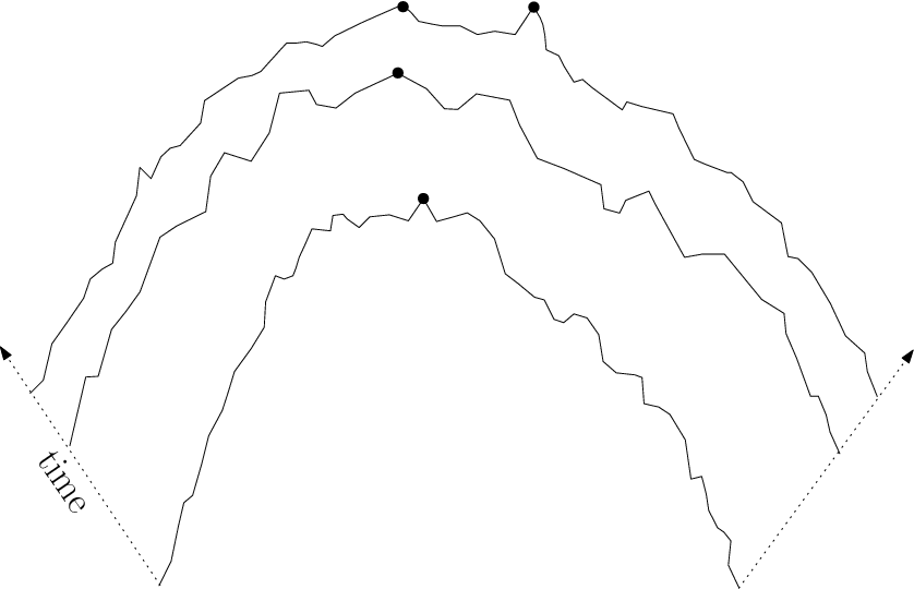
Figure 3. The KPZ fixed point 𝔥t​(x)\mathfrak{h}_{t}(x) spatial process depicted at three times; for clarity, we have shown the curves separated, but there need not be any ordering of the function values as time proceeds. The first two of the three times are typical ones at which the maximizer is unique (see the black bullet at its location), while the third is exceptional. There are then two maximizers, one close to those earlier and the other at a dramatic remove.

As we have mentioned, one of our results will be that 𝔥t​(x)\mathfrak{h}_{t}(x) attains its maximum at a unique location almost surely for each fixed t>0t>0 under general initial data. However, this does not preclude the existence of random exceptional times at which 𝔥t\mathfrak{h}_{t} has several maximizers. A classical example of a non-empty set of exceptional times is the zero set 𝖹𝖾𝗋𝗈={t≥0:B⁡(t)=0}\mathsf{Zero}=\{t\geq 0:B(t)=0\} of standard Brownian motion BB. For every T>0T>0, the Hausdorff dimension of 𝖹𝖾𝗋𝗈∩[0,T]\mathsf{Zero}\cap[0,T] is almost surely 12\frac{1}{2}—see [MP10, Theorem 4.24]. The random geometry of an exceptional time is trivial in this case—we merely have B⁡(t)=0B(t)=0 at such times. In our case, and others, there is however a rich geometry associated to exceptional times.

Indeed, the study of random dynamics that leaves invariant an equilibrium measure, and the question of the existence and Hausdorff dimension of an exceptional set of times at which an almost sure property of the equilibrium law is violated, are celebrated topics in modern probability theory. Discrete Fourier analytic tools have been employed to investigate [BKS99] the sensitivity to noise of critical percolation. This led to the proof [SS10] that, under a natural dynamic which left the critical percolation distribution invariant, there exist exceptional times where there exists an infinite cluster; further, the Hausdorff dimension of these exceptional times has been identified [GPS10] as 31/3631/36.

In our case, we will consider exceptional times when the 𝔥t\mathfrak{h}_{t} fails to have a unique maximizer. They can be viewed as moments of instability in the life of the random polymer, at which its endpoint loses its uniqueness. At such moments, the polymer’s future is uncertain, with the passage of even an instant of further time being liable to propel the polymer endpoint to a macroscopic distance from its present location (see Figures 2 and 3). (This does not contradict existing results on the continuity properties ofsuchpolymers, eg. from [DOV18], as those results are typically stated on the event that the polymer is unique.)

Let T>0T>0 and A≥0A\geq 0. The exceptional set of random times in [0,T][0,T] that are such moments of instability, when the polymer endpoint may subsequently jump by a distance greater than AA, is

(1.9) 𝒯T,A(𝔥):={t∈[0,T]:∃x1,x2∈Argmax(𝔥t),|x1−x2|>A},\mathcal{T}_{T,A}(\mathfrak{h}):=\bigl\{t\in[0,T]:\exists\,x_{1},x_{2}\in\mathrm{Argmax}(\mathfrak{h}_{t}),\;|x_{1}-x_{2}|>A\bigr\},

where the set Argmax⁡(𝔥t)⊂ℝ\mathrm{Argmax}(\mathfrak{h}_{t})\subset\mathbb{R} contains all points xx at which 𝔥t​(x)\mathfrak{h}_{t}(x) is the maximum value of 𝔥t\mathfrak{h}_{t}. When A=0A=0, we adopt the shorthand 𝒯T\mathcal{T}_{T} for 𝒯T,0\mathcal{T}_{T,0}; in this case, the condition on x1,x2x_{1},x_{2} may be equivalently written as x1≠x2x_{1}\neq x_{2}.

Of course, the set 𝒯T\mathcal{T}_{T} is random and depends on the initial data 𝔥0\mathfrak{h}_{0} of the KPZ fixed point. For example, if 𝔥0\mathfrak{h}_{0} does not have sufficiently fast decay at infinity, then 𝔥t\mathfrak{h}_{t} can be unbounded, in which case 𝒯T​(𝔥)\mathcal{T}_{T}(\mathfrak{h}) is empty. We thus need to impose some assumptions on the initial data 𝔥0\mathfrak{h}_{0} to ensure that our question is well-defined. For instance, we need that 𝔥t\mathfrak{h}_{t} is always almost surely bounded so that maximizers exist. We impose a slightly stronger condition, that 𝔥0\mathfrak{h}_{0} decays in a square-root manner at infinity and is identically −∞-\infty for all sufficiently negative arguments.

Assumption 1.1.

(Decay at infinity) The initial data 𝔥0:ℝ→[−∞,∞)\mathfrak{h}_{0}:\mathbb{R}\to[-\infty,\infty) of the KPZ fixed point is a non-random, upper semicontinuous function that is not identically equal to −∞-\infty, and for which (a) there exist α∈ℝ\alpha\in\mathbb{R} and γ>0\gamma>0 such that the bound 𝔥0​(y)≤α−γ​|y|1/2\mathfrak{h}_{0}(y)\leq\alpha-\gamma|y|^{1/2} holds for all y∈ℝy\in\mathbb{R} and (b) there exists λ∈ℝ\lambda\in\mathbb{R} such that 𝔥0​(y)=−∞\mathfrak{h}_{0}(y)=-\infty for y≤−λy\leq-\lambda.

Assumption 1.1 will refer to both parts (a) and (b), and we will occasionally make use of only part (a).

We will show in Lemma 3.1 that Assumption 1.1(a) guarantees that, at any time t>0t>0, the KPZ fixed point 𝔥t\mathfrak{h}_{t} is almost surely bounded and decays at infinity. This yields the existence of maximizers and leads to the natural question of their almost sure uniqueness at fixed times, a form of Johansson’s conjecture for general initial data; here is our result affirming this general form of the conjecture.

Theorem 1.2.

Let the initial data of the KPZ fixed point 𝔥0\mathfrak{h}_{0} satisfy Assumption 1.1(a). Then 𝔥t\mathfrak{h}_{t} has a unique maximizer almost surely for every fixed t>0t>0.

Theorem 1.2 should be provable by using the recent result of [SV20] which shows the absolute continuity of 𝔥t\mathfrak{h}_{t} with respect to Brownian motion on compact intervals. Such a proof would closely follow the original proof of Johansson’s conjecture in the narrow-wedge case presented in [CH14]; this requires a statement such as Lemma 3.1 on the decay of 𝔥t\mathfrak{h}_{t} at infinity. Our proof of Theorem 1.2, however, is independent of [SV20] and relies on the formulas for the KPZ fixed point proved in [MQR21]. In this way, it is more in line with the approach to Johansson’s conjecture in the narrow-wedge case presented in [FQR13]. However, in contrast to [FQR13], where a density of one maximizer was computed, from which uniqueness was concluded, we compute the probability that two maximizers appear at a given time and show that it equals zero.

Theorem 1.2 implies that the Lebesgue measure of 𝒯T,A​(𝔥)\mathcal{T}_{T,A}(\mathfrak{h}) is zero almost surely. It is thus natural to examine the fractal dimension of the exceptional set of violating times. We refer to Appendix A for the definition of the Hausdorff dimension dim(X)\dim(X) for a set X⊂ℝX\subset\mathbb{R}, because it is this notion of dimension that we will use to measure the exceptional set when it is non-empty. Our first result concerns the Hausdorff dimension of the set 𝒯T,A​(𝔥)\mathcal{T}_{T,A}(\mathfrak{h}) and proves an upper bound.

Theorem 1.3.

Let the initial data of the KPZ fixed point 𝔥0\mathfrak{h}_{0} satisfy Assumption 1.1. Then, for any T>0T>0 and A≥0A\geq 0,

(1.10) ℙ𝔥0​(dim(𝒯T,A​(𝔥))≤23)= 1.\mathbb{P}_{\mathfrak{h}_{0}}\Bigl(\dim(\mathcal{T}_{T,A}(\mathfrak{h}))\leq\tfrac{2}{3}\Bigr)\,=\,1.

In fact, we obtain the upper bound on the Hausdorff dimension under only Assumption 1.1(a). In our approach, we require the full Assumption 1.1 to show a lower bound on the probability of the existence of multiple near-maximizers at a given time, which we will shortly state as Theorem 1.6, because of a restriction in a “melon” transformation in Brownian last passage percolation that we rely on; we will say a little more about this transformation in Section 1.5, and about the restriction that it imposes in Section 5. We do not attempt the extension to more general initial data in the present article. We explain the difficulties in obtaining a matching lower bound on the Hausdorff dimension in Section 1.6.

Finally, in the case of narrow wedge initial data, we observe that it satisfies Assumption 1.1 and so we obtain the following corollary immediately.

Corollary 1.4.

For narrow wedge initial data 𝔥0=𝔡0\mathfrak{h}_{0}=\mathfrak{d}_{0} and for any T>0T>0,

(1.11) ℙ𝔡0​(dim(𝒯T​(𝔥))≤23)= 1.\mathbb{P}_{\mathfrak{d}_{0}}\Bigl(\dim(\mathcal{T}_{T}(\mathfrak{h}))\leq\tfrac{2}{3}\Bigr)\,=\,1.

1.3. Quantitative upper and lower bounds on near-twin peaks

Theorem 1.3 is the consequence of an upper bound on the probability that 𝔥t\mathfrak{h}_{t}, for given t>0t>0, satisfies an almost twin peaks condition. To our knowledge these are the first results giving explicit probability bounds for the KPZ fixed point under general initial data, and may prove to be of independent interest. Indeed, (weaker) upper bounds on similar twin peaks probabilities in the narrow-wedge case were obtained in [CHH19, GH20] and used in [GH20a] in the related context of Brownian LPP to understand a phase transition under a particular dynamic.

Let us define what we mean by an almost twin peaks more precisely. For ε>0\varepsilon>0 and fixed β∈(0,1)\beta\in(0,1), define the ε\varepsilon-twin peaks set 𝖳𝖯A,Lε\mathsf{TP}_{\!\!A,L}^{\varepsilon} by

(1.12) 𝖳𝖯A,Lε={f:ℝ→ℝ∪−∞:|Max(f)|≤(βL)1/2,𝖲A,Lε(f)≠∅},\mathsf{TP}_{\!\!A,L}^{\varepsilon}=\left\{f:\mathbb{R}\to\mathbb{R}\cup{-\infty}:|\mathrm{Max}(f)|\leq(\beta L)^{1/2},\mathsf{S}_{A,L}^{\varepsilon}(f)\neq\varnothing\right\},

where

𝖲A,Lε(f):={(x1,x2)∈[−βL,βL]2:x2−x1>A,Max(f)−f(xi)≤εfori=1,2}.\mathsf{S}_{A,L}^{\varepsilon}(f):=\Bigl\{(x_{1},x_{2})\in[-\beta L,\beta L]^{2}:x_{2}-x_{1}>A,\;\mathrm{Max}(f)-f(x_{i})\leq\varepsilon~\text{for}~i=1,2\Bigr\}.

In words, 𝖳𝖯A,Lε\mathsf{TP}_{\!\!A,L}^{\varepsilon} is the event of having two locations, in an interval of length of order LL, at distance at least AA apart, where the value of 𝔥t(n)\mathfrak{h}^{{\scriptscriptstyle(}n{\scriptscriptstyle)}}_{t} is within ε\varepsilon of the global maximum; additionally, the maximum is in absolute value at most of order L1/2L^{1/2}.

The upper bound on the Hausdorff dimension can be proved by understanding the probability of exhibiting an ε\varepsilon-twin peaks at time tt, which is our next main result. Here, we use the cut-off 𝔥tL\mathfrak{h}_{t}^{L} of the KPZ fixed point, which is essentially 𝔥t|[−L,L]\mathfrak{h}_{t}|_{[-L,L]}; it is defined in (3.12).

Theorem 1.5.

Let the initial data 𝔥0∈UC\mathfrak{h}_{0}\in\UC of the KPZ fixed point satisfy 𝔥0​(x)≤α\mathfrak{h}_{0}(x)\leq\alpha for some α∈ℝ\alpha\in\mathbb{R} and for any x∈ℝx\in\mathbb{R}. Then, for any 0<L≤L¯0<L\leq\bar{L}, A>0A>0 and 0<T0<T0<T_{0}<T,

(1.13) ℙ𝔥0​(𝔥tL∈𝖳𝖯A,L¯ε)≤C​ε​t−13,\mathbb{P}_{\mathfrak{h}_{0}}\Bigl(\mathfrak{h}^{L}_{t}\in\mathsf{TP}_{\!\!A,\bar{L}}^{\varepsilon}\Bigr)\leq C\varepsilon t^{-\frac{1}{3}},

for t∈[T0,T]t\in[T_{0},T] and ε∈(0,1)\varepsilon\in(0,1), and for a constant C≥0C\geq 0 depending on T0T_{0}, L¯\bar{L}, AA, β\beta (which comes into the definition (1.12)) and α\alpha (i.e., the dependence on 𝔥0\mathfrak{h}_{0} is merely via the constant α\alpha).

Observe that this theorem immediately yields Theorem 1.2 by taking ε→0\varepsilon\to 0 and then L,L¯,A→∞L,\bar{L},A\to\infty.

As we will see in the proof outline section ahead, the Hausdorff dimension upper bound of 23\frac{2}{3} that we prove is a consequence of the 13\frac{1}{3} exponent of tt and 11 exponent of ε\varepsilon in the previous result. In the next result we show that the ε\varepsilon-dependence is sharp by proving a matching lower bound.

Theorem 1.6.

Let the initial state 𝔥0\mathfrak{h}_{0} of the KPZ fixed point satisfy Assumption 1.1, and suppose that A>0A>0 and t>0t>0. There exist L0L_{0} and c′>0c^{\prime}>0 (both depending on AA, tt, and 𝔥0\mathfrak{h}_{0}) such that, for all L≥L0L\geq L_{0} and ε∈(0,1)\varepsilon\in(0,1),

(1.14) ℙ𝔥0​(𝔥t∈𝖳𝖯A,Lε)≥c′​ε.\mathbb{P}_{\mathfrak{h}_{0}}\Bigl(\mathfrak{h}_{t}\in\mathsf{TP}_{\!\!A,L}^{\varepsilon}\Bigr)\geq c^{\prime}\varepsilon.

Further, c′c^{\prime} and L0L_{0} can be taken to depend on t>0t>0 in a continuous manner.

1.4. A density of two maximizers

Our proof of Theorem 1.5 relies on existence of the joint density of two maximizers and the maximal value of the KPZ fixed point 𝔥t\mathfrak{h}_{t}. More precisely, for t,L>0t,L>0 and M∈ℝM\in\mathbb{R}, define the function

(1.15) ℱt,M,L(η1;η2)​(x1,x2):=ℙ𝔥0​(For each ​i∈{1,2},𝔥t​(yi)>M−εi​ forCLOSE\displaystyle\mathcal{F}_{t,M,L}^{(\eta_{1};\eta_{2})}(x_{1},x_{2}):=\mathbb{P}_{\mathfrak{h}_{0}}\Big(\text{For each }i\in\{1,2\},\,\,\mathfrak{h}_{t}(y_{i})>M-\varepsilon_{i}\text{ for}
(1.16) some yi∈[xi,xi+δi), and 𝔥t(z)≤M for z∈[−L,L]),\displaystyle\text{ some }y_{i}\in[x_{i},x_{i}+\delta_{i}),\text{ and }\mathfrak{h}_{t}(z)\leq M\text{ for }z\in[-L,L]\Big),

where ηi=(εi,δi)\eta_{i}=(\varepsilon_{i},\delta_{i}) with εi,δi>0\varepsilon_{i},\delta_{i}>0. Here, we have suppressed dependence on the initial data 𝔥0\mathfrak{h}_{0}. The function ℱt,M,L(η1;η2)​(x1,x2)\mathcal{F}_{t,M,L}^{(\eta_{1};\eta_{2})}(x_{1},x_{2}) equals the probability that the KPZ fixed point visits ε1\varepsilon_{1}- and ε2\varepsilon_{2}-neighbourhoods of its maximum in δ1\delta_{1}- and δ2\delta_{2}-neighbourhoods around the respective points x1x_{1} and x2x_{2}, with the maximum being close to MM. The next result implies that properly normalized functions ℱt,M,L(η1;η2)​(x1,x2)\smash{\mathcal{F}^{(\eta_{1};\eta_{2})}_{t,M,L}(x_{1},x_{2})} converge to a non-trivial limit as η1,η2↘0\eta_{1},\eta_{2}\searrow 0. To compute the limit of this function, we fix a constant α⋆>12\alpha_{\star}>\frac{1}{2}; define the domain

(1.17) 𝖣𝗈𝗆:={(ε,δ)∈ℝ2:δ>0, 0<ε≤δα⋆};\mathsf{Dom}:=\bigl\{(\varepsilon,\delta)\in\mathbb{R}^{2}\,:\,\delta>0,\,0<\varepsilon\leq\delta^{\alpha_{\star}}\bigr\};

and denote the limit in this domain

(1.18) limη↘0~​f​(η):=limη∈𝖣𝗈𝗆,η↘0⁡f⁡(η),\underset{\eta\searrow 0}{\widetilde{\mathrm{lim}}}f(\eta):=\mathop{\mathop{\text{{lim}}}}\displaylimits_{\eta\in\mathsf{Dom},\,\eta\searrow 0}f(\eta),

for a suitable function ff. It should be noted that, when we take the limit η↘0\eta\searrow 0, we are implicitly claiming that the double limit in ε\varepsilon and δ\delta in 𝖣𝗈𝗆\mathsf{Dom} exists and does not depend on how that limit is performed.

Theorem 1.7.

Assume that the initial data of the KPZ fixed point satisfies 𝔥0​(x)≤α\mathfrak{h}_{0}(x)\leq\alpha for some α∈ℝ\alpha\in\mathbb{R} and for all x∈ℝx\in\mathbb{R}. For every fixed t>0t>0 the following limit exists:

(1.19) ℱt,M​(x1,x2):=limL→∞⁡limη1↘0~​limη2↘0~​1ε1​δ1​ε2​δ2​ℱt,M,L(η1;η2)​(x1,x2),\mathcal{F}_{t,M}(x_{1},x_{2}):=\mathop{\mathop{\text{{lim}}}}\displaylimits_{L\to\infty}\ \underset{\eta_{1}\searrow 0}{\widetilde{\mathrm{lim}}}\ \underset{\eta_{2}\searrow 0}{\widetilde{\mathrm{lim}}}\ \frac{1}{\varepsilon_{1}\delta_{1}\varepsilon_{2}\delta_{2}}\mathcal{F}^{(\eta_{1};\eta_{2})}_{t,M,L}(x_{1},x_{2}),

pointwise for x1,x2∈(−L,L)x_{1},x_{2}\in(-L,L) and M∈ℝM\in\mathbb{R}, such that x2−x1>0x_{2}-x_{1}>0. Further, ℱt,M\mathcal{F}_{t,M} satisfies a scale invariance property:

(1.20) ℱt,M(x1,x2)=t−2ℱ1,t−1/3M(t−23x1,t−23x2),\mathcal{F}_{t,M}(x_{1},x_{2})=t^{-2}\mathcal{F}_{1,t^{-1/3}M}\bigl(t^{-\frac{2}{3}}x_{1},t^{-\frac{2}{3}}x_{2}\bigr),

where the right-hand function is defined for the initial data 𝔥0(t)(x):=t−1/3𝔥0(t2/3x)\mathfrak{h}_{0}^{(t)}(x):=t^{-1/3}\mathfrak{h}_{0}(t^{2/3}x). Moreover, this function can be written explicitly as

(1.21) ℱ1,M​(x1,x2)=det⁡(I−𝐊1/2hypo⁡(𝔥0)​(𝐑−𝐀(0,⋆)−𝐀(⋆,0)+𝐀(⋆,⋆)))−det(I−𝐊hypo⁡(𝔥0)1/2(𝐑−𝐀(0,⋆)))−det(I−𝐊hypo⁡(𝔥0)1/2(𝐑−𝐀(⋆,0)))+det(I−𝐊hypo⁡(𝔥0)1/2𝐑),\begin{split}\mathcal{F}_{1,M}(x_{1},x_{2})&=\mathop{\mathop{\text{{det}}}}\nolimits\Bigl(I-\mathbf{K}^{\hypo(\mathfrak{h}_{0})}_{1/2}\Bigl(\mathbf{R}-\mathbf{A}^{(0;\star)}-\mathbf{A}^{(\star;0)}+\mathbf{A}^{(\star;\star)}\Bigr)\Bigr)\\ &\quad-\mathop{\mathop{\text{{det}}}}\nolimits\Bigl(I-\mathbf{K}^{\hypo(\mathfrak{h}_{0})}_{1/2}\Bigl(\mathbf{R}-\mathbf{A}^{(0;\star)}\Bigr)\Bigr)\\ &\quad-\mathop{\mathop{\text{{det}}}}\nolimits\Bigl(I-\mathbf{K}^{\hypo(\mathfrak{h}_{0})}_{1/2}\Bigl(\mathbf{R}-\mathbf{A}^{(\star;0)}\Bigr)\Bigr)+\mathop{\mathop{\text{{det}}}}\nolimits\Bigl(I-\mathbf{K}^{\hypo(\mathfrak{h}_{0})}_{1/2}\mathbf{R}\Bigr),\end{split}

where the kernels in the Fredholm determinants are defined in (2.12) and Section 4.1.5.

(To be precise, the function ℱ1,M\mathcal{F}_{1,M} should be called a super-density, because its integral over the arguments x1x_{1}, x2x_{2} and MM exceeds 11; in fact, we expect this integral to be infinite.)

1.5. Heuristics and structure

We will indicate three main facts; how they will combine into a proof of the upper bound of the Hausdorff dimension of the exceptional set and the non-emptiness of that set; and, in outline, how we will prove each of them. In so doing, we will indicate the structure of the paper, which is also illustrated in Figure 4.

In a crude but instructive simplification, a set has dimension α\alpha if, for any ε>0\varepsilon>0, it may be fattened to become a union of order ε−α\varepsilon^{-\alpha} intervals of length ε\varepsilon. The fattened set will be a proxy set 𝒯Tε​(𝔥)={t≤T:𝔥t∈𝖳𝖯ε}\mathcal{T}_{T}^{\varepsilon}(\mathfrak{h})=\{t\leq T:\mathfrak{h}_{t}\in\mathsf{TP}^{\varepsilon}\}; namely, the set of times tt at which the KPZ fixed point 𝔥t\mathfrak{h}_{t} lies in the twin peaks set 𝖳𝖯ε\mathsf{TP}^{\varepsilon} (similar to 𝖳𝖯A,Lε\mathsf{TP}_{\!\!A,L}^{\varepsilon} introduced earlier) of upper semicontinuous functions ff such that Max⁡(f)−f⁡(xi)≤ε\mathrm{Max}(f)-f(x_{i})\leq\varepsilon for some points x1,x2∈ℝx_{1},x_{2}\in\mathbb{R} such that |x1−x2|≥1|x_{1}-x_{2}|\geq 1. We refer to these points x1x_{1} and x2x_{2} as near maximizers. The reader may recall that in our earlier statements of bounds on the probability of 𝔥t\mathfrak{h}_{t} lying in 𝖳𝖯A,Lε\mathsf{TP}_{\!\!A,L}^{\varepsilon}, we consider near maximizers whose distance |x1−x2||x_{1}-x_{2}| is at least a given small value AA; and for which |x1|,|x2|≤L|x_{1}|,|x_{2}|\leq L for large LL. In this present heuristic discussion, we ignore these variables. Here are the three main facts that we demonstrate:

  1. (i)

    The KPZ fixed point 𝔥t​(x)\mathfrak{h}_{t}(x) is Hölder-13−\tfrac{1}{3}^{{\scriptscriptstyle-}} in tt, uniformly over compact sets in xx.

  2. (ii)

    The probability that 𝔥t∈𝖳𝖯ε\mathfrak{h}_{t}\in\mathsf{TP}^{\varepsilon} is at most Cεt−1/3C\varepsilon t^{-1/3} (Theorem 1.5).

  3. (iii)

    The same probability is at least C⁡(t)​εC(t)\varepsilon (Theorem 1.6).

(Strictly speaking, only the first two points are needed for an upper bound on the dimension. The third point aids in the heuristic explanation of why the dimension should be equal to 23\frac{2}{3}, and would be needed to prove a matching dimension lower bound; see Section 1.6 ahead for why are unable to do this.)

Given these, we may see why the Hausdorff dimension of 𝒯T​(𝔥)\mathcal{T}_{T}(\mathfrak{h}) will be two-thirds when this set is non-empty. Indeed, Item (i) implies that the maximum of 𝔥t\mathfrak{h}_{t} is Hölder 13−\frac{1}{3}^{\scriptscriptstyle-} in time, which suggests that intervals contained in 𝒯Tε​(𝔥)\mathcal{T}_{T}^{\varepsilon}(\mathfrak{h}) should typically be at least of size of order ε3\varepsilon^{3}. Item (ii) gives us a complementary upper bound on the typical length of intervals in 𝒯Tε​(𝔥)\mathcal{T}_{T}^{\varepsilon}(\mathfrak{h}). In particular, it shows that, once the set 𝒯Tε​(𝔥)\mathcal{T}_{T}^{\varepsilon}(\mathfrak{h}) is entered, in the passage of time of order ε3\varepsilon^{3}, it will be exited (and hence the interval will have ended). Finally, Item (iii) along with Item (ii) implies that the total size of 𝒯Tε​(𝔥)\mathcal{T}_{T}^{\varepsilon}(\mathfrak{h}) is of order ε\varepsilon. Thus, 𝒯Tε​(𝔥)\mathcal{T}_{T}^{\varepsilon}(\mathfrak{h}) is a set of size ε\varepsilon which consists of intervals of length ε3\varepsilon^{3}; the number of intervals must be of order ε−2\varepsilon^{-2}, and such an order of intervals of length ε\varepsilon will be needed to cover 𝒯T​(𝔥)\mathcal{T}_{T}(\mathfrak{h}). The infimum ℋεα​(𝒯T​(𝔥))\mathcal{H}^{\alpha}_{\varepsilon}(\mathcal{T}_{T}(\mathfrak{h})) of α\alpha-values of coverings of maximum diameter ε\varepsilon recalled in (A.1) should be of order ε−2+3​α\varepsilon^{-2+3\alpha}, a quantity whose behavior changes as ε→0\varepsilon\to 0 depending on whether α\alpha is greater or less than 2/32/3. Thus is the Hausdorff dimension of two-thirds predicted. Of course, we only prove an upper bound of two-thirds; see ahead in Section 1.6 for a discussion of where our methods face difficulties in proving a lower bound.

Our task is thus to prove the three facts. The respective proofs appear in Sections 3, 4, and 5. The first two pieces are fit together to prove Theorem 1.3 in the final Section 6. Next we explain in outline how the three tasks will be accomplished.

Lemma 3.4 is the precise rendering of Item (i). That 𝔥t​(x)\mathfrak{h}_{t}(x) is Hölder-13−\frac{1}{3}^{\scriptscriptstyle-} in tt for fixed xx is known from [MQR21], but our proof of the extra local uniformity in space makes use of a variational formula, recalled in Section 2, for the KPZ fixed point in terms of the directed landscape recently constructed in [DOV18]. The proof also requires that 𝔥t​(x)\mathfrak{h}_{t}(x) is Hölder-12−\frac{1}{2}^{\scriptscriptstyle-} in xx, locally uniformly in tt, which we prove in Lemma 3.2. Finally, the spatially uniform temporal continuity’s implication that Max⁡(𝔥t)\mathrm{Max}(\mathfrak{h}_{t}) is Hölder-13−\frac{1}{3}^{\scriptscriptstyle-} in time is recorded in Lemma 3.5.

The previously stated Theorem 1.5 is the rigorous manifestation of Item (ii), and is derived by way of a density whose existence is asserted in Theorem 1.7. The much more involved proof of these results uses exact formulas, also recalled in Section 2, for the KPZ fixed point in terms of Fredholm determinants that have been obtained in [MQR21]. More precisely, for a fixed t>0t>0 and for any δ,ε>0\delta,\varepsilon>0, we will consider in (1.16) the probability that two near maximizers of 𝔥t\mathfrak{h}_{t} are located in δ\delta-neighbourhoods of fixed points x1≠x2x_{1}\neq x_{2}, while the maximum of 𝔥t\mathfrak{h}_{t} is in an ε\varepsilon-neighbourhood of a fixed value MM. Dividing this probability by δ2​ε2\delta^{2}\varepsilon^{2} and taking the limits ε,δ→0\varepsilon,\delta\to 0, we will obtain in effect the density, conditionally on maximizer non-uniqueness, of the maximum value and two maximizers of 𝔥t\mathfrak{h}_{t}; this is the limit and the density whose existence is the content of Theorem 1.7. In Proposition 4.1, scaling properties and bounds on this limit are asserted. (To call this just mentioned limit a density is really an improper formulation because the concerned law is σ\sigma-finite, with infinite mass on maximizer pairs at distance close to zero.) The derivation of this result involves double differentiation of a Fredholm determinant, arising from the distribution function of the KPZ fixed point. The justification of this differentiation and the computation of the derivatives are quite technical, involving asymptotic analysis of path integral formulations of the Fredholm determinant kernels, defined by means of a Brownian scattering transform. These calculations rely on properties of trace class operators and Fredholm determinants that are summarized in Appendix B; and bounds on kernels involving Airy functions that are reviewed in Appendix C.

Theorem 1.5 is then obtained by integration of the just indicated density function over x1x_{1}, x2x_{2} and MM. Combining Item (ii) with the temporal Hölder regularity of 𝔥t\mathfrak{h}_{t} and of its maximum, given in Item (i), yields the upper bound on the Hausdorff dimension of 𝒯T​(𝔥)\mathcal{T}_{T}(\mathfrak{h}).

Theorem 1.6 is the precise rendering of Item (iii). Its proof, in contrast to that of Item (ii), relies on a Gibbsian resampling argument, akin in spirit to the Brownian Gibbs property used in such works as [CH14, DV21, Ham22, CHH19]; we discuss this property in greater detail in Section 5. The argument works in the prelimiting model of Brownian last passage percolation: the random variable 𝔥t(n)\smash{\mathfrak{h}^{{\scriptscriptstyle(}n{\scriptscriptstyle)}}_{t}}, namely the prelimiting version of 𝔥t\mathfrak{h}_{t}, will be written in terms of a last passage value through a random environment obtained by a “melon” transformation of the original Brownian environment (the term “melon” is used in [DOV18], though one could instead call this a “continuous RSK correspondence” or a “Pitman transform”). This relies on a remarkable identity of last passage values through the original and melon-transformed environments proved in [DOV18]. (The identity was later found to be implied by the earlier work [NY04] in the more general setting of positive temperature polymer models; see [Cor21] for more details and three proofs of the positive temperature identity, and [Dau22] for a fourth). It is through this melon transform that we are able to access general initial data.

The melon transformed environment coincides with Dyson Brownian motion with β=2\beta=2. This ensemble of random curves is Gibbsian, enjoying a simple Brownian resampling invariance. By harnessing this invariance, we may exploit the melon-transformed environment, resampling 𝔥t(n)\smash{\mathfrak{h}^{{\scriptscriptstyle(}n{\scriptscriptstyle)}}_{t}} in order to generate an event of probability at least C2​εC_{2}\varepsilon on which 𝔥t(n)∈𝖳𝖯ε\smash{\mathfrak{h}^{{\scriptscriptstyle(}n{\scriptscriptstyle)}}_{t}\in\mathsf{TP}^{\varepsilon}}. Taking n→∞n\to\infty is the final step on the road to Theorem 1.6.

The lower bound in Item (iii) is suggested by (but does not follow from) the spatial Brownian absolute continuity of 𝔥t\mathfrak{h}_{t} established in [SV20]. Indeed, a Brownian bridge has probability proportional to ε\varepsilon of having a unit-order separated location that comes within ε\varepsilon of the maximal value of the bridge. A much more quantitative comparison result than absolute continuity is needed, however, in order to transfer small probability events between the Brownian measure and the spatial process for 𝔥t\mathfrak{h}_{t}. Our approach does not seek such a comparison, but rather attacks the problem directly.

Although Gibbsian resampling is not a new technique in studying models in the KPZ universality class, our use of it departs from existing methods in two quite substantial ways. In previous works obtaining quantitative probability bounds on KPZ objects via Gibbs resampling, the Gibbsian line ensemble which is being resampled is the object of interest. In the present work, we are interested in last passage percolation in the environment defined by the Gibbsian line ensemble. If we restrict attention to narrow wedge initial data, we recover the earlier considered cases where the line ensemble is the object of interest (i.e., the last passage problem trivializes). (Of course, a number of other works, such as [DOV18], have made use of resampling arguments with the line ensemble to obtain important qualitative results—indeed, we crucially rely on the important identity from [DOV18] mentioned above.) The second departure is that our resampling is performed on a random interval defined relative to the location of the unique global maximizer. In this sense, the resampling may be called non-Markovian. To illustrate the complication that this introduces, consider a Brownian bridge. Its law on any given interval is invariant under replacing the path by an independent Brownian bridge affinely shifted to fit in. If we look at its law on an interval starting at the maximizer of the path, such a resampling invariance no longer holds. To handle this in the Brownian bridge case, as well as in our more general case, we rely on a path decomposition of Markov processes at certain special times given in [Mil78].

The Hausdorff dimension of exceptional times is at most 23\frac{2}{3} (Theorem 1.3) The KPZ fixed point is a.s. bounded (Lemma 3.1) The max of the KPZ fixed point is 13−\tfrac{1}{3}^{{\scriptscriptstyle-}}-Hölder (Lemma 3.5) The probability that 𝔥t∈𝖳𝖯ε\mathfrak{h}_{t}\in\mathsf{TP}^{\varepsilon} is at most Cεt−1/3C\varepsilon t^{-1/3} (Theorem 1.5) The probability that 𝔥t∈𝖳𝖯ε\mathfrak{h}_{t}\in\mathsf{TP}^{\varepsilon} is at least C⁡(t)​εC(t)\varepsilon (Theorem 1.6) The KPZ fixed point formula and its properties (Propositions 2.3 & 2.4) Existence and properties of the density of two maximizers (Proposition 4.1) Properties of the directed landscape (Proposition 2.2)
Figure 4. Flowchart of the paper. The grey blocks correspond to the three items described in Section 1.5.

1.6. The difficulty in proving a matching lower bound

Typically in proving bounds on Hausdorff dimension, the lower bound is the harder one to prove, and it is the same here. We try to give an indication now of why our methods face difficulties in proving a lower bound.

The basic problem is in understanding the behavior of the KPZ fixed point at very small times in a uniform way. In particular, to obtain a lower bound on the Hausdorff dimension, one needs to have some control on the probability of two times lying in 𝒯T,A\mathcal{T}_{T,A}, where the two times may be arbitrarily close. By the Markov property of the fixed point, this is equivalent to understanding the probability that t∈𝒯T,At\in\mathcal{T}_{T,A} for arbitrarily small tt from an initial condition taken from a fairly wide class, which we approach by studying the probability that 𝔥t∈𝖳𝖯Aε\mathfrak{h}_{t}\in\mathsf{TP}_{\!\!A}^{\varepsilon} for small ε\varepsilon.

Heuristically, if the initial condition is very flat, there are many locations from which a potential maximizer can arise, which would increase the probability that 𝔥t∈𝖳𝖯Aε\mathfrak{h}_{t}\in\mathsf{TP}_{\!\!A}^{\varepsilon} for small tt (when the parabolic decay effect of the fixed point is weaker). And indeed, Theorem 1.5 provides a bound only when tt is bounded away from zero—a technically precise version of the problem.

Our approach to obtaining the upper bound in Theorem 1.5 has been by way of integrating the density from Theorem 1.7; the density is a joint density of the location of the maximizers and the value of the maximum. On a technical level, the problem we face is that the density blows up when the maximum value argument is taken to −∞-\infty; by KPZ scaling, as t→0t\to 0, the maximum value being larger than a negative constant −M-M at time tt is the same as it being greater than −Mt−1/3-Mt^{-1/3} at time 1, and so the maximum value argument must be allowed to go to −∞-\infty if we want to allow small tt. The blowup of the density in this regime is somewhat to be expected by our heuristic from the previous paragraph: when the maximum is very negative, the shape of the profile should be essentially flat on a large interval. And it is this density blowup which leads to the imposition that tt be away from zero in Theorem 1.5. For the same reason, our bounds do not imply that the set of exceptional times is non-empty with positive probability.

A similar problem was encountered in [Dau22a], who adopted a thinning procedure and an understanding of the envelope of growth (a law of iterated logarithm) for the KPZ fixed point at short times, which sufficed to handle the problem in the context of the argument framework developed there. We discuss the approach of [Dau22a] a bit more in Section 1.8.

1.7. Conjectures for some related exceptional sets

Theorem 1.3 offers an assertion concerning fractal geometry for exceptional sets embedded in the KPZ fixed point. Several assertions may naturally be conjectured concerning related fractals embedded either in the KPZ fixed point or in the space-time Airy sheet. Here we state, and explain the reasoning for, some such conjectures. Our first conjecture concerns more basic structural properties of the set 𝒯T\mathcal{T}_{T} than its dimension.

Conjecture 1.8.

For any 𝔥0\mathfrak{h}_{0} satisfying Assumption 1.1, 𝒯∞​(𝔥)\mathcal{T}_{\infty}(\mathfrak{h}) is almost surely dense in [0,∞)[0,\infty).

Let us assume, for the moment, that we can show that for general initial data and any T>0T>0, 𝒯T≠∅\mathcal{T}_{T}\neq\varnothing almost surely. Then by the Markov property we can apply this result to the fixed point at any given time t>0t>0 by considering the process started with initial data given by 𝔥t\mathfrak{h}_{t}. This would imply that around any rational time, there is a time arbitrarily close when non-uniqueness holds—thus the almost sure density result.

In dynamical percolation at criticality on the faces of the honeycomb lattice [SS10, GPS10], the probability that a given face lies in an infinite open component at some time on a given unit interval is known to be bounded away from zero and one. However, the set of times at which there exists an infinite open component is presumably almost surely dense—and a zero-one law seems to promise such a result, though no such proof is recorded to our knowledge. Given our conjecture, we see an analogy between exceptional times for the KPZ fixed point at which two maximizers exist, separated to unit order, with times in dynamic percolation at which the infinite open cluster visits a given region; and between those exceptional times at which the pair of maximizers exist, without any demand of separation, and moments in dynamical percolation at which the infinite open cluster exists, without any condition being imposed on its geometry.

Our principal result, Theorem 1.3, concerns the Hausdorff dimension of exceptional times in the KPZ fixed point at which there exist two maximizers, and a natural question concerns the Hausdorff dimensions of times at which there are a given number of maximizers exceeding two. We formulate a conjecture on the values of these dimensions.

Conjecture 1.9.

The Hausdorff dimension of the set of times with three maximizers is one-third; the set of times with four such has zero Hausdorff dimension. For five maximizers, there almost surely exist no such exceptional times.

Admitting this conjecture, the set of times at which there exist four maximizers could be non-empty, but we believe this set to be empty almost surely.

Duncan Dauvergne has recently proven Conjectures 1.8 and 1.9 in [Dau22a]. In the case of four maximizers, he also shows that the set is either almost surely empty or almost surely dense.

We argue for Conjecture 1.9 in the case of three maximizers, developing the heuristic presented for the case of two in the preceding section. Let 𝒯T​(3)\mathcal{T}_{T}(3) denote the set of times with three maximizers, which, by a countability argument, we may suppose to be at mutual distance at least one; and let 𝒯Tε​(3)\mathcal{T}_{T}^{\varepsilon}(3) denote the set of times tt at which there exist three points at mutual distance at least one, for each of which, 𝔥t\mathfrak{h}_{t} is within ε\varepsilon of its maximum. Local Brownianity of 𝔥t\mathfrak{h}_{t} suggests that ℙ⁡(t∈𝒯Tε​(3))=Θ⁡(ε2)\mathbb{P}(t\in\mathcal{T}_{T}^{\varepsilon}(3))=\Theta(\varepsilon^{2}). Because 𝔥t\mathfrak{h}_{t} is 13−\tfrac{1}{3}^{{\scriptscriptstyle-}}-Hölder in time, 𝒯Tε​(3)\mathcal{T}_{T}^{\varepsilon}(3) may plausibly be decomposed into intervals of length of order ε3\varepsilon^{3}. Setting δ=ε3\delta=\varepsilon^{3}, the number of intervals of length δ\delta needed to cover 𝒯Tε​(3)\mathcal{T}_{T}^{\varepsilon}(3), and hence 𝒯T​(3)\mathcal{T}_{T}(3), should be of order ε2/ε3=ε−1=δ−1/3\varepsilon^{2}/\varepsilon^{3}=\varepsilon^{-1}=\delta^{-1/3}, whence our prediction.

Our results and the above conjectures concern the KPZ fixed point, in which the initial time is fixed at zero. The fractal geometry of exceptional sets may also be explored in the directed landscape ℒ\mathcal{L} constructed in [DOV18]. This landscape ascribes to any pair of points (y,s),(x,t)∈ℝ2(y,s),(x,t)\in\mathbb{R}^{2} with s<ts<t a random real-valued weight ℒ⁡(y,s,x,t)\mathcal{L}(y,s;x,t) that is a scaled expression for the energy in Brownian LPP of the geodesic whose route in scaled coordinates starts at (y,s)(y,s) and ends at (x,t)(x,t). A fractal object in the landscape is the difference profile ℝ→ℝ:z↦ℒ⁡(1,0,z,1)−ℒ⁡(−1,0,z,1)\mathbb{R}\to\mathbb{R}:z\mapsto\mathcal{L}(1,0;z,1)-\mathcal{L}(-1,0;z,1). This is a non-decreasing random function whose set of points of increase almost surely has Hausdorff dimension one-half [BGH21]. For generic point pairs (y,s),(x,t)∈ℝ2(y,s),(x,t)\in\mathbb{R}^{2} with s<ts<t, there is a unique path—the geodesic—that interpolates the pair’s elements whose scaled energy attains the value ℒ⁡(y,s,x,t)\mathcal{L}(y,s;x,t). Exceptionally, two such paths exist that are disjoint except at their shared endpoints. The set (x,y)∈ℝ2(x,y)\in\mathbb{R}^{2} for which (y,0)(y,0) and (x,1)(x,1) are such a pair of points has Hausdorff dimension one-half almost surely [BGH22].

To formulate conjectures that develop the theme of the present article but concern the coupling offered by the system ℒ\mathcal{L}, let XX denote the set of triples (y,s,t)(y,s,t) where y∈ℝy\in\mathbb{R} and s,t∈ℝs,t\in\mathbb{R} with s<ts<t. Each element indexes a scaled energy profile ℝ→ℝ:x↦ℒ⁡(y,s,x,t)\mathbb{R}\to\mathbb{R}:x\mapsto\mathcal{L}(y,s;x,t) which may, exceptionally, have several maximizers. Indeed, for k∈ℕk\in\mathbb{N} with k≥2k\geq 2, we may set EkE_{k} equal to the subset of elements of XX for which |s−t|≥1|s-t|\geq 1 and for which there are at least kk maximizers x1,…,xkx_{1},\ldots,x_{k} for which |xi−xj|≥1|x_{i}-x_{j}|\geq 1 for all 1≤i<j≤k1\leq i<j\leq k.

The space XX should be equipped with a metric if Hausdorff dimension questions are to be well-posed. A natural notion of distance on XX stipulates that the distance (y1,s1,t1)(y_{1},s_{1},t_{1}) and (y2,s2,t2)(y_{2},s_{2},t_{2}) equals |t1−t2|+|s1−s2|+|y1−y2|3/2|t_{1}-t_{2}|+|s_{1}-s_{2}|+|y_{1}-y_{2}|^{3/2} (this is not a metric as it does not satisfy the triangle inequality). The power of 3/23/2 in the final term accounts for the shape of a KPZ space-time box: if such a box has height ε3\varepsilon^{3}, it will have width ε2\varepsilon^{2}. Despite the mentioned notion of distance not being a metric, this specification of the radius of boxes can be used to define a scaling-adapted notion of Hausdorff measure and dimension. Such a scaling-adapted specification of a parabolic form of Hausdorff dimension was used by Cafferelli, Kohn and Nirenberg [CKN82] in their treatment of partial regularity of weak solutions of the Navier-Stokes’ equations.

Conjecture 1.10.

When XX is equipped with the just specified metric, the Hausdorff dimension of EkE_{k} is almost surely equal to max⁡{3−k/3,0}\mathop{\mathop{\text{{max}}}}\displaylimits\{3-k/3,0\}. Moreover, E10E_{10} is empty almost surely.

To make a case for the conjecture, let an ε\varepsilon-box in XX take the form of a rectangle whose length is ε3\varepsilon^{3} in the tt and ss coordinates, and ε2\varepsilon^{2} in the xx coordinate. Let Ek​(ε)E_{k}(\varepsilon) denote a fattening of the exceptional set EkE_{k}, wherein a given triple qualifies for membership if there exist kk points at pairwise distance at least one at which the indexed profile achieves a shortfall from its maximum of at most ε\varepsilon. By profile Brownianity on unit-order scales, we expect that the intersection of Ek​(ε)E_{k}(\varepsilon) with a unit-order ball in XX has Lebesgue measure εk−1\varepsilon^{k-1}. But the measure of an ε\varepsilon-box is ε3+3+2=ε8\varepsilon^{3+3+2}=\varepsilon^{8}. Thus, the number of boxes needed to cover Ek​(ε)E_{k}(\varepsilon) should be of order εk−9\varepsilon^{k-9}. The diameter δ\delta of an ε\varepsilon-box equals ε3\varepsilon^{3} in the metric we specified above. The number of boxes in the covering is thus δk/3−3\delta^{k/3-3}. This inference points to the sought conclusion that the Hausdorff dimension of EkE_{k} equals 3−k/33-k/3; provided, of course, that this quantity is not negative.

1.8. A brief discussion of [Dau22a]

As mentioned, [Dau22a] establishes Conjectures 1.8 and 1.9 as well as a stronger form of Theorem 1.3. Here we discuss how Dauvergne’s approach differs from ours.

The basic tool used in [Dau22a] is that almost sure statements about the set of times of twin peaks (or of a greater number of maximizers) for any given initial condition can be transferred to any other initial condition. This relies on 𝔥t\mathfrak{h}_{t} being absolutely continuous to Brownian motion on compact intervals for any fixed t>0t>0 and a very broad class of initial data [SV20].

This observation makes the subsequent analysis much more streamlined, as one can pick specific and different initial conditions to prove upper and lower bounds on the Hausdorff dimension (though one must restrict to the case where the separation between peaks can be arbitrarily small, i.e., A=0A=0; for A>0A>0 the twin peaks set will be empty with positive probability, which rules out a transfer strategy). The choice of initial conditions is made such that they are each suited to their respective tasks. In [Dau22a], a Bessel process initial condition is used for proving an upper bound, and a collection of kk unit-order separated narrow wedges is chosen for the lower bound on the dimension of kk distinct maximizers.

In contrast, our approach tries to deal with the Hausdorff dimension separately for each initial condition. This requires us to prove estimates, such as Theorems 1.5 and 1.6, which hold for a broad class of initial data, making the required analysis much more delicate. As we indicated above, some of the difficulties that arose in proving a lower bound seemed to come from the possibility of very flat initial conditions, a possibility which does not need to be directly handled if one can restrict to two specific initial conditions as in [Dau22a].

1.9. Notation

Results from other papers that are restated herein will be called “Propositions”. For two real numbers, aa and bb, a∧b:=min⁡(a,b)a\wedge b:=\mathop{\mathop{\text{{min}}}}\displaylimits(a,b) and a∨b:=max⁡(a,b)a\vee b:=\mathop{\mathop{\text{{max}}}}\displaylimits(a,b). For a function f:ℝ→ℝ∪{±∞}f:\mathbb{R}\to\mathbb{R}\cup\{\pm\infty\} we define Max⁡(f):=supx∈ℝ⁡f⁡(x)\mathrm{Max}(f):=\mathop{\mathop{\text{{sup}}}}\displaylimits_{x\in\mathbb{R}}f(x), which may equal ∞\infty even if ff is real-valued. The elements of Argmax⁡(f)⊂ℝ\mathrm{Argmax}(f)\subset\mathbb{R} are x∈ℝx\in\mathbb{R} such that f⁡(x)=Max⁡(f)f(x)=\mathrm{Max}(f). The set Argmax⁡(f)\mathrm{Argmax}(f) can be empty if ff is unbounded. We will say (and already have said!) that a function ff is β−\beta^{{\scriptscriptstyle-}}-Hölder if, for all α<β\alpha<\beta, it is α\alpha-Hölder.

Acknowledgments

The authors wish to acknowledge the support of the Fernholz Foundation which funded Minerva lectures by A. Hammond at Columbia University in spring 2019. This project started during that visit. We wish to thank Christophe Garban for helpful discussions about dynamic percolation; and Jim Pitman for pointing us to the paper [Mil78]. We also wish to thank Shirshendu Ganguly and Promit Ghosal for preliminary discussions on this subject. Finally, we thank the referees for providing a careful reading and identifying some mistakes, in the course of correcting which we discovered the flaw which led to the present form of our results.

I. Corwin was partially supported by the NSF grants DMS-1811143 and DMS-1664650, and a Packard Fellowship for Science and Engineering. A. Hammond was partially supported by NSF grant DMS-15129081512908 and a Miller Professorship from the Miller Institute for Basic Research in Science. M. Hegde was partially supported by the Richman Fellowship of the U.C. Berkeley mathematics department and NSF grant DMS-1855550. K. Matetski was partially supported by NSF grant DMS-1953859.

2. The KPZ fixed point

The KPZ fixed point is a conjectural universal limit of a variety of space-time growth processes as well as directed polymers and interacting particle systems [CQR15, Cor12] (see also the lecture notes [QM19]). It was only recently constructed in [MQR21], as a limit of TASEP; in [NQR20], convergence of one-sided reflected Brownian motions to the KPZ fixed point was proved, and, in [MQR+], solvability and scaling limits of a general class of determinantal processes are studied. Through a combination of works [MQR21], [DOV18] and [NQR20], a characterization of the KPZ fixed point in terms of a variational problem has been obtained. The fixed point’s universality, termed strong KPZ universality, remains a wide open problem; see, however, recent progress in [QS20, Vir20]. The fixed point is a highly non-trivial object, with work needed to define it. This section is devoted to recalling key results and properties of the KPZ fixed point that we will use.

There are two approaches to the fixed point, each offering a different advantage, perspective and piece of the construction. The earlier approach, due to [MQR21], is based on exact formulas; the second, due to [DOV18], studies a probabilistic object. Although these two works study limits of slightly different versions of TASEP, the approaches are united in [NQR20].

The method of [MQR21] provides a Fredholm determinant formula for the transition probability distribution for the KPZ fixed point. This formula appears later as (2.14); it employs notation and operators defined in Section 2.2. It is proved in [MQR21] that, for every choice of initial data (within a suitable class), there exists a unique Feller process with transition probabilities given by this key formula. This is the content of the upcoming Proposition 2.3 in which the notation 𝔥t​(x,𝔥0)\mathfrak{h}_{t}(x;\mathfrak{h}_{0}) denotes the KPZ fixed point 𝔥t​(x)\mathfrak{h}_{t}(x) started with initial data 𝔥0\mathfrak{h}_{0} at time t=0t=0. We also will record, as Proposition 2.4, several key properties of this process. The approach in [MQR21] does not provide a coupling of 𝔥t​(x,𝔥0)\mathfrak{h}_{t}(x;\mathfrak{h}_{0}) over all initial data (i.e., a stochastic flow).

The coupling of all initial data for the KPZ fixed point is achieved in [DOV18] by the construction of the directed landscape, an object that, when parabolic curvature is removed, is the space-time Airy sheet whose existence was conjectured in [CQR15]. This four-parameter field can be viewed as a Green’s function; the fixed point is then recovered from it by convolution against the desired initial data. That is, for any specific initial data 𝔥0\mathfrak{h}_{0}, the resulting space-time process is equal in law to 𝔥t​(x,𝔥0)\mathfrak{h}_{t}(x;\mathfrak{h}_{0}): see Definition 2.1 and Proposition 2.3 below. This variational representation for the KPZ fixed point is described in Section 2.1 along with some key properties of the directed landscape. Since the original posting of this manuscript, there has been progress [DV21a] in establishing convergence to the directed landscape in a number of models apart from the original one used in [DOV18].

Since Theorem 1.3 is only concerned with the KPZ fixed point for a single (though arbitrary) initial data, we will mainly rely on the Fredholm determinant transition probability formula of [MQR21] in our analysis. All of this analysis appears in the proof of our key technical result, Proposition 4.1. The directed landscape is invoked in proving two lemmas in Section 3 which pertain to the existence and temporal Hölder continuity of the maximum of the KPZ fixed point, as well as in proving Theorem 1.6.

2.1. A variational formula

We start by defining the KPZ fixed point through a variational formula. To do this, we will use the parabolic Airy sheet 𝒮:ℝ2→ℝ\mathcal{S}:\mathbb{R}^{2}\to\mathbb{R}, which was introduced in [CQR15] and constructed in [DOV18] as a scaling limit of Brownian last passage percolation. The projection 𝒮⁡(0,∙)\mathcal{S}(0,\mathchoice{\mathbin{\vbox{\hbox{\scalebox{.5}{$\displaystyle\bullet$}}}}}{\mathbin{\vbox{\hbox{\scalebox{.5}{$\textstyle\bullet$}}}}}{\mathbin{\vbox{\hbox{\scalebox{.5}{$\scriptstyle\bullet$}}}}}{\mathbin{\vbox{\hbox{\scalebox{.5}{$\scriptscriptstyle\bullet$}}}}}) of the random continuous function 𝒮\mathcal{S} has the distribution of the Airy2 process minus the parabola x2x^{2}. The parabolic Airy sheet of scale s>0s>0 is defined by

(2.1) 𝒮s​(x,y):=s​𝒮​(s−2​x,s−2​y),\mathcal{S}_{s}(x,y):=s\mathcal{S}\bigl(s^{-2}x,s^{-2}y\bigr),

for x,y∈ℝx,y\in\mathbb{R}. Some properties of the parabolic Airy sheet can be found in Definition 1.2 and Lemma 9.1 of [DOV18].

The directed landscape can be defined using the parabolic Airy sheet. Denote ℝ↑4:={(x,s,y,t)∈ℝ4:s<t}\mathbb{R}^{4}_{\uparrow}:=\{(x,s;y,t)\in\mathbb{R}^{4}:s<t\}, where ss and tt will be viewed as temporal, and xx and yy as spatial, variables. The directed landscape is a random continuous function ℒ:ℝ↑4→ℝ\mathcal{L}:\mathbb{R}^{4}_{\uparrow}\to\mathbb{R}, which satisfies

(2.2) ℒ⁡(x,r,y,t)=maxz∈ℝ⁡{ℒ⁡(x,r,z,s)+ℒ⁡(z,s,y,t)},\mathcal{L}(x,r;y,t)=\mathop{\mathop{\text{{max}}}}\displaylimits_{z\in\mathbb{R}}\bigl\{\mathcal{L}(x,r;z,s)+\mathcal{L}(z,s;y,t)\bigr\},

for (x,r,y,t)∈ℝ↑4(x,r;y,t)\in\mathbb{R}^{4}_{\uparrow} and s∈(r,t)s\in(r,t). It is characterized by the property that for any k∈ℕk\in\mathbb{N}, t1,…,tk>0t_{1},\ldots,t_{k}>0 and s1,…,sk>0s_{1},\ldots,s_{k}>0, provided that (ti,ti+si3)(t_{i},t_{i}+s_{i}^{3}) are pairwise disjoint intervals for 1≤i≤k1\leq i\leq k, the collection of processes {ℒ⁡(∙,ti,∙,ti+si3)}i=1k\left\{\mathcal{L}(\mathchoice{\mathbin{\vbox{\hbox{\scalebox{.5}{$\displaystyle\bullet$}}}}}{\mathbin{\vbox{\hbox{\scalebox{.5}{$\textstyle\bullet$}}}}}{\mathbin{\vbox{\hbox{\scalebox{.5}{$\scriptstyle\bullet$}}}}}{\mathbin{\vbox{\hbox{\scalebox{.5}{$\scriptscriptstyle\bullet$}}}}},t_{i};\mathchoice{\mathbin{\vbox{\hbox{\scalebox{.5}{$\displaystyle\bullet$}}}}}{\mathbin{\vbox{\hbox{\scalebox{.5}{$\textstyle\bullet$}}}}}{\mathbin{\vbox{\hbox{\scalebox{.5}{$\scriptstyle\bullet$}}}}}{\mathbin{\vbox{\hbox{\scalebox{.5}{$\scriptscriptstyle\bullet$}}}}},t_{i}+s_{i}^{3})\right\}_{i=1}^{k} are independent parabolic Airy sheets of scale sis_{i}, 1≤i≤k1\leq i\leq k.

Definition 2.1.

The KPZ fixed point 𝔥t\mathfrak{h}_{t} for t>0t>0, starting from 𝔥0\mathfrak{h}_{0} at time t=0t=0, is defined by the variational formula

(2.3) 𝔥t​(x,𝔥0):=supy∈ℝ⁡{𝔥0​(y)+ℒ⁡(y,0,x,t)},\mathfrak{h}_{t}(x;\mathfrak{h}_{0}):=\mathop{\mathop{\text{{sup}}}}\displaylimits_{y\in\mathbb{R}}\bigl\{\mathfrak{h}_{0}(y)+\mathcal{L}(y,0;x,t)\bigr\},

provided that the supremum is finite.

In order that the supremum in (2.3) be finite almost surely, we need to restrict the growth of 𝔥0​(y)\mathfrak{h}_{0}(y) as y→±∞y\to\pm\infty. The assumption made in [MQR21] is of at most linear growth of 𝔥0\mathfrak{h}_{0} for large |y||y|.

If we take the initial data 𝔥0\mathfrak{h}_{0} to be the narrow wedge (1.7), then, from (2.3), we recover (1.8). We denote by ℙ𝔥0\mathbb{P}_{\mathfrak{h}_{0}} the probability distribution of the KPZ fixed point starting at 𝔥0\mathfrak{h}_{0}; 𝔼𝔥0\mathbb{E}_{\mathfrak{h}_{0}} is the associated expectation. When the initial data is clear, we prefer to write 𝔥t​(x)\mathfrak{h}_{t}(x) instead of 𝔥t​(x,𝔥0)\mathfrak{h}_{t}(x;\mathfrak{h}_{0}).

[DOV18, Corollary 10.7] yields the following bound on the directed landscape:

Proposition 2.2.

For any δ>0\delta>0,

(2.4) |ℒ(y,s;x,t)+(y−x)2t−s|≤𝒞δ(1+∥y,s,x,t∥15)(t−s)13−δ,\displaystyle\Bigl|\mathcal{L}(y,s;x,t)+\tfrac{(y-x)^{2}}{t-s}\Bigr|\leq\mathcal{C}_{\delta}\bigl(1+\|y,s,x,t\|^{\frac{1}{5}}\bigr)(t-s)^{\frac{1}{3}-\delta},

for all (y,s,x,t)∈ℝ↑4(y,s;x,t)\in\mathbb{R}^{4}_{\uparrow}. Here, ∥∙∥\|\mathchoice{\mathbin{\vbox{\hbox{\scalebox{.5}{$\displaystyle\bullet$}}}}}{\mathbin{\vbox{\hbox{\scalebox{.5}{$\textstyle\bullet$}}}}}{\mathbin{\vbox{\hbox{\scalebox{.5}{$\scriptstyle\bullet$}}}}}{\mathbin{\vbox{\hbox{\scalebox{.5}{$\scriptscriptstyle\bullet$}}}}}\| denotes the ℓ1\ell_{1}-norm on ℝ4\mathbb{R}^{4}; 𝒞δ\mathcal{C}_{\delta} is a random variable, which depends on δ\delta but is independent of (y,s,x,t)(y,s,x,t) and satisfies ℙ⁡(𝒞δ>m)≤a​exp⁡(−c​m3/2)\mathbb{P}(\mathcal{C}_{\delta}>m)\leq a\mathop{\mathop{\text{{exp}}}}\nolimits(-cm^{3/2}) for any m≥0m\geq 0 and for some positive δ\delta-dependent constants aa and cc. In particular, 𝒞δ\mathcal{C}_{\delta} is almost surely finite.

The bound (2.4) is not optimal, but it will suffice for our purpose. We have applied the estimate log⁡(1+|x|)≤β​|x|α\mathop{\mathop{\text{{log}}}}\nolimits(1+|x|)\leq\beta|x|^{\alpha}, valid for any α>0\alpha>0 and some β=β⁡(α)>0\beta=\beta(\alpha)>0, to [DOV18, Corollary 10.7].

2.2. A formula for the distribution function

Here we provide a formula for the distribution function of the KPZ fixed point (2.3). We need some definitions from [MQR21, Sections 3.3 and 4.1] wherein are found proofs—for example, of existence of limits—that the definitions are well-posed.

2.2.1. Functions and graphs

For a function f:ℝ→[−∞,∞]f:\mathbb{R}\to[-\infty,\infty] we define its hypograph hypo⁡(f):={(x,y)∈ℝ2:y≤f⁡(x)}\hypo(f):=\{(x,y)\in\mathbb{R}^{2}:y\leq f(x)\} and epigraph epi⁡(f):={(x,y)∈ℝ2:y≥f⁡(x)}\epi(f):=\{(x,y)\in\mathbb{R}^{2}:y\geq f(x)\}. We recall that a function ff is upper (or lower) semicontinuous if and only if hypo⁡(f)\hypo(f) (or epi⁡(f)\epi(f)) is closed. We declare that an upper semicontinuous function f:ℝ→[−∞,∞)f:\mathbb{R}\to[-\infty,\infty) belongs to the set UC\UC if f≢−∞f\not\equiv-\infty and if, for some real α\alpha and γ\gamma, f⁡(x)≤α+γ​|x|f(x)\leq\alpha+\gamma|x| for all x∈ℝx\in\mathbb{R}. We equip UC\UC with the topology of local UC\UC convergence, a description of which can be found in [MQR21, Section 3.1]. We denote by LC:={f:−f∈UC}\LC:=\{f:-f\in\UC\} the counterpart class of lower semicontinuous functions.

2.2.2. Integral operators involving Airy functions

The classical Airy function Ai\Ai can be defined via the contour integral Ai(z):=12​π​i∫⟨ew3/3−zwdw\Ai(z):=\frac{1}{2\pi{\rm i}}\int_{\langle}e^{w^{3}/3-zw}\mathrm{d}w, where “⟨{\langle}~” is the positively oriented contour running from e−iπ/3∞e^{-{\rm i}\pi/3}\infty to ei​π/3​∞e^{{\rm i}\pi/3}\infty through 00 (see [AS64, VS10, Nis] for properties of Ai\Ai). Using this function, we define the family of operators

(2.5) 𝐒t,x:=exp{x∂2+t3∂3},x,t∈ℝ2∖{x<0,t=0},\mathbf{S}_{t,x}:=\mathop{\mathop{\text{{exp}}}}\nolimits\bigl\{x\partial^{2}+\tfrac{t}{3}\hskip 0.50003pt\partial^{3}\bigr\},\qquad x,t\in\mathbb{R}^{2}\setminus\{x<0,t=0\},

which act on the domain 𝒞0∞​(ℝ)\mathscr{C}_{0}^{\infty}(\mathbb{R}) of smooth, compactly supported functions. This operator (and many others considered below) can be written explicitly as an integral operator with respect to a kernel. We will use the same notation for the kernel and the operator. The operator 𝐒t,x\mathbf{S}_{t,x} acts on functions f∈𝒞0∞​(ℝ)f\in\mathscr{C}_{0}^{\infty}(\mathbb{R}) as (𝐒t,x​f)​(z)=∫ℝ𝐒t,x​(z,y)​f​(y)​𝑑y(\mathbf{S}_{t,x}f)(z)=\int_{\mathbb{R}}\mathbf{S}_{t,x}(z,y)f(y)\,\mathrm{d}y with the kernel 𝐒t,x​(z,y)=𝐒t,x​(z−y)\mathbf{S}_{t,x}(z,y)=\mathbf{S}_{t,x}(z-y), which for t>0t>0 is given by

(2.6) 𝐒t,x(z):=12​π​i∫⟨et3​w3+x​w2+z​wdw=t−1/3e2​x33​t2−z​xtAi(−t−13z+t−43x2).\mathbf{S}_{t,x}(z):=\frac{1}{2\pi{\rm i}}\int_{\langle}\hskip 1.00006pte^{\frac{t}{3}w^{3}+xw^{2}+zw}\mathrm{d}w\,=\,t^{-1/3}e^{\frac{2x^{3}}{3t^{2}}-\frac{zx}{t}}\hskip-1.00006pt\Ai\bigl(-t^{-\frac{1}{3}}z+t^{-\frac{4}{3}}x^{2}\bigr).

For t<0t<0, the kernel is defined by setting 𝐒t,x​(z):=𝐒−t,x​(−z)\mathbf{S}_{t,x}(z):=\mathbf{S}_{-t,x}(-z), which yields 𝐒t,x=(𝐒−t,x)∗\mathbf{S}_{t,x}=(\mathbf{S}_{-t,x})^{*}, where the latter is the adjoint operator. Using properties of the Airy function, one shows that

(2.7) 𝐒s,x​𝐒t,y=𝐒s+t,x+y,(𝐒t,x)∗​𝐒t,−x=I,\mathbf{S}_{s,x}\mathbf{S}_{t,y}=\mathbf{S}_{s+t,x+y},\qquad\qquad(\mathbf{S}_{t,x})^{*}\mathbf{S}_{t,-x}=I,

as long as all parameters avoid the set {x<0,t=0}\{x<0,t=0\}. Here, II is the identity operator. In Appendix C, we prove several bounds on the kernel (2.6).

2.2.3. The Brownian scattering transform

Let 𝐁\mathbf{B} be a Brownian motion with rate two, so that 𝔼⁡[𝐁​(ℓ)2]=2​ℓ\mathbb{E}[\mathbf{B}(\ell)^{2}]=2\ell. Let pℓ​(u):=ℙ𝐁⁡(0)=0​(𝐁⁡(ℓ)=u)p_{\ell}(u):=\mathbb{P}_{\mathbf{B}(0)=0}(\mathbf{B}(\ell)=u) be its transition kernel, given by

(2.8) pℓ​(u)=14​π​ℓ​e−u24​ℓ,p0​(u)=δu,p_{\ell}(u)=\frac{1}{\sqrt{4\pi\ell}}e^{-\frac{u^{2}}{4\ell}},\qquad p_{0}(u)=\delta_{u},

for ℓ>0\ell>0 and u∈ℝu\in\mathbb{R}. For any ℓ1<ℓ2\ell_{1}<\ell_{2}, and for a function 𝔣∈UC\mathfrak{f}\in\UC, we define the “No hit” operator by

(2.9) 𝐏[ℓ1,ℓ2]No​ hit​(𝔣)​(u1,u2):=ℙ𝐁⁡(ℓ1)=u1,𝐁⁡(ℓ2)=u2​(𝐁⁡(y)>𝔣⁡(y)​ for ​y∈[ℓ1,ℓ2])​pℓ2−ℓ1​(u2−u1),\mathbf{P}_{[\ell_{1},\ell_{2}]}^{\text{{No\! hit}}(\mathfrak{f})}(u_{1},u_{2}):=\mathbb{P}_{\mathbf{B}(\ell_{1})=u_{1},\mathbf{B}(\ell_{2})=u_{2}}\!\Big(\mathbf{B}(y)>\mathfrak{f}(y)\text{ for }y\in[\ell_{1},\ell_{2}]\Big)p_{\ell_{2}-\ell_{1}}(u_{2}-u_{1}),

where the denoted event is that of a Brownian bridge, from (ℓ1,u1)(\ell_{1},u_{1}) to (ℓ2,u2)(\ell_{2},u_{2}), staying above the function 𝔣\mathfrak{f}. We further define the “Hit” operator

(2.10) 𝐏[ℓ1,ℓ2]Hit​(𝔣):=I−𝐏[ℓ1,ℓ2]No​ hit​(𝔣),\mathbf{P}_{[\ell_{1},\ell_{2}]}^{\text{{Hit}}(\mathfrak{f})}:=I-\mathbf{P}_{[\ell_{1},\ell_{2}]}^{\text{{No\! hit}}(\mathfrak{f})},

where, as before, II is the identity operator.

For f∈L2​(ℝ)f\in L^{2}(\mathbb{R}), t>0t>0, and for κ>0\kappa>0 fixed, we define the multiplicative operator

(2.11) Γt​f​(u):=eGt​(u)​f​(u),withGt​(u):=t−12​κ​sgn⁡(u)​|u|32.\Gamma_{t}f(u):=e^{G_{t}(u)}f(u),\quad\text{with}\quad G_{t}(u):=t^{-\frac{1}{2}}\kappa\sgn(u)|u|^{\frac{3}{2}}.

It is stated in the proof of Theorem 4.1 in [MQR21] that, for every t>0t>0, there exists a value κ⋆\kappa_{\star} such that, for 0<κ<κ⋆0<\kappa<\kappa_{\star}, the Brownian scattering transform may be defined as a map from any function 𝔣∈UC\mathfrak{f}\in\UC to a tt-dependent operator on L2​(ℝ)L^{2}(\mathbb{R}),

(2.12) 𝐊thypo⁡(𝔣):=limℓ1→−∞ℓ2→∞⁡Γt​(𝐒t,ℓ1)∗​𝐏[ℓ1,ℓ2]Hit​(𝔣)​𝐒t,−ℓ2​Γt,\mathbf{K}^{\hypo(\mathfrak{f})}_{t}:=\mathop{\mathop{\text{{lim}}}}\displaylimits_{\small\begin{subarray}{c}\ell_{1}\to-\infty\\ \ell_{2}\to\infty\end{subarray}}\Gamma_{t}(\mathbf{S}_{t,\ell_{1}})^{*}\,\mathbf{P}_{[\ell_{1},\ell_{2}]}^{\text{{Hit}}(\mathfrak{f})}\mathbf{S}_{t,-\ell_{2}}\Gamma_{t},

where 𝐒t,x\mathbf{S}_{t,x} is specified in (2.5), and where the limit is in the trace norm in the space L2​(ℝ)L^{2}(\mathbb{R}). Moreover, if 𝔣\mathfrak{f} decays at ±∞\pm\infty, then the bound on the trace norm of 𝐊thypo⁡(𝔣)\mathbf{K}^{\hypo(\mathfrak{f})}_{t} depends on 𝔣\mathfrak{f} merely through the maximal value of 𝔣\mathfrak{f}. Indeed, the initial data of the KPZ fixed point considered in [MQR21] has at most linear growth at infinity; i.e., 𝔥0​(x)≤α¯+γ¯​|x|\mathfrak{h}_{0}(x)\leq\bar{\alpha}+\bar{\gamma}|x| for all x∈ℝx\in\mathbb{R}. Obviously, if 𝔥0\mathfrak{h}_{0} decays at infinity, it is in this class of initial data with γ¯=0\bar{\gamma}=0. Then the last formula in [MQR21, Appendix A.1] gives a bound on 𝐊1/2hypo⁡(𝔥0)\mathbf{K}^{\hypo(\mathfrak{h}_{0})}_{1/2}, which depends on the initial data only via α¯\bar{\alpha}.

In [MQR21, Section 4.1], the Brownian scattering transform 𝐊thypo⁡(𝔣)\mathbf{K}^{\hypo(\mathfrak{f})}_{t} was in fact defined as the limit of the kernels (2.12) without using Γt\Gamma_{t}, but by restricting the space to L2​([a,∞))L^{2}([a,\infty)) for any fixed aa. Such restriction of the space appears naturally from the determinantal formula for the multipoint distribution function of the KPZ fixed point [MQR21, Eq. 4.7], and one of the roles of aa is to avoid divergence of the ℓ\ell-dependent kernel in (2.12) at −∞-\infty. Since we will use the continuum statistics formula in Proposition 2.3 below, divergence of the kernel is controlled by the operator Γt\Gamma_{t} in (2.12).

The object 𝐊thypo⁡(𝔣)\mathbf{K}^{\hypo(\mathfrak{f})}_{t} is an integral operator, whose existence was proved in [MQR21, Theorem 4.1]. For any 𝔤∈LC\mathfrak{g}\in\LC, we similarly define the integral operator on L2​(ℝ)L^{2}(\mathbb{R})

(2.13) 𝐊−tepi⁡(𝔤):=ϱ​𝐊thypo⁡(−𝔤)​ϱ,\mathbf{K}^{\epi(\mathfrak{g})}_{-t}:=\varrho\mathbf{K}^{\hypo(-\mathfrak{g})}_{t}\varrho,

where ϱ\varrho is the reflection operator ϱ​f​(u):=f⁡(−u)\varrho f(u):=f(-u).

2.2.4. The KPZ fixed point formula

Using these definitions, we can provide a formula for the distribution function of the KPZ fixed point (2.3), which can be found in [MQR21, Section 4.2]. Some basic properties of the Fredholm determinant which appears on the right-hand side of (2.14) may be found in Appendix B.

Proposition 2.3.

For any 𝔥0∈UC\mathfrak{h}_{0}\in\UC, the KPZ fixed point t↦𝔥t​(∙,𝔥0)t\mapsto\mathfrak{h}_{t}(\,\mathchoice{\mathbin{\vbox{\hbox{\scalebox{.5}{$\displaystyle\bullet$}}}}}{\mathbin{\vbox{\hbox{\scalebox{.5}{$\textstyle\bullet$}}}}}{\mathbin{\vbox{\hbox{\scalebox{.5}{$\scriptstyle\bullet$}}}}}{\mathbin{\vbox{\hbox{\scalebox{.5}{$\scriptscriptstyle\bullet$}}}}}\,;\mathfrak{h}_{0}) is a Feller process on UC\UC, whose distribution function for any t>0t>0 and 𝔤∈LC\mathfrak{g}\in\LC is given by the formula

(2.14) ℙ𝔥0(𝔥t(x)≤𝔤(x),∀x∈ℝ)=det(I−𝐊t/2hypo⁡(𝔥0)𝐊−t/2epi⁡(𝔤))L2​(ℝ).\mathbb{P}_{\mathfrak{h}_{0}}\bigl(\mathfrak{h}_{t}(x)\leq\mathfrak{g}(x),\,\forall\,x\in\mathbb{R}\bigr)=\mathop{\mathop{\text{{det}}}}\nolimits\Bigl(I-\mathbf{K}^{\hypo(\mathfrak{h}_{0})}_{t/2}\mathbf{K}^{\epi(\mathfrak{g})}_{-t/2}\Bigr)_{L^{2}(\mathbb{R})}.

We note that the trace norm of the operator 𝐊hypo⁡(𝔥0)t/2𝐊epi⁡(𝔤)−t/2\mathbf{K}^{\hypo(\mathfrak{h}_{0})}_{t/2}\mathbf{K}^{\epi(\mathfrak{g})}_{-t/2} is bounded, because, in view of (B.2) and (B.1), it is a composition of two trace class operators; in particular, the Fredholm determinant in (2.14) is well-defined.

Properties of the KPZ fixed point can be found in [MQR21, Section 4.3]. Here, we list only those which will be used in this article.

Proposition 2.4.

Let 𝔥t​(x,𝔥0)\mathfrak{h}_{t}(x;\mathfrak{h}_{0}) denote the KPZ fixed point with initial data 𝔥0∈UC\mathfrak{h}_{0}\in\UC. Then it has the following properties, where all of the identities in distribution are for random functions in the spatial variable on x∈ℝx\in\mathbb{R}.

  1. (i)

    (1:2:3 scaling invariance) For any α>0\alpha>0, one has α​𝔥α−3​t​(α−2​x,𝔥0α)=dist𝔥t​(x,𝔥0)\alpha\hskip 0.50003pt\mathfrak{h}_{\alpha^{-3}t}(\alpha^{-2}x;\mathfrak{h}^{\alpha}_{0})\stackrel{{\scriptstyle\text{{\tiny{dist}}}}}{{=}}\mathfrak{h}_{t}(x;\mathfrak{h}_{0}) as a process in both xx and tt, where 𝔥0α​(x):=α−1​𝔥0​(α2​x)\mathfrak{h}^{\alpha}_{0}(x):=\alpha^{-1}\mathfrak{h}_{0}(\alpha^{2}x).

  2. (ii)

    (Stationarity in space) For any t>0t>0 and u∈ℝu\in\mathbb{R}, 𝔥t(x+u;𝔥0(∙−u))=dist𝔥t(x;𝔥0)\mathfrak{h}_{t}(x+u;\mathfrak{h}_{0}(\,\mathchoice{\mathbin{\vbox{\hbox{\scalebox{.5}{$\displaystyle\bullet$}}}}}{\mathbin{\vbox{\hbox{\scalebox{.5}{$\textstyle\bullet$}}}}}{\mathbin{\vbox{\hbox{\scalebox{.5}{$\scriptstyle\bullet$}}}}}{\mathbin{\vbox{\hbox{\scalebox{.5}{$\scriptscriptstyle\bullet$}}}}}\,-u))\stackrel{{\scriptstyle\text{{\tiny{dist}}}}}{{=}}\mathfrak{h}_{t}(x;\mathfrak{h}_{0}), where we write 𝔥0(∙−u)\mathfrak{h}_{0}(\,\mathchoice{\mathbin{\vbox{\hbox{\scalebox{.5}{$\displaystyle\bullet$}}}}}{\mathbin{\vbox{\hbox{\scalebox{.5}{$\textstyle\bullet$}}}}}{\mathbin{\vbox{\hbox{\scalebox{.5}{$\scriptstyle\bullet$}}}}}{\mathbin{\vbox{\hbox{\scalebox{.5}{$\scriptscriptstyle\bullet$}}}}}\,-u) for the function y↦𝔥0​(y−u)y\mapsto\mathfrak{h}_{0}(y-u).

  3. (iii)

    (Affine invariance) Let 𝔣⁡(x)=𝔥0​(x)+a+c​x\mathfrak{f}(x)=\mathfrak{h}_{0}(x)+a+cx for some constants a,ca,c. Then one has 𝔥t​(x,𝔣)=dist𝔥t​(x+12​c​t,𝔥0)+a+c​x+14​c2​t\mathfrak{h}_{t}(x;\mathfrak{f})\stackrel{{\scriptstyle\text{{\tiny{dist}}}}}{{=}}\mathfrak{h}_{t}(x+\frac{1}{2}ct;\mathfrak{h}_{0})+a+cx+\frac{1}{4}c^{2}t as a process in xx and tt.

  4. (iv)

    (Skew time reversibility) For any functions 𝔣,𝔤∈UC\mathfrak{f},\mathfrak{g}\in\UC,

    (2.15) ℙ(𝔥t(x;𝔤)≤−𝔣(x),∀x∈ℝ)=ℙ(𝔥t(x;𝔣)≤−𝔤(x),∀x∈ℝ).\mathbb{P}\big(\mathfrak{h}_{t}(x;\mathfrak{g})\leq-\mathfrak{f}(x),\,\forall\,x\in\mathbb{R}\big)=\mathbb{P}\big(\mathfrak{h}_{t}(x;\mathfrak{f})\leq-\mathfrak{g}(x),\,\forall\,x\in\mathbb{R}\big).
  5. (v)

    (Preservation of max) For any 𝔣1,𝔣2∈UC\mathfrak{f}_{1},\mathfrak{f}_{2}\in\UC and t>0t>0, the KPZ fixed points 𝔥t​(∙,𝔣1)\mathfrak{h}_{t}(\mathchoice{\mathbin{\vbox{\hbox{\scalebox{.5}{$\displaystyle\bullet$}}}}}{\mathbin{\vbox{\hbox{\scalebox{.5}{$\textstyle\bullet$}}}}}{\mathbin{\vbox{\hbox{\scalebox{.5}{$\scriptstyle\bullet$}}}}}{\mathbin{\vbox{\hbox{\scalebox{.5}{$\scriptscriptstyle\bullet$}}}}}\,;\mathfrak{f}_{1}) and 𝔥t​(∙,𝔣2)\mathfrak{h}_{t}(\mathchoice{\mathbin{\vbox{\hbox{\scalebox{.5}{$\displaystyle\bullet$}}}}}{\mathbin{\vbox{\hbox{\scalebox{.5}{$\textstyle\bullet$}}}}}{\mathbin{\vbox{\hbox{\scalebox{.5}{$\scriptstyle\bullet$}}}}}{\mathbin{\vbox{\hbox{\scalebox{.5}{$\scriptscriptstyle\bullet$}}}}}\,;\mathfrak{f}_{2}) can be coupled so that 𝔥t​(x,𝔣1)∨𝔥t​(x,𝔣2)=dist𝔥t​(x,𝔣1∨𝔣2)\mathfrak{h}_{t}(x;\mathfrak{f}_{1})\vee\mathfrak{h}_{t}(x;\mathfrak{f}_{2})\stackrel{{\scriptstyle\text{{\tiny{dist}}}}}{{=}}\mathfrak{h}_{t}(x;\mathfrak{f}_{1}\vee\mathfrak{f}_{2}) for all x∈ℝx\in\mathbb{R}.

  6. (vi)

    (Monotonicity) For any t>0t>0 and 𝔣1,𝔣2∈UC\mathfrak{f}_{1},\mathfrak{f}_{2}\in\UC such that 𝔣1≥𝔣2\mathfrak{f}_{1}\geq\mathfrak{f}_{2}, the KPZ fixed points 𝔥t​(∙,𝔣1)\mathfrak{h}_{t}(\mathchoice{\mathbin{\vbox{\hbox{\scalebox{.5}{$\displaystyle\bullet$}}}}}{\mathbin{\vbox{\hbox{\scalebox{.5}{$\textstyle\bullet$}}}}}{\mathbin{\vbox{\hbox{\scalebox{.5}{$\scriptstyle\bullet$}}}}}{\mathbin{\vbox{\hbox{\scalebox{.5}{$\scriptscriptstyle\bullet$}}}}}\,;\mathfrak{f}_{1}) and 𝔥t​(∙,𝔣2)\mathfrak{h}_{t}(\mathchoice{\mathbin{\vbox{\hbox{\scalebox{.5}{$\displaystyle\bullet$}}}}}{\mathbin{\vbox{\hbox{\scalebox{.5}{$\textstyle\bullet$}}}}}{\mathbin{\vbox{\hbox{\scalebox{.5}{$\scriptstyle\bullet$}}}}}{\mathbin{\vbox{\hbox{\scalebox{.5}{$\scriptscriptstyle\bullet$}}}}}\,;\mathfrak{f}_{2}) can be coupled so that 𝔥t​(x,𝔣1)≥𝔥t​(x,𝔣2)\mathfrak{h}_{t}(x;\mathfrak{f}_{1})\geq\mathfrak{h}_{t}(x;\mathfrak{f}_{2}) for all x∈ℝx\in\mathbb{R} a.s.

  7. (vii)

    (12−−\tfrac{1}{2}^{{\scriptscriptstyle-}}-Hölder regularity in space) For any fixed t>0t>0 and β∈(0,12)\beta\in(0,\tfrac{1}{2}), the function x↦𝔥t​(x,𝔥0)x\mapsto\mathfrak{h}_{t}(x;\mathfrak{h}_{0}) is almost surely locally β\beta-Hölder continuous.

  8. (viii)

    (13−\tfrac{1}{3}^{{\scriptscriptstyle-}}-Hölder regularity in time) For any fixed x∈ℝx\in\mathbb{R} and β∈(0,13)\beta\in(0,\tfrac{1}{3}), the function t↦𝔥t​(x,𝔥0)t\mapsto\mathfrak{h}_{t}(x;\mathfrak{h}_{0}) is almost surely locally β\beta-Hölder continuous.

The monotonicity (vi) follows from the preservation of maximum (v). Proofs of spatial and temporal regularities of the KPZ fixed point can be found in [MQR21, Theorem 4.13 and Proposition 4.24].

Lemma 2.5.

For any 𝔥0∈UC\mathfrak{h}_{0}\in\UC, the KPZ fixed point t↦𝔥tt\mapsto\mathfrak{h}_{t} enjoys the strong Markov property.

Proof.

The strong Markov property follows from time-continuity of the KPZ fixed point (see Proposition 2.4(viii)), the Feller property (see Proposition 2.3), and [DJ56, Theorem 2]. ∎

3. Maximum of the KPZ fixed point

In this section, we prove that, if the initial data has parabolic decay at infinity, then the KPZ fixed point at every time is almost surely bounded above and decays at infinity. Moreover, we obtain the temporal Hölder regularity of the maximum value, provided that it lies in a bounded interval. Along the way, we will prove Hölder continuity of 𝔥t​(x)\mathfrak{h}_{t}(x) in each variable, locally uniformly in the other variable.

We start by proving boundedness of the KPZ fixed point.

Lemma 3.1.

For any initial data 𝔥0\mathfrak{h}_{0} satisfying Assumption 1.1(a) and for any T>0T>0, there exists a random variable ℬ∈ℝ\mathcal{B}\in\mathbb{R}, which is almost surely finite, such that the KPZ fixed point 𝔥t\mathfrak{h}_{t} satisfies

(3.1) 𝔥t​(x)≤ℬ−18​min⁡(2​γ,1t)​|x|1/2,\mathfrak{h}_{t}(x)\leq\mathcal{B}-\frac{1}{8}\mathop{\mathop{\text{{min}}}}\displaylimits\left(\sqrt{2}\gamma,\frac{1}{t}\right)|x|^{1/2},

for all x∈ℝx\in\mathbb{R} and t∈[0,T]t\in[0,T], where the constant γ>0\gamma>0 is from Assumption 1.1. In particular, for every fixed t≥0t\geq 0, the KPZ fixed point 𝔥t​(x)\mathfrak{h}_{t}(x) is almost surely bounded above, and limx→±∞⁡𝔥t​(x)=−∞\mathop{\mathop{\text{{lim}}}}\displaylimits_{x\to\pm\infty}\mathfrak{h}_{t}(x)=-\infty almost surely.

Proof.

We first observe that, by the continuity of (t,x)↦𝔥t​(x)(t,x)\mapsto\mathfrak{h}_{t}(x), it is enough to prove (3.1) under the assumption that |x|≥1|x|\geq 1.

We will use the variational formula (2.3) and properties of the directed landscape. Let us fix some δ>0\delta>0 and denote Fδ(y,s,x,t):=𝒞δ(1+∥y,s,x,t∥1/5)F_{\delta}(y,s,x,t):=\mathcal{C}_{\delta}(1+\|y,s,x,t\|^{1/5}), where ∥∙∥\|\mathchoice{\mathbin{\vbox{\hbox{\scalebox{.5}{$\displaystyle\bullet$}}}}}{\mathbin{\vbox{\hbox{\scalebox{.5}{$\textstyle\bullet$}}}}}{\mathbin{\vbox{\hbox{\scalebox{.5}{$\scriptstyle\bullet$}}}}}{\mathbin{\vbox{\hbox{\scalebox{.5}{$\scriptscriptstyle\bullet$}}}}}\| is the ℓ1\ell_{1}-norm on ℝ4\mathbb{R}^{4} and 𝒞δ\mathcal{C}_{\delta} is the δ\delta-dependent random variable from (2.4), which is positive and almost surely finite. Then, for any (y,s,x,t)∈ℝ↑4(y,s;x,t)\in\mathbb{R}^{4}_{\uparrow}, (2.4) yields

(3.2) −Fδ​(y,s,x,t)​(t−s)13−δ−(x−y)2t−s≤ℒ⁡(y,s,x,t)≤Fδ​(y,s,x,t)​(t−s)13−δ−(x−y)2t−s.-F_{\delta}(y,s,x,t)(t-s)^{\frac{1}{3}-\delta}-\tfrac{(x-y)^{2}}{t-s}\leq\mathcal{L}(y,s;x,t)\leq F_{\delta}(y,s,x,t)(t-s)^{\frac{1}{3}-\delta}-\tfrac{(x-y)^{2}}{t-s}.

Since we are going to use FδF_{\delta} and 𝒞δ\mathcal{C}_{\delta} for a fixed value δ\delta, we prefer to make our notation slightly lighter and omit the subscripts δ\delta in the rest of this proof. From (2.3), (3.2) and Assumption 1.1, we obtain

(3.3) 𝔥t​(x)≤supy∈ℝ⁡{α−γ​|y|1/2+F⁡(y,0,x,t)​t13−δ−(x−y)2t}.\mathfrak{h}_{t}(x)\leq\mathop{\mathop{\text{{sup}}}}\displaylimits_{y\in\mathbb{R}}\Bigl\{\alpha-\gamma|y|^{1/2}+F(y,0,x,t)t^{\frac{1}{3}-\delta}-\tfrac{(x-y)^{2}}{t}\Bigr\}.

We consider t∈[0,T]t\in[0,T] for fixed T>0T>0.

We want to upper bound −γ|y|1/2/2−(x−y)2/t-\gamma|y|^{1/2}/2-(x-y)^{2}/t by −cγ,t​|x|1/2-c_{\gamma,t}|x|^{1/2} for some cγ,t>0c_{\gamma,t}>0 for all x,y∈ℝx,y\in\mathbb{R}. First, by the triangle inequality we have (x−y)2/t≥(|x|−|y|)2/t(x-y)^{2}/t\geq(|x|-|y|)^{2}/t. Next, we write

γ2​|y|1/2+(|x|−|y|)2t=γ2​|y|1/2+|x|2​(1−|y|/|x|)2t.\frac{\gamma}{2}|y|^{1/2}+\frac{(|x|-|y|)^{2}}{t}=\frac{\gamma}{2}|y|^{1/2}+|x|^{2}\frac{(1-|y|/|x|)^{2}}{t}.

If |y|/|x|≤1/2|y|/|x|\leq 1/2, we ignore the first term and obtain a lower bound of |x|1/2/(4​t)|x|^{1/2}/(4t), using |x|2≥|x|1/2|x|^{2}\geq|x|^{1/2}since |x|≥1|x|\geq 1 by assumption. If |y|/|x|≥1/2|y|/|x|\geq 1/2, we ignore the second term and obtain a lower bound of γ​|x|1/2/2​2\gamma|x|^{1/2}/2\sqrt{2}. Thus we see

−γ2​|y|1/2−(x−y)2t≤−cγ,t​|x|1/2-\frac{\gamma}{2}|y|^{1/2}-\frac{(x-y)^{2}}{t}\leq-c_{\gamma,t}|x|^{1/2}

with cγ,t=min⁡(1/(4​t),γ/2​2)c_{\gamma,t}=\mathop{\mathop{\text{{min}}}}\displaylimits(1/(4t),\gamma/2\sqrt{2}). Substituting this in (3.3), we obtain

supy∈ℝ⁡{α−γ​|y|1/2+F⁡(y,0,x,t)​t13−δ−(x−y)2t}\displaystyle\mathop{\mathop{\text{{sup}}}}\displaylimits_{y\in\mathbb{R}}\left\{\alpha-\gamma|y|^{1/2}+F(y,0,x,t)t^{\frac{1}{3}-\delta}-\frac{(x-y)^{2}}{t}\right\}
≤supy∈ℝ⁡{α−γ2​|y|1/2+F⁡(y,0,x,t)​t13−δ−cγ,t​|x|1/2}\displaystyle\leq\mathop{\mathop{\text{{sup}}}}\displaylimits_{y\in\mathbb{R}}\left\{\alpha-\frac{\gamma}{2}|y|^{1/2}+F(y,0,x,t)t^{\frac{1}{3}-\delta}-c_{\gamma,t}|x|^{1/2}\right\}
≤supx,y∈ℝ⁡{α−γ2​|y|1/2+F⁡(y,0,x,t)​t13−δ−12​c​(γ,t)​|x|1/2}−12​cγ,t​|x|1/2.\displaystyle\leq\mathop{\mathop{\text{{sup}}}}\displaylimits_{x,y\in\mathbb{R}}\left\{\alpha-\frac{\gamma}{2}|y|^{1/2}+F(y,0,x,t)t^{\frac{1}{3}-\delta}-\frac{1}{2}c(\gamma,t)|x|^{1/2}\right\}-\frac{1}{2}c_{\gamma,t}|x|^{1/2}.

Now, since F⁡(y,0,x,t)≤𝒞⁡(1+|x|1/5+|y|1/5+|t|1/5)F(y,0,x,t)\leq\mathcal{C}(1+|x|^{1/5}+|y|^{1/5}+|t|^{1/5}), it is easy to see that the first term in the previous displayed inequality is an almost surely finite random constant that depends on only γ\gamma and TT; we label it ℬ\mathcal{B}. Boundedness and decay at infinity of the KPZ fixed point follow readily from (3.1). ∎

3.1. Locally uniform spatial & temporal Hölder regularity

To prove the Hölder regularity of the maximum of 𝔥t\mathfrak{h}_{t} (Lemma 3.5), we will need that the temporal Hölder regularity Proposition 2.4(viii) holds locally uniformly in xx. This is Lemma 3.4 ahead. Its proof will first require spatial Hölder regularity of 𝔥t\mathfrak{h}_{t} to hold locally uniformly in tt, which is the next statement.

Lemma 3.2.

For any initial state 𝔥0\mathfrak{h}_{0} satisfying Assumption 1.1(a), K>0K>0, 0<T0<T0<T_{0}<T and δ∈(0,12]\delta\in(0,\tfrac{1}{2}], one has almost surely

(3.4) sups∈[T0,T]⁡supx≠y,|x|,|y|≤K⁡|𝔥s​(x)−𝔥s​(y)||x−y|1/2−δ<∞.\mathop{\mathop{\text{{sup}}}}\displaylimits_{s\in[T_{0},T]}\mathop{\mathop{\text{{sup}}}}\displaylimits_{\begin{subarray}{c}x\neq y,\\ |x|,|y|\leq K\end{subarray}}\frac{|\mathfrak{h}_{s}(x)-\mathfrak{h}_{s}(y)|}{|x-y|^{1/2-\delta}}<\infty.

We will need some modulus of continuity bounds for ℒ\mathcal{L} which is a special case of [DOV18, Proposition 10.5].

Lemma 3.3.

Fix L>0L>0 and ε>0\varepsilon>0. There exists a random constant CC which depends on LL and ε\varepsilon and which is almost surely finite such that, for x,y,z∈[−L,L]x,y,z\in[-L,L] and 0<s<L0<s<L, s+ε<t<Ls+\varepsilon<t<L,

|ℒ⁡(z,0,x,s)+(x−z)2s−ℒ⁡(z,0,y,t)−(y−z)2t|\displaystyle\left|\mathcal{L}(z,0;x,s)+\frac{(x-z)^{2}}{s}-\mathcal{L}(z,0;y,t)-\frac{(y-z)^{2}}{t}\right|
≤C⁡(τ1/3​log2/3⁡τ−1+ξ1/2​log1/2⁡ξ−1),\displaystyle\leq C\left(\tau^{1/3}\mathop{\mathop{\text{{log}}}}\nolimits^{2/3}\tau^{-1}+\xi^{1/2}\mathop{\mathop{\text{{log}}}}\nolimits^{1/2}\xi^{-1}\right),

where τ=t−s\tau=t-s and ξ=|x−y|\xi=|x-y|.

Proof of Lemma 3.2.

We make use of Lemma 3.3 which implies that, for δ∈(0,1/2]\delta\in(0,1/2], 0<T0≤T0<T_{0}\leq T, and L>0L>0, there exists a random constant 𝒞L\mathcal{C}_{L} (depending also on δ\delta, T0T_{0}, and TT) such that, for all s∈[T0,T]s\in[T_{0},T] and xx, yy, and zz with |x|,|y|,|z|≤L|x|,|y|,|z|\leq L,

(3.5) |ℒ⁡(z,0,y,s)−ℒ⁡(z,0,x,s)|≤𝒞L​|x−y|12−δ.|\mathcal{L}(z,0;y,s)-\mathcal{L}(z,0;x,s)|\leq\mathcal{C}_{L}|x-y|^{\frac{1}{2}-\delta}.

Now we observe that, for any x,y∈ℝx,y\in\mathbb{R},

𝔥s​(y)−𝔥s​(x)\displaystyle\mathfrak{h}_{s}(y)-\mathfrak{h}_{s}(x) =supz∈ℝ⁡(𝔥0​(z)+ℒ⁡(z,0,y,s))−supz∈ℝ⁡(𝔥0​(z)+ℒ⁡(z,0,x,s))\displaystyle=\mathop{\mathop{\text{{sup}}}}\displaylimits_{z\in\mathbb{R}}\left(\mathfrak{h}_{0}(z)+\mathcal{L}(z,0;y,s)\right)-\mathop{\mathop{\text{{sup}}}}\displaylimits_{z\in\mathbb{R}}\left(\mathfrak{h}_{0}(z)+\mathcal{L}(z,0;x,s)\right)
≤ℒ⁡(zs∗​(y),0,y,s)−ℒ⁡(zs∗​(y),0,x,s),\displaystyle\leq\mathcal{L}(z_{s}^{*}(y),0;y,s)-\mathcal{L}(z_{s}^{*}(y),0;x,s),

where zs∗​(y)z_{s}^{*}(y) is the element of minimum absolute value in the set of maximizers of the first supremum.

Define z¯=sups∈[T0,T]⁡sup|y|≤K⁡|zs∗​(y)|\bar{z}=\mathop{\mathop{\text{{sup}}}}\displaylimits_{s\in[T_{0},T]}\mathop{\mathop{\text{{sup}}}}\displaylimits_{|y|\leq K}|z_{s}^{*}(y)|. We claim that z¯\bar{z} is almost surely finite. Before proving the claim, we show how it completes the proof of Lemma 3.2.

Since δ\delta, T0T_{0}, and TT are fixed, let, for L∈ℕL\in\mathbb{N}, 𝒞L\mathcal{C}_{L} be the corresponding constant in (3.5). Define 𝒞\mathcal{C} by setting it to be 𝒞L\mathcal{C}_{L} on the event that z¯∈[L,L+1]\bar{z}\in[L,L+1], for every L≥⌈K⌉L\geq\lceil K\rceil, and to be 𝒞⌈K⌉\mathcal{C}_{\lceil K\rceil} on the event that z¯∈[0,⌈K⌉]\bar{z}\in[0,\lceil K\rceil]. Then we have that 𝔥s​(y)−𝔥s​(x)≤𝒞​|x−y|1/2−δ\mathfrak{h}_{s}(y)-\mathfrak{h}_{s}(x)\leq\mathcal{C}|x-y|^{1/2-\delta} for all |x|,|y|≤K|x|,|y|\leq K and s∈[T0,T]s\in[T_{0},T]; by symmetry, the same upper bound holds for |𝔥s​(y)−𝔥s​(x)||\mathfrak{h}_{s}(y)-\mathfrak{h}_{s}(x)|. Since 𝒞\mathcal{C} is clearly almost surely finite, Lemma 3.2 follows conditional upon the claim.

We now prove the claim that z¯<∞\bar{z}<\infty almost surely. Let z0∈ℝz_{0}\in\mathbb{R} be such that 𝔥0​(z0)>−∞\mathfrak{h}_{0}(z_{0})>-\infty. It is enough to prove that 𝔥0​(z0)+infs∈[T0,T]⁡inf|y|≤K⁡ℒ⁡(z0,0,y,s)=:−R>−∞\mathfrak{h}_{0}(z_{0})+\mathop{\mathop{\text{{inf}}}}\displaylimits_{s\in[T_{0},T]}\mathop{\mathop{\text{{inf}}}}\displaylimits_{|y|\leq K}\mathcal{L}(z_{0},0;y,s)=:-R>-\infty, i.e., R<∞R<\infty, and that there exists a random constant MM depending on only T0T_{0}, TT, and KK such that sup|z|≥M⁡(𝔥0​(z)+ℒ⁡(z,0,y,s))<−R\mathop{\mathop{\text{{sup}}}}\displaylimits_{|z|\geq M}(\mathfrak{h}_{0}(z)+\mathcal{L}(z,0;y,s))<-R for all |y|≤K|y|\leq K.

That R<∞R<\infty follows immediately from the continuity of ℒ\mathcal{L} and the definition of z0z_{0}. To find the random MM satisfying the conditions, we observe that, from Assumption 1.1 and (3.2) with δ=1/3\delta=1/3,

𝔥0​(z)+ℒ⁡(z,0,y,s)\displaystyle\mathfrak{h}_{0}(z)+\mathcal{L}(z,0;y,s) ≤α−γ​|z|1/2+F1/3​(z,0,y,s)−(z−y)2s\displaystyle\leq\alpha-\gamma|z|^{1/2}+F_{1/3}(z,0,y,s)-\frac{(z-y)^{2}}{s}
≤α−γ​|z|1/2+F1/3​(z,0,K,T)−(z−y)2T0.\displaystyle\leq\alpha-\gamma|z|^{1/2}+F_{1/3}(z,0,K,T)-\frac{(z-y)^{2}}{T_{0}}.

It is easy to see that we can find MM large enough depending on only α\alpha, γ\gamma, KK, TT and T0T_{0} such that |z|>M|z|>M implies that the previous expression is smaller than −R-R for all yy with |y|≤K|y|\leq K. This completes the proof of the claim, and thus of Lemma 3.2. ∎

Lemma 3.4.

For any initial state 𝔥0\mathfrak{h}_{0} satisfying Assumption 1.1(a), L>0L>0, 0<T0<T0<T_{0}<T and δ∈(0,13]\delta\in(0,\tfrac{1}{3}], one has almost surely

(3.6) sup|x|≤L⁡sups≠ts,t∈[T0,T]⁡|𝔥t​(x)−𝔥s​(x)||t−s|1/3−δ<∞.\mathop{\mathop{\text{{sup}}}}\displaylimits_{|x|\leq L}\mathop{\mathop{\text{{sup}}}}\displaylimits_{\begin{subarray}{c}s\neq t\\ s,t\in[T_{0},T]\end{subarray}}\frac{|\mathfrak{h}_{t}(x)-\mathfrak{h}_{s}(x)|}{|t-s|^{1/3-\delta}}<\infty.
Proof.

For s<ts<t, the variational formula (2.3) yields

(3.7) 𝔥t​(x)−𝔥s​(x)=supy∈ℝ⁡{𝔥s​(y)−𝔥s​(x)+ℒ⁡(y,s,x,t)}.\mathfrak{h}_{t}(x)-\mathfrak{h}_{s}(x)=\mathop{\mathop{\text{{sup}}}}\displaylimits_{y\in\mathbb{R}}\bigl\{\mathfrak{h}_{s}(y)-\mathfrak{h}_{s}(x)+\mathcal{L}(y,s;x,t)\bigr\}.

We wish to bound 𝔥s​(y)−𝔥s​(x)\mathfrak{h}_{s}(y)-\mathfrak{h}_{s}(x) by 𝒞​|y−x|1/2−δ\mathcal{C}|y-x|^{1/2-\delta} for a random constant 𝒞\mathcal{C} uniform in s∈[T0,T]s\in[T_{0},T] using Lemma 3.2. However, this requires that yy be restricted to a compact interval, and so we start by showing that we may localize the supremum in the previous display to a compact interval. More precisely, letting ys,t∗​(x)y_{s,t}^{*}(x) be the maximizer of the supremum in (3.7) of minimum absolute value, we claim that, almost surely,

(3.8) sup|x|≤L⁡sups≠t∈[T0,T]⁡|ys,t∗​(x)|<∞.\mathop{\mathop{\text{{sup}}}}\displaylimits_{|x|\leq L}\mathop{\mathop{\text{{sup}}}}\displaylimits_{s\neq t\in[T_{0},T]}|y_{s,t}^{*}(x)|<\infty.

First let R′=−inf|x|≤Linfs∈[T0,T]𝔥s(x)R^{\prime}=-\mathop{\mathop{\text{{inf}}}}\displaylimits_{|x|\leq L}\mathop{\mathop{\text{{inf}}}}\displaylimits_{s\in[T_{0},T]}\mathfrak{h}_{s}(x). By the variational formula (2.3) and the continuity of ℒ\mathcal{L}, we have that R′<∞R^{\prime}<\infty almost surely. Thus we see that

supy∈ℝ⁡{𝔥s​(y)+ℒ⁡(y,s,x,t)}≥𝔥s​(x)+ℒ⁡(x,s,x,t)≥−R′+inf|x|≤L⁡infs≠t∈[T0,T]⁡ℒ⁡(x,s,x,t)=:−R.\mathop{\mathop{\text{{sup}}}}\displaylimits_{y\in\mathbb{R}}\bigl\{\mathfrak{h}_{s}(y)+\mathcal{L}(y,s;x,t)\bigr\}\geq\mathfrak{h}_{s}(x)+\mathcal{L}(x,s;x,t)\geq-R^{\prime}+\mathop{\mathop{\text{{inf}}}}\displaylimits_{|x|\leq L}\mathop{\mathop{\text{{inf}}}}\displaylimits_{s\neq t\in[T_{0},T]}\mathcal{L}(x,s;x,t)=:-R.

Bounds (3.2) on ℒ\mathcal{L} imply that R<∞R<\infty almost surely; note that, by definition, RR is uniform over |x|≤L|x|\leq L and s,t∈[T0,T]s,t\in[T_{0},T]. Thus, to prove (3.8), it is enough to show that there exists a random MM large enough such that, for all s≠t∈[T0,T]s\neq t\in[T_{0},T] and |x|≤L|x|\leq L,

(3.9) sup|y|≥M⁡{𝔥s​(y)+ℒ⁡(y,s,x,t)}<−R.\mathop{\mathop{\text{{sup}}}}\displaylimits_{|y|\geq M}\bigl\{\mathfrak{h}_{s}(y)+\mathcal{L}(y,s;x,t)\bigr\}<-R.

As in the proof of Lemma 3.2, this follows by using that ℒ⁡(y,s,x,t)≤F1/3​(y,s,x,t)−(x−y)2t−s\mathcal{L}(y,s;x,t)\leq F_{1/3}(y,s,x,t)-\frac{(x-y)^{2}}{t-s} and a uniform decay estimate on 𝔥s​(y)\mathfrak{h}_{s}(y). This decay estimate, provided by Lemma 3.1, asserts that 𝔥s​(y)≤ℬ−18​min⁡(t−1,2​γ)​|y|1/2≤ℬ−18​min⁡(T−1,2​γ)​|y|1/2\mathfrak{h}_{s}(y)\leq\mathcal{B}-\frac{1}{8}\mathop{\mathop{\text{{min}}}}\displaylimits(t^{-1},\sqrt{2}\gamma)|y|^{1/2}\leq\mathcal{B}-\frac{1}{8}\mathop{\mathop{\text{{min}}}}\displaylimits(T^{-1},\sqrt{2}\gamma)|y|^{1/2} for all s,t∈[T0,T]s,t\in[T_{0},T] and y∈ℝy\in\mathbb{R}, where ℬ\mathcal{B} is uniform over s∈[T0,T]s\in[T_{0},T].

Thus, using the random MM which satisfies (3.9) above, we see that (3.7) may be written as

(3.10) 𝔥t​(x)−𝔥s​(x)=sup|y|≤M⁡{𝔥s​(y)−𝔥s​(x)+ℒ⁡(y,s,x,t)}.\mathfrak{h}_{t}(x)-\mathfrak{h}_{s}(x)=\mathop{\mathop{\text{{sup}}}}\displaylimits_{|y|\leq M}\bigl\{\mathfrak{h}_{s}(y)-\mathfrak{h}_{s}(x)+\mathcal{L}(y,s;x,t)\bigr\}.

Now, from Lemma 3.2, for given δ1>0\delta_{1}>0, there exists a random constant 𝒞1\mathcal{C}_{1} such that, for all x,y∈[−M,M]x,y\in[-M,M] and s∈[T0,T]s\in[T_{0},T],

(3.11) |𝔥s​(y)−𝔥s​(x)|≤𝒞1​|y−x|12−δ1;|\mathfrak{h}_{s}(y)-\mathfrak{h}_{s}(x)|\leq\mathcal{C}_{1}|y-x|^{\frac{1}{2}-\delta_{1}};

though MM is random, we know such a random and a.s. finite constant 𝒞1\mathcal{C}_{1} exists by applying Lemma 3.2 on each of the events M∈[m,m+1]M\in[m,m+1] for m∈ℕm\in\mathbb{N} and getting a different random constant on eachof these disjoint events.

Applying this and bounds on ℒ\mathcal{L} from (3.2) in (3.10) yields, for |x|≤L|x|\leq L and s,t∈[T0,T]s,t\in[T_{0},T],

𝔥t​(x)−𝔥s​(x)\displaystyle\mathfrak{h}_{t}(x)-\mathfrak{h}_{s}(x) ≤sup|y|≤M⁡{𝒞1​|y−x|12−δ1+Fδ​(y,s,x,t)​|t−s|13−δ−(x−y)2t−s}\displaystyle\leq\mathop{\mathop{\text{{sup}}}}\displaylimits_{|y|\leq M}\left\{\mathcal{C}_{1}|y-x|^{\frac{1}{2}-\delta_{1}}+F_{\delta}(y,s,x,t)|t-s|^{\frac{1}{3}-\delta}-\frac{(x-y)^{2}}{t-s}\right\}
≤sup|y|≤M⁡{𝒞1​|y−x|12−δ1−(x−y)2t−s}+Fδ​(M,T,L,T)​|t−s|13−δ.\displaystyle\leq\mathop{\mathop{\text{{sup}}}}\displaylimits_{|y|\leq M}\left\{\mathcal{C}_{1}|y-x|^{\frac{1}{2}-\delta_{1}}-\frac{(x-y)^{2}}{t-s}\right\}+F_{\delta}(M,T,L,T)|t-s|^{\frac{1}{3}-\delta}.

Simple calculus yields that the supremum is at most 𝒞2​|t−s|1/3−δ2\mathcal{C}_{2}|t-s|^{1/3-\delta_{2}} for a random constant 𝒞2\mathcal{C}_{2}, where δ2=8​δ1/(9+6​δ1)\delta_{2}=8\delta_{1}/(9+6\delta_{1}). We set δ1\delta_{1} so that δ2\delta_{2} equals the given positive value δ\delta in Lemma 3.4, thus obtaining 𝔥t​(x)−𝔥s​(x)≤𝒞3​|t−s|1/3−δ\mathfrak{h}_{t}(x)-\mathfrak{h}_{s}(x)\leq\mathcal{C}_{3}|t-s|^{1/3-\delta} for a random constant 𝒞3\mathcal{C}_{3} and for all |x|≤L|x|\leq L and s,t∈[T0,T]s,t\in[T_{0},T].

For the lower bound, again (3.11) and (3.2) imply

𝔥t​(x)−𝔥s​(x)\displaystyle\mathfrak{h}_{t}(x)-\mathfrak{h}_{s}(x) ≥sup|y|≤M⁡{−𝒞1​|y−x|12−δ−Fδ​(y,s,x,t)​|t−s|13−δ−(x−y)2t−s},\displaystyle\geq\mathop{\mathop{\text{{sup}}}}\displaylimits_{|y|\leq M}\left\{-\mathcal{C}_{1}|y-x|^{\frac{1}{2}-\delta}-F_{\delta}(y,s,x,t)|t-s|^{\frac{1}{3}-\delta}-\frac{(x-y)^{2}}{t-s}\right\},
≥−𝒞4​|t−s|13−δ,\displaystyle\geq-\mathcal{C}_{4}|t-s|^{\frac{1}{3}-\delta},

by noting that Fδ​(y,s,x,t)≤Fδ​(M,T,L,T)F_{\delta}(y,s,x,t)\leq F_{\delta}(M,T,L,T) and considering the value of the remaining expression at y=xy=x, which satisfies |y|≤M|y|\leq M by assuming M>LM>L if necessary. This completes the proof of Lemma 3.4. ∎

Our next aim is to obtain temporal Hölder regularity of the maximum of the following cutoff of the KPZ fixed point:

(3.12) 𝔥tL​(x):={𝔥t​(x),if​x∈[−L,L],−∞,otherwise,\mathfrak{h}_{t}^{L}(x):=\begin{cases}\mathfrak{h}_{t}(x),&\text{if}~x\in[-L,L],\\ -\infty,&\text{otherwise},\end{cases}

defined for L>0L>0.

Lemma 3.5.

Let the initial data of the KPZ fixed point satisfy Assumption 1.1(a). For δ∈(0,13)\delta\in(0,\frac{1}{3}), T>T0>0T>T_{0}>0 and L>0L>0, one has

(3.13) |Max⁡(𝔥tL)−Max⁡(𝔥sL)|≤𝒞​|t−s|13−δ,|\mathrm{Max}(\mathfrak{h}^{L}_{t})-\mathrm{Max}(\mathfrak{h}_{s}^{L})|\leq\mathcal{C}|t-s|^{\frac{1}{3}-\delta},

for all s≠t∈[T0,T]s\neq t\in[T_{0},T], where the random variable 𝒞\mathcal{C} is almost surely finite.

Proof.

This is a quick consequence of Lemma 3.4 on locally spatially uniform temporal Hölder regularity. Letting xt∗∈[−L,L]x_{t}^{*}\in[-L,L] be the maximizer of 𝔥tL\mathfrak{h}_{t}^{L}, we see that

Max⁡(𝔥tL)−Max⁡(𝔥sL)≤𝔥t​(xt∗)−𝔥s​(xt∗)≤𝒞​|t−s|13−δ,\mathrm{Max}(\mathfrak{h}^{L}_{t})-\mathrm{Max}(\mathfrak{h}_{s}^{L})\leq\mathfrak{h}_{t}(x^{*}_{t})-\mathfrak{h}_{s}(x^{*}_{t})\leq\mathcal{C}|t-s|^{\frac{1}{3}-\delta}\,,

where the almost surely finite constant 𝒞\mathcal{C} depends only on δ\delta, LL, T0T_{0}, and TT in view of Lemma 3.4. By symmetry, this completes the proof. ∎

4. The upper bound on the twin peaks probability

Here we prove Theorem 1.5, a rigorous rendering of Item (ii) in Section 1.5, and a result that immediately yields Theorem 1.2. We derive Theorem 1.5 from a bound on the density for the presence of two maximizers of the KPZ fixed point 𝔥t\mathfrak{h}_{t} at two given spatial points. The latter is computed in Proposition 4.1 by careful differentiation of the formula (2.14). We note that Theorem 1.7 follows from Proposition 4.1. We refer to Figure 5 for the structure of this section.

The upper bound on the twin peaks probability (Theorem 1.5) Existence and properties of the density of two maximizers and the maximal value (Proposition 4.1) Scaling property of the density, following from scaling of the KPZ fixed point (Section 4.2.2) Existence of the density, relying on double differentiation of the KPZ fixed point formula (Section 4.1.4) A bound on the density, obtained from the formula computed in Section 4.1.4 (Section 4.2.3) Rewriting the prelimiting density in terms of distribution functions of the KPZ fixed point (Section 4.1.1) Convergence of kernels in the trace class norm, which allows differentiation of Fredholm determinants (Lemma 4.8 and auxiliary results provided in Lemmas 4.5–4.7 and Section 4.1.2)
Figure 5. Structure of Section 4.

In order to use the formula (2.14), it is convenient to restrict the spatial variable xx of the KPZ fixed point 𝔥t​(x)\mathfrak{h}_{t}(x) to a finite interval. Doing so permits the use of the kernel on the right-hand side of (2.12) before we take the limits. This kernel has the advantage of being given by an explicit formula. For fixed β∈(0,1)\beta\in(0,1), and L>0L>0, we denote

(4.1) 𝖩L:=[−β​L,β​L].\mathsf{J}_{L}:=[-\beta L,\beta L].

We will estimate the probability that the KPZ fixed point has two near maximizers that differ by at least some fixed A>0A>0. To this end, for a function f:ℝ→ℝ∪{−∞}f:\mathbb{R}\to\mathbb{R}\cup\{-\infty\} that is bounded from above, and for three values A,L,ε>0A,L,\varepsilon>0, we specify the set

(4.2) 𝖲A,Lε(f):={(x1,x2)∈𝖩L2:x2−x1≥A,Max(f)−f(xi)≤εfori=1,2}.\mathsf{S}_{A,L}^{\varepsilon}(f):=\bigl\{(x_{1},x_{2})\in\mathsf{J}_{L}^{2}:x_{2}-x_{1}\geq A,\;\mathrm{Max}(f)-f(x_{i})\leq\varepsilon~\text{for}~i=1,2\bigr\}.

Then we define the set

(4.3) 𝖳𝖯A,Lε:={f:ℝ→ℝ∪{−∞}:Max(f)∈𝖩L1/2,𝖲A,Lε(f)≠∅}.\mathsf{TP}_{\!\!A,L}^{\varepsilon}:=\left\{f:\mathbb{R}\to\mathbb{R}\cup\{-\infty\}:\mathrm{Max}(f)\in\mathsf{J}_{L^{1/2}},\;\mathsf{S}_{A,L}^{\varepsilon}(f)\neq\varnothing\right\}.

In particular, if L→∞L\to\infty and ε=0\varepsilon=0 then 𝖳𝖯A:=𝖳𝖯A,∞0\mathsf{TP}_{\!\!A}:=\mathsf{TP}_{\!\!A,\infty}^{0} contains functions ff which attain their maxima at two points at distance at least AA. In the case that LL tends to infinity, we denote the set 𝖳𝖯Aε:=𝖳𝖯A,∞ε\mathsf{TP}_{\!\!A}^{\varepsilon}:=\mathsf{TP}_{\!\!A,\infty}^{\varepsilon}, which coincides with the twin peaks set 𝖳𝖯ε\mathsf{TP}^{\varepsilon} after the limit A→0A\to 0 is taken.

The restriction that the maximum of f∈𝖳𝖯A,Lεf\in\mathsf{TP}_{\!\!A,L}^{\varepsilon} lies in a bounded interval 𝖩L1/2\mathsf{J}_{L^{1/2}} is rather technical and simplifies computations in the proof of Proposition 4.1. We do not simply take β=1\beta=1 and 𝖩L=[−L,L]\mathsf{J}_{L}=[-L,L], because then we would have to deal with divergences of the type (L±x)−1/2\smash{(L\pm x)^{-1/2}} in some upcoming bounds such as (4.99). Having β<1\beta<1 slightly simplifies our computations; in particular, it allows us to bound (L±x)−1/2\smash{(L\pm x)^{-1/2}} by the constant L−1/2(1−β)−1/2L^{-1/2}(1-\beta)^{-1/2}. That the spatial variable lies in an interval of length proportional to LL while the maximum value lies in an interval of length proportional to L1/2L^{1/2} corresponds to the 1:2:3 scaling invariance of the KPZ fixed point provided in Proposition 2.4(i).

Next, we derive an upper bound on the probability that the KPZ fixed point maximum lies close to a given value and is nearly adopted at locations close to two given points. For εi,δi>0\varepsilon_{i},\delta_{i}>0, set ηi=(εi,δi)\eta_{i}=(\varepsilon_{i},\delta_{i}). For t,L>0t,L>0 and M∈ℝM\in\mathbb{R}, define the function ℱt,M,L(η1;η2):𝖩L2→[0,1]\mathcal{F}_{t,M,L}^{(\eta_{1};\eta_{2})}:\mathsf{J}_{L}^{2}\to[0,1] according to (1.16). To compute the limit we are going to use the notion (1.18). The choice of the domain (1.17) is dictated by our proof of Lemma 4.5.

Proposition 4.1.

For ηi=(εi,δi)\eta_{i}=(\varepsilon_{i},\delta_{i}) with positive components, define |ηi|=εi​δi>0|\eta_{i}|=\varepsilon_{i}\delta_{i}>0. Assume that the initial data of the KPZ fixed point satisfies 𝔥0​(x)≤α\mathfrak{h}_{0}(x)\leq\alpha for some α∈ℝ\alpha\in\mathbb{R} and for all x∈ℝx\in\mathbb{R}. For every fixed t>0t>0, L>0L>0 and A>0A>0 the following limits exist:

(4.4a) ℱt,M,L(η1,⋆)​(x1,x2)\displaystyle\mathcal{F}^{(\eta_{1};\star)}_{t,M,L}(x_{1},x_{2}) :=limη2↘0~​1|η2|​ℱt,M,L(η1;η2)​(x1,x2),\displaystyle:=\underset{\eta_{2}\searrow 0}{\widetilde{\mathrm{lim}}}\frac{1}{|\eta_{2}|}\mathcal{F}^{(\eta_{1};\eta_{2})}_{t,M,L}(x_{1},x_{2}),
(4.4b) ℱt,M,L​(x1,x2)\displaystyle\mathcal{F}_{t,M,L}(x_{1},x_{2}) :=limη1↘0~​1|η1|​ℱt,M,L(η1,⋆)​(x1,x2),\displaystyle:=\underset{\eta_{1}\searrow 0}{\widetilde{\mathrm{lim}}}\frac{1}{|\eta_{1}|}\mathcal{F}^{(\eta_{1};\star)}_{t,M,L}(x_{1},x_{2}),

uniformly over x1,x2∈𝖩Lx_{1},x_{2}\in\mathsf{J}_{L}, such that x2−x1≥Ax_{2}-x_{1}\geq A, and locally uniformly over M∈ℝM\in\mathbb{R}; the limit (4.4a) holds uniformly over η1∈(0,A2]2\eta_{1}\in(0,\frac{A}{2}]^{2}, i.e., for ε1\varepsilon_{1} and δ1\delta_{1} in (0,A2](0,\frac{A}{2}].

Furthermore, the following limit holds pointwise

(4.5) ℱ1,M​(x1,x2):=limL→∞⁡ℱ1,M,L​(x1,x2).\mathcal{F}_{1,M}(x_{1},x_{2}):=\mathop{\mathop{\text{{lim}}}}\displaylimits_{L\to\infty}\mathcal{F}_{1,M,L}(x_{1},x_{2}).

The function ℱt,M,L​(x1,x2)\mathcal{F}_{t,M,L}(x_{1},x_{2}) is continuous in M∈ℝM\in\mathbb{R} and x1,x2∈𝖩Lx_{1},x_{2}\in\mathsf{J}_{L} such that x1<x2x_{1}<x_{2}, and satisfies the scaling identity

(4.6) ℱt,M,L(x1,x2)=t−2ℱ1,t−1/3M,t−2/3L(t−23x1,t−23x2),\mathcal{F}_{t,M,L}(x_{1},x_{2})=t^{-2}\mathcal{F}_{1,t^{-1/3}M,t^{-2/3}L}\bigl(t^{-\frac{2}{3}}x_{1},t^{-\frac{2}{3}}x_{2}\bigr),

where the right-hand function is defined by (4.4b) with the initial data 𝔥0(t)(x):=t−1/3𝔥0(t2/3x)\mathfrak{h}_{0}^{(t)}(x):=t^{-1/3}\mathfrak{h}_{0}(t^{2/3}x).

Finally, for any L¯>0\bar{L}>0, there exists a constant C≥0C\geq 0, depending on LL, L¯\bar{L} and α\alpha, such that

(4.7) ℱ1,M,L​(x1,x2)≤C​|x2−x1|−32,\mathcal{F}_{1,M,L}(x_{1},x_{2})\leq C|x_{2}-x_{1}|^{-\frac{3}{2}},

for any x1,x2∈𝖩Lx_{1},x_{2}\in\mathsf{J}_{L} such that x1<x2x_{1}<x_{2}, and any |M|≤L¯|M|\leq\bar{L}.

To prove this result, we write the function ℱt,M,L(η1;η2)​(x1,x2)\mathcal{F}_{t,M,L}^{(\eta_{1};\eta_{2})}(x_{1},x_{2}) from (1.16) in terms of distribution functions of the form (2.14). We then take the limits in (4.4), a task, undertaken in Section 4.1.1, that amounts to a double differentiation of a Fredholm determinant. In order to use Lemma B.1, we prove in Section 4.1.3 that the involved kernels are trace class, and we compute in Section 4.1.4 these derivatives of the Fredholm determinant. Finally, we prove properties of the limit (4.4b) in Section 4.2.

4.1. Proof of Proposition 4.1

4.1.1. Rewriting the probability

The scaling property, Proposition 2.4(i), of the KPZ fixed point implies that, for the initial data 𝔥0\mathfrak{h}_{0}, the probability (1.16) can be written as

(4.8) ℱt,M,L(η1;η2)​(x1,x2)=ℙ𝔥0(t)​(For each ​i∈{1,2},𝔥1​(t−23​yi)>t−13​(M−εi)​ for someCLOSE\displaystyle\mathcal{F}_{t,M,L}^{(\eta_{1};\eta_{2})}(x_{1},x_{2})=\mathbb{P}_{\mathfrak{h}^{(t)}_{0}}\Big(\text{For each }i\in\{1,2\},\,\,\mathfrak{h}_{1}(t^{-\frac{2}{3}}y_{i})>\,t^{-\frac{1}{3}}(M-\varepsilon_{i})\text{ for some }
(4.9) yi∈[xi,xi+δi),and 𝔥1(t−23z)≤t−13M for z∈[−L,L]),\displaystyle y_{i}\in[x_{i},x_{i}+\delta_{i}),\text{and }\mathfrak{h}_{1}(t^{-\frac{2}{3}}z)\leq t^{-\frac{1}{3}}M\text{ for }z\in[-L,L]\Big),

where 𝔥0(t)(x):=t−1/3𝔥0(t2/3x)\mathfrak{h}_{0}^{(t)}(x):=t^{-1/3}\mathfrak{h}_{0}(t^{2/3}x). Note that if 𝔥0​(x)≤α\mathfrak{h}_{0}(x)\leq\alpha for all x∈ℝx\in\mathbb{R}, then 𝔥0(t)(x)≤t−1/3α\mathfrak{h}_{0}^{(t)}(x)\leq t^{-1/3}\alpha for all x∈ℝx\in\mathbb{R}. Hence, it is sufficient to prove the limits (4.4) for t=1t=1. Indeed, we will prove that the limits

(4.10a) ℱ1,M,L(η1,⋆)​(x1,x2)\displaystyle\mathcal{F}^{(\eta_{1};\star)}_{1,M,L}(x_{1},x_{2}) =limη2↘0~​1|η2|​ℱ1,M,L(η1;η2)​(x1,x2),\displaystyle=\underset{\eta_{2}\searrow 0}{\widetilde{\mathrm{lim}}}\frac{1}{|\eta_{2}|}\mathcal{F}^{(\eta_{1};\eta_{2})}_{1,M,L}(x_{1},x_{2}),
(4.10b) ℱ1,M,L​(x1,x2)\displaystyle\mathcal{F}_{1,M,L}(x_{1},x_{2}) =limη1↘0~​1|η1|​ℱ1,M,L(η1,⋆)​(x1,x2),\displaystyle=\underset{\eta_{1}\searrow 0}{\widetilde{\mathrm{lim}}}\frac{1}{|\eta_{1}|}\mathcal{F}^{(\eta_{1};\star)}_{1,M,L}(x_{1},x_{2}),

exist uniformly as in (4.4), where the limit (4.10a) holds uniformly over η1∈(0,A2]2\eta_{1}\in(0,\frac{A}{2}]^{2}. To make our notation lighter, we prefer to fix the values of LL, MM, x1x_{1} and x2x_{2} throughout this proof and not to indicate the dependence of various kernels on them.

We can write the function ℱ1,M,L(η1;η2)\mathcal{F}^{(\eta_{1};\eta_{2})}_{1,M,L} using the KPZ fixed point formula (2.14). For this, we need to write the event in (1.16) in terms of the distribution function as on the left-hand side of (2.14). For x1,x2∈𝖩Lx_{1},x_{2}\in\mathsf{J}_{L} and for ηi=(εi,δi)≥0\eta_{i}=(\varepsilon_{i},\delta_{i})\geq 0—a notation indicating that the components are non-negative—such that δ1,δ2<x2−x1\delta_{1},\delta_{2}<x_{2}-x_{1}, we define the function

(4.11) 𝔤η1,η2(y):=M−ε1⋅𝟏y∈[x1,x1+δ1)−ε2⋅𝟏y∈[x2,x2+δ2).\mathfrak{g}_{\eta_{1},\eta_{2}}(y):=M-\varepsilon_{1}\cdot\mathbf{1}_{y\in[x_{1},x_{1}+\delta_{1})}-\varepsilon_{2}\cdot\mathbf{1}_{y\in[x_{2},x_{2}+\delta_{2})}.

Then our assumption on δi\delta_{i} implies [x1,x1+δ1)∩[x2,x2+δ2)=∅[x_{1},x_{1}+\delta_{1})\cap[x_{2},x_{2}+\delta_{2})=\varnothing. Using the inclusion-exclusion formula, the probability (1.16) with t=1t=1 can be written as

(4.12) ℱ1,M,L(η1;η2)​(x1,x2)=ℙ𝔥0​(𝔥1​(y)≤𝔤0,0​(y)​ for ​y∈[−L,L])−ℙ𝔥0​(𝔥1​(y)≤𝔤η1,0​(y)​ for ​y∈[−L,L])−ℙ𝔥0​(𝔥1​(y)≤𝔤0,η2​(y)​ for ​y∈[−L,L])+ℙ𝔥0​(𝔥1​(y)≤𝔤η1,η2​(y)​ for ​y∈[−L,L]),\begin{split}\mathcal{F}_{1,M,L}^{(\eta_{1};\eta_{2})}(x_{1},x_{2})&=\mathbb{P}_{\mathfrak{h}_{0}}\Bigl(\mathfrak{h}_{1}(y)\leq\mathfrak{g}_{0,0}(y)\text{ for }y\in[-L,L]\Bigr)\\ &\quad-\mathbb{P}_{\mathfrak{h}_{0}}\Bigl(\mathfrak{h}_{1}(y)\leq\mathfrak{g}_{\eta_{1},0}(y)\text{ for }y\in[-L,L]\Bigr)\\ &\quad-\mathbb{P}_{\mathfrak{h}_{0}}\Bigl(\mathfrak{h}_{1}(y)\leq\mathfrak{g}_{0,\eta_{2}}(y)\text{ for }y\in[-L,L]\Bigr)\\ &\quad+\mathbb{P}_{\mathfrak{h}_{0}}\Bigl(\mathfrak{h}_{1}(y)\leq\mathfrak{g}_{\eta_{1},\eta_{2}}(y)\text{ for }y\in[-L,L]\Bigr),\end{split}

where we write ηi=0\eta_{i}=0 if εi=δi=0\varepsilon_{i}=\delta_{i}=0. To evaluate these probabilities, we use the KPZ fixed point formula (2.14). An advantage in restricting the spatial variable to the interval [−L,L][-L,L] is that we can use the prelimiting version of formula (2.12) for the kernel in the KPZ fixed point formula (2.14). All Fredholm determinants are computed over L2​(ℝ)L^{2}(\mathbb{R}) and our notation omits reference to this.

Before using formula (2.14), we need to make several definitions. For 𝔣∈UC\mathfrak{f}\in\UC and ℓ1<ℓ2\ell_{1}<\ell_{2}, define the restriction of 𝔣\mathfrak{f} to [ℓ1,ℓ2][\ell_{1},\ell_{2}] by

(4.13) 𝔣[ℓ1,ℓ2]​(x):={𝔣⁡(x),for​x∈[ℓ1,ℓ2],−∞,otherwise.\mathfrak{f}^{[\ell_{1},\ell_{2}]}(x):=\begin{cases}\mathfrak{f}(x),&\text{for}~x\in[\ell_{1},\ell_{2}],\\ -\infty,&\text{otherwise}.\end{cases}

Then we define the operator on the right-hand side of (2.12) before taking the limits

(4.14) 𝐊t,[ℓ1,ℓ2]hypo⁡(𝔣):=Γt​(𝐒t,ℓ1)∗​𝐏[ℓ1,ℓ2]Hit​(𝔣[ℓ1,ℓ2])​𝐒t,−ℓ2​Γt.\mathbf{K}^{\hypo(\mathfrak{f})}_{t,[\ell_{1},\ell_{2}]}:=\Gamma_{t}(\mathbf{S}_{t,\ell_{1}})^{*}\,\mathbf{P}_{[\ell_{1},\ell_{2}]}^{\text{{Hit}}(\mathfrak{f}^{[\ell_{1},\ell_{2}]})}\mathbf{S}_{t,-\ell_{2}}\Gamma_{t}.

The counterpart epi\epi-operator is defined by (2.13). We use the shorthand

(4.15) 𝐑L(η1;η2):=𝐊1/2,[−L,L]epi⁡(𝔤η1,η2),\mathbf{R}_{L}^{(\eta_{1};\eta_{2})}:=\mathbf{K}^{\epi(\mathfrak{g}_{\eta_{1},\eta_{2}})}_{1/2,[-L,L]},

where 𝔣∈UC\mathfrak{f}\in\UC and 𝔤∈LC\mathfrak{g}\in\LC. Using the KPZ fixed point formula (2.14), we can then write the probabilities in (4.12) in the form

(4.16) ℱ1,M,L(η1;η2)​(x1,x2)\displaystyle\mathcal{F}_{1,M,L}^{(\eta_{1};\eta_{2})}(x_{1},x_{2}) =det⁡(I−𝐊1/2hypo⁡(𝔥0)​𝐑L(0;0))−det⁡(I−𝐊1/2hypo⁡(𝔥0)​𝐑L(η1;0))\displaystyle=\mathop{\mathop{\text{{det}}}}\nolimits\Bigl(I-\mathbf{K}^{\hypo(\mathfrak{h}_{0})}_{1/2}\mathbf{R}_{L}^{(0;0)}\Bigr)-\mathop{\mathop{\text{{det}}}}\nolimits\Bigl(I-\mathbf{K}^{\hypo(\mathfrak{h}_{0})}_{1/2}\mathbf{R}_{L}^{(\eta_{1};0)}\Bigr)
(4.17) −det(I−𝐊1/2hypo⁡(𝔥0)𝐑L(0;η2))+det(I−𝐊1/2hypo⁡(𝔥0)𝐑L(η1;η2)),\displaystyle\qquad\qquad-\mathop{\mathop{\text{{det}}}}\nolimits\Bigl(I-\mathbf{K}^{\hypo(\mathfrak{h}_{0})}_{1/2}\mathbf{R}_{L}^{(0;\eta_{2})}\Bigr)+\mathop{\mathop{\text{{det}}}}\nolimits\Bigl(I-\mathbf{K}^{\hypo(\mathfrak{h}_{0})}_{1/2}\mathbf{R}_{L}^{(\eta_{1};\eta_{2})}\Bigr),

where as before we write ηi=0\eta_{i}=0 if εi=δi=0\varepsilon_{i}=\delta_{i}=0. Dependence on x1x_{1}, x2x_{2} and MM of the right-hand side is through the function 𝔤η1,η2\mathfrak{g}_{\eta_{1},\eta_{2}} in the kernel (4.15).

One can see that computation of the iterated limits (4.4b) boils down to double differentiation of a Fredholm determinant. More precisely, for a function f:ℝ2→ℝf:\mathbb{R}^{2}\to\mathbb{R}, we denote the limit

(4.18) Dη​f​(η):=limη¯↘0~​f⁡(η+η¯)−f⁡(η)|η¯|,D_{\eta}f(\eta):=\underset{\bar{\eta}\searrow 0}{\widetilde{\mathrm{lim}}}\,\frac{f(\eta+\bar{\eta})-f(\eta)}{|\bar{\eta}|},

provided it exists, where η¯∈𝖣𝗈𝗆\bar{\eta}\in\mathsf{Dom} is such that |η¯|>0|\bar{\eta}|>0 (recall the definition of the domain (1.17) and the limit (1.18)). Then, dividing (4.17) by |η1|​|η2||\eta_{1}||\eta_{2}| and taking the limits as in (4.10), we get

(4.19) ℱ1,M,L(η1,⋆)​(x1,x2)=Dη2​det⁡(I−𝐊1/2hypo⁡(𝔥0)​𝐑L(η1;η2))|η2=0−Dη2det(I−𝐊hypo⁡(𝔥0)1/2𝐑L(0,η2))|η2=0,ℱ1,M,L​(x1,x2)=Dη1​Dη2​det⁡(I−𝐊1/2hypo⁡(𝔥0)​𝐑L(η1;η2))|η1=η2=0,\begin{split}\mathcal{F}^{(\eta_{1};\star)}_{1,M,L}(x_{1},x_{2})&=D_{\eta_{2}}\mathop{\mathop{\text{{det}}}}\nolimits\Bigl(I-\mathbf{K}^{\hypo(\mathfrak{h}_{0})}_{1/2}\mathbf{R}_{L}^{(\eta_{1};\eta_{2})}\Bigr)\Bigr|_{\eta_{2}=0}\\ &\qquad-D_{\eta_{2}}\mathop{\mathop{\text{{det}}}}\nolimits\Bigl(I-\mathbf{K}^{\hypo(\mathfrak{h}_{0})}_{1/2}\mathbf{R}_{L}^{(0,\eta_{2})}\Bigr)\Bigr|_{\eta_{2}=0},\\[4.0pt] \mathcal{F}_{1,M,L}(x_{1},x_{2})&=D_{\eta_{1}}D_{\eta_{2}}\mathop{\mathop{\text{{det}}}}\nolimits\Bigl(I-\mathbf{K}^{\hypo(\mathfrak{h}_{0})}_{1/2}\mathbf{R}_{L}^{(\eta_{1};\eta_{2})}\Bigr)\Bigr|_{\eta_{1}=\eta_{2}=0},\end{split}

where the limits are uniform over x1x_{1}, x2x_{2} and MM as in (4.4b).

We compute the derivatives (4.19) in Section 4.1.4, making use of Lemma B.1 for differentiating Fredholm determinants. The required limits of the kernels 𝐑L(η1;η2)\mathbf{R}_{L}^{(\eta_{1};\eta_{2})} in trace norm are computed in Lemma 4.8, which relies on properties of auxiliary kernels provided in Lemmas 4.5–4.7.

4.1.2. Auxiliary results

The following lemmas provide some asymptotics, which we will use in the forthcoming section.

Lemma 4.2.

For some a>0a>0 and every 0≤δ≤a0\leq\delta\leq a, let the functions gδ:[0,∞)→ℝg_{\delta}:[0,\infty)\to\mathbb{R} be equibounded with gδ​(0)=0g_{\delta}(0)=0. Moreover, assume that gδg_{\delta} is continuously differentiable on [0,∞)[0,\infty) and that the sequence gδ′g^{\prime}_{\delta} converges locally uniformly on [0,∞)[0,\infty) as δ↘0\delta\searrow 0 to a continuous function g0′:[0,∞)→ℝg^{\prime}_{0}:[0,\infty)\to\mathbb{R}. Then for every α>0\alpha>0 the following limit holds locally uniformly in v∈[0,∞)v\in[0,\infty):

(4.20) limδ↘0⁡1δα​gδ​(δα​v)=g0′​(0)​v.\mathop{\mathop{\text{{lim}}}}\displaylimits_{\delta\searrow 0}\frac{1}{\delta^{\alpha}}g_{\delta}(\delta^{\alpha}v)=g^{\prime}_{0}(0)v.

Moreover, there is δ⋆>0\delta_{\star}>0 and a constant C≥0C\geq 0, depending only on α\alpha and δ⋆\delta_{\star}, such that

(4.21) sup0≤δ≤δ⋆⁡sup0<v≤δα⁡|gδ​(v)|v≤C.\mathop{\mathop{\text{{sup}}}}\displaylimits_{0\leq\delta\leq\delta_{\star}}\mathop{\mathop{\text{{sup}}}}\displaylimits_{0<v\leq\delta^{\alpha}}\frac{|g_{\delta}(v)|}{v}\leq C.
Proof.

Using properties of the functions gδg_{\delta}, for every v≥0v\geq 0 we have

(4.22) 1δα​gδ​(δα​v)=1δα​(gδ​(δα​v)−gδ​(0))=1δα​∫0δα​vgδ′​(r)​𝑑r.\frac{1}{\delta^{\alpha}}g_{\delta}(\delta^{\alpha}v)=\frac{1}{\delta^{\alpha}}\bigl(g_{\delta}(\delta^{\alpha}v)-g_{\delta}(0)\bigr)=\frac{1}{\delta^{\alpha}}\int_{0}^{\delta^{\alpha}v}g^{\prime}_{\delta}(r)\mathrm{d}r.

This yields, for any R>0R>0,

(4.23) sup0≤v≤R⁡|1δα​gδ​(δα​v)−g0′​(0)​v|\displaystyle\mathop{\mathop{\text{{sup}}}}\displaylimits_{0\leq v\leq R}\left|\frac{1}{\delta^{\alpha}}g_{\delta}(\delta^{\alpha}v)-g_{0}^{\prime}(0)v\right| =sup0≤v≤R⁡|1δα​∫0δα​v(gδ′​(r)−g0′​(0))​𝑑r|\displaystyle=\mathop{\mathop{\text{{sup}}}}\displaylimits_{0\leq v\leq R}\left|\frac{1}{\delta^{\alpha}}\int_{0}^{\delta^{\alpha}v}\bigl(g^{\prime}_{\delta}(r)-g^{\prime}_{0}(0)\bigr)\mathrm{d}r\right|
(4.24) ≤R​sup0≤r≤δα​R⁡|gδ′​(r)−g0′​(0)|,\displaystyle\leq R\mathop{\mathop{\text{{sup}}}}\displaylimits_{0\leq r\leq\delta^{\alpha}R}\bigl|g^{\prime}_{\delta}(r)-g^{\prime}_{0}(0)\bigr|,

which vanishes as δ↘0\delta\searrow 0, because gδ′g^{\prime}_{\delta} converge locally uniformly to g0′g_{0}^{\prime}.

The bound (4.21) follows from the limit (4.20). ∎

Lemma 4.3.

For some a>0a>0 and every 0<δ≤a0<\delta\leq a, let gδ:[0,∞)→ℝg_{\delta}:[0,\infty)\to\mathbb{R} be a bounded continuous function, such that gδg_{\delta} converge locally uniformly as δ↘0\delta\searrow 0 to a continuous function g0:[0,∞)→ℝg_{0}:[0,\infty)\to\mathbb{R}. Then, for any α>0\alpha>0,

(4.25) limδ↘0⁡sup0≤ε≤δα⁡∫0∞d​v​pδ​(v)​gδ​(v+ε)=12​g0​(0),\mathop{\mathop{\text{{lim}}}}\displaylimits_{\delta\searrow 0}\mathop{\mathop{\text{{sup}}}}\displaylimits_{0\leq\varepsilon\leq\delta^{\alpha}}\int_{0}^{\infty}\mathrm{d}v\;p_{\delta}(v)g_{\delta}(v+\varepsilon)=\frac{1}{2}g_{0}(0),

where pℓp_{\ell} is the heat kernel (2.8).

Proof.

Denoting p​(u):=p1​(u)p(u):=p_{1}(u), using the scaling property of the heat kernel pδ​(δ​u)=p⁡(u)/δp_{\delta}(\sqrt{\delta}u)=p(u)/\sqrt{\delta}, and changing the integration variable v=δ​wv=\sqrt{\delta}w, the integral in (4.25) can be written as

(4.26) ∫0∞d​w​p​(w)​gδ​(δ​w+ε).\displaystyle\int_{0}^{\infty}\mathrm{d}w\;p(w)g_{\delta}(\sqrt{\delta}w+\varepsilon).

Since ∫0∞d​w​p​(w)=12\int_{0}^{\infty}\mathrm{d}w\;p(w)=\frac{1}{2}, we can write

(4.27) ∫0∞d​v​pδ​(v)​gδ​(v+ε)−12​g0​(0)=∫0∞d​w​p​(w)​(gδ​(δ​w+ε)−g0​(0)).\int_{0}^{\infty}\mathrm{d}v\;p_{\delta}(v)g_{\delta}(v+\varepsilon)-\frac{1}{2}g_{0}(0)=\int_{0}^{\infty}\mathrm{d}w\;p(w)\bigl(g_{\delta}(\sqrt{\delta}w+\varepsilon)-g_{0}(0)\bigr).

The absolute value of this expression is bounded by

(4.28) ∫0∞d​w​p​(w)​sup0≤ε≤δα⁡|gδ​(δ​w+ε)−g0​(0)|.\int_{0}^{\infty}\mathrm{d}w\;p(w)\mathop{\mathop{\text{{sup}}}}\displaylimits_{0\leq\varepsilon\leq\delta^{\alpha}}\bigl|g_{\delta}(\sqrt{\delta}w+\varepsilon)-g_{0}(0)\bigr|.

Then boundedness of the functions gδg_{\delta} and fast decay of pp at infinity allow us to apply the dominated convergence theorem and to conclude that the limit δ↘0\delta\searrow 0 of this expression equals

(4.29) ∫0∞d​w​p​(w)​limδ↘0⁡sup0≤ε≤δα⁡|gδ​(δ​w+ε)−g0​(0)|=0.\int_{0}^{\infty}\mathrm{d}w\;p(w)\mathop{\mathop{\text{{lim}}}}\displaylimits_{\delta\searrow 0}\mathop{\mathop{\text{{sup}}}}\displaylimits_{0\leq\varepsilon\leq\delta^{\alpha}}\bigl|g_{\delta}(\sqrt{\delta}w+\varepsilon)-g_{0}(0)\bigr|=0.

From this the limit (4.25) follows. ∎

For ℓ1<ℓ2\ell_{1}<\ell_{2} and a∈ℝa\in\mathbb{R}, we define the density function

(4.30) Θ[ℓ1,ℓ2](a)​(u1,u2):=ℙ𝐁⁡(ℓ1)=u1,𝐁⁡(ℓ2)=u2​(𝐁⁡(y)>a​ for ​y∈[ℓ1,ℓ2])​pℓ2−ℓ1​(u2−u1),\Theta^{(a)}_{[\ell_{1},\ell_{2}]}(u_{1},u_{2}):=\mathbb{P}_{\mathbf{B}(\ell_{1})=u_{1},\mathbf{B}(\ell_{2})=u_{2}}\Bigl(\mathbf{B}(y)>a\text{ for }y\in[\ell_{1},\ell_{2}]\Bigr)p_{\ell_{2}-\ell_{1}}(u_{2}-u_{1}),

where 𝐁\mathbf{B} is a Brownian motion with variance two, whose transition kernel pℓp_{\ell} is defined in (2.8). In other words, Θ[ℓ1,ℓ2](a)​(u1,u2)\Theta^{(a)}_{[\ell_{1},\ell_{2}]}(u_{1},u_{2}) may be interpreted as the probability that Brownian motion moves from (ℓ1,u1)(\ell_{1},u_{1}) to (ℓ2,u2)(\ell_{2},u_{2}) while staying strictly above aa. By the reflection principle, we may compute (4.30) explicitly:

(4.31) Θ[ℓ1,ℓ2](a)​(u1,u2):=(pℓ2−ℓ1​(u2−u1)−pℓ2−ℓ1​(u1+u2−2​a))⋅𝟏u1,u2>a.\Theta^{(a)}_{[\ell_{1},\ell_{2}]}(u_{1},u_{2}):=\Bigl(p_{\ell_{2}-\ell_{1}}(u_{2}-u_{1})-p_{\ell_{2}-\ell_{1}}(u_{1}+u_{2}-2a)\Bigr)\cdot\mathbf{1}_{u_{1},u_{2}>a}.

For fixed u1,u2>−Mu_{1},u_{2}>-M and for δ>0\delta>0, let us define the functions

(4.32) fδ​(v)=𝐏[−L,x2+δ]No​ hit​(−𝔤η1,0)​(u1,v),gδ​(v)=Θ[x2+δ,L](−M)​(v,u2).f_{\delta}(v)=\mathbf{P}_{[-L,x_{2}+\delta]}^{\text{{No\! hit}}\,(-\mathfrak{g}_{\eta_{1},0})}(u_{1},v),\qquad g_{\delta}(v)=\Theta^{(-M)}_{[x_{2}+\delta,L]}(v,u_{2}).

It is important that the function fδf_{\delta} depends on η1\eta_{1}, which we however prefer not to indicate in our notation. We can prove that these functions have the properties stated in the preceding lemmas.

Lemma 4.4.

The function fδf_{\delta} is differentiable on [−M,∞)[-M,\infty) and both fδf_{\delta} and fδ′f^{\prime}_{\delta} are continuous in v∈[−M,∞)v\in[-M,\infty) and equibounded in v∈[−M,∞)v\in[-M,\infty) and u1∈ℝu_{1}\in\mathbb{R}, for δ∈[0,1]\delta\in[0,1]. Moreover, fδ​(v)=0f_{\delta}(v)=0 for v≤0v\leq 0.

Furthermore, if x2−x1≥Ax_{2}-x_{1}\geq A, then for 0≤δ<L−x20\leq\delta<L-x_{2} the functions gδ(∙−M)g_{\delta}(\,\mathchoice{\mathbin{\vbox{\hbox{\scalebox{.5}{$\displaystyle\bullet$}}}}}{\mathbin{\vbox{\hbox{\scalebox{.5}{$\textstyle\bullet$}}}}}{\mathbin{\vbox{\hbox{\scalebox{.5}{$\scriptstyle\bullet$}}}}}{\mathbin{\vbox{\hbox{\scalebox{.5}{$\scriptscriptstyle\bullet$}}}}}\,-M) have the properties listed in Lemmas 4.2 and 4.3, uniformly in u2∈ℝu_{2}\in\mathbb{R}.

Proof.

The property fδ​(v)=0f_{\delta}(v)=0 for v≤0v\leq 0 follows readily from the definition (4.32). Using the kernel (4.30), the Markov property allows to write

(4.33) fδ​(v)=(𝐏[−L,x1+δ1]No​ hit​(−𝔤η1,0)∗Θ[x1+δ1,x2+δ](−M))​(u1,v),f_{\delta}(v)=\Bigl(\mathbf{P}_{[-L,x_{1}+\delta_{1}]}^{\text{{No\! hit}}\,(-\mathfrak{g}_{\eta_{1},0})}\,*\,\Theta^{(-M)}_{[x_{1}+\delta_{1},x_{2}+\delta]}\Bigr)(u_{1},v),

where we write “∗*” for the convolution of two kernels. Since we have x1+δ1<x2x_{1}+\delta_{1}<x_{2} and the function 𝐏[−L,x1+δ1]No​ hit​(−𝔤η1,0)\mathbf{P}_{[-L,x_{1}+\delta_{1}]}^{\text{{No\! hit}}\,(-\mathfrak{g}_{\eta_{1},0})} is integrable, we conclude that both fδf_{\delta} and fδ′f^{\prime}_{\delta} are continuous in v∈[−M,∞)v\in[-M,\infty) and equibounded in v∈[−M,∞)v\in[-M,\infty) and u1∈ℝu_{1}\in\mathbb{R}.

Formula (4.31) yields gδ​(v)=(pL−x2−δ​(u2−v)−pL−x2−δ​(v+u2+2​M))⋅𝟏v,u2>−Mg_{\delta}(v)=\bigl(p_{L-x_{2}-\delta}(u_{2}-v)-p_{L-x_{2}-\delta}(v+u_{2}+2M)\bigr)\cdot\mathbf{1}_{v,u_{2}>-M}, which are continuous and equibounded on ℝ\mathbb{R}, and converge uniformly as δ↘0\delta\searrow 0 to

(4.34) g⁡(v)=(pL−x2​(u2−v)−pL−x2​(v+u2+2​M))⋅𝟏v,u2>−M.g(v)=\Bigl(p_{L-x_{2}}(u_{2}-v)-p_{L-x_{2}}(v+u_{2}+2M)\Bigr)\cdot\mathbf{1}_{v,u_{2}>-M}.

Moreover, gδg_{\delta} is continuously differentiable on [−M,∞)[-M,\infty), whose derivatives converge uniformly on this interval to g′​(v)=−pL−x2′​(u2−v)−pL−x2′​(v+u2+2​M)g^{\prime}(v)=-p^{\prime}_{L-x_{2}}(u_{2}-v)-p^{\prime}_{L-x_{2}}(v+u_{2}+2M), where pt′​(u)=∂upt​(u)p^{\prime}_{t}(u)=\partial_{u}p_{t}(u). All these properties hold uniformly in u2∈ℝu_{2}\in\mathbb{R}. ∎

4.1.3. Trace class bounds on kernels

The aim of this section is to compute limits of the kernel 𝐑L(η1;η2)\mathbf{R}_{L}^{(\eta_{1};\eta_{2})}, which are provided in Lemma 4.8. For this, we need to compute limits of some auxiliary kernels, which we do in the forthcoming lemmas.

Let us fix L>0L>0, L¯>0\bar{L}>0 and 0<A<β​L0<A<\beta L, where the constant β\beta is from the definition of 𝖩L\mathsf{J}_{L} in (4.1); and let us define the sets

(4.35) S={(x1,x2)∈𝖩L2:x2−x1≥A},S¯={M∈ℝ:|M|≤L¯}.S=\{(x_{1},x_{2})\in\mathsf{J}^{2}_{L}:x_{2}-x_{1}\geq A\},\qquad\bar{S}=\{M\in\mathbb{R}:|M|\leq\bar{L}\}.

Now we prove that the differentiation of the Fredholm determinants, which appears in the derivation of (4.19), can be performed uniformly over (x1,x2)∈S(x_{1},x_{2})\in S and M∈S¯M\in\bar{S}. For this, we use Lemma B.1 and show that the respective operators are differentiable in trace class.

Recall the kernel (2.9). For L>0L>0 and ηi=(εi,δi)≥0\eta_{i}=(\varepsilon_{i},\delta_{i})\geq 0, we denote

(4.36) 𝐐L(η1;η2)​(u1,u2):=𝐏[−L,L]No​ hit​(−𝔤η1,η2)​(u1,u2),\mathbf{Q}_{L}^{(\eta_{1};\eta_{2})}(u_{1},u_{2}):=\mathbf{P}_{[-L,L]}^{\text{{No\! hit}}\,(-\mathfrak{g}_{\eta_{1},\eta_{2}})}(u_{1},u_{2}),

which depends on MM, x1x_{1} and x2x_{2}, because the function 𝔤η1,η2\mathfrak{g}_{\eta_{1},\eta_{2}} in (4.11) does. In the next lemma, we compute this function’s derivatives with respect to η1\eta_{1} and η2\eta_{2}.

Lemma 4.5.

The following limits exist

(4.37a) 𝐐L(η1,⋆)​(u1,u2)\displaystyle\mathbf{Q}_{L}^{(\eta_{1};\star)}(u_{1},u_{2}) :=limη2↘0~​1|η2|​(𝐐L(η1;η2)−𝐐L(η1;0))​(u1,u2),\displaystyle:=\underset{\eta_{2}\searrow 0}{\widetilde{\mathrm{lim}}}\frac{1}{|\eta_{2}|}\Bigl(\mathbf{Q}_{L}^{(\eta_{1};\eta_{2})}-\mathbf{Q}_{L}^{(\eta_{1};0)}\Bigr)(u_{1},u_{2}),
(4.37b) 𝐐L(⋆,0)​(u1,u2)\displaystyle\mathbf{Q}_{L}^{(\star;0)}(u_{1},u_{2}) :=limη1↘0~​1|η1|​(𝐐L(η1;0)−𝐐L(0;0))​(u1,u2),\displaystyle:=\underset{\eta_{1}\searrow 0}{\widetilde{\mathrm{lim}}}\frac{1}{|\eta_{1}|}\Bigl(\mathbf{Q}_{L}^{(\eta_{1};0)}-\mathbf{Q}_{L}^{(0;0)}\Bigr)(u_{1},u_{2}),
(4.37c) 𝐐L(⋆,⋆)​(u1,u2)\displaystyle\mathbf{Q}_{L}^{(\star;\star)}(u_{1},u_{2}) :=limη1↘0~​1|η1|​(𝐐L(η1,⋆)−𝐐L(0,⋆))​(u1,u2),\displaystyle:=\underset{\eta_{1}\searrow 0}{\widetilde{\mathrm{lim}}}\frac{1}{|\eta_{1}|}\Bigl(\mathbf{Q}_{L}^{(\eta_{1};\star)}-\mathbf{Q}_{L}^{(0;\star)}\Bigr)(u_{1},u_{2}),

uniformly over u1,u2∈ℝu_{1},u_{2}\in\mathbb{R}, (x1,x2)∈S(x_{1},x_{2})\in S and M∈S¯M\in\bar{S}; and the limit (4.37a) holds uniformly over η1∈(0,A2]2\eta_{1}\in(0,\frac{A}{2}]^{2}. Moreover, these kernels are rank-one and are given by the formulas

(4.38a) 𝐐L(η1,⋆)​(u1,u2)\displaystyle\hskip 14.22636pt\mathbf{Q}_{L}^{(\eta_{1};\star)}(u_{1},u_{2}) =−∂2𝐏[−L,x2]No​ hit​(−𝔤η1,0)(u1,−M)⋅∂1Θ[x2,L](−M)(−M,u2),\displaystyle=-\partial_{2}\mathbf{P}_{[-L,x_{2}]}^{\text{{No\! hit}}\,(-\mathfrak{g}_{\eta_{1},0})}(u_{1},-M)\,\cdot\,\partial_{1}\Theta^{(-M)}_{[x_{2},L]}(-M,u_{2}),
(4.38b) 𝐐L(⋆,0)​(u1,u2)\displaystyle\mathbf{Q}_{L}^{(\star;0)}(u_{1},u_{2}) =−∂2Θ[−L,x1](−M)(u1,−M)⋅∂1Θ[x1,L](−M)(−M,u2),\displaystyle=-\partial_{2}\Theta^{(-M)}_{[-L,x_{1}]}(u_{1},-M)\,\cdot\,\partial_{1}\Theta^{(-M)}_{[x_{1},L]}(-M,u_{2}),
(4.38c) 𝐐L(⋆,⋆)​(u1,u2)\displaystyle\mathbf{Q}_{L}^{(\star;\star)}(u_{1},u_{2}) =−(x2−x1)−324​π⋅∂2Θ[−L,x1](−M)(u1,−M)⋅∂1Θ[x2,L](−M)(−M,u2),\displaystyle=-\frac{(x_{2}-x_{1})^{-\frac{3}{2}}}{\sqrt{4\pi}}\,\cdot\,\partial_{2}\Theta^{(-M)}_{[-L,x_{1}]}(u_{1},-M)\,\cdot\,\partial_{1}\Theta^{(-M)}_{[x_{2},L]}(-M,u_{2}),

where ∂1,∂2\partial_{1},\partial_{2} are the derivatives with respect to the first and second arguments respectively.

Proof.

We recall our notation ηi=(εi,δi)≥0\eta_{i}=(\varepsilon_{i},\delta_{i})\geq 0, and throughout the proof we consider values εi,δi∈(0,A2]\varepsilon_{i},\delta_{i}\in(0,\frac{A}{2}]. This, in particular, implies that the two intervals in the definition (4.11) do not intersect. We start by proving existence of the limit (4.37a) and the formula (4.38a).

Definitions (4.36), (2.9) and the definition in (4.11) of the function 𝔤η1,η2\mathfrak{g}_{\eta_{1},\eta_{2}} yield

(4.39) (𝐐L(η1;η2)−𝐐L(η1;0))​(u1,u2)p2​L​(u2−u1)=ℙ𝐁⁡(−L)=u1,𝐁⁡(L)=u2​(𝐁⁡(y)>−𝔤η1,η2​(y)​ for ​y∈[−L,L])−ℙ𝐁⁡(−L)=u1,𝐁⁡(L)=u2​(𝐁⁡(y)>−𝔤η1,0​(y)​ for ​y∈[−L,L])=−ℙ𝐁⁡(−L)=u1,𝐁⁡(L)=u2(𝐁(y)>−𝔤η1,0(y) for y∈[−L,L],𝐁(z)∈(−M,−M+ε2] for some z∈[x2,x2+δ2)),\begin{split}&\frac{\Bigl(\mathbf{Q}_{L}^{(\eta_{1};\eta_{2})}-\mathbf{Q}_{L}^{(\eta_{1};0)}\Bigr)(u_{1},u_{2})}{p_{2L}(u_{2}-u_{1})}\\ &=\mathbb{P}_{\mathbf{B}(-L)=u_{1},\mathbf{B}(L)=u_{2}}\Bigl(\mathbf{B}(y)>-\mathfrak{g}_{\eta_{1},\eta_{2}}(y)\text{ for }y\in[-L,L]\Bigr)\\ &\qquad-\mathbb{P}_{\mathbf{B}(-L)=u_{1},\mathbf{B}(L)=u_{2}}\Bigl(\mathbf{B}(y)>-\mathfrak{g}_{\eta_{1},0}(y)\text{ for }y\in[-L,L]\Bigr)\\ &=-\mathbb{P}_{\mathbf{B}(-L)=u_{1},\mathbf{B}(L)=u_{2}}\Bigl(\mathbf{B}(y)>-\mathfrak{g}_{\eta_{1},0}(y)\text{ for }y\in[-L,L],\,\\ &\hskip 56.9055pt\mathbf{B}(z)\in(-M,-M+\varepsilon_{2}]\text{ for some }z\in[x_{2},x_{2}+\delta_{2})\Bigr),\end{split}

where 𝐁\mathbf{B} is a Brownian bridge with variance two. It will be convenient to view the Brownian bridge 𝐁\mathbf{B} going from the point u2u_{2} at time LL to the point u1u_{1} at time −L-L. Let us then define the hitting time τ(a):=sup⁡{z≤x2+δ2:𝐁⁡(z)=a}\tau^{(a)}:=\mathop{\mathop{\text{{sup}}}}\displaylimits\{z\leq x_{2}+\delta_{2}:\mathbf{B}(z)=a\}. Then formula (4.39) can be written as

(4.40) (𝐐L(η1;η2)−𝐐L(η1;0))​(u1,u2)p2​L​(u2−u1)=−ℙ𝐁⁡(−L)=u1,𝐁⁡(L)=u2(𝐁(y)>−𝔤η1,0(y) for y∈[−L,L],τ(−M+ε2)∈[x2,x2+δ2)).\begin{split}&\frac{\Bigl(\mathbf{Q}_{L}^{(\eta_{1};\eta_{2})}-\mathbf{Q}_{L}^{(\eta_{1};0)}\Bigr)(u_{1},u_{2})}{p_{2L}(u_{2}-u_{1})}\\ &=-\mathbb{P}_{\mathbf{B}(-L)=u_{1},\mathbf{B}(L)=u_{2}}\Bigl(\mathbf{B}(y)>-\mathfrak{g}_{\eta_{1},0}(y)\text{ for }y\in[-L,L],\,\\ &\hskip 170.71652pt\tau^{(-M+\varepsilon_{2})}\in[x_{2},x_{2}+\delta_{2})\Bigr).\end{split}

We note that if the value of the Brownian motion 𝐁⁡(x2+δ2)\mathbf{B}(x_{2}+\delta_{2}) is in (−M,−M+ε2)(-M,-M+\varepsilon_{2}), then hitting of the box [x2,x2+δ2)×(−M,−M+ε2][x_{2},x_{2}+\delta_{2})\times(-M,-M+\varepsilon_{2}] happens at time x2+δ2x_{2}+\delta_{2} (this is due to continuity of Brownian motion). Since we excluded the point x2+δ2x_{2}+\delta_{2} in (4.40), hitting can happen only at the level −M+ε2-M+\varepsilon_{2} on the time interval [x2,x2+δ2)[x_{2},x_{2}+\delta_{2}). Moreover, if the value of 𝐁⁡(x2+δ2)\mathbf{B}(x_{2}+\delta_{2}) is in [−M+ε2,∞)[-M+\varepsilon_{2},\infty), then hitting of the box happens almost surely at τ(−M+ε2)∈[x2,x2+δ2)\tau^{(-M+\varepsilon_{2})}\in[x_{2},x_{2}+\delta_{2}).

Refer to caption
Figure 6. An illustration of (4.42). The Brownian motion 𝐁{\mathbf{B}} starts at height u2u_{2} at time LL and runs backwards in time until height vv at time x2+δ2x_{2}+\delta_{2}, conditioned to avoid the solid line at height −M-M all the while. From height vv, the path runs until a time zz with sub-probability measure F[z,δ2](−M+ε2)​(v)​d​zF^{(-M+\varepsilon_{2})}_{[z,\delta_{2}]}(v)dz on the interval z∈[x2,x2+δ)z\in[x_{2},x_{2}+\delta). This point is the time when the Brownian motion hits height −M+ε2-M+\varepsilon_{2}, provided it occurs in the time interval [x2,x2+δ2)[x_{2},x_{2}+\delta_{2}). From there, the Brownian motion continues to height u1u_{1} at time −L-L, conditioned to avoid the solid line at height −M-M and the bump of height −M+ε1-M+\varepsilon_{1} on the time interval [x1,x1+δ1)[x_{1},x_{1}+\delta_{1}).

Define the first hitting density function (existence follows from the Brownian reflection principle)

(4.41) F[z,δ2](a)​(v):=dd​z​ℙ𝐁⁡(x2+δ2)=v​(τ(a)≤x2+z),F^{(a)}_{[z,\delta_{2}]}(v):=\frac{\mathrm{d}}{\mathrm{d}z}\mathbb{P}_{\mathbf{B}(x_{2}+\delta_{2})=v}\bigl(\tau^{(a)}\leq x_{2}+z\bigr),

for z<δ2z<\delta_{2} and v≥av\geq a. Let us also use the functions fδf_{\delta} and gδg_{\delta}, defined in (4.32), and the kernel (4.30). Then the strong Markov property of Brownian motion yields the decomposition formula

(4.42) (𝐐L(η1;η2)−𝐐L(η1;0))(u1,u2)=−∫0δ2dz∫−M+ε2∞dvfz(−M+ε2)⋅F[z,δ2](−M+ε2)(v)⋅gδ2(v),\Bigl(\mathbf{Q}_{L}^{(\eta_{1};\eta_{2})}-\mathbf{Q}_{L}^{(\eta_{1};0)}\Bigr)(u_{1},u_{2})=-\int_{0}^{\delta_{2}}\mathrm{d}z\int_{-M+\varepsilon_{2}}^{\infty}\mathrm{d}v\;f_{z}(-M+\varepsilon_{2})\,\cdot\,F^{(-M+\varepsilon_{2})}_{[z,\delta_{2}]}(v)\,\cdot\,g_{\delta_{2}}(v),

where we used the property 𝐁⁡(τ(−M+ε2))=−M+ε2\mathbf{B}\bigl(\tau^{(-M+\varepsilon_{2})}\bigr)=-M+\varepsilon_{2} and the fact that the “No hit” probability (2.9) is the same for the Brownian motion 𝐁\mathbf{B} with the reverse time direction. See Figure 6 for an illustration.

From Eq. 6.3 in Section 2.6 of [KS91] for z<δ2z<\delta_{2} and v>av>a we have the formula

(4.43) F[z,δ2](a)​(v)=v−aδ2−z​pδ2−z​(v−a)=−2​pδ2−z′​(v−a),F^{(a)}_{[z,\delta_{2}]}(v)=\frac{v-a}{\delta_{2}-z}p_{\delta_{2}-z}(v-a)=-2p^{\prime}_{\delta_{2}-z}(v-a),

where pℓ′​(u)=∂upℓ​(u)p^{\prime}_{\ell}(u)=\partial_{u}p_{\ell}(u). For z<δ2z<\delta_{2}, this function is continuously extended to v=av=a by 00. Combining this formula with (4.42) and substituting it into (4.40) yields

(4.44) (𝐐L(η1;η2)−𝐐L(η1;0))​(u1,u2)=2​∫0δ2d​z​∫−M+ε2∞d​v​fz​(−M+ε2)⋅pδ2−z′​(v+M−ε2)⋅gδ2​(v).\begin{split}&\Bigl(\mathbf{Q}_{L}^{(\eta_{1};\eta_{2})}-\mathbf{Q}_{L}^{(\eta_{1};0)}\Bigr)(u_{1},u_{2})\\ &=2\int_{0}^{\delta_{2}}\mathrm{d}z\int_{-M+\varepsilon_{2}}^{\infty}\mathrm{d}v\;f_{z}(-M+\varepsilon_{2})\,\cdot\,p^{\prime}_{\delta_{2}-z}(v+M-\varepsilon_{2})\,\cdot\,g_{\delta_{2}}(v).\end{split}

Since fz​(−M)=0f_{z}(-M)=0, we can write the preceding expression as

(4.45) (𝐐L(η1;η2)−𝐐L(η1;0))​(u1,u2)=2​ε2​∫0δ2d​z​∫−M+ε2∞d​v​∇ε2fz​(−M)⋅pδ2−z′​(v+M−ε2)⋅gδ2​(v).\begin{split}&\Bigl(\mathbf{Q}_{L}^{(\eta_{1};\eta_{2})}-\mathbf{Q}_{L}^{(\eta_{1};0)}\Bigr)(u_{1},u_{2})\\ &=2\varepsilon_{2}\int_{0}^{\delta_{2}}\mathrm{d}z\int_{-M+\varepsilon_{2}}^{\infty}\mathrm{d}v\;\nabla_{\!\varepsilon_{2}}f_{z}(-M)\,\cdot\,p^{\prime}_{\delta_{2}-z}(v+M-\varepsilon_{2})\,\cdot\,g_{\delta_{2}}(v).\end{split}

where ∇ε2fz​(v)=1ε2​(fz​(v+ε2)−fz​(v))\nabla_{\!\varepsilon_{2}}f_{z}(v)=\frac{1}{\varepsilon_{2}}(f_{z}(v+\varepsilon_{2})-f_{z}(v)) is a difference quotient. Applying integration by parts to the integral with respect to vv, we get

(𝐐L(η1;η2)−𝐐L(η1;0))​(u1,u2)=−2ε2∫0δ2dz∇ε2fz(−M)⋅pδ2−z(0)⋅gδ2(−M+ε2)−2ε2∫0δ2dz∫−M+ε2∞dv∇ε2fz(−M)⋅pδ2−z(v+M−ε2)⋅g′δ2(v),\begin{split}&\Bigl(\mathbf{Q}_{L}^{(\eta_{1};\eta_{2})}-\mathbf{Q}_{L}^{(\eta_{1};0)}\Bigr)(u_{1},u_{2})\\ &=-2\varepsilon_{2}\int_{0}^{\delta_{2}}\mathrm{d}z\;\nabla_{\!\varepsilon_{2}}f_{z}(-M)\,\cdot\,p_{\delta_{2}-z}(0)\,\cdot\,g_{\delta_{2}}(-M+\varepsilon_{2})\\ &\quad-2\varepsilon_{2}\int_{0}^{\delta_{2}}\mathrm{d}z\int_{-M+\varepsilon_{2}}^{\infty}\mathrm{d}v\;\nabla_{\!\varepsilon_{2}}f_{z}(-M)\,\cdot\,p_{\delta_{2}-z}(v+M-\varepsilon_{2})\,\cdot\,g^{\prime}_{\delta_{2}}(v),\end{split}

where we used fast decay of the heat kernel at infinity. Hence, we have

(4.46) 1|η2|​(𝐐L(η1;η2)−𝐐L(η1;0))​(u1,u2)=−2δ2∫0δ2dz∇ε2fz(−M)⋅pδ2−z(0)⋅gδ2(−M+ε2)−2δ2∫0δ2dz∫−M+ε2∞dv∇ε2fz(−M)⋅pδ2−z(v+M−ε2)⋅g′δ2(v).\begin{split}&\frac{1}{|\eta_{2}|}\Bigl(\mathbf{Q}_{L}^{(\eta_{1};\eta_{2})}-\mathbf{Q}_{L}^{(\eta_{1};0)}\Bigr)(u_{1},u_{2})\\ &=-\frac{2}{\delta_{2}}\int_{0}^{\delta_{2}}\mathrm{d}z\;\nabla_{\!\varepsilon_{2}}f_{z}(-M)\,\cdot\,p_{\delta_{2}-z}(0)\,\cdot\,g_{\delta_{2}}(-M+\varepsilon_{2})\\ &\quad-\frac{2}{\delta_{2}}\int_{0}^{\delta_{2}}\mathrm{d}z\int_{-M+\varepsilon_{2}}^{\infty}\mathrm{d}v\;\nabla_{\!\varepsilon_{2}}f_{z}(-M)\,\cdot\,p_{\delta_{2}-z}(v+M-\varepsilon_{2})\,\cdot\,g^{\prime}_{\delta_{2}}(v).\end{split}

We denote these two terms by ℐ1(η2)\mathcal{I}^{(\eta_{2})}_{1} and ℐ2(η2)\mathcal{I}^{(\eta_{2})}_{2} respectively, and will compute their limits one by one.

The term ℐ1(η2)\mathcal{I}^{(\eta_{2})}_{1}. From Lemma 4.4, we conclude that |∇ε2fz​(−M)|≤C1|\nabla_{\!\varepsilon_{2}}f_{z}(-M)|\leq C_{1} uniformly in ε2∈(0,1]\varepsilon_{2}\in(0,1], z∈[0,A2]z\in[0,\frac{A}{2}] and u1∈ℝu_{1}\in\mathbb{R}. Furthermore, for α⋆\alpha_{\star} from the definition (1.17), Lemma 4.2 gives the bound |gδ2​(−M+ε2)|≤C2​ε2|g_{\delta_{2}}(-M+\varepsilon_{2})|\leq C_{2}\varepsilon_{2} uniformly in δ2∈[0,δ⋆]\delta_{2}\in[0,\delta_{\star}], ε2∈(0,δ2α⋆]\varepsilon_{2}\in(0,\delta_{2}^{\alpha_{\star}}] and u2∈ℝu_{2}\in\mathbb{R} (here, we use Lemma 4.4, which shows that gδ2g_{\delta_{2}} has the required properties). Hence, for the constant C=C1​C2/πC=C_{1}C_{2}/\sqrt{\pi}, we can bound

(4.47) |ℐ1(η2)|≤C​1δ2​∫0δ2d​z​ε2δ2−z=2​C​ε2δ2.|\mathcal{I}^{(\eta_{2})}_{1}|\leq C\frac{1}{\delta_{2}}\int_{0}^{\delta_{2}}\mathrm{d}z\;\frac{\varepsilon_{2}}{\sqrt{\delta_{2}-z}}=2C\frac{\varepsilon_{2}}{\sqrt{\delta_{2}}}.

Since for η2∈𝖣𝗈𝗆\eta_{2}\in\mathsf{Dom} we have ε2≤δ2α⋆\varepsilon_{2}\leq\delta_{2}^{\alpha_{\star}} for α⋆>12\alpha_{\star}>\frac{1}{2} (see (1.17)), we conclude that

(4.48) limη2↘0~​|ℐ1(η2)|≤2​C​limδ2↘0⁡δ2α⋆−12=0,\underset{\eta_{2}\searrow 0}{\widetilde{\mathrm{lim}}}|\mathcal{I}^{(\eta_{2})}_{1}|\leq 2C\mathop{\mathop{\text{{lim}}}}\displaylimits_{\delta_{2}\searrow 0}\delta_{2}^{\alpha_{\star}-\frac{1}{2}}=0,

uniformly in u1,u2∈ℝu_{1},u_{2}\in\mathbb{R}.

The term ℐ2(η2)\mathcal{I}^{(\eta_{2})}_{2}. Changing the integration variable, we get

(4.49) ℐ2(η2)=2δ2​∫0δ2d​z​∫0∞d​v​∇ε2fz​(−M)⋅pδ2−z​(v)⋅gδ2′​(v−M+ε2).\mathcal{I}^{(\eta_{2})}_{2}=\frac{2}{\delta_{2}}\int_{0}^{\delta_{2}}\mathrm{d}z\int_{0}^{\infty}\mathrm{d}v\;\nabla_{\!\varepsilon_{2}}f_{z}(-M)\,\cdot\,p_{\delta_{2}-z}(v)\,\cdot\,g^{\prime}_{\delta_{2}}(v-M+\varepsilon_{2}).

Let us define ℐ2=f0′​(−M)⋅g0′​(−M)\mathcal{I}_{2}=f^{\prime}_{0}(-M)\cdot g^{\prime}_{0}(-M) and

(4.50) ℐ~2(δ2)=2δ2​∫0δ2d​z​∫0∞d​v​fz′​(−M)⋅pδ2−z​(v)⋅gδ2′​(v−M).\widetilde{\mathcal{I}}^{(\delta_{2})}_{2}=\frac{2}{\delta_{2}}\int_{0}^{\delta_{2}}\mathrm{d}z\int_{0}^{\infty}\mathrm{d}v\;f^{\prime}_{z}(-M)\,\cdot\,p_{\delta_{2}-z}(v)\,\cdot\,g^{\prime}_{\delta_{2}}(v-M).

We are going to prove that ℐ2(η2)−ℐ~2(δ2)\mathcal{I}^{(\eta_{2})}_{2}-\widetilde{\mathcal{I}}^{(\delta_{2})}_{2} vanishes and ℐ~2(δ2)\widetilde{\mathcal{I}}^{(\delta_{2})}_{2} converges to ℐ2\mathcal{I}_{2} as η2↘0\eta_{2}\searrow 0 in the domain 𝖣𝗈𝗆\mathsf{Dom}.

We first prove that ℐ2(η2)−ℐ~2(δ2)\mathcal{I}^{(\eta_{2})}_{2}-\widetilde{\mathcal{I}}^{(\delta_{2})}_{2} vanishes as η2↘0\eta_{2}\searrow 0 along 𝖣𝗈𝗆\mathsf{Dom}. We have

(4.51) ℐ2(η2)−ℐ~2(δ2)\displaystyle\mathcal{I}^{(\eta_{2})}_{2}-\widetilde{\mathcal{I}}^{(\delta_{2})}_{2}
(4.52) =2δ2​∫0δ2d​z​∫0∞d​v​(∇ε2fz​(−M)−fz′​(−M))⋅pδ2−z​(v)⋅gδ2′​(v−M+ε2)\displaystyle=\,\frac{2}{\delta_{2}}\int_{0}^{\delta_{2}}\mathrm{d}z\int_{0}^{\infty}\mathrm{d}v\;\bigl(\nabla_{\!\varepsilon_{2}}f_{z}(-M)-f^{\prime}_{z}(-M)\bigr)\,\cdot\,p_{\delta_{2}-z}(v)\,\cdot\,g^{\prime}_{\delta_{2}}(v-M+\varepsilon_{2})
(4.53) +2δ2∫0δ2dz∫0∞dvfz′(−M)⋅pδ2−z(v)⋅(gδ2′(v−M+ε2)−gδ2′(v−M)).\displaystyle\quad+\frac{2}{\delta_{2}}\int_{0}^{\delta_{2}}\mathrm{d}z\int_{0}^{\infty}\mathrm{d}v\;f^{\prime}_{z}(-M)\,\cdot\,p_{\delta_{2}-z}(v)\,\cdot\,\bigl(g^{\prime}_{\delta_{2}}(v-M+\varepsilon_{2})-g^{\prime}_{\delta_{2}}(v-M)\bigr).

Denote these two terms by ℐ2,1(η2)\mathcal{I}^{(\eta_{2})}_{2,1} and ℐ2,2(η2)\mathcal{I}^{(\eta_{2})}_{2,2} respectively; we will show that they both vanish in the limit.

The term ℐ2,1(η2)\mathcal{I}^{(\eta_{2})}_{2,1}. We can bound

(4.54) |ℐ2,1(η2)|≤(sup0≤z≤δ2⁡|∇ε2fz​(−M)−fz′​(−M)|)×2δ2​∫0δ2d​z​|∫0∞d​v​pδ2−z​(v)⋅gδ2′​(v−M+ε2)|.\begin{split}|\mathcal{I}^{(\eta_{2})}_{2,1}|&\leq\Big(\mathop{\mathop{\text{{sup}}}}\displaylimits_{0\leq z\leq\delta_{2}}\bigl|\nabla_{\!\varepsilon_{2}}f_{z}(-M)-f^{\prime}_{z}(-M)\bigr|\Big)\\ &\qquad\times\frac{2}{\delta_{2}}\int_{0}^{\delta_{2}}\!\!\!\mathrm{d}z\left|\int_{0}^{\infty}\mathrm{d}v\;p_{\delta_{2}-z}(v)\,\cdot\,g^{\prime}_{\delta_{2}}(v-M+\varepsilon_{2})\right|.\end{split}

From Lemma 4.4 we get

(4.55) limε2↘0⁡sup0≤z≤δ2⁡|∇ε2fz​(−M)−fz′​(−M)|=0.\mathop{\mathop{\text{{lim}}}}\displaylimits_{\varepsilon_{2}\searrow 0}\mathop{\mathop{\text{{sup}}}}\displaylimits_{0\leq z\leq\delta_{2}}\bigl|\nabla_{\!\varepsilon_{2}}f_{z}(-M)-f^{\prime}_{z}(-M)\bigr|=0.

Moreover, the monotonicity property of the Riemann integral gives

(4.56) limδ2↘0⁡sup0≤ε2≤δ2α⋆⁡1δ2​∫0δ2d​z​|∫0∞d​v​pδ2−z​(v)⋅gδ2′​(v−M+ε2)|\displaystyle\mathop{\mathop{\text{{lim}}}}\displaylimits_{\delta_{2}\searrow 0}\mathop{\mathop{\text{{sup}}}}\displaylimits_{0\leq\varepsilon_{2}\leq\delta_{2}^{\alpha_{\star}}}\frac{1}{\delta_{2}}\int_{0}^{\delta_{2}}\mathrm{d}z\left|\int_{0}^{\infty}\mathrm{d}v\;p_{\delta_{2}-z}(v)\,\cdot\,g^{\prime}_{\delta_{2}}(v-M+\varepsilon_{2})\right|
(4.57) ≤limδ2↘0⁡1δ2​∫0δ2d​z​sup0≤ε2≤δ2α⋆⁡|∫0∞d​v​pδ2−z​(v)⋅gδ2′​(v−M+ε2)|.\displaystyle\leq\mathop{\mathop{\text{{lim}}}}\displaylimits_{\delta_{2}\searrow 0}\frac{1}{\delta_{2}}\int_{0}^{\delta_{2}}\mathrm{d}z\;\mathop{\mathop{\text{{sup}}}}\displaylimits_{0\leq\varepsilon_{2}\leq\delta_{2}^{\alpha_{\star}}}\left|\int_{0}^{\infty}\mathrm{d}v\;p_{\delta_{2}-z}(v)\,\cdot\,g^{\prime}_{\delta_{2}}(v-M+\varepsilon_{2})\right|.

From boundedness and continuity of the function gδ2′g^{\prime}_{\delta_{2}} (Lemma 4.4) we conclude that the function

(4.58) z↦sup0≤ε2≤δ2α⋆⁡|∫0∞d​v​pδ2−z​(v)⋅gδ2′​(v−M+ε2)|z\mapsto\mathop{\mathop{\text{{sup}}}}\displaylimits_{0\leq\varepsilon_{2}\leq\delta_{2}^{\alpha_{\star}}}\left|\int_{0}^{\infty}\mathrm{d}v\;p_{\delta_{2}-z}(v)\,\cdot\,g^{\prime}_{\delta_{2}}(v-M+\varepsilon_{2})\right|

is continuous in z∈(0,δ2]z\in(0,\delta_{2}]. Then the fundamental theorem of calculus and Lemma 4.3 yield

(4.59) limδ2↘0⁡1δ2​∫0δ2d​z​sup0≤ε2≤δ2α⋆⁡|∫0∞d​v​pδ2−z​(v)⋅gδ2′​(v−M+ε2)|=limδ2↘0⁡sup0≤ε2≤δ2α⋆⁡|∫0∞d​v​pδ2​(v)⋅gδ2′​(v−M+ε2)|≤limδ2↘0⁡sup0≤ε2≤δ2α⋆⁡∫0∞d​v​pδ2​(v)⋅|gδ2′​(v−M+ε2)|=12​|g0′​(−M)|,\begin{split}&\mathop{\mathop{\text{{lim}}}}\displaylimits_{\delta_{2}\searrow 0}\frac{1}{\delta_{2}}\int_{0}^{\delta_{2}}\mathrm{d}z\;\mathop{\mathop{\text{{sup}}}}\displaylimits_{0\leq\varepsilon_{2}\leq\delta_{2}^{\alpha_{\star}}}\left|\int_{0}^{\infty}\mathrm{d}v\;p_{\delta_{2}-z}(v)\,\cdot\,g^{\prime}_{\delta_{2}}(v-M+\varepsilon_{2})\right|\\ &=\mathop{\mathop{\text{{lim}}}}\displaylimits_{\delta_{2}\searrow 0}\mathop{\mathop{\text{{sup}}}}\displaylimits_{0\leq\varepsilon_{2}\leq\delta_{2}^{\alpha_{\star}}}\left|\int_{0}^{\infty}\mathrm{d}v\;p_{\delta_{2}}(v)\,\cdot\,g^{\prime}_{\delta_{2}}(v-M+\varepsilon_{2})\right|\\ &\leq\mathop{\mathop{\text{{lim}}}}\displaylimits_{\delta_{2}\searrow 0}\mathop{\mathop{\text{{sup}}}}\displaylimits_{0\leq\varepsilon_{2}\leq\delta_{2}^{\alpha_{\star}}}\int_{0}^{\infty}\mathrm{d}v\;p_{\delta_{2}}(v)\,\cdot\,|g^{\prime}_{\delta_{2}}(v-M+\varepsilon_{2})|=\frac{1}{2}|g^{\prime}_{0}(-M)|,\end{split}

for α⋆\alpha_{\star} from (1.17). From Lemma 4.4 we conclude that all these limits hold uniformly in u1,u2∈ℝu_{1},u_{2}\in\mathbb{R}. Using (4.59) together with (4.55) and (4.54) yields

(4.60) limη2↘0~​|ℐ2,1(η2)|=0,\underset{\eta_{2}\searrow 0}{\widetilde{\mathrm{lim}}}|\mathcal{I}^{(\eta_{2})}_{2,1}|=0,

uniformly in u1,u2∈ℝu_{1},u_{2}\in\mathbb{R}.

The term ℐ2,2(η2)\mathcal{I}^{(\eta_{2})}_{2,2}. We bound

(4.61) |ℐ2,2(η2)|≤(sup0≤z≤δ2⁡|fz′​(−M)|)×2δ2​∫0δ2d​z​|∫0∞d​v​pδ2−z​(v)⋅(gδ2′​(v−M+ε2)−gδ2′​(v−M))|.\begin{split}|\mathcal{I}^{(\eta_{2})}_{2,2}|&\leq\Big(\mathop{\mathop{\text{{sup}}}}\displaylimits_{0\leq z\leq\delta_{2}}|f^{\prime}_{z}(-M)|\Big)\\ &\qquad\times\frac{2}{\delta_{2}}\int_{0}^{\delta_{2}}\!\!\!\mathrm{d}z\left|\int_{0}^{\infty}\!\!\!\mathrm{d}v\;p_{\delta_{2}-z}(v)\,\cdot\,\bigl(g^{\prime}_{\delta_{2}}(v-M+\varepsilon_{2})-g^{\prime}_{\delta_{2}}(v-M)\bigr)\right|.\end{split}

Lemma 4.4 implies that the supremum of |fz′​(−M)||f^{\prime}_{z}(-M)| in (4.61) is bounded, and the function

(4.62) z↦∫0∞d​v​pδ2−z​(v)⋅(gδ2′​(v−M+ε2)−gδ2′​(v−M))z\mapsto\int_{0}^{\infty}\mathrm{d}v\;p_{\delta_{2}-z}(v)\,\cdot\,\bigl(g^{\prime}_{\delta_{2}}(v-M+\varepsilon_{2})-g^{\prime}_{\delta_{2}}(v-M)\bigr)

is continuous in z∈(0,δ2]z\in(0,\delta_{2}]. Then, in the same way as in (4.59), the fundamental theorem of calculus and Lemma 4.3 give

(4.63) limδ2↘0⁡sup0≤ε2≤δ2α⋆⁡1δ2​∫0δ2d​z​|∫0∞d​v​pδ2−z​(v)⋅(gδ2′​(v−M+ε2)−gδ2′​(v−M))|\displaystyle\mathop{\mathop{\text{{lim}}}}\displaylimits_{\delta_{2}\searrow 0}\mathop{\mathop{\text{{sup}}}}\displaylimits_{0\leq\varepsilon_{2}\leq\delta_{2}^{\alpha_{\star}}}\frac{1}{\delta_{2}}\int_{0}^{\delta_{2}}\mathrm{d}z\left|\int_{0}^{\infty}\mathrm{d}v\;p_{\delta_{2}-z}(v)\,\cdot\,\bigl(g^{\prime}_{\delta_{2}}(v-M+\varepsilon_{2})-g^{\prime}_{\delta_{2}}(v-M)\bigr)\right|
(4.64) =limδ2↘0⁡sup0≤ε2≤δ2α⋆⁡|∫0∞d​v​pδ2​(v)⋅(gδ2′​(v−M+ε2)−gδ2′​(v−M))|=0.\displaystyle=\mathop{\mathop{\text{{lim}}}}\displaylimits_{\delta_{2}\searrow 0}\mathop{\mathop{\text{{sup}}}}\displaylimits_{0\leq\varepsilon_{2}\leq\delta_{2}^{\alpha_{\star}}}\left|\int_{0}^{\infty}\mathrm{d}v\;p_{\delta_{2}}(v)\,\cdot\,\bigl(g^{\prime}_{\delta_{2}}(v-M+\varepsilon_{2})-g^{\prime}_{\delta_{2}}(v-M)\bigr)\right|=0.

From Lemma 4.4 we conclude that this limit and the bounds hold uniformly in u1,u2∈ℝu_{1},u_{2}\in\mathbb{R}. Using this limit in (4.61), we see that

(4.65) limη2↘0~​|ℐ2,2(η2)|=0.\underset{\eta_{2}\searrow 0}{\widetilde{\mathrm{lim}}}|\mathcal{I}^{(\eta_{2})}_{2,2}|=0.

From (4.60) and (4.65), we conclude that limη2↘0~​|ℐ2(η2)−ℐ~2(δ2)|=0\underset{\eta_{2}\searrow 0}{\widetilde{\mathrm{lim}}}\bigl|\mathcal{I}^{(\eta_{2})}_{2}-\widetilde{\mathcal{I}}^{(\delta_{2})}_{2}\bigr|=0 uniformly in u1,u2∈ℝu_{1},u_{2}\in\mathbb{R}.

We now prove that ℐ~2(δ2)\widetilde{\mathcal{I}}^{(\delta_{2})}_{2} converges to ℐ2\mathcal{I}_{2} as η2↘0\eta_{2}\searrow 0. From Lemma 4.4, we conclude that the function

(4.66) z↦∫0∞d​v​fz′​(−M)⋅pδ2−z​(v)⋅gδ2′​(v−M)z\mapsto\int_{0}^{\infty}\mathrm{d}v\;f^{\prime}_{z}(-M)\,\cdot\,p_{\delta_{2}-z}(v)\,\cdot\,g^{\prime}_{\delta_{2}}(v-M)

is continuous in z∈(0,δ2]z\in(0,\delta_{2}]. Then applying the fundamental theorem of calculus and Lemma 4.3 to (4.50), we get

(4.67) limδ2↘0⁡ℐ~2(δ2)\displaystyle\mathop{\mathop{\text{{lim}}}}\displaylimits_{\delta_{2}\searrow 0}\widetilde{\mathcal{I}}^{(\delta_{2})}_{2} =limδ2↘0⁡2δ2​∫0δ2d​z​∫0∞d​v​fz′​(−M)⋅pδ2−z​(v)⋅gδ2′​(v−M)\displaystyle=\mathop{\mathop{\text{{lim}}}}\displaylimits_{\delta_{2}\searrow 0}\frac{2}{\delta_{2}}\int_{0}^{\delta_{2}}\mathrm{d}z\int_{0}^{\infty}\mathrm{d}v\;f^{\prime}_{z}(-M)\,\cdot\,p_{\delta_{2}-z}(v)\,\cdot\,g^{\prime}_{\delta_{2}}(v-M)
(4.68) =limδ2↘0⁡2​∫0∞d​v​f0′​(−M)⋅pδ2​(v)⋅gδ2′​(v−M)=ℐ2.\displaystyle=\mathop{\mathop{\text{{lim}}}}\displaylimits_{\delta_{2}\searrow 0}2\int_{0}^{\infty}\mathrm{d}v\;f^{\prime}_{0}(-M)\,\cdot\,p_{\delta_{2}}(v)\,\cdot\,g^{\prime}_{\delta_{2}}(v-M)=\mathcal{I}_{2}.

As before we conclude that the limit holds uniformly in u1,u2∈ℝu_{1},u_{2}\in\mathbb{R}.

From (4.48) and (4.67), we obtain

(4.69) limη2↘0~​1|η2|​(𝐐L(η1;η2)−𝐐L(η1;0))​(u1,u2)=−f′0(−M)⋅g′0(−M)=−∂2𝐏[−L,x2]No​ hit​(−𝔤η1,0)(u1,−M)⋅∂1Θ(−M)[x2,L](−M,u2),\begin{split}&\underset{\eta_{2}\searrow 0}{\widetilde{\mathrm{lim}}}\frac{1}{|\eta_{2}|}\Bigl(\mathbf{Q}_{L}^{(\eta_{1};\eta_{2})}-\mathbf{Q}_{L}^{(\eta_{1};0)}\Bigr)(u_{1},u_{2})\\ &=-f^{\prime}_{0}(-M)\cdot g^{\prime}_{0}(-M)\\ &=-\partial_{2}\mathbf{P}_{[-L,x_{2}]}^{\text{{No\! hit}}\,(-\mathfrak{g}_{\eta_{1},0})}(u_{1},-M)\,\cdot\,\partial_{1}\Theta^{(-M)}_{[x_{2},L]}(-M,u_{2}),\end{split}

uniformly in u1,u2∈ℝu_{1},u_{2}\in\mathbb{R}, which is the required formula (4.38a).

Dependence of the prelimiting kernel on η1\eta_{1} is only through the function 𝐏[−L,x2]No​ hit​(−𝔤η1,0)\mathbf{P}_{[-L,x_{2}]}^{\text{{No\! hit}}\,(-\mathfrak{g}_{\eta_{1},0})} and its ∂2\partial_{2}-derivative, which appear in (4.38a) and other formulas. From (4.33), we can see that these functions are bounded uniformly in η1∈(0,A2]2\eta_{1}\in(0,\frac{A}{2}]^{2}; indeed, the kernel 𝐏[−L,x1+δ1]No​ hit​(−𝔤η1,0)\mathbf{P}_{[-L,x_{1}+\delta_{1}]}^{\text{{No\! hit}}\,(-\mathfrak{g}_{\eta_{1},0})} is bounded because it is a density function, and boundedness of ∂2Θ[x1+δ1,x2](−M)\partial_{2}\Theta^{(-M)}_{[x_{1}+\delta_{1},x_{2}]} follows from (4.31). Hence, the limit (4.37a) holds uniformly over η1∈(0,A2]2\eta_{1}\in(0,\frac{A}{2}]^{2}.

One can readily see that the limit (4.37a) holds also uniformly over (x1,x2)∈S(x_{1},x_{2})\in S and M∈S¯M\in\bar{S}. This is because all the involved kernels are given by hitting and transition distributions of Brownian motion, which are bounded uniformly in these variables. This finishes the proof of (4.37a) and (4.38a).

A proof of existence of the limit (4.37b) and the formula (4.38b) is carried out in a similar manner. Indeed, we may write

(4.70) (𝐐L(η1;0)−𝐐L(0;0))​(u1,u2)p2​L​(u2−u1)=\displaystyle\frac{\Bigl(\mathbf{Q}_{L}^{(\eta_{1};0)}-\mathbf{Q}_{L}^{(0;0)}\Bigr)(u_{1},u_{2})}{p_{2L}(u_{2}-u_{1})}= ℙ𝐁⁡(−L)=u1,𝐁⁡(L)=u2​(𝐁⁡(y)>−𝔤η1,0​(y)​ for ​y∈[−L,L])\displaystyle\mathbb{P}_{\mathbf{B}(-L)=u_{1},\mathbf{B}(L)=u_{2}}\Bigl(\mathbf{B}(y)>-\mathfrak{g}_{\eta_{1},0}(y)\text{ for }y\in[-L,L]\Bigr)
(4.71) −ℙ𝐁⁡(−L)=u1,𝐁⁡(L)=u2​(𝐁⁡(y)>−M​ for ​y∈[−L,L])\displaystyle-\mathbb{P}_{\mathbf{B}(-L)=u_{1},\mathbf{B}(L)=u_{2}}\Bigl(\mathbf{B}(y)>-M\text{ for }y\in[-L,L]\Bigr)
(4.72) =\displaystyle= −ℙ𝐁⁡(−L)=u1,𝐁⁡(L)=u2​(𝐁⁡(y)>−M​ for ​y∈[−L,L]CLOSE,\displaystyle-\mathbb{P}_{\mathbf{B}(-L)=u_{1},\mathbf{B}(L)=u_{2}}\Bigl(\mathbf{B}(y)>-M\text{ for }y\in[-L,L],\,
(4.73) 𝐁(z)∈(−M,−M+ε1] for some z∈[x1,x1+δ1)).\displaystyle\hskip 14.22636pt\mathbf{B}(z)\in(-M,-M+\varepsilon_{1}]\text{ for some }z\in[x_{1},x_{1}+\delta_{1})\Bigr).

Defining the stopping time τ¯(a):=sup⁡{z<x1+δ1:𝐁⁡(z)=a}\bar{\tau}^{(a)}:=\mathop{\mathop{\text{{sup}}}}\displaylimits\{z<x_{1}+\delta_{1}:\mathbf{B}(z)=a\}, as in (4.40) we write

(4.74) (𝐐L(η1;0)−𝐐L(0;0))​(u1,u2)p2​L​(u2−u1)\displaystyle\frac{\Bigl(\mathbf{Q}_{L}^{(\eta_{1};0)}-\mathbf{Q}_{L}^{(0;0)}\Bigr)(u_{1},u_{2})}{p_{2L}(u_{2}-u_{1})} =−ℙ𝐁⁡(−L)=u1,𝐁⁡(L)=u2​(𝐁⁡(y)>−M​ for ​y∈[−L,L]CLOSE,\displaystyle=-\mathbb{P}_{\mathbf{B}(-L)=u_{1},\mathbf{B}(L)=u_{2}}\Bigl(\mathbf{B}(y)>-M\text{ for }y\in[-L,L],\,
(4.75) τ¯(−M+ε1)∈[x1,x1+δ1)).\displaystyle\hskip 128.0374pt\bar{\tau}^{(-M+\varepsilon_{1})}\in[x_{1},x_{1}+\delta_{1})\Bigr).

Then, as in (4.46), we may show that

(4.76) 1|η1|​(𝐐L(η1;0)CLOSE\displaystyle\frac{1}{|\eta_{1}|}\Bigl(\mathbf{Q}_{L}^{(\eta_{1};0)} −𝐐L(0;0))(u1,u2)=−2δ1∫0δ1dz∇ε1f¯z(−M)⋅pδ1−z(0)⋅g¯δ1(−M+ε1)\displaystyle-\mathbf{Q}_{L}^{(0;0)}\Bigr)(u_{1},u_{2})=-\frac{2}{\delta_{1}}\int_{0}^{\delta_{1}}\mathrm{d}z\;\nabla_{\!\varepsilon_{1}}\bar{f}_{z}(-M)\,\cdot\,p_{\delta_{1}-z}(0)\,\cdot\,\bar{g}_{\delta_{1}}(-M+\varepsilon_{1})
(4.77) −2δ1∫0δ1dz∫−M+ε1∞dv∇ε1f¯z(−M)⋅pδ1−z(v+M−ε1)⋅g¯δ1′(v),\displaystyle-\frac{2}{\delta_{1}}\int_{0}^{\delta_{1}}\mathrm{d}z\int_{-M+\varepsilon_{1}}^{\infty}\mathrm{d}v\;\nabla_{\!\varepsilon_{1}}\bar{f}_{z}(-M)\,\cdot\,p_{\delta_{1}-z}(v+M-\varepsilon_{1})\,\cdot\,\bar{g}^{\prime}_{\delta_{1}}(v),

where

(4.78) f¯δ​(v)=Θ[−L,x1+δ](−M)​(u1,v),g¯δ​(v)=Θ[x1+δ,L](−M)​(v,u2).\bar{f}_{\delta}(v)=\Theta^{(-M)}_{[-L,x_{1}+\delta]}(u_{1},v),\qquad\bar{g}_{\delta}(v)=\Theta^{(-M)}_{[x_{1}+\delta,L]}(v,u_{2}).

Since these function are particular cases of the functions (4.32), we can repeat the argument used in our derivation of (4.69). This shows that

(4.79) limη1↘0~​1|η1|​(𝐐L(η1;0)−𝐐L(0;0))​(u1,u2)\displaystyle\underset{\eta_{1}\searrow 0}{\widetilde{\mathrm{lim}}}\frac{1}{|\eta_{1}|}\Bigl(\mathbf{Q}_{L}^{(\eta_{1};0)}-\mathbf{Q}_{L}^{(0;0)}\Bigr)(u_{1},u_{2}) =−f¯0′(−M)⋅g¯0′(−M)\displaystyle=-\bar{f}^{\prime}_{0}(-M)\cdot\bar{g}^{\prime}_{0}(-M)
(4.80) =−∂2Θ[−L,x1](−M)(u1,−M)⋅∂1Θ[x1,L](−M)(−M,u2).\displaystyle=-\partial_{2}\Theta^{(-M)}_{[-L,x_{1}]}(u_{1},-M)\,\cdot\,\partial_{1}\Theta^{(-M)}_{[x_{1},L]}(-M,u_{2}).

Uniformity of this limit over (x1,x2)∈S(x_{1},x_{2})\in S, u1,u2∈ℝu_{1},u_{2}\in\mathbb{R} and M∈S¯M\in\bar{S} can be seen as in (4.69). This finishes the proof of (4.37b) and (4.38b). To prove (4.37c), we also need the limit

(4.81) limη1↘0~​1|η1|​∂2(𝐐L(η1;0)−𝐐L(0;0))​(u1,u2)=−∂2Θ(−M)[−L,x1](u1,−M)⋅∂1∂2Θ(−M)[x1,L](−M,u2),\begin{split}&\underset{\eta_{1}\searrow 0}{\widetilde{\mathrm{lim}}}\frac{1}{|\eta_{1}|}\partial_{2}\Bigl(\mathbf{Q}_{L}^{(\eta_{1};0)}-\mathbf{Q}_{L}^{(0;0)}\Bigr)(u_{1},u_{2})\\ &=-\partial_{2}\Theta^{(-M)}_{[-L,x_{1}]}(u_{1},-M)\,\cdot\,\partial_{1}\partial_{2}\Theta^{(-M)}_{[x_{1},L]}(-M,u_{2}),\end{split}

which can be proved by repeating the proof of (4.80).

Now, we turn to the proof of existence of the last limit (4.37c) and the formula (4.38c). Using (4.69), we obtain

(4.82) (𝐐L(η1,⋆)−𝐐L(0,⋆))​(u1,u2)=∂2(𝐏[−L,x2]No​ hit​(−𝔤η1,0)−𝐏[−L,x2]No​ hit​(−M))​(u1,−M)⋅∂1Θ[x2,L](−M)​(−M,u2).\begin{split}&\Bigl(\mathbf{Q}_{L}^{(\eta_{1};\star)}-\mathbf{Q}_{L}^{(0;\star)}\Bigr)(u_{1},u_{2})\\ &=\partial_{2}\Bigl(\mathbf{P}_{[-L,x_{2}]}^{\text{{No\! hit}}\,(-\mathfrak{g}_{\eta_{1},0})}-\mathbf{P}_{[-L,x_{2}]}^{\text{{No\! hit}}\,(-M)}\Bigr)(u_{1},-M)\,\cdot\,\partial_{1}\Theta^{(-M)}_{[x_{2},L]}(-M,u_{2}).\end{split}

We may assume that x1+δ1<x2x_{1}+\delta_{1}<x_{2}. Using (2.9), we may write the kernel in parentheses explicitly:

(4.83) (𝐏[−L,x2]No​ hit​(−𝔤η1,0)−𝐏[−L,x2]No​ hit​(−M))​(u1,v1)px2+L​(v1−u1)\displaystyle\frac{\Bigl(\mathbf{P}_{[-L,x_{2}]}^{\text{{No\! hit}}\,(-\mathfrak{g}_{\eta_{1},0})}-\mathbf{P}_{[-L,x_{2}]}^{\text{{No\! hit}}\,(-M)}\Bigr)(u_{1},v_{1})}{p_{x_{2}+L}(v_{1}-u_{1})}
(4.84) =\displaystyle= ℙ𝐁⁡(−L)=u1,𝐁⁡(x2)=v1​(𝐁⁡(y)>−𝔤η1,0​(y)​ for ​y∈[−L,x2])\displaystyle\,\mathbb{P}_{\mathbf{B}(-L)=u_{1},\mathbf{B}(x_{2})=v_{1}}\Bigl(\mathbf{B}(y)>-\mathfrak{g}_{\eta_{1},0}(y)\text{ for }y\in[-L,x_{2}]\Bigr)
(4.85) −ℙ𝐁⁡(−L)=u1,𝐁⁡(x2)=v1​(𝐁⁡(y)>−M​ for ​y∈[−L,x2])\displaystyle-\mathbb{P}_{\mathbf{B}(-L)=u_{1},\mathbf{B}(x_{2})=v_{1}}\Bigl(\mathbf{B}(y)>-M\text{ for }y\in[-L,x_{2}]\Bigr)
(4.86) =\displaystyle= −ℙ𝐁⁡(−L)=u1,𝐁⁡(x2)=v1​(𝐁⁡(y)>−M​ for ​y∈[−L,x2]CLOSE,\displaystyle-\mathbb{P}_{\mathbf{B}(-L)=u_{1},\mathbf{B}(x_{2})=v_{1}}\Bigl(\mathbf{B}(y)>-M\text{ for }y\in[-L,x_{2}],\,
(4.87) 𝐁(z)∈(−M,−M+ε1] for some z∈[x1,x1+δ1)).\displaystyle\hskip 14.22636pt\mathbf{B}(z)\in(-M,-M+\varepsilon_{1}]\text{ for some }z\in[x_{1},x_{1}+\delta_{1})\Bigr).

As in (4.75), we can write

(4.88) (𝐏[−L,x2]No​ hit​(−𝔤η1,0)−𝐏[−L,x2]No​ hit​(−M))​(u1,v1)px2+L​(v1−u1)\displaystyle\frac{\Bigl(\mathbf{P}_{[-L,x_{2}]}^{\text{{No\! hit}}\,(-\mathfrak{g}_{\eta_{1},0})}-\mathbf{P}_{[-L,x_{2}]}^{\text{{No\! hit}}\,(-M)}\Bigr)(u_{1},v_{1})}{p_{x_{2}+L}(v_{1}-u_{1})}
(4.89) =\displaystyle= −ℙ𝐁⁡(−L)=u1,𝐁⁡(x2)=u2(𝐁(y)>−M for y∈[−L,x2],τ¯(−M+ε1)∈[x1,x1+δ1)).\displaystyle-\mathbb{P}_{\mathbf{B}(-L)=u_{1},\mathbf{B}(x_{2})=u_{2}}\Bigl(\mathbf{B}(y)>-M\text{ for }y\in[-L,x_{2}],\,\bar{\tau}^{(-M+\varepsilon_{1})}\in[x_{1},x_{1}+\delta_{1})\Bigr).

This formula is the same as (4.75), where the interval is [−L,x2][-L,x_{2}] instead of [−L,L][-L,L] . In the same way as in (4.81), we arrive at

(4.90) limη1↘0~​1|η1|​∂2(𝐏[−L,x2]No​ hit​(−𝔤η1,0)−𝐏[−L,x2]No​ hit​(−M))​(u1,v1)\displaystyle\underset{\eta_{1}\searrow 0}{\widetilde{\mathrm{lim}}}\frac{1}{|\eta_{1}|}\partial_{2}\Bigl(\mathbf{P}_{[-L,x_{2}]}^{\text{{No\! hit}}\,(-\mathfrak{g}_{\eta_{1},0})}-\mathbf{P}_{[-L,x_{2}]}^{\text{{No\! hit}}\,(-M)}\Bigr)(u_{1},v_{1})
(4.91) =−∂2Θ[−L,x1](−M)(u1,−M)⋅∂1∂2Θ[x1,x2](−M)(−M,v1).\displaystyle=-\partial_{2}\Theta^{(-M)}_{[-L,x_{1}]}(u_{1},-M)\,\cdot\,\partial_{1}\partial_{2}\Theta^{(-M)}_{[x_{1},x_{2}]}(-M,v_{1}).

Using this limit in (4.82), we obtain

(4.92) limη1↘0~​1|η1|\displaystyle\underset{\eta_{1}\searrow 0}{\widetilde{\mathrm{lim}}}\frac{1}{|\eta_{1}|} (𝐐L(η1,⋆)−𝐐L(0,⋆))​(u1,u2)\displaystyle\Bigl(\mathbf{Q}_{L}^{(\eta_{1};\star)}-\mathbf{Q}_{L}^{(0;\star)}\Bigr)(u_{1},u_{2})
(4.93) =limη1↘0~​1|η1|​∂2(𝐏[−L,x2]No​ hit​(−𝔤η1,0)−𝐏[−L,x2]No​ hit​(−M))​(u1,−M)⋅∂1Θ[x2,L](−M)​(−M,u2)\displaystyle=\underset{\eta_{1}\searrow 0}{\widetilde{\mathrm{lim}}}\frac{1}{|\eta_{1}|}\partial_{2}\Bigl(\mathbf{P}_{[-L,x_{2}]}^{\text{{No\! hit}}\,(-\mathfrak{g}_{\eta_{1},0})}-\mathbf{P}_{[-L,x_{2}]}^{\text{{No\! hit}}\,(-M)}\Bigr)(u_{1},-M)\,\cdot\,\partial_{1}\Theta^{(-M)}_{[x_{2},L]}(-M,u_{2})
(4.94) =−∂2Θ[−L,x1]−M(u1,−M)⋅∂1∂2Θ[x1,x2](−M)(−M,−M)⋅∂1Θ[x2,L](−M)(−M,u2).\displaystyle=-\partial_{2}\Theta^{-M}_{[-L,x_{1}]}(u_{1},-M)\,\cdot\,\partial_{1}\partial_{2}\Theta^{(-M)}_{[x_{1},x_{2}]}(-M,-M)\,\cdot\,\partial_{1}\Theta^{(-M)}_{[x_{2},L]}(-M,u_{2}).

Using (4.31), we can compute explicitly

(4.95) ∂1∂2Θ[x1,x2](−M)​(−M,−M)=−2​px2−x1′′​(0)=14​π​(x2−x1)−32,\partial_{1}\partial_{2}\Theta^{(-M)}_{[x_{1},x_{2}]}(-M,-M)=-2p^{\prime\prime}_{x_{2}-x_{1}}(0)=\frac{1}{\sqrt{4\pi}}(x_{2}-x_{1})^{-\frac{3}{2}},

which gives

(4.96) limη1↘0~​1|η1|​(𝐐L(η1,⋆)−𝐐L(0,⋆))​(u1,u2)\displaystyle\underset{\eta_{1}\searrow 0}{\widetilde{\mathrm{lim}}}\frac{1}{|\eta_{1}|}\Bigl(\mathbf{Q}_{L}^{(\eta_{1};\star)}-\mathbf{Q}_{L}^{(0;\star)}\Bigr)(u_{1},u_{2})
(4.97) =14​π​(x2−x1)−32⋅∂2Θ[−L,x1](−M)​(u1,−M)⋅∂1Θ[x2,L](−M)​(−M,u2).\displaystyle=\frac{1}{\sqrt{4\pi}}(x_{2}-x_{1})^{-\frac{3}{2}}\cdot\partial_{2}\Theta^{(-M)}_{[-L,x_{1}]}(u_{1},-M)\cdot\partial_{1}\Theta^{(-M)}_{[x_{2},L]}(-M,u_{2}).

As above, uniformity in the variables u1,u2∈ℝu_{1},u_{2}\in\mathbb{R}, (x1,x2)∈S(x_{1},x_{2})\in S and M∈S¯M\in\bar{S} follows readily from the properties of the kernels. This operator is rank one, which finishes the proof of (4.37c) and (4.38c). ∎

We will use the kernels (4.37) in Lemmas 4.7 and 4.8 to compute derivatives of the kernel (4.15). For this, we will also use the following two functions

(4.98a) 𝐃[x,L],+(η1;η2)​(w)\displaystyle\mathbf{D}^{(\eta_{1};\eta_{2})}_{[x,L],+}(w) :=∂1(𝐏[x,L]No​ hit​(−𝔤η1,η2)​𝐒1/2,−L​Γ​ϱ)​(−M,w),\displaystyle:=\partial_{1}\Bigl(\mathbf{P}_{[x,L]}^{\text{{No\! hit}}\,(-\mathfrak{g}_{\eta_{1},\eta_{2}})}\mathbf{S}_{1/2,-L}\Gamma\varrho\Bigr)(-M,w),
(4.98b) 𝐃[−L,x],−(η1;η2)​(w)\displaystyle\mathbf{D}^{(\eta_{1};\eta_{2})}_{[-L,x],-}(w) :=∂2(ϱ​Γ​(𝐒1/2,−L)∗​𝐏[−L,x]No​ hit​(−𝔤η1,η2))​(w,−M),\displaystyle:=\partial_{2}\Bigl(\varrho\Gamma\bigl(\mathbf{S}_{1/2,-L}\bigr)^{*}\,\mathbf{P}_{[-L,x]}^{\text{{No\! hit}}\,(-\mathfrak{g}_{\eta_{1},\eta_{2}})}\Bigr)(w,-M),

which are defined for |x|≤L|x|\leq L. Here, the multiplicative operator Γ:=Γ1/2\Gamma:=\Gamma_{1/2} is defined in (2.11); ϱ\varrho is the reflection operator ϱ​f​(u):=f⁡(−u)\varrho f(u):=f(-u); and we used operators defined in (2.5) and (2.9). To bound in Lemma 4.7 the kernels in trace norm, we need the following bounds on the L2L^{2} norms of the functions in (4.98).

Lemma 4.6.

Let the sets SS and S¯\bar{S} be defined in (4.35). The following bounds hold:

(4.99) ‖𝐃[x,L],+(η1;η2)‖L2≤C,‖𝐃[−L,x],−(η1;η2)‖L2≤C,\Bigl\|\mathbf{D}^{(\eta_{1};\eta_{2})}_{[x,L],+}\Bigr\|_{L^{2}}\leq C,\qquad\qquad\Bigl\|\mathbf{D}^{(\eta_{1};\eta_{2})}_{[-L,x],-}\Bigr\|_{L^{2}}\leq C,

uniformly over (x1,x2)∈S(x_{1},x_{2})\in S, |x|≤β​L|x|\leq\beta L, M∈S¯M\in\bar{S}, and η1,η2∈[0,A2]2\eta_{1},\eta_{2}\in[0,\frac{A}{2}]^{2}. Here, C≥0C\geq 0 is a constant that depends only on LL and L¯\bar{L}, the dependence of the functions in (4.98) on x1x_{1}, x2x_{2} and MM comes through the function 𝔤η1,η2\mathfrak{g}_{\eta_{1},\eta_{2}} defined in (4.11), and the constant β>0\beta>0 is from the definition of 𝖩L\mathsf{J}_{L} in (4.1).

Proof.

We start our analysis with the function 𝐃[x,L],+(η1;η2)\mathbf{D}^{(\eta_{1};\eta_{2})}_{[x,L],+}, defined in (4.98a). First of all, we rewrite the formula to simplify the apparent dependence on LL. Let 𝐁\mathbf{B} be Brownian motion of variance two and define τg\tau_{g} to be the first hitting time of a function g:ℝ→ℝg:\mathbb{R}\to\mathbb{R} from above. That is to say, if the starting time for 𝐁\mathbf{B} is xx, then

(4.100) τg:=inf⁡{ℓ≥x:𝐁⁡(ℓ)≤g⁡(ℓ)}.\tau_{g}:=\mathop{\mathop{\text{{inf}}}}\displaylimits\bigl\{\ell\geq x:\mathbf{B}(\ell)\leq g(\ell)\bigr\}.

Then the transition distribution (2.9) may be written as

(4.101) 𝐏[x,L]No​ hit​(−𝔤η1,η2)​(u1,u2)=pL−x​(u2−u1)−ℙ𝐁⁡(x)=u1,𝐁⁡(L)=u2​(τ−𝔤η1,η2≤L)⋅pL−x​(u2−u1),\begin{split}&\mathbf{P}_{[x,L]}^{\text{{No\! hit}}\,(-\mathfrak{g}_{\eta_{1},\eta_{2}})}(u_{1},u_{2})\\ &=p_{L-x}(u_{2}-u_{1})-\mathbb{P}_{\mathbf{B}(x)=u_{1},\mathbf{B}(L)=u_{2}}\bigl(\tau_{-\mathfrak{g}_{\eta_{1},\eta_{2}}}\leq L\bigr)\,\cdot\,p_{L-x}(u_{2}-u_{1}),\end{split}

where pℓp_{\ell} is the transition kernel of 𝐁\mathbf{B}, defined in (2.8). Using the strong Markov property, we may rewrite the last expression as

(4.102) 𝐏[x,L]No​ hit​(−𝔤η1,η2)​(u1,u2)\displaystyle\mathbf{P}_{[x,L]}^{\text{{No\! hit}}\,(-\mathfrak{g}_{\eta_{1},\eta_{2}})}(u_{1},u_{2})
(4.103) =pL−x​(u2−u1)−∫xLℙ𝐁⁡(x)=u1​(τ−𝔤η1,η2∈𝑑s)⋅pL−s​(u2−𝔤η1,η2​(s)).\displaystyle=p_{L-x}(u_{2}-u_{1})-\int_{x}^{L}\mathbb{P}_{\mathbf{B}(x)=u_{1}}\bigl(\tau_{-\mathfrak{g}_{\eta_{1},\eta_{2}}}\in\mathrm{d}s\bigr)\cdot p_{L-s}\bigl(u_{2}-\mathfrak{g}_{\eta_{1},\eta_{2}}(s)\bigr).

Here ℙ𝐁⁡(x)=u1(τ−𝔤η1,η2∈∙)\mathbb{P}_{\mathbf{B}(x)=u_{1}}(\tau_{-\mathfrak{g}_{\eta_{1},\eta_{2}}}\in\mathchoice{\mathbin{\vbox{\hbox{\scalebox{.5}{$\displaystyle\bullet$}}}}}{\mathbin{\vbox{\hbox{\scalebox{.5}{$\textstyle\bullet$}}}}}{\mathbin{\vbox{\hbox{\scalebox{.5}{$\scriptstyle\bullet$}}}}}{\mathbin{\vbox{\hbox{\scalebox{.5}{$\scriptscriptstyle\bullet$}}}}}\,) is the probability measure on ℝ\mathbb{R}, generated by the random variable τ−𝔤η1,η2\tau_{-\mathfrak{g}_{\eta_{1},\eta_{2}}} under the initial data that 𝐁⁡(x)=u1\mathbf{B}(x)=u_{1}. Just looking directly at this integral, it may not be immediately clear that it is finite since if u2≤−Mu_{2}\leq-M, the heat kernel pL−sp_{L-s} tends to a Dirac delta function when s→Ls\to L. Let us briefly explain why the integral is well-defined. Another way to write the integral is as

(4.104) 𝔼𝐁⁡(x)=u1\displaystyle\mathbb{E}_{\mathbf{B}(x)=u_{1}} [pL−τ−𝔤η1,η2​(u2−𝔤η1,η2​(τ−𝔤η1,η2))⋅ 1τ−𝔤η1,η2≤L]\displaystyle\Bigl[p_{L-\tau_{-\mathfrak{g}_{\eta_{1},\eta_{2}}}}\bigl(u_{2}-\mathfrak{g}_{\eta_{1},\eta_{2}}(\tau_{-\mathfrak{g}_{\eta_{1},\eta_{2}}})\bigr)\,\cdot\,\mathbf{1}_{\tau_{-\mathfrak{g}_{\eta_{1},\eta_{2}}}\leq L}\Bigr]
(4.105) =\displaystyle= 𝔼𝐁⁡(x)=u1​[pL−τ−𝔤η1,η2​(u2−𝔤η1,η2​(τ−𝔤η1,η2))⋅ 1τ−𝔤η1,η2≤x2+δ2]\displaystyle\,\mathbb{E}_{\mathbf{B}(x)=u_{1}}\Bigl[p_{L-\tau_{-\mathfrak{g}_{\eta_{1},\eta_{2}}}}\bigl(u_{2}-\mathfrak{g}_{\eta_{1},\eta_{2}}(\tau_{-\mathfrak{g}_{\eta_{1},\eta_{2}}})\bigr)\,\cdot\,\mathbf{1}_{\tau_{-\mathfrak{g}_{\eta_{1},\eta_{2}}}\leq x_{2}+\delta_{2}}\Bigr]
(4.106) +𝔼𝐁⁡(x)=u1​[pL−τ−𝔤η1,η2​(u2+M)⋅ 1x2+δ2<τ−𝔤η1,η2≤L],\displaystyle+\mathbb{E}_{\mathbf{B}(x)=u_{1}}\Bigl[p_{L-\tau_{-\mathfrak{g}_{\eta_{1},\eta_{2}}}}(u_{2}+M)\,\cdot\,\mathbf{1}_{x_{2}+\delta_{2}<\tau_{-\mathfrak{g}_{\eta_{1},\eta_{2}}}\leq L}\Bigr],

where in the last term we used the identity 𝔤η1,η2​(τ−𝔤η1,η2)=−M\mathfrak{g}_{\eta_{1},\eta_{2}}(\tau_{-\mathfrak{g}_{\eta_{1},\eta_{2}}})=-M almost surely when x2+δ2<τ−𝔤η1,η2≤Lx_{2}+\delta_{2}<\tau_{-\mathfrak{g}_{\eta_{1},\eta_{2}}}\leq L. The first expectation on the right-hand side of (4.105) is finite, because the heat kernel is bounded. Since τ−𝔤η1,η2\tau_{-\mathfrak{g}_{\eta_{1},\eta_{2}}} is a hitting time of a piecewise constant function, from [KS91, Section 2.6] we conclude that its probability distribution has a density dd​s​ℙ𝐁⁡(x)=u1​(τ−𝔤η1,η2≤s)\frac{\mathrm{d}}{\mathrm{d}s}\mathbb{P}_{\mathbf{B}(x)=u_{1}}\bigl(\tau_{-\mathfrak{g}_{\eta_{1},\eta_{2}}}\leq s\bigr), and, moreover, that on the time interval s∈(x2+δ2,L]s\in(x_{2}+\delta_{2},L] this density is bounded above by a constant which depends on x2+δ2x_{2}+\delta_{2} and LL (cf. (4.41) and (4.43) for similar densities). Thus, the last expectation in (4.105) is bounded by a constant multiple of ∫x2+δ2Ld​s​pL−s​(u2+M)\int_{x_{2}+\delta_{2}}^{L}\mathrm{d}s\;p_{L-s}(u_{2}+M), which is finite as desired.

Returning to (4.103), we claim that this implies that

(4.107) 𝐏[x,L]No​ hit​(−𝔤η1,η2)​(u1,u2)=(𝐒0,L−x−𝕊0,L,[x,L](η1;η2))​(u1,u2),\mathbf{P}_{[x,L]}^{\text{{No\! hit}}\,(-\mathfrak{g}_{\eta_{1},\eta_{2}})}(u_{1},u_{2})=\Bigl(\mathbf{S}_{0,L-x}-\mathbb{S}_{0,L,[x,L]}^{(\eta_{1};\eta_{2})}\Bigr)(u_{1},u_{2}),

where 𝐒t,x​(u,v)\mathbf{S}_{t,x}(u,v) is defined in (2.6) and

(4.108) 𝕊t,y,[x,L](η1;η2)​(u1,u2):=𝔼𝐁⁡(x)=u1​[𝐒t,y−τ−𝔤η1,η2​(𝐁⁡(τ−𝔤η1,η2),u2)⋅ 1τ−𝔤η1,η2≤L].\mathbb{S}_{t,y,[x,L]}^{(\eta_{1};\eta_{2})}(u_{1},u_{2}):=\mathbb{E}_{\mathbf{B}(x)=u_{1}}\Bigl[\mathbf{S}_{t,y-\tau_{-\mathfrak{g}_{\eta_{1},\eta_{2}}}}\bigl(\mathbf{B}(\tau_{-\mathfrak{g}_{\eta_{1},\eta_{2}}}),u_{2}\bigr)\,\cdot\,\mathbf{1}_{\tau_{-\mathfrak{g}_{\eta_{1},\eta_{2}}}\leq L}\Bigr].

To justify the claim, we observe that pℓ​(u)=𝐒0,ℓ​(u)p_{\ell}(u)=\mathbf{S}_{0,\ell}(u) and 𝐒t,x​(u,v)=𝐒t,x​(u−v)\mathbf{S}_{t,x}(u,v)=\mathbf{S}_{t,x}(u-v). Using these facts, (4.107) follows readily from (4.103). The first of these facts, that pℓ​(u)=𝐒0,ℓ​(u)p_{\ell}(u)=\mathbf{S}_{0,\ell}(u), follows from (2.5).

Using (4.107), we write the kernel (4.98a) in the form

(4.109) 𝐃[x,L],+(η1;η2)​(w)=∫−∞∞d​v​∂1𝐒0,L−x​(−M,v)⋅(𝐒1/2,−L​Γ​ϱ)​(v,w)−∫−∞∞dv∂1𝕊0,L,[x,L](η1;η2)(−M,v)⋅(𝐒1/2,−LΓϱ)(v,w).\begin{split}\mathbf{D}^{(\eta_{1};\eta_{2})}_{[x,L],+}(w)=&\int_{-\infty}^{\infty}\mathrm{d}v\;\partial_{1}\mathbf{S}_{0,L-x}(-M,v)\cdot\bigl(\mathbf{S}_{1/2,-L}\Gamma\varrho\bigr)(v,w)\\ &-\int_{-\infty}^{\infty}\mathrm{d}v\;\partial_{1}\mathbb{S}_{0,L,[x,L]}^{(\eta_{1};\eta_{2})}(-M,v)\cdot\bigl(\mathbf{S}_{1/2,-L}\Gamma\varrho\bigr)(v,w).\end{split}

Applying the composition identity (2.7), the first integral on the right-hand side of (4.109) equals

(4.110) ∂1(𝐒1/2,−x​Γ​ϱ)​(−M,w).\partial_{1}\bigl(\mathbf{S}_{1/2,-x}\Gamma\varrho\bigr)(-M,w).

Furthermore, fast decay of the functions (2.6) at infinity allows us to apply Fubini’s theorem and write the second integral in (4.109) as

(4.111) ∂u𝔼𝐁⁡(x)=u[∫−∞∞dv𝐒0,L−τ−𝔤η1,η2(𝐁(τ−𝔤η1,η2),v)×(𝐒1/2,−LΓϱ)(v,w)⋅ 1τ−𝔤η1,η2≤L]|u=−M,\begin{split}&\partial_{u}\mathbb{E}_{\mathbf{B}(x)=u}\Bigl[\int_{-\infty}^{\infty}\mathrm{d}v\;\mathbf{S}_{0,L-\tau_{-\mathfrak{g}_{\eta_{1},\eta_{2}}}}\bigl(\mathbf{B}(\tau_{-\mathfrak{g}_{\eta_{1},\eta_{2}}}),v\bigr)\\ &\times\bigl(\mathbf{S}_{1/2,-L}\Gamma\varrho\bigr)(v,w)\,\cdot\,\mathbf{1}_{\tau_{-\mathfrak{g}_{\eta_{1},\eta_{2}}}\leq L}\Bigr]\bigg|_{u=-M},\end{split}

where we used the definition (4.108). Applying the identity (2.7), the integral inside the expectation can be written as

(4.112) (𝐒1/2,−τ−𝔤η1,η2​Γ​ϱ)​(𝐁⁡(τ−𝔤η1,η2),w).\bigl(\mathbf{S}_{1/2,-\tau_{-\mathfrak{g}_{\eta_{1},\eta_{2}}}}\Gamma\varrho\bigr)\bigl(\mathbf{B}(\tau_{-\mathfrak{g}_{\eta_{1},\eta_{2}}}),w\bigr).

Combining this identity with (4.110) and (4.111), we get from (4.109) that

(4.113) 𝐃[x,L],+(η1;η2)​(w)=∂1(𝐒1/2,−x​Γ​ϱ)​(−M,w)−∂1(𝕊1/2,0,[x,L](η1;η2)​Γ​ϱ)​(−M,w).\mathbf{D}^{(\eta_{1};\eta_{2})}_{[x,L],+}(w)=\partial_{1}\bigl(\mathbf{S}_{1/2,-x}\Gamma\varrho\bigr)(-M,w)-\partial_{1}\bigl(\mathbb{S}_{1/2,0,[x,L]}^{(\eta_{1};\eta_{2})}\Gamma\varrho\bigr)(-M,w).

Dependence of this expression on LL is now more apparent, allowing us to take the limit L→∞L\to\infty.

Now, we will bound the L2L^{2} norm of (4.113). For this, we need to bound the L2L^{2} norms of the two terms in (4.113). The reflection operator ϱ\varrho in (4.113) does not influence the L2L^{2} norm and can be omitted. Then Lemma C.2 yields the bound on the first term in (4.113),

(4.114) ‖∂1(𝐒1/2,−x​Γ​ϱ)​(−M,∙)‖L2≤C1,\Bigl\|\partial_{1}\bigl(\mathbf{S}_{1/2,-x}\Gamma\varrho\bigr)(-M,\mathchoice{\mathbin{\vbox{\hbox{\scalebox{.5}{$\displaystyle\bullet$}}}}}{\mathbin{\vbox{\hbox{\scalebox{.5}{$\textstyle\bullet$}}}}}{\mathbin{\vbox{\hbox{\scalebox{.5}{$\scriptstyle\bullet$}}}}}{\mathbin{\vbox{\hbox{\scalebox{.5}{$\scriptscriptstyle\bullet$}}}}})\Bigr\|_{L^{2}}\leq C_{1},

for all |x|≤β​L|x|\leq\beta L and M∈S¯M\in\bar{S}, and for some constant C1≥0C_{1}\geq 0, depending on LL and L¯\bar{L}.

Next, we turn to the second term in (4.113). Using (4.108) and integration by parts, we can write

(4.115) 𝕊1/2,0,[x,L](η1;η2)​(v,w)=∫xLℙ𝐁⁡(x)=v​(τ−𝔤η1,η2∈𝑑s)⋅(𝐒1/2,−s​Γ​ϱ)​(−𝔤η1,η2​(s),w)=∫xLℙ𝐁⁡(x)=v​(τ−𝔤η1,η2<s)⋅∂s(𝐒1/2,−s​Γ​ϱ)​(−𝔤η1,η2​(s),w)​𝑑s+ℙ𝐁⁡(x)=v(τ−𝔤η1,η2≤L)⋅(𝐒1/2,−LΓϱ)(−M,w)−ℙ𝐁⁡(x)=v(τ−𝔤η1,η2≤x)⋅(𝐒1/2,−xΓϱ)(−𝔤η1,η2(x),w),\begin{split}\mathbb{S}_{1/2,0,[x,L]}^{(\eta_{1};\eta_{2})}(v,w)&=\int_{x}^{L}\mathbb{P}_{\mathbf{B}(x)=v}\bigl(\tau_{-\mathfrak{g}_{\eta_{1},\eta_{2}}}\in\mathrm{d}s\bigr)\,\cdot\,\bigl(\mathbf{S}_{1/2,-s}\Gamma\varrho\bigr)\bigl(-\mathfrak{g}_{\eta_{1},\eta_{2}}(s),w\bigr)\\ &=\int_{x}^{L}\mathbb{P}_{\mathbf{B}(x)=v}\bigl(\tau_{-\mathfrak{g}_{\eta_{1},\eta_{2}}}<s\bigr)\,\cdot\,\partial_{s}\bigl(\mathbf{S}_{1/2,-s}\Gamma\varrho\bigr)\bigl(-\mathfrak{g}_{\eta_{1},\eta_{2}}(s),w\bigr)\mathrm{d}s\\ &\quad\qquad+\mathbb{P}_{\mathbf{B}(x)=v}\bigl(\tau_{-\mathfrak{g}_{\eta_{1},\eta_{2}}}\leq L\bigr)\,\cdot\,\bigl(\mathbf{S}_{1/2,-L}\Gamma\varrho\bigr)\bigl(-M,w\bigr)\\ &\quad\qquad-\mathbb{P}_{\mathbf{B}(x)=v}\bigl(\tau_{-\mathfrak{g}_{\eta_{1},\eta_{2}}}\leq x\bigr)\,\cdot\,\bigl(\mathbf{S}_{1/2,-x}\Gamma\varrho\bigr)\bigl(-\mathfrak{g}_{\eta_{1},\eta_{2}}(x),w\bigr),\end{split}

where we used 𝔤η1,η2​(L)=M\mathfrak{g}_{\eta_{1},\eta_{2}}(L)=M. As in (4.103), we use in this formula the probability distribution ℙ𝐁⁡(x)=v​(τ−𝔤η1,η2∈d​s)\mathbb{P}_{\mathbf{B}(x)=v}(\tau_{-\mathfrak{g}_{\eta_{1},\eta_{2}}}\in\mathrm{d}s\,) generated by the random variable τ−𝔤η1,η2\tau_{-\mathfrak{g}_{\eta_{1},\eta_{2}}}. The integration-by-parts formula holds for any probability distribution (not necessarily absolutely continuous) and can be found in [HS69, Theorem 21.67]. From (4.31), one can readily conclude that

(4.116) |∂vℙ𝐁⁡(x)=v​(τ−𝔤η1,η2<s)|v=−M|\displaystyle\Bigl|\partial_{v}\mathbb{P}_{\mathbf{B}(x)=v}\bigl(\tau_{-\mathfrak{g}_{\eta_{1},\eta_{2}}}<s\bigr)\big|_{v=-M}\Bigr| ≤C​(s−x)−12,for​s>x,\displaystyle\leq C(s-x)^{-\frac{1}{2}},\quad\text{for}~s>x,
(4.117) |∂vℙ𝐁⁡(x)=v​(τ−𝔤η1,η2<x)|v=−M|\displaystyle\Bigl|\partial_{v}\mathbb{P}_{\mathbf{B}(x)=v}\bigl(\tau_{-\mathfrak{g}_{\eta_{1},\eta_{2}}}<x\bigr)\big|_{v=-M}\Bigr| =0.\displaystyle=0.

Formula (2.6) implies that ∂x𝐒t,x​(z)=𝐒t,x′′​(z)\partial_{x}\mathbf{S}_{t,x}(z)=\mathbf{S}_{t,x}^{\prime\prime}(z), where the derivatives on the right-hand side are taken with respect to zz. Applying these bounds and identities to (4.115), we learn that

(4.118) |∂1(𝕊1/2,0,[x,L](η1;η2)​Γ​ϱ)​(−M,w)|\displaystyle\Bigl|\partial_{1}\bigl(\mathbb{S}_{1/2,0,[x,L]}^{(\eta_{1};\eta_{2})}\Gamma\varrho\bigr)(-M,w)\Bigr| ≤C​∫xL(s−x)−12​|(𝐒1/2,−s′′​Γ​ϱ)​(−M−w)|​𝑑s\displaystyle\leq C\int_{x}^{L}(s-x)^{-\frac{1}{2}}\bigl|\bigl(\mathbf{S}_{1/2,-s}^{\prime\prime}\Gamma\varrho\bigr)(-M-w)\bigr|\mathrm{d}s
(4.119) +C​(L−x)−12​|(𝐒1/2,−L​Γ​ϱ)​(−M−w)|.\displaystyle\hskip 56.9055pt+C(L-x)^{-\frac{1}{2}}\bigl|\bigl(\mathbf{S}_{1/2,-L}\Gamma\varrho\bigr)(-M-w)\bigr|.

Using the triangle inequality for the L2L^{2} norm, we obtain

(4.120) ‖∂1(𝕊1/2,0,[x,L](η1;η2)​Γ​ϱ)​(−M,∙)‖L2\displaystyle\Bigl\|\partial_{1}\bigl(\mathbb{S}_{1/2,0,[x,L]}^{(\eta_{1};\eta_{2})}\Gamma\varrho\bigr)(-M,\mathchoice{\mathbin{\vbox{\hbox{\scalebox{.5}{$\displaystyle\bullet$}}}}}{\mathbin{\vbox{\hbox{\scalebox{.5}{$\textstyle\bullet$}}}}}{\mathbin{\vbox{\hbox{\scalebox{.5}{$\scriptstyle\bullet$}}}}}{\mathbin{\vbox{\hbox{\scalebox{.5}{$\scriptscriptstyle\bullet$}}}}})\Bigr\|_{L^{2}} ≤C∫xL(s−x)−12∥(𝐒1/2,−s′′Γϱ)(−M−∙)∥L2ds\displaystyle\leq C\int_{x}^{L}(s-x)^{-\frac{1}{2}}\bigl\|\bigl(\mathbf{S}_{1/2,-s}^{\prime\prime}\Gamma\varrho\bigr)(-M-\mathchoice{\mathbin{\vbox{\hbox{\scalebox{.5}{$\displaystyle\bullet$}}}}}{\mathbin{\vbox{\hbox{\scalebox{.5}{$\textstyle\bullet$}}}}}{\mathbin{\vbox{\hbox{\scalebox{.5}{$\scriptstyle\bullet$}}}}}{\mathbin{\vbox{\hbox{\scalebox{.5}{$\scriptscriptstyle\bullet$}}}}})\bigr\|_{L^{2}}\mathrm{d}s
(4.121) +C(L−x)−12∥(𝐒1/2,−LΓϱ)(−M−∙)∥L2.\displaystyle\hskip 42.67912pt+C(L-x)^{-\frac{1}{2}}\bigl\|\bigl(\mathbf{S}_{1/2,-L}\Gamma\varrho\bigr)(-M-\mathchoice{\mathbin{\vbox{\hbox{\scalebox{.5}{$\displaystyle\bullet$}}}}}{\mathbin{\vbox{\hbox{\scalebox{.5}{$\textstyle\bullet$}}}}}{\mathbin{\vbox{\hbox{\scalebox{.5}{$\scriptstyle\bullet$}}}}}{\mathbin{\vbox{\hbox{\scalebox{.5}{$\scriptscriptstyle\bullet$}}}}})\bigr\|_{L^{2}}.

In view of Lemma C.2, the last term in this expression is bounded by (L−x)−12​C2(L-x)^{-\frac{1}{2}}C_{2}. Since −L≤−s≤L-L\leq-s\leq L, the assumptions of Lemma C.2 are satisfied, and the first term in (4.121) is bounded by

(4.122) C3​∫xL(s−x)−12​𝑑s=12​C3​(L−x)12.C_{3}\int_{x}^{L}(s-x)^{-\frac{1}{2}}\mathrm{d}s=\frac{1}{2}C_{3}(L-x)^{\frac{1}{2}}.

Combining the derived bounds on (4.113), we obtain the first bound in (4.99).

Now, we will prove the second bound in (4.99). From definition (4.98b), we get

(4.123) 𝐃[−L,x],−(η1;η2)​(w)=∂1(𝐏[−x,L]No​ hit​(−𝔤¯η2,η1)​𝐒1/2,−L​Γ​ϱ)​(−M,w),\mathbf{D}^{(\eta_{1};\eta_{2})}_{[-L,x],-}(w)=\partial_{1}\Bigl(\mathbf{P}_{[-x,L]}^{\text{{No\! hit}}\,(-\bar{\mathfrak{g}}_{\eta_{2},\eta_{1}})}\mathbf{S}_{1/2,-L}\Gamma\varrho\Bigr)(-M,w),

for a new function 𝔤¯η2,η1(y):=M−ε2⋅𝟏y∈(−x2−δ2,−x2]−ε1⋅𝟏y∈(−x1−δ1,−x1]\bar{\mathfrak{g}}_{\eta_{2},\eta_{1}}(y):=M-\varepsilon_{2}\cdot\mathbf{1}_{y\in(-x_{2}-\delta_{2},-x_{2}]}-\varepsilon_{1}\cdot\mathbf{1}_{y\in(-x_{1}-\delta_{1},-x_{1}]}. The formula (4.123) is the same as (4.98a), but for this new function 𝔤¯η2,η1\bar{\mathfrak{g}}_{\eta_{2},\eta_{1}}. Then the second bound in (4.99) follows from the first one. ∎

Using the functions (4.98), we define the rank-one kernels

(4.124a) 𝐀L(η1,⋆)​(u1,u2)\displaystyle\mathbf{A}_{L}^{(\eta_{1};\star)}(u_{1},u_{2}) :=𝐃[−L,x2],−(η1;0)​(u1)⋅𝐃[x2,L],+(η1;0)​(u2),\displaystyle:=\mathbf{D}^{(\eta_{1};0)}_{[-L,x_{2}],-}(u_{1})\,\cdot\,\mathbf{D}^{(\eta_{1};0)}_{[x_{2},L],+}(u_{2}),
(4.124b) 𝐀L(⋆,0)​(u1,u2)\displaystyle\mathbf{A}_{L}^{(\star;0)}(u_{1},u_{2}) :=𝐃[−L,x1],−(0;0)​(u1)⋅𝐃[x1,L],+(0;0)​(u2),\displaystyle:=\mathbf{D}^{(0;0)}_{[-L,x_{1}],-}(u_{1})\,\cdot\,\mathbf{D}^{(0;0)}_{[x_{1},L],+}(u_{2}),
(4.124c) 𝐀L(⋆,⋆)​(u1,u2)\displaystyle\mathbf{A}_{L}^{(\star;\star)}(u_{1},u_{2}) :=14​π​(x2−x1)−32⋅𝐃[−L,x1],−(0;0)​(u1)⋅𝐃[x2,L],+(0;0)​(u2).\displaystyle:=\frac{1}{\sqrt{4\pi}}(x_{2}-x_{1})^{-\frac{3}{2}}\,\cdot\,\mathbf{D}^{(0;0)}_{[-L,x_{1}],-}(u_{1})\,\cdot\,\mathbf{D}^{(0;0)}_{[x_{2},L],+}(u_{2}).

We prove in Lemma 4.8 that these kernels equal to certain derivatives of the kernel (4.15). For this we need to show that (4.124) are trace class.

Lemma 4.7.

The kernels (4.124) can be written in terms of (4.37) as

(4.125a) 𝐀L(η1,⋆)\displaystyle\mathbf{A}_{L}^{(\eta_{1};\star)} =ϱ​Γ​(𝐒1/2,−L)∗​𝐐L(η1,⋆)​𝐒1/2,−L​Γ​ϱ,\displaystyle=\varrho\Gamma(\mathbf{S}_{1/2,-L})^{*}\mathbf{Q}_{L}^{(\eta_{1};\star)}\mathbf{S}_{1/2,-L}\Gamma\varrho,
(4.125b) 𝐀L(⋆,0)\displaystyle\mathbf{A}_{L}^{(\star;0)} =ϱ​Γ​(𝐒1/2,−L)∗​𝐐L(⋆,η2)​𝐒1/2,−L​Γ​ϱ,\displaystyle=\varrho\Gamma(\mathbf{S}_{1/2,-L})^{*}\mathbf{Q}_{L}^{(\star;\eta_{2})}\mathbf{S}_{1/2,-L}\Gamma\varrho,
(4.125c) 𝐀L(⋆,⋆)\displaystyle\mathbf{A}_{L}^{(\star;\star)} =ϱ​Γ​(𝐒1/2,−L)∗​𝐐L(⋆,⋆)​𝐒1/2,−L​Γ​ϱ,\displaystyle=\varrho\Gamma(\mathbf{S}_{1/2,-L})^{*}\mathbf{Q}_{L}^{(\star;\star)}\mathbf{S}_{1/2,-L}\Gamma\varrho,

where as before Γ=Γ1/2\Gamma=\Gamma_{1/2}.

Let the sets SS and S¯\bar{S} be defined in (4.35). Then these kernels are trace class, with trace norms bounded as follows:

(4.126) ‖𝐀L(η1,⋆)‖1≤C,‖𝐀L(⋆,0)‖1≤C,‖𝐀L(⋆,⋆)‖1≤C​|x2−x1|−32,\bigl\|\mathbf{A}_{L}^{(\eta_{1};\star)}\bigr\|_{1}\leq C,\qquad\bigl\|\mathbf{A}_{L}^{(\star;0)}\bigr\|_{1}\leq C,\qquad\bigl\|\mathbf{A}_{L}^{(\star;\star)}\bigr\|_{1}\leq C|x_{2}-x_{1}|^{-\frac{3}{2}},

uniformly in (x1,x2)∈S(x_{1},x_{2})\in S and M∈S¯M\in\bar{S}.

Proof.

Using formulas (4.38a) and (4.98), we may write the right-hand side of (4.125a) in the form

(4.127) ∫−∞∞d​u1​∫−∞∞d​u2​ϱ​Γ​(𝐒1/2,−L)∗​(w1,u1)⋅𝐐L(η1,⋆)​(u1,u2)⋅(𝐒1/2,−L​Γ​ϱ)​(u2,v¯2)\displaystyle\int_{-\infty}^{\infty}\mathrm{d}u_{1}\int_{-\infty}^{\infty}\mathrm{d}u_{2}\;\varrho\Gamma(\mathbf{S}_{1/2,-L})^{*}(w_{1},u_{1})\,\cdot\,\mathbf{Q}_{L}^{(\eta_{1};\star)}(u_{1},u_{2})\,\cdot\,(\mathbf{S}_{1/2,-L}\Gamma\varrho)(u_{2},\bar{v}_{2})
(4.128) =∂2(ϱ​Γ​(𝐒1/2,−L)∗​𝐏[−L,x2]No​ hit​(−𝔤η1,0))​(w1,−M)⋅∂1(Θ[x2,L](−M)​𝐒1/2,−L​Γ​ϱ)​(−M,v¯2)\displaystyle=\partial_{2}\Bigl(\varrho\Gamma(\mathbf{S}_{1/2,-L})^{*}\mathbf{P}_{[-L,x_{2}]}^{\text{{No\! hit}}\,(-\mathfrak{g}_{\eta_{1},0})}\Bigr)(w_{1},-M)\,\cdot\,\partial_{1}\Bigl(\Theta^{(-M)}_{[x_{2},L]}\mathbf{S}_{1/2,-L}\Gamma\varrho\Bigr)(-M,\bar{v}_{2})
(4.129) =𝐃[−L,x2],−(η1;0)​(w1)⋅𝐃[x2,L],+(0;0)​(v¯2),\displaystyle=\mathbf{D}^{(\eta_{1};0)}_{[-L,x_{2}],-}(w_{1})\,\cdot\,\mathbf{D}^{(0;0)}_{[x_{2},L],+}(\bar{v}_{2}),

which is exactly 𝐀L(η1,⋆)\mathbf{A}_{L}^{(\eta_{1};\star)}. Since the kernel (4.124a) is rank-one, from (B.2) we conclude that

(4.130) ‖𝐀L(η1,⋆)‖1≤‖𝐃[−L,x2],−(η1;0)‖L2⋅‖𝐃[x2,L],+(η1;0)‖L2.\bigl\|\mathbf{A}_{L}^{(\eta_{1};\star)}\bigr\|_{1}\leq\bigl\|\mathbf{D}^{(\eta_{1};0)}_{[-L,x_{2}],-}\bigr\|_{L^{2}}\,\cdot\,\bigl\|\mathbf{D}^{(\eta_{1};0)}_{[x_{2},L],+}\bigr\|_{L^{2}}.

Then Lemma 4.6 yields the first bound in (4.126).

In the same way, we prove formulas (4.125b) and (4.125c); and bounds on the trace norms of (4.124b) and (4.124c). ∎

Next we differentiate the kernel 𝐑L(η1;η2)\mathbf{R}_{L}^{(\eta_{1};\eta_{2})}, defined in (4.15), with respect to η1\eta_{1} and η2\eta_{2}.

Lemma 4.8.

Let the sets SS and S¯\bar{S} be defined in (4.35). The following limits hold in trace norm:

(4.131a) limη2↘0~​1|η2|​(𝐑L(η1;η2)−𝐑L(η1;0))\displaystyle\underset{\eta_{2}\searrow 0}{\widetilde{\mathrm{lim}}}\frac{1}{|\eta_{2}|}\Bigl(\mathbf{R}_{L}^{(\eta_{1};\eta_{2})}-\mathbf{R}_{L}^{(\eta_{1};0)}\Bigr) =𝐀L(η1,⋆),\displaystyle=\mathbf{A}_{L}^{(\eta_{1};\star)},
(4.131b) limη1↘0~​1|η1|​(𝐑L(η1;0)−𝐑L(0;0))\displaystyle\underset{\eta_{1}\searrow 0}{\widetilde{\mathrm{lim}}}\frac{1}{|\eta_{1}|}\Bigl(\mathbf{R}_{L}^{(\eta_{1};0)}-\mathbf{R}_{L}^{(0;0)}\Bigr) =𝐀L(⋆,0),\displaystyle=\mathbf{A}_{L}^{(\star;0)},
(4.131c) limη1↘0~​1|η1|​(𝐀L(η1,⋆)−𝐀L(0,⋆))\displaystyle\underset{\eta_{1}\searrow 0}{\widetilde{\mathrm{lim}}}\frac{1}{|\eta_{1}|}\Bigl(\mathbf{A}_{L}^{(\eta_{1};\star)}-\mathbf{A}_{L}^{(0;\star)}\Bigr) =𝐀L(⋆,⋆),\displaystyle=\mathbf{A}_{L}^{(\star;\star)},

uniformly over (x1,x2)∈S(x_{1},x_{2})\in S and M∈S¯M\in\bar{S}; and the limit (4.131a) holds uniformly over η1∈(0,A2]2\eta_{1}\in(0,\frac{A}{2}]^{2}.

Proof.

To compute the limits of the kernels, we use the definitions of the epi\epi-kernel and hypo\hypo-kernels, provided in (2.13) and (2.12) respectively. We start by proving (4.131a). We have

(4.132) 𝐑L(η1;η2)−𝐑L(η1;0)\displaystyle\mathbf{R}_{L}^{(\eta_{1};\eta_{2})}-\mathbf{R}_{L}^{(\eta_{1};0)} =ϱ⁡(𝐊1/2,[−L,L]hypo⁡(−𝔤η1,η2)−𝐊1/2,[−L,L]hypo⁡(−𝔤η1,0))​ϱ\displaystyle=\varrho\Bigl(\mathbf{K}^{\hypo(-\mathfrak{g}_{\eta_{1},\eta_{2}})}_{1/2,[-L,L]}-\mathbf{K}^{\hypo(-\mathfrak{g}_{\eta_{1},0})}_{1/2,[-L,L]}\Bigr)\varrho
(4.133) =ϱ​Γ​(𝐒1/2,−L)∗​(𝐏[−L,L]Hit​(−𝔤η1,η2)−𝐏[−L,L]Hit​(−𝔤η1,0))​𝐒1/2,−L​Γ​ϱ\displaystyle=\varrho\Gamma(\mathbf{S}_{1/2,-L})^{*}\Bigl(\mathbf{P}_{[-L,L]}^{\text{{Hit}}(-\mathfrak{g}_{\eta_{1},\eta_{2}})}-\mathbf{P}_{[-L,L]}^{\text{{Hit}}(-\mathfrak{g}_{\eta_{1},0})}\Bigr)\mathbf{S}_{1/2,-L}\Gamma\varrho
(4.134) =ϱ​Γ​(𝐒1/2,−L)∗​(𝐐L(η1;0)−𝐐L(η1;η2))​𝐒1/2,−L​Γ​ϱ,\displaystyle=\varrho\Gamma(\mathbf{S}_{1/2,-L})^{*}\Bigl(\mathbf{Q}_{L}^{(\eta_{1};0)}-\mathbf{Q}_{L}^{(\eta_{1};\eta_{2})}\Bigr)\mathbf{S}_{1/2,-L}\Gamma\varrho,

where in the last identity we made use of (2.10) and the operator (4.36). Applying (B.2), we get

(4.135) ‖|η2|−1​(𝐑L(η1;η2)−𝐑L(η1;0))+ϱ​Γ​(𝐒1/2,−L)∗​𝐐L(η1,⋆)​𝐒1/2,−L​Γ​ϱ‖1\displaystyle\bigl\||\eta_{2}|^{-1}\bigl(\mathbf{R}_{L}^{(\eta_{1};\eta_{2})}-\mathbf{R}_{L}^{(\eta_{1};0)}\bigr)+\varrho\Gamma(\mathbf{S}_{1/2,-L})^{*}\mathbf{Q}_{L}^{(\eta_{1};\star)}\mathbf{S}_{1/2,-L}\Gamma\varrho\bigr\|_{1}
(4.136) ≤‖ϱ​Γ​(𝐒1/2,−L)∗‖2​‖(|η2|−1​(𝐐L(η1;0)−𝐐L(η1;η2))+𝐐L(η1,⋆))​𝐒1/2,−L​Γ​ϱ‖2.\displaystyle\qquad\leq\bigl\|\varrho\Gamma(\mathbf{S}_{1/2,-L})^{*}\bigr\|_{2}\bigl\|\bigl(|\eta_{2}|^{-1}\bigl(\mathbf{Q}_{L}^{(\eta_{1};0)}-\mathbf{Q}_{L}^{(\eta_{1};\eta_{2})}\bigr)+\mathbf{Q}_{L}^{(\eta_{1};\star)}\bigr)\mathbf{S}_{1/2,-L}\Gamma\varrho\bigr\|_{2}.

Lemma C.2 guarantees that the kernels Γ​(𝐒1/2,−L)∗\Gamma(\mathbf{S}_{1/2,-L})^{*} and 𝐒1/2,−L​Γ\mathbf{S}_{1/2,-L}\Gamma have fast decays at infinity. Moreover, Lemma 4.5 implies that the kernel in the princesses vanishes uniformly as η2↘0\eta_{2}\searrow 0. Hence, from the dominated convergence theorem we conclude that the preceding expression vanishes as η2↘0\eta_{2}\searrow 0, and we have the limit in trace class

(4.137) limη2↘0~​1|η2|​(𝐑L(η1;η2)−𝐑L(η1;0))\displaystyle\underset{\eta_{2}\searrow 0}{\widetilde{\mathrm{lim}}}\frac{1}{|\eta_{2}|}\Bigl(\mathbf{R}_{L}^{(\eta_{1};\eta_{2})}-\mathbf{R}_{L}^{(\eta_{1};0)}\Bigr) =−ϱ​Γ​(𝐒1/2,−L)∗​limη2↘0~​1|η2|​(𝐐L(η1;η2)−𝐐L(η1;0))​𝐒1/2,−L​Γ​ϱ\displaystyle=-\varrho\Gamma(\mathbf{S}_{1/2,-L})^{*}\underset{\eta_{2}\searrow 0}{\widetilde{\mathrm{lim}}}\frac{1}{|\eta_{2}|}\Bigl(\mathbf{Q}_{L}^{(\eta_{1};\eta_{2})}-\mathbf{Q}_{L}^{(\eta_{1};0)}\Bigr)\mathbf{S}_{1/2,-L}\Gamma\varrho
(4.138) =−ϱ​Γ​(𝐒1/2,−L)∗​𝐐L(η1,⋆)​𝐒1/2,−L​Γ​ϱ.\displaystyle=-\varrho\Gamma(\mathbf{S}_{1/2,-L})^{*}\mathbf{Q}_{L}^{(\eta_{1};\star)}\mathbf{S}_{1/2,-L}\Gamma\varrho.

By (4.125a), this is equal to the operator −𝐀L(η1,⋆)-\mathbf{A}_{L}^{(\eta_{1};\star)}, which is trace class and rank-one. This finishes the proof of (4.131a).

In the same way, we can prove existence of the limit (4.131b). We have the limit in trace class

(4.139) limη1↘0~​1|η1|​(𝐑L(η1;0)−𝐑L(0;0))=−ϱ​Γ​(𝐒1/2,−L)∗​𝐐L(⋆,0)​𝐒1/2,−L​Γ​ϱ,\underset{\eta_{1}\searrow 0}{\widetilde{\mathrm{lim}}}\frac{1}{|\eta_{1}|}\Bigl(\mathbf{R}_{L}^{(\eta_{1};0)}-\mathbf{R}_{L}^{(0;0)}\Bigr)=-\varrho\Gamma(\mathbf{S}_{1/2,-L})^{*}\mathbf{Q}_{L}^{(\star;0)}\mathbf{S}_{1/2,-L}\Gamma\varrho,

which, according to (4.125b), equals −𝐀L(⋆,0)-\mathbf{A}_{L}^{(\star;0)}. Moreover, formulas (4.125a) and (4.125c), the dominated convergence theorem and Lemma 4.5 yield the limit in trace class

(4.140) limη1↘0~​1|η1|​(𝐀L(η1,⋆)−𝐀L(0,⋆))\displaystyle\underset{\eta_{1}\searrow 0}{\widetilde{\mathrm{lim}}}\frac{1}{|\eta_{1}|}\Bigl(\mathbf{A}_{L}^{(\eta_{1};\star)}-\mathbf{A}_{L}^{(0;\star)}\Bigr) =−ϱ​Γ​(𝐒1/2,−L)∗​limη1↘0~​1|η1|​(𝐐L(η1,⋆)−𝐐L(0,⋆))​𝐒1/2,−L​Γ​ϱ\displaystyle=-\varrho\Gamma(\mathbf{S}_{1/2,-L})^{*}\underset{\eta_{1}\searrow 0}{\widetilde{\mathrm{lim}}}\frac{1}{|\eta_{1}|}\Bigl(\mathbf{Q}_{L}^{(\eta_{1};\star)}-\mathbf{Q}_{L}^{(0;\star)}\Bigr)\mathbf{S}_{1/2,-L}\Gamma\varrho
(4.141) =−ϱ​Γ​(𝐒1/2,−L)∗​𝐐L(⋆,⋆)​𝐒1/2,−L​Γ​ϱ,\displaystyle=-\varrho\Gamma(\mathbf{S}_{1/2,-L})^{*}\mathbf{Q}_{L}^{(\star;\star)}\mathbf{S}_{1/2,-L}\Gamma\varrho,

which, according to (4.131c), equals −𝐀L(⋆,⋆)-\mathbf{A}_{L}^{(\star;\star)}. ∎

4.1.4. Proof of the limit (4.4)

To prove existence of the limit (4.4), we compute the two limits in (4.10) in turn.

We start by computing the limit (4.10a). By [MQR21, Theorem 4.1], the kernel 𝐊1/2hypo⁡(𝔥0)\mathbf{K}^{\hypo(\mathfrak{h}_{0})}_{1/2} is trace class; and (B.1) and (B.2) imply that the limits in Lemma 4.8 hold in trace class also for the kernels 𝐊1/2hypo⁡(𝔥0)​𝐑L(η1;η2)\mathbf{K}^{\hypo(\mathfrak{h}_{0})}_{1/2}\mathbf{R}_{L}^{(\eta_{1};\eta_{2})}. Then using definition (4.18), identity (B.6) and Lemma 4.8, we obtain

(4.142) ℱ1,M,L(η1,⋆)​(x1,x2)=limη2↘0~​1|η2|​ℱ1,M,L(η1;η2)​(x1,x2)=Dη2​det⁡(I−𝐊1/2hypo⁡(𝔥0)​𝐑L(η1;η2))|η2=0−Dη2​det⁡(I−𝐊1/2hypo⁡(𝔥0)​𝐑L(0;η2))|η2=0=det⁡(I−𝐊1/2hypo⁡(𝔥0)​𝐑L(η1;0))​tr⁡[(I−𝐊1/2hypo⁡(𝔥0)​𝐑L(η1;0))−1​𝐊1/2hypo⁡(𝔥0)​𝐀L(η1,⋆)]−det(I−𝐊hypo⁡(𝔥0)1/2𝐑L(0;0))tr[(I−𝐊hypo⁡(𝔥0)1/2𝐑L(0;0))−1𝐊hypo⁡(𝔥0)1/2𝐀L(0,⋆)].\begin{split}&\mathcal{F}^{(\eta_{1};\star)}_{1,M,L}(x_{1},x_{2})=\underset{\eta_{2}\searrow 0}{\widetilde{\mathrm{lim}}}\frac{1}{|\eta_{2}|}\mathcal{F}^{(\eta_{1};\eta_{2})}_{1,M,L}(x_{1},x_{2})\\ &=D_{\eta_{2}}\mathop{\mathop{\text{{det}}}}\nolimits\Bigl(I-\mathbf{K}^{\hypo(\mathfrak{h}_{0})}_{1/2}\mathbf{R}_{L}^{(\eta_{1};\eta_{2})}\Bigr)\Bigr|_{\eta_{2}=0}-D_{\eta_{2}}\mathop{\mathop{\text{{det}}}}\nolimits\Bigl(I-\mathbf{K}^{\hypo(\mathfrak{h}_{0})}_{1/2}\mathbf{R}_{L}^{(0;\eta_{2})}\Bigr)\Bigr|_{\eta_{2}=0}\\ &=\mathop{\mathop{\text{{det}}}}\nolimits\Bigl(I-\mathbf{K}^{\hypo(\mathfrak{h}_{0})}_{1/2}\mathbf{R}_{L}^{(\eta_{1};0)}\Bigr)\tr\bigg[\Bigl(I-\mathbf{K}^{\hypo(\mathfrak{h}_{0})}_{1/2}\mathbf{R}_{L}^{(\eta_{1};0)}\Bigr)^{-1}\mathbf{K}^{\hypo(\mathfrak{h}_{0})}_{1/2}\mathbf{A}_{L}^{(\eta_{1};\star)}\bigg]\\ &\quad-\mathop{\mathop{\text{{det}}}}\nolimits\Bigl(I-\mathbf{K}^{\hypo(\mathfrak{h}_{0})}_{1/2}\mathbf{R}_{L}^{(0;0)}\Bigr)\tr\bigg[\Bigl(I-\mathbf{K}^{\hypo(\mathfrak{h}_{0})}_{1/2}\mathbf{R}_{L}^{(0;0)}\Bigr)^{-1}\mathbf{K}^{\hypo(\mathfrak{h}_{0})}_{1/2}\mathbf{A}_{L}^{(0;\star)}\bigg].\end{split}

The uniformity of the limits over (x1,x2)∈S(x_{1},x_{2})\in S, M∈S¯M\in\bar{S} and η1∈(0,A2]2\eta_{1}\in(0,\frac{A}{2}]^{2} follows from the uniformity of the kernels. Thus we have shown that the limit in (4.10a) (and hence also (4.4a)) exists in the desired uniform manner. Moreover, we have provided a formula for this limit. The formula can be simplified further. In shorthand, denote the kernels

(4.143) 𝐆L(η1):=𝐑L(η1;0),𝐇L(η1):=𝐑L(η1;0)−𝐀L(η1,⋆).\mathbf{G}_{L}^{(\eta_{1})}:=\mathbf{R}_{L}^{(\eta_{1};0)},\qquad\qquad\mathbf{H}_{L}^{(\eta_{1})}:=\mathbf{R}_{L}^{(\eta_{1};0)}-\mathbf{A}_{L}^{(\eta_{1};\star)}.

Since the operator 𝐀L(η1,⋆)\mathbf{A}_{L}^{(\eta_{1};\star)}, given in (4.131a), is rank one, we can use identity (B.8) to write the first term in (4.142) as

(4.144) det⁡(I−𝐊1/2hypo⁡(𝔥0)​𝐑L(η1;0))​tr⁡[(I−𝐊1/2hypo⁡(𝔥0)​𝐑L(η1;0))−1​𝐊1/2hypo⁡(𝔥0)​𝐀L(η1,⋆)]\displaystyle\mathop{\mathop{\text{{det}}}}\nolimits\Bigl(I-\mathbf{K}^{\hypo(\mathfrak{h}_{0})}_{1/2}\mathbf{R}_{L}^{(\eta_{1};0)}\Bigr)\tr\bigg[\Bigl(I-\mathbf{K}^{\hypo(\mathfrak{h}_{0})}_{1/2}\mathbf{R}_{L}^{(\eta_{1};0)}\Bigr)^{-1}\mathbf{K}^{\hypo(\mathfrak{h}_{0})}_{1/2}\mathbf{A}_{L}^{(\eta_{1};\star)}\bigg]
(4.145) =det⁡(I−𝐊1/2hypo⁡(𝔥0)​𝐇L(η1))−det⁡(I−𝐊1/2hypo⁡(𝔥0)​𝐆L(η1)),\displaystyle=\mathop{\mathop{\text{{det}}}}\nolimits\Bigl(I-\mathbf{K}^{\hypo(\mathfrak{h}_{0})}_{1/2}\mathbf{H}_{L}^{(\eta_{1})}\Bigr)-\mathop{\mathop{\text{{det}}}}\nolimits\Bigl(I-\mathbf{K}^{\hypo(\mathfrak{h}_{0})}_{1/2}\mathbf{G}_{L}^{(\eta_{1})}\Bigr),

while the second term is obtained by setting η1=0\eta_{1}=0. This yields

(4.146) ℱ1,M,L(η1,⋆)​(x1,x2)\displaystyle\mathcal{F}^{(\eta_{1};\star)}_{1,M,L}(x_{1},x_{2}) =det⁡(I−𝐊1/2hypo⁡(𝔥0)​𝐇L(η1))−det⁡(I−𝐊1/2hypo⁡(𝔥0)​𝐆L(η1))\displaystyle=\mathop{\mathop{\text{{det}}}}\nolimits\Bigl(I-\mathbf{K}^{\hypo(\mathfrak{h}_{0})}_{1/2}\mathbf{H}_{L}^{(\eta_{1})}\Bigr)-\mathop{\mathop{\text{{det}}}}\nolimits\Bigl(I-\mathbf{K}^{\hypo(\mathfrak{h}_{0})}_{1/2}\mathbf{G}_{L}^{(\eta_{1})}\Bigr)
(4.147) −det(I−𝐊1/2hypo⁡(𝔥0)𝐇L(0))+det(I−𝐊1/2hypo⁡(𝔥0)𝐆L(0)).\displaystyle\qquad\qquad-\mathop{\mathop{\text{{det}}}}\nolimits\Bigl(I-\mathbf{K}^{\hypo(\mathfrak{h}_{0})}_{1/2}\mathbf{H}_{L}^{(0)}\Bigr)+\mathop{\mathop{\text{{det}}}}\nolimits\Bigl(I-\mathbf{K}^{\hypo(\mathfrak{h}_{0})}_{1/2}\mathbf{G}_{L}^{(0)}\Bigr).

We now compute the limit (4.10b) (and hence also (4.4b)). Formula (4.147), definition (4.18) and the differentiation formula (B.6) yield

(4.148) ℱ1,M,L​(x1,x2)=limη1↘0~​1|η1|​ℱ1,M,L(η1,⋆)​(x1,x2)=det⁡(I−𝐊1/2hypo⁡(𝔥0)​𝐇L(0))​tr⁡[(I−𝐊1/2hypo⁡(𝔥0)​𝐇L(0))−1​𝐊1/2hypo⁡(𝔥0)​limη1↘0~​1|η1|​(𝐇L(η1)−𝐇L(0))]−det(I−𝐊hypo⁡(𝔥0)1/2𝐆L(0))tr[(I−𝐊hypo⁡(𝔥0)1/2𝐆L(0))−1𝐊hypo⁡(𝔥0)1/2limη1↘0~1|η1|(𝐆L(η1)−𝐆L(0))].\begin{split}&\mathcal{F}_{1,M,L}(x_{1},x_{2})=\underset{\eta_{1}\searrow 0}{\widetilde{\mathrm{lim}}}\frac{1}{|\eta_{1}|}\mathcal{F}^{(\eta_{1};\star)}_{1,M,L}(x_{1},x_{2})\\ &=\mathop{\mathop{\text{{det}}}}\nolimits\Bigl(I-\mathbf{K}^{\hypo(\mathfrak{h}_{0})}_{1/2}\mathbf{H}_{L}^{(0)}\Bigr)\tr\bigg[\Bigl(I-\mathbf{K}^{\hypo(\mathfrak{h}_{0})}_{1/2}\mathbf{H}_{L}^{(0)}\Bigr)^{-1}\mathbf{K}^{\hypo(\mathfrak{h}_{0})}_{1/2}\underset{\eta_{1}\searrow 0}{\widetilde{\mathrm{lim}}}\frac{1}{|\eta_{1}|}\bigl(\mathbf{H}_{L}^{(\eta_{1})}-\mathbf{H}_{L}^{(0)}\bigr)\bigg]\\ &\quad-\mathop{\mathop{\text{{det}}}}\nolimits\Bigl(I-\mathbf{K}^{\hypo(\mathfrak{h}_{0})}_{1/2}\mathbf{G}_{L}^{(0)}\Bigr)\tr\bigg[\Bigl(I-\mathbf{K}^{\hypo(\mathfrak{h}_{0})}_{1/2}\mathbf{G}_{L}^{(0)}\Bigr)^{-1}\mathbf{K}^{\hypo(\mathfrak{h}_{0})}_{1/2}\underset{\eta_{1}\searrow 0}{\widetilde{\mathrm{lim}}}\frac{1}{|\eta_{1}|}\bigl(\mathbf{G}_{L}^{(\eta_{1})}-\mathbf{G}_{L}^{(0)}\bigr)\bigg].\end{split}

We will here rewrite the limits of the kernels, as we did in (4.147). Using Lemma 4.8 and formula (B.8), the expression in the last line of (4.148) equals

(4.149) det⁡(I−𝐊1/2hypo⁡(𝔥0)​𝐆L(0))​tr⁡[(I−𝐊1/2hypo⁡(𝔥0)​𝐆L(0))−1​𝐊1/2hypo⁡(𝔥0)​𝐀L(⋆,0)]\displaystyle\mathop{\mathop{\text{{det}}}}\nolimits\Bigl(I-\mathbf{K}^{\hypo(\mathfrak{h}_{0})}_{1/2}\mathbf{G}_{L}^{(0)}\Bigr)\tr\bigg[\Bigl(I-\mathbf{K}^{\hypo(\mathfrak{h}_{0})}_{1/2}\mathbf{G}_{L}^{(0)}\Bigr)^{-1}\mathbf{K}^{\hypo(\mathfrak{h}_{0})}_{1/2}\mathbf{A}_{L}^{(\star;0)}\bigg]
(4.150) =det⁡(I−𝐊1/2hypo⁡(𝔥0)​(𝐆L(0)−𝐀L(⋆,0)))−det⁡(I−𝐊1/2hypo⁡(𝔥0)​𝐆L(0)),\displaystyle=\mathop{\mathop{\text{{det}}}}\nolimits\Bigl(I-\mathbf{K}^{\hypo(\mathfrak{h}_{0})}_{1/2}\Bigl(\mathbf{G}_{L}^{(0)}-\mathbf{A}_{L}^{(\star;0)}\Bigr)\Bigr)-\mathop{\mathop{\text{{det}}}}\nolimits\Bigl(I-\mathbf{K}^{\hypo(\mathfrak{h}_{0})}_{1/2}\mathbf{G}_{L}^{(0)}\Bigr),

where we used that 𝐀L(⋆,0)\mathbf{A}_{L}^{(\star;0)} is rank-one.

Now we turn to the kernel 𝐇L(η1)\mathbf{H}_{L}^{(\eta_{1})} in (4.148), for which we have

(4.151) limη1↘0~​1|η1|​(𝐇L(η1)−𝐇L(0))\displaystyle\underset{\eta_{1}\searrow 0}{\widetilde{\mathrm{lim}}}\frac{1}{|\eta_{1}|}\bigl(\mathbf{H}_{L}^{(\eta_{1})}-\mathbf{H}_{L}^{(0)}\bigr) =limη1↘0~​1|η1|​(𝐆L(η1)−𝐆L(0))−limη1↘0~​1|η1|​(𝐀L(η1,⋆)−𝐀L(0,⋆))\displaystyle=\underset{\eta_{1}\searrow 0}{\widetilde{\mathrm{lim}}}\frac{1}{|\eta_{1}|}\bigl(\mathbf{G}_{L}^{(\eta_{1})}-\mathbf{G}_{L}^{(0)}\bigr)-\underset{\eta_{1}\searrow 0}{\widetilde{\mathrm{lim}}}\frac{1}{|\eta_{1}|}\Bigl(\mathbf{A}_{L}^{(\eta_{1};\star)}-\mathbf{A}_{L}^{(0;\star)}\Bigr)
(4.152) =𝐀L(⋆,0)−𝐀L(⋆,⋆),\displaystyle=\mathbf{A}_{L}^{(\star;0)}-\mathbf{A}_{L}^{(\star;\star)},

where we used definitions (4.143) and Lemma 4.8. The operators 𝐀L(⋆,0)\mathbf{A}_{L}^{(\star;0)} and 𝐀L(⋆,⋆)\mathbf{A}_{L}^{(\star;\star)} are rank one. Hence, plugging (4.152) into (4.148) and applying (B.8), the expression in the second line of (4.148) can be written as

(4.153) det\displaystyle\mathop{\mathop{\text{{det}}}}\nolimits (I−𝐊1/2hypo⁡(𝔥0)​𝐇L(0))​tr⁡[(I−𝐊1/2hypo⁡(𝔥0)​𝐇L(0))−1​𝐊1/2hypo⁡(𝔥0)​(𝐀L(⋆,0)−𝐀L(⋆,⋆))]\displaystyle\Big(I-\mathbf{K}^{\hypo(\mathfrak{h}_{0})}_{1/2}\mathbf{H}_{L}^{(0)}\Bigr)\tr\bigg[\Bigl(I-\mathbf{K}^{\hypo(\mathfrak{h}_{0})}_{1/2}\mathbf{H}_{L}^{(0)}\Bigr)^{-1}\mathbf{K}^{\hypo(\mathfrak{h}_{0})}_{1/2}\Bigl(\mathbf{A}_{L}^{(\star;0)}-\mathbf{A}_{L}^{(\star;\star)}\Bigr)\bigg]
(4.154) =det⁡(I−𝐊1/2hypo⁡(𝔥0)​(𝐇L(0)−𝐀L(⋆,0)+𝐀L(⋆,⋆)))−det⁡(I−𝐊1/2hypo⁡(𝔥0)​𝐇L(0)).\displaystyle=\mathop{\mathop{\text{{det}}}}\nolimits\Bigl(I-\mathbf{K}^{\hypo(\mathfrak{h}_{0})}_{1/2}\Bigl(\mathbf{H}_{L}^{(0)}-\mathbf{A}_{L}^{(\star;0)}+\mathbf{A}_{L}^{(\star;\star)}\Bigr)\Bigr)-\mathop{\mathop{\text{{det}}}}\nolimits\Bigl(I-\mathbf{K}^{\hypo(\mathfrak{h}_{0})}_{1/2}\mathbf{H}_{L}^{(0)}\Bigr).

Combining formulas (4.148), (4.150) and (4.154), we conclude that

(4.155) ℱ1,M,L​(x1,x2)\displaystyle\mathcal{F}_{1,M,L}(x_{1},x_{2}) =det⁡(I−𝐊1/2hypo⁡(𝔥0)​(𝐇L(0)−𝐀L(⋆,0)+𝐀L(⋆,⋆)))\displaystyle=\mathop{\mathop{\text{{det}}}}\nolimits\Bigl(I-\mathbf{K}^{\hypo(\mathfrak{h}_{0})}_{1/2}\Bigl(\mathbf{H}_{L}^{(0)}-\mathbf{A}_{L}^{(\star;0)}+\mathbf{A}_{L}^{(\star;\star)}\Bigr)\Bigr)
(4.156) −det(I−𝐊1/2hypo⁡(𝔥0)𝐇L(0))\displaystyle\quad-\mathop{\mathop{\text{{det}}}}\nolimits\Bigl(I-\mathbf{K}^{\hypo(\mathfrak{h}_{0})}_{1/2}\mathbf{H}_{L}^{(0)}\Bigr)
(4.157) −det(I−𝐊1/2hypo⁡(𝔥0)(𝐆L(0)−𝐀L(⋆,0)))+det(I−𝐊1/2hypo⁡(𝔥0)𝐆L(0)).\displaystyle\quad-\mathop{\mathop{\text{{det}}}}\nolimits\Bigl(I-\mathbf{K}^{\hypo(\mathfrak{h}_{0})}_{1/2}\Bigl(\mathbf{G}_{L}^{(0)}-\mathbf{A}_{L}^{(\star;0)}\Bigr)\Bigr)+\mathop{\mathop{\text{{det}}}}\nolimits\Bigl(I-\mathbf{K}^{\hypo(\mathfrak{h}_{0})}_{1/2}\mathbf{G}_{L}^{(0)}\Bigr).

Recalling the definition of the kernels (4.143), we can write the last expression as

(4.158) ℱ1,M,L​(x1,x2)=det⁡(I−𝐊1/2hypo⁡(𝔥0)​(𝐑L(0;0)−𝐀L(0,⋆)−𝐀L(⋆,0)+𝐀L(⋆,⋆)))−det(I−𝐊hypo⁡(𝔥0)1/2(𝐑L(0;0)−𝐀L(0,⋆)))−det(I−𝐊hypo⁡(𝔥0)1/2(𝐑L(0;0)−𝐀L(⋆,0)))+det(I−𝐊hypo⁡(𝔥0)1/2𝐑L(0;0)).\begin{split}\mathcal{F}_{1,M,L}(x_{1},x_{2})&=\mathop{\mathop{\text{{det}}}}\nolimits\Bigl(I-\mathbf{K}^{\hypo(\mathfrak{h}_{0})}_{1/2}\Bigl(\mathbf{R}_{L}^{(0;0)}-\mathbf{A}_{L}^{(0;\star)}-\mathbf{A}_{L}^{(\star;0)}+\mathbf{A}_{L}^{(\star;\star)}\Bigr)\Bigr)\\ &\quad-\mathop{\mathop{\text{{det}}}}\nolimits\Bigl(I-\mathbf{K}^{\hypo(\mathfrak{h}_{0})}_{1/2}\Bigl(\mathbf{R}_{L}^{(0;0)}-\mathbf{A}_{L}^{(0;\star)}\Bigr)\Bigr)\\ &\quad-\mathop{\mathop{\text{{det}}}}\nolimits\Bigl(I-\mathbf{K}^{\hypo(\mathfrak{h}_{0})}_{1/2}\Bigl(\mathbf{R}_{L}^{(0;0)}-\mathbf{A}_{L}^{(\star;0)}\Bigr)\Bigr)+\mathop{\mathop{\text{{det}}}}\nolimits\Bigl(I-\mathbf{K}^{\hypo(\mathfrak{h}_{0})}_{1/2}\mathbf{R}_{L}^{(0;0)}\Bigr).\end{split}

This exact formula for ℱ1,M,L​(x1,x2)\mathcal{F}_{1,M,L}(x_{1},x_{2}) will be useful next, in Section 4.2.

4.1.5. Taking the limit L→∞L\to\infty

Now we will prove that the limit (4.5) exists. For this we need to show that all kernels in (4.158) converge in trace norm as L→∞L\to\infty. Convergence of the kernel (4.15) follows from (2.12), i.e.,

(4.159) 𝐑:=limL→∞⁡𝐑L(0;0)=𝐊1/2epi⁡(−M),\mathbf{R}:=\mathop{\mathop{\text{{lim}}}}\displaylimits_{L\to\infty}\mathbf{R}_{L}^{(0;0)}=\mathbf{K}^{\epi(-M)}_{1/2},

for the constant function 𝔤0,0≡M\mathfrak{g}_{0,0}\equiv M defined in (4.11).

Due to the identities (4.124), in order to prove convergence of the kernels 𝐀L\mathbf{A}_{L} in trace norm, we need to show convergence of the functions (4.98) in L2L^{2}. In (4.113) we derived the formula

(4.160) 𝐃[x,L],+(0;0)​(w)=∂1(𝐒1/2,−x​Γ​ϱ)​(−M,w)−∂1(𝕊1/2,0,[x,L](0;0)​Γ​ϱ)​(−M,w),\mathbf{D}^{(0;0)}_{[x,L],+}(w)=\partial_{1}\bigl(\mathbf{S}_{1/2,-x}\Gamma\varrho\bigr)(-M,w)-\partial_{1}\bigl(\mathbb{S}_{1/2,0,[x,L]}^{(0;0)}\Gamma\varrho\bigr)(-M,w),

and we need to show that the last term converges in L2L^{2} as L→∞L\to\infty. Using (4.115), we have

(4.161) 𝕊1/2,0,[x,L](0;0)​(v,w)=∫xLℙ𝐁⁡(x)=v​(τ−M∈𝑑s)⋅(𝐒1/2,−s​Γ​ϱ)​(−M,w),\mathbb{S}_{1/2,0,[x,L]}^{(0;0)}(v,w)=\int_{x}^{L}\mathbb{P}_{\mathbf{B}(x)=v}\bigl(\tau_{-M}\in\mathrm{d}s\bigr)\,\cdot\,\bigl(\mathbf{S}_{1/2,-s}\Gamma\varrho\bigr)\bigl(-M,w\bigr),

where τ−M\tau_{-M} is the first hitting time of the set (−∞,−M](-\infty,-M], as defined in (4.100). From [QR19, Proposition 3.7] we get

(4.162) limL→∞∂1𝕊1/2,0,[x,L](0;0)(v,w)=−∂1(𝐒1/2,−xΓϱ)(−2M−v,w),\mathop{\mathop{\text{{lim}}}}\displaylimits_{L\to\infty}\partial_{1}\mathbb{S}_{1/2,0,[x,L]}^{(0;0)}(v,w)=-\partial_{1}\bigl(\mathbf{S}_{1/2,-x}\Gamma\varrho\bigr)\bigl(-2M-v,w\bigr),

and a fast decay of the functions allows to get this convergence in L2L^{2}. Then

(4.163) 𝐃x​(w):=limL→∞⁡𝐃[x,L],+(0;0)​(w)=2​∂1(𝐒1/2,−x​Γ​ϱ)​(−M,w).\mathbf{D}_{x}(w):=\mathop{\mathop{\text{{lim}}}}\displaylimits_{L\to\infty}\mathbf{D}^{(0;0)}_{[x,L],+}(w)=2\partial_{1}\bigl(\mathbf{S}_{1/2,-x}\Gamma\varrho\bigr)(-M,w).

Furthermore, from (4.123) we get limL→∞⁡𝐃[−L,x],−(0;0)​(w)=𝐃−x​(w)\mathop{\mathop{\text{{lim}}}}\displaylimits_{L\to\infty}\mathbf{D}^{(0;0)}_{[-L,x],-}(w)=\mathbf{D}_{-x}(w) in L2L^{2}. Then (4.124) yields the following limits in trace norm

(4.164) 𝐀(0,⋆)​(u1,u2):=limL→∞⁡𝐀L(0,⋆)​(u1,u2)\displaystyle\mathbf{A}^{(0;\star)}(u_{1},u_{2}):=\mathop{\mathop{\text{{lim}}}}\displaylimits_{L\to\infty}\mathbf{A}_{L}^{(0;\star)}(u_{1},u_{2}) =𝐃−x2​(u1)⋅𝐃x2​(u2),\displaystyle=\mathbf{D}_{-x_{2}}(u_{1})\,\cdot\,\mathbf{D}_{x_{2}}(u_{2}),
𝐀(⋆,0)​(u1,u2):=limL→∞⁡𝐀L(⋆,0)​(u1,u2)\displaystyle\mathbf{A}^{(\star;0)}(u_{1},u_{2}):=\mathop{\mathop{\text{{lim}}}}\displaylimits_{L\to\infty}\mathbf{A}_{L}^{(\star;0)}(u_{1},u_{2}) =𝐃−x1​(u1)⋅𝐃x1​(u2),\displaystyle=\mathbf{D}_{-x_{1}}(u_{1})\,\cdot\,\mathbf{D}_{x_{1}}(u_{2}),
𝐀(⋆,⋆)​(u1,u2):=limL→∞⁡𝐀L(⋆,⋆)​(u1,u2)\displaystyle\mathbf{A}^{(\star;\star)}(u_{1},u_{2}):=\mathop{\mathop{\text{{lim}}}}\displaylimits_{L\to\infty}\mathbf{A}_{L}^{(\star;\star)}(u_{1},u_{2}) =14​π​(x2−x1)−32⋅𝐃−x1​(u1)⋅𝐃x2​(u2).\displaystyle=\frac{1}{\sqrt{4\pi}}(x_{2}-x_{1})^{-\frac{3}{2}}\,\cdot\,\mathbf{D}_{-x_{1}}(u_{1})\,\cdot\,\mathbf{D}_{x_{2}}(u_{2}).

As before, these kernels depend on xix_{i} and MM, but we prefer to suppress it from the notation. Using continuity of the Fredholm determinant, we get from (4.158) the limit (4.5) with the limiting function

(4.165) ℱ1,M​(x1,x2)=det⁡(I−𝐊1/2hypo⁡(𝔥0)​(𝐑−𝐀(0,⋆)−𝐀(⋆,0)+𝐀(⋆,⋆)))−det(I−𝐊hypo⁡(𝔥0)1/2(𝐑−𝐀(0,⋆)))−det(I−𝐊hypo⁡(𝔥0)1/2(𝐑−𝐀(⋆,0)))+det(I−𝐊hypo⁡(𝔥0)1/2𝐑).\begin{split}\mathcal{F}_{1,M}(x_{1},x_{2})&=\mathop{\mathop{\text{{det}}}}\nolimits\Bigl(I-\mathbf{K}^{\hypo(\mathfrak{h}_{0})}_{1/2}\Bigl(\mathbf{R}-\mathbf{A}^{(0;\star)}-\mathbf{A}^{(\star;0)}+\mathbf{A}^{(\star;\star)}\Bigr)\Bigr)\\ &\quad-\mathop{\mathop{\text{{det}}}}\nolimits\Bigl(I-\mathbf{K}^{\hypo(\mathfrak{h}_{0})}_{1/2}\Bigl(\mathbf{R}-\mathbf{A}^{(0;\star)}\Bigr)\Bigr)\\ &\quad-\mathop{\mathop{\text{{det}}}}\nolimits\Bigl(I-\mathbf{K}^{\hypo(\mathfrak{h}_{0})}_{1/2}\Bigl(\mathbf{R}-\mathbf{A}^{(\star;0)}\Bigr)\Bigr)+\mathop{\mathop{\text{{det}}}}\nolimits\Bigl(I-\mathbf{K}^{\hypo(\mathfrak{h}_{0})}_{1/2}\mathbf{R}\Bigr).\end{split}

4.2. Properties of the function ℱt,M,L\mathcal{F}_{t,M,L}

We now prove the properties of the function ℱt,M,L\mathcal{F}_{t,M,L}, which are stated in Proposition 4.1.

4.2.1. Continuity

Dependence of the function ℱt,M,L\mathcal{F}_{t,M,L} on x1x_{1}, x2x_{2} and MM comes through the kernels 𝐀L(0,⋆)\mathbf{A}_{L}^{(0;\star)}, 𝐀L(⋆,0)\mathbf{A}_{L}^{(\star;0)} and 𝐀L(⋆,⋆)\mathbf{A}_{L}^{(\star;\star)} in formula (4.158). These kernels are rank-one, and are defined in (4.124) via the two functions (4.98). Furthermore, these two functions depend on these variables only through the kernels 𝐏[a,b]No​ hit​(−𝔤η1,η2)\mathbf{P}_{[a,b]}^{\text{{No\! hit}}\,(-\mathfrak{g}_{\eta_{1},\eta_{2}})} and their first-order derivatives. This non-hitting density of Brownian motion depends continuously on x1x_{1}, x2x_{2} and MM, from which we can conclude that the kernels in (4.158) are continuous as well. Then Lemma B.1(2) implies continuity of the Fredholm determinants in (4.158) and hence of the function ℱt,M,L​(x1,x2)\mathcal{F}_{t,M,L}(x_{1},x_{2}).

4.2.2. Scaling property

From identity (4.9), we conclude

(4.166) ℱt,M,L(η1;η2)(x1,x2)=ℱ1,t−1/3M,t−2/3L(η1(t),η2(t))(t−23x1,t−23x2),\mathcal{F}_{t,M,L}^{(\eta_{1};\eta_{2})}(x_{1},x_{2})=\mathcal{F}_{1,t^{-1/3}M,t^{-2/3}L}^{(\eta^{(t)}_{1},\eta^{(t)}_{2})}\bigl(t^{-\frac{2}{3}}x_{1},t^{-\frac{2}{3}}x_{2}\bigr),

where ηi(t)=(t−1/3εi,t−2/3δi)\eta^{(t)}_{i}=(t^{-1/3}\varepsilon_{i},t^{-2/3}\delta_{i}). Hence, from (4.4b), we have

(4.167) ℱt,M,L​(x1,x2)\displaystyle\mathcal{F}_{t,M,L}(x_{1},x_{2}) =t−2limη1↘0~limη2↘0~1|η1(t)|​|η2(t)|ℱ1,t−1/3M,t−2/3L(η1(t),η2(t))(t−23x1,t−23x2)\displaystyle=t^{-2}\underset{\eta_{1}\searrow 0}{\widetilde{\mathrm{lim}}}\,\underset{\eta_{2}\searrow 0}{\widetilde{\mathrm{lim}}}\frac{1}{|\eta^{(t)}_{1}||\eta^{(t)}_{2}|}\mathcal{F}_{1,t^{-1/3}M,t^{-2/3}L}^{(\eta^{(t)}_{1},\eta^{(t)}_{2})}\bigl(t^{-\frac{2}{3}}x_{1},t^{-\frac{2}{3}}x_{2}\bigr)
(4.168) =t−2ℱ1,t−1/3M,t−2/3L(t−23x1,t−23x2),\displaystyle=t^{-2}\mathcal{F}_{1,t^{-1/3}M,t^{-2/3}L}\bigl(t^{-\frac{2}{3}}x_{1},t^{-\frac{2}{3}}x_{2}\bigr),

which is exactly (4.6).

4.2.3. Boundedness

Now, we will prove the bound (4.7). For this, we write (4.165) as

(4.169) ℱ1,M,L=ℱ1,M,L(1)+ℱ1,M,L(2)+ℱ1,M,L(3),\mathcal{F}_{1,M,L}=\mathcal{F}^{(1)}_{1,M,L}+\mathcal{F}^{(2)}_{1,M,L}+\mathcal{F}^{(3)}_{1,M,L},

where

(4.170a) ℱ1,M,L(1)​(x1,x2):=\displaystyle\mathcal{F}^{(1)}_{1,M,L}(x_{1},x_{2}):= det⁡(I−𝐊1/2hypo⁡(𝔥0)​(𝐑L(0;0)−𝐀L(0,⋆)−𝐀L(⋆,0)+𝐀L(⋆,⋆)))\displaystyle\mathop{\mathop{\text{{det}}}}\nolimits\Bigl(I-\mathbf{K}^{\hypo(\mathfrak{h}_{0})}_{1/2}\Bigl(\mathbf{R}^{(0;0)}_{L}-\mathbf{A}^{(0;\star)}_{L}-\mathbf{A}^{(\star;0)}_{L}+\mathbf{A}^{(\star;\star)}_{L}\Bigr)\Bigr)
(4.170b) −det(I−𝐊1/2hypo⁡(𝔥0)(𝐑L(0;0)−𝐀L(0,⋆)−𝐀L(⋆,0))),\displaystyle-\mathop{\mathop{\text{{det}}}}\nolimits\Bigl(I-\mathbf{K}^{\hypo(\mathfrak{h}_{0})}_{1/2}\Bigl(\mathbf{R}^{(0;0)}_{L}-\mathbf{A}^{(0;\star)}_{L}-\mathbf{A}^{(\star;0)}_{L}\Bigr)\Bigr),
(4.170c) ℱ1,M,L(2)​(x1,x2):=\displaystyle\mathcal{F}^{(2)}_{1,M,L}(x_{1},x_{2}):= det⁡(I−𝐊1/2hypo⁡(𝔥0)​(𝐑L(0;0)−𝐀L(0,⋆)−𝐀L(⋆,0)))\displaystyle\mathop{\mathop{\text{{det}}}}\nolimits\Bigl(I-\mathbf{K}^{\hypo(\mathfrak{h}_{0})}_{1/2}\Bigl(\mathbf{R}^{(0;0)}_{L}-\mathbf{A}^{(0;\star)}_{L}-\mathbf{A}^{(\star;0)}_{L}\Bigr)\Bigr)
(4.170d) −det(I−𝐊1/2hypo⁡(𝔥0)(𝐑L(0;0)−𝐀L(0,⋆)))\displaystyle-\mathop{\mathop{\text{{det}}}}\nolimits\Bigl(I-\mathbf{K}^{\hypo(\mathfrak{h}_{0})}_{1/2}\Bigl(\mathbf{R}^{(0;0)}_{L}-\mathbf{A}^{(0;\star)}_{L}\Bigr)\Bigr)
(4.170e) ℱ1,M,L(3)​(x1,x2):=\displaystyle\mathcal{F}^{(3)}_{1,M,L}(x_{1},x_{2}):= det⁡(I−𝐊1/2hypo⁡(𝔥0)​𝐑L(0;0))\displaystyle\mathop{\mathop{\text{{det}}}}\nolimits\Bigl(I-\mathbf{K}^{\hypo(\mathfrak{h}_{0})}_{1/2}\mathbf{R}^{(0;0)}_{L}\Bigr)
(4.170f) −det(I−𝐊1/2hypo⁡(𝔥0)(𝐑L(0;0)−𝐀L(⋆,0))).\displaystyle-\mathop{\mathop{\text{{det}}}}\nolimits\Bigl(I-\mathbf{K}^{\hypo(\mathfrak{h}_{0})}_{1/2}\Bigl(\mathbf{R}^{(0;0)}_{L}-\mathbf{A}^{(\star;0)}_{L}\Bigr)\Bigr).

Then (4.7) will follow immediately, if we prove that

(4.171a) ℱ1,M,L(1)​(x1,x2)\displaystyle\mathcal{F}^{(1)}_{1,M,L}(x_{1},x_{2}) ≤C​|x2−x1|−32,\displaystyle\leq C|x_{2}-x_{1}|^{-\frac{3}{2}},
(4.171b) ℱ1,M,L(2)​(x1,x2)≤C,\displaystyle\mathcal{F}^{(2)}_{1,M,L}(x_{1},x_{2})\leq C, ℱ1,M,L(3)​(x1,x2)≤C,\displaystyle\qquad\mathcal{F}^{(3)}_{1,M,L}(x_{1},x_{2})\leq C,

uniformly in x1,x2∈𝖩Lx_{1},x_{2}\in\mathsf{J}_{L}, x1<x2x_{1}<x_{2} and |M|≤L¯|M|\leq\bar{L}, where C≥0C\geq 0 depends only on LL, L¯\bar{L} and α\alpha.

Thus, it remains to prove (4.171). Let us recall the definitions of the kernels involved in (4.170) and show that their trace norms are bounded. The kernel 𝐊1/2hypo⁡(𝔥0)\mathbf{K}^{\hypo(\mathfrak{h}_{0})}_{1/2} is defined in (2.12), from which we conclude that ‖𝐊1/2hypo⁡(𝔥0)‖1≤C1\bigl\|\mathbf{K}^{\hypo(\mathfrak{h}_{0})}_{1/2}\bigr\|_{1}\leq C_{1}, for a finite constant C1≥0C_{1}\geq 0 which depends on the initial data 𝔥0\mathfrak{h}_{0} merely in terms of its maximal value (see the comments after (2.12)). The kernel 𝐑L(0;0)\mathbf{R}^{(0;0)}_{L} is defined in (4.15). Since the prelimiting kernel in (2.12) is trace class, the definitions (4.15) and (2.13) imply that 𝐑L(0;0)\mathbf{R}^{(0;0)}_{L} is trace class. The kernels 𝐀L(⋆,0)\mathbf{A}^{(\star;0)}_{L}, 𝐀L(0,⋆)\mathbf{A}^{(0;\star)}_{L} and 𝐀L(⋆,⋆)\mathbf{A}^{(\star;\star)}_{L} are defined in (4.124), and Lemma 4.7 proves that they are trace class.

Applying the bounds (B.9), (B.1) and (B.2) to the determinants in (4.170b), and using boundedness of the trace norms of the involved operators, we obtain

(4.172) ℱ1,M,L(1)​(x1,x2)≤C2​‖𝐀L(⋆,⋆)‖1,\displaystyle\mathcal{F}^{(1)}_{1,M,L}(x_{1},x_{2})\leq C_{2}\bigl\|\mathbf{A}_{L}^{(\star;\star)}\bigr\|_{1},

for some constant C2≥0C_{2}\geq 0. Using the bound (4.126) in (4.172), we obtain (4.171a), as required.

Consider now the functions ℱ1,M,L(2)\mathcal{F}^{(2)}_{1,M,L} and ℱ1,M,L(3)\mathcal{F}^{(3)}_{1,M,L}. We apply (B.9), (B.1) and (B.2) to the two pairs of determinants in (4.170d) and (4.170f). For this, we use boundedness of the trace norms of the involved kernels, which we stated above. Then we find that

(4.173) ℱ1,M,L(2)​(x1,x2)≤C4​‖𝐀L(⋆,0)‖1,ℱ1,M,L(3)​(x1,x2)≤C4​‖𝐀L(0,⋆)‖1.\mathcal{F}^{(2)}_{1,M,L}(x_{1},x_{2})\leq C_{4}\bigl\|\mathbf{A}^{(\star;0)}_{L}\bigr\|_{1},\qquad\mathcal{F}^{(3)}_{1,M,L}(x_{1},x_{2})\leq C_{4}\bigl\|\mathbf{A}^{(0;\star)}_{L}\bigr\|_{1}.

Applying (4.126) to (4.173), we obtain the required bounds (4.171b).

4.3. Upper bound on the twin peaks probability

Using Proposition 4.1, we can prove the bound in Theorem 1.5 on the twin peaks probability.

Proof of Theorem 1.5.

We may write the probability on the left-hand side of (1.13) for the cut-off as

(4.174) ℙ𝔥0(𝔥tL∈𝖳𝖯A,L¯ε)=∑M∈ε​ℤℙ𝔥0(𝔥tL∈𝖳𝖯A,L¯ε,Max(𝔥tL)∈(M−ε,M]).\displaystyle\mathbb{P}_{\mathfrak{h}_{0}}\Bigl(\mathfrak{h}^{L}_{t}\in\mathsf{TP}_{\!\!A,\bar{L}}^{\varepsilon}\Bigr)=\sum_{M\in\varepsilon\mathbb{Z}}\mathbb{P}_{\mathfrak{h}_{0}}\Bigl(\mathfrak{h}^{L}_{t}\in\mathsf{TP}_{\!\!A,\bar{L}}^{\varepsilon},\,\mathrm{Max}(\mathfrak{h}^{L}_{t})\in(M-\varepsilon,M]\Bigr).

Let us define the ε\varepsilon-fattening of 𝖩L¯\mathsf{J}_{\bar{L}} by 𝖩L¯ε:=⋃x∈𝖩L¯[x−ε,x+ε]\mathsf{J}_{\bar{L}}^{\varepsilon}:=\bigcup_{x\in\mathsf{J}_{\bar{L}}}[x-\varepsilon,x+\varepsilon]. From the definition of the set 𝖳𝖯A,L¯ε\mathsf{TP}_{\!\!A,\bar{L}}^{\varepsilon}, we conclude that, if 𝖩L¯1/2ε∩(M−ε,M]=∅\mathsf{J}_{\bar{L}^{1/2}}^{\varepsilon}\cap(M-\varepsilon,M]=\varnothing, then the term indexed by MM in the sum (4.174) vanishes. When this term does not vanish, we can estimate it by

(4.175) ℙ𝔥0(𝔥tL∈𝖳𝖯A,L¯ε,Max(𝔥tL)∈(M−ε,M])\displaystyle\mathbb{P}_{\mathfrak{h}_{0}}\Bigl(\mathfrak{h}^{L}_{t}\in\mathsf{TP}_{\!\!A,\bar{L}}^{\varepsilon},\,\mathrm{Max}(\mathfrak{h}^{L}_{t})\in(M-\varepsilon,M]\Bigr)
(4.176) ≤ℙ𝔥0(∃x1,x2∈𝖩L:x2−x1≥A,𝔥t(xi)>M−2ε,𝔥t(y)≤Mfory∈[−L,L]).\displaystyle\quad\leq\mathbb{P}_{\mathfrak{h}_{0}}\Bigl(\exists\,x_{1},x_{2}\in\mathsf{J}_{L}:x_{2}-x_{1}\geq A,\;\mathfrak{h}_{t}(x_{i})>M-2\varepsilon,\;\mathfrak{h}_{t}(y)\leq M~\text{for}~y\in[-L,L]\Bigr).

For 0<δ≤A0<\delta\leq A, denote η¯=(2​ε,δ)\overline{\eta}=(2\varepsilon,\delta), and let AδA_{\delta} be the largest value in δ​ℤ\delta\mathbb{Z} such that 0<Aδ≤A0<A_{\delta}\leq A. Then, using the function ℱt,M,L(η1;η2)​(x1,x2)\mathcal{F}_{t,M,L}^{(\eta_{1};\eta_{2})}(x_{1},x_{2}), defined in (1.16), we have the upper bound

(4.177) ℙ𝔥0​(𝔥tL∈𝖳𝖯A,L¯ε)≤∑x1,x2∈(δ​ℤ)∩𝖩Lδx2−x1≥Aδ∑M∈(ε​ℤ)∩𝖩L¯1/2εℱt,M,L(η¯;η¯)​(x1,x2).\mathbb{P}_{\mathfrak{h}_{0}}\Bigl(\mathfrak{h}^{L}_{t}\in\mathsf{TP}_{\!\!A,\bar{L}}^{\varepsilon}\Bigr)\leq\sum_{\begin{subarray}{c}x_{1},x_{2}\in(\delta\mathbb{Z})\cap\mathsf{J}_{L}^{\delta}\\ x_{2}-x_{1}\geq A_{\delta}\end{subarray}}\sum_{M\in(\varepsilon\mathbb{Z})\cap\mathsf{J}_{\bar{L}^{1/2}}^{\varepsilon}}\mathcal{F}^{(\overline{\eta};\overline{\eta})}_{t,M,L}(x_{1},x_{2}).

For 0<δ1≤δ20<\delta_{1}\leq\delta_{2} and 0<ε1≤ε20<\varepsilon_{1}\leq\varepsilon_{2}, let us set η¯1=(2​ε1,δ1)\overline{\eta}_{1}=(2\varepsilon_{1},\delta_{1}) and η¯2=(2​ε2,δ2)\overline{\eta}_{2}=(2\varepsilon_{2},\delta_{2}). Moreover, we define

(4.178) ℐ(η¯1;η¯2):=∑x1,x2∈(δ1​ℤ)∩𝖩Lδ1x2−x1≥Aδ1∑M∈(ε1​ℤ)∩𝖩L¯1/2ε1ℱt,M,L(η¯1;η¯2)​(x1,x2),\mathcal{I}^{(\overline{\eta}_{1};\overline{\eta}_{2})}:=\sum_{\begin{subarray}{c}x_{1},x_{2}\in(\delta_{1}\mathbb{Z})\cap\mathsf{J}_{L}^{\delta_{1}}\\ x_{2}-x_{1}\geq A_{\delta_{1}}\end{subarray}}\sum_{M\in(\varepsilon_{1}\mathbb{Z})\cap\mathsf{J}_{\bar{L}^{1/2}}^{\varepsilon_{1}}}\mathcal{F}^{(\overline{\eta}_{1};\overline{\eta}_{2})}_{t,M,L}(x_{1},x_{2}),

where we prefer to suppress dependence on the variables tt, AA, etc. Then (4.177) reads as

(4.179) ℙ𝔥0​(𝔥tL∈𝖳𝖯A,L¯ε)≤ℐ(η¯;η¯).\mathbb{P}_{\mathfrak{h}_{0}}\Bigl(\mathfrak{h}^{L}_{t}\in\mathsf{TP}_{\!\!A,\bar{L}}^{\varepsilon}\Bigr)\leq\mathcal{I}^{(\overline{\eta};\overline{\eta})}.

From (4.4a), we conclude that for every fixed η¯1>0\bar{\eta}_{1}>0 the following limit holds:

(4.180) limη¯2↘0~​1|η¯2|​ℐ(η¯1;η¯2)=∑x1,x2∈(δ1​ℤ)∩𝖩Lδ1x2−x1≥Aδ1∑M∈(ε1​ℤ)∩𝖩L¯1/2ε1ℱt,M,L(η¯1,⋆)​(x1,x2)=:ℐ(η¯1,⋆).\underset{\bar{\eta}_{2}\searrow 0}{\widetilde{\mathrm{lim}}}\frac{1}{|\bar{\eta}_{2}|}\mathcal{I}^{(\bar{\eta}_{1};\bar{\eta}_{2})}=\sum_{\begin{subarray}{c}x_{1},x_{2}\in(\delta_{1}\mathbb{Z})\cap\mathsf{J}_{L}^{\delta_{1}}\\ x_{2}-x_{1}\geq A_{\delta_{1}}\end{subarray}}\sum_{M\in(\varepsilon_{1}\mathbb{Z})\cap\mathsf{J}_{\bar{L}^{1/2}}^{\varepsilon_{1}}}\mathcal{F}^{(\overline{\eta}_{1};\star)}_{t,M,L}(x_{1},x_{2})=:\mathcal{I}^{(\bar{\eta}_{1};\star)}.

Since the limit (4.4a) holds uniformly over η1\eta_{1} and since the function ℱt,M,L(η¯;η¯)​(x1,x2)\mathcal{F}^{(\overline{\eta};\overline{\eta})}_{t,M,L}(x_{1},x_{2}) is positive, we conclude that there exist constants χ1>0\chi_{1}>0 and C1>0C_{1}>0, independent of η¯1\bar{\eta}_{1} and η¯2\bar{\eta}_{2}, such that

(4.181) ℐ(η¯1;η¯2)≤C1​|η¯2|​ℐ(η¯1,⋆),\mathcal{I}^{(\bar{\eta}_{1};\bar{\eta}_{2})}\leq C_{1}|\bar{\eta}_{2}|\,\mathcal{I}^{(\bar{\eta}_{1};\star)},

for all η¯1,η¯2∈(0,χ1]2\bar{\eta}_{1},\bar{\eta}_{2}\in(0,\chi_{1}]^{2} and η¯2∈𝖣𝗈𝗆\bar{\eta}_{2}\in\mathsf{Dom} (this domain is defined in (1.17)). Now we claim that

(4.182) limη¯1↘0~​ε1−1|η¯1|ℐ(η¯1,⋆)=C2​∫−β​Lβ​L−Ad​x1​∫x1+Aβ​Ld​x2​∫−β​L¯β​L¯d​M​ℱt,M,L​(x1,x2)=:ℐ,\underset{\bar{\eta}_{1}\searrow 0}{\widetilde{\mathrm{lim}}}\varepsilon_{1}^{-1}|\bar{\eta}_{1}|\mathcal{I}^{(\bar{\eta}_{1};\star)}=C_{2}\int_{-\beta L}^{\beta L-A}\mathrm{d}x_{1}\int_{x_{1}+A}^{\beta L}\mathrm{d}x_{2}\int_{-\beta\sqrt{\bar{L}}}^{\beta\sqrt{\bar{L}}}\mathrm{d}M\;\mathcal{F}_{t,M,L}(x_{1},x_{2})=:\mathcal{I},

for a constant C2>0C_{2}>0 which we define later, and where the constant β\beta arises from the definition of 𝖩L\mathsf{J}_{L}. We note that continuity of the function ℱt,M,L\mathcal{F}_{t,M,L}, proved in Proposition 4.1, guarantees that the latter triple integral is well-defined. We postpone our proof of this limit for the moment, and show how it implies the bound (1.13).

From (4.182), we conclude that there exist constants χ3>0\chi_{3}>0 and C3>0C_{3}>0 such that

(4.183) ℐ(η¯1,⋆)≤C3​ε1|η¯1|​ℐ,\mathcal{I}^{(\bar{\eta}_{1};\star)}\leq C_{3}\frac{\varepsilon_{1}}{|\bar{\eta}_{1}|}\mathcal{I},

for all η¯1∈(0,χ3]2∩𝖣𝗈𝗆\bar{\eta}_{1}\in(0,\chi_{3}]^{2}\cap\mathsf{Dom}. Hence, from (4.177), and from the two bounds (4.181) and (4.183), we get

(4.184) ℙ𝔥0​(𝔥tL∈𝖳𝖯A,L¯ε)≤C4​ε​ℐ\mathbb{P}_{\mathfrak{h}_{0}}\Bigl(\mathfrak{h}^{L}_{t}\in\mathsf{TP}_{\!\!A,\bar{L}}^{\varepsilon}\Bigr)\leq C_{4}\varepsilon\mathcal{I}

where C4=C1​C2​C3C_{4}=C_{1}C_{2}C_{3}. Using the scaling property (4.6), changing the variables of integration, denoting L¯t:=t−2/3L¯\bar{L}_{t}:=t^{-2/3}\bar{L}, Lt:=t−2/3LL_{t}:=t^{-2/3}L and At:=t−2/3AA_{t}:=t^{-2/3}A, and using the bound in (4.7) on ℱ1,M,Lt​(x1,x2)\mathcal{F}_{1,M,L_{t}}(x_{1},x_{2}), we may write the preceding expression explicitly as

(4.185) C4​ε​ℐ=C5​ε​t−13​∫−β​Ltβ​Lt−Atd​x1​∫x1+Atβ​Ltd​x2​∫−β​L¯tβ​L¯td​M​|x2−x1|−32C_{4}\varepsilon\mathcal{I}=C_{5}\varepsilon t^{-\frac{1}{3}}\int_{-\beta L_{t}}^{\beta L_{t}-A_{t}}\mathrm{d}x_{1}\int_{x_{1}+A_{t}}^{\beta L_{t}}\mathrm{d}x_{2}\int_{-\beta\sqrt{\bar{L}_{t}}}^{\beta\sqrt{\bar{L}_{t}}}\mathrm{d}M\;|x_{2}-x_{1}|^{-\frac{3}{2}}

where the constants C5C_{5} and cc depend on LT0L_{T_{0}}, L¯T0\bar{L}_{T_{0}} and α\alpha (the constant α\alpha arises from the upper bound on the initial data 𝔥0\mathfrak{h}_{0}). In Theorem 1.5, we have assumed that t∈[T0,T]t\in[T_{0},T]. For this range of tt and given the condition that x2−x1≥At≤AT0x_{2}-x_{1}\geq A_{t}\leq A_{T_{0}} from the integral above, we can bound above exp{c|x2−x1|−32}≤exp{cAT0−3/2}\mathop{\mathop{\text{{exp}}}}\nolimits\big\{c|x_{2}-x_{1}|^{-\frac{3}{2}}\big\}\leq\mathop{\mathop{\text{{exp}}}}\nolimits\big\{cA_{T_{0}}^{-3/2}\big\}. Inserting this bound and evaluating the integrals yields another constant depending just on β,T0,L,L¯\beta,T_{0},L,\bar{L} and AA. Thus we have shown that C4εℐ≤C6εt−1/3C_{4}\varepsilon\mathcal{I}\leq C_{6}\varepsilon t^{-1/3}. In light of (4.184), this yields (1.13) and completes the proof.

All that remains is to prove the limit (4.182). For this, let us define the finite sets

(4.186) Sδ:={(x1,x2):xi∈(δℤ)∩𝖩Lδ,x2−x1≥Aδ},S¯ε:=(εℤ)∩𝖩L¯1/2ε,S_{\delta}:=\left\{(x_{1},x_{2}):x_{i}\in(\delta\mathbb{Z})\cap\mathsf{J}_{L}^{\delta},\;x_{2}-x_{1}\geq A_{\delta}\right\},\qquad\bar{S}_{\varepsilon}:=(\varepsilon\mathbb{Z})\cap\mathsf{J}_{\bar{L}^{1/2}}^{\varepsilon},

over which the summation in (4.177) is performed. Recalling that η¯1=(2​ε1,δ1)\overline{\eta}_{1}=(2\varepsilon_{1},\delta_{1}), we may write

(4.187) ε1−1​|η¯1|​ℐ(η¯1,⋆)−ℐ\displaystyle\varepsilon_{1}^{-1}|\bar{\eta}_{1}|\mathcal{I}^{(\bar{\eta}_{1};\star)}-\mathcal{I} =ε1−1​|η¯1|2​∑(x1,x2)∈Sδ1M∈S¯ε1(1|η¯1|​ℱt,M,L(η¯1,⋆)​(x1,x2)−ℱt,M,L​(x1,x2))\displaystyle=\varepsilon_{1}^{-1}|\bar{\eta}_{1}|^{2}\sum_{\begin{subarray}{c}(x_{1},x_{2})\in S_{\delta_{1}}\\ M\in\bar{S}_{\varepsilon_{1}}\end{subarray}}\left(\frac{1}{|\overline{\eta}_{1}|}\mathcal{F}^{(\overline{\eta}_{1};\star)}_{t,M,L}(x_{1},x_{2})-\mathcal{F}_{t,M,L}(x_{1},x_{2})\right)
(4.188) +(ε1−1​|η¯1|2​∑(x1,x2)∈Sδ1M∈S¯ε1ℱt,M,L​(x1,x2)−ℐ).\displaystyle\hskip 85.35826pt+\biggl(\varepsilon_{1}^{-1}|\bar{\eta}_{1}|^{2}\sum_{\begin{subarray}{c}(x_{1},x_{2})\in S_{\delta_{1}}\\ M\in\bar{S}_{\varepsilon_{1}}\end{subarray}}\mathcal{F}_{t,M,L}(x_{1},x_{2})-\mathcal{I}\biggr).

Call the first term on the right-hand side ℐ1\mathcal{I}_{1} and the second one ℐ2\mathcal{I}_{2}. The cardinalities |Sδ1||S_{\delta_{1}}| and |S¯ε1||\bar{S}_{\varepsilon_{1}}| are respectively proportional to δ1−2\delta_{1}^{-2} and ε1−1\varepsilon_{1}^{-1}, and we can define the finite constants limδ1↘0⁡δ12​|Sδ1|=C7\mathop{\mathop{\text{{lim}}}}\displaylimits_{\delta_{1}\searrow 0}\delta_{1}^{2}|S_{\delta_{1}}|=C_{7} and limε1↘0⁡ε1​|S¯ε1|=C8\mathop{\mathop{\text{{lim}}}}\displaylimits_{\varepsilon_{1}\searrow 0}\varepsilon_{1}|\bar{S}_{\varepsilon_{1}}|=C_{8}, where C7C_{7} depends on LL, AA and β\beta, and C8C_{8} depends on L¯\bar{L} and β\beta. Moreover, we define the sets

(4.189) S:=⋂δ1>0Sδ1={(x1,x2):xi∈𝖩L,x2−x1≥A},S¯:=⋂ε1>0S¯ε1=𝖩L¯1/2.S:=\bigcap_{\delta_{1}>0}S_{\delta_{1}}=\bigl\{(x_{1},x_{2}):x_{i}\in\mathsf{J}_{L},\;x_{2}-x_{1}\geq A\bigr\},\qquad\bar{S}:=\bigcap_{\varepsilon_{1}>0}\bar{S}_{\varepsilon_{1}}=\mathsf{J}_{\bar{L}^{1/2}}.

Proposition 4.1 implies continuity of the function ℱt,M,L​(x1,x2)\mathcal{F}_{t,M,L}(x_{1},x_{2}) for (x1,x2)∈S(x_{1},x_{2})\in S and M∈S¯M\in\bar{S}. Hence, if we take the constant C2=limε1,δ1↘0⁡ε1−1​|η¯1|2​|Sδ1|​|S¯ε1|=4​C7​C8C_{2}=\mathop{\mathop{\text{{lim}}}}\displaylimits_{\varepsilon_{1},\delta_{1}\searrow 0}\varepsilon_{1}^{-1}|\bar{\eta}_{1}|^{2}|S_{\delta_{1}}||\bar{S}_{\varepsilon_{1}}|=4C_{7}C_{8} in (4.182), then |ℐ2|→0|\mathcal{I}_{2}|\to 0 in the limit ε1,δ1↘0\varepsilon_{1},\delta_{1}\searrow 0, in view of the definition of a multiple integral as a limit of Riemann sums.

To deal with the other term, observe that

(4.190) |ℐ2|≤ε1−1​|η¯1|2​|Sδ1|​|S¯ε1|​sup(x1,x2)∈Sδ1M∈S¯ε1⁡|1|η¯1|​ℱt,M,L(η¯1,⋆)​(x1,x2)−ℱt,M,L​(x1,x2)|.|\mathcal{I}_{2}|\leq\varepsilon_{1}^{-1}|\bar{\eta}_{1}|^{2}|S_{\delta_{1}}||\bar{S}_{\varepsilon_{1}}|\mathop{\mathop{\text{{sup}}}}\displaylimits_{\begin{subarray}{c}(x_{1},x_{2})\in S_{\delta_{1}}\\ M\in\bar{S}_{\varepsilon_{1}}\end{subarray}}\left|\frac{1}{|\overline{\eta}_{1}|}\mathcal{F}^{(\overline{\eta}_{1};\star)}_{t,M,L}(x_{1},x_{2})-\mathcal{F}_{t,M,L}(x_{1},x_{2})\right|.

The multiplier ε1−1​|η¯1|2​|Sδ1|​|S¯ε1|\varepsilon_{1}^{-1}|\bar{\eta}_{1}|^{2}|S_{\delta_{1}}||\bar{S}_{\varepsilon_{1}}| converges to C2C_{2} as ε1,δ1↘0\varepsilon_{1},\delta_{1}\searrow 0, and Proposition 4.1 implies that the expression (4.190) vanishes as η¯1↘0\overline{\eta}_{1}\searrow 0 along the domain 𝖣𝗈𝗆\mathsf{Dom}. This finishes the proof of (4.182). ∎

With this, we may close out the proof of Theorem 1.2.

Proof of Theorem 1.2.

Lemma 3.1 implies that, for any t>0t>0, the KPZ fixed point 𝔥t\mathfrak{h}_{t} almost surely has a maximizer. Then uniqueness of the maximizer follows immediately from Theorem 1.5 by first taking the limit ε→0\varepsilon\to 0, then L¯→∞\bar{L}\to\infty and then A→0A\to 0. ∎

5. The lower bound on the twin peaks probability

In this section, we prove Theorem 1.6: at any positive time, the KPZ fixed point lies in the set 𝖳𝖯A,Lε\mathsf{TP}_{\!\!A,L}^{\varepsilon} defined in (4.3) with probability at least a constant multiple of ε\varepsilon.

Theorem 1.6 offers a lower bound on the probability of the twin peaks’ event. The general tt version of this result follows from the t=1t=1 case in light of the 1:2:3 invariance of the KPZ fixed point recalled in Proposition 2.4(i). Thus in this section we set t=1t=1 and, for notational convenience, we will denote 𝔥1\mathfrak{h}_{1} by 𝔥\mathfrak{h}; the claim in Theorem 1.6 that c′c^{\prime} and L0L_{0} can be taken to depend on tt continuously will be handled separately. Also, we prefer to suppress the initial state 𝔥0\mathfrak{h}_{0} from notation for the probability measure.

Recall that Assumption 1.1 says that there exist α\alpha, γ\gamma, and λ\lambda such that 𝔥0​(y)\mathfrak{h}_{0}(y) is −∞-\infty for all y<−λy<-\lambda and satisfies 𝔥0​(y)≤α−γ​|y|1/2\mathfrak{h}_{0}(y)\leq\alpha-\gamma|y|^{1/2} for all y∈ℝy\in\mathbb{R}. In this section, we assume without loss of generality that α=λ=0\alpha=\lambda=0. We may do so because the occurrence of the twin peaks’ event 𝖳𝖯A,Lε\mathsf{TP}_{\!\!A,L}^{\varepsilon} is unchanged, provided that LL is altered suitably, under arbitrary shifts of 𝔥0\mathfrak{h}_{0} in the horizontal and vertical directions; i.e., under transformations of the form 𝔥0(∙)↦𝔥0(∙+z1)+z2\mathfrak{h}_{0}(\mathchoice{\mathbin{\vbox{\hbox{\scalebox{.5}{$\displaystyle\bullet$}}}}}{\mathbin{\vbox{\hbox{\scalebox{.5}{$\textstyle\bullet$}}}}}{\mathbin{\vbox{\hbox{\scalebox{.5}{$\scriptstyle\bullet$}}}}}{\mathbin{\vbox{\hbox{\scalebox{.5}{$\scriptscriptstyle\bullet$}}}}})\mapsto\mathfrak{h}_{0}(\mathchoice{\mathbin{\vbox{\hbox{\scalebox{.5}{$\displaystyle\bullet$}}}}}{\mathbin{\vbox{\hbox{\scalebox{.5}{$\textstyle\bullet$}}}}}{\mathbin{\vbox{\hbox{\scalebox{.5}{$\scriptstyle\bullet$}}}}}{\mathbin{\vbox{\hbox{\scalebox{.5}{$\scriptscriptstyle\bullet$}}}}}+z_{1})+z_{2} for fixed z1,z2∈ℝz_{1},z_{2}\in\mathbb{R}. So we consider the function 𝔥~0​(y):=𝔥0​(y−λ)−(α+γ​|λ|1/2)\tilde{\mathfrak{h}}_{0}(y):=\mathfrak{h}_{0}(y-\lambda)-(\alpha+\gamma|\lambda|^{1/2}), which satisfies 𝔥~0​(y)=−∞\tilde{\mathfrak{h}}_{0}(y)=-\infty for all y<0y<0. For this function, we have that

𝔥~0​(y)≤α−(α+γ​|λ|1/2)−γ​|y−λ|1/2≤−γ​|y|1/2, for all ​y∈ℝ,\tilde{\mathfrak{h}}_{0}(y)\leq\alpha-(\alpha+\gamma|\lambda|^{1/2})-\gamma|y-\lambda|^{1/2}\leq-\gamma|y|^{1/2},\textrm{ for all }y\in\mathbb{R},

by noting that, for a,b>0a,b>0, a1/2+b1/2≥(a+b)1/2a^{1/2}+b^{1/2}\geq(a+b)^{1/2} and that |y−λ|+|λ|≥|y||y-\lambda|+|\lambda|\geq|y| by the triangle inequality. Thus, for 𝔥0\mathfrak{h}_{0} satisfying Assumption 1.1, we may indeed assume that α=λ=0\alpha=\lambda=0, i.e.,

(5.1) 𝔥0​(y)≤−γ​|y|1/2​ for all ​y∈ℝ​ and ​𝔥0​(y)=−∞​ for ​y<0;\mathfrak{h}_{0}(y)\leq-\gamma|y|^{1/2}\textrm{ for all }y\in\mathbb{R}\text{ and }\mathfrak{h}_{0}(y)=-\infty\text{ for }y<0;

of course, as mentioned previously, making this simplification may need a modification in the value of LL for which we consider the event 𝖳𝖯A,Lε\mathsf{TP}_{\!\!A,L}^{\varepsilon}. More precisely, we have that 𝔥t∈𝖳𝖯A,Lε⇔𝔥~t∈𝖳𝖯A,L~ε\mathfrak{h}_{t}\in\mathsf{TP}_{\!\!A,L}^{\varepsilon}\iff\tilde{\mathfrak{h}}_{t}\in\mathsf{TP}_{\!\!A,\smash{\tilde{L}}}^{\varepsilon} where 𝔥~t\smash{\tilde{\mathfrak{h}}_{t}} is obtained from 𝔥t\mathfrak{h}_{t} by applying the same horizontal and vertical shift that was applied above to 𝔥0\mathfrak{h}_{0} to give 𝔥~0\tilde{\mathfrak{h}}_{0} (so 𝔥~t\tilde{\mathfrak{h}}_{t} has the distribution of the KPZ fixed point started from initial condition 𝔥~0\tilde{\mathfrak{h}}_{0} at time tt) and L~\tilde{L} is a function of LL, α\alpha, γ\gamma and λ\lambda. This simplification will aid us in some later technical arguments.

Many of the estimates made in this section will depend on 𝔥0\mathfrak{h}_{0}, and it will be helpful to be precise about which aspects of 𝔥0\mathfrak{h}_{0} are relevant. Thus, in this section the parameter θ\theta will be such that

sup|y|≤θ⁡𝔥0​(y)≥−θ.\mathop{\mathop{\text{{sup}}}}\displaylimits_{|y|\leq\theta}\mathfrak{h}_{0}(y)\geq-\theta.

Estimates will depend on 𝔥0\mathfrak{h}_{0} only through γ\gamma and θ\theta; this is because we assume as above that α=λ=0\alpha=\lambda=0, but note that the transformation described to make this simplification modifies the value of θ\theta.

In contrast to the paper at large, we work here mainly with the prelimiting model of Brownian last passage percolation. By doing so, we gain access to certain important tools: these include the Brownian description given by the distributional identification of the “melon” function of Brownian LPP (to be introduced shortly) with Dyson Brownian motion; and a remarkable deterministic identity (Proposition 5.1) relating last passage values in the Brownian environment with those in the melon-transformed environment. (A few words on this topic have been offered in explaining Item (iii) in Section 1.5.) We work with the prelimiting model since the key identity (given as(5.11) ahead) is easier to work with there than at the level of the KPZ fixed point. (More precisely, while one can define 𝔥1\mathfrak{h}_{1} via an LPP problem through the infinite parabolic Airy line ensemble directly as was done in [SV20], this approach would be more technically involved for our argument—for example in making sense of the weight of an infinite path, and since the Markov property holds for Dyson Brownian motion in the prelimit in a technically simpler form compared to the full infinite line ensemble. For such reasons we have adopted the approach through the prelimit.) Once we establish a prelimiting version of Theorem 1.6 (Proposition 5.5 below), we use the convergence of Brownian LPP to the KPZ fixed point (Lemma 5.4) to deduce the theorem. Below, in Figure 7, is a diagrammatic representation of the structure of this section.

The lower bound on the twin peaks probability (Theorem 1.6) Lower bound in BrLPP prelimit 𝔥(n)\mathfrak{h}^{{\scriptscriptstyle(}n{\scriptscriptstyle)}} (Propositions 5.5 & 5.9) Uniform tail bounds for BrLPP from [GH20] (Proposition 5.6) Location of maximizer (Lemma 5.7) Positive prob. of favourable data (Lemma 5.16) Conditional distribution of 𝔥(n)\mathfrak{h}^{{\scriptscriptstyle(}n{\scriptscriptstyle)}} at maximizer+A\text{maximizer}+A (Lemma 5.15) Properties of reconstruction of 𝔥(n)\mathfrak{h}^{{\scriptscriptstyle(}n{\scriptscriptstyle)}} given resampled value: monotonicity & Lipschitz (Lemmas 5.11 & 5.12) Conditional distribution of 𝔥(n)\mathfrak{h}^{{\scriptscriptstyle(}n{\scriptscriptstyle)}} from maximizer to ∞\infty (Lemma 5.13) BrLPP converges to 𝔥t\mathfrak{h}_{t}(Lemma 5.4)
Figure 7. Structure of this section.

5.1. Preliminaries

5.1.1. The model

We denote the integer interval {1,…,n}\{1,\ldots,n\} by ⟦1,n⟧\llbracket 1,n\rrbracket. Consider a sequence of continuous functions f=(f1,…,fn):⟦1,n⟧×[0,∞)→ℝf=(f_{1},\ldots,f_{n}):\llbracket 1,n\rrbracket\times[0,\infty)\to\mathbb{R}. We will depict these functions as in Figure 8. The functions f1f_{1} through fnf_{n} are each indexed by a spatial variable which lies respectively along one of nn horizontal lines, with the top line indexing f1f_{1} and the bottom line indexing fnf_{n}. The function values along these lines represent an environment.

Let 0≤y≤x0\leq y\leq x. An upright path γ\gamma from (y,n)(y,n) (i.e., position yy on line nn) to (x,1)(x,1) is a path which starts at (y,n)(y,n) and moves rightwards, jumping up from one line to the next at certain times until it reaches (x,1)(x,1): see Figure 8. An upright path is parametrized by its jump times {ti}i=1n−1\{t_{i}\}_{i=1}^{n-1} at which it jumps from the (i+1)(i+1)st line to the iith line. Define Πy,xn\Pi^{n}_{y,x} to be the set of upright paths from (y,n)(y,n) to (x,1)(x,1). The weight of γ∈Πy,xn\gamma\in\Pi^{n}_{y,x} in ff is denoted f⁡[γ]f[\gamma] and defined by

(5.2) f⁡[γ]=∑i=1n−1(fi​(ti−1)−fi​(ti)),f[\gamma]=\sum_{i=1}^{n-1}\Big(f_{i}(t_{i-1})-f_{i}(t_{i})\Big),

where {ti}i=1n−1\{t_{i}\}_{i=1}^{n-1} are the jump times of γ\gamma, with tn=yt_{n}=y and t0=xt_{0}=x. This expression is thus the sum of increments of ff along the portions of γ\gamma on each line. We define the last passage value in ff from (y,n)(y,n) to (x,1)(x,1) by

(5.3) f[(y,n)→(x,1)]=supγ∈Πy,xnf[γ].f[(y,n)\to(x,1)]=\mathop{\mathop{\text{{sup}}}}\displaylimits_{\gamma\in\Pi^{n}_{y,x}}f[\gamma].

If the set Πy,xn\Pi^{n}_{y,x} is empty, i.e., if y>xy>x, we define the passage value to be −∞-\infty. The model of Brownian LPP is specified by taking ff to be a collection of nn independent standard Brownian motions defined on [0,∞)[0,\infty).

Figure 8. Left: A depiction of the environment given by ff. The functions fif_{i} corresponding to each line are graphed in red on the corresponding black line for visual clarity; the function values themselves need not be ordered. Right: An upright path γ\gamma from (y,n)(y,n) to (x,1)(x,1) is depicted in green; note that in a formal sense the depicted vertical portions are not part of the path. The path’s weight is the sum of the increments of fif_{i} along the portion of the iith line γ\gamma spends on it.

5.1.2. The melon function

We define the weight of a collection of disjoint (except possibly at shared endpoints) upright paths as the sum of the weights of the constituent paths. Then for j∈⟦1,n⟧j\in\llbracket 1,n\rrbracket, we define f[(y,n)j→(x,1)j]f[(y,n)^{j}\to(x,1)^{j}] to be the maximum weight over all collections of jj disjoint paths from (y,n)(y,n) to (x,1)(x,1).

With this, we may define the melon function Wf=((Wf)1,…,(Wf)n):⟦1,n⟧×[0,∞)→ℝW\!f=((W\!f)_{1},\ldots,(W\!f)_{n}):\llbracket 1,n\rrbracket\times[0,\infty)\to\mathbb{R} by

(5.4) (Wf)j(x)=f[(0,n)j→(x,1)j]−f[(0,n)j−1→(x,1)j−1],(W\!f)_{j}(x)=f[(0,n)^{j}\to(x,1)^{j}]-f[(0,n)^{j-1}\to(x,1)^{j-1}],

for j≥2j\geq 2 and (Wf)1(x)=f[(0,n)→(x,1)](W\!f)_{1}(x)=f[(0,n)\to(x,1)]. Two important deterministic properties are that the curves of W​fW\!f are ordered, meaning that (W​f)i​(∙)≥(W​f)i+1​(∙)(W\!f)_{i}(\mathchoice{\mathbin{\vbox{\hbox{\scalebox{.5}{$\displaystyle\bullet$}}}}}{\mathbin{\vbox{\hbox{\scalebox{.5}{$\textstyle\bullet$}}}}}{\mathbin{\vbox{\hbox{\scalebox{.5}{$\scriptstyle\bullet$}}}}}{\mathbin{\vbox{\hbox{\scalebox{.5}{$\scriptscriptstyle\bullet$}}}}})\geq(W\!f)_{i+1}(\mathchoice{\mathbin{\vbox{\hbox{\scalebox{.5}{$\displaystyle\bullet$}}}}}{\mathbin{\vbox{\hbox{\scalebox{.5}{$\textstyle\bullet$}}}}}{\mathbin{\vbox{\hbox{\scalebox{.5}{$\scriptstyle\bullet$}}}}}{\mathbin{\vbox{\hbox{\scalebox{.5}{$\scriptscriptstyle\bullet$}}}}}) for each i∈⟦1,n−1⟧i\in\llbracket 1,n-1\rrbracket (see, for instance, the discussion at the start [DOV18, Section 4] and references given there); and an inference concerning last passage values in the melon environment:

Proposition 5.1 (Special case of Proposition 4.1 of [DOV18]).

Let f=(f1,…,fn):⟦1,n⟧×[0,∞)→ℝf=(f_{1},\ldots,f_{n}):\llbracket 1,n\rrbracket\times[0,\infty)\to\mathbb{R} be continuous, and let y≤xy\leq x. Then

f[(y,n)→(x,1)]=(Wf)[(y,n)→(x,1)].f[(y,n)\to(x,1)]=(W\!f)[(y,n)\to(x,1)].

In particular, this proposition applies when f=Bf=B, a collection of nn Brownian motions, as considered below in Section 5.1.3. An important technical condition imposed by the definition of W​fW\!f, as well as by Proposition 5.1, is that the domain of each line is [0,∞)[0,\infty), rather than ℝ\mathbb{R}. It is because of this condition that we consider only initial conditions which are −∞-\infty for all small enough arguments; which is to say, this is why we require Assumption 1.1(b).

5.1.3. Scaling limit of Brownian LPP

We will need the convergence of Brownian LPP values to the parabolic Airy sheet, a convergence that holds uniformly on compact sets. Let B:⟦1,n⟧×ℝ→ℝB:\llbracket 1,n\rrbracket\times\mathbb{R}\to\mathbb{R} be a collection of nn independent two-sided Brownian motions. Define 𝒮n:ℝ2→ℝ∪{−∞}\mathcal{S}_{n}:\mathbb{R}^{2}\to\mathbb{R}\cup\{-\infty\} by

(5.5) 𝒮n(y,x):=n−1/3(B[(2yn2/3,n)→(n+2xn2/3,1)]−2n−2(x−y)n2/3);\mathcal{S}_{n}(y,x):=n^{-1/3}\left(B[(2yn^{2/3},n)\to(n+2xn^{2/3},1)]-2n-2(x-y)n^{2/3}\right);

the co-domain includes −∞-\infty simply to handle the case that 2​y​n2/3>n+2​x​n2/32yn^{2/3}>n+2xn^{2/3}. (Although here we allow yy to be negative, the definitions in (5.2) and (5.3) easily generalize.)

Here is a statement of convergence of Brownian LPP to the parabolic Airy sheet. (It is simply to have a cleaner version of this statement that we allowed yy to be negative in (5.5).)

Proposition 5.2 (Theorem 1.3 of [DOV18]).

In the topology of uniform convergence on compact sets, we have the convergence in law

(5.6) 𝒮⁡(y,x)=limn→∞⁡𝒮n​(y,x).\mathcal{S}(y,x)=\mathop{\mathop{\text{{lim}}}}\displaylimits_{n\to\infty}\mathcal{S}_{n}(y,x).

We will generally work with a centred and scaled version of W​BW\!B. Indeed, let 𝒫n=(𝒫n,1,…,𝒫n,n):⟦1,n⟧×[−12n1/3,∞)→ℝ\mathcal{P}_{n}=(\mathcal{P}_{n,1},\ldots,\mathcal{P}_{n,n}):\llbracket 1,n\rrbracket\times[-\frac{1}{2}n^{1/3},\infty)\to\mathbb{R} be given by

(5.7) 𝒫n,j(x)=n−1/3((WB)j(n+2xn2/3)−(2n+2xn2/3)).\displaystyle\mathcal{P}_{n,j}(x)=n^{-1/3}\left((W\!B)_{j}(n+2xn^{2/3})-(2n+2xn^{2/3})\right).

Here, 𝒫\mathcal{P} indicates “parabolic”, as these objects converge to the parabolic Airy line ensemble (though we will not use this fact, as we only require the convergence of Brownian LPP values to the parabolic Airy sheet as in Proposition 5.3). Since (W​B)j​(∙)(W\!B)_{j}(\mathchoice{\mathbin{\vbox{\hbox{\scalebox{.5}{$\displaystyle\bullet$}}}}}{\mathbin{\vbox{\hbox{\scalebox{.5}{$\textstyle\bullet$}}}}}{\mathbin{\vbox{\hbox{\scalebox{.5}{$\scriptstyle\bullet$}}}}}{\mathbin{\vbox{\hbox{\scalebox{.5}{$\scriptscriptstyle\bullet$}}}}}) is ordered, and (W​B)j​(0)=0(W\!B)_{j}(0)=0 for j∈⟦1,n⟧j\in\llbracket 1,n\rrbracket, we see that, for x≥−12​n1/3x\geq-\frac{1}{2}n^{1/3},

(5.8) 𝒫n,1​(x)=n−1/3(B[(0,n)→(n+2xn2/3,1)]−(2n+2xn2/3))=𝒮n​(0,x).\begin{split}\mathcal{P}_{n,1}(x)&=n^{-1/3}\left(B[(0,n)\to(n+2xn^{2/3},1)]-(2n+2xn^{2/3})\right)\\ &=\mathcal{S}_{n}(0,x).\end{split}

We used the definition of W​Bn,1W\!B_{n,1} (5.4) for the first equality and (5.5) for the second.

Note also that

(5.9) 𝒫n[(y,n)→(x,1)]=n−1/3((WB)[(n+2yn2/3,n)→(n+2xn2/3,1)]−2(x−y)n2/3),\begin{split}&\mathcal{P}_{n}[(y,n)\to(x,1)]\\ &=n^{-1/3}\left((W\!B)[(n+2yn^{2/3},n)\to(n+2xn^{2/3},1)]-2(x-y)n^{2/3}\right),\end{split}

for all −12​n1/3≤y<x-\frac{1}{2}n^{1/3}\leq y<x. We find then that, for y>0y>0 with x>y−12​n1/3x>y-\frac{1}{2}n^{1/3},

(5.10) 𝒮n(y,x)=𝒫n[(−12n1/3+y,n)→(x,1)]−n2/3\mathcal{S}_{n}(y,x)=\mathcal{P}_{n}[(-\tfrac{1}{2}n^{1/3}+y,n)\to(x,1)]-n^{2/3}

by comparing (5.9) to the definition (5.5) of 𝒮n\mathcal{S}_{n}, and using Proposition 5.1.

We may now define the prelimiting version of 𝔥\mathfrak{h}, denoted 𝔥(n):[−n1/60,n1/60]→ℝ∪{−∞}\mathfrak{h}^{{\scriptscriptstyle(}n{\scriptscriptstyle)}}:[-n^{1/60},n^{1/60}]\to\mathbb{R}\cup\{-\infty\}, by

(5.11) 𝔥(n)​(x)=sup0≤y≤n1/60⁡(𝔥0​(y)+𝒮n​(y,x))=sup0≤y≤n1/60(𝔥0(y)+𝒫n[(−12n1/3+y,n)→(x,1)]−n2/3),\begin{split}\mathfrak{h}^{{\scriptscriptstyle(}n{\scriptscriptstyle)}}(x)&=\mathop{\mathop{\text{{sup}}}}\displaylimits_{0\leq y\leq n^{1/60}}\Big(\mathfrak{h}_{0}(y)+\mathcal{S}_{n}(y,x)\Big)\\ &=\mathop{\mathop{\text{{sup}}}}\displaylimits_{0\leq y\leq n^{1/60}}\left(\mathfrak{h}_{0}(y)+\mathcal{P}_{n}[(-\tfrac{1}{2}n^{1/3}+y,n)\to(x,1)]-n^{2/3}\right),\end{split}

since by assumption 𝔥0​(y)=−∞\mathfrak{h}_{0}(y)=-\infty for y<0y<0. The final equality follows from (5.10). We adopt the upper limit of n1/60n^{1/60} on yy and |x||x| in order to meet a technical hypothesis in the application of an upcoming estimate Proposition 5.6 from [GH20]; note that n1/60→∞n^{1/60}\to\infty as n→∞n\to\infty and so in the limit yy and xx can be thought of as respectively taking any non-negative value and any real value. Finally, for given xx, a path in the environment defined by 𝒫n\mathcal{P}_{n} which achieves the supremum implicit in 𝒫n[(−12n1/3+y,n)→(x,1)]\mathcal{P}_{n}[(-\tfrac{1}{2}n^{1/3}+y,n)\to(x,1)] in the last equality of (5.11) is called a geodesic.

The next lemma translates the well-known fact that W​BW\!B can be described as non-intersecting Brownian motions to a similar statement about 𝒫n\mathcal{P}_{n}’s distribution; see also Figure 9.

Figure 9. A depiction of 𝒫n\mathcal{P}_{n} from (5.7). The vertical shift by n−2/3n^{-2/3}, drift of −n−1/3-n^{-1/3}, and scaling by n−1/3n^{-1/3} are picked so that the height and fluctuations of 𝒫n,1\mathcal{P}_{n,1} in a unit order interval are also of unit order, as emphasized by the black box of unit order height and width.
Lemma 5.3.

The distribution of 𝒫n:⟦1,n⟧×[−12n1/3,∞)→ℝ\mathcal{P}_{n}:\llbracket 1,n\rrbracket\times[-\frac{1}{2}n^{1/3},\infty)\to\mathbb{R} is that of nn independent Brownian motions of rate two and of drift −n1/3-n^{1/3}, with common initial value −n2/3-n^{2/3}, and conditioned on mutual non-intersection.

Proof.

We may identify W​BW\!B with nn-level Dyson Brownian motion [OY02], which may be defined as nn independent Brownian motions of rate one and zero drift, with common initial value zero, conditioned on mutual non-intersection (the singular conditioning made precise via a suitable limiting procedure or a Doob hh-transform); see, for example, [Dys62, Meh91, Gra99]. The expressions for the rate, drift, and initial value in the sought statement follow from the definition (5.7) of 𝒫n\mathcal{P}_{n}. ∎

Since we ultimately need to make inferences about 𝔥\mathfrak{h}, we require that 𝔥(n)→𝔥\mathfrak{h}^{{\scriptscriptstyle(}n{\scriptscriptstyle)}}\to\mathfrak{h} on compact sets. This is recorded in the next statement, which we will prove in Section 5.2 using the convergence of 𝒮n\mathcal{S}_{n} to 𝒮\mathcal{S} from Proposition 5.2.

Lemma 5.4.

Let 𝔥0:ℝ→ℝ∪{−∞}\mathfrak{h}_{0}:\mathbb{R}\to\mathbb{R}\cup\{-\infty\} satisfy Assumption 1.1. Then we have that 𝔥(n)→𝔥\mathfrak{h}^{{\scriptscriptstyle(}n{\scriptscriptstyle)}}\to\mathfrak{h} in distribution in the topology of uniform convergence on compact sets.

We will prove Theorem 1.6 by deriving the following analogous statement for 𝔥(n)\mathfrak{h}^{{\scriptscriptstyle(}n{\scriptscriptstyle)}}.

Proposition 5.5.

Let 𝔥0:ℝ→ℝ∪{−∞}\mathfrak{h}_{0}:\mathbb{R}\to\mathbb{R}\cup\{-\infty\} satisfy Assumption 1.1 and suppose that A>0A>0. There exist L0L_{0} and c′>0c^{\prime}>0 (both depending on γ\gamma, θ\theta, and AA) such that, for all L>L0L>L_{0}, there exists n0n_{0} (depending on γ\gamma, θ\theta, and LL) so that for all n>n0n>n_{0} and ε∈(0,1)\varepsilon\in(0,1),

ℙ⁡(𝔥(n)∈𝖳𝖯A,Lε)≥c′​ε.\mathbb{P}\left(\mathfrak{h}^{{\scriptscriptstyle(}n{\scriptscriptstyle)}}\in\mathsf{TP}_{\!\!A,L}^{\varepsilon}\right)\geq c^{\prime}\varepsilon.

Further, L0L_{0} and c′c^{\prime} may be taken to depend continuously on γ\gamma, θ\theta, and AA.

We show how Proposition 5.5 implies Theorem 1.6, and then turn to the proof of the former.

Proof of Theorem 1.6.

As we have noted, we may take t=1t=1 and use the notation 𝔥\mathfrak{h} in place of 𝔥1\mathfrak{h}_{1}. Let L>L0L>L_{0} with L0L_{0} as given in Proposition 5.5. By combining the fact that 𝔥(n)\mathfrak{h}^{{\scriptscriptstyle(}n{\scriptscriptstyle)}} converges to 𝔥\mathfrak{h} uniformly on compact sets (Lemma 5.4) with the Portmanteau theorem and Proposition 5.5, we see that

ℙ⁡(𝔥∈𝖳𝖯A,Lε)≥limn→∞⁡ℙ⁡(𝔥(n)∈𝖳𝖯A,Lε)≥c′​ε.\mathbb{P}\big(\mathfrak{h}\in\mathsf{TP}_{\!\!A,L}^{\varepsilon}\big)\geq\mathop{\mathop{\text{{lim}}}}\displaylimits_{n\to\infty}\mathbb{P}\left(\mathfrak{h}^{{\scriptscriptstyle(}n{\scriptscriptstyle)}}\in\mathsf{TP}_{\!\!A,L}^{\varepsilon}\right)\geq c^{\prime}\varepsilon.

For general t>0t>0, we must show that c′c^{\prime} and L0L_{0} can be taken to depend on tt continuously. This follows since the KPZ scaling, to move from the ε\varepsilon-twin peaks’ event for t>0t>0 to t=1t=1, modifies AA, γ\gamma, θ\theta, and ε\varepsilon in a manner that depends continuously on tt; the dependence of c′c^{\prime} and L0L_{0} on these quantities in Proposition 5.5 is also continuous. This completes the proof of Theorem 1.6. ∎

We now turn to the proof of Proposition 5.5. We start with a section on some technical estimates regarding the location of maximizers of 𝔥(n)\mathfrak{h}^{{\scriptscriptstyle(}n{\scriptscriptstyle)}} as well as of the maximum in its definition (5.11).

5.2. Locations of maximizers

We will need a uniform tail bound for 𝒮n​(y,x)\mathcal{S}_{n}(y,x) as xx and yy vary over compact intervals. Such a bound is proved in [GH20], and we state it here now.

Proposition 5.6 (Proposition 3.15 of [GH20]).

There exist finite positive constants n0n_{0}, K0K_{0}, CC, and cc such that, for n≥n0n\geq n_{0}, K0≤K≤n1/30K_{0}\leq K\leq n^{1/30}, and 0<R<n1/460<R<n^{1/46},

ℙ⁡(supx,y∈[−R,R]⁡|𝒮n​(y,x)+(y−x)2|>K)≤C​R2​exp⁡(−c​K3/2).\mathbb{P}\left(\mathop{\mathop{\text{{sup}}}}\displaylimits_{x,y\in[-R,R]}\left|\mathcal{S}_{n}(y,x)+(y-x)^{2}\right|>K\right)\leq CR^{2}\mathop{\mathop{\text{{exp}}}}\nolimits(-cK^{3/2}).

The proof of Proposition 5.6 as given in [GH20] is not difficult and follows a strategy used earlier in [BSS14] to prove a similar statement in another model of LPP; essentially, one considers a fine discretization of the set of endpoints in [−R,R][-R,R] and uses known one-point tail bounds and a union bound to get the uniform-over-endpoints statement.

It is to handle the bounds of n1/30n^{1/30} and n1/46n^{1/46} on KK and RR that we have imposed that y≤n1/60y\leq n^{1/60} in the definition of 𝔥(n)\mathfrak{h}^{{\scriptscriptstyle(}n{\scriptscriptstyle)}} and restricted 𝔥(n)\mathfrak{h}^{{\scriptscriptstyle(}n{\scriptscriptstyle)}}’s domain to [−n1/60,n1/60][-n^{1/60},n^{1/60}].

Next, we show uniform-in-nn control over x0nx_{0}^{n}, the maximizer of 𝔥(n)\mathfrak{h}^{{\scriptscriptstyle(}n{\scriptscriptstyle)}}.

Lemma 5.7.

Let 𝔥0:ℝ→ℝ∪{−∞}\mathfrak{h}_{0}:\mathbb{R}\to\mathbb{R}\cup\{-\infty\} satisfy Assumption 1.1 . Let x0nx_{0}^{n} be the maximizer of 𝔥(n)\mathfrak{h}^{{\scriptscriptstyle(}n{\scriptscriptstyle)}} of largest absolute value. Given δ>0\delta>0, there exist n0n_{0} and M<∞M<\infty (both depending on γ\gamma, θ\theta, and δ\delta) such that, for all n≥n0n\geq n_{0},

ℙ⁡(|x0n|>M)≤δ.\mathbb{P}\left(|x_{0}^{n}|>M\right)\leq\delta.

Further, MM can be taken to depend on γ\gamma, θ\theta, and δ\delta continuously.

Proof.

Since by definition x0n∈[−n1/60,n1/60]x_{0}^{n}\in[-n^{1/60},n^{1/60}], it is enough to prove that

ℙ⁡(supM<|x|<n1/60⁡𝔥(n)​(x)>𝔥(n)​(0))<δ\mathbb{P}\left(\mathop{\mathop{\text{{sup}}}}\displaylimits_{M<|x|<n^{1/60}}\mathfrak{h}^{{\scriptscriptstyle(}n{\scriptscriptstyle)}}(x)>\mathfrak{h}^{{\scriptscriptstyle(}n{\scriptscriptstyle)}}(0)\right)<\delta

for large enough MM depending only on δ\delta, γ\gamma and θ\theta. For any K>0K>0, we may bound above the left-hand side by

(5.12) ℙ⁡(supM<|x|<n1/60⁡𝔥(n)​(x)>𝔥(n)​(0))≤ℙ⁡(supM<|x|<n1/60⁡𝔥(n)​(x)>−K)+ℙ⁡(𝔥(n)​(0)<−K).\begin{split}&\mathbb{P}\left(\mathop{\mathop{\text{{sup}}}}\displaylimits_{M<|x|<n^{1/60}}\mathfrak{h}^{{\scriptscriptstyle(}n{\scriptscriptstyle)}}(x)>\mathfrak{h}^{{\scriptscriptstyle(}n{\scriptscriptstyle)}}(0)\right)\\ &\leq\mathbb{P}\left(\mathop{\mathop{\text{{sup}}}}\displaylimits_{M<|x|<n^{1/60}}\mathfrak{h}^{{\scriptscriptstyle(}n{\scriptscriptstyle)}}(x)>-K\right)+\mathbb{P}\left(\mathfrak{h}^{{\scriptscriptstyle(}n{\scriptscriptstyle)}}(0)<-K\right).\end{split}

We will find a KK such that both terms are less than δ/2\delta/2. The second term is easier to bound, and we address it first. Let y0∈[−θ,θ]y_{0}\in[-\theta,\theta] be such that 𝔥0​(y0)≥−2​θ\mathfrak{h}_{0}(y_{0})\geq-2\theta and set K≥4​θK\geq 4\theta. From the formula (5.11) for 𝔥(n)\mathfrak{h}^{{\scriptscriptstyle(}n{\scriptscriptstyle)}}, we see that

ℙ⁡(𝔥(n)​(0)<−K)≤ℙ⁡(𝔥0​(y0)+𝒮n​(y0,0)<−K)\displaystyle\mathbb{P}\left(\mathfrak{h}^{{\scriptscriptstyle(}n{\scriptscriptstyle)}}(0)<-K\right)\leq\mathbb{P}\Big(\mathfrak{h}_{0}(y_{0})+\mathcal{S}_{n}(y_{0},0)<-K\Big) ≤ℙ(𝒮n(y0,0)<−K/2).\displaystyle\leq\mathbb{P}\Big(\mathcal{S}_{n}(y_{0},0)<-K/2\Big).

We can bound this probability using the one-point tail information for 𝒮n​(y,x)\mathcal{S}_{n}(y,x) from Proposition 5.6. Doing so shows that, for large enough KK, the probability is less than δ/2\delta/2.

Returning to the first term on the right-hand side of (5.12), recall that, by (5.1), there exists γ>0\gamma>0 such that 𝔥0​(y)≤−γ​|y|1/2\mathfrak{h}_{0}(y)\leq-\gamma|y|^{1/2} for all y∈ℝy\in\mathbb{R}. Then we have from (5.11) that

ℙ⁡(supM<|x|<n1/60⁡𝔥(n)​(x)>−K)\displaystyle\mathbb{P}\left(\mathop{\mathop{\text{{sup}}}}\displaylimits_{M<|x|<n^{1/60}}\mathfrak{h}^{{\scriptscriptstyle(}n{\scriptscriptstyle)}}(x)>-K\right) ≤ℙ⁡(supM<|x|<n1/600≤y≤n1/60⁡(𝒮n​(y,x)−γ​|y|1/2)>−K)\displaystyle\leq\mathbb{P}\Bigg(\mathop{\mathop{\text{{sup}}}}\displaylimits_{\begin{subarray}{c}M<|x|<n^{1/60}\\ 0\leq y\leq n^{1/60}\end{subarray}}\left(\mathcal{S}_{n}(y,x)-\gamma|y|^{1/2}\right)>-K\Bigg)
(5.13) ≤∑i=M⌈n1/60⌉∑j=0⌈n1/60⌉ℙ⁡(sup|x|∈[i,i+1]y∈[j,j+1]⁡𝒮n​(y,x)>−K+γ​|j|1/2).\displaystyle\leq\sum_{i=M}^{\lceil n^{1/60}\rceil}\,\,\sum_{j=0}^{\lceil n^{1/60}\rceil}\mathbb{P}\Bigg(\mathop{\mathop{\text{{sup}}}}\displaylimits_{\begin{subarray}{c}|x|\in[i,i+1]\\ y\in[j,j+1]\end{subarray}}\mathcal{S}_{n}(y,x)>-K+\gamma|j|^{1/2}\Bigg).

Now we want to apply Proposition 5.6 to bound each summand. We see that

ℙ⁡(sup|x|∈[i,i+1]y∈[j,j+1]⁡𝒮n​(y,x)>−K+γ​|j|1/2)\displaystyle\mathbb{P}\Bigg(\mathop{\mathop{\text{{sup}}}}\displaylimits_{\begin{subarray}{c}|x|\in[i,i+1]\\ y\in[j,j+1]\end{subarray}}\mathcal{S}_{n}(y,x)>-K+\gamma|j|^{1/2}\Bigg)
(5.14) ≤ℙ⁡(sup|x|∈[i,i+1]y∈[j,j+1]⁡(𝒮n​(y,x)+(x−y)2)>−K+γ​|j|1/2+(|i−j|−1)2).\displaystyle\leq\mathbb{P}\Bigg(\mathop{\mathop{\text{{sup}}}}\displaylimits_{\begin{subarray}{c}|x|\in[i,i+1]\\ y\in[j,j+1]\end{subarray}}\left(\mathcal{S}_{n}(y,x)+(x-y)^{2}\right)>-K+\gamma|j|^{1/2}+(|i-j|-1)^{2}\Bigg).

We need a lower bound on the right-hand side of the preceding line’s probability, which we record next.

Lemma 5.8.

For i≥4i\geq 4 and j≥1j\geq 1,

(5.15) γ​j1/2+(|i−j|−1)2≥γ2​j1/2+cγ​i1/2,\gamma j^{1/2}+(|i-j|-1)^{2}\geq\frac{\gamma}{2}j^{1/2}+c_{\gamma}i^{1/2},

where cγ=min⁡(116,γ2​2)c_{\gamma}=\mathop{\mathop{\text{{min}}}}\displaylimits\left(\frac{1}{16},\frac{\gamma}{2\sqrt{2}}\right).

Proof.

Note that

γ​j1/2+(|i−j|−1)2=γ​j1/2+i2​(|1−j/i|−1/i)2.\displaystyle\gamma j^{1/2}+(|i-j|-1)^{2}=\gamma j^{1/2}+i^{2}(|1-j/i|-1/i)^{2}.

If j/i≥1/2j/i\geq 1/2, we ignore the second term and write γ​j1/2\gamma j^{1/2} as γ​j1/2/2+γ​j1/2/2≥γ​j1/2/2+γ​i1/2/2​2\gamma j^{1/2}/2+\gamma j^{1/2}/2\geq\gamma j^{1/2}/2+\gamma i^{1/2}/2\sqrt{2}. If j/i<1/2j/i<1/2 and i≥4i\geq 4, then

(|1−j/i|−1/i)2≥(12−1/i)2≥116.\displaystyle(|1-j/i|-1/i)^{2}\geq(\tfrac{1}{2}-1/i)^{2}\geq\frac{1}{16}.

Noting that i2≥i1/2i^{2}\geq i^{1/2} completes the proof. ∎

Using (5.15) in (5.14) gives

ℙ⁡(sup|x|∈[i,i+1]y∈γ−1/2[j,j+1]⁡(𝒮n​(y,x)+(x−y)2)>−K+γ​j1/2+(|i−j|−1)2)\displaystyle\mathbb{P}\Bigg(\mathop{\mathop{\text{{sup}}}}\displaylimits_{\begin{subarray}{c}|x|\in[i,i+1]\\ y\in\gamma^{-1/2}[j,j+1]\end{subarray}}\left(\mathcal{S}_{n}(y,x)+(x-y)^{2}\right)>-K+\gamma j^{1/2}+(|i-j|-1)^{2}\Bigg)
≤ℙ⁡(sup|x|∈[i,i+1]y∈[j,j+1]⁡(𝒮n​(y,x)+(x−y)2)>γ​j1/2+12​cγ​i1/2).\displaystyle\leq\mathbb{P}\Bigg(\mathop{\mathop{\text{{sup}}}}\displaylimits_{\begin{subarray}{c}|x|\in[i,i+1]\\ y\in[j,j+1]\end{subarray}}\left(\mathcal{S}_{n}(y,x)+(x-y)^{2}\right)>\gamma j^{1/2}+\frac{1}{2}c_{\gamma}i^{1/2}\Bigg).

Here we assumed that K≤cγ2​i1/2K\leq\smash{\frac{c_{\gamma}}{2}i^{1/2}} for i≥Mi\geq M, which can be assured by supposing that MM is large enough. We apply Proposition 5.6 after noting that we are permitted to do so since for i≤n1/60i\leq n^{1/60} and j≤n1/60j\leq n^{1/60}, we have i1/2,j1/2<n1/120i^{1/2},j^{1/2}<n^{1/120} and [j,j+1],[i,i+1]⊆[−n1/46,n1/46][j,j+1],[i,i+1]\subseteq[-n^{1/46},n^{1/46}]. Thus we see, for positive constants cc and CC depending on γ\gamma,

ℙ⁡(sup|x|∈[i,i+1]y∈[j,j+1]⁡𝒮n​(y,x)>−K+γ​j1/2)≤C​max⁡{i2,j2}​exp⁡{−c⁡(i3/4+j3/4)}.\mathbb{P}\Bigg(\mathop{\mathop{\text{{sup}}}}\displaylimits_{\begin{subarray}{c}|x|\in[i,i+1]\\ y\in[j,j+1]\end{subarray}}\mathcal{S}_{n}(y,x)>-K+\gamma j^{1/2}\Bigg)\leq C\mathop{\mathop{\text{{max}}}}\displaylimits\{i^{2},j^{2}\}\mathop{\mathop{\text{{exp}}}}\nolimits\big\{-c(i^{3/4}+j^{3/4})\big\}.

Returning to the sum in (5.13) and substituting this bound yields, for MM large enough,

ℙ⁡(supM<|x|<n1/60⁡𝔥(n)​(x)>−K)\displaystyle\mathbb{P}\left(\mathop{\mathop{\text{{sup}}}}\displaylimits_{M<|x|<n^{1/60}}\mathfrak{h}^{{\scriptscriptstyle(}n{\scriptscriptstyle)}}(x)>-K\right) ≤∑i=M⌈n1/60⌉∑j=0⌈n1/60⌉C​max⁡{i2,j2}​exp⁡{−c⁡(i3/4+j3/4)}\displaystyle\leq\sum_{i=M}^{\lceil n^{1/60}\rceil}\,\,\sum_{j=0}^{\lceil n^{1/60}\rceil}C\mathop{\mathop{\text{{max}}}}\displaylimits\{i^{2},j^{2}\}\mathop{\mathop{\text{{exp}}}}\nolimits\big\{-c(i^{3/4}+j^{3/4})\big\}
≤∑i=M∞C′​i2​exp⁡{−c​i3/4},\displaystyle\leq\sum_{i=M}^{\infty}C^{\prime}i^{2}\mathop{\mathop{\text{{exp}}}}\nolimits\{-ci^{3/4}\},

which may be made smaller than δ/2\delta/2 by choosing MM suitably high (which overall depends on γ\gamma and θ\theta) and by further assuming that n>M60n>M^{60}, if required. It may be easily checked that the dependence of MM on these quantities is continuous. This completes the proof of Lemma 5.7. ∎

The proof of Lemma 5.4 on the convergence of 𝔥(n)\mathfrak{h}^{{\scriptscriptstyle(}n{\scriptscriptstyle)}} to 𝔥\mathfrak{h} follows similar lines, relying on a bound on the location of the maximizer in the definition of 𝔥(n)\mathfrak{h}^{{\scriptscriptstyle(}n{\scriptscriptstyle)}} (5.11). We give it now.

Proof of Lemma 5.4.

Set yn​(x)y_{n}(x) equal to arg​maxy⁡(𝔥0​(y)+𝒮n​(y,x))\argmax_{y}\left(\mathfrak{h}_{0}(y)+\mathcal{S}_{n}(y,x)\right) (taking the choice of largest absolute value when it is not unique). Fix M>0M>0. We claim that (yn​(x))n∈ℕ(y_{n}(x))_{n\in\mathbb{N}} is uniformly tight for x∈[−M,M]x\in[-M,M]. To show this, let ε>0\varepsilon>0 be given and let R≥M∨θR\geq M\vee\theta, so that we may choose y0∈[0,R]y_{0}\in[0,R] such that 𝔥0​(y0)≥−2​θ\mathfrak{h}_{0}(y_{0})\geq-2\theta. Then we observe that, for every K>0K>0,

(5.16) ℙ​(yn​(x)>R)≤ℙ⁡(supR≤y≤n1/60⁡(𝔥0​(y)+𝒮n​(y,x))>𝔥0​(y0)+𝒮n​(y0,x))≤ℙ⁡(supR≤y≤n1/60⁡(𝔥0​(y)+𝒮n​(y,x))>−K)+ℙ⁡(𝔥0​(y0)+𝒮n​(y0,x)<−K).\begin{split}&\mathbb{P}\big(y_{n}(x)>R\big)\\ &\leq\mathbb{P}\left(\mathop{\mathop{\text{{sup}}}}\displaylimits_{R\leq y\leq n^{1/60}}\big(\mathfrak{h}_{0}(y)+\mathcal{S}_{n}(y,x)\big)>\mathfrak{h}_{0}(y_{0})+\mathcal{S}_{n}(y_{0},x)\right)\\ &\leq\mathbb{P}\left(\mathop{\mathop{\text{{sup}}}}\displaylimits_{R\leq y\leq n^{1/60}}\big(\mathfrak{h}_{0}(y)+\mathcal{S}_{n}(y,x)\big)>-K\right)+\mathbb{P}\Big(\mathfrak{h}_{0}(y_{0})+\mathcal{S}_{n}(y_{0},x)<-K\Big).\end{split}

We set K≥4​θK\geq 4\theta large enough that 𝔥0(y0)≥−2θ≥−K/2\mathfrak{h}_{0}(y_{0})\geq-2\theta\geq-K/2 and K≥(y0−x)2K\geq(y_{0}-x)^{2} (for example by setting K≥4​R2K\geq 4R^{2}). Then we bound the second term of (5.16) by C​R2​exp⁡(−c​K3/2)CR^{2}\mathop{\mathop{\text{{exp}}}}\nolimits(-cK^{3/2}) (uniformly for all x∈[−M,M]x\in[-M,M]) by Proposition 5.6. Thus, for all KK large enough, the second term is at most ε/2\varepsilon/2.

Next we bound the first term of (5.16). By a union bound,

ℙ⁡(supR≤y≤n1/60⁡(𝔥0​(y)+𝒮n​(y,x))>−K)\displaystyle\mathbb{P}\left(\mathop{\mathop{\text{{sup}}}}\displaylimits_{R\leq y\leq n^{1/60}}\big(\mathfrak{h}_{0}(y)+\mathcal{S}_{n}(y,x)\big)>-K\right) ≤∑j=R⌈n1/60⌉ℙ⁡(supy∈[j,j+1]⁡(𝒮n​(y,x)−γ​|y|1/2)>−K)\displaystyle\leq\sum_{j=R}^{\lceil n^{1/60}\rceil}\mathbb{P}\left(\mathop{\mathop{\text{{sup}}}}\displaylimits_{y\in[j,j+1]}\big(\mathcal{S}_{n}(y,x)-\gamma|y|^{1/2}\big)>-K\right)
≤∑j=R⌈n1/60⌉ℙ⁡(supy∈[j,j+1]⁡𝒮n​(y,x)>−K+γ​j1/2).\displaystyle\leq\sum_{j=R}^{\lceil n^{1/60}\rceil}\mathbb{P}\left(\mathop{\mathop{\text{{sup}}}}\displaylimits_{y\in[j,j+1]}\mathcal{S}_{n}(y,x)>-K+\gamma j^{1/2}\right).

Setting RR such that γ​j1/2>2​K\gamma j^{1/2}>2K for all j≥Rj\geq R shows that each summand in the last display is bounded above by C​j2​exp⁡(−c​j3/4)Cj^{2}\mathop{\mathop{\text{{exp}}}}\nolimits(-cj^{3/4}), uniformly over x∈[−M,M]x\in[-M,M], again by Proposition 5.6. This expression is summable in jj. So taking RR sufficiently large implies that the sum is bounded above by ε/2\varepsilon/2. Thus, for such RR, we find that, for x∈[−M,M]x\in[-M,M],

ℙ⁡(yn​(x)>R)≤ε,\mathbb{P}\big(y_{n}(x)>R)\leq\varepsilon,

so that the claimed uniform tightness is obtained, because yn​(x)≥0y_{n}(x)\geq 0 almost surely by our assumption on 𝔥0\mathfrak{h}_{0}.

That the maximizer sequence has a convergent subsequence, combined with the uniform convergence on compact sets of 𝒮n\mathcal{S}_{n} to 𝒮\mathcal{S}, implies that 𝔥(n)→𝔥\mathfrak{h}^{{\scriptscriptstyle(}n{\scriptscriptstyle)}}\to\mathfrak{h} uniformly on compact sets as well. To see this, fix M>0M>0 and let 𝒦\mathcal{K} be a random compact set such that yn​(x)∈𝒦y_{n}(x)\in\mathcal{K} for all nn and x∈[−M,M]x\in[-M,M]. Then simple manipulations show that

supx∈[−M,M]⁡|𝔥(n)​(x)−𝔥⁡(x)|≤supx∈[−M,M]y∈𝒦⁡|𝒮n​(y,x)−𝒮⁡(y,x)|→0.∎\mathop{\mathop{\text{{sup}}}}\displaylimits_{x\in[-M,M]}\left|\mathfrak{h}^{{\scriptscriptstyle(}n{\scriptscriptstyle)}}(x)-\mathfrak{h}(x)\right|\leq\mathop{\mathop{\text{{sup}}}}\displaylimits_{\begin{subarray}{c}x\in[-M,M]\\ y\in\mathcal{K}\end{subarray}}\Big|\mathcal{S}_{n}(y,x)-\mathcal{S}(y,x)\Big|\to 0.\qed

5.3. The resampling framework

To prove Proposition 5.5, we will prove the following stronger proposition, from which the former immediately follows. Let β\beta be as in the definition of 𝖩L\mathsf{J}_{L} in (4.1).

Proposition 5.9.

Let 𝔥0:ℝ→ℝ∪{−∞}\mathfrak{h}_{0}:\mathbb{R}\to\mathbb{R}\cup\{-\infty\} satisfy Assumption 1.1 and suppose A>0A>0. There exist c′>0c^{\prime}>0 and L0>0L_{0}>0 (both depending on γ\gamma, θ\theta, and AA) such that, for all L>L0L>L_{0}, there exists n0n_{0} (depending on γ\gamma, θ\theta, and LL) such that, for all n>n0n>n_{0} and ε∈(0,1)\varepsilon\in(0,1),

ℙ(supx∈[x0n+A,x0n+A+2]𝔥(n)(x)>𝔥(n)(x0n)−ε;|𝔥(n)(x0n)|≤βL1/2;|x0n|≤βL−A−2)≥c′ε,\mathbb{P}\bigg(\mathop{\mathop{\text{{sup}}}}\displaylimits_{x\in[x_{0}^{n}+A,x_{0}^{n}+A+2]}\!\!\!\!\mathfrak{h}^{{\scriptscriptstyle(}n{\scriptscriptstyle)}}(x)>\mathfrak{h}^{{\scriptscriptstyle(}n{\scriptscriptstyle)}}(x_{0}^{n})-\varepsilon;\,\,|\mathfrak{h}^{{\scriptscriptstyle(}n{\scriptscriptstyle)}}(x_{0}^{n})|\leq\beta L^{1/2};\,\,|x_{0}^{n}|\leq\beta L-A-2\bigg)\geq c^{\prime}\varepsilon,

where x0n=arg​max|x|≤n1/60⁡𝔥(n)​(x)x_{0}^{n}=\argmax_{|x|\leq n^{1/60}}\mathfrak{h}^{{\scriptscriptstyle(}n{\scriptscriptstyle)}}(x) and is taken to be the largest (i.e., not necessarily greatest in absolute value) one on the event that it is not unique; we will use shorthand x0=x0n\smash{x_{0}=x_{0}^{n}} below at times. Further, L0L_{0} and c′c^{\prime} can be taken to depend on γ,\gamma, θ,\theta, and AA continuously.

The strengthening of Proposition 5.9 relative to Proposition 5.5 is that we now assert that it is possible to achieve the twin peaks’ event of separation AA by moving at most distance two to the right of the maximizer x0x_{0} beyond the imposed distance AA.

The proof of Proposition 5.9 follows a Gibbsian resampling argument. (We will recall the Brownian Gibbs property precisely in Section 5.4.) This argument is considerably easier in the case where 𝔥0\mathfrak{h}_{0} is a narrow wedge; in Section 5.5, we explain how this case works and then give the more general proof of this proposition. To set up the argument, we must first recall that 𝔥(n)\mathfrak{h}^{{\scriptscriptstyle(}n{\scriptscriptstyle)}} can be expressed in terms of 𝒫\mathcal{P} via the variational problem in (5.11); and that 𝒫\mathcal{P} can be expressed in terms of non-intersecting Brownian motions via Lemma 5.3. Roughly put, then, 𝔥(n)\mathfrak{h}^{{\scriptscriptstyle(}n{\scriptscriptstyle)}} may be expressed in terms of non-intersecting Brownian motions. We will make use of the Gibbs resampling property for these motions, filtered through the variational problem. To do this, we need to define a σ\sigma-algebra ℱ\mathscr{F} that contains the data which will not be resampled. We will study the ℱ\mathscr{F}-conditional distribution of 𝔥(n)\mathfrak{h}^{{\scriptscriptstyle(}n{\scriptscriptstyle)}} on [x0+A,x0+A+2][x_{0}+A,x_{0}+A+2] and show that, with probability at least c′​εc^{\prime}\varepsilon, an event occurs which implies that 𝔥(n)∈𝖳𝖯A,Lε\mathfrak{h}^{{\scriptscriptstyle(}n{\scriptscriptstyle)}}\in\mathsf{TP}_{\!\!A,L}^{\varepsilon}.

To describe ℱ\mathscr{F}, we need some notation: for a function f:I→ℝf:I\to\mathbb{R} and an interval [a,b]⊆I[a,b]\subseteq I, the bridge of ff on [a,b][a,b], denoted f[a,b]:[a,b]→ℝf^{[a,b]}:[a,b]\to\mathbb{R}, is given by

(5.17) f[a,b]​(x)=f⁡(x)−x−ab−a⋅f⁡(b)−b−xb−a⋅f⁡(a);f^{[a,b]}(x)=f(x)-\frac{x-a}{b-a}\cdot f(b)-\frac{b-x}{b-a}\cdot f(a);

this is the function obtained by affinely transforming ff so that its values at aa and bb vanish. This notation clashes with a similar one in Section 4.1.1, but (5.17) will define f[a,b]f^{[a,b]} within this section.

The σ\sigma-algebra ℱ\mathscr{F} is defined to be the one generated by the following collection of random variables:

  1. (1)

    The maximizer of 𝔥(n)\mathfrak{h}^{{\scriptscriptstyle(}n{\scriptscriptstyle)}}: x0=x0n=arg​maxx∈[−n1/60,n1/60]⁡𝔥(n)​(x)x_{0}=x_{0}^{n}=\argmax_{x\in[-n^{1/60},n^{1/60}]}\mathfrak{h}^{{\scriptscriptstyle(}n{\scriptscriptstyle)}}(x).

  2. (2)

    The curve data of 𝒫n\mathcal{P}_{n}: {𝒫n,j(x):j∈⟦2,n⟧,x≥−12n1/3 or j=1,x∉[x0+A,x0+A+2]}\big\{\mathcal{P}_{n,j}(x):j\in\llbracket 2,n\rrbracket,\,x\geq-\frac{1}{2}n^{1/3}\text{ or }j=1,\,x\not\in[x_{0}+A,x_{0}+A+2]\big\}.

  3. (3)

    The side bridge data of the top curve in [x0+A,x0+A+2][x_{0}+A,x_{0}+A+2]: 𝒫n,1[x0+A,x0+A+1]\mathcal{P}_{n,1}^{[x_{0}+A,x_{0}+A+1]} and 𝒫n,1[x0+A+1,x0+A+2]\mathcal{P}_{n,1}^{[x_{0}+A+1,x_{0}+A+2]}. (Here 𝒫n,1[x0+A,x0+A+1]\mathcal{P}_{n,1}^{[x_{0}+A,x_{0}+A+1]} is the function on [x0+A,x0+A+1][x_{0}+A,x_{0}+A+1] defined via (5.17) with f=𝒫n,1f=\mathcal{P}_{n,1}, and similarly for 𝒫n,1[x0+A+1,x0+A+2]\mathcal{P}_{n,1}^{[x_{0}+A+1,x_{0}+A+2]}.)

Conditionings on similar collections of data have been used in earlier works such as [Ham22, CHH19]. There, however, the interval of focus—our [x0+A,x0+A+2][x_{0}+A,x_{0}+A+2]—is either deterministic or a stopping domain (an analogue of a stopping time suited to the spatial nature of the Brownian Gibbs property used there). This means that the conditional distribution is more easily analysed using standard Markovian properties. Here, x0x_{0} is a random variable which depends on the entirety of 𝒫n\mathcal{P}_{n} and so is rather non-Markovian. This complicates the analysis considerably; a careful treatment will be provided in Section 5.7, for which we set up some notation and record some observations in the rest of this section.

Conditional on ℱ\mathscr{F}, the only randomness left in determining 𝔥(n)\mathfrak{h}^{{\scriptscriptstyle(}n{\scriptscriptstyle)}} is the value of the random variable Z:=𝒫n,1​(x0+A+1)Z:=\mathcal{P}_{n,1}(x_{0}+A+1). Given a value of ZZ labelled zz, and the data of ℱ\mathscr{F}, we can reconstruct 𝒫n,1​(∙)\mathcal{P}_{n,1}(\mathchoice{\mathbin{\vbox{\hbox{\scalebox{.5}{$\displaystyle\bullet$}}}}}{\mathbin{\vbox{\hbox{\scalebox{.5}{$\textstyle\bullet$}}}}}{\mathbin{\vbox{\hbox{\scalebox{.5}{$\scriptstyle\bullet$}}}}}{\mathbin{\vbox{\hbox{\scalebox{.5}{$\scriptscriptstyle\bullet$}}}}}); when zz is distributed according to the correct ℱ\mathscr{F}-conditional distribution of ZZ, this reconstruction may be thought of as the ℱ\mathscr{F}-conditional distribution of 𝒫n\mathcal{P}_{n}. We will denote the reconstruction by 𝒫n,1z(∙):[−12n1/3,∞)→ℝ\mathcal{P}_{n,1}^{z}(\mathchoice{\mathbin{\vbox{\hbox{\scalebox{.5}{$\displaystyle\bullet$}}}}}{\mathbin{\vbox{\hbox{\scalebox{.5}{$\textstyle\bullet$}}}}}{\mathbin{\vbox{\hbox{\scalebox{.5}{$\scriptstyle\bullet$}}}}}{\mathbin{\vbox{\hbox{\scalebox{.5}{$\scriptscriptstyle\bullet$}}}}}):[-\tfrac{1}{2}n^{1/3},\infty)\to\mathbb{R}. It is given by the formula

(5.18) 𝒫n,1z​(x)={𝒫n,1​(x)for x∈[−12n1/3,∞)∖[x0+A,x0+A+2],(x0+A+1−x)​𝒫n,1​(x0+A)+(x−(x0+A))​z+𝒫n,1[x0+A+0,x0+A+1]​(x)for ​x∈(x0CLOSE+A,OPENx0+A+1);(x−(x0+A+1))​𝒫n,1​(x0+A+2)+(x0+A+2−x)​z+𝒫n,1[x0+A+1,x0+A+2]​(x)for x∈[x0+A+1,OPENx0+A+2);\mathcal{P}_{n,1}^{z}(x)=\begin{cases}\mathcal{P}_{n,1}(x)&\begin{aligned} \textrm{for }&x\in[-\tfrac{1}{2}n^{1/3},\infty)\\ &\setminus[x_{0}+A,x_{0}+A+2],\end{aligned}\\[18.0pt] \begin{aligned} &(x_{0}+A+1-x)\mathcal{P}_{n,1}(x_{0}+A)\\ &\ \ +(x-(x_{0}+A))z+\mathcal{P}_{n,1}^{[x_{0}+A+0,x_{0}+A+1]}(x)\end{aligned}&\begin{aligned} \textrm{for }x\in(x_{0}&+A,\\ &x_{0}+A+1);\end{aligned}\\[26.0pt] \begin{aligned} &(x-(x_{0}+A+1))\mathcal{P}_{n,1}(x_{0}+A+2)\\ &\ \ +(x_{0}+A+2-x)z+\mathcal{P}_{n,1}^{[x_{0}+A+1,x_{0}+A+2]}(x)\end{aligned}&\begin{aligned} \textrm{for }x\in[x_{0}&+A+1,\\ &x_{0}+A+2);\end{aligned}\end{cases}

while for j≥2j\geq 2 and x∈ℝx\in\mathbb{R}, 𝒫n,jz​(x)=𝒫n,j​(x)\mathcal{P}_{n,j}^{z}(x)=\mathcal{P}_{n,j}(x). Note that 𝒫nz\mathcal{P}_{n}^{z} is ℱ\mathscr{F}-measurable.

5.4. The Brownian Gibbs property

Figure 10. A depiction of the Brownian Gibbs resampling procedure. On the left in black is all the data contained in the σ\sigma-algebra ℱext\mathscr{F}_{\mathrm{ext}}. The ℱext\mathscr{F}_{\mathrm{ext}}-conditional distribution of 𝒫n,1\mathcal{P}_{n,1} on [a,b][a,b] is that of a Brownian bridge (in blue) of rate two from (a,𝒫n,1​(a))(a,\mathcal{P}_{n,1}(a)) to (b,𝒫n,1​(b))(b,\mathcal{P}_{n,1}(b)) conditioned on not intersecting 𝒫n,2\mathcal{P}_{n,2} on [a,b][a,b].

Here, we explain this property of 𝒫n\mathcal{P}_{n}, which was introduced and significantly leveraged in [CH14]. It will be used in the proof of an important upcoming statement, Lemma 5.15, on the ℱ\mathscr{F}-conditional distribution of ZZ.

For a fixed interval [a,b]⊆(−12​n1/3,∞)[a,b]\subseteq(-\frac{1}{2}n^{1/3},\infty), define ℱext\mathscr{F}_{\mathrm{ext}} to be the σ\sigma-algebra generated by {𝒫n,1(x):x∈[−12n1/3,∞)∖[a,b]}\{\mathcal{P}_{n,1}(x):x\in[-\frac{1}{2}n^{1/3},\infty)\setminus[a,b]\} and {𝒫n,j(x):j∈⟦2,n⟧,x≥[−12n1/3,∞)}\{\mathcal{P}_{n,j}(x):j\in\llbracket 2,n\rrbracket,x\geq[-\frac{1}{2}n^{1/3},\infty)\}, i.e., the data of everything external to [a,b][a,b] on the top line. The Brownian Gibbs property asserts that the ℱext\mathscr{F}_{\mathrm{ext}}-conditional distribution of 𝒫n,1​(∙)\mathcal{P}_{n,1}(\mathchoice{\mathbin{\vbox{\hbox{\scalebox{.5}{$\displaystyle\bullet$}}}}}{\mathbin{\vbox{\hbox{\scalebox{.5}{$\textstyle\bullet$}}}}}{\mathbin{\vbox{\hbox{\scalebox{.5}{$\scriptstyle\bullet$}}}}}{\mathbin{\vbox{\hbox{\scalebox{.5}{$\scriptscriptstyle\bullet$}}}}}) on [a,b][a,b] is that of a Brownian bridge of rate two from (a,𝒫n,1​(a))(a,\mathcal{P}_{n,1}(a)) to (b,𝒫n,1​(b))(b,\mathcal{P}_{n,1}(b)) which is conditioned not to intersect the second curve 𝒫n,2​(∙)\mathcal{P}_{n,2}(\mathchoice{\mathbin{\vbox{\hbox{\scalebox{.5}{$\displaystyle\bullet$}}}}}{\mathbin{\vbox{\hbox{\scalebox{.5}{$\textstyle\bullet$}}}}}{\mathbin{\vbox{\hbox{\scalebox{.5}{$\scriptstyle\bullet$}}}}}{\mathbin{\vbox{\hbox{\scalebox{.5}{$\scriptscriptstyle\bullet$}}}}}). This can be interpreted as saying that 𝒫n,1\mathcal{P}_{n,1} can be resampled on [a,b][a,b] without changing its law by sampling a Brownian bridge with prescribed endpoints and conditioning it to avoid the second curve: see Figure 10.

Lemma 5.10.

The ensemble 𝒫n\mathcal{P}_{n} has the Brownian Gibbs property.

This statement is equivalent to the one that nn-level Dyson Brownian motion has the Brownian Gibbs property. Though well-known and used in previous works [CH14, DV21], we were unable to locate a precise proof of this fact in the literature. However, it is fairly straightforward given the fact that an ensemble of Brownian bridges with strictly ordered endpoints conditioned on the (positive probability) event of non-intersection has the Brownian Gibbs property, and we will sketch the proof of Dyson Brownian motion having the Brownian Gibbs property given this fact. That non-intersecting Brownian bridges have the Brownian Gibbs property is very intuitive, but was formally proved only recently, in [DM21].

Proof of Lemma 5.10.

As mentioned, this follows from 𝒫n\mathcal{P}_{n} being an affine transformation of nn-level Dyson Brownian motion (Lemma 5.3) and the latter ensemble having the Brownian Gibbs property. We briefly outline how to show that nn-level Dyson Brownian motion DBMn:⟦1,n⟧×[0,∞)→ℝ\mathrm{DBM}_{n}:\llbracket 1,n\rrbracket\times[0,\infty)\to\mathbb{R} has this property.

Let [a,b]⊆(0,∞)[a,b]\subseteq(0,\infty). We first condition on the σ\sigma-algebra generated by {DBMn,j(x):j∈⟦1,n⟧,x∈[0,∞)∖[a,b]}\{\mathrm{DBM}_{n,j}(x):j\in\llbracket 1,n\rrbracket,x\in[0,\infty)\setminus[a,b]\}. The Markov property of DBMn\mathrm{DBM}_{n} then implies that this conditional distribution depends on only the boundary values {DBMn,j(x):j∈⟦1,n⟧,x∈{a,b}}\{\mathrm{DBM}_{n,j}(x):j\in\llbracket 1,n\rrbracket,x\in\{a,b\}\}. Then the conditional distribution is that of nn non-intersecting Brownian bridges with the given endpoints, as can be verified by comparing the transition probabilities of this ensemble (which makes use of the Karlin-McGregor formula [KM59] for non-intersecting strong Markov processes) with that of the conditioned Dyson Brownian motion (see, for example, [War07, Section 3] for the transition probability formulas of Dyson Brownian motion). The ensemble of non-intersecting Brownian bridges, quite naturally, has the Brownian Gibbs property [DM21, Lemma 2.13]. ∎

5.5. An outline of the argument in the narrow-wedge case

Before proving Proposition 5.9, we give an outline of the argument in the simpler narrow-wedge case, under which 𝔥0\mathfrak{h}_{0} is zero at the origin and −∞-\infty elsewhere.

First observe from (5.11) that, for this initial condition, 𝔥(n)​(x)=𝒮n​(0,x)=𝒫n,1​(x)\mathfrak{h}^{{\scriptscriptstyle(}n{\scriptscriptstyle)}}(x)=\mathcal{S}_{n}(0,x)=\mathcal{P}_{n,1}(x) for |x|≤n1/60|x|\leq n^{1/60}. In particular, 𝔥(n)\mathfrak{h}^{{\scriptscriptstyle(}n{\scriptscriptstyle)}} is a function of only the top line of 𝒫n\mathcal{P}_{n}, and the same is true for x0=x0nx_{0}=x_{0}^{n} defined earlier. The collection of curves 𝒫\mathcal{P} can be expressed in terms of non-intersecting Brownian motions via Lemma 5.3. We will show that, for some c′c^{\prime} (depending on AA), it is with probability at least c′​εc^{\prime}\varepsilon that the curve 𝒫n,1\mathcal{P}_{n,1} comes within ε\varepsilon of its maximum 𝔥(n)​(x0)\mathfrak{h}^{{\scriptscriptstyle(}n{\scriptscriptstyle)}}(x_{0}) in the window [x0+A,x0+A+2][x_{0}+A,x_{0}+A+2]. Our first step, below, will be to identify the ℱ\mathscr{F}-conditional distribution of Z=𝒫n,1​(x0+A+1)Z=\mathcal{P}_{n,1}(x_{0}+A+1). (The event 𝔥(n)∈𝖳𝖯A,Lε\mathfrak{h}^{{\scriptscriptstyle(}n{\scriptscriptstyle)}}\in\mathsf{TP}_{\!\!A,L}^{\varepsilon} also imposes conditions on the location of the maximizer and the value of the maximum, but these are more easily handled and not discussed here.)

Step 1: The ℱ\mathscr{F}-conditional distribution of ZZ. As mentioned, x0x_{0} is defined in terms of the whole curve 𝒫n,1​(∙)\mathcal{P}_{n,1}(\mathchoice{\mathbin{\vbox{\hbox{\scalebox{.5}{$\displaystyle\bullet$}}}}}{\mathbin{\vbox{\hbox{\scalebox{.5}{$\textstyle\bullet$}}}}}{\mathbin{\vbox{\hbox{\scalebox{.5}{$\scriptstyle\bullet$}}}}}{\mathbin{\vbox{\hbox{\scalebox{.5}{$\scriptscriptstyle\bullet$}}}}}) and so is non-Markovian; in particular, it is not a stopping time. But it is intuitively plausible, based on the definition of x0x_{0} and the Brownian Gibbs property of 𝒫n\mathcal{P}_{n}, that the distribution of 𝒫n,1​(∙)\mathcal{P}_{n,1}(\mathchoice{\mathbin{\vbox{\hbox{\scalebox{.5}{$\displaystyle\bullet$}}}}}{\mathbin{\vbox{\hbox{\scalebox{.5}{$\textstyle\bullet$}}}}}{\mathbin{\vbox{\hbox{\scalebox{.5}{$\scriptstyle\bullet$}}}}}{\mathbin{\vbox{\hbox{\scalebox{.5}{$\scriptscriptstyle\bullet$}}}}}) on [x0,n1/60][x_{0},n^{1/60}] conditional on 𝒫n,1​(∙)\mathcal{P}_{n,1}(\mathchoice{\mathbin{\vbox{\hbox{\scalebox{.5}{$\displaystyle\bullet$}}}}}{\mathbin{\vbox{\hbox{\scalebox{.5}{$\textstyle\bullet$}}}}}{\mathbin{\vbox{\hbox{\scalebox{.5}{$\scriptstyle\bullet$}}}}}{\mathbin{\vbox{\hbox{\scalebox{.5}{$\scriptscriptstyle\bullet$}}}}}) outside of the interval (x0,n1/60)(x_{0},n^{1/60}) and the lower curves 𝒫n,2,𝒫n,3,…\mathcal{P}_{n,2},\mathcal{P}_{n,3},\ldots is of a Brownian bridge (of rate two) between the appropriate endpoints conditioned on (i) not intersecting the lower curve 𝒫n,2\mathcal{P}_{n,2} and (ii) not exceeding 𝒫n,1​(x0)\mathcal{P}_{n,1}(x_{0}). This intuition is correct and is carefully stated in Lemma 5.13.

This description of 𝒫n,1\mathcal{P}_{n,1} on [x0,n1/60][x_{0},n^{1/60}] makes it easy to derive the distribution of ZZ conditional on ℱ\mathscr{F}. Indeed, when we also condition on the data of 𝒫n,1\mathcal{P}_{n,1} on [x0,x0+A][x_{0},x_{0}+A] and [x0+A+2,n1/60][x_{0}+A+2,n^{1/60}], we see that 𝒫n,1\mathcal{P}_{n,1} on [x0+A,x0+A+2][x_{0}+A,x_{0}+A+2] has the law of Brownian bridge of rate two with endpoints 𝒫n,1​(x0+A)\mathcal{P}_{n,1}(x_{0}+A) and 𝒫n,1​(x0+A+2)\mathcal{P}_{n,1}(x_{0}+A+2) which is conditioned to again (i) not intersect the lower curve and (ii) not exceed 𝒫n,1​(x0)\mathcal{P}_{n,1}(x_{0}). To get from this collection of conditioning data to ℱ\mathscr{F}, we only have to include the side bridge data 𝒫n,1[x0+A,x0+A+1]\mathcal{P}_{n,1}^{[x_{0}+A,x_{0}+A+1]} and 𝒫n,1[x0+A+1,x0+A+2]\mathcal{P}_{n,1}^{[x_{0}+A+1,x_{0}+A+2]}; classical decompositions of Brownian bridge then say that the ℱ\mathscr{F}-conditional distribution of ZZ is that of a normal random variable of appropriate ℱ\mathscr{F}-measurable mean and unit variance, conditioned on the reconstruction 𝒫n,1Z​(∙)\mathcal{P}_{n,1}^{Z}(\mathchoice{\mathbin{\vbox{\hbox{\scalebox{.5}{$\displaystyle\bullet$}}}}}{\mathbin{\vbox{\hbox{\scalebox{.5}{$\textstyle\bullet$}}}}}{\mathbin{\vbox{\hbox{\scalebox{.5}{$\scriptstyle\bullet$}}}}}{\mathbin{\vbox{\hbox{\scalebox{.5}{$\scriptscriptstyle\bullet$}}}}}) again satisfying (i) and (ii).

Figure 11. A depiction of the resampling in the proof outline for the narrow-wedge case. The sigma-algebra ℱ\mathscr{F} contains information about all of the thick curves including the thick blue curve, except that it forgets the location of the red circle whose value is denoted by Z=𝒫n,1​(x0+A+1)Z=\mathcal{P}_{n,1}(x_{0}+A+1). The reconstruction 𝒫n,1z\mathcal{P}^{z}_{n,1} is given by linearly shifting the left and right blue bridges to meet the value zz of the red circle as it varies. The thin blue lines here represent two possible reconstructions. The random variable ZZ is restricted by the fact that the reconstruction must not exceed the global maximum 𝒫n,1​(x0)\mathcal{P}_{n,1}(x_{0}) (here denoted by a horizontal dotted black line) and must not intersect the second curve 𝒫n,2\mathcal{P}_{n,2}. The vertical dashed red line represents the possible range [Corner↓,Corner↑][\mathrm{Corner}^{\downarrow},\mathrm{Corner}^{\uparrow}] for ZZ (with the upper and lower red circles corresponding to these bounds).

We can simplify this description of ZZ. Essentially, condition (i) places a lower bound on how large ZZ can be, while (ii) places an upper bound: see Figure 11. To make this rigorous, we observe that the reconstruction 𝒫n,1z​(x)\mathcal{P}_{n,1}^{z}(x) is monotone in zz for every xx from its formula (5.18). These lower and upper bounds are ℱ\mathscr{F}-measurable random variables; they are corners of the acceptable range of values ZZ can take, and we label them respectively Corner↓\mathrm{Corner}^{\downarrow} and Corner↑\mathrm{Corner}^{\uparrow}. Thus, ZZ is a normal random variable with explicit ℱ\mathscr{F}-measurable mean and unit variance, conditioned on lying in the interval [Corner↓,Corner↑][\mathrm{Corner}^{\downarrow},\mathrm{Corner}^{\uparrow}].

Step 2: Finding the sweet spot for ZZ. It is easy to see that Corner↑\mathrm{Corner}^{\uparrow} is such that, when z=Corner↑z=\mathrm{Corner}^{\uparrow}, supx∈[x0+A,x0+A+2]⁡𝒫n,1z​(x)=𝒫n,1​(x0)\mathop{\mathop{\text{{sup}}}}\displaylimits_{x\in[x_{0}+A,x_{0}+A+2]}\mathcal{P}_{n,1}^{z}(x)=\mathcal{P}_{n,1}(x_{0}). With this in hand, the linear—and so certainly Lipschitz—relationship of 𝒫n,1z​(x)\mathcal{P}_{n,1}^{z}(x) with zz for every fixed xx tells us that reducing zz by ε\varepsilon from Corner↑\mathrm{Corner}^{\uparrow} reduces the value of supx∈[x0+A,x0+A+2]⁡𝒫n,1z​(x)\mathop{\mathop{\text{{sup}}}}\displaylimits_{x\in[x_{0}+A,x_{0}+A+2]}\mathcal{P}_{n,1}^{z}(x) by an amount of order ε\varepsilon. Thus, to cause 𝖳𝖯A,Lε\mathsf{TP}_{\!\!A,L}^{\varepsilon} to occur, it is enough to have ZZ fall within a sweet spot interval IεI_{\varepsilon} of length of order ε\varepsilon with upper endpoint Corner↑\mathrm{Corner}^{\uparrow}.

Step 3: The probability of hitting the sweet spot. It remains to bound below the probability that ZZ falls in IεI_{\varepsilon}. To do so, we need control over two things: the ℱ\mathscr{F}-measurable mean of ZZ, and the value of Corner↑\mathrm{Corner}^{\uparrow}. (We can ignore Corner↓\mathrm{Corner}^{\downarrow}, i.e., take it to be −∞-\infty, as we are only aided in proving a probability lower bound if its value is larger.) For this purpose, we consider a selection of favourable ℱ\mathscr{F}-measurable data 𝖥𝖺𝗏\mathsf{Fav} which is defined by demanding bounds on these quantities, as well as on the location of the maximizer and the value of the maximum: see Section 5.8 ahead. We then show that 𝖥𝖺𝗏\mathsf{Fav} occurs with a probability that is uniformly positive in nn. Given control over the mean and Corner↑\mathrm{Corner}^{\uparrow} on a positive probability event, the form of the normal density guarantees that the probability of ZZ falling in the order ε\varepsilon length interval is at least some constant multiple of ε\varepsilon. This completes the proof outline in the narrow-wedge case.

Complications with general initial data. The narrow-wedge case provided a number of simplifications, the primary being the equality of 𝔥(n)\mathfrak{h}^{{\scriptscriptstyle(}n{\scriptscriptstyle)}} and the top line of 𝒫n\mathcal{P}_{n}. This had two effects, both in Step 1: we could define x0x_{0} in terms of only 𝒫n,1​(∙)\mathcal{P}_{n,1}(\mathchoice{\mathbin{\vbox{\hbox{\scalebox{.5}{$\displaystyle\bullet$}}}}}{\mathbin{\vbox{\hbox{\scalebox{.5}{$\textstyle\bullet$}}}}}{\mathbin{\vbox{\hbox{\scalebox{.5}{$\scriptstyle\bullet$}}}}}{\mathbin{\vbox{\hbox{\scalebox{.5}{$\scriptscriptstyle\bullet$}}}}}), i.e., without the lower curves (making it simpler to consider that process’ distribution on [x0,n1/60][x_{0},n^{1/60}]); and we could infer the existence of a valid interval [Corner↓,Corner↑][\mathrm{Corner}^{\downarrow},\mathrm{Corner}^{\uparrow}] for the ℱ\mathscr{F}-conditional distribution of ZZ via monotonicity properties of only 𝒫n\mathcal{P}_{n}. Both these aspects will need modification in the general case.

Because we can perform Brownian resamplings only with 𝒫n\mathcal{P}_{n}, we need the representation of 𝔥(n)\mathfrak{h}^{{\scriptscriptstyle(}n{\scriptscriptstyle)}} in terms of 𝒫n\mathcal{P}_{n} recorded in the last equality of (5.11), which relies on the identification of LPP values in the original and melon environments cited in Proposition 5.1. Note that 𝔥(n)\mathfrak{h}^{{\scriptscriptstyle(}n{\scriptscriptstyle)}}, and so also x0x_{0}, is now defined in terms of all the curves of 𝒫n\mathcal{P}_{n}, not just the first. More specifically, while in the narrow wedge case we could work with the function values of 𝒫n,1​(∙)\mathcal{P}_{n,1}(\mathchoice{\mathbin{\vbox{\hbox{\scalebox{.5}{$\displaystyle\bullet$}}}}}{\mathbin{\vbox{\hbox{\scalebox{.5}{$\textstyle\bullet$}}}}}{\mathbin{\vbox{\hbox{\scalebox{.5}{$\scriptstyle\bullet$}}}}}{\mathbin{\vbox{\hbox{\scalebox{.5}{$\scriptscriptstyle\bullet$}}}}}), in the general case we have to analyse last passage values through the environment given by 𝒫n\mathcal{P}_{n}. This is the underlying complication that causes all the others in the general case.

To achieve a description of ZZ in terms of [Corner↓,Corner↑][\mathrm{Corner}^{\downarrow},\mathrm{Corner}^{\uparrow}] in the general case, we first need a formula for 𝔥(n),z\mathfrak{h}^{{\scriptscriptstyle(}n{\scriptscriptstyle)},z}, the reconstruction of 𝔥(n)\mathfrak{h}^{{\scriptscriptstyle(}n{\scriptscriptstyle)}} when Z=zZ=z, in terms of 𝒫nz\mathcal{P}_{n}^{z}. This will be recorded shortly in (5.19). Then we need a monotonicity statement about 𝔥(n),z​(x)\mathfrak{h}^{{\scriptscriptstyle(}n{\scriptscriptstyle)},z}(x) for fixed xx that will allow us to express the condition that zz is such that supx∈[x0+A,x0+A+2]⁡𝔥(n),z​(x)≤𝔥(n)​(x0)\mathop{\mathop{\text{{sup}}}}\displaylimits_{x\in[x_{0}+A,x_{0}+A+2]}\mathfrak{h}^{{\scriptscriptstyle(}n{\scriptscriptstyle)},z}(x)\leq\mathfrak{h}^{{\scriptscriptstyle(}n{\scriptscriptstyle)}}(x_{0}) as an upper bound on zz, just as we did with the monotonicity statement for 𝒫n,1z\mathcal{P}_{n,1}^{z} above in simplifying the condition (ii). Such a monotonicity statement is actually not true for 𝔥(n),z\mathfrak{h}^{{\scriptscriptstyle(}n{\scriptscriptstyle)},z}, and we circumvent this difficulty by deriving one instead for the weights of individual paths (as opposed to their supremum 𝔥(n),z\mathfrak{h}^{{\scriptscriptstyle(}n{\scriptscriptstyle)},z}) in the reconstructed environment. This is Lemma 5.11 recorded ahead. Finally, we need to know that 𝔥(n),z​(x)\mathfrak{h}^{{\scriptscriptstyle(}n{\scriptscriptstyle)},z}(x) is Lipschitz in zz for each fixed xx: see Lemma 5.12 whose argument also proceeds in a pathwise manner.

With these modifications, the proof in the general case proceeds largely along the lines of the narrow-wedge case outlined here. We move to giving the details next, starting with the facts needed to handle the general case’s main complications, namely the monotonicity and Lipschitz properties of 𝔥(n),z\mathfrak{h}^{{\scriptscriptstyle(}n{\scriptscriptstyle)},z}.

5.6. The reconstructed 𝔥(n)\mathfrak{h}^{{\scriptscriptstyle(}n{\scriptscriptstyle)}} and its properties

Using (5.11), we provide a formula in terms of 𝒫nz\mathcal{P}_{n}^{z} for the reconstructed 𝔥(n)\mathfrak{h}^{{\scriptscriptstyle(}n{\scriptscriptstyle)}}, denoted 𝔥(n),z:[−n1/60,n1/60]→ℝ∪{−∞}\mathfrak{h}^{{\scriptscriptstyle(}n{\scriptscriptstyle)},z}:[-n^{1/60},n^{1/60}]\to\mathbb{R}\cup\{-\infty\}. It is:

(5.19) 𝔥(n),z(x)=sup0≤y≤n1/60(𝔥0(y)+𝒫nz[(−12n1/3+y,n)→(x,1)]−n2/3).\mathfrak{h}^{{\scriptscriptstyle(}n{\scriptscriptstyle)},z}(x)=\mathop{\mathop{\text{{sup}}}}\displaylimits_{0\leq y\leq n^{1/60}}\Big(\mathfrak{h}_{0}(y)+\mathcal{P}_{n}^{z}[(-\tfrac{1}{2}n^{1/3}+y,n)\to(x,1)]-n^{2/3}\Big).

Since 𝒫nz\mathcal{P}_{n}^{z} is ℱ\mathscr{F}-measurable for all z∈ℝz\in\mathbb{R}, so is 𝔥(n),z\mathfrak{h}^{{\scriptscriptstyle(}n{\scriptscriptstyle)},z}. As we noted in the preceding section, it is also immediate from the formula of 𝒫n,1z​(x)\mathcal{P}_{n,1}^{z}(x) that, for any x∈ℝx\in\mathbb{R}, 𝒫n,1z​(x)\mathcal{P}_{n,1}^{z}(x) is non-decreasing as a function of zz. The function 𝔥(n),z​(x)\mathfrak{h}^{{\scriptscriptstyle(}n{\scriptscriptstyle)},z}(x) further enjoys a monotonicity property in zz that is slightly more complicated, which we record in the next lemma.

Recall that, for an upright path γ\gamma, 𝒫nz​[γ]\mathcal{P}_{n}^{z}[\gamma] is the weight of γ\gamma in the environment 𝒫nz\mathcal{P}_{n}^{z}. Imitating (5.11), let

𝔥(n),z​(γ)=𝔥0​(y)+𝒫z​[γ]−n2/3,\mathfrak{h}^{{\scriptscriptstyle(}n{\scriptscriptstyle)},z}(\gamma)=\mathfrak{h}_{0}(y)+\mathcal{P}^{z}[\gamma]-n^{2/3},

where yy is the starting coordinate of γ\gamma on line nn.

Lemma 5.11 (Monotonicity of 𝔥(n),z\mathfrak{h}^{{\scriptscriptstyle(}n{\scriptscriptstyle)},z} in zz).

For each upright path γ\gamma starting on line nn and ending on line 11, the process z↦𝔥(n),z​(γ)z\mapsto\mathfrak{h}^{{\scriptscriptstyle(}n{\scriptscriptstyle)},z}(\gamma) is non-increasing almost surely; or constant almost surely; or non-decreasing almost surely. Moreover, it is an almost sure event that:

  1. (1)

    if −n1/60≤x≤x0+A-n^{1/60}\leq x\leq x_{0}+A, then 𝔥(n),z​(x)=𝔥(n)​(x)\mathfrak{h}^{{\scriptscriptstyle(}n{\scriptscriptstyle)},z}(x)=\mathfrak{h}^{{\scriptscriptstyle(}n{\scriptscriptstyle)}}(x) for all z∈ℝz\in\mathbb{R}; and

  2. (2)

    if x≥x0+A+2x\geq x_{0}+A+2, then 𝔥(n),z​(x)\mathfrak{h}^{{\scriptscriptstyle(}n{\scriptscriptstyle)},z}(x) is non-increasing in zz.

Proof.

Let uu be the coordinate at which γ\gamma jumps to the top line (i.e., line 11); and let xx be its ending coordinate. Let γu−\gamma^{u-} be γ\gamma restricted to its path before coordinate uu, i.e., γ\gamma’s restriction to the lower n−1n-1 lines, indexed by ⟦2,n⟧\llbracket 2,n\rrbracket. Then

𝔥(n),z​(γ)\displaystyle\mathfrak{h}^{{\scriptscriptstyle(}n{\scriptscriptstyle)},z}(\gamma) =𝔥(n),z​(γu−)+𝒫n,1z​(x)−𝒫n,1z​(u)\displaystyle=\mathfrak{h}^{{\scriptscriptstyle(}n{\scriptscriptstyle)},z}(\gamma^{u-})+\mathcal{P}_{n,1}^{z}(x)-\mathcal{P}_{n,1}^{z}(u)
(5.20) =𝔥(n)​(γu−)+𝒫n,1z​(x)−𝒫n,1z​(u);\displaystyle=\mathfrak{h}^{{\scriptscriptstyle(}n{\scriptscriptstyle)}}(\gamma^{u-})+\mathcal{P}_{n,1}^{z}(x)-\mathcal{P}_{n,1}^{z}(u);

the latter equality because the environment of the lower n−1n-1 lines of 𝒫nz\mathcal{P}^{z}_{n} does not depend on zz. The claim that 𝔥(n),z​(γ)\mathfrak{h}^{{\scriptscriptstyle(}n{\scriptscriptstyle)},z}(\gamma) is monotone and the nature of its monotonicity now follow readily by examining the increment 𝒫n,1z​(x)−𝒫n,1z​(u)\mathcal{P}_{n,1}^{z}(x)-\mathcal{P}_{n,1}^{z}(u) from the definitions in (5.18).

Now we move to proving the two numbered claims. For (1), consider the set of paths which end at xx. We claim that, for such paths γ\gamma, 𝔥(n),z​(γ)\mathfrak{h}^{{\scriptscriptstyle(}n{\scriptscriptstyle)},z}(\gamma) is constant in zz; which implies (1). The claim follows by noting that, if x≤x0+Ax\leq x_{0}+A, then u≤x0+Au\leq x_{0}+A; and so 𝒫n,1z​(x)−𝒫n,1z​(u)\mathcal{P}_{n,1}^{z}(x)-\mathcal{P}_{n,1}^{z}(u) does not depend on zz from (5.18). This completes the claim by the decomposition (5.20).

A similar argument holds for (2). We claim that, for any path γ\gamma which ends at xx, 𝔥(n),z​(γ)\mathfrak{h}^{{\scriptscriptstyle(}n{\scriptscriptstyle)},z}(\gamma) is non-increasing in zz. To see this, we use the same decomposition as (5.20), and observe that it is enough to prove that 𝒫n,1z​(x)−𝒫n,1z​(u)=𝒫n,1​(x)−𝒫n,1z​(u)\mathcal{P}_{n,1}^{z}(x)-\mathcal{P}_{n,1}^{z}(u)=\mathcal{P}_{n,1}(x)-\mathcal{P}_{n,1}^{z}(u) is non-increasing in zz. There are two cases: u∈[x0+A,x0+A+2]u\in[x_{0}+A,x_{0}+A+2] and u∉[x0+A,x0+A+2]u\not\in[x_{0}+A,x_{0}+A+2]. In the first, 𝒫n,1z​(u)\mathcal{P}_{n,1}^{z}(u) is non-decreasing in zz; while, in the second, it is constant, as we see from (5.18). This completes the proof of the claim and thus also of Lemma 5.11. ∎

While a similar monotonicity statement in zz as Lemma 5.11(1) and (2) holds for 𝔥(n),z​(x)\mathfrak{h}^{{\scriptscriptstyle(}n{\scriptscriptstyle)},z}(x) when x∈[x0+A,x0+A+1]x\in[x_{0}+A,x_{0}+A+1], there is no counterpart when x∈[x0+A+1,x0+A+2]x\in[x_{0}+A+1,x_{0}+A+2]. In the notation of the preceding proof, this is because, in the latter case, the type of monotonicity for the weight of a given path ending at xx depends on the value of uu, the location at which the path jumps to the top line from the second line: for a certain range of uu depending on xx, the weight of any path with jump point uu will be increasing in zz; while, for larger uu, it will be decreasing. Since 𝔥(n),z​(x)\mathfrak{h}^{{\scriptscriptstyle(}n{\scriptscriptstyle)},z}(x) maximizes over all such paths, no monotonicity holds for this quantity. In contrast, notice from the proof of Lemma 5.11 that, for x∈[−n1/60,x0+A]x\in[-n^{1/60},x_{0}+A] or x≥x0+A+2x\geq x_{0}+A+2, the weight of any path ending at xx has a single form of monotonicity for all possible uu. It is in order to handle this absence of zz-monotonicity for 𝔥(n),z​(x)\mathfrak{h}^{{\scriptscriptstyle(}n{\scriptscriptstyle)},z}(x) when x∈[x0+A+1,x0+A+2]x\in[x_{0}+A+1,x_{0}+A+2] that we proved the first statement of Lemma 5.11, concerning the monotonicity of the weight of single paths.

Lemma 5.12 (sup⁡𝔥(n),z\mathop{\mathop{\text{{sup}}}}\displaylimits\mathfrak{h}^{{\scriptscriptstyle(}n{\scriptscriptstyle)},z} is Lipschitz in zz).

It holds almost surely that, for any z1,z2∈ℝz_{1},z_{2}\in\mathbb{R},

|supx∈[x0+A,x0+A+2]⁡𝔥(n),z1​(x)−supx∈[x0+A,x0+A+2]⁡𝔥(n),z2​(x)|≤2​|z1−z2|.\left|\mathop{\mathop{\text{{sup}}}}\displaylimits_{x\in[x_{0}+A,x_{0}+A+2]}\mathfrak{h}^{{\scriptscriptstyle(}n{\scriptscriptstyle)},z_{1}}(x)-\mathop{\mathop{\text{{sup}}}}\displaylimits_{x\in[x_{0}+A,x_{0}+A+2]}\mathfrak{h}^{{\scriptscriptstyle(}n{\scriptscriptstyle)},z_{2}}(x)\right|\leq 2|z_{1}-z_{2}|.
Proof.

For convenience of notation, let us define

h⁡(z)=supx∈[x0+A,x0+A+2]⁡𝔥(n),z​(x).h(z)=\mathop{\mathop{\text{{sup}}}}\displaylimits_{x\in[x_{0}+A,x_{0}+A+2]}\mathfrak{h}^{{\scriptscriptstyle(}n{\scriptscriptstyle)},z}(x).

The arguments that we will present hold on the probability one event Ω\Omega that, for each z∈ℝz\in\mathbb{R}, there exist x∈[x0+A,x0+A+2]x\in[x_{0}+A,x_{0}+A+2], y∈[0,n1/60]y\in[0,n^{1/60}] and an upright path Γz,x\Gamma^{z,x} (for which we use the capital Greek letter to emphasise the path’s randomness) ending at xx, such that

h⁡(z)=𝔥0​(y)+𝒫nz​[Γz,x]−n2/3;h(z)=\mathfrak{h}_{0}(y)+\mathcal{P}_{n}^{z}[\Gamma^{z,x}]-n^{2/3};

that the supremum in the definition of hh is achieved uses the compactness of [x0+A,x0+A+2][x_{0}+A,x_{0}+A+2].

By symmetry, it is enough to prove that h⁡(z1)−h⁡(z2)≤2​|z1−z2|.h(z_{1})-h(z_{2})\leq 2|z_{1}-z_{2}|. On the event Ω\Omega, we see that, for some y∈[0,n1/60]y\in[0,n^{1/60}], x∈[x0+A,x0+A+2]x\in[x_{0}+A,x_{0}+A+2], and upright path Γz1,x\Gamma^{z_{1},x},

h⁡(z1)\displaystyle h(z_{1}) =𝔥0​(y)+𝒫nz1​[Γz1,x]−n2/3,\displaystyle=\mathfrak{h}_{0}(y)+\mathcal{P}^{z_{1}}_{n}[\Gamma^{z_{1},x}]-n^{2/3},
h⁡(z2)\displaystyle h(z_{2}) ≥𝔥0​(y)+𝒫nz2​[Γz1,x]−n2/3,\displaystyle\geq\mathfrak{h}_{0}(y)+\mathcal{P}^{z_{2}}_{n}[\Gamma^{z_{1},x}]-n^{2/3},

and so

h⁡(z1)−h⁡(z2)≤𝒫nz1​[Γz1,x]−𝒫nz2​[Γz1,x].h(z_{1})-h(z_{2})\leq\mathcal{P}_{n}^{z_{1}}[\Gamma^{z_{1},x}]-\mathcal{P}_{n}^{z_{2}}[\Gamma^{z_{1},x}].

Let uu be the coordinate where Γz1,x\Gamma^{z_{1},x} jumps to the top line. Since the environments defined by 𝒫nz1\mathcal{P}_{n}^{z_{1}} and 𝒫nz2\mathcal{P}_{n}^{z_{2}} differ only in the top line, we see that

𝒫nz1​[Γz1,x]−𝒫nz2​[Γz1,x]\displaystyle\mathcal{P}_{n}^{z_{1}}[\Gamma^{z_{1},x}]-\mathcal{P}_{n}^{z_{2}}[\Gamma^{z_{1},x}] =[𝒫n,1z1​(x)−𝒫n,1z1​(u)]−[𝒫n,1z2​(x)−𝒫n,1z2​(u)]\displaystyle=\big[\mathcal{P}_{n,1}^{z_{1}}(x)-\mathcal{P}_{n,1}^{z_{1}}(u)\big]-\big[\mathcal{P}_{n,1}^{z_{2}}(x)-\mathcal{P}_{n,1}^{z_{2}}(u)\big]
=[𝒫n,1z1​(x)−𝒫n,1z2​(x)]−[𝒫n,1z1​(u)−𝒫n,1z2​(u)]\displaystyle=\big[\mathcal{P}_{n,1}^{z_{1}}(x)-\mathcal{P}_{n,1}^{z_{2}}(x)\big]-\big[\mathcal{P}_{n,1}^{z_{1}}(u)-\mathcal{P}_{n,1}^{z_{2}}(u)\big]
≤2​|z1−z2|.\displaystyle\leq 2|z_{1}-z_{2}|.

The inequality follows from the definition of 𝒫n,1z\mathcal{P}^{z}_{n,1} in (5.18). The equalities and the bound hold deterministically on Ω\Omega. This completes the proof of Lemma 5.12. ∎

5.7. The ℱ\mathscr{F}-conditional distribution of ZZ

We next move towards a description of the ℱ\mathscr{F}-conditional distribution of ZZ. First we define the canonical filtration for the top curve, ℱtpast=σ(𝒫n,1(s):s∈[−12n1/3,t])\mathscr{F}^{\mathrm{past}}_{t}=\sigma\left(\mathcal{P}_{n,1}(s):s\in[-\frac{1}{2}n^{1/3},t]\right). We also define a filtration that captures the future of the process by ℱtfuture=σ(𝒫n,1(s):s≥t)\mathscr{F}^{\mathrm{future}}_{t}=\sigma\left(\mathcal{P}_{n,1}(s):s\geq t\right). Certain additional σ\sigma-algebras are needed. Let ℱlower\mathscr{F}_{\mathrm{lower}} be the σ\sigma-algebra generated by the lower n−1n-1 curves, i.e., ℱlower=σ(𝒫n,j(x):x≥−12n1/3,j∈⟦2,n⟧)\mathscr{F}_{\mathrm{lower}}=\sigma(\mathcal{P}_{n,j}(x):x\geq-\frac{1}{2}n^{1/3},j\in\llbracket 2,n\rrbracket). Let ℱx0past\mathscr{F}^{\mathrm{past}}_{x_{0}} be the σ\sigma-algebra generated by all sets of the form

(5.21) Fs∩{x0>s},\displaystyle F_{s}\cap\{x_{0}>s\},

where FsF_{s} ranges over all elements of ℱspast\mathscr{F}^{\mathrm{past}}_{s} and ss ranges over [−12n1/3,∞)[-\frac{1}{2}n^{1/3},\infty). This σ\sigma-algebra encodes the information known by time x0x_{0}. If x0x_{0} were a stopping time, ℱx0past\mathscr{F}^{\mathrm{past}}_{x_{0}} would coincide with the usual σ\sigma-algebra associated with such times. Let ℱx0+Apast\mathscr{F}^{\mathrm{past}}_{x_{0}+A} be defined similarly to ℱx0past\mathscr{F}^{\mathrm{past}}_{x_{0}} in (5.21) with x0+Ax_{0}+A replacing x0x_{0}. Let ℱx0+A+2future\mathscr{F}^{\mathrm{future}}_{x_{0}+A+2} be defined as the σ\sigma-algebra generated by all sets of the form Fs∩{x0+A+2<s}F_{s}\cap\{x_{0}+A+2<s\}, where FsF_{s} ranges over all elements of ℱsfuture\mathscr{F}^{\mathrm{future}}_{s} and ss ranges over [−12n1/3,∞)[-\frac{1}{2}n^{1/3},\infty).

Finally, let ℱ′\mathscr{F}^{\prime} be generated by ℱlower∪ℱx0past∪ℱn1/60future\mathscr{F}_{\mathrm{lower}}\cup\mathscr{F}^{\mathrm{past}}_{x_{0}}\cup\mathscr{F}^{\mathrm{future}}_{n^{1/60}}, and let ℱ′′\mathscr{F}^{\prime\prime} be generated by ℱ′∪ℱx0+Apast∪ℱx0+A+2future\mathscr{F}^{\prime}\cup\mathscr{F}^{\mathrm{past}}_{x_{0}+A}\cup\mathscr{F}^{\mathrm{future}}_{x_{0}+A+2} (which should be thought of as equalling ℱlower∪ℱx0+Apast∪ℱx0+A+2future\mathscr{F}_{\mathrm{lower}}\cup\mathscr{F}^{\mathrm{past}}_{x_{0}+A}\cup\mathscr{F}^{\mathrm{future}}_{x_{0}+A+2}, since typically x0+A+2x_{0}+A+2 will be less than n1/60n^{1/60}). Observe that ℱ\mathscr{F} is the σ\sigma-algebra generated by ℱ′′\mathscr{F}^{\prime\prime} along with the side bridge data on [x0+A,x0+A+1][x_{0}+A,x_{0}+A+1] and [x0+A+1,x0+A+2][x_{0}+A+1,x_{0}+A+2]; i.e., 𝒫n,1[x0+A,x0+A+1]\mathcal{P}_{n,1}^{[x_{0}+A,x_{0}+A+1]} and 𝒫n,1[x0+A+1,x0+A+2]\mathcal{P}_{n,1}^{[x_{0}+A+1,x_{0}+A+2]}. See (5.17) to recall the notation.

We start by describing the ℱ′\mathscr{F}^{\prime}-conditional distribution of 𝒫n,1​(∙)\mathcal{P}_{n,1}(\mathchoice{\mathbin{\vbox{\hbox{\scalebox{.5}{$\displaystyle\bullet$}}}}}{\mathbin{\vbox{\hbox{\scalebox{.5}{$\textstyle\bullet$}}}}}{\mathbin{\vbox{\hbox{\scalebox{.5}{$\scriptstyle\bullet$}}}}}{\mathbin{\vbox{\hbox{\scalebox{.5}{$\scriptscriptstyle\bullet$}}}}}), which will then be used to give the ℱ\mathscr{F}-conditional distribution of Z=𝒫n,1​(x0+A+1)Z=\mathcal{P}_{n,1}(x_{0}+A+1) in Lemma 5.15. To give the first statement, and with a slight abuse of notation that, we hope, will not cause confusion with the earlier defined 𝒫nz\mathcal{P}_{n}^{z}, define 𝒫n,1B(∙):[−12n1/3,∞)\mathcal{P}_{n,1}^{B}(\mathchoice{\mathbin{\vbox{\hbox{\scalebox{.5}{$\displaystyle\bullet$}}}}}{\mathbin{\vbox{\hbox{\scalebox{.5}{$\textstyle\bullet$}}}}}{\mathbin{\vbox{\hbox{\scalebox{.5}{$\scriptstyle\bullet$}}}}}{\mathbin{\vbox{\hbox{\scalebox{.5}{$\scriptscriptstyle\bullet$}}}}}):[-\frac{1}{2}n^{1/3},\infty) by

𝒫n,1B​(x)={𝒫n,1​(x)for −12​n1/3≤x≤x0​ or ​x≥n1/60B⁡(x)for ​x0≤x≤n1/60,\mathcal{P}_{n,1}^{B}(x)=\begin{cases}\mathcal{P}_{n,1}(x)&\textrm{for }-\frac{1}{2}n^{1/3}\leq x\leq x_{0}\text{ or }x\geq n^{1/60}\\ B(x)&\textrm{for }x_{0}\leq x\leq n^{1/60},\end{cases}

where B:[x0,n1/60]→ℝB:[x_{0},n^{1/60}]\to\mathbb{R} is a given function with B⁡(x0)=𝒫n,1​(x0)B(x_{0})=\mathcal{P}_{n,1}(x_{0}) and B⁡(n1/60)=𝒫n,1​(n1/60)B(n^{1/60})=\mathcal{P}_{n,1}(n^{1/60}); also, let 𝒫n,jB​(x)=𝒫n,j​(x)\mathcal{P}_{n,j}^{B}(x)=\mathcal{P}_{n,j}(x) for j∈⟦2,n⟧j\in\llbracket 2,n\rrbracket and xx in the domain. Define 𝔥(n),B\mathfrak{h}^{{\scriptscriptstyle(}n{\scriptscriptstyle)},B} (with a similar notational abuse) to be the reconstructed 𝔥(n)\mathfrak{h}^{{\scriptscriptstyle(}n{\scriptscriptstyle)}}, given as in (5.19) by

𝔥(n),B(x)=sup0≤y≤n1/60(𝔥0(y)+𝒫nB[(−12n1/3+y,n)→(x,1)]−n2/3).\mathfrak{h}^{{\scriptscriptstyle(}n{\scriptscriptstyle)},B}(x)=\mathop{\mathop{\text{{sup}}}}\displaylimits_{0\leq y\leq n^{1/60}}\Big(\mathfrak{h}_{0}(y)+\mathcal{P}_{n}^{B}[(-\tfrac{1}{2}n^{1/3}+y,n)\to(x,1)]-n^{2/3}\Big).
Lemma 5.13.

Conditionally on ℱ′\mathscr{F}^{\prime}, {𝒫n,1​(x):x≥−12​n1/3}\left\{\mathcal{P}_{n,1}(x):x\geq-\frac{1}{2}n^{1/3}\right\} has the law of 𝒫n,1B\mathcal{P}_{n,1}^{B}, where B:[x0,n1/60]→ℝB:[x_{0},n^{1/60}]\to\mathbb{R} is Brownian bridge of rate two from (x0,𝒫n,1​(x0))(x_{0},\mathcal{P}_{n,1}(x_{0})) to (n1/60,𝒫n,1​(n1/60))(n^{1/60},\mathcal{P}_{n,1}(n^{1/60})) conditioned on non-intersection of the second curve 𝒫n,2​(∙)\mathcal{P}_{n,2}(\mathchoice{\mathbin{\vbox{\hbox{\scalebox{.5}{$\displaystyle\bullet$}}}}}{\mathbin{\vbox{\hbox{\scalebox{.5}{$\textstyle\bullet$}}}}}{\mathbin{\vbox{\hbox{\scalebox{.5}{$\scriptstyle\bullet$}}}}}{\mathbin{\vbox{\hbox{\scalebox{.5}{$\scriptscriptstyle\bullet$}}}}}) and on supx0≤x≤n1/60⁡𝔥(n),B​(x)≤𝔥(n)​(x0)\mathop{\mathop{\text{{sup}}}}\displaylimits_{x_{0}\leq x\leq n^{1/60}}\mathfrak{h}^{{\scriptscriptstyle(}n{\scriptscriptstyle)},B}(x)\leq\mathfrak{h}^{{\scriptscriptstyle(}n{\scriptscriptstyle)}}(x_{0}).

The proof will mainly rely on [Mil78]. This paper identifies the distribution of a homogeneous strong Markov process X:[0,∞)→EX:[0,\infty)\to E on the unbounded interval whose left endpoint is the maximizer t0t_{0} of Φ⁡(X⁡(t))\Phi(X(t)), for a given continuous function Φ:E→[−∞,∞]\Phi:E\to[-\infty,\infty], as the same Markov process started at X⁡(t0)X(t_{0}) but under the (typically singular) conditioning that the earlier maximum value is respected, i.e., that Φ⁡(Xt)\Phi(X_{t}) does not attain a higher maximum after t0t_{0}. Here, EE is the state space of the Markov process, a set that is supposed compact in [Mil78].

Proof of Lemma 5.13.

First we recall that x0≥−n1/60x_{0}\geq-n^{1/60} by definition and so ℱ−n1/60past⊆ℱx0past\mathscr{F}^{\mathrm{past}}_{-n^{1/60}}\subseteq\mathscr{F}^{\mathrm{past}}_{x_{0}}. Conditional on ℱlower\mathscr{F}_{\mathrm{lower}}, ℱ−n1/60past\mathscr{F}^{\mathrm{past}}_{-n^{1/60}} and ℱn1/60future\mathscr{F}^{\mathrm{future}}_{n^{1/60}}, the distribution of {𝒫n,1​(x):−n1/60≤x≤n1/60}\{\mathcal{P}_{n,1}(x):-n^{1/60}\leq x\leq n^{1/60}\} is that of a Brownian bridge of rate two on [−n1/60,n1/60][-n^{1/60},n^{1/60}] with starting value 𝒫n,1​(−n1/60)\mathcal{P}_{n,1}(-n^{1/60}) and ending value 𝒫n,1​(n1/60)\mathcal{P}_{n,1}(n^{1/60}) conditioned on non-intersection with the second curve 𝒫n,2​(∙)\mathcal{P}_{n,2}(\mathchoice{\mathbin{\vbox{\hbox{\scalebox{.5}{$\displaystyle\bullet$}}}}}{\mathbin{\vbox{\hbox{\scalebox{.5}{$\textstyle\bullet$}}}}}{\mathbin{\vbox{\hbox{\scalebox{.5}{$\scriptstyle\bullet$}}}}}{\mathbin{\vbox{\hbox{\scalebox{.5}{$\scriptscriptstyle\bullet$}}}}}). This is the statement of the Brownian Gibbs property of 𝒫n\mathcal{P}_{n}, Lemma 5.10. In particular, the conditioned process is Markov (and non-homogeneous), and, since Brownian bridge is a strong Markov process and the conditioning event is almost surely of positive probability, the same is true of the conditioned space-time process. (Here we consider the space-time process so as to have a time-homogeneous Markov process: see [RY13, Chapter III, exercise 1.10].)

Consider the process X:[−n1/60,∞)→[−∞,∞]2×[−n1/60,∞]X:[-n^{1/60},\infty)\to[-\infty,\infty]^{2}\times[-n^{1/60},\infty] defined by X⁡(t):=(𝒫n,1​(t∧n1/60),𝔥(n)​(t∧n1/60),t)X(t):=(\mathcal{P}_{n,1}(t\wedge n^{1/60}),\mathfrak{h}^{{\scriptscriptstyle(}n{\scriptscriptstyle)}}(t\wedge n^{1/60}),t); here [−∞,∞][-\infty,\infty] and [−n1/60,∞][-n^{1/60},\infty] are compactifications of ℝ\mathbb{R} and [−n1/60,∞)[-n^{1/60},\infty), and are employed so that the state space of XX is compact. We consider XX to start at time −n1/60-n^{1/60}, and to be killed at time n1/60n^{1/60}, so that the maximizer of the second component of XX is x0n=arg​max|x|≤n1/60⁡𝔥(n)​(x)x_{0}^{n}=\argmax_{|x|\leq n^{1/60}}\mathfrak{h}^{{\scriptscriptstyle(}n{\scriptscriptstyle)}}(x). (To be precise, as earlier we will be working with the final maximizer, i.e., the largest one, on the event that there are several. To see that there is such a final maximizer for the process 𝔥(n)​(t∧n1/60)\mathfrak{h}^{{\scriptscriptstyle(}n{\scriptscriptstyle)}}(t\wedge n^{1/60}), note that there must be a final one on the interval [−n1/60,n1/60][-n^{1/60},n^{1/60}] by continuity of 𝔥(n)\mathfrak{h}^{{\scriptscriptstyle(}n{\scriptscriptstyle)}}, and that, by Lemma 5.14 ahead, the final one is almost surely not n1/60n^{1/60}.)

We claim that, conditionally on ℱlower\mathscr{F}_{\mathrm{lower}}, ℱ−n1/60past\mathscr{F}^{\mathrm{past}}_{-n^{1/60}} and ℱn1/60future\mathscr{F}^{\mathrm{future}}_{n^{1/60}}, XX is a homogeneous strong Markov process. To see this, first define the process X′X^{\prime} by X′​(t)=(𝒫n,1​(t∧n1/60),𝔥(n)​(t∧n1/60))X^{\prime}(t)=\big(\mathcal{P}_{n,1}(t\wedge n^{1/60}),\mathfrak{h}^{{\scriptscriptstyle(}n{\scriptscriptstyle)}}(t\wedge n^{1/60})\big). It is enough to prove that X′X^{\prime} is a non-homogeneous Markov process, as then, by the same trick as used a few lines above, the space-time process X⁡(t)=(X′​(t),t)X(t)=(X^{\prime}(t),t) is necessarily a homogeneous Markov process.

To show that X′X^{\prime} is Markov under this conditioning, we state a formula that expresses 𝔥(n)​(t+s)\mathfrak{h}^{{\scriptscriptstyle(}n{\scriptscriptstyle)}}(t+s) in terms of 𝔥(n)​(t)\mathfrak{h}^{{\scriptscriptstyle(}n{\scriptscriptstyle)}}(t) and data contained in ℱlower\mathscr{F}_{\mathrm{lower}}, ℱ−n1/60past\mathscr{F}^{\mathrm{past}}_{-n^{1/60}} and ℱn1/60future\mathscr{F}^{\mathrm{future}}_{n^{1/60}}:

(5.22) 𝔥(n)​(t+s)=max{𝔥(n)(t)+𝒫n,1(t+s)−𝒫n,1(t),supyu>t(𝔥0(y)+𝒫n[(−12n1/3+y,n)→(u,2)]+𝒫n,1(t+s)−𝒫n,1(u)−n2/3)};\begin{split}\mathfrak{h}^{{\scriptscriptstyle(}n{\scriptscriptstyle)}}(t+s)&=\mathop{\mathop{\text{{max}}}}\displaylimits\bigg\{\mathfrak{h}^{{\scriptscriptstyle(}n{\scriptscriptstyle)}}(t)+\mathcal{P}_{n,1}(t+s)-\mathcal{P}_{n,1}(t),\\ &\hskip-8.5359pt\mathop{\mathop{\text{{sup}}}}\displaylimits_{\begin{subarray}{c}y\\ u>t\end{subarray}}\Big(\mathfrak{h}_{0}(y)+\mathcal{P}_{n}[(-\tfrac{1}{2}n^{1/3}+y,n)\to(u,2)]+\mathcal{P}_{n,1}(t+s)-\mathcal{P}_{n,1}(u)-n^{2/3}\Big)\bigg\};\end{split}

the supremum over yy and uu is taken over choices such that 0≤y≤n1/600\leq y\leq n^{1/60} and y≤−12​n1/3+uy\leq-\frac{1}{2}n^{1/3}+~u.

This formula follows by considering the location uu that the geodesic for endpoint t+st+s jumps to the top line. It is the first term that attains the maximum when u≤tu\leq t; and it is the second that does so when u>tu>t. In the first case, 𝔥(n)​(t+s)\mathfrak{h}^{{\scriptscriptstyle(}n{\scriptscriptstyle)}}(t+s) is equal to 𝔥(n)​(t)\mathfrak{h}^{{\scriptscriptstyle(}n{\scriptscriptstyle)}}(t) plus the remaining increment on the top line as the (t+s)(t+s)-geodesic must pass through (t,1)(t,1); this is because 𝔥(n)​(t)\mathfrak{h}^{{\scriptscriptstyle(}n{\scriptscriptstyle)}}(t) is the value attained by a similar maximization problem. In the second case, we have rewritten the formula (5.11) for 𝔥(n)\mathfrak{h}^{{\scriptscriptstyle(}n{\scriptscriptstyle)}} by decomposing the last passage value at (u,2)(u,2), which lies on the geodesic by definition.

Observe that, since we have conditioned on the lower n−1n-1 curves, 𝒫n[(−12n1/3+y,n)→(u,2)]\mathcal{P}_{n}[(-\frac{1}{2}n^{1/3}+y,n)\to(u,2)] is a deterministic function of yy and uu. Thus, conditional on (𝒫n,1​(t),𝔥(n)​(t))(\mathcal{P}_{n,1}(t),\mathfrak{h}^{{\scriptscriptstyle(}n{\scriptscriptstyle)}}(t)), ℱlower\mathscr{F}_{\mathrm{lower}}, ℱ−n1/60past\mathscr{F}^{\mathrm{past}}_{-n^{1/60}} and ℱn1/60future\mathscr{F}^{\mathrm{future}}_{n^{1/60}}, it holds that 𝔥(n)​((t+s)∧n1/60)\mathfrak{h}^{{\scriptscriptstyle(}n{\scriptscriptstyle)}}\left((t+s)\wedge n^{1/60}\right) is measurable with respect to {𝒫n,1​(x):t≤x≤n1/60}\{\mathcal{P}_{n,1}(x):t\leq x\leq n^{1/60}\}, which is conditionally independent of ℱtpast\mathscr{F}^{\mathrm{past}}_{t} given 𝒫n,1​(t)\mathcal{P}_{n,1}(t) by the Markov property of 𝒫n,1​(∙)\mathcal{P}_{n,1}(\mathchoice{\mathbin{\vbox{\hbox{\scalebox{.5}{$\displaystyle\bullet$}}}}}{\mathbin{\vbox{\hbox{\scalebox{.5}{$\textstyle\bullet$}}}}}{\mathbin{\vbox{\hbox{\scalebox{.5}{$\scriptstyle\bullet$}}}}}{\mathbin{\vbox{\hbox{\scalebox{.5}{$\scriptscriptstyle\bullet$}}}}}). This proves that X′X^{\prime} is Markov, and so XX is a homogeneous Markov process. (We also used that the canonical filtration of 𝔥(n)\mathfrak{h}^{{\scriptscriptstyle(}n{\scriptscriptstyle)}} is contained in the filtration generated by ℱtpast\mathscr{F}^{\mathrm{past}}_{t} and ℱlower\mathscr{F}_{\mathrm{lower}}.) This argument reduced the Markov property of X′X^{\prime} to that of 𝒫n,1\mathcal{P}_{n,1}; the reduction also works to show that X′X^{\prime} is strong Markov since 𝒫n,1\mathcal{P}_{n,1} is strong Markov.

Since the state space of XX is compact, we may apply the results of [Mil78]. Consider the projection map Φ:[−∞,∞]2×[−n1/60,∞]→[−∞,∞]\Phi:[-\infty,\infty]^{2}\times[-n^{1/60},\infty]\to[-\infty,\infty] given by (x,y,z)↦y(x,y,z)\mapsto y. Then x0=x0n=arg​maxt≥−n1/60⁡Φ​(X⁡(t))x_{0}=x_{0}^{n}=\argmax_{t\geq-n^{1/60}}\Phi(X(t)), the largest one if the argmax is not unique. The main theorem of [Mil78] implies that, conditionally on ℱlower\mathscr{F}_{\mathrm{lower}}, ℱ−n1/60past\mathscr{F}^{\mathrm{past}}_{-n^{1/60}} and ℱn1/60future\mathscr{F}^{\mathrm{future}}_{n^{1/60}}, the process {X⁡(x0+t):t>0}\{X(x_{0}+t):t>0\} is conditionally independent of ℱx0past\mathscr{F}^{\mathrm{past}}_{x_{0}} given the data (𝒫n,1​(x0),𝔥(n)​(x0),x0)(\mathcal{P}_{n,1}(x_{0}),\mathfrak{h}^{{\scriptscriptstyle(}n{\scriptscriptstyle)}}(x_{0}),x_{0}). Further, this process is Markov and has the law of XX conditioned on the event that Φ⁡(X⁡(t))≤Φ⁡(X⁡(x0))\Phi(X(t))\leq\Phi(X(x_{0})) for all tt.

By projecting to the first coordinate of XX, we see that this statement is equivalent to {𝒫n,1​(x):x≥−12​n1/3}\{\mathcal{P}_{n,1}(x):x\geq-\frac{1}{2}n^{1/3}\} having the distribution of 𝒫nB\mathcal{P}_{n}^{B}, where B:[x0,n1/60]→ℝB:[x_{0},n^{1/60}]\to\mathbb{R} is a Brownian bridge of rate two from (x0,𝒫n,1​(x0))(x_{0},\mathcal{P}_{n,1}(x_{0})) to (n1/60,𝒫n,1​(n1/60))(n^{1/60},\mathcal{P}_{n,1}(n^{1/60})) conditioned on (i) B⁡(∙)>𝒫n,2​(∙)B(\mathchoice{\mathbin{\vbox{\hbox{\scalebox{.5}{$\displaystyle\bullet$}}}}}{\mathbin{\vbox{\hbox{\scalebox{.5}{$\textstyle\bullet$}}}}}{\mathbin{\vbox{\hbox{\scalebox{.5}{$\scriptstyle\bullet$}}}}}{\mathbin{\vbox{\hbox{\scalebox{.5}{$\scriptscriptstyle\bullet$}}}}})>\mathcal{P}_{n,2}(\mathchoice{\mathbin{\vbox{\hbox{\scalebox{.5}{$\displaystyle\bullet$}}}}}{\mathbin{\vbox{\hbox{\scalebox{.5}{$\textstyle\bullet$}}}}}{\mathbin{\vbox{\hbox{\scalebox{.5}{$\scriptstyle\bullet$}}}}}{\mathbin{\vbox{\hbox{\scalebox{.5}{$\scriptscriptstyle\bullet$}}}}}) on [x0,n1/60][x_{0},n^{1/60}] and (ii) supx0≤x≤n1/60⁡𝔥(n),B​(x)≤𝔥(n)​(x0)\mathop{\mathop{\text{{sup}}}}\displaylimits_{x_{0}\leq x\leq n^{1/60}}\mathfrak{h}^{{\scriptscriptstyle(}n{\scriptscriptstyle)},B}(x)\leq\mathfrak{h}^{{\scriptscriptstyle(}n{\scriptscriptstyle)}}(x_{0}). We get an equivalent condition on projecting because the second component of XX is determined by the first along with the lower curve data. This completes the proof of Lemma 5.13. ∎

The following lemma was used in the proof of Lemma 5.13 and establishes that the distribution of the maximizer of 𝔥(n)​(∙)\mathfrak{h}^{{\scriptscriptstyle(}n{\scriptscriptstyle)}}(\mathchoice{\mathbin{\vbox{\hbox{\scalebox{.5}{$\displaystyle\bullet$}}}}}{\mathbin{\vbox{\hbox{\scalebox{.5}{$\textstyle\bullet$}}}}}{\mathbin{\vbox{\hbox{\scalebox{.5}{$\scriptstyle\bullet$}}}}}{\mathbin{\vbox{\hbox{\scalebox{.5}{$\scriptscriptstyle\bullet$}}}}}) has no atoms.

Lemma 5.14.

Fix zz with −n1/60<z≤n1/60-n^{1/60}<z\leq n^{1/60}. Almost surely, 𝔥(n)​(z)≠sup|x|≤n1/60⁡𝔥(n)​(x)\mathfrak{h}^{{\scriptscriptstyle(}n{\scriptscriptstyle)}}(z)\neq\mathop{\mathop{\text{{sup}}}}\displaylimits_{|x|\leq n^{1/60}}\mathfrak{h}^{{\scriptscriptstyle(}n{\scriptscriptstyle)}}(x).

Proof.

We use the formula (5.11) for 𝔥(n)​(z)\mathfrak{h}^{{\scriptscriptstyle(}n{\scriptscriptstyle)}}(z) in terms of a last passage problem through 𝒫n\mathcal{P}_{n}. It is a consequence of Lemma 5.10 that 𝒫n,j​(∙)−𝒫n,j​(z−1)\mathcal{P}_{n,j}(\mathchoice{\mathbin{\vbox{\hbox{\scalebox{.5}{$\displaystyle\bullet$}}}}}{\mathbin{\vbox{\hbox{\scalebox{.5}{$\textstyle\bullet$}}}}}{\mathbin{\vbox{\hbox{\scalebox{.5}{$\scriptstyle\bullet$}}}}}{\mathbin{\vbox{\hbox{\scalebox{.5}{$\scriptscriptstyle\bullet$}}}}})-\mathcal{P}_{n,j}(z-1) is absolutely continuous with respect to Brownian motion of rate two on [z−1,z+1][z-1,z+1] for each j∈⟦1,n⟧j\in\llbracket 1,n\rrbracket (see for example [CH14, Proposition 4.1]). Thus we have with probability one that zz is not a local maximizer of 𝒫n,j\mathcal{P}_{n,j} for any j∈⟦1,n⟧j\in\llbracket 1,n\rrbracket, which is the event we work on now. Let Γ\Gamma be the geodesic associated to 𝔥(n)​(z)\mathfrak{h}^{{\scriptscriptstyle(}n{\scriptscriptstyle)}}(z) implicit in (5.11) and let J∈⟦1,n⟧J\in\llbracket 1,n\rrbracket be the index of the line that Γ\Gamma visits at time z−z^{-} (if J>1J>1, this means that the geodesic jumps to line 1 at location zz, and so the top line’s values do not contribute to the last passage value). Let z~\tilde{z} belong to the interval of time that Γ\Gamma spends on line JJ and be such that 𝒫n,J​(z~)>𝒫n,J​(z)\mathcal{P}_{n,J}(\tilde{z})>\mathcal{P}_{n,J}(z). Now we can consider a modification of Γ\Gamma that has endpoint (z~,1)(\tilde{z},1), which it jumps to from (z~,J)(\tilde{z},J); this implies that zz is not a maximizer of 𝔥(n)​(∙)\mathfrak{h}^{{\scriptscriptstyle(}n{\scriptscriptstyle)}}(\mathchoice{\mathbin{\vbox{\hbox{\scalebox{.5}{$\displaystyle\bullet$}}}}}{\mathbin{\vbox{\hbox{\scalebox{.5}{$\textstyle\bullet$}}}}}{\mathbin{\vbox{\hbox{\scalebox{.5}{$\scriptstyle\bullet$}}}}}{\mathbin{\vbox{\hbox{\scalebox{.5}{$\scriptscriptstyle\bullet$}}}}}) since 𝔥(n)​(z~)>𝔥(n)​(z)\mathfrak{h}^{{\scriptscriptstyle(}n{\scriptscriptstyle)}}(\tilde{z})>\mathfrak{h}^{{\scriptscriptstyle(}n{\scriptscriptstyle)}}(z) and |z~|≤n1/60|\tilde{z}|\leq n^{1/60}. ∎

With these preliminaries, we now state what the ℱ\mathscr{F}-conditional distribution of ZZ is; recall that Z=𝒫n,1​(x0+A+1)Z=\mathcal{P}_{n,1}(x_{0}+A+1).

Lemma 5.15.

There exist ℱ\mathscr{F}-measurable random variables Corner↓\mathrm{Corner}^{\downarrow} and Corner↑\mathrm{Corner}^{\uparrow} such that the following holds. Conditionally on ℱ\mathscr{F}, and on the ℱ\mathscr{F}-measurable event that x0+A+2≤n1/60x_{0}+A+2\leq n^{1/60}, the distribution of ZZ is a normal random variable with mean 12​(𝒫n,1​(x0+A)+𝒫n,1​(x0+A+2))\frac{1}{2}(\mathcal{P}_{n,1}(x_{0}+A)+\mathcal{P}_{n,1}(x_{0}+A+2)) and variance one, conditional on lying inside [Corner↓,Corner↑][\mathrm{Corner}^{\downarrow},\mathrm{Corner}^{\uparrow}]. Further, when z=Corner↑z=\mathrm{Corner}^{\uparrow},

(5.23) supx∈[x0+A,x0+A+2]⁡𝔥(n),z​(x)=𝔥(n)​(x0).\mathop{\mathop{\text{{sup}}}}\displaylimits_{x\in[x_{0}+A,x_{0}+A+2]}\mathfrak{h}^{{\scriptscriptstyle(}n{\scriptscriptstyle)},z}(x)=\mathfrak{h}^{{\scriptscriptstyle(}n{\scriptscriptstyle)}}(x_{0}).

In the discussion of the narrow-wedge case, the Corner↑\mathrm{Corner}^{\uparrow} and Corner↓\mathrm{Corner}^{\downarrow} random variables had a clear interpretation respectively as the largest value of ZZ such that the reconstruction 𝒫n,1Z\mathcal{P}_{n,1}^{Z} at no point exceeds 𝒫n,1​(x0)\mathcal{P}_{n,1}(x_{0}) and the smallest value of ZZ such that the reconstruction at no point intersects 𝒫n,2\mathcal{P}_{n,2}; each variable handled one condition. For general initial conditions, these random variables play analogous but slightly different roles. In particular, they are respectively the largest and smallest values of ZZ such that 𝔥(n),Z\mathfrak{h}^{{\scriptscriptstyle(}n{\scriptscriptstyle)},Z} at no point exceeds 𝔥(n)​(x0)\mathfrak{h}^{{\scriptscriptstyle(}n{\scriptscriptstyle)}}(x_{0}) and 𝒫n,1Z\mathcal{P}_{n,1}^{Z} does not intersect 𝒫n,2\mathcal{P}_{n,2}. However, it may not be the case that each variable separately handles one of the conditions: because of a larger class of possible geodesic paths, Corner↓\mathrm{Corner}^{\downarrow} may also play a role in preventing 𝔥(n),Z\mathfrak{h}^{{\scriptscriptstyle(}n{\scriptscriptstyle)},Z} from exceeding 𝔥(n)​(x0)\mathfrak{h}^{{\scriptscriptstyle(}n{\scriptscriptstyle)}}(x_{0}), unlike in the narrow-wedge case. This will be seen in Corner↓\mathrm{Corner}^{\downarrow}’s definition in the proof, to which we turn now.

Proof of Lemma 5.15.

From Lemma 5.13, we know that the process {𝒫n,1​(x):x0≤x≤n1/60}\{\mathcal{P}_{n,1}(x):x_{0}\leq x\leq n^{1/60}\}, conditionally on ℱ′\mathscr{F}^{\prime}, has the law of Brownian bridge of rate two with appropriate endpoints conditioned on not intersecting 𝒫n,2\mathcal{P}_{n,2} and on supx0≤x≤n1/60⁡𝔥(n)​(x)≤𝔥(n)​(x0)\mathop{\mathop{\text{{sup}}}}\displaylimits_{x_{0}\leq x\leq n^{1/60}}\mathfrak{h}^{{\scriptscriptstyle(}n{\scriptscriptstyle)}}(x)\leq\mathfrak{h}^{{\scriptscriptstyle(}n{\scriptscriptstyle)}}(x_{0}). Let 𝖵𝖺𝗅\mathsf{Val} (short for “valid”) be this conditioning event, i.e.,

(5.24) 𝖵𝖺𝗅:={𝒫n,1(x)>𝒫n,2(x)∀x∈[x0,n1/60]}∩{supx0≤x≤n1/60𝔥(n)(x)≤𝔥(n)(x0)}.\mathsf{Val}:=\Big\{\mathcal{P}_{n,1}(x)>\mathcal{P}_{n,2}(x)\ \ \ \forall x\in[x_{0},n^{1/60}]\Big\}\cap\left\{\mathop{\mathop{\text{{sup}}}}\displaylimits_{x_{0}\leq x\leq n^{1/60}}\mathfrak{h}^{{\scriptscriptstyle(}n{\scriptscriptstyle)}}(x)\leq\mathfrak{h}^{{\scriptscriptstyle(}n{\scriptscriptstyle)}}(x_{0})\right\}.

Recall that ℱ′′\mathscr{F}^{\prime\prime} is generated by ℱ′\mathscr{F}^{\prime} and the additional data of 𝒫n,1​(∙)\mathcal{P}_{n,1}(\mathchoice{\mathbin{\vbox{\hbox{\scalebox{.5}{$\displaystyle\bullet$}}}}}{\mathbin{\vbox{\hbox{\scalebox{.5}{$\textstyle\bullet$}}}}}{\mathbin{\vbox{\hbox{\scalebox{.5}{$\scriptstyle\bullet$}}}}}{\mathbin{\vbox{\hbox{\scalebox{.5}{$\scriptscriptstyle\bullet$}}}}}) on [x0,x0+A]∪[x0+A+2,n1/60][x_{0},x_{0}+A]\cup[x_{0}+A+2,n^{1/60}]. Note that the σ\sigma-algebra ℱ\mathscr{F} is generated by ℱ′′\mathscr{F}^{\prime\prime} along with the additional side bridge data, i.e., 𝒫n,1[x0+A,x0+A+1]\mathcal{P}_{n,1}^{[x_{0}+A,x_{0}+A+1]} and 𝒫n,1[x0+A+1,x0+A+2]\mathcal{P}_{n,1}^{[x_{0}+A+1,x_{0}+A+2]}.

Recall the following decomposition of a Brownian bridge BB of arbitrary endpoints and rate σ2\sigma^{2} on an interval [a,b][a,b], with c∈[a,b]c\in[a,b]: conditionally on B⁡(a)B(a), B⁡(b)B(b), and the side bridges B[a,c]B^{[a,c]} and B[c,b]B^{[c,b]}, the distribution of B⁡(c)B(c) is that of a normal random variable with mean b−cb−a​B​(a)+c−ab−a​B​(b)\frac{b-c}{b-a}B(a)+\frac{c-a}{b-a}B(b) and variance σ2​(c−a)​(b−c)b−a\sigma^{2}\frac{(c-a)(b-c)}{b-a}. This is because such a Brownian bridge can be decomposed into three independent parts: the side bridges B[a,c]B^{[a,c]} and B[c,b]B^{[c,b]} (both of which have the Brownian bridge law) and the value of B⁡(c)B(c) (which is normally distributed as specified).

This decomposition implies the following. By conditioning 𝒫n,1​(∙)\mathcal{P}_{n,1}(\mathchoice{\mathbin{\vbox{\hbox{\scalebox{.5}{$\displaystyle\bullet$}}}}}{\mathbin{\vbox{\hbox{\scalebox{.5}{$\textstyle\bullet$}}}}}{\mathbin{\vbox{\hbox{\scalebox{.5}{$\scriptstyle\bullet$}}}}}{\mathbin{\vbox{\hbox{\scalebox{.5}{$\scriptscriptstyle\bullet$}}}}}) on the side bridge data in addition to ℱ′′\mathscr{F}^{\prime\prime}, and on the ℱ\mathscr{F}-measurable event that x0+A+2≤n1/60x_{0}+A+2\leq n^{1/60}, the ℱ\mathscr{F}-conditional distribution of Z=𝒫n,1​(x0+A+1)Z=\mathcal{P}_{n,1}(x_{0}+A+1) is that of a normal random variable with mean 12​(𝒫n,1​(x0+A)+𝒫n,1​(x0+A+2))\frac{1}{2}(\mathcal{P}_{n,1}(x_{0}+A)+\mathcal{P}_{n,1}(x_{0}+A+2)) and variance one (as the Brownian bridge is of rate two), conditioned on 𝖵𝖺𝗅\mathsf{Val} occurring.

We claim that there exist ℱ\mathscr{F}-measurable random variables Corner↓\mathrm{Corner}^{\downarrow} and Corner↑\mathrm{Corner}^{\uparrow} such that the occurrence of 𝖵𝖺𝗅\mathsf{Val} is equivalent to ZZ lying in [Corner↓,Corner↑][\mathrm{Corner}^{\downarrow},\mathrm{Corner}^{\uparrow}].

We start by focusing on the second event on the right-hand side of (5.24). Consider a fixed upright path γ\gamma, and recall the definition of 𝔥(n),z​(γ)\mathfrak{h}^{{\scriptscriptstyle(}n{\scriptscriptstyle)},z}(\gamma) from (5.19). The second event is equivalent to the event that ZZ is such that 𝔥(n),Z​(γ)≤𝔥(n)​(x0)\mathfrak{h}^{{\scriptscriptstyle(}n{\scriptscriptstyle)},Z}(\gamma)\leq\mathfrak{h}^{{\scriptscriptstyle(}n{\scriptscriptstyle)}}(x_{0}) for each upright path γ\gamma with endpoint lying in [x0,n1/60][x_{0},n^{1/60}]. Now recall that, by Lemma 5.11, with probability one, 𝔥(n),z​(γ)\mathfrak{h}^{{\scriptscriptstyle(}n{\scriptscriptstyle)},z}(\gamma) is monotone (i.e., non-increasing, non-decreasing, or constant) in zz. Thus the condition that 𝔥(n),z​(γ)≤𝔥(n)​(x0)\mathfrak{h}^{{\scriptscriptstyle(}n{\scriptscriptstyle)},z}(\gamma)\leq\mathfrak{h}^{{\scriptscriptstyle(}n{\scriptscriptstyle)}}(x_{0}) yields, for each such upright path γ\gamma, a condition that zz lies in an interval IγI_{\gamma} of the form (−∞,∞)(-\infty,\infty), (−∞,rγ↑)(-\infty,r_{\gamma}^{\uparrow}), or (rγ↓,∞)(r_{\gamma}^{\downarrow},\infty) for some real number rγ↑r_{\gamma}^{\uparrow} or rγ↓r_{\gamma}^{\downarrow}; which form of interval applies depends on the nature of the monotonicity of 𝔥(n),z​(γ)\mathfrak{h}^{{\scriptscriptstyle(}n{\scriptscriptstyle)},z}(\gamma). Note that rγ↑r_{\gamma}^{\uparrow} and rγ↓r_{\gamma}^{\downarrow} are ℱ\mathscr{F}-measurable.

To satisfy the second event in the intersection defining 𝖵𝖺𝗅\mathsf{Val} in (5.24), ZZ must lie in the intersection of all of the IγI_{\gamma} as γ\gamma varies over the set of upright paths with endpoint in [x0,n1/60][x_{0},n^{1/60}]. To satisfy the first event in (5.24), we must also ensure that the value of ZZ gives non-intersection of 𝒫n,1z​(∙)\mathcal{P}_{n,1}^{z}(\mathchoice{\mathbin{\vbox{\hbox{\scalebox{.5}{$\displaystyle\bullet$}}}}}{\mathbin{\vbox{\hbox{\scalebox{.5}{$\textstyle\bullet$}}}}}{\mathbin{\vbox{\hbox{\scalebox{.5}{$\scriptstyle\bullet$}}}}}{\mathbin{\vbox{\hbox{\scalebox{.5}{$\scriptscriptstyle\bullet$}}}}}) with 𝒫n,2​(∙)\mathcal{P}_{n,2}(\mathchoice{\mathbin{\vbox{\hbox{\scalebox{.5}{$\displaystyle\bullet$}}}}}{\mathbin{\vbox{\hbox{\scalebox{.5}{$\textstyle\bullet$}}}}}{\mathbin{\vbox{\hbox{\scalebox{.5}{$\scriptstyle\bullet$}}}}}{\mathbin{\vbox{\hbox{\scalebox{.5}{$\scriptscriptstyle\bullet$}}}}}). Recall from the definition (5.18) of 𝒫n,1z\mathcal{P}_{n,1}^{z} that 𝒫n,1z​(x)\mathcal{P}_{n,1}^{z}(x) is non-decreasing in zz for all xx. Since the 𝒫n\mathcal{P}_{n} curves are also ordered, it follows that satisfying the first event in the definition of 𝖵𝖺𝗅\mathsf{Val} is equivalent to ZZ lying in an infinite ray Ilower=(rlower,∞)I_{\mathrm{lower}}=(r_{\mathrm{lower}},\infty). Further, rlowerr_{\mathrm{lower}} is an ℱ\mathscr{F}-measurable random variable.

The idea now is to consider the intersection of IlowerI_{\mathrm{lower}} and the intervals IγI_{\gamma} corresponding to all paths γ\gamma with endpoint in [x0,n1/60][x_{0},n^{1/60}]. So, let

I=Ilower∩⋂γIγ.I=I_{\mathrm{lower}}\cap\bigcap_{\gamma}I_{\gamma}.

Since we need II to be ℱ\mathscr{F}-measurable, we take the big intersection over only a countable collection of upright paths γ\gamma. More precisely, the intersection is taken over the set of upright paths γ\gamma which have start point and endpoint lying in ℚ\mathbb{Q} (with the endpoint in [x0,n1/60][x_{0},n^{1/60}]) and all of whose jump times from one line to the next occur at values in ℚ\mathbb{Q}. The continuity of the curves of 𝒫n\mathcal{P}_{n} implies that this countable dense intersection is sufficient to ensure that Z∈IZ\in I implies the satisfaction of 𝖵𝖺𝗅\mathsf{Val}.

In principle, II may be the empty set. But it is not: by the definition of x0x_{0} and II, and since the curves of 𝒫n\mathcal{P}_{n} obey the non-intersection condition, the value 𝒫n,1​(x0+A+1)\mathcal{P}_{n,1}(x_{0}+A+1) almost surely lies in II.

We define Corner↓=inf⁡I\mathrm{Corner}^{\downarrow}=\mathop{\mathop{\text{{inf}}}}\displaylimits I and Corner↑=sup⁡I\mathrm{Corner}^{\uparrow}=\mathop{\mathop{\text{{sup}}}}\displaylimits I, which are clearly ℱ\mathscr{F}-measurable. We note the characterization of Corner↑\mathrm{Corner}^{\uparrow} as the largest value of ZZ which satisfies the second event of 𝖵𝖺𝗅\mathsf{Val}, i.e., that supx0≤x≤n1/60⁡𝔥(n),z​(x)≤𝔥(n)​(x0)\mathop{\mathop{\text{{sup}}}}\displaylimits_{x_{0}\leq x\leq n^{1/60}}\mathfrak{h}^{{\scriptscriptstyle(}n{\scriptscriptstyle)},z}(x)\leq\mathfrak{h}^{{\scriptscriptstyle(}n{\scriptscriptstyle)}}(x_{0}).

We are left with proving the last assertion (5.23). Note that it is immediate from the definition of II that, when Z=Corner↑Z=\mathrm{Corner}^{\uparrow}, there exists some x′≠x0x^{\prime}\neq x_{0} such that 𝔥(n),z​(x)=𝔥(n)​(x0)\mathfrak{h}^{{\scriptscriptstyle(}n{\scriptscriptstyle)},z}(x)=\mathfrak{h}^{{\scriptscriptstyle(}n{\scriptscriptstyle)}}(x_{0}). We claim that at least one such x′x^{\prime} must lie in [x0+A,x0+A+2][x_{0}+A,x_{0}+A+2]. Suppose to the contrary that supx∈[x0+A,x0+A+2]⁡𝔥(n),z​(x)<𝔥(n)​(x0)\mathop{\mathop{\text{{sup}}}}\displaylimits_{x\in[x_{0}+A,x_{0}+A+2]}\mathfrak{h}^{{\scriptscriptstyle(}n{\scriptscriptstyle)},z}(x)<\mathfrak{h}^{{\scriptscriptstyle(}n{\scriptscriptstyle)}}(x_{0}). Consider 𝔥(n),Z+ε\mathfrak{h}^{{\scriptscriptstyle(}n{\scriptscriptstyle)},Z+\varepsilon} for small ε>0\varepsilon>0. We see from Lemma 5.11 that 𝔥(n),Z+ε​(x)≤𝔥(n),Z​(x)≤𝔥(n)​(x0)\mathfrak{h}^{{\scriptscriptstyle(}n{\scriptscriptstyle)},Z+\varepsilon}(x)\leq\mathfrak{h}^{{\scriptscriptstyle(}n{\scriptscriptstyle)},Z}(x)\leq\mathfrak{h}^{{\scriptscriptstyle(}n{\scriptscriptstyle)}}(x_{0}) for all x∉[x0+A,x0+A+2]x\not\in[x_{0}+A,x_{0}+A+2]. But for all small enough ε\varepsilon, we would still have supx∈[x0+A,x0+A+2]⁡𝔥(n),Z+ε​(x)<𝔥(n)​(x0)\mathop{\mathop{\text{{sup}}}}\displaylimits_{x\in[x_{0}+A,x_{0}+A+2]}\mathfrak{h}^{{\scriptscriptstyle(}n{\scriptscriptstyle)},Z+\varepsilon}(x)<\mathfrak{h}^{{\scriptscriptstyle(}n{\scriptscriptstyle)}}(x_{0}) by Lemma 5.12, contradicting the definition of II via the characterization of Corner↑\mathrm{Corner}^{\uparrow} noted in the previous paragraph. This completes the proof of Lemma 5.15. ∎

5.8. Positive probability favourable data

We next define a ℱ\mathscr{F}-measurable favourable event 𝖥𝖺𝗏K,L\mathsf{Fav}_{K,L}, which we will show holds with positive probability. Recall that we are proving Proposition 5.9, which asserts a lower bound on the probability of the twin peaks’ event. The argument for this proposition will rely on resampling some randomness, namely Z=𝒫n,1​(x0+A+1)Z=\mathcal{P}_{n,1}(x_{0}+A+1), conditionally on the data in ℱ\mathscr{F}. The role of the favourable event is to specify a class of good ℱ\mathscr{F}-measurable data under which the resampling can be analysed more easily.

We again adopt the shorthand of x0x_{0} for x0nx_{0}^{n}, and let μ:=12​(𝒫n,1​(x0+A)+𝒫n,1​(x0+A+2))\mu:=\frac{1}{2}\bigl(\mathcal{P}_{n,1}(x_{0}+A)+\mathcal{P}_{n,1}(x_{0}+A+2)\bigr) be the ℱ\mathscr{F}-measurable mean of the normal random variable in the description of ZZ’s ℱ\mathscr{F}-conditional distribution from Lemma 5.15. Also let β\beta be as in the definition of 𝖩L\mathsf{J}_{L} in (4.1). We set

𝖥𝖺𝗏K,L=𝖥1∩𝖥2∩𝖥3′∩𝖥4′,\mathsf{Fav}_{K,L}=\mathsf{F}_{1}\cap\mathsf{F}_{2}\cap\mathsf{F}_{3}^{\prime}\cap\mathsf{F}_{4}^{\prime},

where

𝖥1\displaystyle\mathsf{F}_{1} ={Corner↑≤4K},\displaystyle=\Big\{\mathrm{Corner}^{\uparrow}\leq 4K\Big\},\qquad 𝖥2\displaystyle\mathsf{F}_{2} ={μ∈[−K,K]},\displaystyle=\Big\{\mu\in[-K,K]\Big\},
𝖥3′\displaystyle\mathsf{F}_{3}^{\prime} ={|𝔥(n)(x0)|≤βL1/2},\displaystyle=\Bigl\{|\mathfrak{h}^{{\scriptscriptstyle(}n{\scriptscriptstyle)}}(x_{0})|\leq\beta L^{1/2}\Bigr\},\qquad 𝖥4′\displaystyle\mathsf{F}_{4}^{\prime} ={|x0|≤βL−A−2},\displaystyle=\Big\{|x_{0}|\leq\beta L-A-2\Big\},

(we will shortly define 𝖥3\mathsf{F}_{3} and 𝖥4\mathsf{F}_{4} to be modified versions of 𝖥3′\mathsf{F}_{3}^{\prime} and 𝖥4′\mathsf{F}_{4}^{\prime} which will be more convenient to work with).

Let us now say a few words on the form of 𝖥𝖺𝗏K,L\mathsf{Fav}_{K,L} and the proof idea of Proposition 5.9. From Lemma 5.15, we see that, when Z=Corner↑Z=\mathrm{Corner}^{\uparrow}, we have that supx∈[x0+A,x0+A+2]⁡𝔥(n)​(x)=𝔥(n)​(x0)\mathop{\mathop{\text{{sup}}}}\displaylimits_{x\in[x_{0}+A,x_{0}+A+2]}\mathfrak{h}^{{\scriptscriptstyle(}n{\scriptscriptstyle)}}(x)=\mathfrak{h}^{{\scriptscriptstyle(}n{\scriptscriptstyle)}}(x_{0}). Also, we see from Lemma 5.12 that reducing ZZ’s value from this level affects supx∈[x0+A,x0+A+2]⁡𝔥(n)​(x)\mathop{\mathop{\text{{sup}}}}\displaylimits_{x\in[x_{0}+A,x_{0}+A+2]}\mathfrak{h}^{{\scriptscriptstyle(}n{\scriptscriptstyle)}}(x) in a Lipschitz manner. Thus the event in Proposition 5.9 occurs if ZZ is within order ε\varepsilon of Corner↑\mathrm{Corner}^{\uparrow}.

We know from Lemma 5.15 that, conditionally on ℱ\mathscr{F}, ZZ is distributed as a normal random variable with mean μ\mu and variance one conditioned on lying inside [Corner↓,Corner↑][\mathrm{Corner}^{\downarrow},\mathrm{Corner}^{\uparrow}]. Thus to get a good lower bound on the event that ZZ is close to Corner↑\mathrm{Corner}^{\uparrow}, it is enough to know that, with positive probability, the mean of ZZ is not too extreme and that the upper limit Corner↑\mathrm{Corner}^{\uparrow} is not too high. These are the first two events in the intersection defining 𝖥𝖺𝗏K,L\mathsf{Fav}_{K,L}, and the mentioned positive probability lower bound is the content of the next lemma. The third event handles the first extra condition in the definition of 𝖳𝖯A,Lε\mathsf{TP}_{\!\!A,L}^{\varepsilon} (4.3) on the value of 𝔥(n)\mathfrak{h}^{{\scriptscriptstyle(}n{\scriptscriptstyle)}}’s maximum, while the final event in 𝖥𝖺𝗏K,L\mathsf{Fav}_{K,L}’s intersection is imposed merely to ensure the second extra condition in (4.3), that twin peaks occurs in the interval [−β​L,β​L][-\beta L,\beta L].

Lemma 5.16.

Let 𝔥0:ℝ→ℝ∪{−∞}\mathfrak{h}_{0}:\mathbb{R}\to\mathbb{R}\cup\{-\infty\} satisfy Assumption 1.1 and consider A>0A>0. There exist KK and L0L_{0} (both depending on γ\gamma, θ\theta, and AA) such that, for all L>L0L>L_{0}, there exists n0n_{0} (depending on γ\gamma, θ\theta, and LL) so that, for all n>n0n>n_{0},

ℙ⁡(𝖥𝖺𝗏K,L)≥12.\mathbb{P}(\mathsf{Fav}_{K,L})\geq\frac{1}{2}.

Further, KK and L0L_{0} may be made to depend on γ\gamma, θ\theta and AA in a continuous manner.

Proof.

We start by specifying some further good events. Let y0∈[−θ,θ]y_{0}\in[-\theta,\theta] be some fixed real number such that 𝔥0​(y0)≥−2​θ\mathfrak{h}_{0}(y_{0})\geq-2\theta. For M>0M>0 to be specified later, define

𝖥3\displaystyle\mathsf{F}_{3} ={|𝔥(n)(x0)|≤K},\displaystyle=\bigl\{|\mathfrak{h}^{{\scriptscriptstyle(}n{\scriptscriptstyle)}}(x_{0})|\leq K\bigr\},\qquad 𝖥4\displaystyle\mathsf{F}_{4} ={|x0|≤M},\displaystyle=\big\{|x_{0}|\leq M\big\},
𝖥5\displaystyle\qquad\mathsf{F}_{5} ={𝒮n(y0,−M)≥−K/2},\displaystyle=\Big\{\mathcal{S}_{n}(y_{0},-M)\geq-K/2\Big\},\qquad 𝖥6\displaystyle\mathsf{F}_{6} ={𝒫n,1(−M)≤K/2}.\displaystyle=\Big\{\mathcal{P}_{n,1}(-M)\leq K/2\Big\}.

Note that 𝖥𝖺𝗏K,L⊇𝖥1∩𝖥2∩𝖥3∩𝖥4\mathsf{Fav}_{K,L}\supseteq\mathsf{F}_{1}\cap\mathsf{F}_{2}\cap\mathsf{F}_{3}\cap\mathsf{F}_{4} when β​L≥M+A+2\beta L\geq M+A+2 and β​L1/2≥K\beta L^{1/2}\geq K. We set L0L_{0} high enough that both conditions on LL are met whenever L≥L0L\geq L_{0} (when KK and MM are set, which will be done in a way not depending on LL).

We will show that ℙ⁡(𝖥𝖺𝗏K,Lc)≤12\mathbb{P}\left(\mathsf{Fav}_{K,L}^{c}\right)\leq\tfrac{1}{2} for large enough KK and LL by showing the stronger statement that, for δ=1/10\delta=1/10 and appropriate choices of KK, LL, and MM, we have

ℙ⁡(⋃i=16𝖥ic)≤5​δ=12.\mathbb{P}\left(\bigcup_{i=1}^{6}\mathsf{F}_{i}^{c}\right)\leq 5\delta=\frac{1}{2}.

Bounding ℙ⁡(𝖥4c)\mathbb{P}(\mathsf{F}_{4}^{c}): This is a simple application of Lemma 5.7, which yields M=M⁡(γ,θ)M=M(\gamma,\theta) such that ℙ⁡(𝖥4c)≤δ=110\mathbb{P}(\mathsf{F}_{4}^{c})\leq\delta=\frac{1}{10} for n≥n0=n0​(γ,θ)n\geq n_{0}=n_{0}(\gamma,\theta). We fix the value of MM obtained here for the rest of the proof.

Bounding ℙ⁡(𝖥2c∩𝖥4)\mathbb{P}(\mathsf{F}_{2}^{c}\cap\mathsf{F}_{4}): On the event 𝖥4\mathsf{F}_{4} we have |x0|≤M|x_{0}|\leq M. Also, for large enough KK depending only on δ=1/10\delta=1/10, AA, and MM,

ℙ⁡(inf|x|≤M+A+2⁡𝒫n,1​(x)<−K)≤δ/2andℙ⁡(sup|x|≤M+A+2⁡𝒫n,1​(x)>K)≤δ/2;\mathbb{P}\left(\mathop{\mathop{\text{{inf}}}}\displaylimits_{|x|\leq M+A+2}\mathcal{P}_{n,1}(x)<-K\right)\leq\delta/2\quad\text{and}\quad\mathbb{P}\left(\mathop{\mathop{\text{{sup}}}}\displaylimits_{|x|\leq M+A+2}\mathcal{P}_{n,1}(x)>K\right)\leq\delta/2;

this is implied by Proposition 5.6 after recalling from (5.8) that 𝒫n,1​(x)=𝒮n​(0,x)\mathcal{P}_{n,1}(x)=\mathcal{S}_{n}(0,x). Thus ℙ⁡(𝖥2c∩𝖥4)\mathbb{P}(\mathsf{F}_{2}^{c}\cap\mathsf{F}_{4}) is at most δ\delta, since μ=12​(𝒫n,1​(x0+A)+𝒫n,1​(x0+A+2))\mu=\frac{1}{2}(\mathcal{P}_{n,1}(x_{0}+A)+\mathcal{P}_{n,1}(x_{0}+A+2)) is bounded above and below on 𝖥4\mathsf{F}_{4} by supx∈[−M−A−2,M+A+2]⁡𝒫n,1​(x)\mathop{\mathop{\text{{sup}}}}\displaylimits_{x\in[-M-A-2,M+A+2]}\mathcal{P}_{n,1}(x) and infx∈[−M−A−2,M+A+2]⁡𝒫n,1​(x)\mathop{\mathop{\text{{inf}}}}\displaylimits_{x\in[-M-A-2,M+A+2]}\mathcal{P}_{n,1}(x).

Bounding ℙ⁡(𝖥5c)\mathbb{P}(\mathsf{F}_{5}^{c}) and ℙ⁡(𝖥6c)\mathbb{P}(\mathsf{F}_{6}^{c}): These correspond respectively to lower and upper tails on one-point last passage values, i.e., on 𝒮n​(y,x)\mathcal{S}_{n}(y,x) for fixed yy and xx, because 𝒫n,1​(−M)=𝒮n​(0,−M)\mathcal{P}_{n,1}(-M)=\mathcal{S}_{n}(0,-M) in view of (5.8). Thus, we obtain ℙ⁡(𝖥5c)≤δ\mathbb{P}(\mathsf{F}_{5}^{c})\leq\delta and ℙ⁡(𝖥6c)≤δ\mathbb{P}(\mathsf{F}_{6}^{c})\leq\delta by applying Proposition 5.6 in a closed interval of unit length around the starting and ending points and by setting KK high enough, depending on θ\theta.

Bounding ℙ⁡(𝖥3c∩𝖥4∩𝖥5)\mathbb{P}(\mathsf{F}_{3}^{c}\cap\mathsf{F}_{4}\cap\mathsf{F}_{5}): We first bound the probability that 𝔥(n)​(x0)≥K\mathfrak{h}^{{\scriptscriptstyle(}n{\scriptscriptstyle)}}(x_{0})\geq K on 𝖥4\mathsf{F}_{4}. Recall that, by assumption, 𝔥0​(y)≤−γ​|y|1/2\mathfrak{h}_{0}(y)\leq-\gamma|y|^{1/2} for all y∈ℝy\in\mathbb{R}. Note that, on 𝖥4\mathsf{F}_{4}, 𝔥(n)​(x0)=sup|x|≤M⁡𝔥(n)​(x).\mathfrak{h}^{{\scriptscriptstyle(}n{\scriptscriptstyle)}}(x_{0})=\mathop{\mathop{\text{{sup}}}}\displaylimits_{|x|\leq M}\mathfrak{h}^{{\scriptscriptstyle(}n{\scriptscriptstyle)}}(x). Thus,

sup|x|≤M⁡𝔥(n)​(x)=sup|x|≤M0≤y≤n1/60⁡(𝔥0​(y)+𝒮n​(y,x))\displaystyle\mathop{\mathop{\text{{sup}}}}\displaylimits_{|x|\leq M}\mathfrak{h}^{{\scriptscriptstyle(}n{\scriptscriptstyle)}}(x)=\mathop{\mathop{\text{{sup}}}}\displaylimits_{\begin{subarray}{c}|x|\leq M\\ 0\leq y\leq n^{1/60}\end{subarray}}\Big(\mathfrak{h}_{0}(y)+\mathcal{S}_{n}(y,x)\Big) ≤sup|x|≤M0≤y≤n1/60⁡(𝒮n​(y,x)−γ​|y|1/2).\displaystyle\leq\mathop{\mathop{\text{{sup}}}}\displaylimits_{\begin{subarray}{c}|x|\leq M\\ 0\leq y\leq n^{1/60}\end{subarray}}\left(\mathcal{S}_{n}(y,x)-\gamma|y|^{1/2}\right).

By a union bound, we can bound ℙ⁡(sup|x|≤M⁡𝔥(n)​(x)>K)\mathbb{P}\left(\mathop{\mathop{\text{{sup}}}}\displaylimits_{|x|\leq M}\mathfrak{h}^{{\scriptscriptstyle(}n{\scriptscriptstyle)}}(x)>K\right) above by

∑j=0⌈n1/60⌉ℙ⁡(sup|x|≤My∈[j,j+1]⁡(𝒮n​(y,x)−γ​|y|1/2)>K)\displaystyle\sum_{j=0}^{\lceil n^{1/60}\rceil}\mathbb{P}\Bigg(\mathop{\mathop{\text{{sup}}}}\displaylimits_{\begin{subarray}{c}|x|\leq M\\ y\in[j,j+1]\end{subarray}}\left(\mathcal{S}_{n}(y,x)-\gamma|y|^{1/2}\right)>K\Bigg) ≤∑j=0⌈n1/60⌉ℙ⁡(sup|x|≤My∈[j,j+1]⁡𝒮n​(y,x)>K+γ​j1/2)\displaystyle\leq\sum_{j=0}^{\lceil n^{1/60}\rceil}\mathbb{P}\Bigg(\mathop{\mathop{\text{{sup}}}}\displaylimits_{\begin{subarray}{c}|x|\leq M\\ y\in[j,j+1]\end{subarray}}\mathcal{S}_{n}(y,x)>K+\gamma j^{1/2}\Bigg)
≤∑j=0⌈n1/60⌉C​max⁡(M2,j2)​exp⁡(−c⁡(K3/2+j3/4)),\displaystyle\leq\sum_{j=0}^{\lceil n^{1/60}\rceil}C\mathop{\mathop{\text{{max}}}}\displaylimits(M^{2},j^{2})\mathop{\mathop{\text{{exp}}}}\nolimits\left(-c(K^{3/2}+j^{3/4})\right),

the final inequality by an application of Proposition 5.6. The final expression can be made less than δ=110\delta=\frac{1}{10} by raising KK appropriately (depending on MM and γ\gamma) if needed. Doing so, we learn that ℙ({𝔥(n)(x0)≥K}∩𝖥4)≤δ\mathbb{P}(\{\mathfrak{h}^{{\scriptscriptstyle(}n{\scriptscriptstyle)}}(x_{0})\geq K\}\cap\mathsf{F}_{4})\leq\delta.

Next we bound the probability that 𝔥(n)​(x0)≤−K\mathfrak{h}^{{\scriptscriptstyle(}n{\scriptscriptstyle)}}(x_{0})\leq-K on 𝖥5\mathsf{F}_{5}. Recall that y0∈[−θ,θ]y_{0}\in[-\theta,\theta] is such that 𝔥0​(y0)≥−2​θ\mathfrak{h}_{0}(y_{0})\geq-2\theta, and increase KK if needed so that 𝔥0(y0)≥−K/3\mathfrak{h}_{0}(y_{0})\geq-K/3. Since x0x_{0} is the maximizer of 𝔥(n)\mathfrak{h}^{{\scriptscriptstyle(}n{\scriptscriptstyle)}}, and (5.11) holds, we see that

𝔥(n)(x0)≥𝔥0(y0)+𝒮n(y0,−M)≥−5K/6>−K,\mathfrak{h}^{{\scriptscriptstyle(}n{\scriptscriptstyle)}}(x_{0})\geq\mathfrak{h}_{0}(y_{0})+\mathcal{S}_{n}(y_{0},-M)\geq-5K/6>-K,

the last inequality holding on F5F_{5}. Thus ℙ({𝔥(n)(x0)≤−K}∩F5)=0\mathbb{P}(\{\mathfrak{h}^{{\scriptscriptstyle(}n{\scriptscriptstyle)}}(x_{0})\leq-K\}\cap F_{5})=0. Overall we have shown that ℙ⁡(𝖥3c∩𝖥4∩𝖥5)≤δ\mathbb{P}(\mathsf{F}_{3}^{c}\cap\mathsf{F}_{4}\cap\mathsf{F}_{5})\leq\delta.

Bounding ℙ⁡(𝖥1c∩𝖥3∩𝖥4∩𝖥5∩𝖥6)\mathbb{P}(\mathsf{F}_{1}^{c}\cap\mathsf{F}_{3}\cap\mathsf{F}_{4}\cap\mathsf{F}_{5}\cap\mathsf{F}_{6}): Recall that we have set y0y_{0} and KK such that 𝔥0(y0)≥−K/3>−K\mathfrak{h}_{0}(y_{0})\geq-K/3>-K. Observe that Corner↑>4​K\smash{\mathrm{Corner}^{\uparrow}}>4K implies that there is a value of zz in [4​K,∞)[4K,\infty) such that 𝔥(n)​(x0)=supx∈[x0+A,x0+A+2]⁡𝔥(n),z​(x)\mathfrak{h}^{{\scriptscriptstyle(}n{\scriptscriptstyle)}}(x_{0})=\mathop{\mathop{\text{{sup}}}}\displaylimits_{x\in[x_{0}+A,x_{0}+A+2]}\mathfrak{h}^{{\scriptscriptstyle(}n{\scriptscriptstyle)},z}(x) by Lemma 5.15. But we will now show that if z≥4​Kz\geq 4K, then, on the event ⋂i=36𝖥i\bigcap_{i=3}^{6}\mathsf{F}_{i}, we have that 𝔥(n),z​(x0+A+1)>𝔥(n)​(x0)\mathfrak{h}^{{\scriptscriptstyle(}n{\scriptscriptstyle)},z}(x_{0}+A+1)>\mathfrak{h}^{{\scriptscriptstyle(}n{\scriptscriptstyle)}}(x_{0}); this is a contradiction and so the probability we are bounding must be zero. We use the formula for 𝔥(n),z\mathfrak{h}^{{\scriptscriptstyle(}n{\scriptscriptstyle)},z} from (5.19), and the formula (5.10) relating 𝒮n\mathcal{S}_{n} and LPP values through 𝒫n\mathcal{P}_{n}. Indeed, if z≥4​Kz\geq 4K and the event ⋂i=36𝖥i\bigcap_{i=3}^{6}\mathsf{F}_{i} holds, then

𝔥(n),z​(x0+A+1)\displaystyle\mathfrak{h}^{{\scriptscriptstyle(}n{\scriptscriptstyle)},z}(x_{0}+A+1) =sup0≤y≤n1/60(𝔥0(y)+𝒫nz[(−12n1/3+y,n)→(x0+A+1,1)]−n2/3)\displaystyle=\mathop{\mathop{\text{{sup}}}}\displaylimits_{0\leq y\leq n^{1/60}}\Big(\mathfrak{h}_{0}(y)+\mathcal{P}_{n}^{z}[(-\tfrac{1}{2}n^{1/3}+y,n)\to(x_{0}+A+1,1)]-n^{2/3}\Big)
≥−K+(𝒫nz[(−12n1/3+y0,n)→(−M,1)]−n2/3)\displaystyle\geq-K+\left(\mathcal{P}_{n}^{z}[(-\tfrac{1}{2}n^{1/3}+y_{0},n)\to(-M,1)]-n^{2/3}\right)
+𝒫nz[(−M,1)→(x0+A+1,1)]\displaystyle\quad+\mathcal{P}_{n}^{z}[(-M,1)\to(x_{0}+A+1,1)]
=−K+𝒮n​(y0,−M)+z−𝒫n,1​(−M)\displaystyle=-K+\mathcal{S}_{n}(y_{0},-M)+z-\mathcal{P}_{n,1}(-M)
≥3​K+𝒮n​(y0,−M)−𝒫n,1​(−M)≥2​K.\displaystyle\geq 3K+\mathcal{S}_{n}(y_{0},-M)-\mathcal{P}_{n,1}(-M)\geq 2K.

The first inequality bounded the supremum by the choice of y=y0y=y_{0} and used our assumption that 𝔥0​(y0)>−K\mathfrak{h}_{0}(y_{0})>-K; the penultimate inequality used the assumption that z≥4​Kz\geq 4K; and the final inequality used the bounds that hold on 𝖥5∩𝖥6\mathsf{F}_{5}\cap\mathsf{F}_{6}. The conclusion 𝔥(n),z​(x0+A+1)≥2​K\mathfrak{h}^{{\scriptscriptstyle(}n{\scriptscriptstyle)},z}(x_{0}+A+1)\geq 2K contradicts 𝔥(n)​(x0)≤K\mathfrak{h}^{{\scriptscriptstyle(}n{\scriptscriptstyle)}}(x_{0})\leq K, which holds on 𝖥4\mathsf{F}_{4}, since, on this event, x0+A+1∈[−M,M]x_{0}+A+1\in[-M,M]. Thus the probability we are bounding is zero.

Overall we have shown that ℙ⁡(⋃i=16𝖥ic)≤5​δ=1/2\mathbb{P}\big(\bigcup_{i=1}^{6}\mathsf{F}_{i}^{c}\big)\leq 5\delta=1/2. It may be easily checked that the setting of KK and L0L_{0} can be made to depend on γ\gamma, θ\theta, and AA continuously, completing the proof of Lemma 5.16. ∎

5.9. Performing the resampling: the proof of Proposition 5.9

In this proof, we will need a monotonicity property of conditional probabilities of the normal distribution. The proof is a straightforward calculation that we omit here, but details are available in [CHH19, Lemma 5.15].

Lemma 5.17.

Fix r>0r>0, m∈ℝm\in\mathbb{R}, and σ2>0\sigma^{2}>0, and let XX be distributed as N⁡(m,σ2)N(m,\sigma^{2}). Then the quantity ℙ⁡(X≥s−r∣X≤s)\mathbb{P}(X\geq s-r\mid X\leq s) is a strictly decreasing function of s∈ℝs\in\mathbb{R}.

Proof of Proposition 5.9.

We fix KK and L0L_{0} as given by Lemma 5.16. For any given L>L0L>L_{0}, we have that ℙ⁡(𝖥𝖺𝗏K,L)≥1/2\mathbb{P}(\mathsf{Fav}_{K,L})\geq 1/2.

Recall x0=x0n=arg​max|x|≤n1/60⁡𝔥(n)​(x)x_{0}=x_{0}^{n}=\argmax_{|x|\leq n^{1/60}}\mathfrak{h}^{{\scriptscriptstyle(}n{\scriptscriptstyle)}}(x). We have that

ℙ(supx∈[x0+A,x0+A+2]𝔥(n)(x)>𝔥(n)(x0)−ε;|𝔥(n)(x0)|≤βL1/2;|x0|≤βL−A−2)\displaystyle\mathbb{P}\left(\mathop{\mathop{\text{{sup}}}}\displaylimits_{x\in[x_{0}+A,x_{0}+A+2]}\mathfrak{h}^{{\scriptscriptstyle(}n{\scriptscriptstyle)}}(x)>\mathfrak{h}^{{\scriptscriptstyle(}n{\scriptscriptstyle)}}(x_{0})-\varepsilon;\,|\mathfrak{h}^{{\scriptscriptstyle(}n{\scriptscriptstyle)}}(x_{0})|\leq\beta L^{1/2};\,|x_{0}|\leq\beta L-A-2\right)
=𝔼⁡[ℙ⁡(supx∈[x0+A,x0+A+2]⁡𝔥(n)​(x)>𝔥(n)​(x0)−ε|ℱ)​𝟙|𝔥(n)​(x0)|≤β​L1/2​|x0|≤β​L−A−2].\displaystyle\hskip-8.5359pt=\mathbb{E}\left[\mathbb{P}\left(\mathop{\mathop{\text{{sup}}}}\displaylimits_{x\in[x_{0}+A,x_{0}+A+2]}\mathfrak{h}^{{\scriptscriptstyle(}n{\scriptscriptstyle)}}(x)>\mathfrak{h}^{{\scriptscriptstyle(}n{\scriptscriptstyle)}}(x_{0})-\varepsilon\ \bigg|\ \mathscr{F}\right)\mathbbm{1}_{|\mathfrak{h}^{{\scriptscriptstyle(}n{\scriptscriptstyle)}}(x_{0})|\leq\beta L^{1/2}\,|x_{0}|\leq\beta L-A-2}\right].

We have to bound below the inner conditional probability. Set 𝖥𝖺𝗏=𝖥𝖺𝗏K,L\mathsf{Fav}=\mathsf{Fav}_{K,L} for notational convenience. Recall that the occurrence of 𝖥𝖺𝗏\mathsf{Fav} implies that |x0|≤β​L−A−2|x_{0}|\leq\beta L-A-2 and |𝔥(n)​(x0)|≤β​L1/2|\mathfrak{h}^{{\scriptscriptstyle(}n{\scriptscriptstyle)}}(x_{0})|\leq\beta L^{1/2}. We claim that, on 𝖥𝖺𝗏\mathsf{Fav}, the event of the inner conditional probability is implied by

(5.25) Z:=𝒫n,1​(x0+A+1)∈[Corner↓∨(Corner↑−ε/2),Corner↑]=:Iε.Z:=\mathcal{P}_{n,1}(x_{0}+A+1)\in\left[\mathrm{Corner}^{\downarrow}\vee(\mathrm{Corner}^{\uparrow}-\varepsilon/2),\ \mathrm{Corner}^{\uparrow}\right]=:I_{\varepsilon}.

The validity of the claim follows from two facts. The first is that supx∈[x0+A,x0+A+2]⁡𝔥(n),z​(x)=𝔥(n)​(x0)\mathop{\mathop{\text{{sup}}}}\displaylimits_{x\in[x_{0}+A,x_{0}+A+2]}\mathfrak{h}^{{\scriptscriptstyle(}n{\scriptscriptstyle)},z}(x)=\mathfrak{h}^{{\scriptscriptstyle(}n{\scriptscriptstyle)}}(x_{0}) when z=Corner↑z=\mathrm{Corner}^{\uparrow} (from Lemma 5.15); and the second is that, almost surely for all z∈ℝz\in\mathbb{R}, |supx∈[x0+A,x0+A+2]⁡𝔥(n),z1​(x)−supx∈[x0+A,x0+A+2]⁡𝔥(n),z2​(x)|\left|\mathop{\mathop{\text{{sup}}}}\displaylimits_{x\in[x_{0}+A,x_{0}+A+2]}\mathfrak{h}^{{\scriptscriptstyle(}n{\scriptscriptstyle)},z_{1}}(x)-\mathop{\mathop{\text{{sup}}}}\displaylimits_{x\in[x_{0}+A,x_{0}+A+2]}\mathfrak{h}^{{\scriptscriptstyle(}n{\scriptscriptstyle)},z_{2}}(x)\right| is at most 2​|z1−z2|2|z_{1}-z_{2}| (from Lemma 5.12). We apply this to z1=Corner↑z_{1}=\mathrm{Corner}^{\uparrow} and z2∈Iεz_{2}\in I_{\varepsilon}.

With this preparation, we see that

ℙ⁡(supx∈[x0+A,x0+A+2]⁡𝔥(n)​(x)>𝔥(n)​(x0)−ε|ℱ)​𝟙|𝔥(n)​(x0)|≤β​L1/2,|x0|≤β​L−A−2\displaystyle\mathbb{P}\left(\mathop{\mathop{\text{{sup}}}}\displaylimits_{x\in[x_{0}+A,x_{0}+A+2]}\mathfrak{h}^{{\scriptscriptstyle(}n{\scriptscriptstyle)}}(x)>\mathfrak{h}^{{\scriptscriptstyle(}n{\scriptscriptstyle)}}(x_{0})-\varepsilon\ \bigg|\ \mathscr{F}\right)\mathbbm{1}_{|\mathfrak{h}^{{\scriptscriptstyle(}n{\scriptscriptstyle)}}(x_{0})|\leq\beta L^{1/2},\,|x_{0}|\leq\beta L-A-2}
≥ℙ⁡(supx∈[x0+A,x0+A+2]⁡𝔥(n)​(x)>𝔥(n)​(x0)−ε|ℱ)⋅𝟙𝖥𝖺𝗏\displaystyle\geq\mathbb{P}\left(\mathop{\mathop{\text{{sup}}}}\displaylimits_{x\in[x_{0}+A,x_{0}+A+2]}\mathfrak{h}^{{\scriptscriptstyle(}n{\scriptscriptstyle)}}(x)>\mathfrak{h}^{{\scriptscriptstyle(}n{\scriptscriptstyle)}}(x_{0})-\varepsilon\ \bigg|\ \mathscr{F}\right)\cdot\mathbbm{1}_{\mathsf{Fav}}
(5.26) ≥ℙ⁡(Z∈Iε|ℱ)⋅𝟙𝖥𝖺𝗏.\displaystyle\geq\mathbb{P}\big(Z\in I_{\varepsilon}\ \big|\ \mathscr{F}\big)\cdot\mathbbm{1}_{\mathsf{Fav}}.

Recall now from Lemma 5.15 that ZZ is distributed as a normal random variable with mean μ=12​(𝒫n,1​(x0+A)+𝒫n,1​(x0+A+2))\mu=\frac{1}{2}(\mathcal{P}_{n,1}(x_{0}+A)+\mathcal{P}_{n,1}(x_{0}+A+2)) and variance one, conditioned on lying inside [Corner↓,Corner↑][\mathrm{Corner}^{\downarrow},\mathrm{Corner}^{\uparrow}]. Observe from (5.25) that IεI_{\varepsilon} is one of two intervals: [Corner↓,Corner↑][\mathrm{Corner}^{\downarrow},\mathrm{Corner}^{\uparrow}] or [Corner↑−ε/2,Corner↑][\mathrm{Corner}^{\uparrow}-\varepsilon/2,\mathrm{Corner}^{\uparrow}]. In the first case, the conditional probability in (5.26) equals one. We show now that, in the second case, the conditional probability is bounded below by c′​εc^{\prime}\varepsilon for some constant c′>0c^{\prime}>0.

We let NN be a standard normal random variable with mean zero and variance one. Then, on the event 𝖥𝖺𝗏∩{Corner↓<Corner↑−ε/2}\mathsf{Fav}\cap\{\mathrm{Corner}^{\downarrow}<\mathrm{Corner}^{\uparrow}-\varepsilon/2\}, we have that |μ|≤K|\mu|\leq K and Corner↑≤4​K\mathrm{Corner}^{\uparrow}\leq 4K, which implies that, on the same event,

ℙ⁡(Z∈Iε|ℱ)\displaystyle\mathbb{P}\big(Z\in I_{\varepsilon}\ \big|\ \mathscr{F}\big) =ℙ(N+μ∈[Corner↑−ε/2,Corner↑]|N+μ∈[Corner↓,Corner↑],ℱ)\displaystyle=\mathbb{P}\left(N+\mu\in[\mathrm{Corner}^{\uparrow}-\varepsilon/2,\mathrm{Corner}^{\uparrow}]\ \Big|\ N+\mu\in[\mathrm{Corner}^{\downarrow},\mathrm{Corner}^{\uparrow}],\mathscr{F}\right)
=ℙ⁡(N+μ∈[Corner↑−ε/2,Corner↑]|ℱ)ℙ⁡(N+μ∈[Corner↓,Corner↑]|ℱ)\displaystyle=\frac{\mathbb{P}\left(N+\mu\in[\mathrm{Corner}^{\uparrow}-\varepsilon/2,\mathrm{Corner}^{\uparrow}]\ \Big|\ \mathscr{F}\right)}{\mathbb{P}\left(N+\mu\in[\mathrm{Corner}^{\downarrow},\mathrm{Corner}^{\uparrow}]\ \Big|\ \mathscr{F}\right)}
≥ℙ(N+μ≥Corner↑−ε/2|N+μ≤Corner↑,ℱ)\displaystyle\geq\mathbb{P}\left(N+\mu\geq\mathrm{Corner}^{\uparrow}-\varepsilon/2\ \Big|\ N+\mu\leq\mathrm{Corner}^{\uparrow},\mathscr{F}\right)
≥ℙ(N+μ≥4K−ε/2|N+μ≤4K,ℱ)\displaystyle\geq\mathbb{P}\left(N+\mu\geq 4K-\varepsilon/2\ \Big|\ N+\mu\leq 4K,\mathscr{F}\right)
≥ℙ⁡(N+μ∈[4​K−ε/2,4​K]|ℱ).\displaystyle\geq\mathbb{P}\big(N+\mu\in[4K-\varepsilon/2,4K]\ \big|\ \mathscr{F}\big).

For the first equality, we interpret ℙ(Z∈⋅∣ℱ)\mathbb{P}(Z\in\cdot\mid\mathscr{F}) as a regular conditional distribution, which exists as ZZ takes values in ℝ\mathbb{R} (see [Kal02, Theorem 6.3]); conditioning on an event EE is then understood by the usual equality of conditional probability with a ratio of probabilities, i.e., ℙ(⋅∣E,ℱ)=ℙ(⋅∩E∣ℱ)/ℙ(E∣ℱ)\mathbb{P}(\cdot\mid E,\mathscr{F})=\mathbb{P}(\cdot\cap E\mid\mathscr{F})/\mathbb{P}(E\mid\mathscr{F}). Then the first equality follows from the characterization of ZZ’s law recalled above after (5.26). The second equality can be seen by noting that we are working on the event that Corner↓<Corner↑−ε/2\mathrm{Corner}^{\downarrow}<\mathrm{Corner}^{\uparrow}-\varepsilon/2, and some simple manipulations of the probabilities in the ratio gives the third line, i.e., the first inequality. The penultimate inequality used the monotonicity property of normal random variables recorded in Lemma 5.17 and that Corner↑≤4​K\mathrm{Corner}^{\uparrow}\leq 4K on 𝖥𝖺𝗏\mathsf{Fav}. Now the form of the normal density gives that the final expression is bounded below by c′​ε⋅𝟙𝖥𝖺𝗏c^{\prime}\varepsilon\cdot\mathbbm{1}_{\mathsf{Fav}} for some c′>0c^{\prime}>0 depending only on KK, since |μ|≤K|\mu|\leq K; further, this dependence is clearly continuous in KK.

Substituting into (5.26) this bound, as well as the earlier bound of one in the case that Corner↓≥Corner↑−ε/2\mathrm{Corner}^{\downarrow}\geq\mathrm{Corner}^{\uparrow}-\varepsilon/2, gives that

ℙ(supx∈[x0+A,x0+A+2]𝔥(n)(x)>𝔥(n)(x0)−ε;|𝔥(n)(x0)|≤βL;|x0|≤βL−A−2)\displaystyle\mathbb{P}\left(\mathop{\mathop{\text{{sup}}}}\displaylimits_{x\in[x_{0}+A,x_{0}+A+2]}\mathfrak{h}^{{\scriptscriptstyle(}n{\scriptscriptstyle)}}(x)>\mathfrak{h}^{{\scriptscriptstyle(}n{\scriptscriptstyle)}}(x_{0})-\varepsilon;\,|\mathfrak{h}^{{\scriptscriptstyle(}n{\scriptscriptstyle)}}(x_{0})|\leq\beta L;\,|x_{0}|\leq\beta L-A-2\right)
≥c′​ε⋅ℙ⁡(𝖥𝖺𝗏K,L)≥12​c′​ε,\displaystyle\geq c^{\prime}\varepsilon\cdot\mathbb{P}\big(\mathsf{Fav}_{K,L}\big)\geq\frac{1}{2}c^{\prime}\varepsilon,

in view of KK and LL being such that ℙ⁡(𝖥𝖺𝗏K,L)≥1/2\mathbb{P}(\mathsf{Fav}_{K,L})\geq 1/2. Relabelling c′c^{\prime} completes the proof of Proposition 5.9. ∎

6. Proof of Theorem 1.3

We start by making some definitions. Let the set 𝖳𝖯A,Lε\mathsf{TP}_{\!A,L}^{\varepsilon} be defined in (4.3) and let 𝖳𝖯A,L:=𝖳𝖯A,L0\mathsf{TP}_{\!A,L}:=\mathsf{TP}_{\!A,L}^{0}. Then for L≥A>0L\geq A>0, T>T0>0T>T_{0}>0 and ε≥0\varepsilon\geq 0, we define the set

(6.1) 𝒯[T0,T],A,Lε​(𝔥):={t∈[T0,T]:𝔥t∈𝖳𝖯A,Lε}.\mathcal{T}_{[T_{0},T],A,L}^{\varepsilon}(\mathfrak{h}):=\bigl\{t\in[T_{0},T]:\mathfrak{h}_{t}\in\mathsf{TP}_{\!A,L}^{\varepsilon}\bigr\}.

We denote 𝒯[T0,T],A,L​(𝔥):=𝒯[T0,T],A,L0​(𝔥)\mathcal{T}_{[T_{0},T],A,L}(\mathfrak{h}):=\mathcal{T}^{0}_{[T_{0},T],A,L}(\mathfrak{h}).

For lighter notation, we suppress the initial data 𝔥0\mathfrak{h}_{0} from the probability measure ℙ𝔥0\mathbb{P}_{\mathfrak{h}_{0}}.

We will first prove (1.10) for the set 𝒯[T0,T],A,L​(𝔥)\mathcal{T}_{[T_{0},T],A,L}(\mathfrak{h}) defined in (6.1), where A>0A>0 and L≥AL\geq A. All constants which appear in this proof can depend on T0T_{0}, TT, LL and AA, and we will not indicate these dependences. If 𝒯[T0,T],A,L​(𝔥)=∅\mathcal{T}_{[T_{0},T],A,L}(\mathfrak{h})=\varnothing, then dim(𝒯[T0,T],A,L​(𝔥))=0\dim(\mathcal{T}_{[T_{0},T],A,L}(\mathfrak{h}))=0 and the required bound is trivial. Hence, we will consider the case 𝒯[T0,T],A,L​(𝔥)≠∅\mathcal{T}_{[T_{0},T],A,L}(\mathfrak{h})\neq\varnothing.

Step 1: From twin peaks at exceptional time to ε\varepsilon-twin-peaks at deterministic time. We start by introducing a dyadic partition of the time interval [T0,T][T_{0},T]. More precisely, for any integer n≥1n\geq 1, we define the set

𝒜n:={i∈ℕ:1≤i≤⌈2n​(T−T0)⌉}\mathcal{A}_{n}:=\{i\in\mathbb{N}:1\leq i\leq\lceil 2^{n}(T-T_{0})\rceil\}

and the times 𝐭n,i:=T0+2−n​i\mathbf{t}_{n,i}:=T_{0}+2^{-n}i indexed by i∈𝒜ni\in\mathcal{A}_{n}. Furthermore, for these values of nn and ii, we define the set

(6.2) 𝒥n,i:={t∈[T0,T]:|𝐭n,i−t|≤(2+1n)−n−1},\mathcal{J}_{n,i}:=\bigl\{t\in[T_{0},T]:|\mathbf{t}_{n,i}-t|\leq(2+\tfrac{1}{n})^{-n-1}\bigr\},

which contains a small left-neighbourhood of 𝐭n,i\mathbf{t}_{n,i}; the 1/n1/n term provides a little padding that will be useful shortly. We will show that, if there is an exceptional time present in 𝒥n,i\mathcal{J}_{n,i}, i.e., 𝒥n,i∩𝒯[T0,T],A,L​(𝔥)≠∅\mathcal{J}_{n,i}\cap\mathcal{T}_{[T_{0},T],A,L}(\mathfrak{h})\neq\varnothing, then 𝔥𝐭n,iL∈𝖳𝖯A,L+1ε\mathfrak{h}^{L}_{\mathbf{t}_{n,i}}\in\mathsf{TP}_{\!\!A,L+1}^{\varepsilon} for a suitably chosen ε\varepsilon, where 𝔥L\mathfrak{h}^{L} is the cutoff defined in (3.12).

If 𝒥n,i∩𝒯[T0,T],A,L​(𝔥)≠∅\mathcal{J}_{n,i}\cap\mathcal{T}_{[T_{0},T],A,L}(\mathfrak{h})\neq\varnothing, then let τ\tau be the smallest random time point in 𝒥n,i∩𝒯[T0,T],A,L​(𝔥)\mathcal{J}_{n,i}\cap\mathcal{T}_{[T_{0},T],A,L}(\mathfrak{h}), and let χ1,χ2∈𝖩L\chi_{1},\chi_{2}\in\mathsf{J}_{L} (this set is defined in (4.1)) be two random spatial points such that |χ1−χ2|≥A|\chi_{1}-\chi_{2}|\geq A and Max⁡(𝔥τ)=𝔥τ​(χ1)=𝔥τ​(χ2)\mathrm{Max}(\mathfrak{h}_{\tau})=\mathfrak{h}_{\tau}(\chi_{1})=\mathfrak{h}_{\tau}(\chi_{2}). Since the pair of points χ1\chi_{1}, χ2\chi_{2} may not be unique, we choose it so that χ1+χ2\chi_{1}+\chi_{2} takes the minimum value.

Recall that, for any ν>0\nu>0, the KPZ fixed point is almost surely locally (13−ν)(\tfrac{1}{3}-\nu)-Hölder continuous in the time variable uniformly in the space variable (see Lemma 3.4). Owing to this, and also to 𝐭n,i,τ∈[T0,T+1]\mathbf{t}_{n,i},\tau\in[T_{0},T+1], and χℓ∈𝖩L\chi_{\ell}\in\mathsf{J}_{L}, it follows that, for ℓ=1\ell=1 and 22,

(6.3) |𝔥𝐭n,iL​(χℓ)−𝔥τL​(χℓ)|=|𝔥𝐭n,i​(χℓ)−𝔥τ​(χℓ)|≤𝒞1​2−(13−ν)​n|\mathfrak{h}^{L}_{\mathbf{t}_{n,i}}(\chi_{\ell})-\mathfrak{h}^{L}_{\tau}(\chi_{\ell})|=|\mathfrak{h}_{\mathbf{t}_{n,i}}(\chi_{\ell})-\mathfrak{h}_{\tau}(\chi_{\ell})|\leq\mathcal{C}_{1}2^{-(\frac{1}{3}-\nu)n}

almost surely. Here, 𝒞1≥0\mathcal{C}_{1}\geq 0 is an almost surely finite random constant that is independent of nn and ii but that depends on LL, TT and ν\nu. Moreover, 𝐭n,i,τ∈[T0,T+1]\mathbf{t}_{n,i},\tau\in[T_{0},T+1] and Lemma 3.5 yield

(6.4) |Max⁡(𝔥𝐭n,iL)−Max⁡(𝔥τL)|≤𝒞2​2−(13−ν)​n,\bigl|\mathrm{Max}(\mathfrak{h}^{L}_{\mathbf{t}_{n,i}})-\mathrm{Max}(\mathfrak{h}^{L}_{\tau})\bigr|\leq\mathcal{C}_{2}2^{-(\frac{1}{3}-\nu)n},

for 𝒞2≥0\mathcal{C}_{2}\geq 0, which is an almost surely finite random constant that is independent of nn and ii but that depends on LL, TT and ν\nu.

Combining (6.3) and (6.4), we find that, for ℓ=1\ell=1 and 22,

(6.5) Max⁡(𝔥𝐭n,iL)−𝔥𝐭n,iL​(χℓ)≤(𝔥τL​(χℓ)−𝔥𝐭n,iL​(χℓ))+(Max⁡(𝔥𝐭n,iL)−Max⁡(𝔥τL))≤𝒞3​2−(13−ν)​n,\mathrm{Max}(\mathfrak{h}^{L}_{\mathbf{t}_{n,i}})-\mathfrak{h}^{L}_{\mathbf{t}_{n,i}}(\chi_{\ell})\leq\bigl(\mathfrak{h}^{L}_{\tau}(\chi_{\ell})-\mathfrak{h}^{L}_{\mathbf{t}_{n,i}}(\chi_{\ell})\bigr)+\bigl(\mathrm{Max}(\mathfrak{h}^{L}_{\mathbf{t}_{n,i}})-\mathrm{Max}(\mathfrak{h}^{L}_{\tau})\bigr)\leq\mathcal{C}_{3}2^{-(\frac{1}{3}-\nu)n},

where 𝒞3=𝒞1+𝒞2\mathcal{C}_{3}=\mathcal{C}_{1}+\mathcal{C}_{2} is an almost surely finite random constant that is independent of nn and ii but that depends on LL, TT and ν\nu. Let KK be a deterministic constant (which we will eventually send to infinity). Then, for all nn sufficiently large, we have that 𝔥𝐭n,iL∈𝖳𝖯A,L+1ε\mathfrak{h}^{L}_{\mathbf{t}_{n,i}}\in\mathsf{TP}_{\!\!A,L+1}^{\varepsilon} almost surely on the event that {𝒥n,i∩𝒯[T0,T],A,L(𝔥)≠∅}∩{𝒞3≤K}\left\{\mathcal{J}_{n,i}\cap\mathcal{T}_{[T_{0},T],A,L}(\mathfrak{h})\neq\varnothing\right\}\cap\left\{\mathcal{C}_{3}\leq K\right\}, where ε=K​2−(1/3−ν)​n\varepsilon=K2^{-(1/3-\nu)n}. The increase of LL by 11 comes from (6.4): if Max⁡(𝔥τ)∈𝖩L1/2\mathrm{Max}(\mathfrak{h}_{\tau})\in\mathsf{J}_{L^{1/2}}, then Max⁡(𝔥𝐭n,iL)∈𝖩(L+1)1/2\mathrm{Max}(\mathfrak{h}^{L}_{\mathbf{t}_{n,i}})\in\mathsf{J}_{(L+1)^{1/2}} as soon as ε\varepsilon is sufficiently small.

Step 2: The open cover and its Hausdorff pre-measure. We estimate the Hausdorff pre-measure (A.1) of 𝒯[T0,T],A,L​(𝔥)\mathcal{T}_{[T_{0},T],A,L}(\mathfrak{h}) by choosing a suitable open covering. For this, we define the set

(6.6) 𝒥n,i∗:={t∈[T0,T]:|t−𝐭n,i|<2−n−1},\mathcal{J}^{*}_{n,i}:=\bigl\{t\in[T_{0},T]:|t-\mathbf{t}_{n,i}|<2^{-n-1}\bigr\},

which is open and has diameter 2−n2^{-n}; note also the inclusion 𝒥n,i⊂𝒥n,i∗\mathcal{J}_{n,i}\subset\mathcal{J}^{*}_{n,i} due to the presence of the padding term 1/n1/n in the former’s definition.

We further define the set ℐn:={i∈𝒜n:𝒥n,i∩𝒯[T0,T],A,L​(𝔥)≠∅}\mathcal{I}_{n}:=\{i\in\mathcal{A}_{n}:\mathcal{J}_{n,i}\cap\mathcal{T}_{[T_{0},T],A,L}(\mathfrak{h})\neq\varnothing\}. Then one can see that the following open covering holds: 𝒯[T0,T],A,L​(𝔥)⊂⋃i∈ℐn𝒥n,i∗\mathcal{T}_{[T_{0},T],A,L}(\mathfrak{h})\subset\bigcup_{i\in\mathcal{I}_{n}}\mathcal{J}^{*}_{n,i}. Moreover, for any α>0\alpha>0, we have that

(6.7) mα,n​(𝒯[T0,T],A,L​(𝔥)):=∑i∈ℐndiam​(𝒥n,i∗)α=2−n​α​|ℐn|,m_{\alpha,n}\bigl(\mathcal{T}_{[T_{0},T],A,L}(\mathfrak{h})\bigr):=\sum_{i\in\mathcal{I}_{n}}\mathrm{diam}(\mathcal{J}^{*}_{n,i})^{\alpha}=2^{-n\alpha}|\mathcal{I}_{n}|,

where diam\mathrm{diam} is the diameter of a set. The definition of the Hausdorff pre-measure (A.1) yields

(6.8) ℋδnα​(𝒯[T0,T],A,L​(𝔥))≤mα,n​(𝒯[T0,T],A,L​(𝔥)),\mathcal{H}^{\alpha}_{\delta_{n}}\bigl(\mathcal{T}_{[T_{0},T],A,L}(\mathfrak{h})\bigr)\leq m_{\alpha,n}\bigl(\mathcal{T}_{[T_{0},T],A,L}(\mathfrak{h})\bigr),

where δn=2−n−1\delta_{n}=2^{-n-1}, which vanishes as n→∞n\to\infty.

Next we estimate the quantity mα,n​(𝒯[T0,T],A,L​(𝔥))m_{\alpha,n}(\mathcal{T}_{[T_{0},T],A,L}(\mathfrak{h})). Let us define the set

ℐn∗:={i∈𝒜n:𝔥𝐭n,iL∈𝖳𝖯A,L+1ε},\mathcal{I}^{*}_{n}:=\bigl\{i\in\mathcal{A}_{n}:\mathfrak{h}^{L}_{\mathbf{t}_{n,i}}\in\mathsf{TP}_{\!\!A,L+1}^{\varepsilon}\bigr\},

where ε=K​2−(1/3−ν)​n\varepsilon=K2^{-(1/3-\nu)n} as above. Then, as we proved in Step 1, ℐn⊂ℐn∗\mathcal{I}_{n}\subset\mathcal{I}^{*}_{n} almost surely on the event {𝒞3≤K}\{\mathcal{C}_{3}\leq K\}. Hence (6.7) yields, on the same event,

(6.9) mα,n​(𝒯[T0,T],A,L​(𝔥))≤2−n​α​|ℐn∗|m_{\alpha,n}\bigl(\mathcal{T}_{[T_{0},T],A,L}(\mathfrak{h})\bigr)\leq 2^{-n\alpha}|\mathcal{I}^{*}_{n}|

almost surely. Taking expectations, we obtain

(6.10) 𝔼⁡[mα,n​(𝒯[T0,T],A,L​(𝔥))​𝟙𝒞3≤K]≤2−n​α​𝔼​[|ℐn∗|​𝟙𝒞3≤K],\mathbb{E}\bigl[m_{\alpha,n}\bigl(\mathcal{T}_{[T_{0},T],A,L}(\mathfrak{h})\bigr)\mathbbm{1}_{\mathcal{C}_{3}\leq K}\bigr]\leq 2^{-n\alpha}\mathbb{E}\bigl[|\mathcal{I}^{*}_{n}|\mathbbm{1}_{\mathcal{C}_{3}\leq K}\bigr],

where

(6.11) 𝔼⁡[|ℐn∗|​𝟙𝒞3≤K]=∑i∈𝒜nℙ⁡(𝔥𝐭n,iL∈𝖳𝖯A,L+1ε,𝒞3≤K)≤∑i∈𝒜nℙ⁡(𝔥𝐭n,iL∈𝖳𝖯A,L+1ε).\mathbb{E}\bigl[|\mathcal{I}^{*}_{n}|\mathbbm{1}_{\mathcal{C}_{3}\leq K}\bigr]=\sum_{i\in\mathcal{A}_{n}}\mathbb{P}\bigl(\mathfrak{h}^{L}_{\mathbf{t}_{n,i}}\in\mathsf{TP}_{\!\!A,L+1}^{\varepsilon},\mathcal{C}_{3}\leq K\bigr)\leq\sum_{i\in\mathcal{A}_{n}}\mathbb{P}\bigl(\mathfrak{h}^{L}_{\mathbf{t}_{n,i}}\in\mathsf{TP}_{\!\!A,L+1}^{\varepsilon}\bigr).

Using Theorem 1.5, we see that each summand is at most Cε𝐭n,i−1/3C\varepsilon\mathbf{t}_{n,i}^{-1/3} for a constant CC. Now, by the definitions of 𝐭n,i=T0+2−n​i\mathbf{t}_{n,i}=T_{0}+2^{-n}i and ε=K​2−(1/3−ν)​n\varepsilon=K2^{-(1/3-\nu)n}, we get, for a constant C3C_{3},

ℙ(𝔥𝐭n,iL∈𝖳𝖯A,L+1ε)≤CK2−(13−ν)​n(T0+2−ni)−1/3≤C3K2ν​ni−1/3.\mathbb{P}\bigl(\mathfrak{h}^{L}_{\mathbf{t}_{n,i}}\in\mathsf{TP}_{\!\!A,L+1}^{\varepsilon}\bigr)\leq CK2^{-(\frac{1}{3}-\nu)n}(T_{0}+2^{-n}i)^{-1/3}\leq C_{3}K2^{\nu n}i^{-1/3}.

In the second inequality, we used (T0+2−ni)−1/3≤2n/3i−1/3(T_{0}+2^{-n}i)^{-1/3}\leq 2^{n/3}i^{-1/3}. Hence,

(6.12) 𝔼[|ℐn∗|𝟙𝒞3≤K]≤C3K2ν​n∑i∈𝒜ni−1/3≤C4K2ν​n(2nT)23=C4KT232n⁡(23+ν),\mathbb{E}\bigl[|\mathcal{I}^{*}_{n}|\mathbbm{1}_{\mathcal{C}_{3}\leq K}\bigr]\leq C_{3}K2^{\nu n}\sum_{i\in\mathcal{A}_{n}}i^{-1/3}\leq C_{4}K2^{\nu n}(2^{n}T)^{\frac{2}{3}}=C_{4}KT^{\frac{2}{3}}2^{n(\frac{2}{3}+\nu)},

for a new constant C4≥0C_{4}\geq 0. Combining this bound with (6.10), we obtain

(6.13) 𝔼⁡[mα,n​(𝒯[T0,T],A,L​(𝔥))​𝟙𝒞3≤K]\displaystyle\mathbb{E}\bigl[m_{\alpha,n}\bigl(\mathcal{T}_{[T_{0},T],A,L}(\mathfrak{h})\bigr)\mathbbm{1}_{\mathcal{C}_{3}\leq K}\bigr] ≤2−n​α⋅C4​K​T23​2n⁡(23+ν)=C4​K​T23​2n⁡(23−α+ν).\displaystyle\leq 2^{-n\alpha}\cdot C_{4}KT^{\frac{2}{3}}2^{n(\frac{2}{3}+\nu)}=C_{4}KT^{\frac{2}{3}}2^{n(\frac{2}{3}-\alpha+\nu)}.

For any α>23\alpha>\frac{2}{3}, we may choose 0<ν<α−230<\nu<\alpha-\frac{2}{3}, so that the last expression vanishes as n→∞n\to\infty. Combining this with (6.8) and the definition (A.2), we conclude

𝔼⁡[ℋδnα​(𝒯[T0,T],A,L​(𝔥))​𝟙𝒞3≤K]≤C4​K​T23​2n⁡(23−α+ν)\mathbb{E}\bigl[\mathcal{H}^{\alpha}_{\delta_{n}}(\mathcal{T}_{[T_{0},T],A,L}(\mathfrak{h}))\mathbbm{1}_{\mathcal{C}_{3}\leq K}\bigr]\leq C_{4}KT^{\frac{2}{3}}2^{n(\frac{2}{3}-\alpha+\nu)}

for any α>23\alpha>\frac{2}{3}. Then the monotone convergence theorem and the almost sure finiteness of 𝒞3\mathcal{C}_{3} yield, for any α>23\alpha>\frac{2}{3}, that

(6.14) 𝔼⁡[ℋα​(𝒯[T0,T],A,L​(𝔥))]=limK→∞⁡limn→∞⁡𝔼⁡[ℋδnα​(𝒯[T0,T],A,L​(𝔥))​𝟙𝒞3≤K]=0.\mathbb{E}\bigl[\mathcal{H}^{\alpha}\bigl(\mathcal{T}_{[T_{0},T],A,L}(\mathfrak{h})\bigr)\bigr]=\mathop{\mathop{\text{{lim}}}}\displaylimits_{K\to\infty}\mathop{\mathop{\text{{lim}}}}\displaylimits_{n\to\infty}\mathbb{E}\bigl[\mathcal{H}^{\alpha}_{\delta_{n}}(\mathcal{T}_{[T_{0},T],A,L}(\mathfrak{h}))\mathbbm{1}_{\mathcal{C}_{3}\leq K}\bigr]=0.

By (A.3), this shows, for every T0>0T_{0}>0, A>0A>0, and L>0L>0, that the Hausdorff dimension of 𝒯[T0,T],A,L​(𝔥)\mathcal{T}_{[T_{0},T],A,L}(\mathfrak{h}) is almost surely at most 2/32/3.

Step 3: Inferring the Hausdorff dimension upper bound for 𝒯T,A​(𝔥)\mathcal{T}_{T,A}(\mathfrak{h}). Recall the countable stability property of Hausdorff dimension (A.5), which says that the Hausdorff dimension of a countable union of spaces is the supremum of the Hausdorff dimensions of the individual spaces. This yields that the Hausdorff dimension of 𝒯T,A​(𝔥)\mathcal{T}_{T,A}(\mathfrak{h}) is at most 2/32/3 after noting that this set can be written as a countable union of sets of the form 𝒯[T0,T],A,L​(𝔥)\mathcal{T}_{[T_{0},T],A,L}(\mathfrak{h}):

(6.15) 𝒯T,A​(𝔥)=⋃L=1∞𝒯[L−1,T],A,L​(𝔥).\mathcal{T}_{T,A}(\mathfrak{h})=\bigcup_{L=1}^{\infty}\mathcal{T}_{[L^{-1},T],A,L}(\mathfrak{h}).

This equality is implied by the straightforward set monotonicity properties of 𝒯[T0,T],A,L​(𝔥)\mathcal{T}_{[T_{0},T],A,L}(\mathfrak{h}) in each of the variables T0T_{0}, AA, and LL. Thus the Hausdorff dimension of 𝒯T,A​(𝔥)\mathcal{T}_{T,A}(\mathfrak{h}) is almost surely at most 2/32/3 when A>0A>0. If A=0A=0, we can replace the AA in the right-hand side (6.15) with L−1L^{-1} and the same reasoning applies. This completes the proof of Theorem 1.3.

Appendix A Hausdorff measure and dimension

We recall the definitions of Hausdorff measure and Hausdorff dimension for subsets of ℝ\mathbb{R}—a treatment of Hausdorff dimension in ℝd\mathbb{R}^{d} may be found in [Mat95, Section 4].

Definition A.1.

(Hausdorff measure and dimension) Let S⊂ℝS\subset\mathbb{R} and 0≤α<∞0\leq\alpha<\infty.

  1. (1)

    For 0<δ≤∞0<\delta\leq\infty, we define the δ\delta-approximate packing pre-measure

    (A.1) ℋδα(S):=inf{∑i=1∞diam(Ji)α:S⊂⋃i=1∞Ji,diam(Ji)<δ},\mathcal{H}^{\alpha}_{\delta}(S):=\mathop{\mathop{\text{{inf}}}}\displaylimits\left\{\sum_{i=1}^{\infty}\mathrm{diam}(J_{i})^{\alpha}:S\subset\bigcup_{i=1}^{\infty}J_{i},\;\mathrm{diam}(J_{i})<\delta\right\},

    where the infimum is taken over all countable covers of SS by sets Ji⊂ℝJ_{i}\subset\mathbb{R} with diam⁡(Ji)<δ\mathrm{diam}(J_{i})<\delta, and where diam⁡(Ji)\mathrm{diam}(J_{i}) is the supremum of all distances between points in JiJ_{i}.

  2. (2)

    We define the α\alpha-dimensional Hausdorff measure

    (A.2) ℋα​(S):=limδ→0⁡ℋδα​(S)=supδ>0⁡ℋδα​(S).\mathcal{H}^{\alpha}(S):=\mathop{\mathop{\text{{lim}}}}\displaylimits_{\delta\to 0}\mathcal{H}^{\alpha}_{\delta}(S)=\mathop{\mathop{\text{{sup}}}}\displaylimits_{\delta>0}\mathcal{H}^{\alpha}_{\delta}(S).

    We note that ℋα​(S)\mathcal{H}^{\alpha}(S) is well-defined (although it can be infinite), because ℋδα​(S)\mathcal{H}^{\alpha}_{\delta}(S) monotonically increases as δ↘0\delta\searrow 0.

  3. (3)

    The Hausdorff dimension of SS is defined by the following equivalent formulas:

    (A.3) dim(S)\displaystyle\dim(S) :=sup⁡{α≥0:ℋα​(S)>0}=sup⁡{α≥0:ℋα​(S)=∞}\displaystyle:=\mathop{\mathop{\text{{sup}}}}\displaylimits\{\alpha\geq 0:\mathcal{H}^{\alpha}(S)>0\}=\mathop{\mathop{\text{{sup}}}}\displaylimits\{\alpha\geq 0:\mathcal{H}^{\alpha}(S)=\infty\}
    (A.4) =inf⁡{α≥0:ℋα​(S)<∞}=inf⁡{α≥0:ℋα​(S)=0}.\displaystyle=\mathop{\mathop{\text{{inf}}}}\displaylimits\{\alpha\geq 0:\mathcal{H}^{\alpha}(S)<\infty\}=\mathop{\mathop{\text{{inf}}}}\displaylimits\{\alpha\geq 0:\mathcal{H}^{\alpha}(S)=0\}.

    Note that 0≤dim(S)≤10\leq\dim(S)\leq 1 for any S⊂ℝS\subset\mathbb{R}.

Remark A.2.

We will need the following facts about the Hausdorff dimension, which are implied by (A.3):

  1. (1)

    if ℋα​(S)<∞\mathcal{H}^{\alpha}(S)<\infty, then dim(S)≤α\dim(S)\leq\alpha;

  2. (2)

    if ℋα​(S)>0\mathcal{H}^{\alpha}(S)>0, then dim(S)≥α\dim(S)\geq\alpha.

Clearly, the Hausdorff measure is monotone in the sense that ℋα​(S)≤ℋα​(S′)\mathcal{H}^{\alpha}(S)\leq\mathcal{H}^{\alpha}(S^{\prime}) for S⊂S′S\subset S^{\prime}. Moreover, the Hausdorff dimension enjoys monotonicity and countable stability properties, which can be found below Definition 4.84.8 in [Mat95]:

(A.5) dim(S)≤dim(S′),dim(⋃i∈ℕSi)=supi∈ℕ⁡dim(Si),\dim(S)\leq\dim(S^{\prime}),\qquad\qquad\dim\left(\bigcup_{i\in\mathbb{N}}S_{i}\right)=\mathop{\mathop{\text{{sup}}}}\displaylimits_{i\in\mathbb{N}}\dim(S_{i}),

for any S⊂S′S\subset S^{\prime} and for any sets Si⊂ℝS_{i}\subset\mathbb{R}.

Appendix B Trace class operators and Fredholm determinants

We list several properties of Fredholm determinants of which we make use. For more information, see [Sim05]. We first provide basic definitions. For the separable Hilbert space ℋ=L2​(ℝ)\mathcal{H}=L^{2}(\mathbb{R}), the trace norm of a bounded linear operator AA is ‖A‖1:=∑n=1∞⟨en,|A|​en⟩\|A\|_{1}:=\sum_{n=1}^{\infty}\langle e_{n},|A|e_{n}\rangle, where {en}n≥1\{e_{n}\}_{n\geq 1} is any orthonormal basis of ℋ\mathcal{H}, and |A|=A∗​A|A|=\sqrt{A^{*}A} is the unique positive square root of the operator A∗​AA^{*}A. The space of trace class operators ℬ1​(ℋ)\mathcal{B}_{1}(\mathcal{H}) contains such AA for which ‖A‖1<∞\|A\|_{1}<\infty. For A∈ℬ1​(ℋ)A\in\mathcal{B}_{1}(\mathcal{H}), the trace is defined by tr⁡(A):=∑n=1∞⟨en,Aen⟩\tr(A):=\sum_{n=1}^{\infty}\langle e_{n},Ae_{n}\rangle and the Hilbert-Schmidt norm is ‖A‖2:=tr⁡(|A|)2\|A\|_{2}:=\sqrt{\tr(|A|)^{2}}. The space of Hilbert-Schmidt operators ℬ2​(ℋ)\mathcal{B}_{2}(\mathcal{H}) contains such AA for which ‖A‖2<∞\|A\|_{2}<\infty.

Let ‖A‖op\|A\|_{\mathrm{op}} be the operator norm of AA. Then we have the following relations between the norms:

(B.1) ‖A‖op≤‖A‖2≤‖A‖1.\|A\|_{\mathrm{op}}\leq\|A\|_{2}\leq\|A\|_{1}.

If BB is another bounded linear operator on ℋ\mathcal{H}, then the following bounds hold, assuming that the involved norms are finite:

(B.2) ‖A​B‖1≤‖A‖2​‖B‖2,‖A​B‖2≤‖A‖2​‖B‖op,‖A​B‖2≤‖A‖op​‖B‖2.\|AB\|_{1}\leq\|A\|_{2}\|B\|_{2},\qquad\|AB\|_{2}\leq\|A\|_{2}\|B\|_{\mathrm{op}},\qquad\|AB\|_{2}\leq\|A\|_{\mathrm{op}}\|B\|_{2}.

The Fredholm determinant of an integral trace-class operator AA on ℋ\mathcal{H} is defined by

(B.3) det(I+A)ℋ:=1+∑n=1∞1n!∫ℝ⋯∫ℝdet[A(xi,xj)]i,j=1ndx1⋯dxn,\mathop{\mathop{\text{{det}}}}\nolimits(I+A)_{\mathcal{H}}:=1+\sum_{n=1}^{\infty}\frac{1}{n!}\int_{\mathbb{R}}\cdots\int_{\mathbb{R}}\mathop{\mathop{\text{{det}}}}\nolimits[A(x_{i},x_{j})]_{i,j=1}^{n}\mathrm{d}x_{1}\cdots\mathrm{d}x_{n},

where A:ℝ2→ℝA:\mathbb{R}^{2}\to\mathbb{R} is the integral kernel of the operator. One important property of the Fredholm determinant is that it is invariant under conjugation A↦Γ−1​K​ΓA\mapsto\Gamma^{-1}K\Gamma. For further properties of Fredholm determinants, we refer to [Sim05].

We often work with operators A⁡(v)A(v), parametrized by a variable vv. For these, we will use the following properties.

Lemma B.1.

Let a family of operators A⁡(v)A(v), parametrized by some vectors v∈ℝnv\in\mathbb{R}^{n}, converges in trace norm to A⁡(v0)∈ℬ1​(ℋ)A(v_{0})\in\mathcal{B}_{1}(\mathcal{H}) as v→v0v\to v_{0}. Then

  1. (1)

    limv→v0⁡tr⁡(A⁡(v))=tr⁡(A⁡(v0))\mathop{\mathop{\text{{lim}}}}\displaylimits_{v\to v_{0}}\tr(A(v))=\tr(A(v_{0})).

  2. (2)

    limv→v0⁡det⁡(I+A⁡(v))ℋ=det⁡(I+A⁡(v0))ℋ\mathop{\mathop{\text{{lim}}}}\displaylimits_{v\to v_{0}}\mathop{\mathop{\text{{det}}}}\nolimits(I+A(v))_{\mathcal{H}}=\mathop{\mathop{\text{{det}}}}\nolimits(I+A(v_{0}))_{\mathcal{H}}.

  3. (3)

    If I+A⁡(v0)I+A(v_{0}) and I+A⁡(v)I+A(v) are invertible for all vv close to v0v_{0}, then

    (B.4) (I+A⁡(v))−1→v→v0(I+A⁡(v0))−1in​ℬ1​(ℋ).(I+A(v))^{-1}\xrightarrow{v\to v_{0}}(I+A(v_{0}))^{-1}\quad\text{in}~\mathcal{B}_{1}(\mathcal{H}).
  4. (4)

    Let g⁡(v)=∏i=1n|vi|g(v)=\prod_{i=1}^{n}|v_{i}| and let there be an operator ∂A⁡(v0)∈ℬ1​(ℋ)\partial A(v_{0})\in\mathcal{B}_{1}(\mathcal{H}) such that

    (B.5) 1g⁡(v−v0)​(A⁡(v)−A⁡(v0))→v→v0∂A⁡(v0)in​ℬ1​(ℋ),\tfrac{1}{g(v-v_{0})}\bigl(A(v)-A(v_{0})\bigr)\xrightarrow{v\to v_{0}}\partial A(v_{0})\quad\text{in}~\mathcal{B}_{1}(\mathcal{H}),

    then

    (B.6) 1g⁡(v−v0)\displaystyle\tfrac{1}{g(v-v_{0})} (det⁡(I+A⁡(v))ℋ−det⁡(I+A⁡(v0))ℋ)\displaystyle\bigl(\mathop{\mathop{\text{{det}}}}\nolimits(I+A(v))_{\mathcal{H}}-\mathop{\mathop{\text{{det}}}}\nolimits(I+A(v_{0}))_{\mathcal{H}}\bigr)
    (B.7) →v→v0tr⁡[(I+A⁡(v0))−1​∂A⁡(v0)]​det⁡(I+A⁡(v0))ℋ.\displaystyle\qquad\xrightarrow{v\to v_{0}}\tr\bigl[(I+A(v_{0}))^{-1}\partial A(v_{0})\bigr]\mathop{\mathop{\text{{det}}}}\nolimits(I+A(v_{0}))_{\mathcal{H}}.

The first property follows from [Sim05, Theorem 3.1]. The latter two follow from [Sim05, Corollary 5.2] and [Sim05, Eq. 5.1] respectively.

We make use of a formula concerning a rank-one perturbation of an operator. For A,B∈ℬ1​(ℋ)A,B\in\mathcal{B}_{1}(\mathcal{H}), where BB is rank-one, then we have

(B.8) det⁡(I+A+B)ℋ=(I+tr⁡[(I+A)−1​B])​det⁡(I+A)ℋ.\mathop{\mathop{\text{{det}}}}\nolimits(I+A+B)_{\mathcal{H}}=\bigl(I+\tr\bigl[(I+A)^{-1}B\bigr]\bigr)\mathop{\mathop{\text{{det}}}}\nolimits(I+A)_{\mathcal{H}}.

This identity is obtained using approximations of the kernels by finite-dimensional matrices, for which this rank-one perturbation identity cane be found in [Mey00, p. 475]. From this identity we get

(B.9) |det⁡(I+A+B)ℋ−det⁡(I+A)ℋ|≤‖(I+A)−1‖1​‖B‖1​|det⁡(I+A)ℋ|,\bigl|\mathop{\mathop{\text{{det}}}}\nolimits(I+A+B)_{\mathcal{H}}-\mathop{\mathop{\text{{det}}}}\nolimits(I+A)_{\mathcal{H}}\bigr|\leq\|(I+A)^{-1}\|_{1}\|B\|_{1}\bigl|\mathop{\mathop{\text{{det}}}}\nolimits(I+A)_{\mathcal{H}}\bigr|,

where we used [Sim05, Eq. 3.1], the fact that ℬ1​(ℋ)\mathcal{B}_{1}(\mathcal{H}) is an ideal, and [Sim05, Eq. 3.6].

For any trace class operators AA and BB, the following bounds hold [Sim05, Theorem 3.4]:

(B.10) |det⁡(I+A)ℋ−det⁡(I+B)ℋ|≤‖A−B‖1​e‖A‖1+‖B‖1+1≤‖A−B‖1​e‖A−B‖1+2​‖B‖1+1.\bigl|\mathop{\mathop{\text{{det}}}}\nolimits(I+A)_{\mathcal{H}}-\mathop{\mathop{\text{{det}}}}\nolimits(I+B)_{\mathcal{H}}\bigr|\leq\|A-B\|_{1}e^{\|A\|_{1}+\|B\|_{1}+1}\leq\|A-B\|_{1}e^{\|A-B\|_{1}+2\|B\|_{1}+1}.

Appendix C Bounds on functions

We provide several estimates on Airy function and the functions 𝐒t,x\mathbf{S}_{t,x} defined in (2.6). These are used in the proof of Proposition 4.1.

Lemma C.1.

For any integer n≥0n\geq 0, there exists a constant C>0C>0, such that

(C.1) |𝐒1,x(n)​(z)|≤C​eF⁡(x,z),\bigl|\mathbf{S}^{(n)}_{1,x}(z)\bigr|\leq Ce^{F(x,z)},

where F⁡(x,z):=−13​x3+x​y−23​(y∨0)3/2F(x,z):=-\tfrac{1}{3}x^{3}+xy-\tfrac{2}{3}(y\vee 0)^{3/2} with y=x2−zy=x^{2}-z, and where 𝐒1,x(n)​(z)\mathbf{S}^{(n)}_{1,x}(z) denotes the nthn^{\text{th}} derivative with respect to zz.

Proof.

We first derive a bound on the Airy function and its derivatives. The Airy function can be written in terms of the Bessel functions as

(C.2) Ai(z)=1πz3K1/3(ζ),Ai(−z)=z3(J−1/3(ζ)+J1/3(ζ)),\Ai(z)=\frac{1}{\pi}\sqrt{\frac{z}{3}}K_{1/3}(\zeta),\qquad\Ai(-z)=\frac{\sqrt{z}}{3}\bigl(J_{-1/3}(\zeta)+J_{1/3}(\zeta)\bigr),

where z≥0z\geq 0; ζ=23​z32\zeta=\frac{2}{3}z^{\frac{3}{2}}; JJ is a Bessel function of the first kind; and KK is a modified Bessel function of the second kind [VS10, Section 2.2.4]. Then, from [Nis, Eq. 10.29.5], we have

(C.3) Kν(n)​(z)=2−n​∑k=0n(−1)k​(nk)​Kν−n+2​k​(z).K^{(n)}_{\nu}(z)=2^{-n}\sum_{k=0}^{n}(-1)^{k}\binom{n}{k}K_{\nu-n+2k}(z).

Moreover, the function |Kν​(z)||K_{\nu}(z)| is bounded by a constant multiple of e−ze^{-z} for z≥0z\geq 0, where the constant depends on ν\nu (see [Nis, Eq. 10.25.3]). To be more precise, we have the bound |Kν(z)|≤Cz−1/2e−z|K_{\nu}(z)|\leq Cz^{-1/2}e^{-z} for large z≥0z\geq 0. However, the slowly decaying factor z−1/2z^{-1/2} does not play any role in our analysis. Then, from (C.2) and (C.3), we obtain

(C.4) |Ai(n)⁡(z)|≤C⁡(n)​e−23​z3/2,\bigl|\Ai^{(n)}(z)\bigr|\leq C(n)e^{-\frac{2}{3}z^{3/2}},

for n≥0n\geq 0 and z≥0z\geq 0.

Now, we will bound the Airy function Ai⁡(−z)\Ai(-z) for z>0z>0. Equation 10.6.7 in [Nis] implies that the functions JJ satisfy relation (C.3). Moreover, from [Nis, Eq. 10.7.8], we readily conclude that |Jν​(z)||J_{\nu}(z)| is bounded by a constant depending on ν\nu. A slightly stronger bound holds for large values of zz: |Jν(z)|≤Cz−1/2|J_{\nu}(z)|\leq Cz^{-1/2}. As for the function KνK_{\nu} we will ignore this slow decay. Combining (C.2) with these properties of the functions JJ, we obtain

(C.5) |Ai(n)⁡(−z)|≤C⁡(n),\bigl|\Ai^{(n)}(-z)\bigr|\leq C(n),

for n≥0n\geq 0 and z≥0z\geq 0.

From (C.4) and (C.5), we conclude that |Ai(n)⁡(z)|≤C⁡(n)​e−23​(z∨0)3/2\bigl|\Ai^{(n)}(z)\bigr|\leq C(n)e^{-\frac{2}{3}(z\vee 0)^{3/2}}. Applying this bound to (2.6), we arrive at (C.1). ∎

Next we derive bounds on the L2L^{2} norms of the derivatives of 𝐒t,x(n)​(z)\mathbf{S}^{(n)}_{t,x}(z). The bound (C.1) implies that these functions are not integrable on ℝ\mathbb{R}, and we need to multiply them by a fast decaying function to gain integrability. This is exactly the reason for conjugation of the kernel in Proposition 2.3.

Lemma C.2.

For t>0t>0, L>0L>0, L¯>0\bar{L}>0, u∈ℝu\in\mathbb{R}, x∈ℝx\in\mathbb{R}, and integer n≥0n\geq 0,

(C.6) ‖(𝐒t,x(n)​Γt)​(u,∙)‖L2≤C,\bigl\|\bigl(\mathbf{S}^{(n)}_{t,x}\Gamma_{t}\bigr)(u,\mathchoice{\mathbin{\vbox{\hbox{\scalebox{.5}{$\displaystyle\bullet$}}}}}{\mathbin{\vbox{\hbox{\scalebox{.5}{$\textstyle\bullet$}}}}}{\mathbin{\vbox{\hbox{\scalebox{.5}{$\scriptstyle\bullet$}}}}}{\mathbin{\vbox{\hbox{\scalebox{.5}{$\scriptscriptstyle\bullet$}}}}})\bigr\|_{L^{2}}\leq C,

for |x|≤L|x|\leq L and |u|≤L¯|u|\leq\bar{L}, where the constant C≥0C\geq 0 depends on nn, tt, LL and L¯\bar{L}. Here, 𝐒t,x(n)​(z)\mathbf{S}^{(n)}_{t,x}(z) is the nthn^{\text{th}} derivative with respect to zz; the multiplicative operator Γt\Gamma_{t} is defined in (2.11).

Proof.

The definition (2.6) yields 𝐒t,x(z)=t−1/3𝐒1,t−2/3x(t−1/3z)\mathbf{S}_{t,x}(z)=t^{-1/3}\mathbf{S}_{1,t^{-2/3}x}(t^{-1/3}z) for t≠0t\neq 0. This means that the bound (C.6) for any t>0t>0 follows from the same bound for t=1t=1. Recalling the definition of Γ=Γ1\Gamma=\Gamma_{1} in (2.11), we may write

(C.7) ‖(𝐒1,x(n)​Γ)​(u,∙)‖L22=∫−∞∞𝐒1,x(n)​(u−v)2​e2​G​(v)​𝑑v.\bigl\|\bigl(\mathbf{S}^{(n)}_{1,x}\Gamma\bigr)(u,\mathchoice{\mathbin{\vbox{\hbox{\scalebox{.5}{$\displaystyle\bullet$}}}}}{\mathbin{\vbox{\hbox{\scalebox{.5}{$\textstyle\bullet$}}}}}{\mathbin{\vbox{\hbox{\scalebox{.5}{$\scriptstyle\bullet$}}}}}{\mathbin{\vbox{\hbox{\scalebox{.5}{$\scriptscriptstyle\bullet$}}}}})\bigr\|^{2}_{L^{2}}=\int_{-\infty}^{\infty}\mathbf{S}^{(n)}_{1,x}(u-v)^{2}e^{2G(v)}\mathrm{d}v.

Applying then the bound (C.1), we get

(C.8) ‖(𝐒1,x(n)​Γ)​(u,∙)‖L22\displaystyle\bigl\|\bigl(\mathbf{S}^{(n)}_{1,x}\Gamma\bigr)(u,\mathchoice{\mathbin{\vbox{\hbox{\scalebox{.5}{$\displaystyle\bullet$}}}}}{\mathbin{\vbox{\hbox{\scalebox{.5}{$\textstyle\bullet$}}}}}{\mathbin{\vbox{\hbox{\scalebox{.5}{$\scriptstyle\bullet$}}}}}{\mathbin{\vbox{\hbox{\scalebox{.5}{$\scriptscriptstyle\bullet$}}}}})\bigr\|^{2}_{L^{2}}
(C.9) ≤C1​∫−∞∞exp⁡{2​F​(x,u−v)+2​G​(v)}​𝑑v\displaystyle\leq C_{1}\int_{-\infty}^{\infty}\mathop{\mathop{\text{{exp}}}}\nolimits\left\{2F(x,u-v)+2G(v)\right\}\mathrm{d}v
(C.10) =C1​e43​x3−2​x​u​∫−∞∞exp⁡{−43​((x2−u+v)∨0)3/2+2​x​v+2​κ​sgn⁡(v)​|v|3/2}​𝑑v,\displaystyle=C_{1}e^{\frac{4}{3}x^{3}-2xu}\int_{-\infty}^{\infty}\mathop{\mathop{\text{{exp}}}}\nolimits\left\{-\frac{4}{3}((x^{2}-u+v)\vee 0)^{3/2}+2xv+2\kappa\sgn(v)|v|^{3/2}\right\}\mathrm{d}v,

where the constant C1C_{1} depends on nn. In order to estimate this integral, we will split the interval of integration into two subintervals: v≤u−x2v\leq u-x^{2} and v>u−x2v>u-x^{2}.

If v≤u−x2v\leq u-x^{2} in the integral (C.10), then, on this interval of integration, the expression (C.10) equals

(C.11) C1​e43​x3−2​x​u​∫−∞(u−x2)∧0exp⁡{2​x​v−2​κ​|v|3/2}​𝑑v+C1​e43​x3−2​x​u​∫(u−x2)∧0u−x2exp⁡{2​x​v+2​κ​|v|3/2}​𝑑v.C_{1}e^{\frac{4}{3}x^{3}-2xu}\int_{-\infty}^{(u-x^{2})\wedge 0}\mathop{\mathop{\text{{exp}}}}\nolimits\left\{2xv-2\kappa|v|^{3/2}\right\}\mathrm{d}v+C_{1}e^{\frac{4}{3}x^{3}-2xu}\int_{(u-x^{2})\wedge 0}^{u-x^{2}}\mathop{\mathop{\text{{exp}}}}\nolimits\left\{2xv+2\kappa|v|^{3/2}\right\}\mathrm{d}v.

Naturally, for |x|≤L|x|\leq L and |u|≤L¯|u|\leq\bar{L}, both these integrals are bounded by a constant depending on LL and L¯\bar{L}.

In the case that v>u−x2v>u-x^{2}, the expression in (C.10) may be written as

(C.12) C1​e43​x3−2​x​u​∫u−x2(u−x2)∨0exp⁡{−43​(x2−u+v)3/2+2​x​v−2​κ​|v|3/2}​𝑑v+C1e43​x3−2​x​u∫(u−x2)∨0∞exp{−43(x2−u+v)3/2+2xv+2κv3/2}dv.\begin{split}&C_{1}e^{\frac{4}{3}x^{3}-2xu}\int_{u-x^{2}}^{(u-x^{2})\vee 0}\mathop{\mathop{\text{{exp}}}}\nolimits\left\{-\frac{4}{3}(x^{2}-u+v)^{3/2}+2xv-2\kappa|v|^{3/2}\right\}\mathrm{d}v\\ &+C_{1}e^{\frac{4}{3}x^{3}-2xu}\int_{{(u-x^{2})\vee 0}}^{\infty}\mathop{\mathop{\text{{exp}}}}\nolimits\left\{-\frac{4}{3}(x^{2}-u+v)^{3/2}+2xv+2\kappa v^{3/2}\right\}\mathrm{d}v.\end{split}

For |x|≤L|x|\leq L and |u|≤L¯|u|\leq\bar{L}, the first term in (C.12) is bounded by a constant depending on LL and L¯\bar{L}. Now, we will bound the second integral in (C.12). For this, we use the inequality

(C.13) 43​(x2−u+v)32≥α​[(x2−u)∨0]32+(43−α)​[v−(u−x2)∨0]32,\tfrac{4}{3}(x^{2}-u+v)^{\frac{3}{2}}\geq\alpha[(x^{2}-u)\vee 0]^{\frac{3}{2}}+\bigl(\tfrac{4}{3}-\alpha\bigr)[v-(u-x^{2})\vee 0]^{\frac{3}{2}},

which holds for any α<43\alpha<\frac{4}{3}. Then the second integral in (C.12) is estimated by

(C.14) C1​e43​x3−2​x​u−α​[(x2−u)∨0]3/2\displaystyle C_{1}e^{\frac{4}{3}x^{3}-2xu-\alpha[(x^{2}-u)\vee 0]^{3/2}}
(C.15) ×∫(u−x2)∨0∞exp⁡{−(43−α)​[v−(u−x2)∨0]3/2+2​x​v+2​κ​v3/2}​𝑑v\displaystyle\qquad\times\int_{{(u-x^{2})\vee 0}}^{\infty}\mathop{\mathop{\text{{exp}}}}\nolimits\left\{-(\tfrac{4}{3}-\alpha)[v-(u-x^{2})\vee 0]^{3/2}+2xv+2\kappa v^{3/2}\right\}\mathrm{d}v
(C.16) =C1​e43​x3−2​x​u−α​[(x2−u)∨0]3/2\displaystyle=C_{1}e^{\frac{4}{3}x^{3}-2xu-\alpha[(x^{2}-u)\vee 0]^{3/2}}
(C.17) ×∫0∞exp⁡{−(43−α)​v3/2+2​x​v+2​κ​(v+(u−x2)∨0)3/2}​𝑑v\displaystyle\qquad\times\int_{0}^{\infty}\mathop{\mathop{\text{{exp}}}}\nolimits\left\{-(\tfrac{4}{3}-\alpha)v^{3/2}+2xv+2\kappa(v+(u-x^{2})\vee 0)^{3/2}\right\}\mathrm{d}v
(C.18) ≤C1​e43​x3−2​x​u−(α−23/2​κ)​[(x2−u)∨0]3/2​∫0∞exp⁡{−(43−α−23/2​κ)​v3/2+2​x​v}​𝑑v,\displaystyle\leq C_{1}e^{\frac{4}{3}x^{3}-2xu-(\alpha-2^{3/2}\kappa)[(x^{2}-u)\vee 0]^{3/2}}\int_{0}^{\infty}\mathop{\mathop{\text{{exp}}}}\nolimits\left\{-(\tfrac{4}{3}-\alpha-2^{3/2}\kappa)v^{3/2}+2xv\right\}\mathrm{d}v,

where in the last line we have used Jensen’s inequality for the function |∙|3/2|\mathchoice{\mathbin{\vbox{\hbox{\scalebox{.5}{$\displaystyle\bullet$}}}}}{\mathbin{\vbox{\hbox{\scalebox{.5}{$\textstyle\bullet$}}}}}{\mathbin{\vbox{\hbox{\scalebox{.5}{$\scriptstyle\bullet$}}}}}{\mathbin{\vbox{\hbox{\scalebox{.5}{$\scriptscriptstyle\bullet$}}}}}|^{3/2}. As soon as κ>0\kappa>0 is small enough, the last integral is bounded by a constant depending on xx, which implies that the last term in (C.12) is bounded by a constant depending on LL and L¯\bar{L}, if |x|≤L|x|\leq L and |u|≤L¯|u|\leq\bar{L}.

Combining (C.10) with the derived bounds, we obtain the bound (C.6) for t=1t=1, as required. ∎

References

  • [AS64] Milton Abramowitz and Irene. Stegun “Handbook of mathematical functions with formulas, graphs, and mathematical tables” National Bureau of Standards Applied Mathematics Series, 1964, pp. xiv+1046
  • [AGZ10] Greg. Anderson, Alice Guionnet and Ofer Zeitouni “An introduction to random matrices” 118, Cambridge Studies in Advanced Mathematics Cambridge University Press, Cambridge, 2010, pp. xiv+492
  • [BDS16] Jinho Baik, Percy Deift and Toufic Suidan “Combinatorics and random matrix theory” 172, Graduate Studies in Mathematics American Mathematical Society, Providence, RI, 2016, pp. xi+461
  • [BLS12] Jinho Baik, Karl Liechty and Grégory Schehr “On the joint distribution of the maximum and its position of the Airy2 process minus a parabola” In J. Math. Phys. 53.8, 2012 DOI: 10.1063/1.4746694
  • [BGH21] Riddhipratim Basu, Shirshendu Ganguly and Alan Hammond “Fractal geometry of Airy2{\rm Airy}_{2} processes coupled via the Airy sheet” In Ann. Probab. 49.1, 2021, pp. 485–505 DOI: 10.1214/20-AOP1444
  • [BSS14] Riddhipratim Basu, Vladas Sidoravicius and Allan Sly “Last passage percolation with a defect line and the solution of the slow bond problem”, 2014 arXiv:1408.3464
  • [BGH22] Erik Bates, Shirshendu Ganguly and Alan Hammond “Hausdorff dimensions for shared endpoints of disjoint geodesics in the directed landscape” In Electron. J. Probab. 27, 2022, pp. Paper No. 1, 44 DOI: 10.1214/21-ejp706
  • [BKS99] Itai Benjamini, Gil Kalai and Oded Schramm “Noise sensitivity of Boolean functions and applications to percolation” In Inst. Hautes Études Sci. Publ. Math., 1999, pp. 5–43 URL: http://www.numdam.org.ezproxy.cul.columbia.edu/item?id=PMIHES_1999__9verb0__5_0
  • [BFP07] Alexei Borodin, Patrik. Ferrari and Michael Pr“”ahofer “Fluctuations in the discrete TASEP with periodic initial configurations and the Airy1{\rm Airy}_{1} process” In Int. Math. Res. Pap. IMRP, 2007, pp. Art. ID rpm002, 47
  • [BP14] Alexei Borodin and Leonid Petrov “Integrable probability: From representation theory to Macdonald processes” In Probab. Surveys 11 The Institute of Mathematical Statisticsthe Bernoulli Society, 2014, pp. 1–58 DOI: 10.1214/13-PS225
  • [CKN82] L. Caffarelli, R. Kohn and L. Nirenberg “Partial regularity of suitable weak solutions of the Navier-Stokes equations” In Comm. Pure Appl. Math. 35.6, 1982, pp. 771–831 DOI: 10.1002/cpa.3160350604
  • [CHH19] Jacob Calvert, Alan Hammond and Milind Hegde “Brownian structure in the KPZ fixed point”, 2019 arXiv:1912.00992
  • [Cor21] Ivan Corwin “Invariance of polymer partition functions under the geometric RSK correspondence” In Stochastic analysis, random fields and integrable probability—Fukuoka 2019 87, Adv. Stud. Pure Math. Math. Soc. Japan, Tokyo, 2021, pp. 89–136
  • [Cor12] Ivan Corwin “The Kardar-Parisi-Zhang equation and universality class” In Random Matrices Theory Appl. 1.1, 2012, pp. 1130001, 76 DOI: 10.1142/S2010326311300014
  • [CH14] Ivan Corwin and Alan Hammond “Brownian Gibbs property for Airy line ensembles” In Invent. Math. 195.2, 2014, pp. 441–508 DOI: 10.1007/s00222-013-0462-3
  • [CLW16] Ivan Corwin, Zhipeng Liu and Dong Wang “Fluctuations of TASEP and LPP with general initial data” In Ann. Appl. Probab. 26.4, 2016, pp. 2030–2082 DOI: 10.1214/15-AAP1139
  • [CQR13] Ivan Corwin, Jeremy Quastel and Daniel Remenik “Continuum Statistics of the Airy2 Process” In Comm. Math. Phys. 317.2 Springer-Verlag, 2013, pp. 347–362 DOI: 10.1007/s00220-012-1582-0
  • [CQR15] Ivan Corwin, Jeremy Quastel and Daniel Remenik “Renormalization Fixed Point of the KPZ Universality Class” In J. Stat. Phys. 160.4 Springer US, 2015, pp. 815–834 DOI: 10.1007/s10955-015-1243-8
  • [Dau22] Duncan Dauvergne “Hidden invariance of last passage percolation and directed polymers” In Ann. Probab. 50.1, 2022, pp. 18–60 DOI: 10.1214/21-aop1527
  • [Dau22a] Duncan Dauvergne “Non-uniqueness times for the maximizer of the KPZ fixed point” In arXiv preprint arXiv:2202.01700, 2022
  • [DOV18] Duncan Dauvergne, Janosch Ortmann and Bálint Vir“’ag “The directed landscape”, 2018 arXiv:1812.00309
  • [DV21] Duncan Dauvergne and B“’alint Vir“’ag “Bulk properties of the Airy line ensemble” In Ann. Probab., to appear, 2021+ arXiv:1812.00311
  • [DV21a] Duncan Dauvergne and B“’alint Vir“’ag “The scaling limit of the longest increasing subsequence” In arXiv preprint arXiv:2104.08210, 2021
  • [DM21] Evgeni Dimitrov and Konstantin Matetski “Characterization of Brownian Gibbsian line ensembles” In Ann. Probab. 49.5, 2021, pp. 2477–2529 DOI: 10.1214/21-aop1513
  • [DJ56] E. Dynkin and A. Jushkevich “Strong Markov processes” In Teor. Veroyatnost. i Primenen. 1, 1956, pp. 149–155
  • [Dys62] Freeman. Dyson “A Brownian-motion model for the eigenvalues of a random matrix” In J. Math. Phys. 3, 1962, pp. 1191–1198 DOI: 10.1063/1.1703862
  • [FQR13] Gregorio Flores, Jeremy Quastel and Daniel Remenik “Endpoint distribution of directed polymers in 1+11+1 dimensions” In Comm. Math. Phys. 317.2, 2013, pp. 363–380 DOI: 10.1007/s00220-012-1583-z
  • [GH20] Shirshendu Ganguly and Alan Hammond “The geometry of near ground states in Gaussian polymer models”, 2020 arXiv:2010.05836
  • [GH20a] Shirshendu Ganguly and Alan Hammond “Stability and chaos in dynamical last passage percolation” In Forthcoming, 2020
  • [GPS10] Christophe Garban, G“’abor Pete and Oded Schramm “The Fourier spectrum of critical percolation” In Acta Math. 205.1, 2010, pp. 19–104 DOI: 10.1007/s11511-010-0051-x
  • [Gra99] David. Grabiner “Brownian motion in a Weyl chamber, non-colliding particles, and random matrices” In Ann. Inst. H. Poincaré Probab. Statist. 35.2, 1999, pp. 177–204 DOI: 10.1016/S0246-0203(99)80010-7
  • [HHT15] Timothy Halpin-Healy and Kazumasa Takeuich “A KPZ cocktail–shaken, not stirred: Toasting 30 years of kinetically roughened surfaces” In J. Stat. Phys. 160, 2015, pp. 794–814
  • [Ham22] Alan Hammond “Brownian regularity for the Airy line ensemble, and multi-polymer watermelons in Brownian last passage percolation” In Mem. Amer. Math. Soc. 277.1363, 2022, pp. v+133 DOI: 10.1090/memo/1363
  • [HS69] Edwin Hewitt and Karl Stromberg “Real and abstract analysis. A modern treatment of the theory of functions of a real variable”, Second printing corrected Springer-Verlag, New York-Berlin, 1969, pp. viii+476
  • [Joh03] Kurt Johansson “Discrete polynuclear growth and determinantal processes” In Comm. Math. Phys. 242.1-2, 2003, pp. 277–329 DOI: 10.1007/s00220-003-0945-y
  • [Kal02] Olav Kallenberg “Foundations of modern probability”, Probability and its Applications (New York) Springer-Verlag, New York, 2002, pp. xx+638 DOI: 10.1007/978-1-4757-4015-8
  • [KS91] Ioannis Karatzas and Steven. Shreve “Brownian motion and stochastic calculus” 113, Graduate Texts in Mathematics Springer-Verlag, New York, 1991, pp. xxiv+470 DOI: 10.1007/978-1-4612-0949-2
  • [KM59] Samuel Karlin and James McGregor “Coincidence probabilities” In Pacific J. Math. 9, 1959, pp. 1141–1164 URL: http://projecteuclid.org/euclid.pjm/1103038889
  • [MQR21] Konstantin Matetski, Jeremy Quastel and Daniel Remenik “The KPZ fixed point” In Acta Math. 227.1, 2021, pp. 115–203 DOI: 10.4310/acta.2021.v227.n1.a3
  • [MQR+] Konstantin Matetski and Daniel Remenik “TASEP and generalizations: Method for exact solution” To appear In Probab. Theory Related Fields, 2022 DOI: 10.1007/s00440-022-01129-w
  • [Mat95] Pertti Mattila “Geometry of sets and measures in Euclidean spaces” Fractals and rectifiability 44, Cambridge Studies in Advanced Mathematics Cambridge University Press, Cambridge, 1995, pp. xii+343 DOI: 10.1017/CBO9780511623813
  • [Meh91] Madan Mehta “Random matrices” Boston, MA: Academic Press Inc., 1991, pp. xviii+562
  • [Mey00] Carl Meyer “Matrix analysis and applied linear algebra” Society for IndustrialApplied Mathematics (SIAM), Philadelphia, PA, 2000, pp. xii+718 DOI: 10.1137/1.9780898719512
  • [Mil78] PW Millar “A path decomposition for Markov processes” In Ann. Probab. 6.2 Institute of Mathematical Statistics, 1978, pp. 345–348
  • [MP10] Peter M“”orters and Yuval Peres “Brownian motion” Cambridge University Press, 2010
  • [NQR20] Mihai Nica, Jeremy Quastel and Daniel Remenik “One-sided reflected Brownian motions and the KPZ fixed point” In Forum Math. Sigma 8, 2020, pp. Paper No. e63, 16 DOI: 10.1017/fms.2020.56
  • [Nis] “NIST Digital Library of Mathematical Functions” F. W. J. Olver, A. B. Olde Daalhuis, D. W. Lozier, B. I. Schneider, R. F. Boisvert, C. W. Clark, B. R. Miller, B. V. Saunders, H. S. Cohl, and M. A. McClain, eds., http://dlmf.nist.gov/, Release 1.0.26 of 2020-03-15 URL: http://dlmf.nist.gov/
  • [NY04] Masatoshi Noumi and Yasuhiko Yamada “Tropical Robinson-Schensted-Knuth correspondence and birational Weyl group actions” In Representation theory of algebraic groups and quantum groups 40, Adv. Stud. Pure Math. Math. Soc. Japan, Tokyo, 2004, pp. 371–442 DOI: 10.2969/aspm/04010371
  • [OY02] Neil O’Connell and Marc Yor “A representation for non-colliding random walks” In Electron. Comm. Probab. 7, 2002, pp. 1–12 DOI: 10.1214/ECP.v7-1042
  • [Pim14] Leandro P.. Pimentel “On the location of the maximum of a continuous stochastic process” In J. Appl. Probab. 51.1, 2014, pp. 152–161 DOI: 10.1239/jap/1395771420
  • [PS02] Michael Pr“”ahofer and Herbert Spohn “Scale invariance of the PNG droplet and the Airy process” In J. Stat. Phys. 108.5-6, 2002, pp. 1071–1106
  • [Qua11] Jeremy Quastel “The Kardar-Parisi-Zhang equation” In Current developments in mathematics, 2011 Int. Press, Somerville, MA, 2011
  • [QM19] Jeremy Quastel and Konstantin Matetski “From the totally asymmetric simple exclusion process to the KPZ fixed point” In Random matrices 26, IAS/Park City Math. Ser. Amer. Math. Soc., Providence, RI, 2019, pp. 251–301
  • [QR14] Jeremy Quastel and Daniel Remenik “Airy processes and variational problems” In Topics in Percolative and Disordered Systems 69, Springer Proceedings in Mathematics & Statistics, 2014, pp. 121–171
  • [QR19] Jeremy Quastel and Daniel Remenik “How flat is flat in random interface growth?” In Trans. Amer. Math. Soc. 371.9, 2019, pp. 6047–6085 DOI: 10.1090/tran/7338
  • [QR15] Jeremy Quastel and Daniel Remenik “Tails of the endpoint distribution of directed polymers” In Ann. Inst. Henri Poincaré Probab. Stat. 51.1, 2015, pp. 1–17 DOI: 10.1214/12-AIHP525
  • [QS20] Jeremy Quastel and Sourav Sarkar “Convergence of exclusion processes and KPZ equation to the KPZ fixed point”, 2020 arXiv:2008.06584
  • [QS15] Jeremy Quastel and Herbert Spohn “The One-Dimensional KPZ Equation and Its Universality Class” In J. Stat. Phys. 160.4, 2015, pp. 965–984 DOI: 10.1007/s10955-015-1250-9
  • [RY13] Daniel Revuz and Marc Yor “Continuous martingales and Brownian motion” Springer Science & Business Media, 2013
  • [SV20] Sourav Sarkar and B“’alint Vir“’ag “Brownian absolute continuity of the KPZ fixed point with arbitrary initial condition” In Ann. Probab., to appear, 2020 arXiv:2002.08496
  • [Sch12] Gr“’egory Schehr “Extremes of NN Vicious Walkers for Large NN: Application to the Directed Polymer and KPZ Interfaces” In J. Stat. Phys. 149.3, 2012, pp. 385–410 DOI: 10.1007/s10955-012-0593-8
  • [SS10] Oded Schramm and Jeffrey. Steif “Quantitative noise sensitivity and exceptional times for percolation” In Ann. of Math. (2) 171.2, 2010, pp. 619–672 DOI: 10.4007/annals.2010.171.619
  • [Sim05] Barry Simon “Trace ideals and their applications” 120, Mathematical Surveys and Monographs American Mathematical Society, Providence, RI, 2005, pp. viii+150
  • [Tak18] Kazumasa. Takeuchi “An appetizer to modern developments on the Kardar-Parisi-Zhang universality class” In Phys. A 504, 2018, pp. 77–105 DOI: 10.1016/j.physa.2018.03.009
  • [TW94] Craig. Tracy and Harold Widom “Level-spacing distributions and the Airy kernel” In Comm. Math. Phys. 159.1, 1994, pp. 151–174
  • [TW96] Craig. Tracy and Harold Widom “On orthogonal and symplectic matrix ensembles” In Comm. Math. Phys. 177.3, 1996, pp. 727–754
  • [VS10] Olivier Vall“’ee and Manuel Soares “Airy functions and applications to physics” Imperial College Press, London, 2010, pp. x+202 DOI: 10.1142/p709
  • [Vir20] B“’alint Vir“’ag “The heat and the landscape I”, 2020 arXiv:2008.07241
  • [War07] Jon Warren “Dyson’s Brownian motions, intertwining and interlacing” In Electronic Journal of Probability 12 Institute of Mathematical StatisticsBernoulli Society, 2007, pp. 573–590