Nonadiabatic transitions in Landau-Zener grids: integrability and semiclassical theory
Abstract
We demonstrate that the general model of a linearly time-dependent crossing of two energy bands is integrable. Namely, the Hamiltonian of this model has a qaudratically time-dependent commuting operator. We apply this property to four-state Landau-Zener (LZ) models that have previously been used to describe the Landau-Stückelberg interferometry experiments with an electron shuttling between two semiconductor quantum dots. The integrability then leads to simple but nontrivial exact relations for the transition probabilities. In addition, the integrability leads to a semiclassical theory that provides analytical approximation for the transition probabilities in these models for all parameter values. The results predict a dynamic phase transition, and show that similarly-looking models belong to different topological classes.
I Introduction
The Landau-Zener (LZ) model describes an evolution for amplitudes of two states with a time-dependent Hamiltonian
| (1) |
where are called slopes of diabatic levels and is the inter-level coupling. The basis in which the off-diagonal elements of are time-independent is called diabatic basis. The LZ formula provides an exact analytical expression for the probability to remain in the same diabatic state after the evolution during time :
| (2) |
This formula plays a special role in the theory of nonadiabatic transitions because it can be used as an approximation when the energy levels are mostly well separated. The adiabaticity is then broken only in disjoint regions of time-energy, in which the nonadiabatic dynamics is experienced only by pairs of states and the parameter time-dependence can be linearized.
For nanoscale systems of modern interest, however, many states may experience the nonadiabatic transitions simultaneously, even when the linear approximation of the parameter time-dependence near the nonadiabatic transitions is still applicable. The state evolution is then described by the nonstationary Schrödinger equation
| (3) |
and the time-dependent Hamiltonian of a multistate Landau-Zener (MLZ) process has generally the form be
| (4) |
where and are time-independent matrices, and is diagonal. Let be the diagonal part of . The nonzero elements of are called diabatic energies and the corresponding eigenstates are called diabatic states. As , the diabatic states coincide with the Hamiltonian eigenstates. The goal of the MLZ theory is to find the amplitudes and the transition probabilities, , from the diabatic states as to the states as .

Among the MLZ models, there is a class of Hamiltonians that has attracted special attention previously. It corresponds to the time-dependent crossing of two bands with parallel diabatic levels, as shown in Fig. 1. Let and be the integer numbers of the parallel levels in these bands. Matrices and then have the dimensions , and
| (5) |
where and are the unit, respectively, NN and MM matrices. The diagonal matrices
are responsible for the spacing between the parallel diabatic levels; are the slopes of the bands. The lower indices and in refer, respectively, to the -level and -level bands. is a matrix that describes direct coupling between the two bands. All elements of can be nonzero and complex-valued.
The band crossing MLZ model (5) was discussed originally in relation to physics of the Rydberg atoms harmin1; harmin2. Optical realization of this model was used to create an optical Galton board optics-lzgrid. The early work sometimes referred to the level crossing pattern in the two-band model as to LZ-grid of energy levels. Later, LZ-grids attracted attention in relation to the two-state systems that are coupled to an environment, which splits the two levels of the LZ model into the two bands of many parallel levels usuki; sinitsyn-bath; hanggie; garanin-grid; ashhab-lz, and more recently LZ-grids emerged in the study of qubits coupled to optical modes, such as in circuit QED systems osc-grid1; osc-grid2; osc-grid3; osc-grid4; recent-grid1; recent-grid2.
Although certain facts about the LZ-grids have been determined analytically usuki, such systems remain generally unsolvable. Due to the complex oscillatory behavior of the transition probabilities as functions of the parameters, physics of LZ-grids remains poorly studied. Approximations have been developed but only for limits of either very small ostrovsky-grid or very large yurovsky-grid separations of the parallel levels in the bands. Such limits are approached very slowly with decreasing/growing , so they usually give too crude approximations to realistic choices of the parameters. There is also one fully solvable LZ-grid model quest-LZ but it does not clarify many questions about the general problem.
Our article has two goals. First, we add to the analytical understanding of the transition probabilities in all LZ-grids by applying the recent developments on the time-dependent integrability commute; quadr-LZ. Thus, in section II, we show that all LZ-grids are formally integrable, in the sense that there is an analytic expression for the time-quadratic-polynomial operator that commutes with the Hamiltonian, and satisfies an additional condition that is needed for the integrability of time-dependent Hamiltonians as defined in commute. However, unlike many known solvable cases laser-LZ; bcs; gamma-LZ; yuzbashyan-LZ, LZ-grids generally remain not fully solvable. Instead, the integrability leads to a simple but nontrivial symmetry for the transition probabilities.
Our second goal is to apply this symmetry to a specific four-state LZ-grid model that has attracted attention recently due to experiments with Landau-Stückelberg interferometry note in coupled quantum dots petta-4lz1; petta-4lz2. We will assume that the electrostatic energy of one of the dots is changing linearly with time and, in section III, show that the integrability in such models leads to nontrivial exact relations between different transition probabilities.
Finally, one of the applications of the integrability is the possibility to reduce the order of the differential equation for amplitudes of LZ-grid states. This property leads to asymptotically exact expressions for leading exponents that describe the transition probabilities in the nearly-adiabatic limit, as it has been recently demonstrated for the general three-state LZ model quadr-LZ. In section IV we apply this semiclassical approach to the four-state quantum dot models in order to derive approximate expressions for the experimentally most relevant probability to remain in the same quantum dot after a linear sweep of the gate voltage.
II Integrability of the general band-crossing model
The integrability conditions for a time-dependent Hamiltonian are defined as the possibility to find a parameter combination , and an analytical form of a nontrivial operator such that commute
| (6) | |||||
| (7) |
Such conditions are known in the theory of solitons faddeev-book, and the existence of time-polynomial commuting operators in several MLZ systems was originally noticed in patra-LZ. Before we discuss the applications, let us first prove that the conditions (6) and (7) can be always satisfied for the LZ-grid Hamiltonian with and given by (5).
Let us define a continuous family of operators
| (8) |
where and are obtained from the original and by setting
| (9) |
and keeping intact. Note that at , and are the same as original and .
Then, the pair of operators, and , where
| (10) |
satisfy (6) and (7). Indeed, (6) is trivial to verify, whereas (7) leads to two independent conditions for the terms proportional to, separately, and :
| (11) | |||
| (12) |
which can be verified by direct substitution of the -dependent matrices (8) and (9).
Due to the satisfied integrability conditions, one can deform the integration path in the two-time space without changing the evolution amplitudes. Namely, let us define the evolution operator
| (13) |
where is the path ordering operator along in the two-time space . Equations (6)-(7) mean that the nonabelian gauge field with components has zero curvature, so the result of integration in (13) does not change after the deformations of that keep only the initial and final points of intact commute, and avoid singularities of the -dependent Hamiltonians, as in Fig. 2.
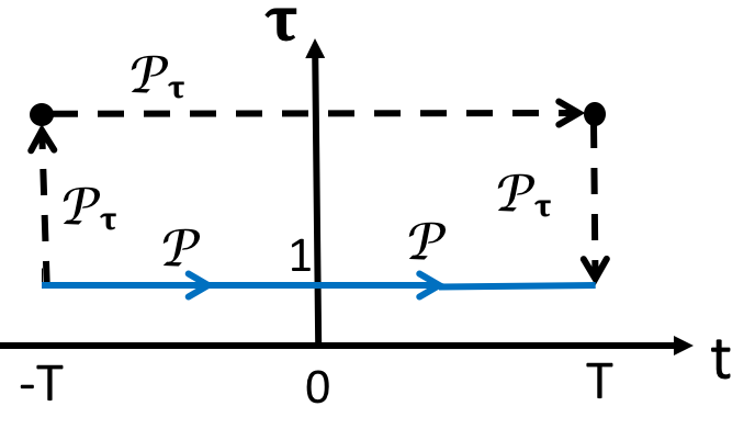
Let the physical evolution correspond to the changes of from to at . Then, starts at the point . We fix, initially, and change from this point to another value, and only then perform -evolution at fixed new . After this, we bring back to at commute; faddeev-book.
The -evolution at fixed or is strictly adiabatic due to the quadratic dependence of the diagonal elements of on . Therefore, the transition probabilities in the LZ-grid models that differ only by within the family (9), which is parametrized by , are identical.
This nontrivial invariance can now be used in combination with a trivial symmetry that is common for all MLZ models. Namely, by rescaling time in the Schrödinger equation (3),
| (14) |
we cannot change the transition probabilities for the evolution in the interval at fixed . On the other hand, this rescaling corresponds to the change of the parameters in the original model (5):
| (15) |
Thus, the transition probabilities are independent of the variable transformations, simultaneously, (9) and (15). Combining them, we find that the transition probabilities in model (5) are invariant of a simple transformation of the diagonal matrices:
| (16) |
This is the most general exact result of our article. The physical meaning of this result is illustrated in Fig. 3. For a model with only two levels in each band in this figure, there are only two independent level splittings
so Eq. (16) means that the transition probabilities depend only on the combination but not on the ratio . It is easy to verify that
has the physical meaning of an area enclosed by the diabatic levels (the diamond plaquette in Fig. 3). Hence, we can also formulate (16) as an invariance of the transition probabilities of the transformations of the LZ-grid that preserve the areas enclosed by the diabatic levels, as well as the LZ parameters if the slopes of the bands are also allowed to change.

Unfortunately, the invariance under the transformations (16) is not sufficient to solve the whole model, i.e., to express the transition probabilities in terms of the known special functions of the model’s parameters. Nevertheless, we will show that this symmetry strongly simplifies the analysis, and even leads to certain further exact relations for the transition probabilities when a model has additional discrete symmetries.
III Quantum dot models
In what follows, we will explore application of the symmetry (16) to two models, which have been studied to some extent for various reasons previously. We will refer to these models as to symmetric and antisymmetric. The symmetric model has the Hamiltonian
| (17) |
and the antisymmetric one has the Hamiltonian
| (18) |
where all parameters are real. The symmetric model has emerged previously in discussions of nonadiabatic behavior in MLZ systems in the large coupling limit malla-LZ.

Physically, both models, (17) and (18), can describe a single electron that jumps between discrete levels of two quantum dots. The linear potential ramp in one of the dots is then induced by applying a time-dependent electric gate voltage difference between the dots, as in the experiments petta-4lz1; petta-4lz2. Each dot has two discrete energy levels. Most naturally, this happens when electronic spin can flip during the tunneling event due to the spin orbit coupling, as shown in Fig. 4.
In the antisymmetric case, with the Hamiltonian , the couplings and describe then the spin preserving and the spin flipping tunneling between the two dots. The minus sign near guarantees the time-reversal invariance of the model. In fact, the Hamiltonian at is the most general, up to gauge transformations, Hamiltonian that one can create for a time-reversed four-state system with spin four-LZ, and the splittings are induced by applying the external magnetic field. Generally, different quantum dots have different g-factors, which then means that .
Both models, and , have elementary discrete symmetries. For example, let
The Hamiltonian has an elementary symmetry
which leads to the symmetry of the evolution operator :
| (19) |
from which follows that the amplitudes and in the symmetric model are purely real. There are also relations between different scattering amplitudes, such as, , , which lead to the relations between the transition probabilities: , , , and . For a reader interested in examples of discrete symmetry effects in other MLZ models, we refer to Refs. four-LZ; li-dynamic.
Similarly, for the antisymmetric model, let
then
from which follows that and are purely imaginary in this model, and there is the same set of relations between the transition probabilities as for the symmetric model.
Apart from this, the transition probability independence of the area conserving transformations (Fig. 3), leads to less intuitive constraints. Namely, since different quantum dots generally have different level splittings, i.e.,
there is generally an asymmetry of dynamics in respect to the initially chosen quantum dot. For example, the trivial symmetry (19) does not predict any relation between the probabilities and , as we illustrate in Fig. 5(a).
However, the invariance of the transition probabilities of the transformations (16) allows us to tune in both models without affecting the transition probabilities. Let us also add the gauge transformation , which does not change the probabilities either. At such values of the parameters, the Hamiltonians (17) and (18) have an additional discrete symmetry. Namely, let
Then, satisfy
from which we obtain additional relations on the transition amplitudes, such as and consequently , e.t.c.. Let us now summarize all the relations among the transition probabilities that follow from simultaneously the integrability and the discrete symmetries of the models. Although the latter symmetries are a bit different for and , they lead to the same relations between the transition probabilities:
| (20) | |||||
| (21) | |||||
| (22) | |||||
| (23) |

While for , the relations (20)-(23) are consequences of trivial discrete symmetries, for they are generally the results of the integrability of the LZ-grid model. We also note that our analysis, and hence relations (20)-(23) apply only to evolution from to , whereas they do not apply to the probabilities at intermediate times, except for , as we illustrate in Fig. 6. Hence, Eqs. (20)-(23) are our first nontrivial prediction for experimental verification.
The integrability of time-dependent Hamiltonians is a type of quantum symmetries that have not been studied experimentally previously. The experiments on Landau-Stückelberg interferometry provide an opportunity to detect the presence of such unusual quantum symmetries by measuring the state-to-state transition probabilities in already available solid state and atomic systems. The deviations from the exact predictions would mean the presence of the terms beyond the standard Hamiltonian , which may emerge either due to nonlinear time-dependence of the gate voltage or effects of the magnetic field on the tunneling amplitudes.
In addition to the integrability conditions, there are six elements of the transition probability matrix that are known exactly and explicitly due to the no-go rule and the Brundobler-Elser formula be; usuki; nogo-LZ. For the antisymmetric model they are
| (24) | |||||
| (25) |
and for the symmetric model we should replace .
In addition to relations (20)-(23), (24), and (25), we can only add the unitarity of the evolution constraints:
It turns out that many of the latter relations are not independent after we include the already mentioned relations. Thus, even having so many constraints, the matrix of the transition probabilities has three unknown independent parameters that have to be calculated separately.
Fortunately, the integrability leads to another simplification of the model’s analysis. Namely, it was shown in quadr-LZ that the integrability enables a semiclassical approach for estimation of the transition probabilities in the nearly-adiabatic limit. It was also noted in quadr-LZ that the analytical formulas that are obtained by this approach often provide a reasonable approximation for the numerical solutions at arbitrary values of the parameters.
Hence, in the following sections we apply this semiclassical approach to our four-state models, and . For simplicity, here we will restrict ourselves only to the transition probability . This transition probability is the most physically interesting, first, because it is the only one that is needed to estimate the probability to remain in the same quantum dot after the time-linear sweep of the gate voltage. Indeed, all the other needed for this probabilities are given by the exact expressions (24) and (25). Moreover, a simple analysis shows that the probability should generally dominate over in the adiabatic limit because the latter become nonzero after two, rather than one in the case of , nonadiabatic overgap transitions.
Second, the transition from level 2 to level 1 is nontrivial even in the limit of large separation of all level crossings because it is then influenced by quantum interference of different evolution trajectories, as we show in Fig. 5(b). The dependence of the probabilities of such transitions on the relative parameter values is understood poorly. Although numerical simulations of few-state systems are easy, they show complex oscillatory behavior on the parameters even in simplest and perturbative regimes kiselev-LZ, so it is hard to see a general pattern for the role of different parameters. Hence, by developing nonperturbative analytical description of in models (17) and (18) we will obtain a useful insight into the interference effects in the nonadiabatic regime.
IV Semiclassical solution for in quantum dot models
In order to find the transition probability for models (17) and (18) in the adiabatic limit, we take advantage of the -independence of the transition probability and make the slopes of the tilted levels, 3 and 4, infinite by setting , as it was done to study the three-state MLZ model in quadr-LZ. The tilted levels cross both the levels 1 and 2 then at time moments:
where “” is for the crossing of level 3 and “” is for the crossing of level 4.
Let us assume that level 3 is initially populated and we want to find the probability to end up on level 4. Following quadr-LZ, we can employ the fact that for high-slope crossing the characteristic time of the nonadiabatic interactions is vanishing as , whereas the nonadiabatic transitions between the diabatic states 3 and 4 take time that is independent of . Hence, we can separately treat the interactions of levels 3 and 4 with level 1, then with each other, and then with level 2. Specific details, however, depend on the models, which we will consider separately.
IV.1 Symmetric model
First, we consider the Hamiltonian in the limit , and where -dependence is according to (9). We introduce the symmetric, , and the anti-symmetric, , combinations of the diabatic states 1 and 2:
| (26) |
As , both levels 3 and 4 couple only to the state and the nonadiabatic transitions to and from happen in the direct vicinity of time moments and . The corresponding coupling is , and the slope difference between the diabatic levels of and either or is . The probabilities of fast transitions from to near and from to near are given by the LZ formula for two state transitions:
In addition, during the time interval the sates and interact with each other, in particular, via the virtual transitions trough and , as explained in quadr-LZ. Hence, the total transition probability from level 3 to level 4 can be expressed via the product of the probabilities
| (27) |
where is the probability to remain in after the dynamics with a effective Hamiltonian that acts in the subspace of during the time interval .
Away from the points , as , the effect of virtual transitions to and from levels 1 and 2 can be calculated perturbatively. Up to the zeroth order in , such transitions lead to an effective Hamiltonian in the subspace of states :
| (28) |
where the index refers to the interactions appearing due to the virtual transitions in the second order of perturbation series over . The higher order corrections due to such transitions in the limit vanish.
The other contribution to the effective two-state Hamiltonian arrives from the splitting of levels 1 and 2, which mixes states :
| (29) |
can be determined by solving the effective Schrödinger equation with the Hamiltonian . After rescaling time , this equation in the basis of states is given by
| (30) |
where
| (31) |
In order to find , we should find the amplitude of evolution from as into as , and take its absolute value squared. Note that the parameter plays the role in (30) of an effective Planck constant.
Thus, the integrability reduces the problem to a two-state system with time-dependent 22 Hamiltonian . It is possible to reformulate equation (30) by changing to the variable , where , and . This makes it standard for application of the, so-called, Dykhne formula for the overgap transition probability between two states approx-LZ5; approx-LZ0 in the adiabatic limit, in which overgap transitions are suppressed exponentially. This formula provides the corresponding slowest decaying exponent and its leading order prefactor. We will use this formula without switching from to because the direct application of the Dykhne formula to the evolution during produces the same final result, and can be equally justified for the evolution (30).
The difference of the eigenvalues of is found analytically:
| (32) |
By equating this difference to zero we find the branching points:
| (33) |
where the square root convention in is chosen so that , and corresponds to the “” sign in (33). Depending on whether the ratio is bigger or smaller than , we found two different types of the behavior.
Phase I: , i.e., . In this case, is real, so the branching points are purely imaginary. The transition probability can be estimated with the standard Dykhne formula as
| (34) |
where the final integration point is the imaginary root in (33) that is closer to the real time axis.
Phase II: , i.e., . Here, the branching points have both real and imaginary parts. Moreover, the imaginary parts are equal to each other, so both the branch cuts are relevant because they correspond to semiclassical evolution trajectories with comparable amplitudes.
The transition probability is given by a generalized Dykhne formula that sums the amplitudes of both trajectories and only then takes its absolute value squared:
| (35) |
where is a geometric phase difference between the two trajectories. It is of subdominant order in comparison to the integrals in (35), and for real Hamiltonians can take only discrete values or . In appendix A, we calculate this phase for both and and show that for the symmetric model .
The integrals in (34), (35) cannot be simplified anymore. In this form, the probability is already much easier to calculate numerically than by solving the Schrödinger equation numerically directly. In appendix B, we show that the integrals can be additionally simplified for some choices of the parameters. Such cases are useful for developing the intuition about the magnitude of and its dependence on the parameters.
The result (35) is valid for . Naturally, at it makes an unphysical prediction: . In order to adjust Eq. (35), we note that in our case
so, we have
and the desired approximation that makes at is
| (36) |
Finally, using (27), we obtain the desired approximation for the four-state model :
| (37) |
In Fig. 7, the analytical predictions (34) and (36) are compared to the results obtained by solving the Schrödinger equation (30) numerically for several values of the parameter combination . The analytical result for the critical case, (the red curve), was taken from appendix Eq. (55). Phases I and II are clearly distinguishable in numerical simulations: in phase I, decays monotonously with increasing , whereas in phase II, oscillates as a function of .
Note also that increases with increasing coupling strength in phase I. For large , the leading contribution to the sum, , is dominated by the transition probability , and consequently . Hence, our result agrees with the asymptotic behavior that was found for the symmetric model in malla-LZ in the limit .
IV.2 Antisymmetric model with the Hamiltonian
For the Hamiltonian (18), there are two couplings, and . The asymmetry between and requires from us to introduce new linear combinations of the states and :
such that couples directly to and couples to . In the limit , both level 3 and level 4 cross the diabatic energies of and at time moments, respectively, and . Hence, the transition probability is
| (38) |
where is the probability of the transition from as to as , and the fast nonadiabatic transitions are given by the standard LZ formula:
In order to find , we follow the previous approach: we rescale time and obtain the analogous to (30) effective Schrödinger equation for evolution in the subspace during time interval and the effective 22 Hamiltonian
| (39) |
where
The corresponding distance between the adiabatic levels of is
| (40) |
This expression has almost the same structure as Eq. (32) for the symmetric model. Similarly, the transition from to requires a passage through the avoided crossing at , and there are two branching points and that are obtained by setting .
However, we found two qualitative differences of the antisymmetric model from the symmetric one. First, the antisymmetric model does not have phase I, i.e., it always leads to the phase with two equally important branch cuts at time points
| (41) |
where the convention for “” is to keep only the square roots in the upper complex plane. Such roots in (41) satisfy the relation as in phase II of the symmetric model. Hence, the antisymmetric model is always in the phase with the oscillatory behavior. Second, we show in appendix A that the geometric phase for the antisymmetric model is . Hence,
| (42) |
In Fig. 8, we provide the numerical check of (42), which confirms the analytical prediction, including the effect of the topological phase .
At , this formula predicts correctly that , and thus does not need further adjustments. However, we found that a slightly better fit to numerical simulations in the strongly nonadiabatic regime for the Hamiltonian is given by
| (43) |
Formulas (37) and (43) become asymptotically exact in the adiabatic limit . It is instructive to look also at how they perform in the strongly nonadiabatic regime, for which they cannot be justified rigorously. In Fig. 9, we show that, although small deviations from the numerically exact predictions are generally visible, in a broad range of the parameters both formulas perform quite well. They still correctly predict multiple oscillations, including phases and amplitudes, even in the nonadiabatic regime. Thus our semiclassical theory is sufficiently rigorous for, e.g., planning the future experiments without resorting to exhaustive numerical simulations.
V Discussion
The concept of integrability in MLZ theory originally was introduced to unify various fully solvable models. Interestingly, there are also large classes of systems that are formally integrable but cannot be fully solved. Thus, we showed that all LZ-grid models satisfy the integrability conditions for time-dependent Hamiltonians commute. As a result, the state-to-state transition probabilities in all such models are invariant of parameter rescaling (16) but this is not sufficient to determine these probabilities analytically.
Nevertheless, this symmetry is nontrivial and different from the set of the previously known exact results that were derived for LZ-grids earlier usuki. In this sense, the integrability commute is akin in effect to a conservation law for a time-independent Hamiltonian.
We are not aware of experimental studies of such symmetries in explicitly time-dependent Hamiltonians, although these symmetries should be realizable in a broad class of physical systems li-dynamic. Given that the Landau-Stückelberg interferometry for a four-state antisymmetric model (18) has been already demonstrated in quantum dots petta-4lz1; petta-4lz2, the integrability of LZ-grids can also be tested. Specifically, for the Hamiltonian (18), we predict nontrivial but simple-looking relations between the state-to-state transition probabilities (20)-(23) in the dynamics induced by a linear potential chirp.
The experiment to observe such a nontrivial symmetry requires a modification of the control and measurement protocol in petta-4lz1. The standard Landau-Stückelberg interferometry protocol induces periodic transitions through the region with nonadiabatic transitions. It leads to spectacular multi-dimensional plots for the state probability dependence on the potential sweeping rate and the duration of the periodic control. However, such measurements are influenced by all parameters of the scattering matrix for a single passage through the nonadiabatic region. Hence, an analytical interpretation of such patterns for multi-state quantum systems is usually problematic due to the large number of relevant parameters.
Here, we propose to explore the multistate Landau-Zener transition probabilities directly, for example, resetting the state and then measuring it after each linear potential chirp in a coupled quantum dot system petta-4lz1. The advantage of such an experiment would be the direct measurement of the characteristics, for which either exact or semiclassical analytical predictions can be established. By comparing the experimental data to the theory, one can then explore such phenomena as the probability oscillations due to completely nonadiabatic interference effects that we exposed, as well as to confirm the exact constraints that follow from the model’s integrablity.
On the side of mathematical physics, we found further confirmations to the conjecture in quadr-LZ that the time-dependent Hamiltonian integrability often leads to a semiclassical approach to calculate the leading contributions to the overgap transition amplitudes in multistate systems. This approach is an opportunity to explore the driven quantum models with considerable complexity. Although generally approximate, it produces reasonable approximations even in the strongly nonadiabatic regime, in which it cannot be rigorously justified.
Our semiclassical analysis reveals that even the simplest driven models can show complex behavior, such as phase transitions, in which the adiabatic limit plays a similar role to the thermodynamic limit in many-body systems. Thus, in the symmetric model, the interfering semiclassical trajectories do not necessarily lead to oscillations of measurable characteristics. Rather there are two phases: one with oscillatory behavior and another one with a monotoneous decay of the transition probability. We also found that models with similar structure and similar oscillatory behavior, can belong to different topological classes that are characterized by the topological phase between the interfering semiclassical trajectories. The integrability allows us to observe and quantify such phenomena in relatively complex and strongly driven quantum systems.
Appendix A Topological -phase
The -phase between the amplitudes of different semiclassical trajectories in complex time has been known in literature, see, e.g., in joye-prefactor. In practice, however, this phase has been usually inferred numerically, and we do not know of a published rigorous analytical theory for its calculation. Therefore, here we provide such a theory, which exposes the topological nature of the -phase and provides a simple path for its calculation. Our models with the Hamiltonians and are particularly suitable for illustration because all calculations for them can be performed analytically, and the results differ for the different models.
The geometric phase appears generally in quantum mechanics when evolution is considered along a closed path in the parameter space. In the context of the Dykhne formula, such a path can be found if we note that the phase difference between the amplitudes of the trajectories, and in Fig. 10(a), that go through two different branching points, is the same as the phase acquired during the evolution along a path , that is, the cyclic trajectory on the Riemann surface that starts and ends at on the original real time axis. follows along its direction marked in Fig. 10(a), and then switches to but follows it in the opposite direction to what is marked in Fig. 10(a). In Fig. 10(b) we show that this path is a knot that winds around the origin points of the branch cuts.
Any real two-state time-dependent Hamiltonian can be written in the form
| (44) |
where , , and are functions of time. Let us then define
| (45) |
Along the cyclic path in complex plane, , an eigenstate of can still be parametrized by an angle :
| (46) |
The topological phase originates from the fact that the Hamiltonian is periodic function of , whereas the eigenstate vector (46) depends on and . Hence, if changes from to during an adiabatic evolution, the Hamiltonian returns to its initial form at the end but the state vector can change sign:
| (47) |
In other words, the state vector acquires a phase . Generally, a periodic adiabatic evolution of parameters changes the angle by , where is an arbitrary integer. The topological phase is then either , if is even, or , if is odd. There cannot be another type of a geometric phase in this case because .
For a closed trajectory , which can be parametrized by time , the topological phase is given by
| (48) |
Note that
For the symmetric model (30), we have
so,
| (49) |
where , and are the two roots in the upper complex half-plane, which are written in (33).
Note that the integrand in (49) has simple poles at rather than the branching points. Hence, the integral over is given by the difference of the residues at these poles, as illustrated in Fig. 10(c):
| (50) |
where is the residue of the expression at a simple pole , and where the minus sign is because winds around and in opposite directions. Substituting the roots from (33) to (50), and making sure that , we find for the effective two-state system with the Hamiltonian that
| (51) |
Analogously, for the effective Hamiltonian (39) that corresponds to the antisymmetric model (18), we have
| (52) |
where are given by (41), and . Substituting (52) and (41) into (50), we find that for the effective Hamiltonian (39) the topological phase is
| (53) |
Thus, despite similar oscillatory behavior, the symmetric and antisymmetric models are characterized by the different values of topological phase . In this sense the models belong to different topological classes.
Appendix B Analytically simple special cases
B.1 Symmetric model: the critical point at
The condition marks the phase transition point between phase I and phase II. In this special case the two branching points are degenerate and purely imaginary, i.e., . The adiabatic energy difference simplifies to
Substituting into the integral in the Dykhne formula (34) we find
Following joye-prefactor, we should set the exponential prefactor in this special case to be 2 rather than 1 because the behavior near the zero is rather than the typical . This leads to the transition probability
| (54) |
This formula is valid only asymptotically in the limit . Without affecting the behavior in this domain, we can also write
| (55) |
which is still generally approximate but has right value, , at . Finally, the semiclassical formula for the transition probability in the original 4-state model for this special case is
| (56) |
B.2 Symmetric model: the case with oscillations at
To calculate the integral, we set
which leads to:
where the analytic expressions for and can be written in terms of the known special functions but the expressions are a bit lengthy. We just give their numerical values, which can be found to very high precision:
The analogous calculation leads to
and then to
which provides the leading exponent for small and is at .
B.3 Antisymmetric model: the case with
In the antisymmetric model there is also a special case
such that the integrals can be computed explicitly. Substituting in (40), we find the eigenvalue difference
and the branch points in the upper half plane are given by
In order to calculate the integral we set
and find
where analytical expressions for and can be written in terms of the known special functions, which can be calculated with high precision. Similarly, we evaluate the integral for the branching point :
Combining the two contributions, and taking into account the topological phase , we finally find:
Acknowledgements
This work was supported by the U.S. Department of Energy, Office of Science, Basic Energy Sciences, Materials Sciences and Engineering Division, Condensed Matter Theory Program. R.K.M. was supported by LANL LDRD program under project number 20190574ECR and Center for Nonlinear Studies under project number 20190495CR.
References
- (1) S. Brundobler, and V. Elser. “S-matrix for generalized Landau-Zener problem”, J. Phys. A 26, 1211 (1993).
- (2) D. A. Harmin and P. N. Price. Incoherent time evolution on a grid of Landau-Zener anticrossings. Phys. Rev. A 49, 1933 (1994).
- (3) D. A. Harmin. Coherent time evolution on a grid of Landau-Zener anticrossings. Phys. Rev. A 56, 232 (1997).
- (4) D. Bouwmeester, I. Marzoli, G. P. Karman, W. Schleich, and J. P. Woerdman. Optical Galton board. Phys. Rev. A 61, 013410 (1999).
- (5) T. Usuki. Theoretical study of Landau-Zener tunneling at the M+N level crossing. Phys. Rev. B 56, 13360 (1997).
- (6) N. A. Sinitsyn and N. Prokof’ev. Nuclear spin bath effects on Landau-Zener transitions in nanomagnets. Phys. Rev. B 67, 134403 (2003)
- (7) K. Saito, M. Wubs, S. Kohler, Y. Kayanuma, and P. Hanggi. Dissipative Landau-Zener transitions of a qubit: bath-specific and universal behavior. Phys. Rev. B 75, 214308 (2007).
- (8) S. Ashhab. Landau-Zener transitions in a two-level system coupled to a finite-temperature harmonic oscillator. Phys. Rev. A 90, 062120 (2014).
- (9) D. A. Garanin, R. Neb, and R. Schilling. Effect of environmental spins on Landau-Zener transitions. Phys. Rev. B 78, 094405 (2008).
- (10) M. Werther, F. Grossmann, Z. Huang, and Y Zhao. Davydov-Ansatz for Landau-Zener-Stueckelberg-Majorana transitions in an environment: Tuning the survival probability via number state excitation. J. Chem. Phys. 150, 234109 (2019).
- (11) F. Bello, N. Kongsuwan, J. F. Donegan, and O. Hess. Controlled Cavity-Free, Single-Photon Emission and Bipartite Entanglement of Near-Field-Excited Quantum Emitters. Nano Lett. 20, 8, 5830 (2020).
- (12) M.Kervinen, J. E. Ramírez-Munoz, A. Valimaa, and M. A. Sillanpaa. Landau-Zener-Stückelberg interference in a multimode electromechanical system in the quantum regime. Phys. Rev. Lett. 123, 240401 (2019).
- (13) Z. Sun, J. Ma, X. Wang, and F. Nori. Photon-assisted Landau-Zener transition: Role of coherent superposition states. Phys. Rev. A 86, 012107 (2012).
- (14) P. Y. Wen, et al.. Landau-Zener-Stückelberg-Majorana interferometry of a superconducting qubit in front of a mirror. Phys. Rev. B 102, 075448 (2020).
- (15) R. K. Malla and M. E. Raikh. Landau-Zener transition in a two-level system coupled to a single highly excited oscillator. Phys. Rev. B 97, 035428 (2018)
- (16) V. N. Ostrovsky, M. V. Volkov, J. P. Hansen, and S. Selsto. Four-state nonstationary models in multistate Landau-Zener theory. Phys. Rev. B 75, 014441 (2007)
- (17) V. A. Yurovsky and A. Ben-Reuven. Curve crossing in linear potential grids: The quasidegeneracy approximation. Phys. Rev. A 63, 043404 – Published 6 March 2001
- (18) N. A. Sinitsyn, and V. Y. Chernyak. The quest for solvable multistate Landau-Zener models. J. Phys. A: Math. Theor. 50, 255203 (2017).
- (19) N. A. Sinitsyn, E. A. Yuzbashyan, V. Y. Chernyak, A. Patra, and C. Sun. Integrable time-dependent quantum Hamiltonians. Phys. Rev. Lett. 120, 190402 (2018).
- (20) V. Y. Chernyak, and N. A. Sinitsyn. Integrability in the multistate Landau-Zener model with time-quadratic commuting operators. arXiv:2006.15144, submitted to J. Phys. A (2021).
- (21) C. Sun, V. Y. Chernyak, A. Piryatinski, and N. A. Sinitsyn. Cooperative Light Emission in the Presence of Strong Inhomogeneous Broadening. Phys. Rev. Lett. 123, 123605 (2019).
- (22) F. Li, V. Y. Chernyak, and N. A. Sinitsyn. Quantum annealing and thermalization: insights from integrability. Phys. Rev. Lett. 121, 190601 (2018).
- (23) V. Y. Chernyak, N. A. Sinitsyn, and C. Sun. Dynamic spin localization and gamma-magnets. Phys. Rev. B 100, 224304 (2019).
- (24) E. A. Yuzbashyan. Integrable time-dependent Hamiltonians, solvable Landau-Zener models and Gaudin magnets. Ann. Phys. 392, 323 (2018).
- (25) Although the LZ formula should be credited to four authors: Landau, Majorana, Zener, and Stückelberg, the interference of semiclassical trajectories, in the context of nonadiabatic transitions, was discussed only by Landau and Stückelberg.
- (26) F. Ginzel, A. R. Mills, J. R. Petta, G. Burkard. Spin shuttling in a silicon double quantum dot. Phys. Rev. B 102, 195418 (2020).
- (27) X. Mi, S. Kohler, and J. R. Petta. Landau-Zener interferometry of valley-orbit states in Si/SiGe double quantum dots. Phys. Rev. B 98, 161404(R)(2018).
- (28) L. D. Faddeev, and L. A. Takhtajan. Hamiltonian Methods in the Theory of Solitons. (Springer, 1987).
- (29) A. Patra, and E. Yuzbashyan. Quantum integrability in the multistate Landau-Zener problem. J. Phys. A 48, 245303 (2015).
- (30) R. K. Malla, and M. E. Raikh. Loss of adiabaticity with increasing tunneling gap in nonintegrable multistate Landau-Zener models. Phys. Rev. B 96, 115437 (2017).
- (31) N. A. Sinitsyn. Solvable four-state Landau-Zener model of two interacting qubits with path interference. Phys. Rev. B 92, 205431 (2015).
- (32) F. Li, and N. A. Sinitsyn. Dynamic Symmetries and Quantum Nonadiabatic Transitions. Chem. Phys. 481, 28 (2016).
- (33) N. A. Sinitsyn. Counterintuitive transitions in the multistate Landau-Zener problem with linear level crossings. J. Phys. A: Math. Gen. 37 10691 (2004).
- (34) M. N. Kiselev, K. Kikoin, and M. B. Kenmoe. SU(3) Landau-Zener interferometry. EPL 104 57004 (2013).
- (35) K. Fukushima, and T. Shimazaki. Lefschetz-thimble inspired analysis of the Dykhne-Davis-Pechukas method and an application for the Schwinger Mechanism. Ann. Phys. 415, 168111 (2020).
- (36) J.‐T. Hwang, and P. Pechukas. The adiabatic theorem in the complex plane and the semiclassical calculation of nonadiabatic transition amplitudes. J. Chem. Phys. 67, 4640 (1977).
- (37) A. Joye. Non-trivial prefactors in adiabatic transition probabilities induced by high-order complex degeneracies. J. Phys. A.: Math. Gen. 26 6517 (1993).