Pattern formation, localized and running pulsation on active spherical membranes
Abstract
Active force generation by actin-myosin cortex coupled to the cell membrane allows the cell to deform, respond to the environment, and mediate cell motility and division. Several membrane-bound activator proteins move along it and couple to the membrane curvature. Besides, they can act as nucleating sites for the growth of filamentous actin. Actin polymerization can generate a local outward push on the membrane. Inward pull from the contractile actomyosin cortex can propagate along the membrane via actin filaments. We use coupled evolution of fields to perform linear stability analysis and numerical calculations. As activity overcomes the stabilizing factors such as surface tension and bending rigidity, the spherical membrane shows instability towards pattern formation, localized pulsation, and running pulsation between poles. We present our results in terms of phase diagrams and evolutions of the coupled fields. They have relevance for living cells and can be verified in experiments on artificial cell-like constructs.
I Introduction
The cell’s ability to change its shape is crucial for many of its functions, e.g., cell motility and division Alberts2009. The associated membrane deformations involve several physical forces Kozlov2016. For example, coupling of local membrane curvature to protein domains, such as the BAR-domain proteins, can sculpt membrane shapes Mills2004; McMahon2005. This mechanism alone can generate supramolecular organization of membrane-associated proteins, as has been shown recently for coccal bacteria S. aureus Garcia-Lara2015; Agudo-Canalejo2017. In eukaryotes, actin polymerization is stimulated locally on the membrane by molecular complexes like Arp2/3 complex and WASP family activators Pantaloni2001; Doherty2008. The inward growth of F-actins, with a rate controlled by cofilin and profilin, can generate active outward push on the membrane Marcy2004; Kuhn2005; Gov2006. The Arp2/3 branching agents generate a dynamic actin network beneath the cell membrane. The myosin-mediated contractility in the cytoskeleton can propagate to the membrane via this network Medeiros2006; Doherty2008; Murrell2015. In a highly branched part of the actin network such an active pull can affect a relatively wider region of the membrane, in contrast, when the filaments are bundled the myosin pull transmits to highly localized parts of the membrane Svitkina2003. The same actin network can generate both pushing and pulling forces on the membrane. Membrane ruffles and traveling waves on cell membranes are ubiquitous in many cell types Allard2012; Ryan2012; Dobereiner2006. The organization of proteins and lipids in multicomponent membranes, formation of membrane domains, and their interaction with the underlying cytoskeleton play important functional role in cell biology Julicher1993; Julicher1996; Sankararaman2002; Hu2011; Banerjee2018; Mayor2004; Jacobson2007. The theoretical description of active surfaces and their application in cell membranes, organelles, and epithelial tissues have seen significant advancement in recent years Salbreux2017a; Morris2019; Mietke2019b; Mietke2019a; Maitra2014; Ramakrishnan2014b; Ramakrishnan2015a; Loubet2012; Turlier2019; Sadhu2019; Sadhu2018. The combination of curvature sensing proteins and transverse active forces due to membrane pumps or cytoskeleton showed possibilities of instability and traveling waves on open flat membranes Prost1998; Ramaswamy2000; Shlomovitz2007; Veksler2007; Shlomovitz2008; Chen2009a; Gov2009; Alaoui2009; Risler2015; Duclut2019. On the other hand, on closed membranes, the emergent features can depend on the superposition of deformation modes.
In this paper, we consider active shape deformations of spherical membranes in the presence of curvature sensing activator proteins (AP) and the cytoskeleton. Many of the immune system cells, including lymphocytes, neutrophils, basophils, are naturally spherical. With the loss of cell adhesion and near cell division, isolated cells adopt a spherical shape Stewart2011. They can maintain their volume by osmotic control and display surface tension regulation Morris2001a. In the bottom-up synthetic biology approach, cell-sized vesicles, liposomes, and emulsion droplets encapsulating cytoskeletal extracts and other proteins can constitute simple models of artificial cells Simon2019; Durre2018; Litschel2018a; Bashirzadeh2019; Tsai2011; Carvalho2013; Keber2014; Fanalista2019; Litschel2021; Litschel2021a; Liu2009a. Equilibrium properties of spherical membranes with volume constraints are controlled by their surface tension and bending rigidity Canham1970; Helfrich1973; Seifert1997. We consider membrane-cortex adhesion Alert2015; Agudo-Canalejo2017 that can be mediated by several ligand and receptor molecules, like Talin and ERM proteins Tsujioka2012; Tsukita1999. The adhesion strength depends on the molecular type and concentration of the ligands and receptors Alert2015. The passive coupling of APs with local membrane curvature preferring hills or valleys can bring APs together to deform the membrane Ramaswamy2000. In addition, the active push due to actin polymerization supports hill formation. The contractile pull by motor proteins from within the cytoskeleton can generate local valleys. In this paper, we explore the resultant coupled dynamics using linear stability analysis and numerical calculations.
Depending on control parameters, the system shows three different non-equilibrium phases, characterized by instability towards pattern formation, localized pulsation, and running pulsation. The spontaneous localization of valley-forming APs coupled with a cytoskeletal pull can lead to a deep inward deformation. Reduction of stabilizing properties like surface tension can assist such membrane instabilities. The competition between hill and valley forming activities coupled to a feedback mechanism and phase lag in the dynamics can induce pulsation on the membrane. Depending on parameter values, we observe traveling pulsation similar to that in open and flat membranes. On a closed membrane, in contrast, counter-propagating waves can superpose to form standing waves. We find such localized pulsations on the spherical membrane over a broad parameter range. A living cell may exploit these properties in producing intended cell shapes, e.g., during cell migration and cell division. On the other hand, the mechanisms we study can be incorporated into artificial cells, making our predictions amenable to direct experimental verifications.
In Sec. II, we present the continuum model for the membrane coupled to APs, the impact of non-equilibrium processes, and the differential equations describing the coupled dynamics. In Sec. III, we first perform linear stability analysis to demonstrate instability and the presence of unstable spirals. We further differentiate the formation of localized and running pulsations and the associated membrane deformations using particular examples. Finally, in Sec. IV, we conclude by presenting a discussion and outlook.
II Model
We consider deformations of a spherical fluid membrane coupled to activator proteins (AP), driven by growing actin filaments and a contractile cytoskeleton. The membrane’s mechanical properties are characterized by surface tension, bending rigidity, and membrane-cortex adhesion. In addition, an osmotic regulation can maintain the cell volume. The APs diffuse on the membrane, deforming the membrane and localizing depending on the membrane curvature. Moreover, they act as nucleation sites of actin filaments that polymerize inwards to generate local outward push on the membrane. In addition, the F-actins are pulled inward actively by the cortical layer of the cytoskeleton.
II.1 Equilibrium description of the membrane and APs
The bending energy of the membrane can be expressed in terms of the Canham-Helfrich free energy Canham1970; Helfrich1973
where, denotes the local mean curvature, is the spontaneous curvature of the undeformed sphere, and denotes the area element. Here is the bending rigidity of the membrane. Here we neglect the Gaussian curvature term. In a multicomponent vesicle it does not impact the vesicle morphology when different membrane patches have the same Gaussian curvature modulus Julicher1993; Julicher1996; Hu2011. Further, we restrict ourselves to deformations that do not change the overall topology.
We consider a membrane area reservoir maintaining a finite surface tension leading to an energy cost
We assume the membrane to be tethered to a rigid cell cortex via an effective spring constant per unit area Alert2015; Agudo-Canalejo2017. The strength of depends on possible direct coupling of the membrane and cortex via proteins, or non-specific interactions like steric repulsion, van der Waals attraction or electrostatic interactions.
The local concentration of APs changes the bending energy cost by (Appendix-A)
where, denotes the AP concentration per unit area, is the inverse compressibility, and the coupling constant controls whether the APs promote and prefer local hill () or valley () on the membrane (see Fig.1() ). A deformed spherical membrane along with its coupling to various force generators are indicated in Fig.1(). The cell can regulate its volume, e.g., by pumping fluid in and out. We use a volume constraint such that . The total number of membrane-bound APs is assumed to be constant . In the following, we describe each of these terms in further detail.
The small relative deformations around an unperturbed sphere of radius , describes the coordinates on the deformed sphere in the spherical polar coordinates. Keeping up to quadratic order in , the bending energy can be expressed as (Appendix B)
| (1) |
integrated over the solid angle . We use two-dimensional gradient and Laplace-Beltrami operator on the unit sphere (Appendix B).
The change in area element is . The volume constraint within quadratic order in gives the relation . Using this we can rewrite . Thus the stretching energy term
| (2) |
The energy cost due to tethering of the membrane to the actomyosin cortex Alert2015; Agudo-Canalejo2017 can be expressed in terms of a harmonic potential
| (3) |
where, denotes an effective spring constant per unit area. Its value increases with the density and spring constant of bound linkers between the membrane and cortex Alert2015 (Fig.1() ).
Keeping up to bilinear order in and , and using , the free energy contributions from APs can be expressed as
| (4) |
The total free energy of the coupled fields of the membrane deforming activator proteins and the deformation is
| (5) |
This describes the equilibrium morphologies of spherical membranes Agudo-Canalejo2017 and in the limit of large reproduces known results for flat membranes Ramaswamy2000 (see Appendix-C).
II.2 Active forces
In addition to the equilibrium forces, actin polymerization from APs against the cortex, with a polymerization rate , generates a reaction force pushing the membrane along the local outward normal (Fig.1() ). Thus corresponds to a force imbalance causing deformation of the membrane. In addition, the inward growing actin filaments experience active inward pull with a rate due to the contractile activity of actomyosin Doherty2008; Medeiros2006 via attached myosin of density . This force propagates to the membrane via the actin network (Fig.1() ). We model this using a spread function. In a highly branched network the myosin pull can affect a relatively wider region of the membrane. However, when the filaments are bundled, it transmits to highly localized parts of the membrane Svitkina2003. It is reasonable to assume that the maximum of such force on the membrane would be located at the same orientational location as the site of force generation in the cortex. We use a Gaussian propagator in the spherical polar coordinates
| (6) |
where parameterizes the angular spread over which the active contractile force gets distributed. Note that in the limit of , the completeness condition of spherical harmonics makes the Greens function absolutely localized in orientation. The resultant contraction on the membrane is . Thus, the total rate of deformation due to activity is given by,
| (7) |

II.3 Coupled dynamics
The non-conservative dynamics of the membrane can be expressed as , where is a thermal noise obeying , . In the absence of active forces, these dynamics lead to equilibrium fluctuations. The evolution of the displacement field within linear order of , and fields have the form
| (8) | |||||
We assume that the number of APs on the membrane is conserved. Its dynamics can be expressed as where is a transport coefficient describing the angular mobility of APs, and the stochastic noise obeys the relations , . Performing the functional differentiation and keeping terms up to linear order
| (9) |
with angular diffusion constant . The cortical myosin undergoes turnover between a passive detached state to an active cross-linked state in which it can pull the actin filament grown from the APs inward. The variation of myosin density can be described by where denotes thermal noise in the myosin on-off rate Shlomovitz2007. In writing this equation, is used as a proxy to the availability of F-actin grown from the APs. The attachment rate of myosin to F-actin is diffusion-limited, and is assumed to be constant. The detachment rate may increase with local load as where sets the scale of detachment force. The elastic load force due to membrane deformation . Thus up to linear order, we replace by , to get
| (10) |
At steady state with being the average concentration of APs. In the following we consider small deviations , and around , and .
III Results
We expand the fields of small deviations in the basis of the spherical harmonics with amplitudes , , and (see Appendix-D and E). Within the mean-field approximation, ignoring stochastic noise, the equations (8), (9) and (10) lead to the dimensionless form,
| (11) |
where , , , , , , , , and . The volume constraint within quadratic order in gives the relation . In terms of spherical harmonics this leads to , i.e., is a term of quadratic order in . Similarly, the constraint on AP number leads to , i.e., is of quadratic order in and bilinear order in and . As a result, and are negligible in linear order. We use and . At the steady state requires .
In the following, we perform a stability analysis of Eq.(11) to determine the dynamical phase behaviors depending on the various control parameters.
III.1 Stability analysis and dynamical phases
We can determine the evolution of the vector analyzing the properties of the stability matrix governing the evolution in Eq.(11), . The stability matrix is a function of alone, as a result, the evolution of is independent of . The eigenvalues can be determined from the characteristic equation
| (12) |
where , with denoting elements of the matrix , and . A summation over repeated indices is assumed. The detailed expressions for the components of , and , , are listed in Appendix-F.
As can be seen from these expressions always, while and can change sign. The possible dynamical phases in the - plane can be determined in terms of the three roots of the cubic polynomial obeying the condition . For , one of the roots remains real negative (positive), if (). The other two roots could be either real negative, or appear as complex conjugate pairs. The dynamics corresponding to all real negative (or at least one positive) roots is linearly stable (unstable). On the other hand, the dynamics displays stable spiral (unstable spiral) behavior if the real part of the complex conjugate solutions, when they are present, is negative (positive). These conditions can be directly verified by noting that in terms of the solutions , the coefficients must obey , and .
The above-mentioned dynamical phases and phase- boundaries in the - plane are illustrated in Fig.2 using a fixed . In the first quadrant, , a phase boundary between the linearly stable () and linearly unstable () phases appears at
| (13) |
In the regime of , another phase boundary between the linearly stable () to stable spiral () phase appears at
| (14) |
Both these phases are stable in the long time limit. The same equation, however, describes a more interesting phase boundary between the linearly unstable () and the unstable spiral () phase, for . Finally, the boundary between the stable spiral () and unstable spiral () phase is described by
| (15) |
The instabilities determine the shape deformations 11 1 The diagonalization of via the similarity transformation can be used to obtain the time-dependent solution in terms of the stochastic noise. Writing , noise and , Eq.(11) leads to providing solution . The existence of instabilities quickly starts to dominate. . Further details of the determination of these phase boundaries are described in Appendix-G. The growing instabilities within linearized analysis are expected to get saturated at late times due to the non-linearities in the system, e.g., associated with bending energy and surface energy costs (Appendix-B). As a result they can lead to pattern formation in phase and limit cycle oscillations in the phase Strogatz2014; cross_greenside_2009.
In the following, using the generalized phase diagram obtained in the - plane, we explore the specific dynamical phase transitions by varying , , and , keeping all other parameters fixed at biologically realizable values (Table-1). The volume constraint ensures the absence of spherically symmetric expansion or compaction corresponding to the mode. As we show in Appendix-H the possible deformations due to mode is always stable. The morphological changes involve only the higher - modes.
| Bending modulus | Shlomovitz2007 | |
|---|---|---|
| Attachment rate | Shlomovitz2007; Chen2009a | |
| Bare detachment rate | Shlomovitz2007 | |
| Angular spread of myosin force | ||
| AP induced curvature | Shlomovitz2007 | |
| AP mobility coefficient | , | |
| Tether |
III.2 Pulsatory deformations
We first consider a negative coupling between AP and membrane curvature, such that APs prefer and induce local hills on the membrane. In Fig. 3()–() we show phase diagrams identifying various behaviors in the small limit. The obtained phase behaviors are due to the competition between active forces , and passive stabilizing factor . The parameters here maintain the relations and , with the transition lines denoted by , where . The system remains in the -phase for , and transits to phase for . The function varies non-monotonically with a maximum at (Fig. 11 in Appendix-I) displaying the presence of a band of corresponding to the phase, such that the system is stable () for all other -values. The deformations displayed in the -phase thus depend on which of the -modes are excited in the system. Setting gives an estimate of the phase boundary, above (below) which all -modes are stable () in figure () and () (figure () ). This is shown by the beaded line denoted by in Fig.3()–(). However, is an integer and not a real number, as a result making this estimate only approximate. The regions shaded orange in Fig.3 denote the phase. Due to the presence of unstable bands, the different regions in Fig.3 correspond to - phase associated with (), (), (), (), and () modes.
The existence of an unstable band gets reflected in the dependence of eigenvalues . We show this in Fig.4 using and , keeping all other parameter values the same as in Fig.3(). Fig.4() shows for all . On the other hand are real negative for (Fig.4() ), while they show complex conjugate values for . Fig.4() shows that the real parts of only for and 4, supporting a narrow band of instability in phase. For they become negative, and the system gets into phase. The imaginary part of shown in Fig.4() determines the frequency of oscillations.


Fig. 3 predicts the onset of - phase corresponding to different -modes. Moreover, the detailed numerical analysis show two different natures of the phase, characterized by spatially localized pulsation and running pulsation. The boundary between these two kinds of pulsations lies in between open symbols and filled (filled ) for () mode. We present their detailed characterization, in the following.

III.2.1 Localized pulsations
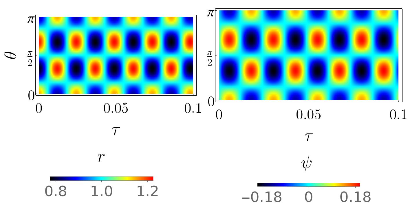
In Fig. 5 we show membrane deformations along with AP localization corresponding to region () of Fig. 3(), using particularly , . The fact that these deformations correspond to localized pulsation is easier to see in the kymographs of and in Fig.(6) plotted at a fixed . The localized pulsations in and appear with a small time-lag, as it takes time for APs to accumulate or disperse and to deform the membrane. Time evolution of mode and corresponding kymograph corresponding to , and of Fig.3(), are shown in Fig.s 2 and 3 of ESI.
The physical mechanism behind the localized pulsation can be ascribed to the following competition. The membrane-AP coupling and the actin polymerization support formation of local outward deformation, while the myosin contractility propagating to membrane via the actin network pulls the membrane inward. It is worthwhile to note that the outward membrane deformation due to AP accumulation is controlled by the membrane-AP coupling and the bending rigidity of the membrane. The small -modes (large wavelength) of membrane deformation takes longer to change. The outward deformations of the membrane accumulates more APs, deforming the membrane further. The time-scale for such accumulation is controlled by the membrane-AP coupling, the bending rigidity, and the mobility of the APs. The outward push due to the actin polymerization reinforces such hill formation. On the other hand, the actomyosin contractility mediated by the spread function pulls the membrane inward. As a result, the hill turns into a valley, and the APs start to move out to neighboring locations with a time-lag controlled by the AP-mobility, the membrane-AP coupling and the membrane bending rigidity. This allows the membrane to relax locally towards the spherical shape, as a new hill starts to appear in the neighborhood. The cycle repeats to sustain oscillations. The specific -mode that is excited controls the shape of the deformation associated with the localized pulsations. In regions () and () in Fig. 3 only one -mode excites behavior controlling the localized pulsations of the sphere. The phase space regions near them are dominated by these -modes. In the presence of localized pulsations, the dynamics on closed membrane differs qualitatively from the open flat membranes that cannot support such standing waves but only show traveling waves of membrane protrusions Shlomovitz2007; Gov2018.
III.2.2 Running pulsations
A remarkable modification of the pulsatory dynamics appears when two modes of similar amplitudes and nearby frequencies are excited together on the closed membrane. For example, we consider the phase-point and of Fig. 3( ) where both and modes are excited together in the -phase. As a result, a running pulsation appears, which can be seen clearly in the kymograph Fig. 7 to run from pole to pole in a to-and-fro motion. The evolution of the deformations on the sphere is shown in Fig. 12 of Appendix-J and movie run_puls.avi in the ESI. As can be seen clearly from the movie, the pole to pole deformations running on the sphere lead to its forward and backward somersaults with time.

The physical mechanism leading to running pulsation is equivalent to that of localized pulsation, in the feedback control and phase lag. The main difference is that here two - modes of similar amplitudes and nearby frequencies are excited together, and they superpose. As a result, the hills and valleys are formed in a connected manner, in both space and time, allowing the deformations to continuously flow over the membrane surface giving rise to a traveling wave. The small difference in their wavelength () and frequency () maintains a traveling wave packet, whose velocity in the flat membrane limit is given by . Lateral waves on cell membranes of various cell types, including mouse embryonic fibroblasts, T-cells, and wing disk cells of the fruit fly, were observed in experiments Dobereiner2006. Localized and running pulsation behaviors have recently been reported for the artificial system of giant unilamellar vesicles encapsulating Min protein system Litschel2018a.
III.3 Pattern formation
Apart from pulsation, Fig. 2 allows the formation of steady patterns, characterized by linear instability. Here we consider a positive membrane- AP coupling , such that APs prefer and induce local valleys on the spherical membrane. Other parameters are fixed at , and (see Table-1). In Fig. 8, we explore deformations as a function of surface tension and the rate of contractile pull . Within the parameter-range explored in this figure . The transition from stable -phase () to linearly unstable -phase () is determined by the condition . Here varies non-monotonically with showing a minimum at . If the value at minimum , this mode and possibly a band of modes around it obeying can show linear instability towards pattern formation. The resultant deformations of the sphere are controlled by this unstable band. In addition, the condition provides a phase boundary independent of , indicated by the dash-dotted line denoted by in Fig. 8, such that the region above this line corresponding to larger surface tension is stable for all -modes. Instability appears only below this line. The lines for a constant in Fig. 8 denote the phase boundaries for particular -modes, with regions above (below) such lines denoting stable (unstable) phase corresponding to the mode. The crossing of different lines shows how instability for -modes shifts from one to another.
The APs prefer to accumulate at valleys. The F-actins grown from the APs are pulled inward more strongly at larger . This bends the membrane further inward recruiting more APs, a positive feedback mechanism that induces linear instability. This mechanism of pattern formation is reminiscent of the pump- bump- clump mechanism described in Ref. 37. The initial progression of deformation at , is shown in Fig. 9. At this parameter value, the modes dominate and determine the observed deformations. Similar deformations, more so for (Fig.7 in ESI), are observed during cytokinesis in cell division Palani2017. The onset of instability can be seen from the kymograph Fig. 10. The high AP density region is associated with inward contraction characterized by small , and vice-versa. As expected, deformations at smaller are easier to set in, and instability appears at smaller values of pulling rate . In Fig. 1 of ESI, we show a phase diagram due to the competition between and for a fixed , displaying transitions between - and -phases.


IV Discussion
In summary, we have discussed active deformations of a spherical membrane adhered to a cell cortex. The membrane is described by its surface tension, bending rigidity, and volume constraint – the shapes of membrane-associated APs couple to the local membrane curvature. We particularly analyzed the impact of active forces due to actin polymerization and the contractile actomyosin cortex on the membrane deformation. The large-scale deformation of the spherical membrane and the dynamic pattern formation of AP concentration is studied using linear stability analysis and numerical calculations.
The generic phase diagram shows possibilities of a stable, unstable, stable spiral, and unstable spiral phases. A closer investigation within a biologically accessible parameter regime revealed localized and traveling pulsation in the unstable spiral phase and pattern formation due to linear instability. The pulsatory patterns are maintained by a negative feedback mechanism between membrane deformation and AP accumulation. We find localized pulsation in the spherical membrane over a broad region of phase space, unlike flat membranes. Further, the spherical membrane shows traveling pulsations running between the poles in a to-and-fro motion at parameter values that excite more than one spherical harmonics of similar amplitudes and nearby frequencies to superpose. A positive feedback mechanism between membrane deformation and AP accumulation, on the other hand, leads to linear instability. However, the amplitudes of growing instabilities found within the linear stability analysis can get saturated by the stabilizing non-linearities arising from the surface and bending energy costs Strogatz2014; cross_greenside_2009.
Using an expansion in the basis of spherical harmonics, we focussed on the small -modes corresponding to large scale deformations. Some insight into the relative role of different terms governing the coupled dynamics in Eq.(11) can be gained by assuming a fast relaxation for APs and myosin concentrations. Setting we get . Further, gives . Using these relations in the first equation of Eq.(11) one can express the slow evolution of the membrane as
The effective bending modulus changes to due to the membrane-AP coupling . The active forces lead to an effective surface tension , where the active tension is
| (16) |
For , increases with the non-local contractile activity , and decreases with the actin polymerization term . Their role reverses with changing sign of the coupling . Such mechanisms can be used by the cell to regulate the membrane tension.
While our analysis incorporating the coupled dynamics of membrane shape, membrane-bound proteins, and active force generators has implications for living cells, our predictions are amenable to direct experimental verification in synthetic cell-like constructs. For example, the different aspects of unstable spiral phase can be tested using an artificial cell. Depending on the known physical parameters one can obtain quantitative estimates from our model. The viscosity of cytoplasmic extract is mPa-s Valentine2005. The F-actin polymerization rate depends on actin concentration. For concentrations up to 4M, the F-actin polymerization rate can vary from 2-20 subunits/s Kuhn2005. Using the subunit size nm, this translates into a growth velocity between 5.52 nm/s and 82.8 nm/s . For a cell of radius m this leads to s-1, which is equivalent to the dimensionless parameter range . The velocity of F-actin moving on myosin depends on ATP concentration, and the particular type of motor protein within the myosin family. The skeletal F-actin moving on muscle myosin can have velocities up to m/s Kron1986 at large ATP concentrations of mM. On the other hand, Myosin XI can have velocities up to m/s Tominaga2003, which is equivalent to the dimensionless parameter . The membrane-cortex adhesion depends on the ligand and receptor molecules mediating it and their concentrations Alert2015. We considered a weak tethering strength pN/m3 describing the adhesion. Reduction of the membrane tension by deflating it using hyper-osmotic shock Simon2019, or incorporating cholesterol Biswas2019 can assist in its easy deformation to build instabilities. The phase diagram in Fig. 3() at corresponds to a surface tension pN/m. At , one expects to find localized pulsations at and running wave for . The predicted oscillations of an artificial cell of radius m will have an amplitude m and a period s. At the above-mentioned parameter range, the active tension (using Eq.(16) with ) shows a times increase with respect to , and corresponds to , a value within the range of measured effective surface tensions in living cells Salbreux2012.
Appendix A Membrane energetics
Assume a flat membrane in the presence of APs that modifies the local intrinsic curvature and bending stiffness. The APs with an area fraction induces a spontaneous curvature , and changes bending rigidity to , such that at places where and where . The modified bending energy of a flat membrane Shlomovitz2008,
For a spherical membrane with intrinsic curvature , replacing by where is the local mean curvature, the expression modifies to
In the last line we kept terms up to bilinear order in curvature and AP concentration. This essentially means retaining only the change in spontaneous curvature due to AP concentration in the energy cost, and neglecting the impact of change in bending rigidity. In the main text we use , and .
Appendix B Quadratic expansion of bending energy
Let n denotes the normal to the surface defined by . The sum of principal curvatures is proportional to the three-dimensional divergence of the normal to the surface, , where the expression of the unit normal is,
where , , are the unit vectors in the , , directions respectively. The total bending energy is therefore expressed as Helfrich1986,
where,
| (17) |
with the radial component of the normal . In the above relations denotes the two-dimensional gradient on the surface of a sphere and denotes the corresponding Laplace-Beltrami operator, given by
Using the above equations we can express the total bending energy in terms of the function where denotes a solid angle. Retaining terms up to second order in
| (18) | |||||
with .
Appendix C Equilibrium fluctuations and the flat membrane limit
At equilibrium using , from Eq.(5), one obtains
| (19) |
denoting non-uniform distribution of coupled with membrane deformation. At equilibrium, mean deformation and mean AP concentration . To explore fluctuations, we expand the fields into spherical harmonics (with , dropping term due to the volume-constraint as shown in the main text, and ) such that , , and use the eigenvalue equation . Using Eq.(19) in the expression of free energy Eq.(5), and , one can write
| (20) |
where . Eq.(20) determines the equilibrium fluctuations through the equipartition theorem. The expression denotes the equilibrium deformation of the membrane due to the membrane-bound activator proteins. The corresponding non-uniform protein distribution is described by , which is obtained by using Eq.(19). The associated pattern formation in the presence of a finite correlation length for density fluctuations of APs has captured supramolecular organization on the membrane of spherical bacteria Staphylococcus aureus Garcia-Lara2015; Agudo-Canalejo2017.
In the limit of large one obtains the flat membrane limit by replacing with , where denotes the wave number corresponding to a mode Loubet2012. The above expression simplifies by using to give,
| (21) |
with a reduction of effective bending rigidity , in agreement with flat membrane result in Ref. 37.
Appendix D Actin-myosin pull
The Greens function is given by . Here we find the result of the integral . We use the expansion of . Using the orthonormality condition , we obtain
| (22) |
Appendix E Linearized dynamics
Expanding the relative deformations , AP concentration , and myosin concentration in spherical harmonics with amplitudes , and , respectively, the coupled linear differential equations describing the dynamics can be expressed as
| (23) | |||||
| (24) | |||||
| (25) |
where we used , and the fact that the Laplace-Beltrami operator is diagonal in the basis of spherical harmonics . In deriving the above relations, we used , , , . The last term on the right hand side of Eq.(23) involving , appears after performing the integration . Plugging in the expression of the Greens function , along with the expansion in the integral, and using the orthonormality condition , one obtains
| (26) |
Appendix F Stability matrix
The elements of are given by , , , , , where . The linear stability of the system is determined by the nature of the eigenvalues of . The eigenvalue equation . The mathematical expressions of the coefficients are
Appendix G Linear stability analysis involving a cubic polynomial
Here we present the details of calculating the generic phase diagram in Fig. 2. We rewrite Eq.(12) as
| (28) | |||||
| (29) |
Intersections between Eq.(28) and Eq.(29) give real roots of Eq.(12). Eq.(28) is a cubic polynomial passing through the origin in - plane. As has been shown in Eq.() . The cubic polynomial can have one minimum at and one maximum at with . Eq.(29) denotes a straight line parallel to axis.
Eq.() shows that although , and can change sign. We can construct a generalized stability diagram in - plane as their signs hold the key to the properties of Eq.(28) and Eq.(29) leading to various possible combinations of roots of Eq.(12), determining the nature of stability. The roots come in the following combinations: () give rise to a linearly stable () phase where the perturbation exponentially decays with time. The two cases () and and () and correspond to linearly unstable () phase as small perturbations grow exponentially with time. The case () and , with real , denotes a (un-)stable spiral () phase if () as the amplitude of oscillation decays (grows) with time. Let us define . The factor theorem gives leading to , , and .
The boundary between linearly stable () and unstable () phase: A transition from - to -phase takes place when among the three negative real roots one changes sign and becomes positive. The condition for the -phase is satisfied when both . The instability appears (-phase) if any one of the roots turns positive requiring . Thus the phase boundary between the - to -phase is given by,
| (30) |
The function depends on and Eq.(30) denotes an - to -transition for a specific - mode. The general condition for the onset of instability can be identified by setting the minimum of to zero. Minimizing , using the discretized condition numerically, we obtain an estimate of , to identify the -independent phase boundary by setting .
The boundary between linearly stable () and stable spiral () phases: A transition from - to -phase happens when the line in Eq.(29) touches the minimum of the polynomial Eq.(28) in the negative side of the axis in - plane making the complex conjugate roots to be real and degenerate at . As we compare the coefficients of the function with , , and we end up with equations,
where is always negative. In the -phase all eigenvalues are negative. Thus all coefficients are positive. Solving the first two equations for and using it in the last equation, we obtain the phase boundary between - and -phase as,
| (31) |
with .
The boundary between stable spiral () and unstable spiral () phase: The unstable spiral () phase is characterized by and . The - to -transition takes place when changes sign. Consequently, the phase boundary is at leading to . Comparing the coefficients, , and with we get conditions that read as,
These conditions lead us to the equation of the phase boundary,
| (32) |
As , the above condition requires both and , therefore the - phase boundary lies in the first quadrant of Fig.2.
The shape fluctuation is determined by the superposition of all unstable modes. The behavior is controlled by . In the presence of a small non-zero real part of , we can write , i.e., . For -modes giving corresponding to the system shows -phase. On the other hand, () corresponds to -phase. The phase boundary, as shown above, is at . For a system in which varies non-monotonically with displaying a maximum, a band of -modes obeying shows - behavior. This happens for parameter values, e.g., in Fig. 3. In such a case, one can maximize using the discretized condition to find . The condition gives the phase boundary between and phase, above which all -modes are stable.
The boundary between unstable spiral () and unstable () phase: The transition between and a linearly unstable phase requires , as this transition, is possible only if the minimum of the cubic polynomial lies at a positive value (note that for ). The instability appears as the minimum of the polynomial in Eq.(28) crosses Eq.(29). At that point, the two degenerate roots become real positive while is still real negative. The positive roots make the perturbation grow in time exponentially and the system becomes linearly unstable.
The boundary between and phase in second quadrant of Fig.2 can be calculated as we did for - to -transition in the first quadrant and end up with the same mathematical expression as in Eq.(31), but now with . Eq.(32) and Eq.(31) meet at origin and this is the only point, where a direct transition from phase in the first quadrant to -phase in the second quadrant possible.
Appendix H Stability of the mode
For mode one can calculate the coefficients of the eigenvalue equation and get
| (33) |
These coefficients are always positive, limiting all the eigenvalues to be either real negative, or one real negative, and a pair of complex conjugates eigenvalues with a negative real part. Consequently, mode is either linearly stable or would show a decaying oscillation in time and thus eliminating any possibility of instability or pattern formation.
Appendix I Transition from to
In Fig. 11 we show the variation of the function as a function of , at three sets of parameter values (), keeping all other parameter values same as in Fig. 3(. All of them show a non-monotonic variation. The range of -values for which shows behavior depends on the dynamical parameters. Fig. 11 shows behavior for mode at , and for mode at . For the parameter combination , both the modes show as for both of them.
Appendix J Running pulsation
In Fig.12 we show changes in the spherical shape as a pulsation runs between the two poles of the sphere. Associated with such deformations, as the movie run_puls.avi in the ESI shows, the spherical membrane performs forward and backward somersaults with time.

Author contributions
DC designed the study with help from S Gutti. S Ghosh performed the linear stability analysis, numerical calculations, and data analysis under the supervision of DC. DC wrote the paper with assistance from S Ghosh.
Conflicts of interest
There are no conflicts to declare.
Acknowledgments
We thank Gijsje Koenderink and Bidisha Sinha for valuable discussions and Thomas Litschel for bringing several relevant experiments to our notice. D.C. thanks SERB, India for financial support through grant number MTR/2019/000750, and International Centre for Theoretical Sciences for an associateship. SG acknowledges Debsuvra Ghosh for help with plots, and thanks QuantiXLie Centre of Excellence, a project co-financed by the Croatian Government and European Union through the European Regional Development Fund - the Competitiveness and Cohesion Operational Programme (Grant No. KK.01.1.1.01.0004).
References
- (1) B. Alberts, D. Bray, K. Hopkin, A. Johnson, J. Lewis, K. R. Martin Raff, and P. Walter, Essential Cell Biology, 3rd ed. (Garland Science, New York, 2009).
- (2) M. M. Kozlov, W. Weissenhorn, and P. Bassereau, in Lecture Notes of the Les Houches School of Physics, edited by E. Pebay-Peyroula, H. Nury, F. Pacy, R. W. H. Ruigrok, C. Ziegler, and L. F. Cugliandolo (Oxford University Press, Oxford, 2016), Chap. Membrane remodeling: theoretical principles, structures of protein scaffolds and forces involved, p. 287.
- (3) I. G. Mills, Y. Vallis, P. J. C. Butler, P. R. Evans, H. T. McMahon, B. J. Peter, and H. M. Kent, Science 303, 495 (2004).
- (4) H. T. McMahon and J. L. Gallop, Nature 438, 590 (2005).
- (5) J. García-Lara, F. Weihs, X. Ma, L. Walker, R. R. Chaudhuri, J. Kasturiarachchi, H. Crossley, R. Golestanian, and S. J. Foster, Proc. Natl. Acad. Sci. U. S. A. 112, 15725 (2015).
- (6) J. Agudo-Canalejo and R. Golestanian, New Journal of Physics 19, 125013 (2017).
- (7) D. Pantaloni, C. Le Clainche, and M. F. Carlier, Science (80-. ). 292, 1502 (2001).
- (8) G. J. Doherty and H. T. McMahon, Annual Review of Biophysics 37, 65 (2008).
- (9) Y. Marcy, J. Prost, M. F. Carlier, and C. Syke, Proc. Natl. Acad. Sci. U. S. A. 101, 5992 (2004).
- (10) J. R. Kuhn and T. D. Pollard, Biophys. J. 88, 1387 (2005).
- (11) N. S. Gov and A. Gopinathan, Biophys. J. 90, 454 (2006).
- (12) N. A. Medeiros, D. T. Burnette, and P. Forscher, Nature Cell Biology 8, 215 (2006).
- (13) M. Murrell, P. W. Oakes, M. Lenz, and M. L. Gardel, Nature Reviews Molecular Cell Biology 16, 486 (2015).
- (14) T. M. Svitkina, E. A. Bulanova, O. Y. Chaga, D. M. Vignjevic, S. ichiro Kojima, J. M. Vasiliev, and G. G. Borisy, J. Cell Biol. 160, 409 (2003).
- (15) J. Allard and A. Mogilner, Curr. Opin. Cell Biol. 25, 107 (2013).
- (16) G. L. Ryan, N. Watanabe, and D. Vavylonis, Cytoskeleton 69, 195 (2012).
- (17) H. G. Döbereiner, B. J. Dubin-Thaler, J. M. Hofman, H. S. Xenias, T. N. Sims, G. Giannone, M. L. Dustin, C. H. Wiggins, and M. P. Sheetz, Physical Review Letters 97, 10 (2006).
- (18) F. Jülicher and R. Lipowsky, Phys. Rev. Lett. 70, 2964 (1993).
- (19) F. Jülicher and R. Lipowsky, Phys. Rev. E 53, 2670 (1996).
- (20) S. Sankararaman, G. I. Menon, and P. B. Sunil Kumar, Phys. Rev. E 66, 031914 (2002).
- (21) J. Hu, T. Weikl, and R. Lipowsky, Soft Matter 7, 6092 (2011).
- (22) T. Banerjee and A. Basu, New J. Phys. 20, 13028 (2018).
- (23) S. Mayor and M. Rao, Traffic 5, 231 (2004).
- (24) K. Jacobson, O. G. Mouritsen, and R. G. Anderson, Nat Cell Biol 9, 7 (2007).
- (25) G. Salbreux and F. Jülicher, Phys. Rev. E 96, 032404 (2017).
- (26) R. G. Morris and M. Rao, Phys. Rev. E 100, 022413 (2019).
- (27) A. Mietke, F. Jülicher, and I. F. Sbalzarini, Proc. Natl. Acad. Sci. 116, 29 (2019).
- (28) A. Mietke, V. Jemseena, K. V. Kumar, I. F. Sbalzarini, and F. Jülicher, Phys. Rev. Lett. 123, 188101 (2019).
- (29) A. Maitra, P. Srivastava, M. Rao, and S. Ramaswamy, Phys. Rev. Lett. 112, 258101 (2014).
- (30) N. Ramakrishnan, P. B. Sunil Kumar, and R. Radhakrishnan, Phys. Rep. 543, 1 (2014).
- (31) N. Ramakrishnan, J. H. Ipsen, M. Rao, and P. B. S. Kumar, Soft Matter 11, 2387 (2015).
- (32) B. Loubet, U. Seifert, and M. A. Lomholt, Phys. Rev. E 85, 031913 (2012).
- (33) H. Turlier and T. Betz, Annu. Rev. Condens. Matter Phys. 10, 213 (2019).
- (34) R. K. Sadhu and S. Chatterjee, Phys. Rev. E 100, 020401 (2019).
- (35) R. K. Sadhu and S. Chatterjee, Phys. Rev. E 97, 032408 (2018).
- (36) J. Prost, J.-B. Manneville, and R. Bruinsma, Eur. Phys. J. B 1, 465 (1998).
- (37) S. Ramaswamy, J. Toner, and J. Prost, Phys. Rev. Lett. 84, 3494 (2000).
- (38) R. Shlomovitz and N. S. Gov, Phys. Rev. Lett. 98, 168103 (2007).
- (39) A. Veksler and N. S. Gov, Biophysical Journal 93, 3798 (2007).
- (40) R. Shlomovitz and N. S. Gov, EPL (Europhysics Lett.) 84, 58008 (2008).
- (41) C. H. Chen, F. C. Tsai, C. C. Wang, and C. H. Lee, Phys. Rev. Lett. 103, 238101 (2009).
- (42) N. S. Gov, Soft Matter 5, 2431 (2009).
- (43) M. D. E. A. Faris, D. Lacoste, J. Pécréaux, J.-F. Joanny, J. Prost, and P. Bassereau, Phys. Rev. Lett. 102, 038102 (2009).
- (44) T. Risler, A. Peilloux, and J. Prost, Phys. Rev. Lett. 115, 258104 (2015).
- (45) C. Duclut, N. Sarkar, J. Prost, and F. Jülicher, Proceedings of the National Academy of Sciences 116, 19264 (2019).
- (46) M. P. Stewart, J. Helenius, Y. Toyoda, S. P. Ramanathan, D. J. Muller, and A. A. Hyman, Nature 469, 226 (2011).
- (47) C. E. Morris and U. Homann, J. Membr. Biol. 179, 79 (2001).
- (48) C. Simon, R. Kusters, V. Caorsi, A. Allard, M. Abou-Ghali, J. Manzi, A. Di Cicco, D. Lévy, M. Lenz, J. F. Joanny, C. Campillo, J. Plastino, P. Sens, and C. Sykes, Nat. Phys. 15, 602 (2019).
- (49) K. Dürre, F. C. Keber, P. Bleicher, F. Brauns, C. J. Cyron, J. Faix, and A. R. Bausch, Nat. Commun. 9, 1630 (2018).
- (50) T. Litschel, B. Ramm, R. Maas, M. Heymann, and P. Schwille, Angew. Chemie - Int. Ed. 57, 16286 (2018).
- (51) Y. Bashirzadeh and A. P. Liu, Soft Matter 15, 8425 (2019).
- (52) F. C. Tsai, B. Stuhrmann, and G. H. Koenderink, Langmuir 27, 10061 (2011).
- (53) K. Carvalho, F.-C. Tsai, E. Lees, R. Voituriez, G. H. Koenderink, and C. Sykes, Proceedings of the National Academy of Sciences 110, 16456 (2013).
- (54) F. C. Keber, E. Loiseau, T. Sanchez, S. J. DeCamp, L. Giomi, M. J. Bowick, M. C. Marchetti, Z. Dogic, and A. R. Bausch, Science (80-. ). 345, 1135 (2014).
- (55) F. Fanalista, A. Birnie, R. Maan, F. Burla, K. Charles, G. Pawlik, S. Deshpande, G. H. Koenderink, M. Dogterom, and C. Dekker, ACS Nano 13, 5439 (2019).
- (56) T. Litschel, C. F. Kelley, D. Holz, M. Adeli Koudehi, S. K. Vogel, L. Burbaum, N. Mizuno, D. Vavylonis, and P. Schwille, Nat. Commun. 12, 2254 (2021).
- (57) T. Litschel and P. Schwille, Annu. Rev. Biophys. 50, 525 (2021).
- (58) A. P. Liu and D. A. Fletcher, Nat. Rev. Mol. Cell Biol. 10, 644 (2009).
- (59) P. B. Canham, J Theor Biol. 26, 61 (1970).
- (60) W. Helfrich, Z. Naturforsch C. 28, 693 (1973).
- (61) U. Seifert, Adv. Phys. 46, 13 (1997).
- (62) R. Alert, J. Casademunt, J. Brugués, and P. Sens, Biophys. J. 108, 1878 (2015).
- (63) M. Tsujioka, S. Yumura, K. Inouye, H. Patel, M. Ueda, and S. Yonemura, Proceedings of the National Academy of Sciences 109, 12992 (2012).
- (64) S. Tsukita and S. Yonemura, J. Biol. Chem. 274, 34507 (1999).
- (65) S. Strogatz, Nonlinear Dynamics and Chaos: With Applications to Physics, Biology, Chemistry, and Engineering, Studies in Nonlinearity (Westview press, Boulder, CO 80301, USA, 2014).
- (66) M. Cross and H. Greenside, Pattern Formation and Dynamics in Nonequilibrium Systems (Cambridge University Press, New York, USA, 2009).
- (67) N. S. Gov, Philos. Trans. R. Soc. B Biol. Sci. 373, 20170115 (2018).
- (68) S. Palani, T. G. Chew, S. Ramanujam, A. Kamnev, S. Harne, B. Chapa-y Lazo, R. Hogg, M. Sevugan, M. Mishra, P. Gayathri, and M. K. Balasubramanian, Current Biology 27, 751 (2017).
- (69) M. Valentine, Z. Perlman, T. Mitchison, and D. Weitz, Biophys. J. 88, 680 (2005).
- (70) S. J. Kron and J. A. Spudich, Proc. Natl. Acad. Sci. U. S. A. 83, 6272 (1986).
- (71) M. Tominaga, H. Kojima, E. Yokota, H. Orii, R. Nakamori, E. Katayama, M. Anson, T. Shimmen, and K. Oiwa, EMBO J. 22, 1263 (2003).
- (72) A. Biswas, P. Kashyap, S. Datta, T. Sengupta, and B. Sinha, Biophys. J. 116, 1456 (2019).
- (73) G. Salbreux, G. Charras, and E. Paluch, Trends Cell Biol. 22, 536 (2012).
- (74) W. Helfrich, Journal de Physique 47, 321 (1986).
- (75) T. Betz and C. Sykes, Soft Matter 8, 5317 (2012).
- (76) A. G. Clark, K. Dierkes, and E. K. Paluch, Biophys. J. 105, 570 (2013).
Electronic Supplementary Information (ESI) for
“Pattern formation, localized and running pulsation on active spherical membranes”
Additional Phase Diagrams and time evolutions
All the simulations are performed at a fixed bending modulus , attachment rate , detachment rate , and spread parameter of myosin pull . In Fig.1 in this ESI, we explore the impact of changing active parameter and the passive stabilizing factor of surface tension keeping fixed. Due to the positive , clustering of APs pull in the membrane locally. The active reaction due to F-actin polymerization, on the other hand, pushes the membrane outward. The surface tension acts as a stabilizing factor.
Fig. 2 of ESI shows localized pulsation corresponding to the excitation of mode at , corresponding to region () of Fig.3() in the main text. The corresponding kymograph in Fig. 3 of ESI shows the evolution of and along the polar angle at a fixed .
In the main text, we have shown a kymograph of running pulsation at in Fig. 7. In Fig. 4 of ESI, we complement it with the kymograph at corresponding to the same set of parameter values, displaying the connected running pulsations. Along with Fig. 7 of the main text, Fig. 4 shows that the local flux corresponding to the traveling wave depends on the location .


Fig. 5 of ESI shows parametric plots comprising of deformation field and local AP density field corresponding to running pulsation at a fixed set of and locations on top of the sphere. The parameter values are listed in figure caption, and correspond to Fig.7 in the main text. We note the existence of multiple periodicity at different locations, and the difference in amplitude of the oscillations in and at various (,) points.
The -mode dependence of real and imaginary parts of eigenvalues distinguish the nature of stable, linearly unstable, and unstable spiral phases. This is shown in Fig. 6 of ESI, corresponding to the running pulsation at parameter values corresponding to Fig.s 7 and 11 of the main text.
Finally in Fig. 7 of ESI we depict conformational changes due to linear instability corresponding to the phase diagram Fig.8 of the main text, at , , where mode is unstable. The corresponding evolution is qualitatively similar to the deformations of a cell at cytokinesis.


Choice of parameters
The cell can change its size and shape by regulating the osmotic pressure and effective surface tension. The bare surface tension of such membranes can be pN/ Betz2012. This is tunable, e.g., the surface tension can be reduced incorporating more cholesterol in the membrane.
The actin polymerization rate at barbed end is . With changing actin concentration from zero to 4 M it varies between subunit/s Kuhn2005. Considering subunit size nm the actin growth rate gives a velocity 5.52 to 82.8 nm/s. To directly translate it to protrusion of spherical membrane of radius m, the relative growth rate is s-1. A myosin drive of F-actin with velocity m/s Kron1986, leads to .
The viscosity of cytoplasmic extract is mPa-s Valentine2005. the viscous friction coefficient turns out to be N s/m pN-s/m assuming the thickness of actin cortex nm Clark2013. Using the radius of spherical membrane m we get the membrane mobility coefficient .
The two dimensional diffusivity of AP is /s Shlomovitz2007; Chen2009a. Considering a vesicle of radius m this gives the angular diffusivity / s-1. Table-2 gives the list of parameter values used in the numerical calculations in this paper.
| Parameters | Definition | Values | Scaled parameters | Scaled values |
|---|---|---|---|---|
| [s-1] | angular diffusivity | unit | ||
| m] | radius | 10 | unit | |
| ] | membrane mobility | 1.0 | unit | |
| AP induced curvature | Shlomovitz2007 | |||
| ] | AP mobility | , | ||
| [pNm] | bare surface tension | 0 – 2 Betz2012 | 0 – | |
| [ ] | bending modulus | 60 Agudo-Canalejo2017 | 25 | |
| [pN/m3] | tether | 0.001, 0.002 Alert2015 | 1000, 2000 | |
| actin polymerization | 0 – 1 Kuhn2005 | 0 – 100 | ||
| myosin contraction | 0 – 1 ( ) | 0 – 100 | ||
| [] | attachment rate | Shlomovitz2007 | ||
| [] | bare detachment rate | Shlomovitz2007 |
Description of videos
The three video in the ESI depict the time evolution in the three distinct dynamical regimes of the spherical membrane predicted by our model. The consecutive frames in localized pulsation (local_pulse.avi), and the running pulsation (run_puls.avi) are separated by dimensionless time gaps and , respectively. In the main text, snapshots from these movies are depicted in Fig.s 5, 6 and Fig.s 7, 11 respectively. The figure captions mention the values of the parameters used.
On the other hand, the consecutive frames in the movie of pattern formation due to linear instability (pattern.avi) is separated by . The snapshots from this movie and corresponding parameter values are shown in Fig.9 of the main text.
References
- (1) T. Betz and C. Sykes, Soft Matter 8, 5317 (2012).
- (2) A. G. Clark, O. Wartlick, G. Salbreux, and E. K. Paluch, Curr. Biol. 24, R484 (2014).
- (3) G. Salbreux, G. Charras, and E. Paluch, Trends Cell Biol. 22, 536 (2012).
- (4) J. R. Kuhn and T. D. Pollard, Biophys. J. 88, 1387 (2005).
- (5) S. J. Kron and J. A. Spudich, Proc. Natl. Acad. Sci. U. S. A. 83, 6272 (1986).
- (6) M. Valentine, Z. Perlman, T. Mitchison, and D. Weitz, Biophys. J. 88, 680 (2005).
- (7) A. G. Clark, K. Dierkes, and E. K. Paluch, Biophys. J. 105, 570 (2013).
- (8) R. Shlomovitz and N. S. Gov, Phys. Rev. Lett. 98, 168103 (2007).
- (9) C. H. Chen, F. C. Tsai, C. C. Wang, and C. H. Lee, Phys. Rev. Lett. 103, 238101 (2009).
- (10) J. Agudo-Canalejo and R. Golestanian, New Journal of Physics 19, 125013 (2017).
- (11) R. Alert, J. Casademunt, J. Brugués, and P. Sens, Biophys. J. 108, 1878 (2015).