Geomagnetic semblance and dipolar-multipolar transition in top-heavy double-diffusive geodynamo models
Abstract
Convection in the liquid outer core of the Earth is driven by thermal and chemical perturbations. The main purpose of this study is to examine the impact of double-diffusive convection on magnetic field generation by means of three-dimensional global geodynamo models, in the so-called “top-heavy” regime of double-diffusive convection, when both thermal and compositional background gradients are destabilizing. Using a linear eigensolver, we begin by confirming that, compared to the standard single-diffusive configuration, the onset of convection is facilitated by the addition of a second buoyancy source. We next carry out a systematic parameter survey by performing numerical dynamo simulations. We show that a good agreement between simulated magnetic fields and the geomagnetic field can be attained for any partitioning of the convective input power between its thermal and chemical components. On the contrary, the transition between dipole-dominated and multipolar dynamos is found to strongly depend on the nature of the buoyancy forcing. Classical parameters expected to govern this transition, such as the local Rossby number -a proxy of the ratio of inertial to Coriolis forces- or the degree of equatorial symmetry of the flow, fail to capture the dipole breakdown. A scale-dependent analysis of the force balance instead reveals that the transition occurs when the ratio of inertial to Lorentz forces at the dominant length scale reaches , regardless of the partitioning of the buoyancy power. The ratio of integrated kinetic to magnetic energy provides a reasonable proxy of this force ratio. Given that in the Earth’s core, the geodynamo is expected to operate far from the dipole-multipole transition. It hence appears that the occurrence of geomagnetic reversals is unlikely related to dramatic and punctual changes of the amplitude of inertial forces in the Earth’s core, and that another mechanism must be sought.
keywords
Dynamo: theories and simulations – Core – Numerical modelling – Composition and structure of the core – Magnetic field variations through time1 Introduction
The exact composition of Earth’s core remains unclear but it is admitted that it is mainly composed of iron and nickel with a mixture of lighter elements in liquid state, such as silicon or oxygen (see Hirose et al. 2013, for a review). The ongoing crystallization of the inner core releases light elements and latent heat at the inner-core boundary (ICB), while the mantle extracts thermal energy from the outer core at the core-mantle boundary (CMB). This combination of processes is responsible for the joint presence of thermal and chemical inhomogeneities within the outer core.
Convection with two distinct sources of mass anomaly is termed double-diffusive convection (Radko 2013, e.g.). A key physical parameter of double-diffusive convection is the Lewis number , defined as the ratio of the thermal diffusivity to the chemical diffusivity . In the liquid core of terrestrial planets, reaches at least (Loper & Roberts 1981; Li et al. 2000, e.g.).
Under double-diffusive conditions, the increase of the background density with depth does not necessarily imply the stability of the fluid in response to perturbations. As shown in Fig. 1, three configurations can be considered:
- (i)
the salt fingering regime, when the background thermal gradient is stabilizing and the mean compositional gradient is destabilizing;
- (ii)
the semi-convection regime, when is destabilizing and is stabilizing;
- (iii)
the top heavy convection regime (also known as double-buoyant), when both and and are destabilizing.
These three cases correspond to three quadrants in Fig. 1, which is inspired by Ruddick 1983. Note that being located inside one of these three quadrants does not necessarily guarantee that convection occurs, since, for all configurations, the onset does not coincide with the origin of the diagram: a critical contrast in temperature, or composition, or both, is required to trigger convective motions. In addition, this diagram does not account for the influence of background rotation (see Monville et al. 2019, for the impact of rotation on the onset in the salt fingers regime), or a magnetic field, on the onset .
Double-diffusive convection has been extensively studied in physical oceanography (Radko 2013, e.g.), as heat and salinity provide two different sources of buoyancy for seawater, as well as in stellar interiors (Spiegel 1972, e.g.), where the molecular diffusivity of composition is only a tiny fraction of the diffusivity of temperature (e.g. Moll et al. 2016, and references therein). To our knowledge, a limited number of studies have been devoted to the analysis of double-diffusive convection in the context of Earth’s core, or more generally in the context of the metallic core of terrestrial planets. They are listed in Fig. 1, with possibly several occurrences of a given study when several of the aforementioned regimes were considered. It appears that the top-heavy configuration has been investigated the most; this is also the configuration we shall focus on in this work.
Previous studies devoted to the top-heavy regime are listed in the top-right quadrant of Fig. 1, starting with hydrodynamic, non-magnetic studies. Considering the limit for a fluid filling a rapidly-rotating annulus, Busse 2002 theoretically predicted that the addition of chemical buoyancy facilitated the onset of standard thermal convection, in two ways. First by lowering the critical value of the Rayleigh number required to trigger the classical spiralling thermal Rossby waves of size and frequency proportional to and , respectively, where is the non-dimensional Ekman number, being the kinematic viscosity, the rotation rate and the size of the fluid domain. Second, and more importantly, by enabling a second class of instability. The latter is characterized by a much lower onset, independent of , a critical length scale of the order of the size of the fluid domain, and a very small frequency, proportional to . Busse 2002 referred to this class of instability as “nearly steady” (i. e. slow) convection, and he argued that it could facilitate “immensely” convection in Earth’s core, though with several caveats (see Busse 2002, for details). Simitev 2011 pushed the analysis further for various , and stressed that the critical onset curve for convective instability in a rotating annulus forms disconnected regions of instabilities in the parameter space. In particular, the second family of modes (i.e. the slow modes) are stable whenever the compositional gradient is destabilizing. Trümper et al. 2012, Net et al. 2012 and Silva et al. 2019 studied the onset of double-diffusive convection in a spherical shell geometry. In the top-heavy regime with , Trümper et al. 2012 confirmed that the addition of a secondary buoyancy source facilitates the convective onset. Net et al. 2012 showed that the properties of the critical onset mode, such as its drift frequency or its azimuthal wave number, strongly depends on the fractioning between thermal and compositional buoyancy. Using a linear eigensolver, Silva et al. 2019 carried out a systematic survey of the onset of convection in spherical shells for the different double-diffusive regimes. In the top-heavy configuration with , they showed that the convection onset is characterized by an abrupt change between the purely thermal and the purely compositional eigenmodes depending on the relative proportion of the two buoyancy sources. In addition, they demonstrated that the onset mode features the same asymptotic dependence on the Ekman number as classical thermal Rossby waves over the entire top-heavy regime (top-right quadrant of Figure 1), thereby casting some doubt on the likelihood of the occurrence of slow modes.
Trümper et al. 2012 performed a series of non-linear, moderately supercritical, rotating convection calculations at constant , for different proportions of chemical and thermal driving. To that end, they conducted a parameter survey, varying the chemical and thermal Rayleigh numbers, to be defined below, while keeping their sum constant. This way of sampling the parameter space, however, does not guarantee that the total buoyancy input power stays constant. This complicates the interpretation of their results, for instance regarding the influence of compositional and thermal forcings on the convective flow properties.
Let us now turn our attention to the few self-consistent dynamo calculations in the top-heavy regime published to date (marked with a cross in the top-right quadrant of Fig. 1). The first integration was reported by Glatzmaier & Roberts 1996. This calculation was an anelastic, double-diffusive extension of the celebrated Boussinesq simulation of the geodynamo by Glatzmaier & Roberts 1995. Glatzmaier & Roberts 1996 assumed enhanced and equal values of the diffusivities, i.e. . Consequently, that simulation did not exhibit stark differences with the purely thermal convective model, except that the dipole did not reverse over the course of the simulated years. The second numerical investigation of geodynamo models driven by top-heavy convection was conducted by Takahashi 2014. His models were based on the Boussinesq approximation with and relatively large Ekman numbers ( ). In addition, Mather & Simitev 2021 identified a few top-heavy Boussinesq dynamos with and , that used stress-free mechanical boundary conditions and appeared to be close to onset. Top-heavy dynamo simulations were also performed by Manglik et al. 2010 and Takahashi et al. 2019 in the context of modelling Mercury’s dynamo.
Double-diffusive models of the geodynamo are the exception rather than the rule, essentially on the account of Occam’s razor. Efforts carried out in the community since the mid nineteen-nineties have been towards understanding the most salient properties of the geomagnetic field using a minimum number of ingredients (e.g. Wicht & Sanchez 2019, for a review). To that end, the codensity formalism introduced by Braginsky & Roberts 1995 is particularly attractive: it assumes that the molecular values of and can be replaced by a single turbulent transport property. Consequently, the mass anomaly field can be described by a single scalar, termed the codensity, that aggregates the two sources of mass anomaly. This approach has the benefit of (i) removing one degree of freedom and (ii) mitigating the numerical cost by suppressing the scale separation between chemical and thermal fields when . With regard to Fig. 1, this amounts to restricting the diagram to either the vertical or the horizontal straight line.
The codensity formalism was quite successful in reproducing some of the best constrained features of the geomagnetic field and its secular variation (Christensen et al. 2010; Aubert et al. 2013; Schaeffer et al. 2017; Wicht & Sanchez 2019, e.g.). Most geodynamo models actually assume that the diffusivity of the codensity field equals the kinematic viscosity, yielding a Prandtl number of unity. A remarkable property of the geodynamo that remains to be explained satisfactorily from the numerical modelling standpoint, is its ability to reverse its polarity every once in a while, that is to go from a dipole-dominated state to another dipole-dominated state through a transient multipolar state (see e.g. Valet & Fournier 2016, for a recent review of the relevant paleomagnetic data). A possibility is that the geodynamo has been, at least punctually in its history, in a dynamical state that can enable the switch between dipole-dominated and multipolar states to occur. A key question that follows is therefore: what are the physical processes that control the transition between dipole-dominated dynamos and multipolar dynamos? This has been analyzed intensively numerically, starting with the systematic approach of Kutzner & Christensen 2002, who demonstrated that a stronger convective driving led to a dipole breakdown, and that for intermediate values of the forcing, the simulated field could oscillate between dipolar and multipolar states.
Sreenivasan & Jones 2006 showed that an increasing role of inertia (through stronger driving) perturbed the dominant Magneto-Archimedean-Coriolis force balance to the point that it led to a less structured and less dipole-dominated magnetic field. In the same vein, Christensen & Aubert 2006 assumed that the transition is due to a competition between inertia and Coriolis force. They introduced a diagnostic quantity termed the local Rossby number , as a proxy of this force ratio. Here denotes the average flow speed and is an integral measure of the convective flow scale. Based on their ensemble of simulations, Christensen & Aubert 2006 concluded that the breakdown of the dipole occurred above a critical value of about , in what appeared a relatively sharp transition (Christensen 2010, see also). If this reasoning gives a satisfactory account of the numerical dataset, its extrapolation to Earth’s core regime raises questions (Oruba & Dormy 2014, e.g.). Since the geomagnetic dipole reversed in the past, the numerical evidence collected so far (see Wicht & Tilgner 2010, for a review) suggests that the geodynamo could lie close to the transition between dipolar and multipolar states. This implies that could be of the order of for the Earth’s core. Geomagnetic reversals should then reflect the action of a convective feature of scale of about (Davidson 2013; Aubert et al. 2017, see). It is very unlikely that such a small-scale flow could significantly alter a dipole-dominated magnetic field.
According to Soderlund et al. 2012, the breakdown of the dipole is rather due to a decrease of the relative helicity of the flow. In numerical dynamo simulations, coherent helicity favors large-scale poloidal magnetic field through the -effect (Parker 1955, see) at work in convection columns and it therefore contributes actively to the production and the maintenance of dipolar field (Olson et al. 1999, e.g.). Conversely, the dipolar field can promote a more helical flow, with the Lorentz force enhancing the flow along the axis of convection columns, as shown by Sreenivasan & Jones 2011. By measuring the integral force balance for dipolar and multipolar numerical dynamos, Soderlund et al. 2012 noticed that the Coriolis force remained dominant, even in multipolar models. Accordingly, they suggested that, in their models, the modification of the flow structure was rather controlled by a competition of second-order forces, with the ratio of inertia to viscous forces as the parameter controlling the transition.
The role played by viscous effects was further stressed by Oruba & Dormy 2014, who proposed that the transition from dipolar to multipolar dynamos in the numerical dataset was controlled by a triple force balance between Coriolis force, viscosity, and inertia. A local Rossby number constructed using the viscous lengthscale, , as opposed to the integral scale discussed above, carries the same predictive power in separating dipolar from multipolar dynamo models (their Fig. 4). This argument was subsequently refined by Garcia et al. 2017, who included the Prandtl number dependence of the critical convective length scale when defining the local Rossby number. From a mechanistic point of view, Garcia et al. 2017 showed that the dipole breakdown was not necessarily correlated to a decrease of the relative helicity, but rather to a weakening of the equatorial symmetry of the flow. Introducing the proportion of kinetic energy contained in this equatorially symmetric component, they demonstrated that the transition could be satisfactorily explained by a sharp decrease of that quantity when the refined local Rossby number exceeded a value of (their Fig. 3d). This would imply that the transition from a dipolar state to a multipolar state would essentially be a hydrodynamic transition. Discussing the implication of their results for the geodynamo, they clearly stated that the role of inertia was presumably overestimated in the numerical dataset that had been investigated so far, stressing the need for stronger field dynamos, where the magnetic field could possibly have an active role.
The early numerical dataset admittedly contained a majority of dynamos operating at large Ekman numbers, and relatively low magnetic Prandtl number . In the dynamos studied by Soderlund et al. 2012, the convective flow was not dramatically altered by the presence of a self-sustained magnetic field. Since then, a large number of simulations have been published with lower values of and comparatively larger values of (Yadav et al. 2016; Schaeffer et al. 2017; Schwaiger et al. 2019; Menu et al. 2020). For those strong-field dynamos, in the sense of a ratio of bulk magnetic energy to bulk kinetic energy larger than one, the magnetic field has a significant impact on the flow, and on the dipolar-multipolar transition. Menu et al. 2020 reported simulations with a prevailing Lorentz force, that remain dipolar way beyond the supposedly critical value. Given that Earth hosts a strong-field dynamo, it is then worth investigating whether the competition between Lorentz force and inertia may actually lead to the transition.
In order to shed light on this particular issue, and to further strengthen our understanding of double-diffusive dynamos, we have performed a suite of novel dynamo models, comprising , , simulations with top-heavy, purely thermal, purely chemical driving, respectively. The goal of this work is twofold: on the one hand, we will follow an approach similar to that of Takahashi 2014 and study to which extent the relative proportion of chemical to thermal driving impacts the earth-likeness (in a morphological sense) of the simulated magnetic fields. On the other hand, we will examine whether this proportion has an impact on the dipolar to multipolar transition. Takahashi 2014 reported a drop of the dipolarity when the relative contribution of thermal convection to the total input power exceeds . We will analyze whether this was a fortuitous consequence of the cases he considered, and whether we can find a more general rationale to explain the transition, by careful inspection of the force balance at work.
This paper is organized as follows: the derivation of the governing equations and their numerical approximations are presented in Section 2. The results are described in Section 3. We proceed by firstly investigating the onset of convection for top-heavy convection. The impact of the input power distribution on the Earth-likeness is then explored. Finally we examine the transition between dipolar and multipolar dynamos. Section 4 discusses the results and their geophysical implications.
2 Model and methods
2.1 Hypotheses
We operate in spherical coordinates and consider a spherical shell of volume filled with a fluid delimited by the inner core boundary (ICB), located at the radius , on one side and by the core mantle boundary (CMB), located at the radius , on the other side with . The shell rotates about the -axis with a constant rotation rate , where is the unit vector in the direction of rotation. The equation of state
| (1) |
describes how the density of the fluid varies with temperature and composition . In this equation, and are the coefficients of thermal and chemical expansion, , and the average temperature, density and composition of lighter elements in the outer core.
The properties of the fluid, including its kinematic viscosity , its magnetic diffusivity , its specific heat , its chemical and thermal diffusivity (), its coefficients of thermal and chemical expansion (, ) are assumed to be spatially uniform and constant in time. Due to the almost uniform density in the outer core, we also assume a linear variation of the acceleration of gravity with radius. The physical and thermodynamical properties of the Earth’s core relevant for this study are given in Table 4.
| Definition | Symbol | Value | Reference (Lower bound - Upper bound) |
|---|---|---|---|
| Inner radius | Dziewonski & Anderson 1981 | ||
| Outer radius | Dziewonski & Anderson 1981 | ||
| Earth angular velocity | |||
| Gravitational acceleration at CMB | Dziewonski & Anderson 1981 | ||
| Core density at CMB | Dziewonski & Anderson 1981 | ||
| Specific heat | Labrosse 2003 | ||
| Heating power from core | Buffett 2015 | ||
| Thermal conductivity at CMB | Konôpková et al. 2016 - Pozzo et al. 2013; Zhang et al. 2020 | ||
| Thermal diffusivity | () | Estimated using values of , and . | |
| Coefficient of thermal expansion | Labrosse 2003 | ||
| Kinematic viscosity | Roberts & King 2013 | ||
| Magnetic diffusivity | Pozzo et al. 2013 - Konôpková et al. 2016 | ||
| Estimated magnetic field strength | Gillet et al. 2010 | ||
| Superadiabatic composition contrast | 0.02 - 0.053 | Badro et al. 2007 - Anufriev et al. 2005 | |
| Chemical diffusivity | ( – ) | Loper & Roberts 1981 - Li et al. 2000 | |
| Coefficient of chemical expansion | Braginsky & Roberts 1995 - Labrosse 2015 | ||
| Estimated flow velocity | Finlay & Amit 2011 |
| Name | Symbol | Definition | Core | This study |
|---|---|---|---|---|
| Ekman | – | |||
| Thermal Rayleigh | ||||
| Chemical Rayleigh | ||||
| Magnetic Prandtl | 0.5 – 5 | |||
| Thermal Prandtl | – | 0.3 | ||
| Schmidt | – | 3 | ||
| Lewis | – | 10 |
| Name | Symbol | Definition | Core |
|---|---|---|---|
| Typical rotation time | |||
| Turnover time | |||
| Magnetic diffusion time | |||
| Thermal diffusion time | |||
| Viscous diffusion time | |||
| Chemical diffusion time | – |
| Name | Symbol | Definition | Earth’s core | This study | Reference |
|---|---|---|---|---|---|
| Relative thermal convective power | see Eq. 15 | Lister & Buffett 1995 - Takahashi 2014 | |||
| Rossby | Table 4 | ||||
| Local Rossby | Davidson 2013 - Olson & Christensen 2006 | ||||
| Relative equat. symmetric kinetic energy | Aubert et al. 2017 | ||||
| Magnetic Reynolds | Table 4 | ||||
| Elsasser | Table 4 | ||||
| Dipolarity parameter | Gillet et al. 2015 |
2.2 Governing equations
Convection of an electrically-conducting fluid gives rise to a magnetic field . The state of the fluid is then described by the velocity field , the magnetic field , the pressure , the temperature and the composition . The equations governing the dynamics of the flow under the Boussinesq approximation are cast in a non-dimensional form. We adopt the thickness of the shell as reference length scale and the viscous diffusion time as time scale. A velocity scale is then given by . Composition is scaled by , pressure by , power by and magnetic induction by , where is the magnetic permeability of vacuum. Temperature unit is based on the temperature gradient at , , or at , , depending on the thermal boundary conditions. Under the Boussinesq approximation, the equation for the conservation of mass is
| (2) |
The dynamics of the flow is described by the Navier-Stokes equation, expressed in the frame rotating with the mantle
| (3) |
where is the unit vector in the radial direction. The time evolution of the magnetic field under the magnetohydrodynamics approximation is given by the induction equation
| (4) |
Finally, the evolution of entropy and composition are governed by the similar transport equations
| (5) |
and
| (6) |
where is a volumetric internal heating and a chemical volumetric source.
The set of equations (2 – 6) is governed by 6 dimensionless numbers: The Ekman number expresses the ratio between viscous and Coriolis forces
the Prandtl (Schmidt) number between viscous and thermal (chemical) diffusivities
and the magnetic Prandtl number between viscous and magnetic diffusivities
The thermal and chemical Rayleigh numbers
where is the gravitational acceleration at the CMB, measure the vigour of thermal and chemical convection. Note that the Lewis number discussed in the Introduction is the ratio of the Schmidt number to the Prandtl number,
Table 4 provides estimates of these control parameters for the Earth’s core. These nondimensional number express the ratio of characteristic physical time scales
where is the typical rotation time, the viscous diffusion time, the magnetic diffusion time, the thermal diffusion time and the chemical diffusion time.
Earth’s outer core evolves on a broad range of time scales, as one can glean from the inspection of Table 4. In particular, even if the evolution of temperature and composition are governed by similar transport equations (see Eq. 5 and 6), thermal diffusion is much more efficient than chemical diffusion, which causes the Lewis number to greatly exceeds unity (see Tab. 4). This implies that the typical lengthscale of chemical heterogeneities is possibly several orders of magnitude smaller than the length scale of thermal heterogeneities. The values of the control parameters spanned by the simulations presented in this work are discussed in section 2.6.
2.3 Boundary conditions
The inner core is growing and is ejecting light elements because of its crystallization, which in principle yields coupled boundary conditions for temperature and composition (Glatzmaier & Roberts 1996; Anufriev et al. 2005, e.g.). For the sake of simplicity, thermal and chemical boundary conditions are considered as decoupled here, as in e.g. Takahashi 2014. We consider two different setups to explore the impact of varying the thermal boundary conditions:
- (i)
Fixed fluxes: thermal and composition fluxes are imposed at both boundaries with
(7) - (ii)
Hybrid: temperature is fixed at the ICB while the temperature flux is imposed at the CMB, the boundary conditions on chemical composition are the same as in the previous setup
(8)
No-slip mechanical boundary conditions are used at both boundaries. The mantle is assumed to be insulating, such that the magnetic field at the CMB has to match a source-free potential field. The inner core is treated as a rigid electrically-conducting sphere which can freely rotate around the -axis (Hollerbach 2000; Wicht 2002, e.g.). Its rotation is a response to the viscous and magnetic torques exerted by the outer core on the inner core. The conductivity of the inner core is assumed to be equal to that of the outer core, and its moment of inertia is calculated by using the same density as the liquid outer core.
2.4 Numerical approach
We solve the system of equations (2– 6) using the open-source geodynamo code MagIC11 1 https://magic-sph.github.io/ (Wicht 2002; Gastine et al. 2016). This code has been validated against a benchmark for double-diffusive convection initiated by Breuer et al. 2010.
The solenoidal vectors and are decomposed in poloidal and toroidal potentials
where is the radius vector. The new unknowns are then , , , , , and .
Each of these scalar fields is expanded in spherical harmonics to maximum degree and order in the horizontal direction. The spherical harmonic representation of the magnetic poloidal potential reads
where is the coefficient associated to , the spherical harmonic of degree and order . The non-linear terms are calculated in physical space. The open-source SHTns library22 2 https://bitbucket.org/nschaeff/shtns (Schaeffer 2013, see) is used to compute the forward and inverse spectral transforms on the unit-sphere.
In the radial direction, MagIC uses either a finite difference scheme, or a Chebyshev collocation method (Boyd 2001, see). The finite difference grid, whose number of points is denoted by , is regularly spaced in the bulk of the domain, and follows a geometric progression near the boundaries (Dormy et al. 2004, see). When the collocation approach is selected, Chebyshev polynomials are truncated at degree and the collocation points are defined by
| (9) |
Due to the particular choice of spatial grid given by the equation above, the transforms between physical grid and Chebyshev representation are carried out by fast discrete cosine transform (see Press et al. 1992, chapter 12). This discretisation yields a point densification close to the boundaries which could impose severe time step restrictions when the magnetic field is strong (Christensen et al. 1999, see). To mitigate this effect, we adopt the mapping proposed by Kosloff & Tal-Ezer 1993 and replace in Eq. (9) by
where is the mapping coefficient. To maintain the spectral convergence of the simulation has to verify
| (10) |
where is the machine precision.
Figure 2 shows the minimum grid spacing as a function of for a regular grid, the finite difference grid with geometrical clustering near the boundaries, and two collocation grids, with (Gauss-Lobatto grid) and . Because when using the classical Gauss-Lobatto grid, adopting the mapping by Kosloff & Tal-Ezer 1993 yields a possible increase of by a factor when . The time step size could in principle rise by a comparable amount, should it be controlled by the propagation of Alfvén waves in the vicinity of the boundaries (Christensen et al. 1999). Using the finite difference method enables even larger grid spacing and hence possible additional gain in the time step size. This speed-up shall however be mitigated by the fact that has to be increased by a factor to when using finite differences to achieve an accuracy comparable to that of the Chebyshev collocation method (Christensen et al. 2001; Matsui et al. 2016, see).
is then expanded in truncated Chebyshev series
| (11) |
with
where the double primes on the summations indicate that the first and the last indices are multiplied by one half (Glatzmaier 1984, see). In the above equations, is the -th order Chebyshev polynomial at the collocation point defined by
Further details on spherical harmonics and Chebyshev polynomials expansion can be found in Tilgner 1999 and Christensen & Wicht 2015.
Once the spatial discretisation has been specified, the set of equations (2–6) complemented by the boundary conditions (see Eq. 7 and 8) forms a semi-discrete system where only the time discretisation remains to be expressed. As an example, the time evolution of the poloidal potential for the magnetic field (see Eq. 11) can be written as an ordinary differential equation
| (12) |
where is the initial condition, a non linear-function of and and a linear function of . The above equation serves as a canonical example of the treatment of the different contributions: the non-linear terms are treated explicitly (function ) while the remaining linear terms are handled implicitly (function ). In MagIC, several implicit/explicit (IMEX) time schemes are employed to time advance the set of equations (2–6) from to :
- (i)
a combination of a Crank-Nicolson for the implicit terms and a second-order Adams-Bashforth for the explicit terms called CNAB2 (Glatzmaier 1984, see),
- (ii)
two IMEX Runge-Kutta : PC2 (Jameson et al. 1981, see) and BPR353 (Boscarino et al. 2013, see).
CNAB2 has been commonly used in geodynamo models since the pioneering work of Glatzmaier 1984. IMEX Runge-Kutta schemes have been rarely employed in the context of geodynamo models (Glatzmaier & Roberts 1996), rapidly-rotating convection in spherical shells (Marti et al. 2016) or quasi-geostrophic models of 2-D convection (Gastine 2019). For IMEX Runge-Kutta schemes, substages are solved to time-advance Eq. (12) from to
| (13) |
where , is the intermediate solution at substage , and . is then given by
| (14) |
In the above equations, the matrices and and the vectors , , and form the so-called Butcher tables of the IMEX Runge Kutta schemes given in Appendix A. Since the last lines of are equal to for PC2 and BPR353, the last operation to retrieve (Eq. 14) is actually redundant with the last sub-stage (Ascher et al. 1997, see). IMEX Runge-Kutta schemes require more computational operations to time advance the set of equations(2–6) from to than CNAB2. However, they allow larger time step sizes that compensate for this extra numerical cost (Marti et al. 2016) and they are more accurate and stable. Since BPR353 is a third-order scheme, it is particuraly attractive to ensure an accurate equilibration of the most turbulent runs.
2.5 Simulation diagnostics
For each diagnostic quantity , we adopt in the following overbars for time averaging and angle brackets for spatial averaging
where corresponds to the averaging time.
2.5.1 Integral quantities and scales
The magnetic and kinetic energies are given by
where is the inner core volume. By multiplying the Navier-Stokes equation (3) by and the induction equation (4) by , we obtain the following power balance
In the case of double-diffusive convection, the energy is provided by chemical and thermal buoyancy power and defined by
and dissipated by viscous and Ohmic dissipations and given by
Once a statistically steady state has been reached, the input buoyancy powers should compensate the Ohmic and viscous dissipations. Following King et al. 2012, to assess the consistency of the numerical computations, we measure the time-average difference between input and output powers
We made sure that this difference remained lower than for all the simulations reported in this study. This value is below the threshold considered as sufficient to ensure the convergence of integral diagnostics (King et al. 2012; Gastine et al. 2015, see). For each simulation, the total convective power and the relative thermal convective power are defined by
| (15) |
hence vanishes for a purely chemical forcing and is equal to for a purely thermal forcing.
Following Christensen & Aubert 2006 and Schwaiger et al. 2019, we introduce two quantities to characterise the typical flow lengthscale. The integral scale already discussed in the introduction is obtained from the time-averaged kinetic energy spectrum
where is the kinetic energy contained in spherical harmonic degree , while the dominant lengthscale is defined as the peak of the poloidal kinetic energy spectra (Schwaiger et al. 2019; Schwaiger et al. 2021)
where is the contribution of spherical harmonic degree to the total poloidal kinetic energy.
In order to explore the impact of the equatorial symmetry of the flow on the dipole-multipole transition, we consider the relative equatorially-symmetric kinetic energy introduced by Garcia et al. 2017
| (16) |
where is the kinetic energy contained in the non-zonal flow and the kinetic energy contained in the equatorially-symmetric part of the non-zonal flow.
We measure the mean convective flow amplitude either by the magnetic Reynolds number or by the Rossby number defined by
where is the characteristic turnover time and the root mean square flow velocity. Following Christensen & Aubert 2006, we define a local Rossby number by
The dipolar character of the CMB magnetic field is quantified by its dipolar fraction , defined as the ratio of the axisymmetric dipole component to the total field strength at the CMB in spherical harmonics up to degree and order .
Figure 3 shows the statistical distribution of for the simulations reported in this study. Two distinct groups of numerical simulations separated by a gap at are visible in this figure. A magnetic field is considered as dipolar when and multipolar otherwise. This bound differs from the original threshold of considered by Christensen & Aubert 2006, but it is found to better separate the two types of dynamo models contained in our dataset. Note that the same bound of 0.5 was recently chosen by Menu et al. 2020 in their study. The magnetic field amplitude is measured by the Elsasser number
Finally, transports of heat and chemical composition are quantified by using the Nusselt and the Sherwood number defined by (see Goluskin 2016, chapter 1)
where , are the temperature and composition differences between the ICB and the CMB, and the subscript stands for the background conducting state. For both the fixed fluxes and hybrid configurations (recall section 2.3 above), we obtain a background composition contrast given by
| (17) |
where is the radius ratio. The background temperature drop depends on the imposed boundary conditions. For the fixed flux setup, it reads
| (18) |
while it becomes
| (19) |
for the hybrid setup.
Table 4 gives the definition of most of these integral diagnostics and provides estimates for Earth’s core, along with the bracket of values obtained in the numerical dataset presented here.
2.6 Exploration of parameter space
We compute simulations varying the Ekman number, the magnetic Prandtl number, the thermal and the chemical Rayleigh numbers. The properties of this dataset are listed in Tab. 6. The less turbulent simulations have been initialized with a strong dipolar field and a random thermo-chemical perturbation. Their final states have been used as initial conditions for the more turbulent simulations, in order to shorten their transients. Three different Ekman numbers are considered in this study : , and . has been varied between and and between and to study the influence of the convective forcing and span the transition between dipole-dominated and multipolar dynamos. We adopt and (i.e. ) for a better comparison with previous studies (Takahashi 2014, e.g.) and to mitigate the computational cost associated with large Lewis numbers. varies between and , depending on the Ekman number, in order to maintain . The numerical models were integrated for at least 20 % of a magnetic diffusion time for the most turbulent (and demanding) ones, and for more than one for the others, in order to ensure that a statistically steady state had been reached.
3 Results
3.1 Onset of top-heavy convection
Figure 4 shows the location of the computed numerical simulations for the three considered Ekman numbers in the parameter space (, ) defined by
where corresponds to the thermal (chemical) Grasshof number,
Adding to in the above equations allows us to use logarithmic scales in the top row of Fig. 4.
We determine the onset of convection using the open-source software SINGE33 3 https://bitbucket.org/vidalje/singe which computes linear eigenmodes for incompressible, double-diffusive fluids enclosed in a spherical cavity (Schaeffer 2013; Vidal & Schaeffer 2015; Kaplan et al. 2017; Monville et al. 2019, see). For a fixed (), the code solves the generalized eigenvalue problem formed by the linearized Navier-Stokes and transport equations. It seeks eigenmodes of the form
where is a function of and , is the azimuthal wave number and the complex angular frequency. Starting at a specific (, ), the critical mode is determined by varying one of the Rayleigh numbers (keeping the other fixed) in order to obtain an with a vanishing imaginary part. The onset mode is then characterized by its critical chemical and thermal Rayleigh numbers (, ), its critical azimuthal wave number and its (real) angular drift frequency . Connecting the (, ) pairs that we collected with SINGE gives rise to the critical curves plotted in Fig. 4. In each panel, the intersection of these curves with the -axis (resp. -axis) corresponds to the critical Rayleigh number for purely thermal (resp. chemical) convection. Underneath the critical curves, the grey-shaded areas are regions of the parameter space where thermal and chemical perturbations are unable to trigger a convective flow.
We note that the shape delimited by the critical curves in the bottom row of Fig. 4 is not rectangular, as would be the case if the two sources of buoyancy were independent. Instead, we observe a decrease of the critical when increases for the three different Ekman numbers. As previously reported by Busse 2002, Trümper et al. 2012 and Net et al. 2012, and discussed in the Introduction, this demonstrates that the addition of a second buoyancy source facilitates the onset of convection as compared to the single diffusive configurations.
Starting from and following the critical curve for each Ekman number, grows until one reaches the upper right ”corner” of the onset region and then decreases to a value comparable to the starting value when tends to zero. We observe that is nearly constant on the vertical branches, while it increases much faster on the horizontal ones, as already reported by Trümper et al. 2012.
As can be seen in Figs. 4(e) and 4(f), the shaded shape is much wider with fixed-flux boundary conditions than with hybrid boundary conditions. This comes from the difference in the temperature contrasts of the background conducting states. An adequate way to compare both setups resorts to using diagnostic Grasshof numbers
| (20) |
that are based on the temperature (composition) contrasts () of the reference conducting state instead of the control thermal (chemical) Grasshof numbers () (Johnston & Doering 2009; Goluskin 2016, see). Using Eqs. (18) and (19), the temperature difference between ICB and CMB for the conducting states for both setups reads
which is in good agreement with the actual ratio of critical observed in panels (e) and (f) of Fig. 4.

The analysis of the onset of double-diffusive convection becomes even more straightforward if one adopts the formalism introduced by Silva et al. 2019. This framework rests on two parameters: first, the diagnostic effective Grasshof number
| (21) |
and second the Grasshof mixing angle such that
| (22) |
The pair can be interpreted as the polar coordinates of the critical onset mode in the Cartesian parameter space. A mixing angle hence corresponds to purely thermal convection, while corresponds to purely chemical convection. Figure 5 shows the critical effective Grasshof number , the critical azimuthal wave number and the critical angular drift frequency , multiplied in each instance by their expected asymptotic dependence on the Ekman number for purely thermal convection, as a function of the Grasshof mixing angle . Adopting a diagnostic effective Grasshof number conveniently enables the merging of the onset curves associated with the two sets of thermal boundary conditions (fixed-flux and hybrid).
The onset curves can be separated into two branches: (i) From up to , the onset mode almost behaves as a pure low- thermal mode with little change in and a large drift speed; (ii) a sharp transition to another kind of onset mode, reminiscent of the convection onset, is observed for . The latter is characterized by a smaller drift frequency, a higher azimuthal wavenumber and a lower effective Grasshof number . The critical azimuthal wavenumber reaches its maximum for before gradually decreasing to reach a value comparable to that expected for purely thermal convection towards .
The Ekman dependence is almost perfectly captured by the asymptotic scalings and for the critical wavenumber and the drift frequency . The case of mixing angles with constitutes an exception to this rule with a sharp drop to a constant critical wavenumber (see the small kink in the upper left part of Fig. 4d). The dependence of on the Ekman number shows a more pronounced departure from the leading-order asymptotic scaling . As shown by Dormy et al. 2004 for differential heating (see e.g. their Fig. 5), the higher-order terms in the asymptotic expansion of as a function of the Ekman number are still significant for (Schaeffer 2016, see also). Given the range of Ekman numbers considered for this study, it is not suprising that the asymptotic scaling for is not perfectly realized yet.
In summary, the onset of double-diffusive convection in the top-heavy regime takes the form of thermal-like drifting Rossby-waves, the nature of which strongly depends on the fraction between chemical and thermal forcings. This confirms the results previously obtained by Silva et al. 2019 (their Fig. 9).
3.2 A reference case
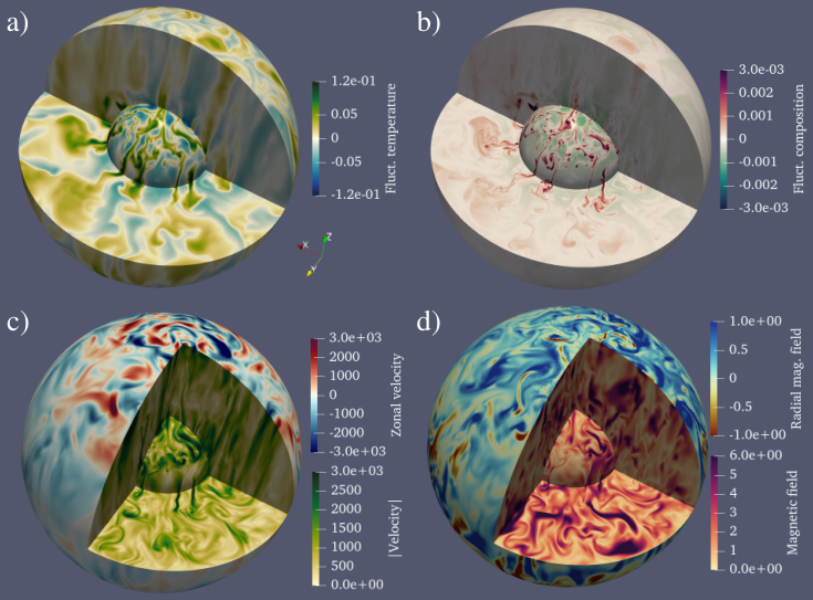

We will now focus on the simulation marked by an asterisk (*) in Table 6 and in Figure 4 to highlight specific double-diffusive convection features. This simulation corresponds to , , and with hybrid boundary conditions. The thermal convective power amounts on average for of the total input power. Since the local Rossby number reaches , this simulation is expected to operate in a parameter regime close to the transition between dipolar and multipolar regimes () put forward by Christensen & Aubert 2006. This high value of also indicates the sizeable role played by inertia in the force balance of this simulation. Figure 7 shows 3-D renderings of several fields extracted from a snapshot taken over the course of the numerical integration: (a) temperature perturbation, (b) composition, (c) zonal velocity and magnitude of the velocity vector, (d) radial magnetic field and magnitude of the magnetic field vector. We chose the radius of the inner and outer spheres of these renderings to place ourselves outside thermal and compositional boundary layers. Convection is primarily driven by the chemical composition flux at the ICB. Because of the contrast in diffusion coefficients (), compositional plumes develop at a much smaller scale than that of thermal plumes (see Fig. 7a and Fig. 7b). Having also induces a chemical boundary layer much thinner than the thermal one, as illustrated by the Sherwood number being five times larger than the Nusselt number in this case (44.8 versus 8.0, see Tab. 6). The emission of a thermal plume is likely triggered by an impinging chemical plume. Accordingly, one would expect temperature fluctuations to be enslaved to compositional fluctuations, which may explain the outstanding spatial correlation between temperature and composition noticeable in Fig. 7(a) and Fig. 7(b). This correlation was already reported by Trümper et al. 2012 for predominantly thermal convection.
In typical dipole-dominated dynamos, the velocity field features extended sheet-like structures that span most of the core volume (Yadav et al. 2013; Schwaiger et al. 2019, see). Because of the strong forcing that characterizes the reference simulation, the convective flow is organised on smaller scales, which likely reflects the sizeable amplitude of inertia. The magnetic field is dominated by its axisymmetric dipolar component (see Fig. 7a), despite the supposed proximity of the simulation with the dipolar-multipolar transition zone. Inspection of Table 6 indicates that this snapshot-based observation can in fact be extended to the entire duration of the simulation (close to half a magnetic diffusion time), as the average dipolar fraction is equal to .
The radial magnetic field features intense localized flux patches of mostly normal polarity in each hemisphere, with a few reverse flux patches paired with normal ones, mostly at high latitudes. Those fluid regions hosting a locally strong magnetic field are characterized by more quiescent flows, as can be seen in the equatorial planes of Fig. 7(c) and Fig. 7(d) in the vicinity of the outer boundary. In a global sense, our reference simulation can be qualified as a strong-field dynamo since the ratio of the magnetic energy to kinetic energy is slightly larger than unity, .
Figure 7 shows a comparison between the radial component of the magnetic field at the CMB (left) and its representation truncated at spherical harmonic degree (right). The truncated field presents several key similarities with the geomagnetic field at the CMB, such as a significant axial dipole and patches of reverse polarity in both hemispheres.
3.3 Earth-likeness
For a more quantitative assessment of the Earth-likeness of the dynamo models, we employ the rating of compliance introduced by Christensen et al. 2010. This quantity is derived from four criteria based on the magnetic field at the CMB truncated at the degree
- (i)
the relative axial dipole energy , which corresponds to the ratio of the magnetic energy in the axial dipole field to that of the rest of the field up to degree and order eight,
- (ii)
the equatorial symmetry corresponding to the ratio of the magnetic energy at the CMB of components that have odd values of for harmonic degrees between two and eight to its counterpart in components with even,
- (iii)
the zonality , which corresponds to the ratio of the zonal to non-zonal magnetic energy for harmonic degrees two to eight at the CMB,
- (iv)
the flux concentration factor , defined by the variance in the squared radial field.
To evaluate these quantities for the Earth, Christensen et al. 2010 used different models based on direct measures such as gufm1 model by Jackson et al. 2000 and IGRF-11 model (Finlay et al. 2010, from), as well as archeomagnetic and lake sediment data (Korte et al. 2005, model CALS7K.2 from) and a statistical model for paleofield (Quidelleur & Courtillot 1996, see). These models allow to estimate the evolution of the mean value of the Gauss coefficients and their variances. Finally, they obtained the values given in Table 5 for the four rating parameters.
| Name | Earth’s value | Simulation (*) |
|---|---|---|
| 1.4 | 2.69 | |
| 1.0 | 1.75 | |
| 0.15 | 0.25 | |
| 1.5 | 1.46 |
These values are used to determine the rating of compliance between numerical dynamo models and the geomagnetic field expressed by
where , Var() is the variance of and the exponent stands for the Earth core. The agreement between simulation and Earth is termed by Christensen et al. 2010 as excellent if , as good when , as marginal wen and non-compliant when . We adopt the same classification in the following. According to Table 5, the relative axial dipole power () and the equatorial symmetry () of the reference simulation (*) are too large in comparison with the reference geomagnetic values, which penalises the overall compliance of the simulation. Nevertheless, the simulation remains in excellent agreement with the geomagnetic field with .
Based on this rating of compliance , Christensen et al. 2010 propose a representation to classify the different numerical dynamos according to the ratio of three different timescales: the rotation period , the advection time and the magnetic diffusion time . Those can be cast into two dimensionless numbers: the magnetic Reynolds number defined by and the magnetic Ekman number defined by . Figure 8 shows our numerical simulations plotted in the parameter space (,). For comparison purposes, the simulations by Christensen et al. 2010 with or (triangular markers) have been added to our dynamo models. To single out the effect of the diffusivities, the purely chemical, the double-diffusive and the purely thermal simulations have been plotted separately. The black symbol marks the approximate position of Earth’s dynamo in this representation (see Tab. 4 and Tab. 4). Christensen et al. 2010 posited the existence, in this parameter space, of a triangular wedge (delimited by dashed lines in Fig. 8), inside which the numerical dynamos yield Earth-like surface magnetic fields (those from our dataset are shown in Fig. 8 with dark blue and blue disks for Excellent and Good ratings, respectively). Below the wedge, weakly super-critical dynamos feature too dipolar magnetic fields, on the account of the modest value of the magnetic Reynolds number. Conversely, a significant increase of the input power at a given yields small-scale convective flows, which possibly lead to the breakdown of the axial dipole (multipolar simulations displayed with crosses in Fig. 8). We observe in Fig. 8 that the upper boundary of the wedge actually depends on the value of : while several purely chemical simulations are already multipolar below , the transition to multipolar dynamos is delayed to for the purely thermal ones. Although all those dynamo models that possess a good or excellent semblance with the geomagnetic field at the CMB lie within the boundaries of the original wedge, having a pair that lies within this wedge cannot be considered as a sufficient condition to produce an Earth-like magnetic field, since the wedge includes a number of simulations with marginal or poor semblance.
To further discuss the impact of on the morphology of the magnetic field at the CMB, Fig. 9 shows in the parameter space (, ) for the three different Ekman numbers considered here. The dashed lines mark the tentative boundaries between dipolar and multipolar simulations in term of . The dipole-multipole transition is delayed to larger input power at lower Ekman numbers. Decreasing indeed enables the exploration of a physical regime with lower prone to sustain dipole-dominated dynamos (Kutzner & Christensen 2002; Christensen & Aubert 2006, see). The input power required to obtain multipolar dynamos is multiplied by roughly when decreasing from to . For each Ekman number, the width of the dipolar window strongly depends on since the actual input power needed to reach the transition is an order of magnitude lower for pure chemical convection than for pure thermal convection. Simulations with are found to behave similarly as purely thermal convection. We further observe that Earth-like dynamos can be obtained for any partitioning of power injection with the best agreement obtained close to the dipole-multipole transition. This is a consequence of the way we have sampled the parameter space, mainly adopting one single value for each Ekman number. Magnetic Reynolds numbers conducive to yield Earth-like fields are then attained at strong convective forcings. Adopting larger values at more moderate chemical and thermal Rayleigh numbers could hence produce Earth-like fields further away from the dipole-multipole transition (Christensen et al. 2010, see). Additional diagnostics are hence required to better understand why the dipole-multipole transition depends so strongly on the nature of the convective forcing.
3.4 Breakdown of the dipole
The physical reasons which cause the breakdown of the dipole in numerical models remain poorly known. Several previous studies suggest that the dipole may collapse when inertia reaches a sizeable contribution in the force balance (Sreenivasan & Jones 2006; Christensen & Aubert 2006, see).
Christensen & Aubert 2006 introduced the local Rossby number as a proxy of the ratio between inertia and Coriolis force and found no dipole-dominated dynamos for (Christensen 2010, see). Figure 10 shows as a function of for the simulations computed in this study. The vertical line marks the threshold value of put forward by Christensen & Aubert 2006, while the horizontal line corresponds to , the boundary between dipolar and multipolar dynamos adopted in this study. To single out the effect of partitioning the input power between chemical and thermal forcings, the symbols have been color coded according to . Each subset of models with comparable exhibits the same decrease of with as reported by Christensen & Aubert 2006. However, the dipole-multipole transition occurs at lower when decreases. For , the transition happens close to while it happens around for . In addition, the dynamo models with are clearly separated in two groups of simulations with either or , while the dipole-multipole transition is much more gradual for pure chemical forcing. hence fails to capture the transition between dipolar and multipolar dynamos, independently of the transport properties of the convecting fluid.
Following Christensen & Aubert 2006, Garcia et al. 2017 also envision that the increasing role of inertia would be responsible for the dipole breakdown. They however define another parameter to characterize it. They suggest that the transition is related to a change in the equatorial symmetry properties of the convective flow. To quantify it, they introduce the ratio previously defined in Eq. (16). Figure 11 shows as a function of . Geophysical estimates for are based on the study of Aubert 2014. The decrease of the relative equatorial symmetry goes along with a gradual weakening of the axisymmetric dipolar field. Below , no dipolar dynamos are obtained while conversely the models with are all dipolar. However, this parameter has little predictive power to separate the dipolar solutions from the multipolar ones over the intermediate range .
Another way to examine the dipole-multipole transition resorts to looking at the force balance governing the outer core flow dynamics (Soderlund et al. 2012; Soderlund et al. 2015, see). To do so, we analyse force balance spectra following Aubert et al. 2017 and Schwaiger et al. 2019. Each force entering the Navier-Stokes equation (3) is hence decomposed into spherical harmonic contributions. The spatial root mean square of a vector reads
| (23) |
where represents the thickness of the viscous boundary layer and the outer core volume that excludes those boundary layers. By using the decomposition in spherical harmonics, the above expression can be rearranged as
We define the time-averaged spectrum as a function of the harmonic degree for the force by the relation
| (24) |
Figure 12 shows the time-averaged force balance spectra for one dipolar and one multipolar dynamo with and . For both panels, the spherical harmonic at which the poloidal kinetic energy peaks is indicated by filled markers.
The left panel corresponds to the force balance of the reference case (*) which is in excellent agreement with the geomagnetic field in terms of its low value (recall Sec.3.2). Its spectra feature a dominant quasi-geostrophic balance between Coriolis and pressure forces up to accompanied by a magnetostrophic balance at smaller scales. The difference between pressure and Coriolis forces, forming the so-called ageostrophic Coriolis force (long dashed line), is then balanced by the two buoyancy sources (short dashed line) at large scales and by Lorentz force (irregular dashed line) at small scales. This forms the quasi-geostrophic Magneto-Archimedean-Coriolis balance (QG-MAC) devised by Davidson 2013 and expected to control the outer core fluid dynamics (Roberts & King 2013, see). This hierarchy of forces is similar to the one observed in geodynamo models that use a codensity approach (Aubert et al. 2017; Schwaiger et al. 2019, e.g.). The breakdown of buoyancy sources reveals a dominant contribution of chemical forcings which grows at small scales. The QG-MAC balance is perturbed by a sizeable inertia, which reaches almost a third of the amplitude of Lorentz force below , while viscous effects are deferred to more than one order of magnitude below. Because of the strong convective forcing, the force separation is hence not as pronounced as in the exemplary dipolar cases by (Schwaiger et al. 2019, their Fig. 2).
By increasing the input power by a factor while keeping constant, we obtain a numerical model (**) (see Tab 6 and Fig. 4c) where dynamo action yields a multipolar field. As compared to the dipole-dominated solution, the amplitude of each contribution is hence shifted to higher values. Most noticeable changes concern the prominent contribution of the chemical buoyancy for the degree and the ratio of inertia to Lorentz force. The former comes from a pronounced equatorial asymmetry of the chemical fluctuations. The development of strong equatorially-asymmetric convective motions has been observed by Landeau & Aubert 2011 and Dietrich & Wicht 2013 with a codensity approach and flux boundary conditions. Below , inertia reaches a comparable amplitude to Lorentz force, while the smaller scales are still controlled by magnetic effects. This differs from the multipolar dynamo model described by Schwaiger et al. 2019, where inertia was significantly larger than Lorentz force at all scales forming the so-called quasi-geostrophic Coriolis-Inertia-Archimedian balance (Gillet & Jones 2006, e.g.). Here the situation differs likely because of the larger , which enables a stronger magnetic field (Menu et al. 2020, see). At the dominant lengthscale , the ratio is around for the multipolar model, while it is less than for the dipolar one. To examine whether the dipole-multipole transition is controlled by the ratio of inertia over Lorentz forces, we hence focus on the force balance at the dominant lengthscale , in contrast to previous studies, which analysed ratio of integrated forces (Soderlund et al. 2012; Soderlund et al. 2015; Yadav et al. 2016).
Figure 13 shows the time-averaged force balance at for the simulations with and . The dynamics at is primarily controlled by the geostrophic balance between the Coriolis force and the pressure gradient. The other contributions grow differently with : viscosity and inertia increase continuously while Lorentz force at hardly increases beyond . The dipole-multipole transition occurs when inertia reaches a comparable amplitude to Lorentz force at (crosses).
The relevance of this force ratio for sustaining the dipolar field has already been put forward by Menu et al. 2020, using models with a purely thermal forcing and . By considering turbulent simulations with large , they show that strong Lorentz forces at large scale prevent the collapse of the dipole by inertia. As a result, they report dipole-dominated simulations with which exceeds the limit of proposed by Christensen & Aubert 2006. Here, we quantify the contribution of inertia at the dominant convective lengthscale by dividing the amplitude of inertia by the amplitude of Coriolis and Lorentz forces.
Figure 15(a) shows our simulations in the parameter space defined by the amplitude ratios (, ). Each simulation is characterized by the proportion of thermal convection and the nature of its thermal boundary conditions. Increasing the input power of the dynamo leads to a growth of inertia, such that the strongly-driven cases all lie in the upper right quadrant of Fig. 15(a). The transition from dipolar to multipolar dynamos occurs sharply when exceeds over a broad range of ranging from to . This indicates that the transition is much more sensitive to the ratio of inertia over Lorentz force than to the ratio of inertia over Coriolis force. The transition for purely chemical simulations (white symbols) is reached at lower values of and is more continuous than for the thermal ones (black symbols). This confirms the trend already observed in Fig. 10, where shows a much more gradual decreases with when .
Figure 15(b) shows as a function of . In contrast with the previous criteria, the ratio successfully captures the transition between dipole-dominated and multipolar dynamos which happens when , independently of the buoyancy power fraction. The simulation, which singles out in the upper right quadrant of Fig. 15(b), is an exception to this criterion. This numerical model corresponds to with , with hybrid boundary conditions. Although it features , its magnetic field is on time-average dominated by an axisymmetric dipole (). This dynamo however strongly varies with time with several drops of the dipolar component below (see Fig. 16 in the appendix). Although the numerical model has been integrated for more than two magnetic diffusion times, the stability of the dipole cannot be granted for certain.
4 Summary and discussion
Convection in the liquid outer core of the Earth is thought to be driven by density perturbations from both thermal and chemical origins. In the vast majority of geodynamo models, the difference between the two buoyancy sources is simply ignored. In planetary interiors with huge Reynolds numbers, diffusion processes associated with molecular diffusivities could indeed possibly be superseded by turbulent eddy diffusion (Braginsky & Roberts 1995, see). This hypothesis forms the backbone of the so-called “codensity” approach which assumes that both thermal and compositional diffusivities are effectively equal. This approach suppresses some dynamical regimes intrinsic to double-diffusive convection (Radko 2013).
The main goal of this study is to examine the impact of double-diffusive convection on the magnetic field generation when both thermal and compositional gradients are destabilizing (Takahashi 2014, the so-called top-heavy regime, see). To do so we have computed global dynamo models, varying the fraction between thermal and compositional buoyancy sources , the Ekman number and the vigor of the convective forcing using a Prandtl number and a Schmidt number . We have explored the influence of the thermal boundary conditions by considering two sets of boundary conditions for temperature and composition.
Using a generalised eigenvalue solver, we have first investigated the onset of thermo-solutal convection. In agreement with previous studies (Busse 2002; Net et al. 2012; Trümper et al. 2012; Silva et al. 2019), we have shown that the incorporation of a destabilizing compositional gradient actually facilitates the onset of convection as compared to the single diffusive configurations by reducing the critical thermal Rayleigh number. The critical onset mode in the top-heavy regime of rotating double-diffusive convection is otherwise similar to classical thermal Rossby waves obtained in purely thermal convection (Busse 1970).
To quantify the Earth-likeness of the magnetic fields produced by the non-linear dynamo models, we have used the rating parameters introduced by Christensen et al. 2010. Using geodynamo models with a codensity approach, Christensen et al. 2010 suggested that the Earth-like dynamo models are located in a wedge-like shape in the 2-D parameter space constructed from the ratio of three typical timescales, namely the rotation rate, the turnover time and the magnetic diffusion time. Here, we have shown that the physical parameters at which the best morphological agreement with the geomagnetic field is attained strongly depend on the ratio of thermal and compositional input power. In particular, we obtain purely-compositional multipolar dynamo models that lie within the wedge region of Earth-like dynamos (recall Figure 8a). This questions the relevance of the regime boundaries proposed by Christensen et al. 2010.
We have then used our set of double-diffusive dynamos to examine the transition between dipolar and multipolar dynamos. We have assessed the robustness of several criteria controlling this transition that had been proposed in previous studies. Sreenivasan & Jones 2006 suggested that the dipole breakdown results from an increasing role played by inertia at strong convective forcings. Christensen & Aubert 2006 then introduced the local Rossby number as a proxy of the ratio of inertial to Coriolis forces. They suggested that marks the boundary between dipole-dominated and multipolar dynamos over a broad range of control parameters. Our numerical dynamo models with follow a similar behaviour, while the transition between dipolar and multipolar dynamos occurs at lower () when chemical forcing prevails. A breakdown of the dipole for dynamo models with was already reported by Garcia et al. 2017 using under the codensity hypothesis (their Fig. 1).
Using non-magnetic numerical models, Garcia et al. 2017 further argued that the breakdown of the dipolar field is correlated with a change in the equatorial symmetry properties of the convective flow. They introduced the relative proportion of kinetic energy contained in the equatorially-symmetric convective flow, , and suggested that multipolar dynamos would be associated with a lower value of this quantity. However, our numerical dataset shows that multipolar and dipolar dynamos coexist over a broad range of (, recall Fig. 11), indicating that this ratio has little predictive power in separating dipolar from multipolar simulations.
While neither nor provide a satisfactory measure to characterise the dipole-multipole transition, the analysis of the force balance governing the dynamo models has been found to be a more promising avenue to decipher the physical processes at stake (Soderlund et al. 2012; Soderlund et al. 2015). By considering a spectral decomposition of the different forces (Aubert et al. 2017; Schwaiger et al. 2019, e.g.), we have shown that the transition between dipolar and multipolar dynamos goes along with an increase of inertia at large scales. The analysis of the force ratio at the dominant scale of convection has revealed that the dipole-multipole transition is much more sensitive to the ratio of inertia to Lorentz force than to the ratio of inertia to Coriolis force. The transition from dipolar to multipolar dynamos robustly happens when the ratio of inertial to magnetic forces at the dominant lengthscale of convection exceeds , independently of and the Ekman number. This confirms the results by Menu et al. 2020 who argued that a strong Lorentz force prevents the demise of the axial dipole, delaying its breakdown beyond (their Figs. 3 and 4).
Providing a geophysical estimate of the ratio of inertial to magnetic forces at the dominant scale of convection in the Earth’s core is not an easy task. Recent work by Schwaiger et al. 2021 suggests that the dominant scale of convection should be that at which the Lorentz force and the buoyancy force, both second-order actors in the force balance, equilibrate. Extrapolation of this finding to Earth’s core yields a scale of approximately km, that corresponds to spherical harmonic degree . This is far beyond what can be constrained through the analysis of the geomagnetic secular variation. Estimating the strength of both Lorentz and inertial forces at that scale is hence out of reach.
We can however try to approximate the ratio of these two forces by a simpler proxy, namely the ratio of the total kinetic energy to total magnetic energy . To examine the validity of this approximation, Fig. 15 shows as a function of the ratio for our numerical simulations complemented with the codensity simulations of Christensen 2010 that have . We observe that the dipolar fraction exhibits a variation similar to that shown in Fig. 15(b) for the actual force ratio. The transition between dipolar and multipolar dynamos is hence adequately captured by the ratio (Kutzner & Christensen 2002). All but one of the numerical dynamos of our dataset become multipolar for , independently of , , and the type of thermal boundary conditions prescribed. Using the physical properties from Tab. 4 leads to the following estimate for the Earth’s core
Christensen 2010 and Wicht & Tilgner 2010 argued that convection in the Earth’s core should operate in the vicinity of the transition between dipolar and multipolar dynamos in order to explain the reversals of the geomagnetic field. This statement, however, postulates that reversals and the dipole breakdown are governed by the same physical mechanism. The smallness of for Earth’s core indicates that it should operate far from the dipole-multipole transition, contrary to the numerical evidence accumulated up to now. The paleomagnetic record indicates that during a reversal or an excursion, the intensity of the field is remarkably low, which suggests that the strength of the geomagnetic field could decrease by about an order of magnitude. This state of affairs admittedly brings the ratio closer to unity, yet without reaching it. So it seems that the occurrence of geomagnetic reversals is not directly related to an increase of the relative amplitude of inertia. Other mechanisms proposed to explain geomagnetic reversals rely on the interaction of a limited number of magnetic modes, whose nonlinear evolution is further subject to random fluctuations (Schmitt et al. 2001; Pétrélis et al. 2009, e.g.). In this useful conceptual framework, the large-scale dynamics of Earth’s magnetic field is governed by the induction equation alone. The origin of the fluctuations that can potentially lead to a reversal of polarity is not explicited and it remains to be found, but evidence from mean fields models by Stefani et al. 2006 suggests that the likelihood of reversals increases with the magnetic Reynolds number. In practice, these fluctuations could very well occur in the vicinity of the convective lengh scale, and have either an hydrodynamic, or a magnetic, or an hydromagnetic origin, depending on the process driving the instability. Shedding light on the origin of these fluctuations constitutes an interesting avenue for future numerical investigations of geomagnetic reversals.
5 Acknowledgments
We would like to thank Ulrich Christensen and Julien Aubert for sharing their data. Numerical computations were performed at S-CAPAD, IPGP and using HPC resources from GENCI-CINES and TGCC-Irene KNL (Grant 2020-A0070410095). Those computations required roughly millions single core hours on Intel Haswell CPUs. This amounts for , or equivalently to a bit more than tons of carbon dioxide emissions. We thank Gabriel Hautreux, from GENCI-CINES, for providing us with a direct measure of the power consumption of MagIC. All the figures have been generated using matplotlib (Hunter 2007) and paraview (https://www.paraview.org). The colorbar used in this study were designed by Thyng et al. 2016 and Crameri 2018; Crameri 2019.
6 Data availability
The data underlying this article will be shared on reasonable request to the corresponding author.
References
- Anufriev et al. (2005) Anufriev, A. P., Jones, C. A., & Soward, A. M., 2005. The Boussinesq and anelastic liquid approximations for convection in the Earth’s core, Physics of the Earth and Planetary Interiors, 152, 163–190.
- Ascher et al. (1997) Ascher, U. M., Ruuth, S. J., & Spiteri, R. J., 1997. Implicit-explicit Runge-Kutta methods for time-dependent partial differential equations, Applied Numerical Mathematics, 25(2-3), 151–167.
- Aubert (2014) Aubert, J., 2014. Earth’s core internal dynamics 1840–2010 imaged by inverse geodynamo modelling, Geophysical Journal International, 197(3), 1321–1334.
- Aubert et al. (2013) Aubert, J., Finlay, C. C., & Fournier, A., 2013. Bottom-up control of geomagnetic secular variation by the Earth’s inner core, Nature, 502, 219–223.
- Aubert et al. (2017) Aubert, J., Gastine, T., & Fournier, A., 2017. Spherical convective dynamos in the rapidly rotating asymptotic regime, Journal of Fluid Mechanics, 813, 558–593.
- Badro et al. (2007) Badro, J., Fiquet, G., Guyot, F., Gregoryanz, E., Occelli, F., Antonangeli, D., & Astuto, M., 2007. Effect of light elements on the sound velocities in solid iron:Implications for the composition of Earth’s core, Earth and Planetary Sciences Letters, 254, 233–238.
- Boscarino et al. (2013) Boscarino, S., Pareschi, L., & Russo, G., 2013. Implicit-Explicit Runge–Kutta Schemes for Hyperbolic Systems and Kinetic Equations in the Diffusion Limit, SIAM J. Sci. Comput., 35(1), A22–A51.
- Bouffard (2017) Bouffard, M., 2017. Double-Diffusive Thermochemical Convection in the Liquid Layers of Planetary Interiors : A First Numerical Exploration with a Particle- in-Cell Method, Theses, Université de Lyon.
- Boyd (2001) Boyd, J. P., 2001. Chebyshev and Fourier Spectral Methods: Second Revised Edition, Courier Corporation.
- Braginsky & Roberts (1995) Braginsky, S. I. & Roberts, P. H., 1995. Equations governing convection in earth’s core and the geodynamo, Geophysical & Astrophysical Fluid Dynamics, 79, 1–97.
- Breuer et al. (2010) Breuer, M., Manglik, A., Wicht, J., Trümper, T., Harder, H., & Hansen, U., 2010. Thermochemically driven convection in a rotating spherical shell, Geophysical Journal International, 183, 150–162.
- Buffett (2015) Buffett, B., 2015. Core-Mantle Interactions, in Treatise on Geophysics, vol. 8: Core Dynamics, pp. 345–358, Elsevier, 2nd edn.
- Busse (1970) Busse, F. H., 1970. Thermal instabilities in rapidly rotating systems, Journal of Fluid Mechanics, 44(3), 441–460.
- Busse (2002) Busse, F. H., 2002. Is low Rayleigh number convection possible in the Earth’s core?, Geophysical Research Letters, 29(7), 9.
- Butcher (1964) Butcher, J. C., 1964. On Runge-Kutta processes of high order, Journal of the Australian Mathematical Society, 4(2), 179–194.
- Christensen et al. (1999) Christensen, U., Olson, P., & Glatzmaier, G. A., 1999. Numerical modelling of the geodynamo: A systematic parameter study, Geophys. J. Int., 138(2), 393–409.
- Christensen et al. (2001) Christensen, U., Aubert, J., Cardin, P., Dormy, E., Gibbons, S., Glatzmaier, G., Grote, E., Honkura, Y., Jones, C., Kono, M., Matsushima, M., Sakuraba, A., Takahashi, F., Tilgner, A., Wicht, J., & Zhang, K., 2001. A numerical dynamo benchmark, Physics of the Earth and Planetary Interiors, 128(1-4), 25–34.
- Christensen (2010) Christensen, U. R., 2010. Dynamo Scaling Laws and Applications to the Planets, Space Sci Rev, 152(1), 565–590.
- Christensen & Aubert (2006) Christensen, U. R. & Aubert, J., 2006. Scaling properties of convection-driven dynamos in rotating spherical shells and application to planetary magnetic fields, Geophysical Journal International, 166, 97–114.
- Christensen & Wicht (2015) Christensen, U. R. & Wicht, J., 2015. Numerical Dynamo Simulations, in Treatise on Geophysics, vol. 8: Core Dynamics, pp. 245–282, Elsevier, 2nd edn.
- Christensen et al. (2010) Christensen, U. R., Aubert, J., & Hulot, G., 2010. Conditions for Earth-like geodynamo models, Earth and Planetary Science Letters, 296, 487–496.
- Crameri (2018) Crameri, F., 2018. Geodynamic diagnostics, scientific visualisation and StagLab 3.0, Geosci. Model Dev., 11(6), 2541–2562.
- Crameri (2019) Crameri, F., 2019. Scientific Colour Maps, Zenodo.
- Davidson (2013) Davidson, P., 2013. Scaling laws for planetary dynamos, Geophysical Journal International, 195(1), 67–74.
- Dietrich & Wicht (2013) Dietrich, W. & Wicht, J., 2013. A hemispherical dynamo model: Implications for the Martian crustal magnetization, Physics of the Earth and Planetary Interiors, 217, 10–21.
- Dormy et al. (2004) Dormy, E., Soward, A. M., Jones, C. A., Jault, D., & Cardin, P., 2004. The onset of thermal convection in rotating spherical shells, J. Fluid Mech., 501, 43–70.
- Dziewonski & Anderson (1981) Dziewonski, A. M. & Anderson, D. L., 1981. Preliminary reference earth model, Physics of the Earth and Planetary Interiors, 25, 297–356.
- Finlay & Amit (2011) Finlay, C. C. & Amit, H., 2011. On flow magnitude and field-flow alignment at Earth’s core surface: Core flow magnitude and field-flow alignment, Geophysical Journal International, 186(1), 175–192.
- Finlay et al. (2010) Finlay, C. C., Maus, S., Beggan, C. D., Bondar, T. N., Chambodut, A., Chernova, T. A., Chulliat, A., Golovkov, V. P., Hamilton, B., Hamoudi, M., Holme, R., Hulot, G., Kuang, W., Langlais, B., Lesur, V., Lowes, F. J., Lühr, H., Macmillan, S., Mandea, M., McLean, S., Manoj, C., Menvielle, M., Michaelis, I., Olsen, N., Rauberg, J., Rother, M., Sabaka, T. J., Tangborn, A., Tøffner-Clausen, L., Thébault, E., Thomson, A. W. P., Wardinski, I., Wei, Z., & Zvereva, T. I., 2010. International Geomagnetic Reference Field: The eleventh generation, Geophys J Int, 183(3), 1216–1230.
- Garcia et al. (2017) Garcia, F., Oruba, L., & Dormy, E., 2017. Equatorial symmetry breaking and the loss of dipolarity in rapidly rotating dynamos, Geophysical & Astrophysical Fluid Dynamics, 111(5), 380–393.
- Gastine (2019) Gastine, T., 2019. Pizza: An open-source pseudo-spectral code for spherical quasi-geostrophic convection, Geophysical Journal International, 217(3), 1558–1576.
- Gastine et al. (2015) Gastine, T., Wicht, J., & Aurnou, J. M., 2015. Turbulent Rayleigh-Bénard convection in spherical shells, Journal of Fluid Mechanics, 778, 721–764.
- Gastine et al. (2016) Gastine, T., Wicht, J., & Aubert, J., 2016. Scaling regimes in spherical shell rotating convection, J. Fluid Mech., 808, 690–732.
- Gillet & Jones (2006) Gillet, N. & Jones, C. A., 2006. The quasi-geostrophic model for rapidly rotating spherical convection outside the tangent cylinder, J. Fluid Mech., 554(-1), 343.
- Gillet et al. (2010) Gillet, N., Jault, D., Canet, E., & Fournier, A., 2010. Fast torsional waves and strong magnetic field within the Earth’s core, Nature, 465(7294), 74–77.
- Gillet et al. (2015) Gillet, N., Barrois, O., & Finlay, C. C., 2015. Stochastic forecasting of the geomagnetic field from the COV-OBS. x1 geomagnetic field model, and candidate models for IGRF-12, Earth, Planets and Space, 67(1), 71.
- Glatzmaier (1984) Glatzmaier, G. A., 1984. Numerical simulations of stellar convective dynamos. I - The model and method, Journal of Computational Physics, 55, 461–484.
- Glatzmaier & Roberts (1995) Glatzmaier, G. A. & Roberts, P. H., 1995. A three-dimensional convective dynamo solution with rotating and finitely conducting inner core and mantle, Physics of the Earth and Planetary Interiors, 91, 63–75.
- Glatzmaier & Roberts (1996) Glatzmaier, G. A. & Roberts, P. H., 1996. An anelastic evolutionary geodynamo simulation driven by compositional and thermal convection, Physica D Nonlinear Phenomena, 97, 81–94.
- Goluskin (2016) Goluskin, D., 2016. Internally Heated Convection and Rayleigh-Bénard Convection, Springer Briefs in Applied Sciences and Technology, Springer.
- Hirose et al. (2013) Hirose, K., Labrosse, S., & Hernlund, J., 2013. Composition and state of the core, Annual Review of Earth and Planetary Sciences, 41, 657–691.
- Hollerbach (2000) Hollerbach, R., 2000. A spectral solution of the magneto-convection equationsin spherical geometry, International journal for numerical methods in fluids, 32(7), 773–797.
- Hunter (2007) Hunter, J. D., 2007. Matplotlib: A 2D Graphics Environment, Comput. Sci. Eng., 9(3), 90–95.
- Jackson et al. (2000) Jackson, A., Jonkers, A. R. T., & Walker, M. R., 2000. Four centuries of geomagnetic secular variation from historical records, Philosophical Transactions of the Royal Society of London. Series A: Mathematical, Physical and Engineering Sciences, 358(1768), 957–990.
- Jameson et al. (1981) Jameson, A., Schmidt, W., & Turkel, E., 1981. Numerical solution of the Euler equations by finite volume methods using Runge Kutta time stepping schemes, in 14th Fluid and Plasma Dynamics Conference, American Institute of Aeronautics and Astronautics, Palo Alto,CA,U.S.A.
- Johnston & Doering (2009) Johnston, H. & Doering, C. R., 2009. Comparison of Turbulent Thermal Convection between Conditions of Constant Temperature and Constant Flux, Phys. Rev. Lett., 102(6), 064501.
- Kaplan et al. (2017) Kaplan, E. J., Schaeffer, N., Vidal, J., & Cardin, P., 2017. Subcritical Thermal Convection of Liquid Metals in a Rapidly Rotating Sphere, Phys. Rev. Lett., 119(9), 094501.
- King et al. (2012) King, E. M., Stellmach, S., & Aurnou, J. M., 2012. Heat transfer by rapidly rotating Rayleigh–Bénard convection, J. Fluid Mech., 691, 568–582.
- Konôpková et al. (2016) Konôpková, Z., McWilliams, S. R., Gómez-Pérez, N., & Goncharov, A. F., 2016. Direct measurements of thermal conductivity in solid iron at planetary core conditions, Nature, 534(7605), 99–101.
- Korte et al. (2005) Korte, M., Genevey, A., Constable, C. G., Frank, U., & Schnepp, E., 2005. Continuous geomagnetic field models for the past 7 millennia: 1. A new global data compilation, Geochemistry, Geophysics, Geosystems, 6(2).
- Kosloff & Tal-Ezer (1993) Kosloff, D. & Tal-Ezer, H., 1993. A Modified Chebyshev Pseudospectral Method with an O(N-1) Time Step Restriction, Journal of Computational Physics, 104(2), 457–469.
- Kutzner & Christensen (2002) Kutzner, C. & Christensen, U., 2002. From stable dipolar towards reversing numerical dynamos, Physics of the Earth and Planetary Interiors, 131(1), 29–45.
- Labrosse (2003) Labrosse, S., 2003. Thermal and magnetic evolution of the Earth’s core, Physics of the Earth and Planetary Interiors, 140(1-3), 127–143.
- Labrosse (2015) Labrosse, S., 2015. Thermal evolution of the core with a high thermal conductivity, Physics of the Earth and Planetary Interiors, 247, 36–55.
- Landeau & Aubert (2011) Landeau, M. & Aubert, J., 2011. Equatorially asymmetric convection inducing a hemispherical magnetic field in rotating spheres and implications for the past martian dynamo, Physics of the Earth and Planetary Interiors, 185(3 – 4), 61–73.
- Li et al. (2000) Li, Y., Fruehan, R. J., Lucas, J. A., & Belton, G. R., 2000. The chemical diffusivity of oxygen in liquid iron oxide and a calcium ferrite, Metall and Materi Trans B, 31(5), 1059–1068.
- Lister & Buffett (1995) Lister, J. R. & Buffett, B. A., 1995. The strength and efficiency of thermal and compositional convection in the geodynamo, Physics of the Earth and Planetary Interiors, 91, 17–30.
- Loper & Roberts (1981) Loper, D. E. & Roberts, P. H., 1981. A study of conditions at the inner core boundary of the earth, Physics of the Earth and Planetary Interiors, 24(4), 302–307.
- Manglik et al. (2010) Manglik, A., Wicht, J., & Christensen, U. R., 2010. A dynamo model with double diffusive convection for Mercury’s core, Earth and Planetary Science Letters, 289, 619–628.
- Marti et al. (2016) Marti, P., Calkins, M. A., & Julien, K., 2016. A computationally efficient spectral method for modeling core dynamics, Geochemistry, Geophysics, Geosystems, 17(8), 3031–3053.
- Mather & Simitev (2021) Mather, J. F. & Simitev, R. D., 2021. Regimes of thermo-compositional convection and related dynamos in rotating spherical shells, Geophysical & Astrophysical Fluid Dynamics, 115(1), 61–84.
- Matsui et al. (2016) Matsui, H., Heien, E., Aubert, J., Aurnou, J. M., Avery, M., Brown, B., Buffett, B. A., Busse, F., Christensen, U. R., Davies, C. J., Featherstone, N., Gastine, T., Glatzmaier, G. A., Gubbins, D., Guermond, J.-L., Hayashi, Y.-Y., Hollerbach, R., Hwang, L. J., Jackson, A., Jones, C. A., Jiang, W., Kellogg, L. H., Kuang, W., Landeau, M., Marti, P., Olson, P., Ribeiro, A., Sasaki, Y., Schaeffer, N., Simitev, R. D., Sheyko, A., Silva, L., Stanley, S., Takahashi, F., Takehiro, S.-i., Wicht, J., & Willis, A. P., 2016. Performance benchmarks for a next generation numerical dynamo model, Geochemistry, Geophysics, Geosystems, 17(5), 1586–1607.
- Menu et al. (2020) Menu, M. D., Petitdemange, L., & Galtier, S., 2020. Magnetic effects on fields morphologies and reversals in geodynamo simulations, Physics of the Earth and Planetary Interiors, p. 106542.
- Moll et al. (2016) Moll, R., Garaud, P., & Stellmach, S., 2016. A new model for mixing by double-diffusive convection (semi-convection). III. Thermal and compositional transport through non-layered ODDC, The Astrophysical Journal, 823, 33.
- Monville et al. (2019) Monville, R., Vidal, J., Cébron, D., & Schaeffer, N., 2019. Rotating convection in stably-stratified planetary cores, Geophysical Journal International, 219(Supplement_1), S195–S218.
- Net et al. (2012) Net, M., Garcia, F., & Sánchez, J., 2012. Numerical study of the onset of thermosolutal convection in rotating spherical shells, Physics of Fluids, 24(6), 064101.
- Olson & Christensen (2006) Olson, P. & Christensen, U. R., 2006. Dipole moment scaling for convection-driven planetary dynamos, Earth and Planetary Science Letters, 250(3-4), 561–571.
- Olson et al. (1999) Olson, P., Christensen, U. R., & Glatzmaier, G. A., 1999. Numerical modelling of the geodynamo: Mechanism of field generation and equilibration, Journal of Geophysical Research: Solid Earth, 104(B5).
- Oruba & Dormy (2014) Oruba, L. & Dormy, E., 2014. Transition between viscous dipolar and inertial multipolar dynamos, Geophysical Research Letters, 41(20), 7115–7120.
- Parker (1955) Parker, E. N., 1955. Hydromagnetic dynamo models, The Astrophysical Journal, 122, 293.
- Pétrélis et al. (2009) Pétrélis, F., Fauve, S., Dormy, E., & Valet, J.-P., 2009. Simple mechanism for reversals of earth’s magnetic field, Physical Review Letters, 102(14), 144503.
- Pozzo et al. (2013) Pozzo, M., Davies, C., Gubbins, D., & Alfè, D., 2013. Transport properties for liquid silicon-oxygen-iron mixtures at Earth’s core conditions, Physical Review B, 87.
- Press et al. (1992) Press, W. H., Flannery, B. P., Teukolsky, S. A., & Vetterling, W. T., 1992. Numerical Recipes in Fortran 77, vol. 1 of Fortran Numerical Recipes, Cambridge University Press, 2nd edn.
- Quidelleur & Courtillot (1996) Quidelleur, X. & Courtillot, V., 1996. On low-degree spherical harmonic models of paleosecular variation, Physics of the earth and planetary interiors, 95(1-2), 55–77.
- Radko (2013) Radko, T., 2013. Double-Diffusive Convection, Cambridge University Press.
- Roberts & King (2013) Roberts, P. H. & King, E. M., 2013. On the genesis of the Earth’s magnetism, Reports on Progress in Physics, 76.
- Ruddick (1983) Ruddick, B., 1983. A practical indicator of the stability of the water column to double-diffusive activity, Deep Sea Research Part A. Oceanographic Research Papers, 30(10), 1105–1107.
- Schaeffer (2013) Schaeffer, N., 2013. Efficient spherical harmonic transforms aimed at pseudospectral numerical simulations, Geochemistry, Geophysics, Geosystems, 14(3), 751–758.
- Schaeffer (2016) Schaeffer, N., 2016. Effective scaling for the onset of thermal convection in rotating planetary cores.
- Schaeffer et al. (2017) Schaeffer, N., Jault, D., Nataf, H. C., & Fournier, A., 2017. Turbulent geodynamo simulations: A leap towards Earth’s core, Geophysical Journal International, 211(1), 1–29.
- Schmitt et al. (2001) Schmitt, D., Ossendrijver, M. A. J. H., & Hoyng, P., 2001. Magnetic field reversals and secular variation in a bistable geodynamo model, Physics of the Earth and Planetary Interiors, 125(1-4), 119–124.
- Schwaiger et al. (2019) Schwaiger, T., Gastine, T., & Aubert, J., 2019. Force balance in numerical geodynamo simulations: A systematic study, Geophysical Journal International, 219(Supplement_1), S101–S114.
- Schwaiger et al. (2021) Schwaiger, T., Gastine, T., & Aubert, J., 2021. Relating force balances and flow length scales in geodynamo simulations, Geophys J Int, 224, 1890–1904.
- Silva et al. (2019) Silva, L., Mather, J. F., & Simitev, R. D., 2019. The onset of thermo-compositional convection in rotating spherical shells, Geophysical & Astrophysical Fluid Dynamics, 113(4), 377–404.
- Simitev (2011) Simitev, R. D., 2011. Double-diffusive convection in a rotating cylindrical annulus with conical caps, Physics of the Earth and Planetary Interiors, 186, 183–190.
- Soderlund et al. (2012) Soderlund, K. M., King, E. M., & Aurnou, J. M., 2012. The influence of magnetic fields in planetary dynamo models, Earth and Planetary Science Letters, 333-334, 9–20.
- Soderlund et al. (2015) Soderlund, K. M., Sheyko, A., King, E. M., & Aurnou, J. M., 2015. The competition between Lorentz and Coriolis forces in planetary dynamos, Progress in Earth and Planetary Science, 2(1), 24.
- Spiegel (1972) Spiegel, E. A., 1972. Convection in Stars: II. Special effects, Annual Review of Astronomy and Astrophysics, 10, 261.
- Sreenivasan & Jones (2006) Sreenivasan, B. & Jones, C. A., 2006. The role of inertia in the evolution of spherical dynamos, Geophysical Journal International, 164(2), 467–476.
- Sreenivasan & Jones (2011) Sreenivasan, B. & Jones, C. A., 2011. Helicity generation and subcritical behaviour in rapidly rotating dynamos, Journal of Fluid Mechanics, 688, 5–30.
- Stefani et al. (2006) Stefani, F., Gerbeth, G., Günther, U., & Xu, M., 2006. Why dynamos are prone to reversals, Earth and Planetary Science Letters, 243(3-4), 828–840.
- Takahashi (2014) Takahashi, F., 2014. Double diffusive convection in the Earth’s core and the morphology of the geomagnetic field, Physics of the Earth and Planetary Interiors, 226, 83–87.
- Takahashi et al. (2019) Takahashi, F., Shimizu, H., & Tsunakawa, H., 2019. Mercury’s anomalous magnetic field caused by a symmetry-breaking self-regulating dynamo, Nature Communications, 10, 208.
- Thyng et al. (2016) Thyng, K., Greene, C., Hetland, R., Zimmerle, H., & DiMarco, S., 2016. True Colors of Oceanography: Guidelines for Effective and Accurate Colormap Selection, Oceanog, 29(3), 9–13.
- Tilgner (1999) Tilgner, A., 1999. Spectral methods for the simulation of incompressible flows in spherical shells, International Journal for Numerical Methods in Fluids, 30(6), 713–724.
- Trümper et al. (2012) Trümper, T., Breuer, M., & Hansen, U., 2012. Numerical study on double-diffusive convection in the Earth’s core, Physics of the Earth and Planetary Interiors, 194, 55–63.
- Valet & Fournier (2016) Valet, J.-P. & Fournier, A., 2016. Deciphering records of geomagnetic reversals, Rev. Geophys., 54(2), 410–446.
- Vidal & Schaeffer (2015) Vidal, J. & Schaeffer, N., 2015. Quasi-geostrophic modes in the Earth’s fluid core with an outer stably stratified layer, Geophys. J. Int., 202(3), 2182–2193.
- Wicht (2002) Wicht, J., 2002. Inner-core conductivity in numerical dynamo simulations, Physics of the Earth and Planetary Interiors, 132(4), 281–302.
- Wicht & Sanchez (2019) Wicht, J. & Sanchez, S., 2019. Advances in geodynamo modelling, Geophysical & Astrophysical Fluid Dynamics, 113(1-2), 2–50.
- Wicht & Tilgner (2010) Wicht, J. & Tilgner, A., 2010. Theory and Modeling of Planetary Dynamos, Space Sci Rev, 152(1), 501–542.
- Yadav et al. (2013) Yadav, R. K., Gastine, T., & Christensen, U. R., 2013. Scaling laws in spherical shell dynamos with free-slip boundaries, Icarus, 225(1), 185–193.
- Yadav et al. (2016) Yadav, R. K., Gastine, T., Christensen, U. R., Wolk, S. J., & Poppenhaeger, K., 2016. Approaching a realistic force balance in geodynamo simulations, PNAS, 113(43), 12065–12070.
- Zhang et al. (2020) Zhang, Y., Hou, M., Liu, G., Zhang, C., Prakapenka, V. B., Greenberg, E., Fei, Y., Cohen, R. E., & Lin, J.-F., 2020. Reconciliation of Experiments and Theory on Transport Properties of Iron and the Geodynamo, Phys. Rev. Lett., 125(7), 078501.
Appendix A Time scheme
We provide in this appendix the matrices and and the vectors , , and of the two IMEX Runge-Kutta schemes that we resorted to for this study. These vectors and matrices can conveniently be represented using Butcher tables (Butcher 1964).
Appendix B Numerical simulations
| H | BPR353 | ||||||||||||||||||
| BPR353 | |||||||||||||||||||
| BPR353 | |||||||||||||||||||
| H | BPR353 | ||||||||||||||||||
| None | BPR353 | ||||||||||||||||||
| None | BPR353 | ||||||||||||||||||
| BPR353 | |||||||||||||||||||
| H | BPR353 | ||||||||||||||||||
| H | None | BPR353 | (*) | ||||||||||||||||
| BPR353 | |||||||||||||||||||
| H | None | BPR353 | (x) | ||||||||||||||||
| BPR353 | |||||||||||||||||||
| H | None | PC2 | (**) | ||||||||||||||||
| BPR353 | |||||||||||||||||||
| CNAB2 | |||||||||||||||||||
| H | CNAB2 | ||||||||||||||||||
| H | CNAB2 | ||||||||||||||||||
| H | BPR353 | ||||||||||||||||||
| BPR353 | |||||||||||||||||||
| CNAB2 | |||||||||||||||||||
| CNAB2 | |||||||||||||||||||
| CNAB2 | |||||||||||||||||||
| H | CNAB2 | ||||||||||||||||||
| CNAB2 | |||||||||||||||||||
| CNAB2 | |||||||||||||||||||
| CNAB2 | |||||||||||||||||||
| CNAB2 | |||||||||||||||||||
| H | CNAB2 | ||||||||||||||||||
| CNAB2 | |||||||||||||||||||
| CNAB2 | |||||||||||||||||||
| CNAB2 | |||||||||||||||||||
| CNAB2 | |||||||||||||||||||
| CNAB2 | |||||||||||||||||||
| CNAB2 | |||||||||||||||||||
| CNAB2 | |||||||||||||||||||
| CNAB2 | |||||||||||||||||||
| CNAB2 | |||||||||||||||||||
| CNAB2 | |||||||||||||||||||
| BPR353 | |||||||||||||||||||
| H | BPR353 | ||||||||||||||||||
| CNAB2 | |||||||||||||||||||
| H | BPR353 | ||||||||||||||||||
| BPR353 | |||||||||||||||||||
| CNAB2 | |||||||||||||||||||
| CNAB2 | |||||||||||||||||||
| PC2 | |||||||||||||||||||
| H | PC2 | ||||||||||||||||||
| CNAB2 | |||||||||||||||||||
| BPR353 | |||||||||||||||||||
| None | CNAB2 | ||||||||||||||||||
| None | CNAB2 | ||||||||||||||||||
| None | CNAB2 | ||||||||||||||||||
| None | CNAB2 | ||||||||||||||||||
| None | CNAB2 | ||||||||||||||||||
| None | BPR353 | ||||||||||||||||||
| None | CNAB2 | ||||||||||||||||||
| None | CNAB2 | ||||||||||||||||||
| None | BPR353 | ||||||||||||||||||
| None | CNAB2 | ||||||||||||||||||
| None | CNAB2 | ||||||||||||||||||
| None | CNAB2 | ||||||||||||||||||
| None | BPR353 | ||||||||||||||||||
| None | CNAB2 | ||||||||||||||||||
| None | CNAB2 | ||||||||||||||||||
| None | CNAB2 | ||||||||||||||||||
| None | CNAB2 | ||||||||||||||||||
| None | BPR353 | ||||||||||||||||||
| None | CNAB2 | ||||||||||||||||||
| None | BPR353 | ||||||||||||||||||
| None | BPR353 | ||||||||||||||||||
| BPR353 | |||||||||||||||||||
| BPR353 | |||||||||||||||||||
| None | CNAB2 | ||||||||||||||||||
| BPR353 | |||||||||||||||||||
| BPR353 | |||||||||||||||||||
| BPR353 | |||||||||||||||||||
| BPR353 | |||||||||||||||||||
| BPR353 | |||||||||||||||||||
| CNAB2 | |||||||||||||||||||
Appendix C Simulation x
In this appendix we provide in Figure 16 the detailed time evolution of the dipolar fraction and of the magnetic to kinetic energy ratio of the anomalous simulation that appears for instance in the top-right quadrant of Fig. 15(b) and Fig. 15. This simulation is marked with a in Table 6.